nuclear sciences and engineering division
TRANSCRIPT
ANL-ART-176 Rev. 1 ANL-METL-18 Rev. 1
Thermal Hydraulic Experimental Test Article – Status Report for FY2019 Rev. 1
Nuclear Sciences and Engineering Division

About Argonne National Laboratory
Argonne is a U.S. Department of Energy laboratory managed by UChicago Argonne,
LLC under contract DE-AC02-06CH11357. The Laboratory’s main facility is outside
Chicago, at 9700 South Cass Avenue, Argonne, Illinois 60439. For information about
Argonne
and its pioneering science and technology programs, see www.anl.gov.
DOCUMENT AVAILABILITY
Online Access: U.S. Department of Energy (DOE) reports produced after 1991 and
a growing number of pre-1991 documents are available free at OSTI.GOV
(http://www.osti.gov/), a service of the US Dept. of Energy’s Office of Scientific and
Technical Information.
Reports not in digital format may be purchased by the public from
the National Technical Information Service (NTIS):
U.S. Department of Commerce
National Technical Information
Service 5301 Shawnee Rd
Alexandria, VA 22312
www.ntis.gov
Phone: (800) 553-NTIS (6847) or (703) 605-6000
Fax: (703) 605-6900
Email: [email protected]
Reports not in digital format are available to DOE and DOE contractors from
the Office of Scientific and Technical Information (OSTI):
U.S. Department of Energy
Office of Scientific and Technical Information
P.O. Box 62
Oak Ridge, TN 37831-0062
www.osti.gov
Phone: (865) 576-8401
Fax: (865) 576-5728
Email: [email protected]
Disclaimer
This report was prepared as an account of work sponsored by an agency of the United States Government. Neither the United
States Government nor any agency thereof, nor UChicago Argonne, LLC, nor any of their employees or officers, makes any
warranty, express or implied, or assumes any legal liability or responsibility for the accuracy, completeness, or usefulness of any
information, apparatus, product, or process disclosed, or represents that its use would not infringe privately owned rights. Reference
herein to any specific commercial product, process, or service by trade name, trademark, manufacturer, or otherwise, does not
necessarily constitute or imply its endorsement, recommendation, or favoring by the United States Government or any agency
thereof. The views and opinions of document authors expressed herein do not necessarily state or reflect those of the United States
Government or any agency thereof, Argonne National Laboratory, or UChicago Argonne, LLC.
ANL-ART-176 Rev. 1 ANL-METL-18 Rev. 1
Thermal Hydraulic Experimental Test Article – Status Report for FY2019 Rev. 1
M. Weathered, D. Kultgen, E. Kent, C. Grandy, T. Sumner, A. Moisseytsev, T. Kim Nuclear Sciences and Engineering Division Argonne National Laboratory
October 2019

i
TABLE OF CONTENTS
1. Executive Summary ............................................................................................................... 1
2. Introduction ............................................................................................................................ 2
Scaling Approach ............................................................................................................ 2 System Overview and Systems Code Application.......................................................... 6
3. Primary Vessel Component Summary ................................................................................... 9
Instrumentation ............................................................................................................. 10 Intermediate Heat Exchanger ........................................................................................ 15
CFD Analysis of Hot Pool ............................................................................................ 21 Submersible Flowmeter ................................................................................................ 24
Pump ............................................................................................................................. 30 Immersion Heater.......................................................................................................... 32 Inner Vessel Stress Analysis ......................................................................................... 33
4. Secondary Sodium Component Summary ........................................................................... 34
Air to Sodium Heat Exchanger ..................................................................................... 34 Secondary Sodium Piping ............................................................................................. 38
5. THETA Model Development ............................................................................................... 43
Core Channel ................................................................................................................ 43
Primary Heat Transport System .................................................................................... 44 Transients Analysis ....................................................................................................... 45 ULOF Analysis ............................................................................................................. 45
USBO Analysis ............................................................................................................. 47
6. Conclusions and Path Forward ............................................................................................. 50
7. Revision Summary ............................................................................................................... 51
8. Acknowledgements .............................................................................................................. 52
9. References ............................................................................................................................ 53
ii
LIST OF FIGURES
Figure 1 – THETA Primary Heat Transport System (28 inch test vessel not shown) ................ 1
Figure 2: Isometric drawing of THETA primary vessel (gray), secondary vessel (red), AHX
(blue), and inter-vessel piping/valves (green), left. Location of THETA in METL
facility highlighted with red square, right. ................................................................... 2
Figure 3: Threshold of stratification occurrence in experimental studies of reactor upper
plenums. Plot adapted from [2] .................................................................................... 4
Figure 4: ABTR ULOF Transient Total Power and Channel 5 Flow, left. ABTR ULOF
Transient Temperatures for Channel 5, right. [5] ........................................................ 5
Figure 5: P&ID schematic of THETA ........................................................................................ 6
Figure 6: THETA pool and core geometry. Core nominal diameter: 0.2 [m] (8”), core heated
length: 0.3 [m] (12”) see heater geometry in Figure 41 for more information ............ 7
Figure 7: Location of THETA on METL mezzanine ................................................................. 8
Figure 8: Schematic of SAS4A/SASSYS-1 showing locations of various compressible
volumes (CV#) and segments (S#) .............................................................................. 9
Figure 9: THETA primary vessel components ........................................................................... 9
Figure 10: THETA instrumentation port locations ................................................................... 11
Figure 11: Multipoint TC positions for ports 4, 6, and 9 .......................................................... 11
Figure 12: Photo showing 150 µm OD silica optical fiber ....................................................... 12
Figure 13: Optical fiber capillaries mechanically coupled to 1/4” multi-junction
thermocouples ............................................................................................................ 13
Figure 14: View of 3 optical fiber capillaries coupled to 1/4" multipoint thermocouple probes
.................................................................................................................................... 13
Figure 15: Sprung bellows to makeup thermal expansion differential of 1/16" capillaries, left.
High temperature Inconel spring photo, right. ........................................................... 14
Figure 16: Picture of sprung bellows adapter ........................................................................... 14
Figure 17: Shell and tube intermediate heat exchanger ............................................................ 15
Figure 18: Intermediate heat exchanger shell side baffle, left. Top baffle showing thermal
striping deflector feature, right. ................................................................................. 16
Figure 19: Shell side friction factors, segmental baffles, adapted from [12] ............................ 17
Figure 20: IHX predicted shell side temperature differential and head as a function of shell
side flow rate .............................................................................................................. 19
Figure 21: IHX Outlet dimension, top. Isometric model of variable elevation IHX outlet,
bottom left. Drawing showing predicted cold pool temperature distribution as a
function of IHX outlet window elevation, (red = hot, purple = warm, blue = cold),
bottom right. ............................................................................................................... 20
Figure 22: Variable elevation IHX outlet. Drawings showing the inner barrel, left, outer barrel,
middle, and the assembly of inner/outer barrel and actuator stem, right. .................. 21
Figure 23: THETA CFD domains and boundary conditions (left), mesh wireframe showing
high mesh density near IHX (right) ........................................................................... 22
iii
Figure 24: Temperature profile of hot pool and IHX with velocity streamlines (top,left), 3D
temperature profile (top,right), velocity profile of hot pool and IHX (bottom, left),
velocity streamlines of hot pool and IHX (bottom, right) ......................................... 23
Figure 25: Submersible permanent magnet flowmeter ............................................................. 24
Figure 26: Manufacturer (Electron Energy Corporation) provided BH curve as a function of
temperature, left. Residual induction as a function of temperature for SmCo T550
high temperature magnets from Electron Energy Corporation, right. ....................... 25
Figure 27: Finite element analysis of permanent magnets installed in carbon steel yoke in air.
Mesh size of 2mm used. Magnetic flux calculated at central position: 0.288 T. ....... 26
Figure 28: Measuring magnetic field of magnets in yoke with F.W. Bell 5180 Gaussmeter ... 26
Figure 29: Voltage signal as a function of sodium flow rate and temperature ......................... 27
Figure 30: Magnet/yoke assembly using wooden tracks and plastic shims, left. Assembled
magnet/yoke assembly, right. .................................................................................... 27
Figure 31: Magnet/yoke installation, left. Top cap prepared for final welding, right. ............. 28
Figure 32: Mockups of sensor wire attachment methods ......................................................... 28
Figure 33: Connection of sensor wire to flow tube in submersible permanent magnet
flowmeter. Attachment of wire nub connector via welding and brazing, left, detail
drawing of wire nub connector, right. ........................................................................ 29
Figure 34: Sensor wire feedthrough from flowmeter to mineral insulated wire....................... 29
Figure 35: Copper heat sinks and argon purge during welding (left), magnetic field
measurement post welding end cap onto outer shell ................................................. 30
Figure 36: Pump as delivered, left, 4.5" OD impeller, right. .................................................... 30
Figure 37: Wenesco centrifugal pump mounted for water testing (left). P&ID for water testing
(right) ......................................................................................................................... 31
Figure 38: Pump curves made using water at 27 °C as surrogate fluid. System curves shown
for primary and secondary sodium. ........................................................................... 31
Figure 39: Swagelok FX stainless steel flexible hose for case outlet, left, model showing
placement at outlet of pump case, right ..................................................................... 32
Figure 40: 240 VAC, 480 VAC and 24 VDC electrical enclosures ......................................... 32
Figure 41: Chromalox 38 kW Immersion Heater (top). Heater control system electrical
enclosure (bottom). .................................................................................................... 33
Figure 42: Inner vessel stress analysis ...................................................................................... 34
Figure 43: Manufacturer design drawing of tube-and-shell type air-to-sodium heat exchanger
.................................................................................................................................... 35
Figure 44: Maximum permissible nozzle loading on AHX bonnet nozzles are given in the
column for “Load case 2.” This information was used to set a limit for stress imposed
by secondary piping during B31.3 pipe analysis. ...................................................... 36
Figure 45: Piping locations for thermal stress analysis ............................................................ 39
Figure 46: Screenshot of CAESAR-II software with setup for testing Scenarios 1-6. Orange =
1000 °F, purple = 790 °F, except for scenario 4 where purple = 0 °F. ...................... 40

iv
Figure 47: Visualization of thermal expansion, displacement exaggerated to allow for
understanding of overall movement........................................................................... 41
Figure 48: Maximum displacements: (a) 0.64” maximum in the +x direction (b) 0.57” in the
-y direction (c) 0.90” in the –z direction . .................................................................. 42
Figure 49. Geometry of core channel of THETA model .......................................................... 44
Figure 50. PRIMAR-4 model of the primary heat transport system of THETA experiment ... 45
Figure 51.1-6 (left to right by consecutive row) LOF Transient Results.................................. 47
Figure 52.1-6 (left to right by consecutive row) USBO transient results ................................. 49
v
LIST OF TABLES Table 1: Summary of scaling parameters from some previous stratifications experiments from
literature [2]. Note that the asterisk defines the non-dimensional number as a ratio
between the model and the actual reactor parameters. ................................................ 4
Table 2: Comparison of parameters for Argonne National Laboratory’s Advanced Burner Test
Reactor (ABTR) and the proposed scaled reactor experiment Thermal Hydraulic
Experimental Test Article (THETA). Note that parameters for ABTR were taken
during 20% of nominal flow during a loss of flow incident. Volumetric thermal
expansion (β) and density (ρ) taken from Fink and Leibowitz for sodium at 800 K
[7] ................................................................................................................................. 5
Table 3: THETA instrumentation and measurement. Port positions provided in Figure 5 ...... 10
Table 4: ODISI 6104 spatial resolution and measurement rate ................................................ 12
Table 5: Intermediate heat exchanger sizing parameters .......................................................... 18
Table 6: CFD and analytical calculation input parameters ....................................................... 22
Table 7: CFD and analytical results showing good correlation between two calculation
methods ...................................................................................................................... 23
Table 8: Material properties for 304SS at 593 °C. Source:
https://www.nickelinstitute.org/media/1699/high_temperaturecharacteristicsofstain
lesssteel_9004_.pdf .................................................................................................... 34
Table 9: Air-to-sodium heat exchanger specification sheet ...................................................... 37
Table 10: 6 operating scenarios for secondary sodium system to test for thermal stress analysis.
Locations referenced can be found in Figure 35 ........................................................ 38
Table 11: Summary of operating load cases ............................................................................. 39
Thermal Hydraulic Experimental Test Article – Status Report for FY2019 Rev. 1 October 2019
1
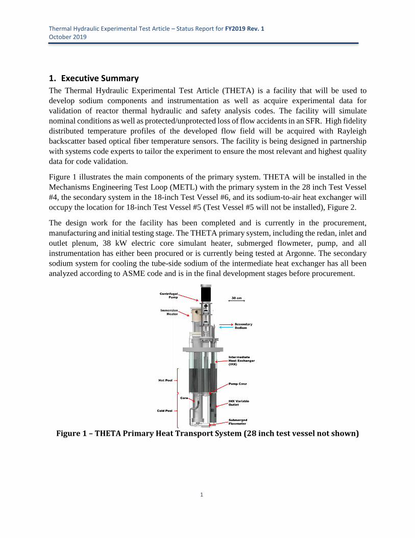
1. Executive Summary
The Thermal Hydraulic Experimental Test Article (THETA) is a facility that will be used to
develop sodium components and instrumentation as well as acquire experimental data for
validation of reactor thermal hydraulic and safety analysis codes. The facility will simulate
nominal conditions as well as protected/unprotected loss of flow accidents in an SFR. High fidelity
distributed temperature profiles of the developed flow field will be acquired with Rayleigh
backscatter based optical fiber temperature sensors. The facility is being designed in partnership
with systems code experts to tailor the experiment to ensure the most relevant and highest quality
data for code validation.
Figure 1 illustrates the main components of the primary system. THETA will be installed in the
Mechanisms Engineering Test Loop (METL) with the primary system in the 28 inch Test Vessel
#4, the secondary system in the 18-inch Test Vessel #6, and its sodium-to-air heat exchanger will
occupy the location for 18-inch Test Vessel #5 (Test Vessel #5 will not be installed), Figure 2.
The design work for the facility has been completed and is currently in the procurement,
manufacturing and initial testing stage. The THETA primary system, including the redan, inlet and
outlet plenum, 38 kW electric core simulant heater, submerged flowmeter, pump, and all
instrumentation has either been procured or is currently being tested at Argonne. The secondary
sodium system for cooling the tube-side sodium of the intermediate heat exchanger has all been
analyzed according to ASME code and is in the final development stages before procurement.
Figure 1 – THETA Primary Heat Transport System (28 inch test vessel not shown)

Thermal Hydraulic Experimental Test Article – Status Report for FY2019 Rev. 1 October 2019
2
Figure 2: Isometric drawing of THETA primary vessel (gray), secondary vessel (red), AHX (blue), and inter-vessel piping/valves (green), left. Location of THETA in METL
facility highlighted with red square, right.
2. Introduction
The Thermal Hydraulic Experimental Test Article (THETA) is a METL vessel experiment
designed for testing and validating sodium fast reactor components and phenomena. THETA has
been scaled using a non-dimensional Richardson number approach to represent temperature
distributions during nominal and loss of flow conditions in a sodium fast reactor (SFR). The
facility is being constructed with versatility in mind, allowing for the installation of various
immersion heaters, heat pipes, and heat exchangers without significant facility modification.
THETA is being designed in collaboration with systems code experts to inform the geometry and
sensor placement to acquire the highest value code validation data.
Scaling Approach
In order to scale an experimental facility, it is important to analyze the relevant non-dimensional
numbers. It has been shown in literature that the Richardson number predicts the temperature
distribution in a large stratified body of fluid such as the hot pool of a sodium fast reactor, Eq. 1
[1]–[4]:
𝑅𝑖 =𝐵𝑢𝑜𝑦𝑎𝑛𝑐𝑦
𝐼𝑛𝑒𝑟𝑡𝑖𝑎𝑙=
𝐺𝑟
𝑅𝑒2=
𝛽∆𝑇𝑔𝐷ℎ
𝑈2 (1)
Thermal Hydraulic Experimental Test Article – Status Report for FY2019 Rev. 1 October 2019
3
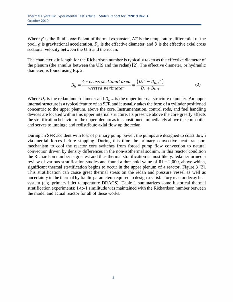
Where 𝛽 is the fluid’s coefficient of thermal expansion, ∆𝑇 is the temperature differential of the
pool, 𝑔 is gravitational acceleration, 𝐷ℎ is the effective diameter, and 𝑈 is the effective axial cross
sectional velocity between the UIS and the redan.
The characteristic length for the Richardson number is typically taken as the effective diameter of
the plenum (the annulus between the UIS and the redan) [2]. The effective diameter, or hydraulic
diameter, is found using Eq. 2.
𝐷ℎ =4 ∗ 𝑐𝑟𝑜𝑠𝑠 𝑠𝑒𝑐𝑡𝑖𝑜𝑛𝑎𝑙 𝑎𝑟𝑒𝑎
𝑤𝑒𝑡𝑡𝑒𝑑 𝑝𝑒𝑟𝑖𝑚𝑒𝑡𝑒𝑟=
(𝐷𝑟2 − 𝐷𝑈𝐼𝑆
2)
𝐷𝑟 + 𝐷𝑈𝐼𝑆 (2)
Where 𝐷𝑟 is the redan inner diameter and 𝐷𝑈𝐼𝑆 is the upper internal structure diameter. An upper
internal structure is a typical feature of an SFR and it usually takes the form of a cylinder positioned
concentric to the upper plenum, above the core. Instrumentation, control rods, and fuel handling
devices are located within this upper internal structure. Its presence above the core greatly affects
the stratification behavior of the upper plenum as it is positioned immediately above the core outlet
and serves to impinge and redistribute axial flow up the redan.
During an SFR accident with loss of primary pump power, the pumps are designed to coast down
via inertial forces before stopping. During this time the primary convective heat transport
mechanism to cool the reactor core switches from forced pump flow convection to natural
convection driven by density differences in the non-isothermal sodium. In this reactor condition
the Richardson number is greatest and thus thermal stratification is most likely. Ieda performed a
review of various stratification studies and found a threshold value of Ri = 2,000, above which,
significant thermal stratification begins to occur in the upper plenum of a reactor, Figure 3 [2].
This stratification can cause great thermal stress on the redan and pressure vessel as well as
uncertainty in the thermal hydraulic parameters required to design a satisfactory reactor decay heat
system (e.g. primary inlet temperature DRACS). Table 1 summarizes some historical thermal
stratification experiments; 1-to-1 similitude was maintained with the Richardson number between
the model and actual reactor for all of these works.

Thermal Hydraulic Experimental Test Article – Status Report for FY2019 Rev. 1 October 2019
4
Figure 3: Threshold of stratification occurrence in experimental studies of reactor
upper plenums. Plot adapted from [2]
Table 1: Summary of scaling parameters from some previous stratifications experiments from literature [2]. Note that the asterisk defines the non-dimensional
number as a ratio between the model and the actual reactor parameters. Experiment # Fluid Scale Ri* Pe* Re*
1 Na 1/6 1 0.07 0.09
2 Na 1/10 1 0.02 0.025
3 Na 1/10 1 - -
4 H2O 1/3 1 500 0.7
5 H2O 1/6 1 - -
6 H2O 1/7 1 - -
7 H2O 1/10 1 6 -
In order to scale an experiment to model the thermal hydraulic behaviors of a typical SFR, the
Richardson number should scale with one-to-one similitude, as seen in Table 1. During an
unprotected loss of flow accident (ULOF), core outlet temperature quickly rises without a
successful SCRAM of control rods and coolant flowrate drops as the pump spins down. Using
parameters from the Advanced Burner Test Reactor (ABTR) during a ULOF, Figure 4 [5], we
may propose nominal thermal hydraulic design parameters for THETA, Table 2.

Thermal Hydraulic Experimental Test Article – Status Report for FY2019 Rev. 1 October 2019
5
Figure 4: ABTR ULOF Transient Total Power and Channel 5 Flow, left. ABTR ULOF Transient Temperatures for Channel 5, right. [5]
Table 2: Comparison of parameters for Argonne National Laboratory’s Advanced
Burner Test Reactor (ABTR) and the proposed scaled reactor experiment Thermal
Hydraulic Experimental Test Article (THETA). Note that parameters for ABTR were
taken during 20% of nominal flow during a loss of flow incident. Volumetric thermal expansion (β) and density (ρ) taken from Fink and Leibowitz for sodium at 800 K [6]
Parameter: ABTR THETA
β 2.82E-4 [K-1] 2.82E-4 [K-1]
ρ 828.4 [kg/m3] 828.4 [kg/m3]
DUIS 1.3 [m] 0.20 [m]
Dr 4.9 [m] 0.64 [m]
Dh 3.61 [m] 0.43 [m]
Flowrate 7.57E-2 [m3/s] 3.15E-4 [m3/s]
(=1200 [GPM]) (=5 [GPM])
U 4.3E-3 [m/s] 1.1E-3 [m/s]
ΔT 90 [°C] 50 [°C]
Ri 48,450 [-] 48,562 [-]
Re 42,864 [-] 1,323 [-]
As one can see the Richardson number may be matched with one-to-one similitude with reasonable
experimental thermal hydraulic parameters. In Table 2 the Reynolds number for THETA is not
fully turbulent, a flow rate of approximately 19 GPM produces Re > 5,000 – a flow rate well within
the current primary pump curves, as will be introduced in a future section (Figure 38). Thus, the
effect of turbulence on the characteristics of thermal stratification may be studied.

Thermal Hydraulic Experimental Test Article – Status Report for FY2019 Rev. 1 October 2019
6
System Overview and Systems Code Application
THETA possesses all the major thermal hydraulic components of a pool type sodium cooled
reactor. A P&ID has been included in Figure 5 showing the primary and secondary sodium circuit.
A cross section of the primary vessel shows pool and core geometry, Figure 6. As can be seen, a
28” METL vessel is used for the primary sodium circuit and an 18” METL vessel is used for the
secondary sodium cooling system. An isometric model of the primary/secondary vessels, inter-
vessel piping, and air-to-sodium heat exchanger (AHX) can be found in Figure 2.
Figure 5: P&ID schematic of THETA

Thermal Hydraulic Experimental Test Article – Status Report for FY2019 Rev. 1 October 2019
7
Figure 6: THETA pool and core geometry. Core nominal diameter: 0.2 [m] (8”), core heated length: 0.3 [m] (12”) see heater geometry in Figure 41 for more information
THETA will be located on the METL mezzanine, in 28” and 18” nominal OD vessels, Figure 7
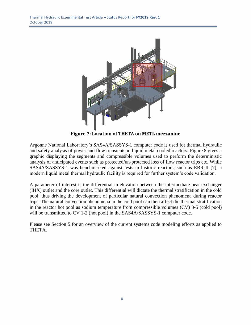
Thermal Hydraulic Experimental Test Article – Status Report for FY2019 Rev. 1 October 2019
8
Figure 7: Location of THETA on METL mezzanine
Argonne National Laboratory’s SAS4A/SASSYS-1 computer code is used for thermal hydraulic
and safety analysis of power and flow transients in liquid metal cooled reactors. Figure 8 gives a
graphic displaying the segments and compressible volumes used to perform the deterministic
analysis of anticipated events such as protected/un-protected loss of flow reactor trips etc. While
SAS4A/SASSYS-1 was benchmarked against tests in historic reactors, such as EBR-II [7], a
modern liquid metal thermal hydraulic facility is required for further system’s code validation.
A parameter of interest is the differential in elevation between the intermediate heat exchanger
(IHX) outlet and the core outlet. This differential will dictate the thermal stratification in the cold
pool, thus driving the development of particular natural convection phenomena during reactor
trips. The natural convection phenomena in the cold pool can then affect the thermal stratification
in the reactor hot pool as sodium temperature from compressible volumes (CV) 3-5 (cold pool)
will be transmitted to CV 1-2 (hot pool) in the SAS4A/SASSYS-1 computer code.
Please see Section 5 for an overview of the current systems code modeling efforts as applied to
THETA.

Thermal Hydraulic Experimental Test Article – Status Report for FY2019 Rev. 1 October 2019
9
Figure 8: Schematic of SAS4A/SASSYS-1 showing locations of various compressible volumes (CV#) and segments (S#)
3. Primary Vessel Component Summary The following section presents a summary of all primary vessel components as of August 2019,
Figure 9. Currently all components have been received, are being manufactured or final design
drawings are being sent in for manufacture.
Figure 9: THETA primary vessel components

Thermal Hydraulic Experimental Test Article – Status Report for FY2019 Rev. 1 October 2019
10
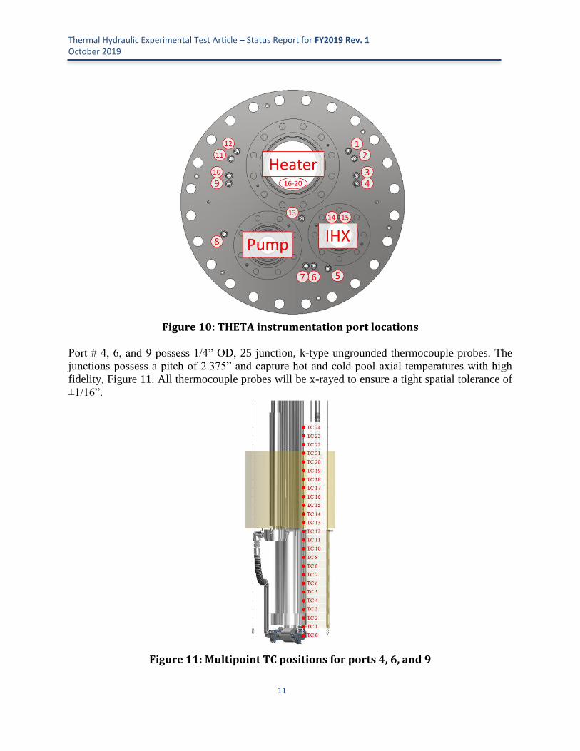
Instrumentation Table 3 summarizes THETA instrumentation which includes single and multi-point
thermocouples, distributed optical fiber temperature sensors, and flowmeter voltage
measurements. The port locations on the top flange have been labeled in Figure 10.
Table 3: THETA instrumentation and measurement. Port positions provided in Figure 10
Thermal Hydraulic Experimental Test Article – Status Report for FY2019 Rev. 1 October 2019
11
Figure 10: THETA instrumentation port locations
Port # 4, 6, and 9 possess 1/4” OD, 25 junction, k-type ungrounded thermocouple probes. The
junctions possess a pitch of 2.375” and capture hot and cold pool axial temperatures with high
fidelity, Figure 11. All thermocouple probes will be x-rayed to ensure a tight spatial tolerance of
±1/16”.
Figure 11: Multipoint TC positions for ports 4, 6, and 9

Thermal Hydraulic Experimental Test Article – Status Report for FY2019 Rev. 1 October 2019
12
Optical fiber temperature sensors will be used to acquire distributed temperature data at spatial
resolutions down to 0.65 mm and measurement rates of up to 250 Hz. These sensors are
constructed from single mode silica fibers, Figure 12. An ODISI 6104 optical fiber interrogator
system has been purchased and received from Luna Innovations, manufacturer specifications
provided in Table 4.
.
Figure 12: Photo showing 150 µm OD silica optical fiber
Table 4: ODISI 6104 spatial resolution and measurement rate
Spatial Resolution
[mm]
Measurement Rate
[Hz]
0.65 62.5
1.3 125
2.6 250
Optical fibers will be sheathed in a protective 1/16” OD 0.009” wall, 316 stainless steel capillary
tube to protect them from sodium. Given there are no connection points for the 1/16” capillaries
at the base of the 28” METL vessel, the optical fiber capillaries in ports 3, 7, and 10 will be
mechanically attached to 1/4” multipoint thermocouple probes in ports 4, 6, and 9 to provide
support, Figure 13 and Figure 14.

Thermal Hydraulic Experimental Test Article – Status Report for FY2019 Rev. 1 October 2019
13
Figure 13: Optical fiber capillaries mechanically coupled to 1/4” multi-junction
thermocouples
Figure 14: View of 3 optical fiber capillaries coupled to 1/4" multipoint
thermocouple probes
A custom sprung bellows assembly has been designed to provide tension and to make up any
thermal expansion differential between the 1/16” capillary tubes in ports 3, 7, 10, 13, and 14 and
the rest of the primary vessel components, Figure 15 and Figure 16. The total capillary length is
approximately 2 meters. Assuming an extremely conservative temperature differential between
capillary and inner vessel side walls of 250 °C, the maximum thermal expansion differential can
be calculated as 0.32” using a thermal expansion coefficient for stainless steel of 1.6 E-5 m/m-K.
Thus the bellows and spring should be able to account for expansion and contraction over a range
of 0.32” x 2 = 0.64”. A high temperature Inconel 600 spring with a free length of 1.75”, maximum

Thermal Hydraulic Experimental Test Article – Status Report for FY2019 Rev. 1 October 2019
14
deflection of 0.93” and linear spring rate of 12 lbs/in was sourced. To ensure the spring would not
permanently damage the capillary under tension a creep stress of 160 MPa was used (1% creep
rate in 10,000 hours at 550 C) to determine maximum spring force allowable on the 1/16” OD,
0.009” wall capillary. The maximum permissible deflection for the spring to prevent creep damage
to the capillary tube at high temperature was calculated as 2.93” using Eq 3. This is greater than
the maximum spring deflection of 0.93”, thus it would not be possible to yield the capillary tubes
with this assembly, even at elevated temperatures.
𝛿𝑚𝑎𝑥 =𝜎𝑐𝑟𝑒𝑒𝑝𝐴𝑐𝑎𝑝𝑖𝑙𝑙𝑎𝑟𝑦
𝛾 (3)
Where 𝜎𝑐𝑟𝑒𝑒𝑝 is the stress at 1% creep rate, 𝐴𝑐𝑎𝑝𝑖𝑙𝑙𝑎𝑟𝑦 is the cross sectional area of the capillary
tube, and 𝛾 is the linear spring coefficient.
Figure 15: Sprung bellows to makeup thermal expansion differential of 1/16"
capillaries, left. High temperature Inconel spring photo, right.
Figure 16: Picture of sprung bellows adapter

Thermal Hydraulic Experimental Test Article – Status Report for FY2019 Rev. 1 October 2019
15
Intermediate Heat Exchanger An intermediate heat exchanger has been designed to transfer heat from the THETA primary
sodium to its secondary sodium system. As can be seen in Figure 17, the current design is a shell
and tube type, with primary sodium on the shell side, and secondary sodium through a single U-
tube. Baffles with a 1/2 shell window cross section are used to promote thermal mixing in the
primary sodium, the top baffle possessing a deflector to prevent hot sodium impingement on the
cold secondary sodium downcomer tube, Figure 18. Thermal mixing of low Prandtl number fluids
can create a phenomenon known as thermal striping, where large magnitude temperature
oscillations occur. With high convection heat transfer inherent to liquid metals, a significant
amount of thermal stress can occur in piping [3]; the thermal striping deflector on the top baffle
prevents hot sodium entering the shell side from impinging directly on the cold secondary sodium
downcomer, thus reducing the thermal striping behavior. An expansion bellows on the secondary
sodium upcoming tube allows for the large thermal expansion differential between the two sides
of the U-tube. The design facilitates a 1/2” rod running concentric down the length of the shell to
allow for adjustment of the IHX primary sodium outlet elevation into the cold pool, as will be
discussed in a later section.
Figure 17: Shell and tube intermediate heat exchanger

Thermal Hydraulic Experimental Test Article – Status Report for FY2019 Rev. 1 October 2019
16
Figure 18: Intermediate heat exchanger shell side baffle, left. Top baffle showing
thermal striping deflector feature, right.
The heat exchanger was sized using the effectiveness-NTU method for one shell pass and two
tube passes (single U-tube). This method identifies the maximum possible heat transfer rate and
uses a calculated effectiveness to determine the actual heat transfer rate, Eq. 4.
�̇� = 휀�̇�𝑚𝑎𝑥 (4)
The effectiveness for a heat exchanger of this type as a function of transfer units and capacity ratio
can be found in Eq. 5.
휀 = 2
[
1 + 𝐶𝑅 + √1 + 𝐶𝑅2
1 + exp (−𝑁𝑇𝑈√1 + 𝐶𝑅2)
1 − exp (−𝑁𝑇𝑈√1 + 𝐶𝑅2)
] −1
(5)
Where 𝐶𝑅 is a dimensionless number referred to as the capacity ratio, comparing the capacitance
rates of the tube and the shell side fluids, Eq. 6, and NTU is the number of transfer units, calculated
using Eq. 7.
𝐶𝑅 =
�̇�𝑚𝑖𝑛
�̇�𝑚𝑎𝑥
(6)
Where �̇�𝑚𝑖𝑛 and �̇�𝑚𝑎𝑥 are the minimum and maximum of the capacitance rates of fluid on either
side of the heat exchanger.
𝑁𝑇𝑈 =
𝑈𝐴
�̇�𝑚𝑖𝑛
(7)
The conductance of the heat exchanger, 𝑈𝐴, is a function of both geometry and heat transfer in the
heat exchanger. The conductance may be found by taking the inverse of the total thermal
resistance, Eq. 8.
𝑈𝐴 =
1
𝑅𝑡𝑜𝑡
=1
𝑅ℎ,𝑡𝑢𝑏𝑒 + 𝑅𝑘 + 𝑅ℎ,𝑠ℎ𝑒𝑙𝑙 + 𝑅𝑓
(8)
Where 𝑅ℎ,𝑡𝑢𝑏𝑒 is the convection resistance from the tube fluid to the tube inner wall, 𝑅𝑘 is the
resistance to conduction in the tube wall, 𝑅ℎ,𝑠ℎ𝑒𝑙𝑙 is the convection resistance from the shell fluid
to the tube outer wall, and 𝑅𝑓 is the resistance due to fouling. According to literature the fouling
resistance in alkali metal heat exchangers is negligible if oxide level is kept below a few wppm

Thermal Hydraulic Experimental Test Article – Status Report for FY2019 Rev. 1 October 2019
17
[8]. The convection resistance may be determined with the use of the Nusselt number. On the tube
side, the Nusselt number was found using a correlation for NaK flowing through a tube [9], Eq. 9.
𝑁𝑢 = 4.82 + 0.0185 ∙ 𝑃𝑒0.827 (9)
On the shell side, the Nusselt number was found using a correlation for in-line flow through un-
baffled rod bundles in wide spaced arrays (tube pitch / tube diameter = P/D > 1.35) [10], Eq. 10.
Note that P/D for the above THETA IHX is 1.6.
𝑁𝑢 = 6.66 + 3.126
𝑃
𝐷+ 1.84 (
𝑃
𝐷)
2
+ 0.0155(�̅�𝑃𝑒)0.86
(10)
Where �̅�, the ratio between eddy diffusivities of heat and momentum, is generally assumed equal
to one [11].
Kern’s method was used to estimate shell side pressure drop across the heat exchanger, Eq. 11
[12].
∆𝑃𝐾𝑒𝑟𝑛𝑠 = 8𝑗𝑓 (𝐷𝑠
𝑑𝑒) (
𝐿
𝑙𝐵)𝜌𝑢𝑠
𝑠
2(
𝜇
𝜇𝑤)−0.14
(11)
Where 𝑗𝑓 is a friction factor found using Figure 19 [12], 𝐷𝑠 is the shell side inner diameter, 𝑑𝑒 is
the hydraulic diameter, 𝐿 is the tube length, 𝑙𝐵 is the baffle spacing, 𝜌 is the process fluid density,
𝑢𝑠 is the shell side linear velocity, and 𝜇
𝜇𝑤 is a ratio of viscosity in the bulk fluid as compared to
viscosity at the wall—in general this term may be neglected for low viscosity fluids such as
sodium.
Figure 19: Shell side friction factors, segmental baffles, adapted from [12]

Thermal Hydraulic Experimental Test Article – Status Report for FY2019 Rev. 1 October 2019
18
Alternatively, and as a second check, the pressure drop across the shell side of the IHX may be
approximated with the use of minor loss coefficients by treating each baffle as an expansion and
contraction as the fluid flows from one baffle window to the next, Eq. 12.
∆𝑃𝑚𝑖𝑛𝑜𝑟−𝑙𝑜𝑠𝑠 = 𝑁𝑏(𝐾𝑐𝑜𝑛𝑡𝑟𝑎𝑐𝑡𝑖𝑜𝑛 + 𝐾𝑒𝑥𝑝𝑎𝑛𝑠𝑖𝑜𝑛)𝜌𝑢𝑠
𝑠
2 (12)
Where 𝑁𝑏 is the number of baffles and 𝐾𝑐𝑜𝑛𝑡𝑟𝑎𝑐𝑡𝑖𝑜𝑛 and 𝐾𝑒𝑥𝑝𝑎𝑛𝑠𝑖𝑜𝑛 are the minor loss coefficients
found in [13].
Using the thermal hydraulic parameters given in Table 5, the performance of the THETA IHX
may be predicted. As can be seen the secondary sodium system flowrate was set to 5 GPM, the
primary sodium inlet temperature was set to 350 °C, the secondary sodium inlet temperature was
set to 250 °C. The shell side temperature differential and head as a function of shell side flow rate
can be found plotted in Figure 20. As can be seen, the Kern’s method and minor loss method agree
very well, there is a lack of smoothness in the Kern’s method curve due to slight inaccuracies in
graphically calculating friction factors from Figure 19.
Table 5: Intermediate heat exchanger sizing parameters
Parameter Value Unit Q
sodium,secondary 5 GPM
Tsodium,primary,in
350 °C T
sodium,secondary,in 250 °C

Thermal Hydraulic Experimental Test Article – Status Report for FY2019 Rev. 1 October 2019
19
Figure 20: IHX predicted shell side temperature differential and head as a function of shell side flow rate
The IHX possesses a variable height outlet mechanism allowing for deposition of cold sodium at
various elevations in the cold pool to study the transient and steady state temperature profile which
develop throughout an SFR as a result of changing this variable, Figure 21. Depositing cold sodium
at a lower elevation in the cold pool is predicted to result in more stratification and ultimately result
in a more thermally stratified hot pool. This will be an important variable to study for the
development of reactor codes. Figure 22 shows drawings of the inner and outer barrel. As can be
seen there are qty. (6) 2.75” square windows at elevations spaced 4.5” apart from center to center.
The inner barrel rests on a stainless steel cone on the bottom of the outer barrel in a Hastelloy C-
276 seat, reducing the likelihood of galling.
0 5 10 15 2020
40
60
80
100
0
0.125
0.25
0.375
Vshell,GPM
Shell S
ide D
T
[°C
]
Head [
in]
Minor Loss MethodMinor Loss Method
Kern's MethodKern's Method
Temperature Differential and Head vs Shell Flow Rate

Thermal Hydraulic Experimental Test Article – Status Report for FY2019 Rev. 1 October 2019
20
Figure 21: IHX Outlet dimension, top. Isometric model of variable elevation IHX outlet, bottom left. Drawing showing predicted cold pool temperature distribution as
a function of IHX outlet window elevation, (red = hot, purple = warm, blue = cold), bottom right.

Thermal Hydraulic Experimental Test Article – Status Report for FY2019 Rev. 1 October 2019
21
Figure 22: Variable elevation IHX outlet. Drawings showing the inner barrel, left, outer barrel, middle, and the assembly of inner/outer barrel and actuator stem,
right.
CFD Analysis of Hot Pool
A computational fluid dynamic simulation was performed with Ansys CFX 19.2 to assess the
performance of the intermediate heat exchanger and acquire a preliminary predicted temperature
distribution of the hot pool during steady state operation of THETA. The domains, boundary
conditions and meshing from this analysis are shown in Figure 23. As can be seen an adiabatic
‘flow-blocker’ simulating the heater element spacer plate, and ultimately the UIS of an SFR, was
added to distribute flow more realistically in the hot pool. The mesh was constructed of 815,325
tetrahedral elements utilizing inflation layers in and around the IHX to accurately capture the low
Prandtl number heat transfer in this region. All sodium thermal hydraulic material properties were
set to a constant value for sodium at 300 °C, these values taken from [6].

Thermal Hydraulic Experimental Test Article – Status Report for FY2019 Rev. 1 October 2019
22
Figure 23: THETA CFD domains and boundary conditions (left), mesh wireframe showing high mesh density near IHX (right)
The CFD simulation flowrate and temperature inputs for the primary and secondary sodium
domains have been provided in Table 6. These parameters were also used for analytical
calculations using heat exchanger correlations as previously detailed in Section 3.2 of this report.
Table 6: CFD and analytical calculation input parameters CFD and Analytical Inputs:
Primary Flow Rate 5 GPM
Secondary Flow Rate 5 GPM
Primary Inlet Temp 270 °C
Secondary Inlet Temp 200 °C
Temperature and velocity profiles of interest have been highlighted in Figure 24. As can be seen,
a stratified temperature profile develops in the bulk sodium of the hot pool. Downward velocity
streamlines are visible in close proximity to the IHX, showing a developed large scale natural
convection driven flow.

Thermal Hydraulic Experimental Test Article – Status Report for FY2019 Rev. 1 October 2019
23
Figure 24: Temperature profile of hot pool and IHX with velocity streamlines
(top,left), 3D temperature profile (top,right), velocity profile of hot pool and IHX (bottom, left), velocity streamlines of hot pool and IHX (bottom, right)
A summary of the average primary sodium outlet temperature from the IHX found with CFD and
by analytical heat exchanger correlations, method detailed in the Section 3.2, can be found in Table
7. As can be seen the two analysis methods show great correlation, with the average outlet
temperature within 2 °C.
Table 7: CFD and analytical results showing good correlation between two calculation methods ANSYS CFX CFD Results:
Primary Average Outlet Temp 244 °C
Primary Power Dissipation 9.5 kW
Analytical Results Using HX Correlations:
Primary Average Outlet Temp. 242 °C
Primary Power Dissipation 10.46 kW

Thermal Hydraulic Experimental Test Article – Status Report for FY2019 Rev. 1 October 2019
24
Submersible Flowmeter A submersible permanent magnet flowmeter has been designed to acquire primary sodium
flowrate, Figure 25. The flowmeter uses a magnetic field generated by high temperature
Samarium-Cobalt (SmCo) magnets, oriented perpendicular to sodium flow, to generate a Lorentz
current that is linearly proportional to flow. The measured voltage signal, 𝑉𝑚, is read with two
pickup wires oriented diametrically across the flow tube and is related to sodium flowrate via Eq.
13 [14], [15].
Figure 25: Submersible permanent magnet flowmeter
𝑉𝑚 = 𝐾1𝐾2𝐾3
4𝐵𝑄
𝜋𝑑2 (13)
Where the K factors account for geometric and material properties, B is the magnetic field strength
measured at the central plane of the magnets, at the center of the sodium flow, Q is the sodium
volumetric flowrate, and d is the inner diameter of the sodium flow-tube. The K factors are given
in Eqs. 13-15.
𝐾1, Eq. 14, accounts for the “shunting” effect, whereby the sodium containment can reduce the
measured signal depending on material electrical resistivity and the geometry.
𝐾1 =
2𝑑/𝐷
[1 + (𝑑𝐷)
2
] + (𝜌𝑓
𝜌𝑤) [1 − (
𝑑𝐷)
2
]
(14)
Where D is the outer diameter of the sodium flow-tube, 𝜌𝑓 is the resistivity of the liquid metal,
and 𝜌𝑤 is the resistivity of the containment material. As the permanent magnets are not infinitely
long, end effects are accounted for with 𝐾2, Eq. 15.
𝐾2 = −0.0047 (𝐿
𝑑)4
+ 0.0647 (𝐿
𝑑)3
− 0.3342 (𝐿
𝑑)
2
+ 0.77 (15)

Thermal Hydraulic Experimental Test Article – Status Report for FY2019 Rev. 1 October 2019
25
Where L is the length of the permanent magnets in the direction of sodium flow. 𝐾3, Eq. 16,
accounts for temperature effect on the permanent magnet.
𝐾3 =(−7𝐸 − 07)𝑇3 − 0.0002𝑇 + 0.8587
0.8587 (16)
Where T is the temperature of the permanent magnet in degrees Celsius. Eq. 16 was found by
fitting a quadratic function to the residual induction as a function of temperature, as provided by
the manufacturer, Figure 26. The particular magnetic material used in this flowmeter is from
Electron Energy Corporation, product number EEC SmCo 2:17-18 T550. This grade of SmCo has
shown resistance to magnetic field degradation with a neutron flux of 1018 n/cm2 and temperatures
≤ 550 °C [16].
Figure 26: Manufacturer (Electron Energy Corporation) provided BH curve as a
function of temperature, left. Residual induction as a function of temperature for SmCo T550 high temperature magnets from Electron Energy Corporation, right.
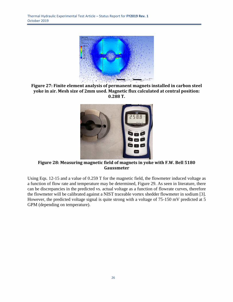
In order to acquire the magnetic field at the flowmeter center, an Ansys Maxwell finite element
simulation was performed to calculate 3D magnetic flux field, Figure 27. The flux density at the
center of the flow tube along the center plane of the magnets was calculated as 0.288 T. Using an
F.W. Bell 5180 Gaussmeter, the magnetic flux at the center position of the as built magnet
assembly was measured as 0.259 T, Figure 28.
Thermal Hydraulic Experimental Test Article – Status Report for FY2019 Rev. 1 October 2019
26
Figure 27: Finite element analysis of permanent magnets installed in carbon steel
yoke in air. Mesh size of 2mm used. Magnetic flux calculated at central position: 0.288 T.
Figure 28: Measuring magnetic field of magnets in yoke with F.W. Bell 5180
Gaussmeter
Using Eqs. 12-15 and a value of 0.259 T for the magnetic field, the flowmeter induced voltage as
a function of flow rate and temperature may be determined, Figure 29. As seen in literature, there
can be discrepancies in the predicted vs. actual voltage as a function of flowrate curves, therefore
the flowmeter will be calibrated against a NIST traceable vortex shedder flowmeter in sodium [3].
However, the predicted voltage signal is quite strong with a voltage of 75-150 mV predicted at 5
GPM (depending on temperature).

Thermal Hydraulic Experimental Test Article – Status Report for FY2019 Rev. 1 October 2019
27
Figure 29: Voltage signal as a function of sodium flow rate and temperature
Samarium cobalt magnets possess a strong pull force, thus precautions must be taken when
assembling the flowmeter yoke to prevent injury and/or damage to the brittle magnets. As can be
seen in Figure 30, a wooden jig for assembling the magnet assembly was constructed; wooden
tracks were used to direct the magnet into position on the yoke, using plastic shims to slowly allow
the magnet to approach the yoke. The yoke/magnet assembly may then be slid into the outer tube
for final seal welding with top cap, Figure 31.
Figure 30: Magnet/yoke assembly using wooden tracks and plastic shims, left.
Assembled magnet/yoke assembly, right.

Thermal Hydraulic Experimental Test Article – Status Report for FY2019 Rev. 1 October 2019
28
Figure 31: Magnet/yoke installation, left. Top cap prepared for final welding, right.
Careful attention was paid to the method of attaching the sensor wires to the flow tube as the
electrical resistance created by a poorly attached wire can affect signal readings. A series of
mockups were created with various attachment techniques, Figure 32. The final attachment scheme
was to weld a 0.187” diameter ‘wire nub connector’ with a weep hole, then braze the 1/16” 316SS
sensor wire to this nub connector using a high temperature (760 °C liquidous) Ag-Cu alloy, Figure
33.
Figure 32: Mockups of sensor wire attachment methods

Thermal Hydraulic Experimental Test Article – Status Report for FY2019 Rev. 1 October 2019
29
Figure 33: Connection of sensor wire to flow tube in submersible permanent magnet
flowmeter. Attachment of wire nub connector via welding and brazing, left, detail drawing of wire nub connector, right.
The method for attaching the mineral insulated cable to the flowmeter feedthrough under sodium
can be found in Figure 34. As can be seen a protective housing is swaged over a high temperature
brazed connection between the 316SS sensor wires and the constantan wires on the MI cable.
Precautions were taken when welding the flowmeter together to avoid exposing the magnets to
high temperature. Most of the flowmeter welds were made without magnets installed and during
final welds, with magnets installed, copper heat sinks and a continuous argon purge over the
magnets were used to dissipate welding heat, Figure 35. The magnetic field was measured post-
welding and there was no detectible degradation in magnetic field strength found, Figure 35
Figure 34: Sensor wire feedthrough from flowmeter to mineral insulated wire.

Thermal Hydraulic Experimental Test Article – Status Report for FY2019 Rev. 1 October 2019
30
Figure 35: Copper heat sinks and argon purge during welding (left), magnetic field measurement post welding end cap onto outer shell
Pump The primary sodium centrifugal pump has been received from Wenesco Inc., Figure 36, and
installed in a water testing rig as seen in Figure 37. The P&ID of the flow circuit for water testing
the pump can be found in Figure 37 as well which was used to develop detailed flow curves for
the pump, Figure 38.
Figure 36: Pump as delivered, left, 4.5" OD impeller, right.

Thermal Hydraulic Experimental Test Article – Status Report for FY2019 Rev. 1 October 2019
31
Figure 37: Wenesco centrifugal pump mounted for water testing (left). P&ID for water testing (right)
Figure 38: Pump curves made using water at 27 °C as surrogate fluid. System curves
shown for primary and secondary sodium.
An all stainless steel flexible metal hose has been acquired that will be located at the pump case
outlet to account for piping thermal expansion and any mechanical/hydraulic vibration, Figure 39.
The electrical enclosures for THETA pump and heater control as well as data acquisition have
Pump
Gate ValveFlowmeter
Drum
Differential Pressure w/ 3-way Manifold

Thermal Hydraulic Experimental Test Article – Status Report for FY2019 Rev. 1 October 2019
32
been completed and are currently being tested for proper functionality by performing the primary
pump water testing / pump curve formulation, Figure 40.
Figure 39: Swagelok FX stainless steel flexible hose for case outlet, left, model showing placement at outlet of pump case, right
Figure 40: 240 VAC, 480 VAC and 24 VDC electrical enclosures
Immersion Heater The immersion heater and associated electrical enclosure have been received from Chromalox,
Figure 41. Heater elements were tested with multimeter to ensure proper rated resistance of ~35
ohms, ensuring no significant damage resulted during shipment. The immersion heater is currently
in storage in a climate controlled room with desiccant bags to prevent moisture ingress into the
heater elements.

Thermal Hydraulic Experimental Test Article – Status Report for FY2019 Rev. 1 October 2019
33
Figure 41: Chromalox 38 kW Immersion Heater (top). Heater control system electrical enclosure (bottom).
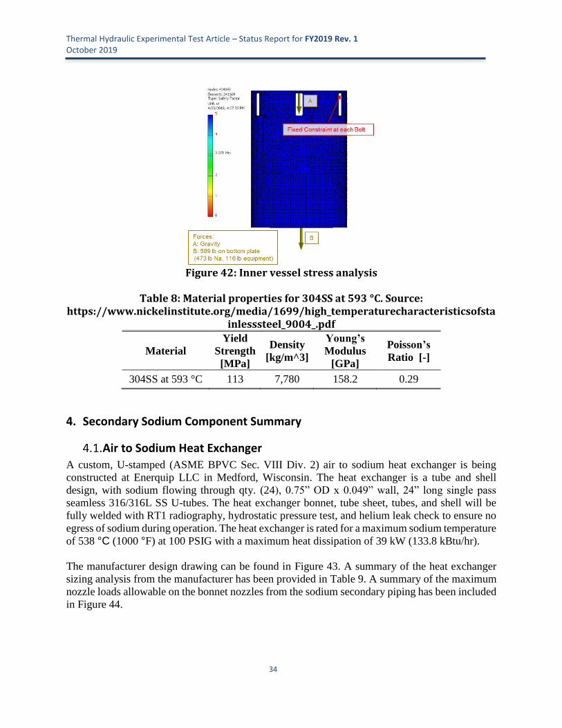
Inner Vessel Stress Analysis A finite element analysis was performed using Autodesk Inventor’s stress analysis software on
inner vessel to ensure >2x factor of safety with hot pool full of sodium without any upward
buoyancy force from the cold pool supporting load. The mesh, loads/constraints and safety factor
(as a function of yield strength) are all detailed in Figure 42. A summary of the material property
used for this analysis can be found in Table 8. The analysis showed a factor of safety of 3.1 for
yield strength of 304SS at 593 °C.
8”
Thermal Hydraulic Experimental Test Article – Status Report for FY2019 Rev. 1 October 2019
34
Figure 42: Inner vessel stress analysis
Table 8: Material properties for 304SS at 593 °C. Source:
https://www.nickelinstitute.org/media/1699/high_temperaturecharacteristicsofstainlesssteel_9004_.pdf
Material
Yield
Strength
[MPa]
Density
[kg/m^3]
Young’s
Modulus
[GPa]
Poisson’s
Ratio [-]
304SS at 593 °C 113 7,780 158.2 0.29
4. Secondary Sodium Component Summary
Air to Sodium Heat Exchanger
A custom, U-stamped (ASME BPVC Sec. VIII Div. 2) air to sodium heat exchanger is being
constructed at Enerquip LLC in Medford, Wisconsin. The heat exchanger is a tube and shell
design, with sodium flowing through qty. (24), 0.75” OD x 0.049” wall, 24” long single pass
seamless 316/316L SS U-tubes. The heat exchanger bonnet, tube sheet, tubes, and shell will be
fully welded with RT1 radiography, hydrostatic pressure test, and helium leak check to ensure no
egress of sodium during operation. The heat exchanger is rated for a maximum sodium temperature
of 538 °C (1000 °F) at 100 PSIG with a maximum heat dissipation of 39 kW (133.8 kBtu/hr).
The manufacturer design drawing can be found in Figure 43. A summary of the heat exchanger
sizing analysis from the manufacturer has been provided in Table 9. A summary of the maximum
nozzle loads allowable on the bonnet nozzles from the sodium secondary piping has been included
in Figure 44.

Thermal Hydraulic Experimental Test Article – Status Report for FY2019 Rev. 1 October 2019
35
Figure 43: Manufacturer design drawing of tube-and-shell type air-to-sodium heat
exchanger

Thermal Hydraulic Experimental Test Article – Status Report for FY2019 Rev. 1 October 2019
36
Figure 44: Maximum permissible nozzle loading on AHX bonnet nozzles are given in
the column for “Load case 2.” This information was used to set a limit for stress imposed by secondary piping during B31.3 pipe analysis.

Thermal Hydraulic Experimental Test Article – Status Report for FY2019 Rev. 1 October 2019
37
Table 9: Air-to-sodium heat exchanger specification sheet

Thermal Hydraulic Experimental Test Article – Status Report for FY2019 Rev. 1 October 2019
38
Secondary Sodium Piping The secondary sodium system transfers sodium from the tube side of the intermediate heat
exchanger, then to the auxiliary 18” vessel, then to the air-to-sodium heat exchanger, then back to
the intermediate heat exchanger. A thermal stress analysis has been performed on the secondary
sodium system by JEH Consulting with CAESAR II computer software to acquire a Professional
Engineer stamp ensuring compliance with ASME B31.3 pipe code. The piping analysis
demonstrated passing of pipe code under all extreme and nominal operating conditions.
The secondary piping system is seamless 3/4” SCH 40 piping made with 316H stainless steel
(ASTM 376 type 316H) given its superior strength at high temperature as compared to other grades
of 300 series stainless. All of the fittings are 3/4” SCH 40 316/316L seamless tubes. Originally the
fittings were specified as 316H, however during procurement it was found that these were not
readily available from a domestic or DFARs compliant supplier. 316/316L (ASTM A182 Type
F316 or ASTM A403 Type WP316) possesses the same strength rating as 316H up to and including
1000 °F and is more readily available, therefore the fittings were specified using this grade of
stainless.
The maximum temperature limit of the system is 1000 °F and the system has a design pressure of
50 PSIG. A total of six scenarios were identified for analysis to bound all possible operating
conditions, Table 10, Table 11. A screenshot of the CAESAR-II software setup to test Scenarios
1-6 can be found in Figure 46. Note the maximum temperature of 1000 °F and the corresponding
minimum temperature of 790 °F during nominal operating conditions with the AHX operating at
full duty. A screen shot of the exaggerated overall thermal expansion of the system can be found
in Figure 47, and quantitative maximum expansion in the x, y, z coordinates can be found in Figure
48.
Table 10: 6 operating scenarios for secondary sodium system to test for thermal stress analysis. Locations referenced can be found in Figure 45

Thermal Hydraulic Experimental Test Article – Status Report for FY2019 Rev. 1 October 2019
39
Table 11: Summary of operating load cases
Figure 45: Piping locations for thermal stress analysis

Thermal Hydraulic Experimental Test Article – Status Report for FY2019 Rev. 1 October 2019
40
1
2
3
4
5
6
Figure 46: Screenshot of CAESAR-II software with setup for testing Scenarios 1-6. Orange = 1000 °F, purple = 790 °F, except for scenario 4 where purple = 0 °F.

Thermal Hydraulic Experimental Test Article – Status Report for FY2019 Rev. 1 October 2019
41
Figure 47: Visualization of thermal expansion, displacement exaggerated to allow for
understanding of overall movement.

Thermal Hydraulic Experimental Test Article – Status Report for FY2019 Rev. 1 October 2019
42
(a)
(b)
(c)
Figure 48: Maximum displacements: (a) 0.64” maximum in the +x direction (b) 0.57” in the -y direction (c) 0.90” in the –z direction .

Thermal Hydraulic Experimental Test Article – Status Report for FY2019 Rev. 1 October 2019
43
5. THETA Model Development
Modeling of the Thermal Hydraulic Experimental Test Article (THETA) experiment has been
performed using the SAS4A/SASSYS-1 fast reactor safety analysis code. A THETA model has
been developed to represent the THETA experiment design developed at Argonne to demonstrate
the importance of key elevations on natural circulation flow rates. The model currently includes
the core channel and the primary heat transport system of the THETA experimental facility.
Core Channel
In SAS4A/SASSYS-1, the thermal-hydraulic performance of a reactor core is analyzed with a
model consisting of single-pin channels. A single-pin channel represents the average pin in an
assembly, and assemblies with similar reactor physics and thermal-hydraulic characteristics are
grouped together. A number of channels can be selected to represent all assemblies in the reactor
core.
In the THETA experiment, a heater consisting of 27 U-shape heating elements was used as a fuel
assembly. Therefore, the THETA model assumed one channel that has 54 “nuclear fuel” pins. The
properties of the fuel were simulated using MgO properties and Incoloy 800 properties for
cladding. SAS requires a fission gas plenum in the fuel region so the unheated region in the heater
was assumed to be the fission gas plenum, and the properties of the fission gas were assumed to
be the properties of MgO to minimize the impact of fission gas plenum. We assumed a 1 cm
reflector above and below the fuel region. Three zones comprise the core channel as shown in
Figure 49. Zone 1 is the lower reflector. Zone 2 includes both the fuel and fission gas plenum.
Zone 3 represents the upper reflector.

Thermal Hydraulic Experimental Test Article – Status Report for FY2019 Rev. 1 October 2019
44
Figure 49. Geometry of core channel of THETA model
Primary Heat Transport System
The PRIMAR-4 module in SAS4A/SASSYS-1 simulates the thermal hydraulics of the heat
transport systems. In a PRIMAR-4 model, compressible volumes, or CVs, are zero-dimensional
volumes that are used to model larger volumes of coolant such as inlet and outlet plena and pools.
CVs are characterized by their pressure, temperature, elevation, and volume. Compressible
volumes are connected by liquid segments, which are composed of one or more elements.
Elements are modeled by one-dimensional, incompressible, single-phase flow and can be used to
model pipes, valves, heat exchangers, steam generators, and more. Elements are characterized by
their pressure, temperature, elevation, and mass flow rate.
Figure 50 illustrates the PRIMAR-4 model of the primary heat transport system of THETA
experiment. Sodium enters Segment 1, which represents the core channel, from the inlet plenum,
Compressible Volume 1 (CV1). Sodium discharges from the core into the hot pool, CV2, before
flowing into the intermediate heat exchanger (IHX) in Segment 2 and out into the cold pool, CV3.
The IHX was modeled using a table look-up IHX model. The IHX outlet flow distributor is
modeled using Element 4 with varying elevation of outlet and length and Element 5 with varying
inlet and outlet elevations. The primary system flow circuit is completed as sodium flows in
Segment 3, representing the sodium pump and its corresponding heater inlet piping, before
discharging into the inlet plenum. The sodium pump was modeled using a pump-head-versus-time
table look-up pump model. All compressible volumes are currently modeled using the standard
zero-dimensional volume treatment in SAS4A/SASSYS-1.

Thermal Hydraulic Experimental Test Article – Status Report for FY2019 Rev. 1 October 2019
45
Figure 50. PRIMAR-4 model of the primary heat transport system of THETA experiment
Transients Analysis
ULOF Analysis
Unprotected loss of flow (ULOF) transient simulations were performed using the THETA model
described above. This transient assumes a pump trip without coastdown at 10 seconds. Heater
power was assumed to remain constant at 18 kW. It was assumed that the IHX provides the same
temperature change (50 °C) over the transient process.
Figure 51.1 illustrates the segment flows. The segment flow rates decreased sharply after the pump
trip because it was assumed that there is no coastdown. Then, flow rates increased due to the
temperature difference between hot pool (CV2) and cold pool (CV3) as shown in Figure 51.2. The

Thermal Hydraulic Experimental Test Article – Status Report for FY2019 Rev. 1 October 2019
46
hot pool and cold pool surface levels corresponded to the temperature behavior as shown in Figure
51.3. Figure 51.4 and Figure 51.5 show the difference in the pump segment flow rates and window
outlet temperatures between window option1 (upper most window) and window option 6 (lower
most window). Window 1 has slightly higher flow rates after 400 seconds compared to window 6.
This is due to the higher thermal driving force of the natural circulation for window 1. The out of
window temperature delays in window 6 compare to window 1 because it takes more time for
sodium coolant to reach window 6 than window 1.
Figure 51.6 illustrates the peak fuel, cladding, and coolant temperatures. After the pump trip at 10
seconds, the fuel, cladding, and coolant temperatures begin to increase, reaching a maximum in
about 245 seconds. Afterwards, the temperatures begin to decrease and enter the equilibrium state
as the flow rate increases due to the natural circulation. Window1 and Window6 showed the
differences in temperatures after 400 seconds.
0
0.05
0.1
0.15
0.2
0.25
0.3
0.35
0 200 400 600 800 1000
Segment Flows
Core_Window1IHX_Window1Pump_Window1Core_Window6IHX_Window6Pump_Window6
Flo
w R
ate
(kg/s
)
Time (s)
180
200
220
240
260
280
300
320
0 200 400 600 800 1000
Pool Temperatures
CV1_Window1CV2_Window1CV3_Window1Window1 OutletCV1_Window6CV2_Window6CV3_Window6Window6 Outlet
Tem
pera
ture
(°C
)
Time (s)

Thermal Hydraulic Experimental Test Article – Status Report for FY2019 Rev. 1 October 2019
47
Figure 51.1-6 (left to right by consecutive row) LOF Transient Results.
USBO Analysis
Unprotected station blackout (USBO) transient simulations were also performed using the THETA
model described above. This transient assumed a pump trip without coastdown at 10 seconds.
Heater power was assumed to remain constant at 18 kW. It was assumed that IHX stops removing
heat at 10 seconds. In addition to that, the orifice coefficient of IHX was changed from 10 to 200
to get a reasonable pressure drop in the IHX.
Figure 52.1 illustrates the segment flow rates. Again, the segment flow rates decreased sharply
after the pump trip because it was assumed that there is no coastdown. Then flow rates increased
due to the temperature difference between CV2 and CV3 as shown in Figure 52.2. The hot pool
and cold pool surface levels corresponded to the temperature behavior as shown in Figure 52.3.
1.16
1.165
1.17
1.175
1.18
0 200 400 600 800 1000
Pool Surface Levels
Hot Pool_Window1Cold Pool_Window1Hot Pool_Window6Cold Pool_Window6
Ele
va
tio
n (
m)
Time (s)
0
0.05
0.1
0.15
0.2
0.25
0.3
0.35
0 200 400 600 800 1000
Pump Segment Flows
Pump Flow Rate_Window 1
Pump Flow Rate_Window 6
Flo
w R
ate
(kg/s
)
Time (s)
180
190
200
210
220
230
240
0 200 400 600 800 1000
Out of Window Temperatures
Window1 OutletWindow6 Outlet
Tem
pera
ture
(°C
)
Time (s)
200
250
300
350
400
450
500
0 200 400 600 800 1000
Peak Core Temperatures
Coolant_Window1Cladding_Window1Fuel_Window1Coolant_Window6Cladding_Window6Fuel_Window6
Tem
pera
ture
(°C
)
Time (s)
Thermal Hydraulic Experimental Test Article – Status Report for FY2019 Rev. 1 October 2019
48
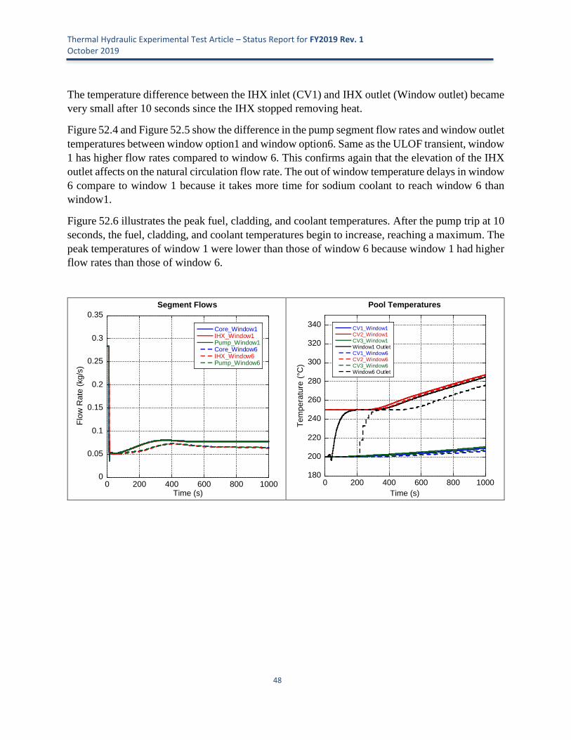
The temperature difference between the IHX inlet (CV1) and IHX outlet (Window outlet) became
very small after 10 seconds since the IHX stopped removing heat.
Figure 52.4 and Figure 52.5 show the difference in the pump segment flow rates and window outlet
temperatures between window option1 and window option6. Same as the ULOF transient, window
1 has higher flow rates compared to window 6. This confirms again that the elevation of the IHX
outlet affects on the natural circulation flow rate. The out of window temperature delays in window
6 compare to window 1 because it takes more time for sodium coolant to reach window 6 than
window1.
Figure 52.6 illustrates the peak fuel, cladding, and coolant temperatures. After the pump trip at 10
seconds, the fuel, cladding, and coolant temperatures begin to increase, reaching a maximum. The
peak temperatures of window 1 were lower than those of window 6 because window 1 had higher
flow rates than those of window 6.
0
0.05
0.1
0.15
0.2
0.25
0.3
0.35
0 200 400 600 800 1000
Segment Flows
Core_Window1IHX_Window1Pump_Window1Core_Window6IHX_Window6Pump_Window6
Flo
w R
ate
(kg/s
)
Time (s)
180
200
220
240
260
280
300
320
340
0 200 400 600 800 1000
Pool Temperatures
CV1_Window1CV2_Window1CV3_Window1Window1 OutletCV1_Window6CV2_Window6CV3_Window6Window6 Outlet
Tem
pera
ture
(°C
)
Time (s)

Thermal Hydraulic Experimental Test Article – Status Report for FY2019 Rev. 1 October 2019
49
Figure 52.1-6 (left to right by consecutive row) USBO transient results
1.145
1.15
1.155
1.16
1.165
1.17
1.175
1.18
0 200 400 600 800 1000
Pool Surface Levels
Hot Pool_Window1Cold Pool_Window1Hot Pool_Window6Cold Pool_Window6
Ele
va
tio
n (
m)
Time (s)
0
0.05
0.1
0.15
0.2
0.25
0.3
0.35
0 200 400 600 800 1000
Pump Segment Flows
Pump Flow Rate_Window 1
Pump Flow Rate_Window 6
Flo
w R
ate
(kg/s
)
Time (s)
200
250
300
350
400
0 200 400 600 800 1000
Out of the Window Temperatures
Window 1Window 6
Tem
pe
ratu
re (
°C)
Time (s)
200
250
300
350
400
450
500
0 200 400 600 800 1000
Peak Core Temperatures
Coolant_Window1Cladding_Window1Fuel_Window1Coolant_Window6Cladding_Window6Fuel_Window6
Tem
pera
ture
(°C
)
Time (s)

Thermal Hydraulic Experimental Test Article – Status Report for FY2019 Rev. 1 October 2019
50
6. Conclusions and Path Forward
All design work is nearing completion and construction of THETA primary and secondary sodium
systems should begin in the coming months. Given the rigor of design work and safety analysis on
the facility and the collaboration of designers with systems code developers, THETA will be an
important asset for the METL facility and for sodium cooled reactor component and code
development.

Thermal Hydraulic Experimental Test Article – Status Report for FY2019 Rev. 1 October 2019
51
7. Revision Summary
This report is a revised version of the originally published ANL-ART-176 and ANL-METL-18.
This revised report possesses the following modifications from the original publication:
1. The following figure was updated with a corrected voltage vs flowrate curve: (Figure 29:
Voltage signal as a function of sodium flow rate and temperature)
2. The following figure was updated with corrected RPM values for the pump curves: (Figure
38: Pump curves made using water at 27 °C as surrogate fluid. System curves shown for
primary and secondary sodium.)
3. The following section was added: (Section 5: THETA Model Development)
4. The following authors were added: (A. Moisseytsev, T. Kim)

Thermal Hydraulic Experimental Test Article – Status Report for FY2019 Rev. 1 October 2019
52
8. Acknowledgements The authors would like to acknowledge the rest of the Mechanisms Engineering Test Loop
(METL) team, Anthony Reavis and Daniel Andujar, for all of their hard work and dedication to
constructing, maintaining and operating the facility. The authors would also like to acknowledge
Dzmitry Harbaruk and Henry Belch for their assistance in monitoring METL systems during 24-
hour operations. This work is funded by the U.S. Department of Energy Office of Nuclear Energy’s
Advanced Reactor Technologies program. A special acknowledgement of thanks goes to Mr.
Thomas Sowinski, Fast Reactor Program Manager for the DOE-NE ART program and to Dr.
Robert Hill, the National Technical Director for Fast Reactors for the DOE-NE ART program for
their consistent support of the Mechanisms Engineering Test Facility and its associated
experiments, including the Thermal Hydraulic Experimental Test Article (THETA). Prior years’
support has also been provided by Mr. Thomas O’Connor, Ms. Alice Caponiti, and Mr. Brian
Robinson of U.S. DOE’s Office of Nuclear Energy.

Thermal Hydraulic Experimental Test Article – Status Report for FY2019 Rev. 1 October 2019
53
9. References [1] N. Tanaka, S. Moriya, S. Ushijima, T. Koga, and Y. Eguchi, “Prediction method for thermal
stratification in a reactor vessel,” Nucl. Eng. Des., vol. 120, no. 2–3, pp. 395–402, 1990.
[2] Y. Ieda, I. Maekawa, T. Muramatsu, and S. Nakanishi, “Experimental and analytical studies
of the thermal stratification phenomenon in the outlet plenum of fast breeder reactors,” Nucl.
Eng. Des., vol. 120, no. 2–3, pp. 403–414, 1990.
[3] M. T. Weathered, “Characterization of Sodium Thermal Hydraulics with Optical Fiber
Temperature Sensors,” 2017.
[4] C. Grandy, H. Belch, T. Kente, and M. Weathered, “Letter Report of the Mechanism
Engineering Test Loop (METL) Current Test Plan,” 2018.
[5] Y. Chang, P. Finck, and C. Grandy, “Advanced Burner Test Reactor Preconceptual Design
Report,” 2006.
[6] J. K. Fink and L. Leibowitz, “Thermodynamic and Transport Properties of Sodium Liquid
and Vapor,” pp. 1–238, 1995.
[7] T. Sumner and A. Moisseytsev, “Simulations of the EBR-II Tests SHRT-17 and SHRT-
45R,” in 16th International Topical Meeting on Nuclear Reactor Thermal Hydraulics
(NURETH-16), 2015.
[8] W. Logie, C. Asselineau, J. Pye, and J. Coventry, “Temperature and Heat Flux Distributions
in Sodium Receiver Tubes,” no. December, 2015.
[9] E. Skupinski, J. Tortel, and L. Vautrey, “Determination des coefficients de convection d’un
alliage sodium-potassium dans un tube circulaire,” Int. J. Heat Mass Transf., vol. 8, no. 6,
pp. 937–951, 1965.
[10] Maresca and Dwyer, “Heat Transfer to Mercury Flowing In-Line Through a Bundle of
Circular Rods,” Trans. ASME, 1964.
[11] Foust, Sodium-NaK Engineering Handbook Vol II. 1979.
[12] R. K. Sinnott, Chemical Engineering Design. Elsevier, 2005.
[13] “Flow of Fluids Through Valves, Fittings, and Pipe,” NY, 1982.
[14] W. C. Gray and E. R. Astley, “Liquid Metal Magnetic Flowmeters,” J. Instrum. Soc. Am.,
1954.
[15] H. G. Elrod and R. R. Fouse, “An Investigation of Electromagnetic Flowmeters,” Trans.
Am. Soc. Mech. Eng., 1952.
[16] J. Liu, P. Vora, P. Dent, and M. Walmer, “THERMAL STABILITY AND RADIATION
RESISTANCE OF SM-CO BASED PERMANENT MAGNETS,” in Proceedings of Space
Nuclear Conference 2007, 2007.

Argonne National Laboratory is a U.S. Department of Energy laboratory managed by UChicago Argonne, LLC
Nuclear Science and Engineering Argonne National Laboratory
9700 South Cass Avenue, Bldg. 208
Argonne, IL 60439
www.anl.gov