nuclear reactions in the early universe ihipacc.ucsc.edu/pdf/140729_2_paris.pdf · nuclear...

Mark Paris – Los Alamos Nat’l Lab Theoretical Division ISSAC 2014 UCSD

Nuclear reactions in the early universe I

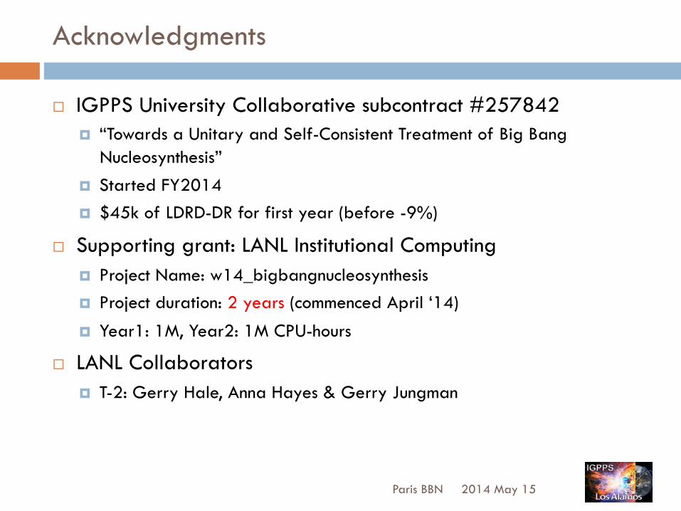
Acknowledgments

¨  IGPPS University Collaborative subcontract #257842 ¤  “Towards a Unitary and Self-Consistent Treatment of Big Bang

Nucleosynthesis” ¤  Started FY2014 ¤  $45k of LDRD-DR for first year (before -9%)

¨  Supporting grant: LANL Institutional Computing ¤  Project Name: w14_bigbangnucleosynthesis ¤  Project duration: 2 years (commenced April ‘14)

¤  Year1: 1M, Year2: 1M CPU-hours

¨  LANL Collaborators ¤  T-2: Gerry Hale, Anna Hayes & Gerry Jungman

2014 May 15 Paris BBN

Supporting activities 2013—2014

¨  Paris – T-2 staff member [Jan. 2012 hire] ¤  International conferences (2 invited, 1 contributed), seminars, workshops ¤  4 peer-review publications on light nuclear reactions ¤  LANL Institutional Computing 2 year grant ¤  LDRD-ER (FY15): BBN proposal oral review 14 May ’14 (yesterday)

¨  Fuller – Director CASS, UCSD ¤  Conferences, colloquia, workshops (many) ¤  Publications (many) ¤  NSF Grant No. PHY- 09-70064 at UCSD

¨  Grohs – Graduate Program UCSD – ABD ¤  15 Feb 2013-Sterile Neutrinos: Dark Matter, Neff, and BBN Implications-CASS

Journal Club-UCSD; 10 Sep 2013-Nucleosynthesis, Neff, and Neutrino Mass Implications from Dark Radiation-NUPAC Seminar-UNM; 13 Jan 2014-Nucleosynthesis, Neff, and Neutrino Mass Implications from Dark Radiation-HEP Seminar-Caltech; 14 Feb 2014-Evidence (to the trained eye) for Sterile Neutrino Dark Matter-CASS Journal Club-UCSD; 28 Mar 2014-Photon Diffusion in the Early Universe-PCGM30 (Pacific Coast Gravity Meeting)-UCSD; 18 Apr 2014-Neutrinos in Cosmology I-CASS Journal Club-UCSD

¤  Dissertation targeted Spring 2015


Organization

Nuclear reactions in the early universe ¨  Lectures (Paris/E. Grohs)

I.  Overview of cosmology/Kinetic theory/Big bang nucleosynthesis (BBN)

II.  Scattering & reaction formalism/Neutrino energy transport

¨  Workshop sessions (E. Grohs/Paris) I.  BBN exercises: compute Nuclear Statistical Equilibrium/electron

fraction II.  Compute primordial abundances vs Ωb h2: code parallelization

¨  Lecture notes ¨  Will be available online (URL TBA)


Possibly useful references


Cosmology notes 33

We might now substitute numerical values into the above expression for the followingquantities:

⇢c = 1.88⇥ 10�29h2 g/cm3, (225)

mN = 1.67⇥ 10�24 g, (226)

�T = 0.665⇥ 10�24 cm2, (227)

H0 = 100h km/s Mpc�1, (228)

c = 2.998⇥ 105 km s�1 (229)

Collecting:

⇢c/h2�TH0/h

mN

=1.88⇥ 10�29 g cm�3

1.67⇥ 10�24 g⇥ 0.665⇥ 10�24 cm2

⇥

102 km s�1 Mpc�1

2.998⇥ 105 km s�1

⇥ 3.1⇥ 1024 cm Mpc�1 (230)

=1

1.29⇥ 108 Mpc2. (231)

Substitution in Eq.(224) gives

a20k�2D (a) = 9.17⇥ 106 Mpc2

n

⌦bh2⇥

1� 12Yp

⇤ ⇥

⌦mh2⇤1/2

o�1

⇥

✓

a

a0

◆5/2n

83

h

�

1 + aeq

a

�5/2�

�aeq

a

�5/2i

�

203

�

1 + aeq

a

�3/2+ 5

�

1 + aeq

a

�1/2o

, (232)

which is pretty close to Evan’s result [Eq.(2)] on his p.15 of Neff v3.1.pdf.

[1] Wikipedia, Recombination (cosmology), http://en.wikipedia.org/wiki/Recombination_(cosmology)#cite_note-1 (2010), [Online; accessed 01 July 2014].

[2] S. Weinberg, Gravitation and Cosmology (John Wiley & Sons, 1972).[3] S. Detweiler, Classical and Quantum Gravity 22, S681 (2005), URL http://stacks.iop.

org/0264-9381/22/i=15/a=006.[4] L. Landau and E. Lifshitz, Mechanics, v. 1 (Elsevier Science, 1982), ISBN 9780080503479,

URL http://books.google.com/books?id=bE-9tUH2J2wC.[5] Planck Collaboration, P. A. R. Ade, N. Aghanim, C. Armitage-Caplan, M. Arnaud, M. Ash-

down, F. Atrio-Barandela, J. Aumont, C. Baccigalupi, A. J. Banday, et al., ArXiv e-prints(2013), 1303.5076.

[6] D. Baumann, ArXiv e-prints (2009), 0907.5424.[7] S. Dodelson, Modern Cosmology, Academic Press (Academic Press, 2003), ISBN

9780122191411, URL http://books.google.com/books?id=3oPRxdXJexcC.[8] P. Ade et al., Phys. Rev. Lett. 112, 241101 (2014).[9] K. Huang, Statistical mechanics (Wiley, 1987), ISBN 9780471815181, URL http://books.

google.com/books?id=M8PvAAAAMAAJ.[10] L. Brown, Quantum Field Theory (Cambridge University Press, 1994), URL http://books.

google.com/books?id=_qt_nQEACAAJ.

Cosmology notes 34

[11] E. Lifshitz and L. Pitaevskiı, Physical Kinetics, no. v. 10 in Course of theoretical physics(Butterworth-Heinemann, 1981), ISBN 9780750626354, URL http://books.google.com/

books?id=h7LgAAAAMAAJ.[12] M. Peskin and D. Schroeder, An Introduction to Quantum Field Theory, Advanced book

classics (Addison-Wesley Publishing Company, 1995).[13] J. Bernstein, Kinetic Theory in the Expanding Universe (Cambridge University Press, 1988).

Outline

Lecture I ¨  Overview

¨  Cosmological dynamics in GR

¨  Big bang nucleosynthesis (BBN)

¨  Boltzmann equation ¤  Flat & curved spacetime

Lecture II

¨  Unitary reaction network (URN) of light nuclei

¨  Neutrino energy transport ¨  Evan Grohs: observations of primordial abundances


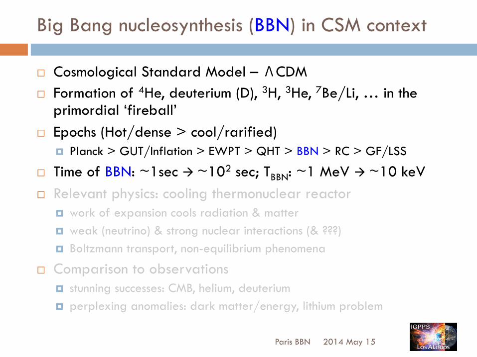
Big Bang nucleosynthesis (BBN) in CSM context

¨  Cosmological Standard Model – ΛCDM ¨  Formation of 4He, deuterium (D), 3H, 3He, 7Be/Li, … in the

primordial ‘fireball’ ¨  Epochs (Hot/dense > cool/rarified)

¤  Planck > GUT/Inflation > EWPT > QHT > BBN > RC > GF/LSS

¨  Time of BBN: ~1sec à ~102 sec; TBBN: ~1 MeV à ~10 keV ¨  Relevant physics: cooling thermonuclear reactor

¤  work of expansion cools radiation & matter ¤  weak (neutrino) & strong nuclear interactions (& ???) ¤  Boltzmann transport, non-equilibrium phenomena

¨  Comparison to observations ¤  stunning successes: CMB, helium, deuterium ¤  perplexing anomalies: dark matter/energy, lithium problem




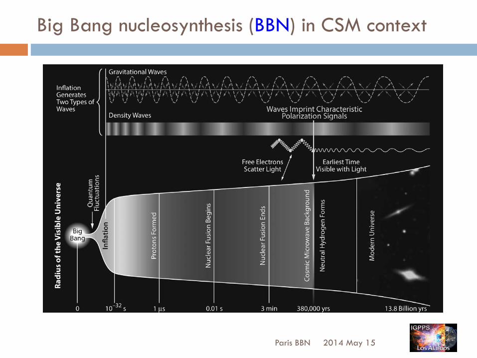
Cosmology notes 15

3 min Time [years] 380,000 13.7 billion10 -34 sRedshift 026251,10010 4

Energy 1 meV1 eV1 MeV10 15 GeV

Scale a(t)

10 -

?

Cosmic Microwave BackgroundLensing

Ia

QSOLy!

gravity wavesB-mode Polarization

21 cm

neutrinos

recombinationBBNreheating

Infla

tion

reionizationgalaxy formation dark energy

LSSBAO

dark ages

density fluctuations

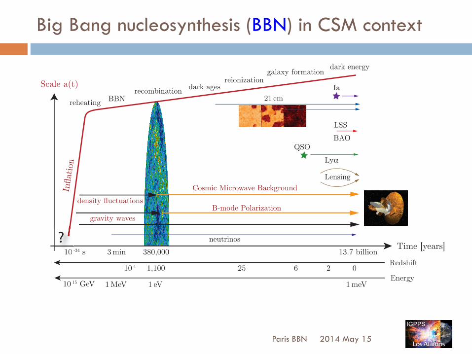
FIG. 1: History of the universe in terms of the major epochs defined variously by properties ofradiation and matter.[6]

where ⇢c,100 is a constant with dimension [⇢c,100] = g/cm3 which gives the value of ⇢c whenH0 = 100 km/s/Mpc. Look up the value of H0 in the abstract of the recent Planck collabo-ration paper[5]. Show that ⇢c,0, in units of the number density of protons, is

⇢c,0 =3

8⇡H2

0m2pl

= 5.1⇥ 10�6cm�3⇡ 5 m�3. (100)

Before we turn to the explicit solution of the Friedmann equations we’ll need to talkabout the radiation and matter content of the universe, which we do in the next sectionwhere we study their role in equilibrium and non-equilibrium situations.

III. KINETIC THEORY IN CURVED (FRIEDMANN) SPACETIME

The kinetic theory of coupled radiation and matter is an essential component to under-standing basic features of the dynamics of the early, hot universe. Figure 1 gives an overviewof the major epochs in the evolution of the universe in terms of the temperature, T (in energyunits) and the redshift z > 1:

1 + z =a

a0=

�(a0)

�(a), (101)

where �(a) is the wavelength of a photon when the scale factor is a; for distant sourcesthe emission of a photon with wavelength �(a) is shorter than the wavelength when it is


¨  Cosmological Standard Model – ΛCDM ¨  Formation of 4He, deuterium (D), 3H, 3He, 7Be/Li, … in the

primordial ‘fireball’ ¨  Epochs (Hot/dense > cool/rarified)

¤  Planck > GUT/Inflation > EWPT > QHT > BBN > RC > GF/LSS ¨  Time of BBN: ~1sec à ~102 sec; TBBN: ~1 MeV à ~10 keV ¨  Relevant physics: cooling thermonuclear reactor

¤  work of expansion cools radiation & matter ¤  weak (neutrino) & strong nuclear interactions (& ???) ¤  Boltzmann transport, non-equilibrium phenomena

¨  Comparison to observations ¤  stunning successes: CMB, helium, deuterium ¤  perplexing anomalies: dark matter/energy, lithium problem


Observations [more from Evan G. tomorrow]

!! Observational astronomy !! existing 10m-class telescopes: Keck, …

#! Gold-plated: 2% D meas. Pettini & Cooke ‘13 !! adaptive optics !! space- & ground-based observatories

!! planned 30+m-class telescopes: ELT, TMT, …

!! Cosmic microwave background !! Planck, WMAP, PolarBear, APT, SPT, CMBPol, …

!! Implications !! test physics beyond SM; lab tests difficult/impossible

!! precision constraints expected to test nuclear physics

!! Unprecedented precision for primordial nuclear abundances


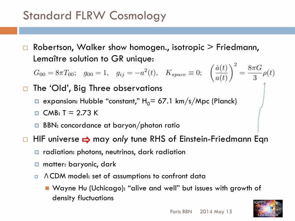
Standard FLRW Cosmology

¨  Robertson, Walker show homogen., isotropic > Friedmann, Lemaître solution to GR unique:

¨  The ‘Old’, Big Three observations ¤  expansion: Hubble “constant,” H0= 67.1 km/s/Mpc (Planck) ¤  CMB: T = 2.73 K

¤  BBN: concordance at baryon/photon ratio

¨  HIF universe may only tune RHS of Einstein-Friedmann Eqn ¤  radiation: photons, neutrinos, dark radiation

¤  matter: baryonic, dark ¤  ΛCDM model: set of assumptions to confront data

n  Wayne Hu (Uchicago): “alive and well” but issues with growth of density fluctuations


G00 = 8⇡T00; g00 = 1, gij = �a2(t), Kspace ⌘ 0;

✓a(t)

a(t)

◆2

=8⇡G

3⇢(t)

Einstein-Friedmann equations (0)


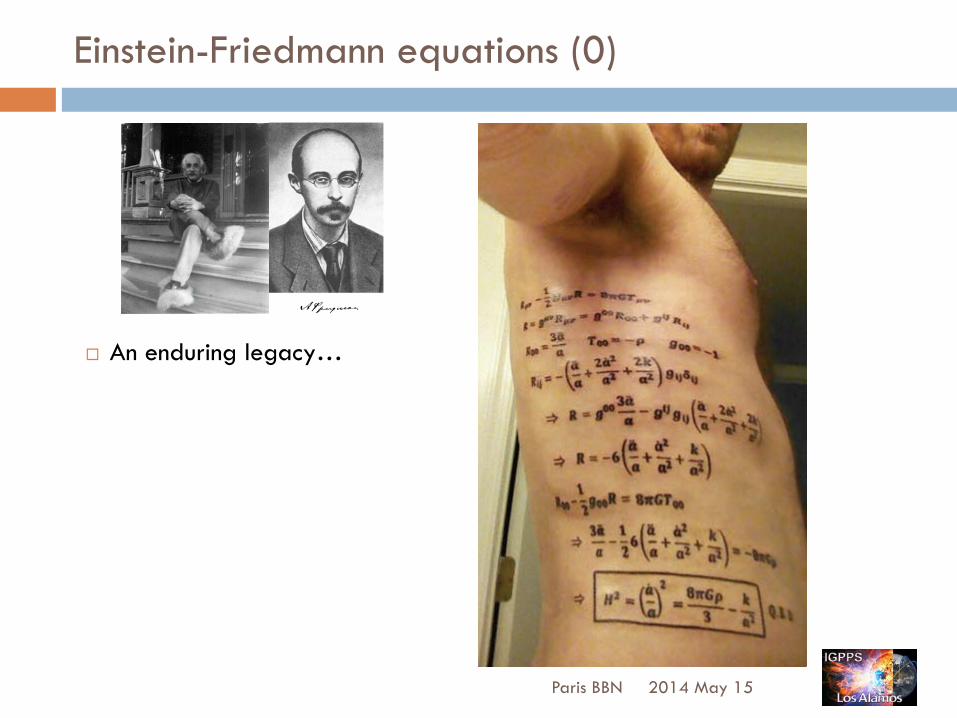
!! An enduring legacy…

Einstein-Friedmann equations (I)

¨  Universe dynamics from GR energy-momentum density


Gµ⌫ = 8⇡Tµ⌫

Tµ⌫ = �pgµ⌫ + (p+ ⇢)uµu⌫

g00 = 1, gij = a2(t)gijGµ⌫ = Rµ⌫ � 1

2gµ⌫R

Rµ⌫ = g

↵�R↵µ�⌫ = R

�µ�⌫ = R

↵↵µ ⌫

R = g

µ⌫Rµ⌫

R

µ⌫⇢� =

@�µ⌫�

@x

⇢�

@�µ⌫⇢

@x

�

+ �⌧⌫��

µ⇢⌧ � �⌧

⌫⇢�µ

�⌧

¨  Einstein/Ricci/Curv Scalar ¨  Metric/connection Cosmology notes 10

This gives for the components of the connection:

�000 =

12g

0↵(2g↵0,0 � g00,↵) = 0 (65)

�0i0 =

12g

0↵(g↵i,0 + g↵0,i � gi0,↵) = 0 (66)

�0ij =

12g

0↵(g↵i,j + g↵j,i � gij,↵) = �

12gij,0 = �aagij (67)

�i00 =

12g

i↵(2g↵0,0 � g00,↵) = 0 (68)

�ij0 =

12g

i↵g↵j,0 =12

1

a2gik

@[a2gkj]

@x0=

a

a�ij = �i

0j (69)

�ijk =

12 g

il(glj,k + glk,j � gjk,l) ⌘ �ijk. (70)

Equipped with the components of the connection, �ijk of the FLRW metric, we can

consider the equation of motion of objects in free-fall – the geodesic equation [Eq.(41)]:

x⇢ + �⇢µ⌫ x

µx⌫ = 0. (41)

Consider the ⇢ = 0 (time) component:

d2x0

d⌧ 2+ �0

µ⌫ xµx⌫ =

d2x0

d⌧ 2�H(t)(ax)2 = 0. (71)

Here, we have defined the Hubble parameter

H(t) =a(t)

a(t). (72)

It is generally a function of t (the ‘Hubble constant’, H0 is the value of the Hubble parameternow). According to Eq.(71), particles at rest with respect to the cosmological coordinates,x = 0 have

x0 = !⌧ � ⌧0, (73)

where ! = dx0/d⌧ |⌧0 and ⌧0 are constants that set the rate and zero of universal time.“Clocks” have ! = 1 and we may take ⌧0 = 0 to coincide with the big bang (see below,Subsec.IID, on the Friedmann evolution equation).

Exercise 7. Use the ⇢ = 0 component of Eq.(41) to compute the spatial components of thegeodesic for particles at rest with respect to the cosmological coordinates.

Einstein-Friedmann equations (II)

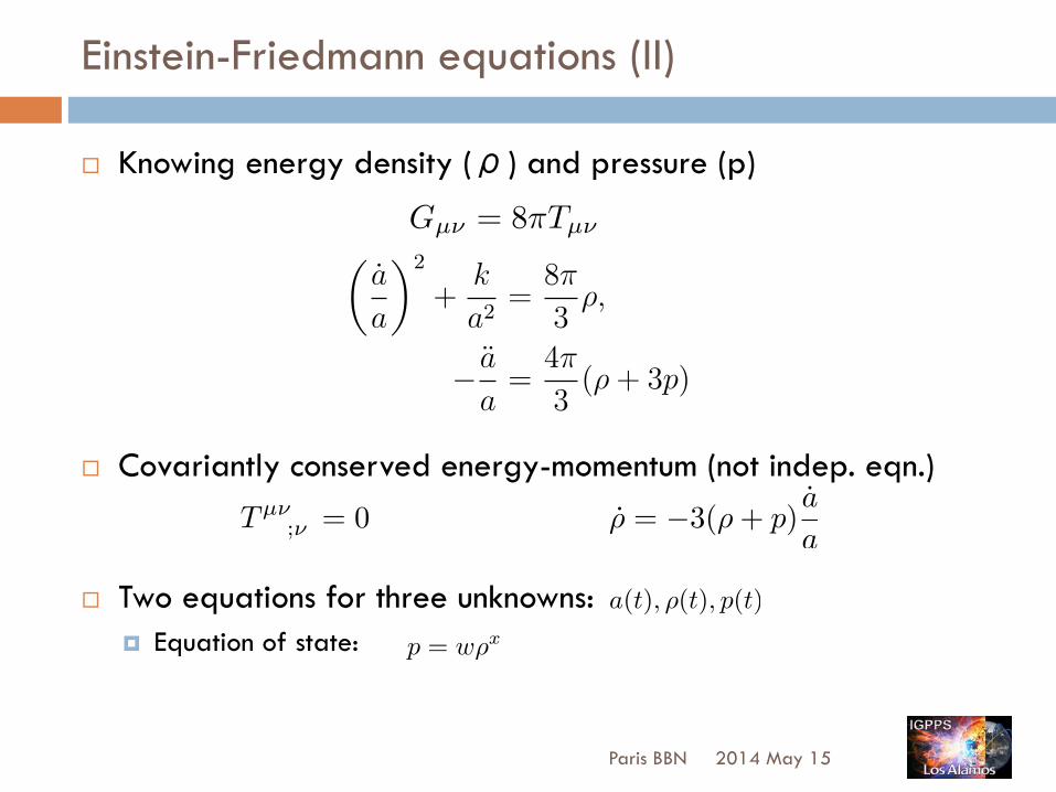
¨  Knowing energy density (ρ) and pressure (p)


Gµ⌫ = 8⇡Tµ⌫

Cosmology notes 13

Collecting this relation with Eq.(87) gives

✓

a

a

◆2

+k

a2=

8⇡

3⇢, (90)

�

a

a=

4⇡

3(⇢+ 3p), (91)

the usual form quoted for the Friedmann equations. Due to the fact that the first equationabove is an (non-linear) ordinary di↵erential equation of first-order in time and that thesecond equation is second-order, there is a consistency condition that arises if we di↵erentiatethe first equation once:

⇢ = �3(⇢+ p)a

a. (92)

Note that we have two equations here for three unknowns, a(t), ⇢(t), p(t) since this equationis a consequence of the Friedmann equations. In fact, Eq.(92) arises from the fact that theenergy-momentum tensor is covariantly conserved:

T µ⌫;⌫ = 0, (93)

a consequence of the identity Gµ⌫;⌫ = 0. So the conservation equation doesn’t close the

system of equations for (a, ⇢, p). It’s a general feature of GR that the conservation of four-momentum is a consequence of the geometric structure of the theory as encoded in theEinstein tensor. If we assume that we know the equation of state p = p(⇢), which we do fornon-interacting, non-relativistic matter and for radiation, then we may determine a solutionfor the Friedmann equations.

Exercise 9. Show that Eq.(92) is a consequence of Eq.(93).

Let’s assume for the sake of simplicity that the equation of state exists and is given by asimple power law in the energy density:

p = c⇢x, (94)

where c > 0 is a constant. This relation is similar to the polytropic equation of state.

Exercise 10. Use Eq.(92) to show that the expression for ⇢(a) is given as

⇢(a) =

8

>

<

>

:

⇣

⇢(a0)�

a0a

�3⌘1�x

+ c⇣

�

a0a

�3(1�x)� 1

⌘

�

11�x

, x 6= 1,

⇢(a0)3c

�

a0a

�4, x = 1.

(95)

Here, a0 is some reference scale factor with a0 > a, usually taken to be the scale factor now.Consider the cases: i) c = 0 (pressureless dust); ii) x = 1, c = 1

3 (radiation); iii) x = 1,c = �1 (dark energy) (Hint: go back to Eq.(92) for this part.)

Tµ⌫;⌫ = 0 ⇢ = �3(⇢+ p)

a

a

¨  Covariantly conserved energy-momentum (not indep. eqn.)

¨  Two equations for three unknowns: ¤  Equation of state:

a(t), ⇢(t), p(t)

p = w⇢x

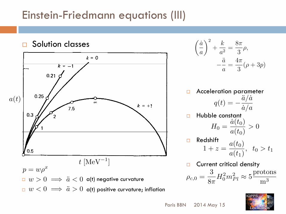
¨  Acceleration parameter

¨  Hubble constant

¨  Redshift

¨  Current critical density

Einstein-Friedmann equations (III)

¨  Solution classes


a(t)q(t) = � a/a

a/a

Cosmology notes 13

Collecting this relation with Eq.(87) gives

✓

a

a

◆2

+k

a2=

8⇡

3⇢, (90)

�

a

a=

4⇡

3(⇢+ 3p), (91)

the usual form quoted for the Friedmann equations. Due to the fact that the first equationabove is an (non-linear) ordinary di↵erential equation of first-order in time and that thesecond equation is second-order, there is a consistency condition that arises if we di↵erentiatethe first equation once:

⇢ = �3(⇢+ p)a

a. (92)

Note that we have two equations here for three unknowns, a(t), ⇢(t), p(t) since this equationis a consequence of the Friedmann equations. In fact, Eq.(92) arises from the fact that theenergy-momentum tensor is covariantly conserved:

T µ⌫;⌫ = 0, (93)

a consequence of the identity Gµ⌫;⌫ = 0. So the conservation equation doesn’t close the

system of equations for (a, ⇢, p). It’s a general feature of GR that the conservation of four-momentum is a consequence of the geometric structure of the theory as encoded in theEinstein tensor. If we assume that we know the equation of state p = p(⇢), which we do fornon-interacting, non-relativistic matter and for radiation, then we may determine a solutionfor the Friedmann equations.

Exercise 9. Show that Eq.(92) is a consequence of Eq.(93).

Let’s assume for the sake of simplicity that the equation of state exists and is given by asimple power law in the energy density:

p = c⇢x, (94)

where c > 0 is a constant. This relation is similar to the polytropic equation of state.

Exercise 10. Use Eq.(92) to show that the expression for ⇢(a) is given as

⇢(a) =

8

>

<

>

:

⇣

⇢(a0)�

a0a

�3⌘1�x

+ c⇣

�

a0a

�3(1�x)� 1

⌘

�

11�x

, x 6= 1,

⇢(a0)3c

�

a0a

�4, x = 1.

(95)

Here, a0 is some reference scale factor with a0 > a, usually taken to be the scale factor now.Consider the cases: i) c = 0 (pressureless dust); ii) x = 1, c = 1

3 (radiation); iii) x = 1,c = �1 (dark energy) (Hint: go back to Eq.(92) for this part.)

p = w⇢x

¨  a(t) negative curvature

¨  a(t) positive curvature; inflation

w > 0 =) a < 0

w < 0 =) a > 0

1 + z =a(t0)

a(t1), t0 > t1

H0 =a(t0)

a(t0)> 0

⇢c,0 =

3

8⇡H2

0m2Pl ⇡ 5

protons

m

3

t [MeV�1]

Einstein-Friedmann equations (IV)

¨  Maximally symmetric subspace ¤  Consequence of homogeneity & isotropy

¤  ‘Maximal’ number L.I. Killing vector fields N(N+1)/2 (dim N) ¤  Flows of Killing vector fields generate isometries of manifold

¤  Friedman universe has MS spacelike hypersurfaces

¨  Tensors in MS spaces ¤  scalar:

¤  vector:

¤  rank-2 tensor:


@µS(x) = 0

A

i(x) ⌘ 0 (A0(x) 6= 0)

Bij = Bji = Cgij C 6= C(x)

Standard BBN – 7Li anomaly

3He/H p

4He

2 3 4 5 6 7 8 9 101

0.01 0.02 0.030.005

CM

B

BB

N

Baryon-to-photon ratio ! " 1010

Baryon density #bh2

D___H

0.24

0.23

0.25

0.26

0.27

10$4

10$3

10$5

10$9

10$10

2

57Li/H p

Yp

D/H p

Figure 20.1: The abundances of 4He, D, 3He, and 7Li as


¨  n/p ratio ¤  exquisite sensitivity to neutrino distribution

¤  ~1:5

¨  Helium ¤  exquisite sensitivity to neutrons

¤  mass fraction Yp~1/4 (p:primordial)

¨  Deuterium ¤  ~1:105

¤  Pettini & Cooke obs. better by fact 5

¨  Lithium ¤  mass A=7

n  3—5σ discrepancy > Li anomaly Review Particle Properties

Workshop II: generate ‘Schramm plot’

h=H0/(100 km/s/Mpc)

The New, ‘Big Five’ observations

¨  comprehensive cosmic microwave background (CMB) observations (WMAP, Planck, ACT, SPT, PolarBear, CMBPol,...) ¤  Neff : “effective number” of relativistic species;Yp : 4He mass fraction

(relative to proton);η(Ωb): baryon-to-photon number fraction; Primordial deuterium abundance (D/H)p;Σmν

¨  10/30-meter class telescopes, adaptive optics, and orbiting observatories ¤  e.g., precision determinations of deuterium abundance dark energy/

matter content, structure history etc.

¨  Laboratory neutrino mass/mixing measurements ¤  mini/micro-BooNE, EXO, LBNE


GF: “VERY EXCITING situa&on developing . . . because of the advent of . . .”

GF: “is se6ng up a nearly over-‐determined situa>on where new Beyond Standard Model neutrino physics likely must show itself!”

ΛCDM: Possible discrepancies (I)

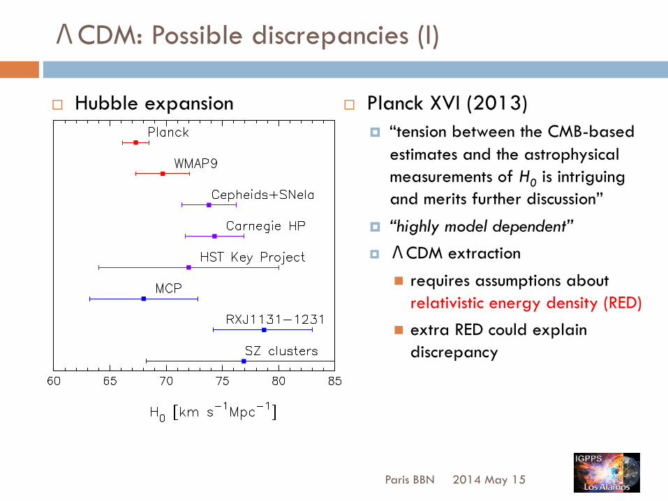
¨  Hubble expansion


Planck Collaboration: Cosmological parameters

Fig. 16. Comparison of H0 measurements, with estimates of±1� errors, from a number of techniques (see text for details).These are compared with the spatially-flat ⇤CDM model con-straints from Planck and WMAP-9.

excellent agreement with the base ⇤CDM model evident in Fig.15, we can infer that the combination of Planck and BAO mea-surements will lead to tight constraints favouring ⌦K = 0 (Sect.6.2) and a dark energy equation-of-state parameter, w = �1(Sect. 6.5). Since the BAO measurements are primarily geomet-rical, they are used in preference to more complex astrophysicaldatasets to break CMB parameter degeneracies in this paper.

Finally, we note that we choose to use the6dF+SDSS(R)+BOSS data combination in the likelihoodanalysis of Sect. 6. This choice includes the two most accu-rate BAO measurements and, since the e↵ective redshifts ofthese samples are widely separated, it should be a very goodapproximation to neglect correlations between the surveys.

5.3. The Hubble constant

A striking result from the fits of the base⇤CDM model to Planckpower spectra is the low value of the Hubble constant, which istightly constrained by CMB data alone in this model. From thePlanck+WP+highL analysis we find

H0 = (67.3±1.2) km s�1 Mpc�1 (68%; Planck+WP+highL).(51)

A low value of H0 has been found in other CMB experi-ments, most notably from the recent WMAP-9 analysis. Fittingthe base ⇤CDM model, Hinshaw et al. (2012) find24

H0 = (70.0 ± 2.2) km s�1 Mpc�1 (68%; WMAP-9), (52)

consistent with Eq. (51) to within 1�. We emphasize here thatthe CMB estimates are highly model dependent. It is importanttherefore to compare with astrophysical measurements of H0,since any discrepancies could be a pointer to new physics.

24The quoted WMAP-9 result does not include the 0.06 eV neutrinomass of our base ⇤CDM model. Including this mass, we find H0 =(69.7 ± 2.2) km s�1 Mpc�1 from the WMAP-9 likelihood.

There have been remarkable improvements in the preci-sion of the cosmic distance scale in the last decade or so.The final results of the Hubble Space Telescope (HST) KeyProject (Freedman et al. 2001), which used Cepheid calibrationsof secondary distance indicators, resulted in a Hubble constantof H0 = (72 ± 8) km s�1 Mpc�1 (where the error includes esti-mates of both 1� random and systematic errors). This estimatehas been used widely in combination with CMB observationsand other cosmological data sets to constrain cosmological pa-rameters (e.g., Spergel et al. 2003, 2007). It has also been recog-nized that an accurate measurement of H0 with around 1% pre-cision, when combined with CMB and other cosmological data,has the potential to reveal exotic new physics, for example, atime-varying dark energy equation of state, additional relativisticparticles, or neutrino masses (see e.g., Suyu et al. 2012, and ref-erences therein). Establishing a more accurate cosmic distancescale is, of course, an important problem in its own right. Thepossibility of uncovering new fundamental physics provides anadditional incentive.

Two recent analyses have greatly improved the precision ofthe cosmic distance scale. Riess et al. (2011) use HST observa-tions of Cepheid variables in the host galaxies of eight SNe Ia tocalibrate the supernova magnitude-redshift relation. Their “bestestimate” of the Hubble constant, from fitting the calibrated SNemagnitude-redshift relation, is

H0 = (73.8 ± 2.4) km s�1 Mpc�1 (Cepheids+SNe Ia), (53)

where the error is 1� and includes known sources of systematicerrors. At face value, this measurement is discrepant with thePlanck estimate in Eq. (51) at about the 2.5� level.

Freedman et al. (2012), as part of the Carnegie HubbleProgram, use Spitzer Space Telescope mid-infrared observationsto recalibrate secondary distance methods used in the HST KeyProject. These authors find

H0 = [74.3 ± 1.5 (statistical) ± 2.1 (systematic)] km s�1 Mpc�1

(Carnegie HP). (54)

We have added the two sources of error in quadrature in theerror range shown in Fig. 16. This estimate agrees well withEq. (53) and is also discordant with the Planck value (Eq. 16)at about the 2.5� level. The error analysis in Eq. (54) does notinclude a number of known sources of systematic error and isvery likely an underestimate. For this reason, and because of therelatively good agreement between Eqs. (53) and (54), we do notuse the estimate in Eq. (54) in the likelihood analyses describedin Sect. 6.

The dominant source of error in the estimate in Eq. (53)comes from the first rung in the distance ladder. Using themegamaser-based distance to NGC4258, Riess et al. (2011) find(74.8±3.1) km s�1 Mpc�1.25 Using parallax measurements for 10Milky Way Cepheids, they find (75.7 ± 2.6) km s�1 Mpc�1, andusing Cepheid observations and a revised distance to the LargeMagellanic Cloud, they find (71.3 ± 3.8) km s�1 Mpc�1. Theseestimates are consistent with each other, and the combined esti-mate in Eq. (53) uses all three calibrations. The fact that the er-ror budget of measurement (53) is dominated by the “first-rung”calibrators is a point of concern. A mild underestimate of the

25 As noted in Sect. 1, after the submission of this paperHumphreys et al. (2013) reported a new geometric maser distanceto NGC4258 that leads to a reduction of the Riess et al. (2011)NGC4258 value of H0 from (74.8 ± 3.1) km s�1 Mpc�1 to H0 = (72.0 ±3.0) km s�1 Mpc�1.

32

¨  Planck XVI (2013) ¤  “tension between the CMB-based

estimates and the astrophysical measurements of H0 is intriguing and merits further discussion”

¤  “highly model dependent” ¤  ΛCDM extraction

n  requires assumptions about relativistic energy density (RED)

n  extra RED could explain discrepancy

ΛCDM: Possible discrepancies (II)

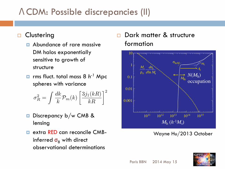
¨  Dark matter & structure formation


¨  Clustering ¤  Abundance of rare massive

DM halos exponentially sensitive to growth of structure

¤  rms fluct. total mass 8 h-1 Mpc spheres with variance

¤  Discrepancy b/w CMB & lensing

¤  extra RED can reconcile CMB-inferred σ8 with direct observational determinations

0.001

0.01

0.1

1

10

1011 1012 1013 1014 1015

M*!0

dnh

d lnMh

msAs

Mth

"lnM

Mh (h-1M )

N(Mh)occupation

�2R =

Zdk

kPm(k)

3j1(kR)

kR

�2

Wayne Hu/2013 October

CDM: Possible discrepancies (III)

!! Big Bang nucleosynthesis !! Lithium anomaly

!! YP,YDP exquisite sensitivity to active neutrino spectrum: #! Most neutrons " 4He #! Yp $ n/p $ f (p,T)

!! Thermal effects #! Hotter later: less neutrons #! Non-equilibrium : less

neutrons !! Probe neutrino sector by

studying constraints on various scenarios imposed by precision BBN


Planck XVI (2013) Planck XVI (2013)

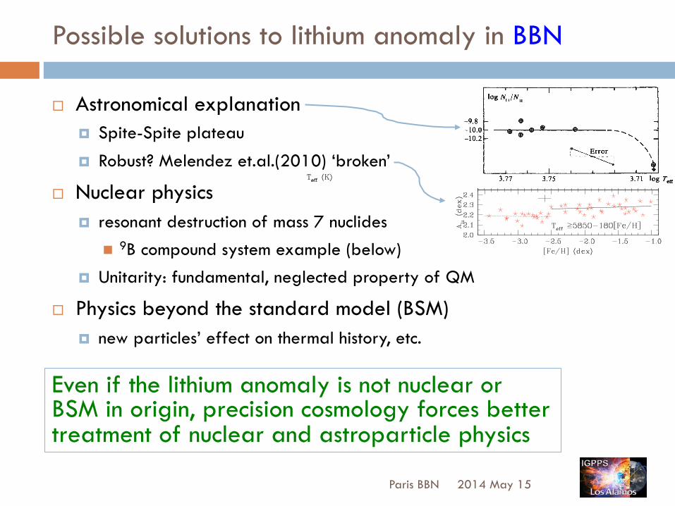
Possible solutions to lithium anomaly in BBN

¨  Astronomical explanation ¤  Spite-Spite plateau

¤  Robust? Melendez et.al.(2010) ‘broken’

¨  Nuclear physics ¤  resonant destruction of mass 7 nuclides

n  9B compound system example (below) ¤  Unitarity: fundamental, neglected property of QM

¨  Physics beyond the standard model (BSM) ¤  new particles’ effect on thermal history, etc.


© Nature Publishing Group1982

J. Meléndez et al.: Li depletion in Spite plateau stars

Fig. 2. Li abundances vs. Te! for our sample stars in di!erent metallicityranges. A typical error bar is shown.

work is that now we select stars with errors in EW below5% (typically !2"3%), instead of the 10% limit adopted inMR04. The only exceptions are the cool dwarfs HD 64090and BD+38 4955, which are severely depleted in Li and haveEW errors of 8% and 10%, respectively, and the very metal-poorstars (B07) BPS CS29518-0020 (5.2%) and BPS CS29518-0043(6.4%), which were kept due to their low metallicity.

The main sources of error are the uncertainties in equiv-alent widths and Te! , which in our work have typical val-ues of only 2.3% and 50 K, implying abundance errors of0.010 dex and 0.034 dex, respectively, and a total error in ALiof !0.035 dex. This low error in ALi is confirmed by the star-to-star scatter of the Li plateau stars, which have similar low values(e.g. ! = 0.036 dex for [Fe/H] < "2.5, see below). Our Li abun-dances and stellar parameters are given in Table 1 (available inthe online edition).

4. Discussion

4.1. The Te! cutoff of the Spite plateau

Despite the fact that Li depletion depends on mass(e.g. Pinsonneault et al. 1992), this variable has been ig-nored by most previous studies. Usually a cuto! in Te! isimposed to exclude severely Li-depleted stars in the Spiteplateau, with a wide range of adopted cuto!s, such as 5500 K(Spite & Spite 1982), 5700 K (B05), 6000 K (MR04; S07) and!6100 K for stars with [Fe/H] < "2.5 (Hosford et al. 2009).

At a given mass, the Te! of metal-poor stars has a strongmetallicity-dependence (e.g. Demarque et al. 2004). As shownin Figs. 11, 12 of M06, the Te! of turno! stars increases for de-creasing metallicities. Hence, a metallicity-independent cuto! inTe! may be an inadequate way to exclude low-mass Li-depletedstars from the Spite plateau. As show in Fig. 2, where ALi in dif-ferent metallicity bins is shown as a function of Te!, stars withlower Te! in a given metallicity regime are typically the starswith the lowest Li abundances, an e!ect that can be seen evenin the sample stars with the lowest metallicities ([Fe/H] ! "3).This is ultimately so because the coolest stars are typically theleast massive, and therefore have been more depleted in Li(see Sect. 4.3).

In Fig. 3 we show the Li abundance for cuto!s =5700 K(open circles), 6100 K (filled squares) and 6350 K (filled tri-angles). Using a hotter cuto! is useful to eliminate the mostLi-depleted stars at low metallicities, but it removes from theSpite plateau stars with [Fe/H] > "2. Imposing a hotter Te! cut-o! at low metallicities and a cooler cuto! at high metallicitieseliminates the most Li-depleted stars at low metallicities, but

Fig. 3. Li abundances for stars with Te! > 5700 K (open circles),>6100 K (filled squares), >6350 K (filled triangles) and #5850"180 $[Fe/H] (stars). In the bottom panel stars above the cuto! in Te! fall intotwo flat plateaus with ! = 0.04 and 0.05 dex for [Fe/H] < "2.5 (dottedline) and [Fe/H] # "2.5 (solid line), respectively.

keeps the most metal-rich stars in the Spite plateau. We proposesuch a metallicity-dependent cuto! below.

4.2. Two flat Spite plateaus

Giving the shortcomings of a constant Te! cuto!, we propose anempirical cuto! of Te! = 5850"180 $ [Fe/H]. The stars abovethis cuto! are shown as stars in the bottom panel of Fig. 3.Our empirical cuto! excludes only the most severely Li-depletedstars, i.e., the stars that remain in the Spite plateau may stillbe a!ected by depletion. The less Li-depleted stars in the bot-tom panel of Fig. 3 show two well-defined groups separated at[Fe/H] ! "2.5 (as shown below, this break represents a real dis-continuity), which have essentially zero slopes (within the errorbars) and very low star-to-star scatter in their Li abundances.The first group has "2.5 % [Fe/H] < "1.0 and &ALi'1 = 2.272(! = 0.051) dex and a slope of 0.018 ± 0.026, i.e., flatwithin the uncertainties. The second group is more metal poor([Fe/H] < "2.5) and has &ALi'2 = 2.184 dex (! = 0.036) dex.The slope of this second group is also zero ("0.008 ± 0.037).Adopting a more conservative exponential cuto! obtained fromY2 isochrones (Demarque et al. 2004), which for a 0.79 M( starcan be fit by Te! = 6698"2173 $ e[Fe/H]/1.021, we would also re-cover a flat Spite plateau, although only stars with [Fe/H] > "2.5are left using this more restrictive cut-o!. Thus, the flatness ofthe Spite plateau is independent of applying a linear or an expo-nential cuto!.

Adopting a constant cuto! in Te! we also find flat plateaus.For example adopting a cuto! of Te! > 6100 K (filled squares inFig. 3) we find in the most metal-rich plateau ([Fe/H] # "2.5)no trend between Li and [Fe/H] (slope = 0.019 ± 0.025,Spearman rank correlation coe"cient rSpearman = 0.1 and a prob-ability of 0.48 (i.e., 48%) of a correlation arising by pure chancefor [Fe/H] # "2.5), while for the most metal-poor plateau([Fe/H] < "2.5) we also do not find any trend within theerrors (slope = 0.058 ± 0.072, rSpearman = 0.2 and 41%probability of a spurious correlation). Using a hotter cuto!(Te! > 6350 K, filled triangles in Fig. 3) we obtain also two flat

Page 3 of 7

Even if the lithium anomaly is not nuclear or BSM in origin, precision cosmology forces better treatment of nuclear and astroparticle physics

Possible refinements to BBN

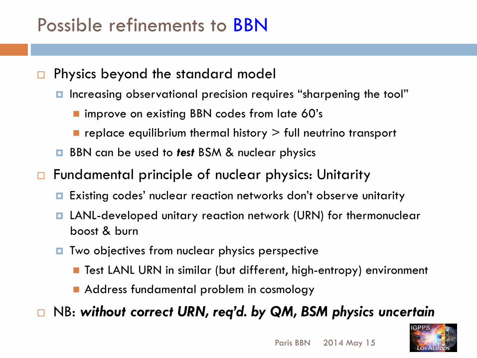
¨  Physics beyond the standard model ¤  Increasing observational precision requires “sharpening the tool”

n  improve on existing BBN codes from late 60’s n  replace equilibrium thermal history > full neutrino transport

¤  BBN can be used to test BSM & nuclear physics

¨  Fundamental principle of nuclear physics: Unitarity ¤  Existing codes’ nuclear reaction networks don’t observe unitarity

¤  LANL-developed unitary reaction network (URN) for thermonuclear boost & burn

¤  Two objectives from nuclear physics perspective n  Test LANL URN in similar (but different, high-entropy) environment n  Address fundamental problem in cosmology

¨  NB: without correct URN, req’d. by QM, BSM physics uncertain


BBN project: introduce a new theoretical tool

¨  Outline for the rest of talk ¤  1st refinement: neutrino sector

¤  2nd refinement: nuclear physics


BBN project: introduce a new theoretical tool

!! Outline for the rest of talk !! 1st refinement: neutrino sector

!! 2nd refinement: nuclear physics


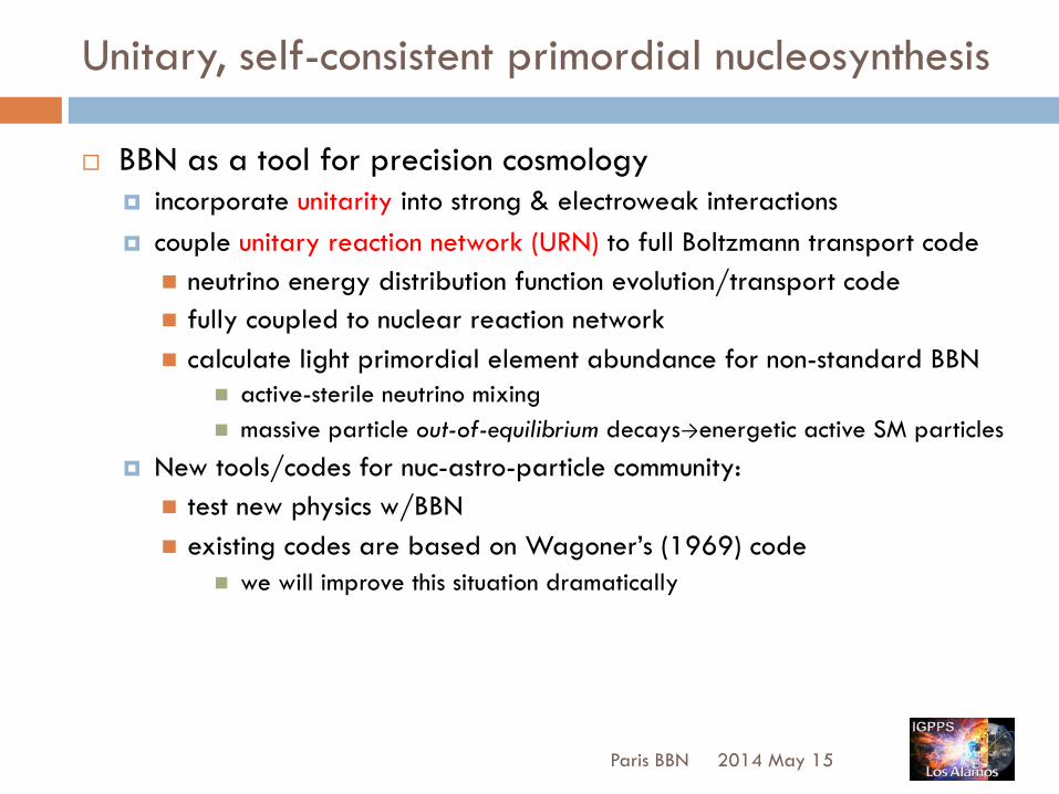
Unitary, self-consistent primordial nucleosynthesis

¨  BBN as a tool for precision cosmology ¤  incorporate unitarity into strong & electroweak interactions ¤  couple unitary reaction network (URN) to full Boltzmann transport code

n  neutrino energy distribution function evolution/transport code n  fully coupled to nuclear reaction network n  calculate light primordial element abundance for non-standard BBN

n  active-sterile neutrino mixing n  massive particle out-of-equilibrium decays→energetic active SM particles

¤  New tools/codes for nuc-astro-particle community: n  test new physics w/BBN n  existing codes are based on Wagoner’s (1969) code

n  we will improve this situation dramatically


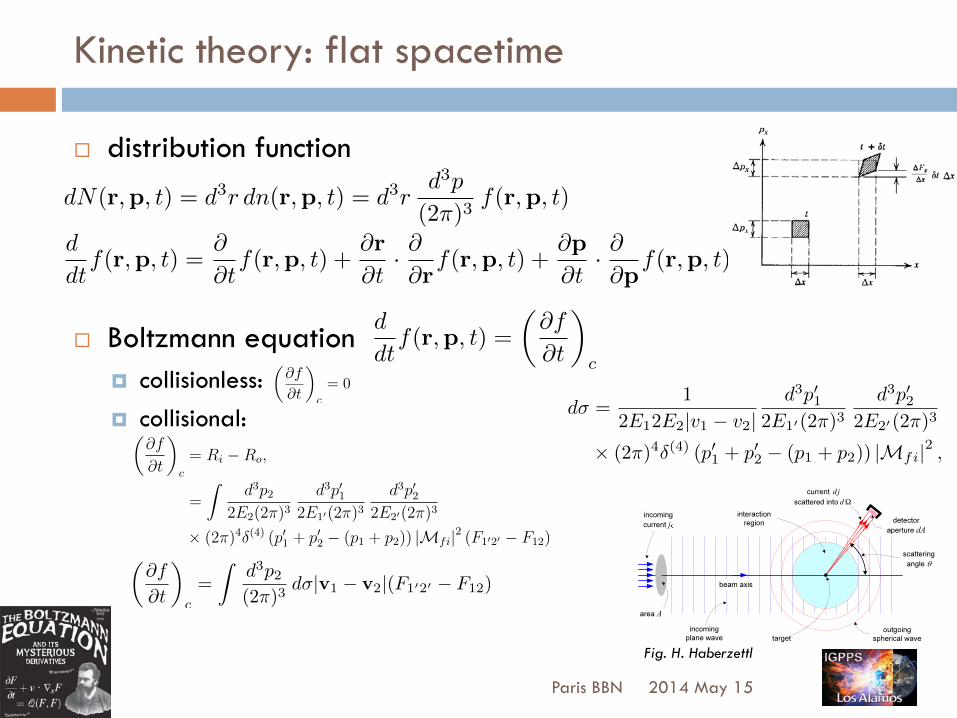
Kinetic theory: flat spacetime

!! distribution function

!! Boltzmann equation !! collisionless: !! collisional:


dN(r,p, t) = d3r dn(r,p, t) = d3rd3p

(2⇡)3f(r,p, t)

d

dtf(r,p, t) =

@

@tf(r,p, t) +

@r

@t· @@r

f(r,p, t) +@p

@t· @@p

f(r,p, t)

d

dtf(r,p, t) =

✓@f

@t

◆

c✓@f

@t

◆

c

= 0

Cosmology notes 21

The collision integral is defined as the di↵erence of these two rates✓

@f

@t

◆

c

= Ri �Ro, (127)

=

Z

d3p22E2(2⇡)3

d3p012E10(2⇡)3

d3p022E20(2⇡)3

⇥ (2⇡)4�(4) (p01 + p02 � (p1 + p2)) |Mfi|2 (F1020 � F12) . (128)

Considering the factors from left to right, we first encounter the integral over the the mo-mentum of the projectile, particle ‘2’, which is required since we consider that a particlewith any initial momentum impinging upon the target is capable of scattering it from itsPSE. The next two integration measures is the final state of the two-body system; no matterthe final state, if a collision has taken place we consider that the target has been removedfrom its the PSE.

The �(4) function enforces conservation of four-momentum. It ensures, among others,that if the incoming energy isn’t su�cient to create the masses of the final state particles,then it sets the integrand to zero. The following factor, |Mfi|

2 is the modulus-squared of thetransition matrix element to go from the initial state |ii = |12i to the final state |fi = |1020ior from |1020i ! |12i. The amplitude is the same for these two processes if the interactionsrespect time reversal invariance and parity conservation: Mfi = Mif .

The last factor takes into account the occupation of the initial and final states. It isthe di↵erence of two correlation functions, each of which is the product of three factors:the two-particle correlation function for particles (1020) in the initial state multiplied byPauli-blocking (Einstein-enhancing) factors for FD (BE) particles in the final state:

F1020 = F (r,p10 ,p20 , t)(1± f(r,p1, t))(1± f(r,p2, t)), (129)

F12 = F (r,p1,p2, t)(1± f(r,p10 , t))(1± f(r,p20 , t)). (130)

The correlation function on the first line, F1020 is for particles scattering into the PSE,while F12 is for particles scattering out of the element. In fact, we adopt the assumption of“molecular chaos” and neglect two-body correlations in the initial states, giving, for example

F12 ⇡ f(r,p1, t)f(r,p2, t). (131)

The definition of the di↵erential scattering cross section for the process 12 ! 1020 is[12]

d� =1

2E12E2|v1 � v2|

d3p012E10(2⇡)3

d3p022E20(2⇡)3

⇥ (2⇡)4�(4) (p01 + p02 � (p1 + p2)) |Mfi|2 , (132)

which upon substitution into Eq.(127) gives

✓

@f

@t

◆

c

= 2E1

Z

d3p2(2⇡)3

|v1 � v2|d�(F1020 � F12) (133)

We have been so far been considering a single species’ distribution function, f in thepreceding. When multiple species are present the distribution functions are adorned witha subscript, fi to denote which particle is being tracked and, possibly, includes informationabout its internal state, which may be written in terms of its quantum numbers.

� � � � � � � � �

� � � � � �

� � � � � � � � �

� � � � � � � � � �

� � � � � � �

� � � �

� � � � � � � � � �

� � � �

� � � � � � � � �

� � � � � � � � �

� � � � �

!

� � � � � � � � � � �

� � � � � �

� � � � � � � � � � �

� � � � � � � � � � � � � � �

djd"

� � � � � � � � �

� � � � � � � � � �

Figure 7.1: Schematic description of the quantum-mechanical scatteringprocess. Part of the incident particle current j0 through the cross-sectionalarea A is scattered under the angle ! with respect to the beam axis. Thecorresponding current scattered into the solid-angle aperture d! of the detec-tor is dj. The asymptotic picture of the scattering process (i.e., the pictureoutside of the interaction region) is that of an incoming plane wave and anoutgoing spherical wave that carries the scattering information to the detec-tor. Assuming a spherically symmetric interaction, this process is cylindricallysymmetric about the beam axis.

The direction of the incoming beam along p is, by convention, takenas the positive z-axis with the target position de� ning the coordinateorigin, z = 0.

We consider here only central forces. The original spherical symme-try of such forces is broken by the beam-axis direction, but a cylindricalsymmetry about this axis remains. The scattered part dj of the inci-dent current that is de ected away from the beam axis because of theinteraction with the target, therefore, only depends on the polar angle!, and it remains constant for changes of the azimuthal angle ", i.e.,dj = dj(!).

The scattered particles are measured with a detector whose detectionaperture covers a solid angle d! (see � g. 7.1). If there are "N(!) parti-cles detected per time "t, the corresponding scattering-current densityis

dj(!) ="N(!)

"t d!=

number of particles de ected by !

time! solid angle: (7.2)

For � xed d!, this density is independent of how far away from the

scattering center the detector is placed (indeed, it is independent ofwhether a measurement takes place at all); it only depends on howmany particles are scattered into the solid angle d! subtended aroundthe direction !.

The ratio

dj(!)

j0=

number of scattered particles per time and solid angle

incident current density(7.3)

describes the fraction of the incident ux that ends up in this particularsolid angle d!. This measure for the e#ectiveness of the scatteringprocess at this scattering angle is called the di!erential scattering crosssection, and it is denoted by

d#

d!=

dj(!)

j0: (7.4)

The units of the di#erential cross section are area/steradian. Integratingd# = d! over all directions produces the total cross section,

# =

!d!

d#

d!=

2!!

0

d"

!!

0

d! sin !d#

d!= 2$

!!

0

d! sin !d#

d!; (7.5)

with units of an area. The product #j0 is equal to the total number ofparticles scattered per unit time. Hence, # corresponds to the total ef-fective area that produces scattered particles. For example, for classical-mechanics hard-sphere scattering # is equal to the cross-sectional circu-lar area seen by the incident beam, i.e., # = $R2, where R is the radiusof the sphere. For the scattering of a nucleon o# a heavy nucleus (with aradiusR " 6 � 10!13 cm), we expect a cross section # " $R2 # 10!24 cm2,and for the scattering of two atoms (R " 2 � 10!8 cm) o# each other,# " 10!15 cm2. These are indeed found to be valid orders of magnitudesfor the cross sections of such processes.5

The concept of an homogeneous incident particle beam takes careof the incoming ux of many identical particles. The cross sectionsde� ned here presume that the scattering process takes place on onesingle particle. As mentioned already, in practice the target usuallyconsists of a large number of identical particles. For a thin target (sothat each incident particle scatters at most once before it leaves the

5Note that nuclear cross sections are usually given in a unit called barn appro-priate for their size, i.e., 1 barn = 10!24 cm2.

143

Fig. H. Haberzettl

✓@f

@t

◆

c

=

Zd3p2(2⇡)3

d�|v1 � v2|(F1020 � F12)

d� =1

2E12E2|v1 � v2|d3p01

2E10(2⇡)3d3p02

2E20(2⇡)3

⇥ (2⇡)4�(4) (p01 + p02 � (p1 + p2)) |Mfi|2 ,

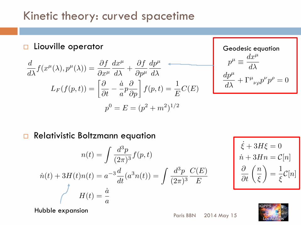
Kinetic theory: curved spacetime

¨  Liouville operator

¨  Relativistic Boltzmann equation


d

d�

f(xµ(�), pµ(�)) =@f

@x

µ

dx

µ

d�

+@f

@p

µ

dp

µ

d�

LF (f(p, t)) =

@

@t

� a

a

p

@

@p

�f(p, t) =

1

E

C(E)

p0 = E = (p2 +m2)1/2

Geodesic equation

p

µ ⌘ dx

µ

d�

dp

µ

d�

+ �µ⌫⇢p

⌫p

⇢ = 0

Hubble expansion

n(t) =

Zd3p

(2⇡)3f(p, t)

n(t) + 3H(t)n(t) = a�3 d

dt(a3n(t)) =

Zd3p

(2⇡)3C(E)

E

H(t) =a

a

⇠ + 3H⇠ = 0

n+ 3Hn = C[n]@

@t

✓n

⇠

◆=

1

⇠C[n]

Entropy production

¨  Boltzmann H-theorem ¤  Entropy current

¨  Equivalence relations ¤  Collision integral is zero; proper entropy is constant; equilibrium

distributions ¤  Collision integral non-zero; proper entropy generation; non-equilibrium


Sµ= �

Zd3p

(2⇡)3pµ

p0[f log f ⌥ (1± f) log(1± f)]

Sµ;µ = �

Zd3p

(2⇡)3log fC(E) � 0

Equilibrium =) Sµ;µ ⌘ 0

Equilibrium distributions

¨  Fermi-Dirac

¨  Bose-Einstein

¨  Maxwell-Boltzmann


ZBE =1X

N=0

⇣e��(✏�µ)

⌘N=

1

1� e��(✏�µ),

ZFD =1X

N=0

⇣e��(✏�µ)

⌘N= 1 + e��(✏�µ).

fFD = hNiFD =1

e�(✏�µ) + 1

fBE = hNiBE =1

e�(✏�µ) � 1

Cosmology notes 19

The average occupation of a quantum state with energy ✏ is

hNi =1

Z

X

N

X

s(N)

Ne��(✏s(N)�µN), (113)

=@

@(�µ)logZ . (114)

Taking the logarithmic derivative and defining fBE and fFD we obtain:

fBE = hNiBE =1

e�(✏�µ)� 1

, (115)

fFD = hNiFD =1

e�(✏�µ) + 1. (116)

Note that when the temperature is high, �(✏�µ) ⌧ 1, these distribution functions have thesame limit

fBE = fFD ⇡ e��(✏�µ) = fMB, (117)

corresponding to the classical, Maxwell-Boltzmann limit for distinguishable particles.It will be convenient later to have the number and energy density

n(T ) = g(T )

Z

d3p

(2⇡)3f(p), (118)

⇢(T ) = g(T )

Z

d3p

(2⇡)3pf(p), (119)

for relativistic (i.e., negligible mass) fermionic and bosonic species with µ = 0. For BE wehave:

nBE = gBE(T )⇣(3)

⇡2T 3, (120)

⇢BE = gBE(T )3⇣(4)

⇡2T 4. (121)

while for FD we have:

nFD =3

4nBE, (122)

⇢FD =7

8⇢BE. (123)

Here, we have defined the Riemann ⇣ function ⇣(s) =P1

n=1 n�s with values

⇣(3) ' 1.202, ⇣(4) =⇡4

90, (124)

and the FD(BE) state multiplicity functions gFD(gBE), which count the number of spin andinternal quantum numbers of the various species of particles. These are shown in Table II.

The indicated T dependence of the multiplicities is a recognition of the fact that thetemperature should be high enough to initate reactions with center of mass energies equal

The equilibrium distributions satisfy the condition that the collision integral is zero. But here we derive them from the grand canonical ensemble.

Kinetic regimes

!! Equilibrium !! Hubble exp. negligible for kinetics

!! Forward/Reverse rates detail balance !! Reaction rate sufficiently fast to explore

much phase space !! Caveat: FLRW no timelike Killing field

!! Kinetic !! Hubble exp. and reactions compete

!! Non-zero net=F-R rate !! Boltzmann H-theorem: dS/dt>0 but ~ 0

#! However, assume adiabatic

!! Decoupled !! e.g. Relativistic: T~a-1

!! Free-streaming; distribution frozen 2014 May 15 Paris BBN

d�34,12 = dn2h�34,12v12,reliReaction rate � � H(t)

� ' H(t)

� ⌧ H(t)

Cosmological transitions (Caveat Emptor)

0.0 0.5 1.0 1.5 2.0Têm0

2

4

6

8JHTêmL


50 3. Thermal History

Exercise.—Derive (3.1.45). Notice that this is nothing but the ideal gas law, PV = NkBT .

By comparing the relativistic (T � m) and non-relativistic (T ⌧ m) limits, we see that

the number density, energy density, and pressure of a particle species fall exponentially (are

“Boltzmann suppressed”) as the temperature drops below the mass of the particle. We interpret

this as the annihilation of particles and anti-particles. At higher energies these annihilations also

occur, but they are balanced by particle-antiparticle pair production. At low temperatures, the

thermal particle energies aren’t su�cient for pair production. Numerically, one finds that the

particle-antiparticle annihilation takes place mainly (about 80%) in the interval T = m ! 16m.

We see that this isn’t an instantaneous event, but takes several Hubble times.

Exercise.⇤—Restoring finite µ in the non-relativistic limit, show that

n� n = 2g

✓mT

2⇡

◆3/2

e�m/T sinh⇣ µ

T

⌘. (3.1.46)

QCD

EW

Figure 3.2: Evolution of relativistic degrees of freedom assuming the Standard Model particle content.

E↵ective Number of Degrees of Freedom

Imagine a system with a collection of di↵erent species, possibly in equilibrium at di↵erent tem-

peratures Ti. The total energy density ⇢tot is the sum over all contributions

⇢tot =X

i

gi2⇡2

T 4i J±(xi) , xi ⌘

mi

Ti. (3.1.47)

It is common to write this in terms of the ‘temperature of the universe’ T (typically chosen to

be the photon temperature T�),

⇢tot =⇡2

30g?(T )T

4 , (3.1.48)

⇢(T ) = g?(T )⇡

2

30T

4�

g? =X

i

gi

✓Ti

T�

◆4J⇡i(xi)

J�(0)

⇢(T ) =X

i=�,⌫j ,`±,...

Zd

3p

(2⇡)3f

i

(p)qp

2 +m

2i

=X

i

g

i

T

4i

2⇡2J

⇡i(xi

)

J

⇡i(xi

) =

Z 1

0d⇠ ⇠

2

p⇠

2 + x

2i

e

p⇠

2+x

2i + ⇡

i

, x

i

= m

i

/T

NB: Ti=T�

Ji(xi) ! ✓

⇣T � mi

6

⌘J(xi) ! arbitrary!

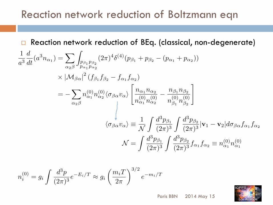
Reaction network reduction of Boltzmann eqn

¨  Reaction network reduction of BEq. (classical, non-degenerate)


h��↵v↵i ⌘1

N

Zd3p�1

(2⇡)3

Zd3p�2

(2⇡)3|v1 � v2|d��↵f↵1f↵2

N =

Zd3p�1

(2⇡)3

Zd3p�2

(2⇡)3f↵1f↵2 ⌘ n(0)

↵1n(0)↵1

n(0)i = gi

Zd3p

(2⇡)3e�Ei/T ⇡ gi

✓miT

2⇡

◆3/2

e�mi/T

1

a3d

dt(a3n↵1) =

X

↵2�

Z

p�1p�2p↵1p↵2

(2⇡)4�(4)(p�1 + p�2 � (p↵1 + p↵2))

⇥ |M�↵|2 (f�1f�2 � f↵1f↵2)

= �X

↵2�

n(0)↵1

n(0)↵2

h��↵v↵i"n↵1n↵2

n(0)↵1 n

(0)↵2

� n�1n�2

n(0)�1

n(0)�2

#

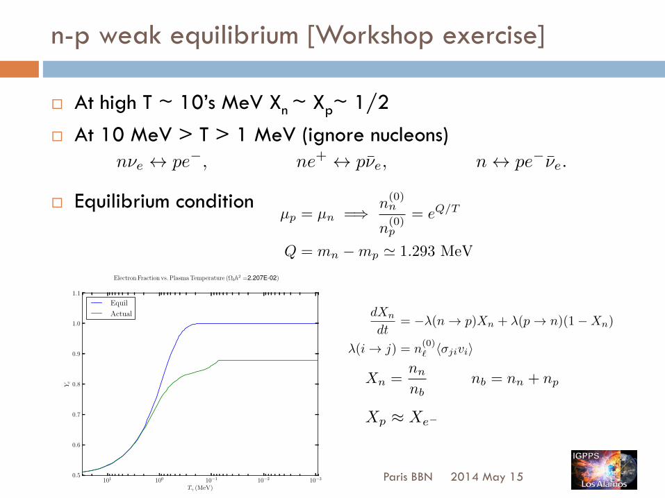
n-p weak equilibrium [Workshop exercise]

¨  At high T ~ 10’s MeV Xn ~ Xp~ 1/2 ¨  At 10 MeV > T > 1 MeV (ignore nucleons)

¨  Equilibrium condition


n⌫e $ pe�, ne+ $ p⌫e, n $ pe�⌫e.

dXn

dt= ��(n ! p)Xn + �(p ! n)(1�Xn)

�(i ! j) = n(0)` h�jivii

10�310�210�1100101

T� (MeV)

0.5

0.6

0.7

0.8

0.9

1.0

1.1

Ye

Equil

Actual

Electron Fraction vs. Plasma Temperature (⌦bh2 =2.207E-02)

Xn =nn

nbnb = nn + np

Xp ⇡ Xe�

µp = µn =) n(0)n

n(0)p

= eQ/T

Q = mn �mp ' 1.293 MeV

Big bang nucleosynthesis [Workshop exercise]

!! Full reaction network [NB: should be unitary]

!! Nuclear statistical equilibrium


10�210�1100101

T� (MeV)

10�24

10�22

10�20

10�18

10�16

10�14

10�12

10�10

10�8

10�6

10�4

10�2

100

Yi/

YH

N

D

T3He4He6Li7Li7Be

Relative abundances wrt YH vs. Plasma Temp. (⌦bh2 =2.207E-02)

1969ApJS...18..247W

dY↵1

dt=

X

↵2�

h� nbh��↵iY↵1Y↵2 + nbh�↵�iY�1Y�2

iYi =

ni

nb

End Lecture I


nuclear reactions in the early universe ihipacc.ucsc.edu/pdf/140729_2_paris.pdf · nuclear...

Documents