ntc thermistor performance and linearization of its
TRANSCRIPT

International Journal of
Advances in Scientific Research and Engineering (ijasre)
E-ISSN : 2454-8006
DOI: 10.31695/IJASRE.2020.33854
Volume 6, Issue 8
August - 2020
www.ijasre.net Page 35
Licensed Under Creative Commons Attribution CC BY-NC
NTC Thermistor Performance and Linearization of its Temperature-
Resistance Characteristics Using Electronic Circuit
K.T. Aminu, A. G. Jumba, A. A. Jimoh, A. Shehu, B. D. Halilu, S. A. Baraza,
A. S. Kabiru, and M. A. Sule
Department of Electrical Engineering
Abubakar Tatari Ali Polytechnic Bauchi
Nigeria
_______________________________________________________________________________________
ABSTRACT
This paper critically discusses the performance of an NTC thermistor sensor in the temperature range 20 oC to 85
oC
and provides a technique for linearization of the temperature sensed by the thermistor. The linearization was achieved
by utilizing Wheatstone bridge electronic circuitry which responds to the thermistor and produces an output which is
an exponential function of the temperature sensed by the thermistor sensor. A further simple and low-cost electronic
circuitry responds to such output and converts the resistance measurement to provide a signal which represents the
temperature. Moreover, the Wheatstone bridge signal conditioning circuitry was designed to have 0 – 100 mV output
voltage within the considered temperature range. The physical characteristics of the thermistor (constant A and b)
were found to be 4.0015 x 10⁻⁵
± 0.2956 x 10⁻⁵
Ω and 3514.8 ± 11.6 K respectively. The result also shows that the
percentage nonlinearity was as low as 1.7 and a sensitivity value of 1.5661 mV/K was found for the thermistor, but the
resolution of this thermistor sensor is 2 oC. However, the percentage of nonlinearity obtained was in agreement with
the theoretical percentage nonlinearity.
Keywords: Temperature measurement, Thermistor sensor, Practical design, linearization, Nonlinearity.
_______________________________________________________________________________________________
1. INTRODUCTION
In the recent decades, thermistor has been widely used for temperature measurement among a variety of applications.
Nevertheless, however, one of the most significant discussions in thermistor is that it is a piece of semiconductor made
from oxides of metal such as cobalt, iron, nickel, manganese, chromium and uranium pressed in into small wafer, disk,
bead or other shape fused at high temperatures and ultimately coated with glass or epoxy and produced in the form of
thick films, thin films and pellets [1] [2]. There are two types of thermistors namely: PTC (Positive Temperature
Coefficient) and NTC (Negative Temperature Coefficient). The PTC thermistor has its resistance increasing with
increasing temperature. Conversely, the NTC thermistor has its resistance decreasing with increasing temperature.
However, the NTC thermistors are the most commonly used type than the PTC thermistors, particularly for
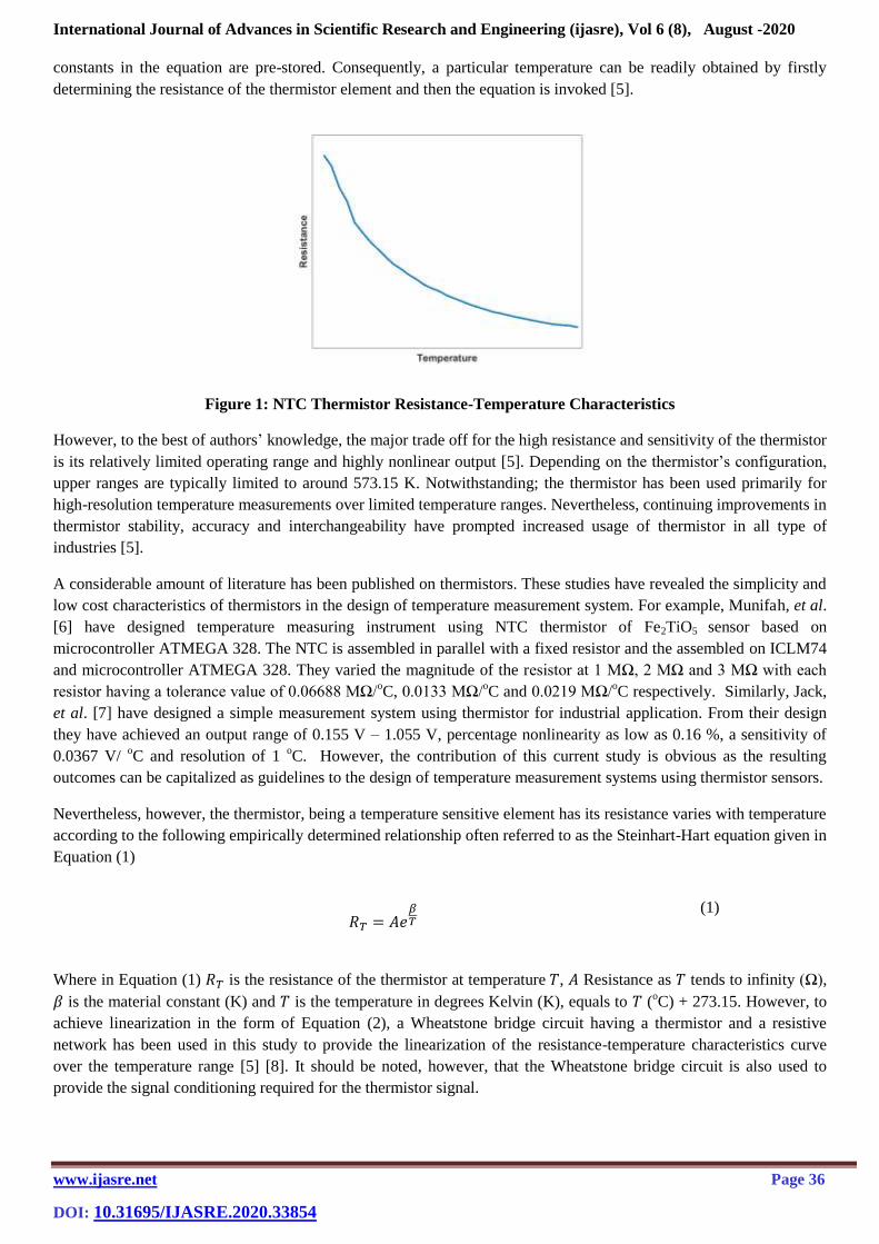
temperature applications [3] [4]. Figure 1 depicts the NTC thermistor Resistance-Temperature characteristics curve.
As far we know, thermistor sensors are very useful temperature measuring devices because of their high sensitivity,
high stability, repeatability, and large temperature coefficient of resistance so that variations in the thermistor’s
resistance provide a relatively high sensitive temperature sensing operation. On the other hand, one of the significant
problems in using thermistors, however, is that the relationship between the resistance and that of the temperature is a
non-linear one although such relationship can be expressed by a well known equation. Therefore, in order to make use
of thermistors over a wide range of temperature variations it is been found effective to pre-determine the resistance-
temperature relationship in accordance with such equation over a relatively wide range of temperatures and then the
International Journal of Advances in Scientific Research and Engineering (ijasre), Vol 6 (8), August -2020
www.ijasre.net Page 36
DOI: 10.31695/IJASRE.2020.33854
constants in the equation are pre-stored. Consequently, a particular temperature can be readily obtained by firstly
determining the resistance of the thermistor element and then the equation is invoked [5].
Figure 1: NTC Thermistor Resistance-Temperature Characteristics
However, to the best of authors’ knowledge, the major trade off for the high resistance and sensitivity of the thermistor
is its relatively limited operating range and highly nonlinear output [5]. Depending on the thermistor’s configuration,
upper ranges are typically limited to around 573.15 K. Notwithstanding; the thermistor has been used primarily for
high-resolution temperature measurements over limited temperature ranges. Nevertheless, continuing improvements in
thermistor stability, accuracy and interchangeability have prompted increased usage of thermistor in all type of
industries [5].
A considerable amount of literature has been published on thermistors. These studies have revealed the simplicity and
low cost characteristics of thermistors in the design of temperature measurement system. For example, Munifah, et al.
[6] have designed temperature measuring instrument using NTC thermistor of Fe2TiO5 sensor based on
microcontroller ATMEGA 328. The NTC is assembled in parallel with a fixed resistor and the assembled on ICLM74
and microcontroller ATMEGA 328. They varied the magnitude of the resistor at 1 MΩ, 2 MΩ and 3 MΩ with each
resistor having a tolerance value of 0.06688 MΩ/oC, 0.0133 MΩ/
oC and 0.0219 MΩ/
oC respectively. Similarly, Jack,
et al. [7] have designed a simple measurement system using thermistor for industrial application. From their design
they have achieved an output range of 0.155 V – 1.055 V, percentage nonlinearity as low as 0.16 %, a sensitivity of
0.0367 V/ oC and resolution of 1
oC. However, the contribution of this current study is obvious as the resulting
outcomes can be capitalized as guidelines to the design of temperature measurement systems using thermistor sensors.
Nevertheless, however, the thermistor, being a temperature sensitive element has its resistance varies with temperature
according to the following empirically determined relationship often referred to as the Steinhart-Hart equation given in
Equation (1)
(1)
Where in Equation (1) is the resistance of the thermistor at temperature , Resistance as tends to infinity (Ω),
is the material constant (K) and is the temperature in degrees Kelvin (K), equals to (oC) + 273.15. However, to
achieve linearization in the form of Equation (2), a Wheatstone bridge circuit having a thermistor and a resistive
network has been used in this study to provide the linearization of the resistance-temperature characteristics curve
over the temperature range [5] [8]. It should be noted, however, that the Wheatstone bridge circuit is also used to
provide the signal conditioning required for the thermistor signal.

International Journal of Advances in Scientific Research and Engineering (ijasre), Vol 6 (8), August -2020
www.ijasre.net Page 37
DOI: 10.31695/IJASRE.2020.33854
(2)
2. METHODOLOGY
2.1 Materials
Thermistor, thermometer (liquid in glass, -10 oC - 110
oC), soldering iron, magnetic stirrer, an electromagnetic hot
plate with an attached retort stand, beaker, digital multi-meter, test-tube, cotton wool, safety goggle, pros kit,
connecting wires, test-tube, heat gun, insulating sheath, water, ice, cello tape, an electronic circuit board (vero board),
lead sucker, single output Dc power supply (0 – 30 V, 30 A), Digital multimeters, plywood piece, standard resistors
(1 KΩ, 8.2 KΩ, 1.8 KΩ and 390 Ω).
2.2 Methods
An experimental investigation will be conducted to explore the relationship that exists between the thermistor’s
resistance and temperature. A snap shot of the thermistor sensor, location and the entire prototype measurement
system is shown in Figure 2. The thermistor was a disc thermistor with coating generally measuring 2.5 mm to 3.8
mm in diameter. The thermistor leads are connected to the test clip and the thermistor is immersed in the beaker to the
depth that will provide best test results usually obtained by trial and error procedure. While testing, be careful no to
immerse the test clip in the water because the added mass may disturb the beaker’s equilibrium temperature. In
addition extra care must be taken throughout the testing process to ensure the resistance measurements have the best
repeatability and lowest uncertainty possible. This effort will prevent the introduction of unwanted errors that would
distort the actual drift characteristics of the thermistor. Moreover, always ensure to place the eyes vertically at right to
the thermometer scale when taking readings, to avoid errors due to parallax. In order to determine the characteristics
of the NTC thermistor, special consideration is given to the room temperature, the temperature range in step variation
of 2 oC and the thermistor’s resistance. The thermistor is mounted with the thermometer on the retort stand clamped
together with the test tube and a cotton wool in between to prevent heat from escaping to the atmosphere.
Additionally, a plywood piece is used to cover the beaker top for the same previous purpose. The beaker of water
containing the stirrer is placed on the electromagnetic hot plate which is connected to a DC power supply source. In
this stage, the design make use of excel spreadsheet and active electronic circuit using Wheatstone bridge to
accomplish the task.
Figure 2: Temperature Measurement System Based on Thermistor
In the second part of the experimental investigation campaign, the design of signal conditioning circuit based on
Wheatstone bridge using a numerical method will be considered. This is the linearization method employed to
linearize the output voltage of the thermistor as a function of the input temperature. It necessary that before the circuit

International Journal of Advances in Scientific Research and Engineering (ijasre), Vol 6 (8), August -2020
www.ijasre.net Page 38
DOI: 10.31695/IJASRE.2020.33854
is implemented, the value of the standard resistors available in the laboratory is measured. Excel spreadsheet is
adopted for this computation. The measured and the computed results of the resistance values will be compared with
that of the numerical design model. Figure 3 depicts the bridge circuit used as signal conditioning circuit for the
thermistor.
3. EXPERIMENTAL SETUP AND PROCEDURE
A series of experimental trials were carried using the setup shown in Figure 2. The room temperature was read and
recorded. Similarly, the thermistor resistance at the ambient temperature was read and recorded. The thermistor was
soldered to two wires and then insulated using the insulating sheath and heat from the heat gun was applied to fasten
the insulating sheath to the thermistor wires. The two wires were then connected to the digital multi-meter. The
thermistor was then tied to the thermometer using the cello tape, and usually lags behind the thermometer because of
its high sensitivity to temperature. It was then put inside the test-tube which was clamped on the retort stand, and
immersed in a beaker containing water. The beaker was already half-filled water and placed on the magnetic stirrer hot
plate. The magnetic stirrer hot plate was switched on and heating process begins. At intervals of 2 oC, corresponding
values of resistance of the thermistor for a temperature range of 20 oC – 85
oC (temperature increasing) and
temperature range 85 oC - 20
oC (temperature decreasing) were recorded.
4. RESULTS AND DISCUSSION
4.1 Characterization of the Thermistor
The resistance of the thermistor at room was measured as R25 o
C = 5.12 KΩ. Subsequent readings for the thermistor
resistance for both temperature increasing and temperature decreasing were taken and either of the two was plotted to
give the thermistor resistance-temperature characteristic curve as shown in Figure 4. The discussion of the results
begins with an analysis in order to characterize the NTC thermistor. The characterization is performed to obtain the
thermistor constants and respectively.
Vs
R4
Ra
Rb
RT
V1
V2
Vo
I
Figure 3 Bridge Circuit used in
linearizing the thermistor
characteristics

International Journal of Advances in Scientific Research and Engineering (ijasre), Vol 6 (8), August -2020
www.ijasre.net Page 39
DOI: 10.31695/IJASRE.2020.33854
Figure 4: Thermistor Resistance-Temperature Curve (left) and Thermistor Resistance-Temperature Curve
with trend line
Figure 4 is very helpful in understanding the concept of linearization. As can be seen qualitatively in Figure 4,
Equation (1) set forth above approximately represents a decaying exponential curve. The trend line is inserted to
facilitate the computation of the sensitivity and the percentage nonlinearity using Equation (3) and Equation (4)
respectively.
(3)
(4)
From Equation (3), the sensitivity of the thermistor was found to be -0.0719 KΩ/K and the percentage nonlinearity
was found to be 30.45 % which further evidenced that exponential relationship that exists between the resistance and
the temperature of the thermistor, thus depicting a highly nonlinear relationship. It should be noted that within the
measuring system, the temperature of the system usually rises and fall and thus introducing the temperature hysteresis
effect. The hysteresis setting is the amount of narrowness and wideness of the temperature reading. Therefore, plotting
both the values of resistance with increasing temperature and decreasing temperature against the temperature depicts
the hysteresis effect of the thermistor. This effect is depicted in Figure 5.
International Journal of Advances in Scientific Research and Engineering (ijasre), Vol 6 (8), August -2020
www.ijasre.net Page 40
DOI: 10.31695/IJASRE.2020.33854
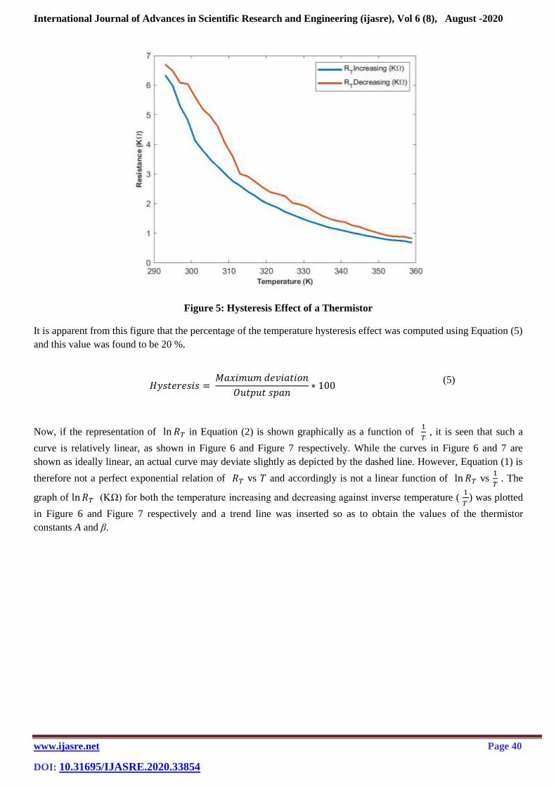
Figure 5: Hysteresis Effect of a Thermistor
It is apparent from this figure that the percentage of the temperature hysteresis effect was computed using Equation (5)
and this value was found to be 20 %.
(5)
Now, if the representation of in Equation (2) is shown graphically as a function of
, it is seen that such a
curve is relatively linear, as shown in Figure 6 and Figure 7 respectively. While the curves in Figure 6 and 7 are
shown as ideally linear, an actual curve may deviate slightly as depicted by the dashed line. However, Equation (1) is
therefore not a perfect exponential relation of vs and accordingly is not a linear function of vs
. The
graph of (KΩ) for both the temperature increasing and decreasing against inverse temperature (
) was plotted
in Figure 6 and Figure 7 respectively and a trend line was inserted so as to obtain the values of the thermistor
constants A and β.

International Journal of Advances in Scientific Research and Engineering (ijasre), Vol 6 (8), August -2020
www.ijasre.net Page 41
DOI: 10.31695/IJASRE.2020.33854
Figure 6: The graph of lnRtemp.increasing (KΩ) against 1/T (K-1
)
Figure 7: The graph of ln R temperature decreasing against 1/T (K-1
)
From Figure 4, to linearize the nonlinear relationship of the thermistor resistance with temperature, Equation (1) is
manipulated by taking the natural logarithm of the equation and the operation yields Equation (2). Recalling the
equation of a straight line (linear) graph i.e,
(6)

International Journal of Advances in Scientific Research and Engineering (ijasre), Vol 6 (8), August -2020
www.ijasre.net Page 42
DOI: 10.31695/IJASRE.2020.33854
Comparing Equation (2) and Equation (6) yields that, is linearly dependant on
. β is the slope of the straight
line and A represent the intercept. Also, by Equation (2) it is easy to see that the physical characteristics of the
thermistor (constants A and β) can be obtained.
From Figure 6,
The slope β = 3503.203 K
A = - 10.203, this implies that A = e-10.203
= 3.7059 x 10⁻⁵
Ω
Also From Figure 7,
The slope β = 3526.4 K
A = -10.055, which also implies that A = e-10.055
= 4.2970 x 10⁻⁵
Ω
The best result of β and A can be obtained by taking the average of the two quantities β and A (i.e taking uncertainty in
measurement into consideration)
βbest
= 3514.8 K
Abest
= 4.00145x Ω
It could be deduced that from Figure 4, the thermistor characteristics is nonlinear. It was also observed that the
thermistor’s resistance changes rapidly for every 2 oC temperature change; this has also confirm the assertion that
thermistor is very sensitive to temperature. The thermistor resistances were different for the same temperature values
when the temperature was increasing and when it was decreasing which indicates the hysteresis effect of the
thermistor (Figure 5). Figure 6 and Figure7 show that the linearization of the thermistor characteristics has led to the
determination of the best values for the thermistor constants (β and A).
4.2 Linearization Method
From Figure 4, 6 and 7, it has been found in accordance with this study that, by making some minor modifications, it
is possible to obtain a more perfect exponential relation of RT with T, or equivalently, a nearly perfect linear relation of
with T. These modifications may be performed by utilizing a Wheatstone bridge circuit shown in Figure 3
wherein a thermistor sensor having resistance RT connected in series with a resistor having resistance R4 has shunt a
resistor having resistance from the series combination of Ra and Rb in parallel therewith and a supply voltage in
series with the thermistor. The thermistor resistance for the various temperatures were computed using Equation
(1) where in the equation β = 3514.8 11.6 K and A = 4.00145x10⁻⁵ 0.2970 x 10
-5 Ω. The results obtained for
were recorded. Since the design was based on bridge circuit, then from Figure 3;
(7)
Where = output voltage of the thermistor, = supply voltage, which controls the output range (0 – 100 mV), =
resistance in series with the thermistor and is that control the linearization, = thermistor resistance at a given
temperature. Initially, for design purposes, the value of RT was taken to be 10 KΩ and the value as 0.21 V (210 mV)
and the corresponding values of at different temperatures were computed and plotted as shown in Figure 8

International Journal of Advances in Scientific Research and Engineering (ijasre), Vol 6 (8), August -2020
www.ijasre.net Page 43
DOI: 10.31695/IJASRE.2020.33854
Figure 8: The Graph of Thermistor Voltage V1 against Temperature
As it can be seen from Figure 8 the relationship is clearly nonlinear and to find the nonlinearity, a terminal line need
be defined and this line has a characteristics indicated by Equation (6). In Equation (6), Y = Vterminal voltage (V), M =
slope (V/K), X = input temperature (K) and C = intercept (V). The values of R4, VS, M and C were referenced
absolutely in the Exel spreadsheet workspace, such that a change in R4 or VS (during optimization) will affect the
whole computation process. However, for illustration purpose the values of M and C were computed from Figure 8. In
the computation process, the intervals (0.082618679 V, 293 K) and (0.014371416 V, 358 K) were considered.
M =
M = - 0.001049957 V/K
And C considering either of the interval
0.082618679 = - 0.001049957*293 + C
C = 0.39025608 V
The Vterminal was then computed using the above equation at different temperatures and the result was plotted as shown
in Figure 9.

International Journal of Advances in Scientific Research and Engineering (ijasre), Vol 6 (8), August -2020
www.ijasre.net Page 44
DOI: 10.31695/IJASRE.2020.33854
Figure 9: The graph of V1 and Vterminal vs Temperature
As Figure 9 shows, the relationship between V1 and Vterminal at different temperatures was seen; the design processes
involve optimizing the values of R4 within the standard values until the best linearity relationship is achieved. Since it
is R4 that determines the linearity, then VS determines the desired output range for the thermistor (i.e 0 – 100 mV). The
optimization for R4 and VS was done using the Excel spreadsheet (i.e manipulating R4 and VS and viewing until the
best linearity is achieved). The best linearity relationship was achieved at R4 =1.415 KΩ and VS = 0.21V (210 mV).
The percentage nonlinearity is computed using Equation (4). The corresponding values for V1, Vterminal at various
temperatures were computed and plotted as shown in Figure 10.
Figure 10: The graph of V1 and Vterminal vs Temperature
Similarly, the values of percentage nonlinearity computed using Equation (4) at various temperatures was plotted as
depicted in Figure 11.

International Journal of Advances in Scientific Research and Engineering (ijasre), Vol 6 (8), August -2020
www.ijasre.net Page 45
DOI: 10.31695/IJASRE.2020.33854
Figure 11: The graph of % Nonlinearity vs Temperature
The most striking result to emerge from this analysis is that, from Figure 11 the maximum percentage nonlinearity
was found to be 2 %. Practically, however, achieving the value of R4 = 1.415 KΩ was not successful, because of the
limitation placed on implementing its value (i.e only a combination of two standard resistors, either series or parallel
combination was allowed). Therefore, a near standard value of R4 = 1.39 KΩ (i.e 390 Ω and 1 KΩ in series) was
considered.
The new values for V1, Vterminal and % nonlinearity at the various temperatures were computed and plotted as shown
in Figure 12 and Figure 13 respectively.
Figure 12: The graph of V1 and Vterminal vs Temperature
International Journal of Advances in Scientific Research and Engineering (ijasre), Vol 6 (8), August -2020
www.ijasre.net Page 46
DOI: 10.31695/IJASRE.2020.33854
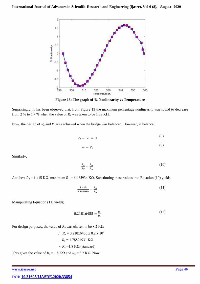
Figure 13: The graph of % Nonlinearity vs Temperature
Surprisingly, it has been observed that, from Figure 13 the maximum percentage nonlinearity was found to decrease
from 2 % to 1.7 % when the value of R4 was taken to be 1.39 KΩ.
Now, the design of Ra and Rb was achieved when the bridge was balanced. However, at balance;
(8)
(9)
Similarly,
(10)
And best R4 = 1.415 KΩ, maximum RT = 6.485934 KΩ. Substituting these values into Equation (10) yields;
(11)
Manipulating Equation (11) yields;
(12)
For design purposes, the value of Rb was chosen to be 8.2 KΩ
Ra = 0.21816455 x 8.2 x 103
Ra = 1.78894931 KΩ
Ra =1.8 KΩ (standard)
This gives the value of Ra = 1.8 KΩ and Rb = 8.2 KΩ. Now,

International Journal of Advances in Scientific Research and Engineering (ijasre), Vol 6 (8), August -2020
www.ijasre.net Page 47
DOI: 10.31695/IJASRE.2020.33854
(13)
(14)
(15)
The linearity relationship achieved at the value of R4 = 1.415 KΩ was depicted in Figure 10 and the maximum
percentage noninearity was found to be 2 % as seen in Figure 11. Because on the limitation placed on the practical
implementation of R4, a near standard value of R4 =1.39 KΩ was considered, and this changed the linearity
relationship to one seen in Figure 12 and the maximum % nonlinearity to 1.7 % as seen in Figure 11. The best value of
VS was achieved at VS = 0.21. Interestingly, however, increasing VS above this value has the effect of damaging the
thermistor, because more current will be flowing through the thermistor. This current will cause the self-heating of the
thermistor.
4.3 Implementation of the Design
The bridge circuit in Figure 3 realised from the design has Ra = 1.8 KΩ, Rb = 8.2 KΩ, R4 = 1.39 KΩ RT = variable
dependent on temperature, VS = 0.21 V. The temperature interval was increased from 2 oC that was previously used to
5 oC, this is to allow the thermistor to stabilize at the desired temperature before taking reading and this usually takes
longer time.
Repeated measurements were taken at temperature 323 K in order to obtain the best value Vo at that temperature.
Thus,
= 54.5 mV
The Standard uncertainty;
SN =
√ =
√ = 0.1238
Expanded uncertainty for 95% confidence;
= KU where U = 0.1238, K = 2.57 (from distribution table)
= 0.1238 x 2.57 = 0.3182
the best result for Vo at that temperature is 54.5 0.3182 mV
The performance test results were plotted as shown on Figure 14

International Journal of Advances in Scientific Research and Engineering (ijasre), Vol 6 (8), August -2020
www.ijasre.net Page 48
DOI: 10.31695/IJASRE.2020.33854
Figure 14: The graph of Vo against Temperature
This figure is quite revealing in some way. The output voltage response of the bridge circuit is relatively closely linear
over the temperature range. So long as the temperatures to be measured are confined to that range the output from the
thermistor circuitry using the resistance network is a linear function of the thermistor temperature. Additionally, such
circuitry will be relatively easy to calibrate.
5. CONCLUSION
This study set out to explore the performance of NTC thermistor and the linearization of its resistance-temperature
characteristics using electronic circuitry within the temperature range 20 oC - 85
oC. Interestingly, this study has
shown that using the temperature range 20 oC - 85
oC we were able to see the thermistor characteristics and determine
the best values of the thermistor constants (i.e β = 3514.8 11.6 K and A = 4.00145 0.2970 x 10⁻⁵
Ω). The
linearization of the thermistor output voltage was achieved by designing a signal conditioning circuit based on
Wheatstone bridge circuit whose output voltage was limited to the 0 – 100 mV. The designed circuit was
implemented; measurements were taken repeatedly at temperature 323 K to obtain the best value of the output voltage
for appreciation of uncertainty at that temperature. It was found to be 54.5 0.3182 mV. It was also shown that that
the percentage nonlinearity was as low as 1.7 and sensitivity value of 1.5661 mV/K was found for the thermistor, but
the resolution of this thermistor sensor is 2 oC. The percentage nonlinearity obtained is in agreement with the
percentage nonlinearity commonly obtained (theoretically) during the design of the circuit.
This research has thrown up many questions in need of further investigation. For example, considerable work will need to be done
to determine whether the use of high gain negative feedback and zero drift operational amplifier at the output of the thermistor’s
circuitry (bridge circuit) can improve the output voltage by removing loading effects and DC offsets. Moreover, research is
needed to implement the circuit design in such a way as to further reduce the self-heating effect of the thermistor.
REFERENCE
1. Wiendartun, R. and Fitrilawati, R. E. 2016. The Effect of Sintering Atmosphere on Electrical Characteristics
of Fe2TiO5 Pellet Ceramics sintered at 1200 oC for NTC thermistor, Journal of Physics: Conference Series
739
2. Zhang, D., Shi, M. J., Chen, L. L. and Ding, S. J. 2013. Designing of Thermistor Digital Thermometers based
on unbalanced Electric Bridge, Trans. Tech. Publications, Switzerland, Key Engineering Materials 538, Pp
133 – 137

International Journal of Advances in Scientific Research and Engineering (ijasre), Vol 6 (8), August -2020
www.ijasre.net Page 49
DOI: 10.31695/IJASRE.2020.33854
3. David, P. 1996. Measuring Temperature with Thermistors - a Turtorial, National Instruments Application
Note 065
4. Morris, A. S. 2001. Measurement and Instrumentation Principles, third edition
5. Newman, W.H., Mass, B., Burgess, R.G., and Hudson, N. H. 1992. Temperature Measurement Using
Thermistor Elements, Medical Physics, Vol. 10(3), Pp. 327 – 332
6. Munifah, S. S., Risdiana, W., and Aminudin, A. 2019. Design of Temperature Measuring Instrument Using
NTC Thermistor of Fe2TiO5 Based on Microcontroller, Journal of Physics: Conference Series 1280
7. Jack, K. E., Nwangwu, E. O., Etu, I. A., and Osuagwu, E. U. 2016. A Simple Thermistor Design for Industrial
Temperature Measurement, IOSR Journal of Electrical and Electronics Engineering, Vol. 11(5), Pp. 57 – 66
8. Chakravarty, R. K., Slater, K., and Fischer, C. W. 1977. Linearization of Thermistor Resistance-Temperature
Characteristics Using Active Circuitry, Review of Scientific Instruments, Vol. 48(12), Pp 1645-1649