n!st allldm msfist publigat!on|| nisr

NAT L INST. OF STAND & TECH R.I.C

AlllDM mSfiSTi|.

N!ST

PUBLIGAT!ON||

,?«i

Nisr United States Department of CommerceTechnology AdministrationNational Institute of Standards and Technology

NIST Technical Note 1364

Uncertainty Analysis of the

NIST Nitrogen Flow Facility

Jennifer L. Scott

Michael A. Lewis

Uncertainty Analysis of the NISTNitrogen Flow Facility

Jennifer L. Scott

Michael A. Lewis

Process Measurements Division

Chemical Science and Technology Laboratory

National Institute of Standards and Technology325 BroadwayBoulder, Colorado 80303-3328

Supersedes NBS TN 606

March 1994

U.S. DEPARTMENT OF COMMERCE, Ronald H. Brown, SecretaryTECHNOLOGY ADMINISTRATION, Mary L. Good, Under Secretary for TechnologyNATIONAL INSTITUTE OF STANDARDS AND TECHNOLOGY, AratI Prabhakar, Director

National Institute of Standards and Technology Technical NoteNatl. Inst. Stand. Technol., Tech. Note 1364, 48 pages (March 1994)

CODEN:NTNOEF

U.S. GOVERNMENT PRINTING OFFICEWASHINGTON: 1994

For sale by the Superintendent of Documents, U.S. Government Printing Office, Washington, DC 20402-9325

CONTENTS

1. Introduction 1

2. Uncertainty Evaluation 1

3. Liquid Nitrogen Flow Facility 4

3.1 Facility Description 4

3.2 Uncertainty in Liquid Nitrogen Mass Flow Measurement 6

3.2.1 Load Cell Sensitivity 6

3.2.1.1 Weights 7

3.2.1.2 Voltage 7

3.2.1.3 Sensitivity Equation 7

3.2.1.4 Pressure 8

3.2.2 Buoyancy Correction 8

3.2.2.1 Volume of Liquid in Weigh Tank 9

3.2.2.2 Density of Nitrogen-Helium Ullage 10

3.2.2.3 Volume of Diffuser and Pipe 11

3.2.2.4 Liquid Volume Accumulated before Measurement .... 11

3.2.3 Time 12

3.2.4 Volume between Test Section and Weigh Tank 12

3.3 Liquid Volume Flow Rate Measurement 13

4. Gaseous Nitrogen Flow Facility 14

4.1 Facility Description 14

4.2 Uncertainty in Gaseous Nitrogen Mass Flow Measurement 16

4.2.1 Weigh Tank Uncertainty 16

4.2.2 Gas Turbine Meter Uncertainty 17

4.2.2.1 Calibration Equation 18

4.2.2.2 Mass 18

4.2.2.3 Frequency 18

4.2.2.4 Density 19

4.3 Uncertainty in Orifice Meter Discharge Coefficient 20

5. Summary 25

6. Acknowledgements 26

7. References 26

ni

APPENDIX A.

APPENDIX B.

APPENDIX C.

APPENDIX D.

APPENDIX E.

APPENDIX F.

APPENDIX G.

LOAD CELL CALIBRATION WEIGHTS REPORTS ANDUNCERTAINTIES 27

NITROGEN PROPERTY UNCERTAINTY 31

UNCERTAINTIES IN ELECTRONICINSTRUMENTATION 32

UNCERTAINTIES OF QUARTZ BOURDON GAUGESUSED AS CALIBRATION PRESSURE STANDARD 34

UNCERTAINTIES IN PRESSURE SENSINGINSTRUMENTS 35

UNCERTAINTIES IN TEMPERATUREMEASUREMENT 40

UNCERTAINTIES IN DIMENSIONAL MEASUREMENTS . 44

IV

Uncertainty Analysis of the NIST Nitrogen Flow Facility

Jennifer L. Scott and Michael A. Lewis

National Institute of Standards and Technology

Chemical Science and Technology Laboratory

Boulder, Colorado 80303

An uncertainty analysis of the nitrogen flow facility at the National

Institute of Standards and Technology was performed. This facility functions

as a cryogenic flow calibration laboratory and as an applied research

laboratory for high pressure nitrogen gas flow measurement. This report

includes the analysis of uncertainty in liquid nitrogen mass flow, gaseous

nitrogen mass flow determined by a system turbine meter, instrumentation,

and the uncertainty in orifice meter discharge coefficient calculation using a

defined propagation of uncertainties technique. Uncertainties determined by

statistical means are distinguished from those determined by other means.

Key words: buoyancy; density; discharge coefficient; mass; propagation of

uncertainties; orifice meter; sensitivity; statistics; turbine meter; Type Auncertainty, Type B uncertainty

1. Introduction

This report provides a detailed description of the uncertainty analysis of the nitrogen

flow facility at the National Institute of Standards and Technology (NIST) in Boulder,

Colorado. This facility is used in two distinct ways. We calibrate and/or test cryogenic

flowmeters using a mass and time dynamic weigh system. After a system modification, wecan conduct applied research on gas flowmeters using the same weigh system. We focus the

uncertainty analysis in two areas: (1) the uncertainty associated with the determination of

mass flow rate, and (2) the uncertainty in measuring orifice meter discharge coefficients in

nitrogen gas flow.

2. Uncertainty Evaluation

We use the guidelines in NIST Technical Note 1297 [1] to classify the types of

uncertainties in our facility and to determine their values. We distinguish the components

of uncertainty determined by statistical analysis of observed data, called Type A, from those

determined by a priori information (for example, manufacturers' imcertainties for electronic

equipment). Type B.

Nearly all samples used to estimate Type A uncertainties contain more than 30

points. Most Type B uncertainties are those associated with instrumentation and

thermophysical properties, of the working fluids (hquid and gaseous nitrogen) where the

number of degrees of freedom is considered infinite. Following the guideUne in Technical

Note 1297, we assume that uncertainties stated by manufacturers are based on a rectangular

distribution; that is, the performance of the instrument will fall within the manufacturers'

uncertainty 100 percent of the time. To estimate a standard uncertainty of an instrument,

we divide the manufacturer's uncertainty by the square root of 3.

The combination of all uncertainties, in quadrature, is multiplied by a coverage factor

of 2 in order to estimate an approximate 95 percent confidence interval for total system

uncertainty. All sample sizes were large enough that a coverage factor of 2 is sufficient to

estimate a 95 percent confidence interval.

The key to determining the uncertainty in our system centers on our ability to

determine the uncertainty in crucial measurements of temperature, pressure, frequency, and

mass. Certain electronic instruments are common to many of these measurements. Ouranalyses of the uncertainties in these instruments, as well as the uncertainties in density

computation and dimensional measurements, are included in the Appendices. TheAppendices also contain uncertainty analyses of pressure and temperature measurements.

The information in these Appendices lays the groundwork for determining uncertainties in

measurements involving combinations of these values.

A first-order Taylor series expansion, commonly called propagation of uncertainty,

is used to determine the uncertainties in a quantity (such as, discharge coefficient) that is

calculated when the variables in the calculation have associated uncertainties. Equations

(1) and (2) show the general form used in evaluating propagation of uncertainties,

y = / (J^p x^y-.jc^) , (1)

«'(y) = Ei=l 6x..

n-l

"'i^,) - 2E E ^^ u (X, X) ,(2)

where y represents a quantity that is calculated as a function of n other quantities, Xi,...Xn,

and Uc(y) is the combined standard uncertainty of the calculated quantity. The third term

in Equation (2) represents the covariance between variables.

To determine uncertainties in many components of the flow system we combine

factors as though their relationship was multiplicative; that is, we sum the squares of the

individual uncertainties. Whenever the functional relationship can be determined, we use

the propagation of uncertainty. We do not include covariances because in no case did wedetermine that the uncertainty of one factor was a function of the uncertainty in another

factor. The following list describes notations used in this report.

Notation:

Type A Uncertainty determined by statistical means

Type B Uncertainty determined by other means

n Sample size

k A coverage factor that is multiplied by the combined standard

uncertainty to achieve a 95 percent confidence interval estimate

for total uncertainty. This product is called the expandeduncertainty, and in this analysis, k equals 2.

quadrature (a^ + b^ + ....)^, root sum of the squares

u(Xj) Estimate of the standard uncertainty (la) of the variable Xj

residual standard Standard deviation of the mean of the difference between knowndeviation values and those predicted by a model; root mean squared error

standard error s//n, standard deviation of the mean divided by the square root of

of the mean the sample size

T Temperature, K

V Voltage, VI Current, Ap Density, kg/m^

CY The product of the orifice meter discharge coefficient and the

expansion factor. This product is referred to as the discharge

coefficient in this document.

m Mass, kg

t Time, s

Ap Differential pressure; pressure drop across an orifice plate, kPa

static pressure Thermodynamic or line pressure, Pa

D Internal pipe diameter, cm

d Orifice bore diameter, cm

Fa Coefficient of thermal expansion for stainless steel

/5 Beta ratio, ratio of the orifice bore to the pipe diameter (d/D)

test point This phrase describes one mass measurement by either the weightank or a turbine meter. It may include any or all of the following

additional measurements: elapsed time, pulses, temperatures, andpressures.

Y Expansion factor

3. Liquid Nitrogen Flow Facility

3.1 Facility Description

The cryogenic liquid nitrogen facility, built by the National Bureau of Standards

(NBS) and the Compressed Gas Association, was commissioned in 1968. A detailed

description of the early capabilities and design information is given in NBS Report 9749 [2].

A provisional accuracy statement, NBS Technical Note 606 [3], was published in 1971

regarding the Hquid nitrogen system. The present report describes slightly different

techniques to evaluate uncertainty but relies on some of the results included in [3]. In

addition, changes in instrumentation and data acquisition since the pubUcation of Technical

Note 606 require a new uncertainty evaluation. This section describes the hardware of the

hquid facihty and the measurements required for flowmeter caUbrations.

Figure 1 is a schematic of the liquid flow facility. Liquid nitrogen is the process fluid

which is circulated throughout the closed loop by a variable speed boost pump. The liquid

flows into a subcooler where thermal energy due to pumping and ambient heat leak is

removed. The temperature of the liquid nitrogen in the flow loop can be changed or

controlled by adjusting the liquid level and the vapor pressure in the subcooler tank. Someof the test fluid also can be diverted around the subcooler, if necessary.

The path of the hquid nitrogen flow is shown in Figure 1. After leaving the

centrifugal pump, the hquid nitrogen passes through the subcooler and/or bypass, through

a vacuum-jacketed loop to the test section, and into a diffuser which removes the vertical

component of velocity at the bottom of a 0.378 m^ (100 gal) aluminum weigh tank. Thehquid flows through a valve at the bottom of the weigh tank and into a stainless steel

pressure vessel with a 0.443 m^ (117 gal) usable capacity. When the temperatures and

pressure in the system have reached a steady state condition, the weigh tank valve is closed

and Hquid nitrogen accumulates in the weigh tank.

Once the liquid reaches a preset level in the weigh tank, a test point begins. A timer

is initiated and a computer begins storing digitized information about the system and any

flow measurement device installed. For example, if a flowmeter with a frequency output

is installed in the test section, a counter begins totalizing the meter pulses while the

computer records digitized outputs from pressure transducers and thermometers.

A second, preset liquid nitrogen level marks the end of the test point. Data acquisition

stops and information from the timer and counters is sent to the main computer. A load

cell is used to measure the mass of the liquid accumulated in the tank. The load cell output

is recorded at the beginning and end of the test point so the difference in voltage is a

measure of the accumulated mass. The load cell is calibrated by suspending NIST-calibrated weights on the load cell before flowmeters are tested.

Helium is used as an over-pressurant in the catch and weigh tanks to control the

system pressure. The system is always over-pressurized to prevent boiling in the liquid

nitrogen. The nitrogen is always subcooled by 10 to 15 K. Helium absorption in the liquid

nitrogen is expected not to exceed 0.5 mole percent according to data by DeVaney, Dalton,

and Meeks [4]. No test points are taken if evidence of bubbles is detected visually through

a sapphire window located near the meter being tested.

The continuous flow loop allows for the establishment of system temperature,

pressure, and flow rate with the capability to maintain steady conditions for substantial time

periods. Typical calibration parameters are:

Flow rate: 0.95 to 9.5 kg/s (2 to 20 Ib/s)

Pressure: 0.4 to 0.76 MPa (60 to 110 psia)

Temperature: 80 to 90 K (144 to 162 °R)

3.2 Uncertainty in Liquid Nitrogen Mass Flow Measurement

The heart of our flow measurement facility is the weigh tank system. When wecalibrate cryogenic mass flowmeters, the uncertainty in the calibration data is equal to the

uncertainty in our mass flow measurement. The uncertainty in a calibration of a cryogenic

volume flowmeter depends on our ability to measure mass flow and liquid test-section

density. When we calculate the uncertainty in the discharge coefficient of an orifice

flowmeter, the uncertainty in mass flow is an integral portion of the propagation of

uncertainties associated with this calculated quantity. Consequently, we have included a

detailed description of our calculation of uncertainty in mass measurement. Thecomponents of mass uncertainty include those from the load cell, the buoyancy corrections,

time measurement, and changing mass between the test section and the weigh tank. Percent

uncertainties are based on a 181.4 kg (400 lb) test draft.

3.2.1 Load Cell Sensitivity

The mass of the liquid is measured by a load cell. The load cell is calibrated by

applying a series of certified weights on the load cell and measuring the output. At every

calibration point we measure both the excitation voltage (E^^^) to, and the output voltage

(Eq^) from, the load cell before and after the weight is added. Also, we measure the

pressure of the ullage surrounding the load cell. The sensitivity of the load cell at that point

is calculated as a ratio of the change in weight to the difference in the voltage ratios before

and after the weight is added. Equation (3) illustrates this calculation:

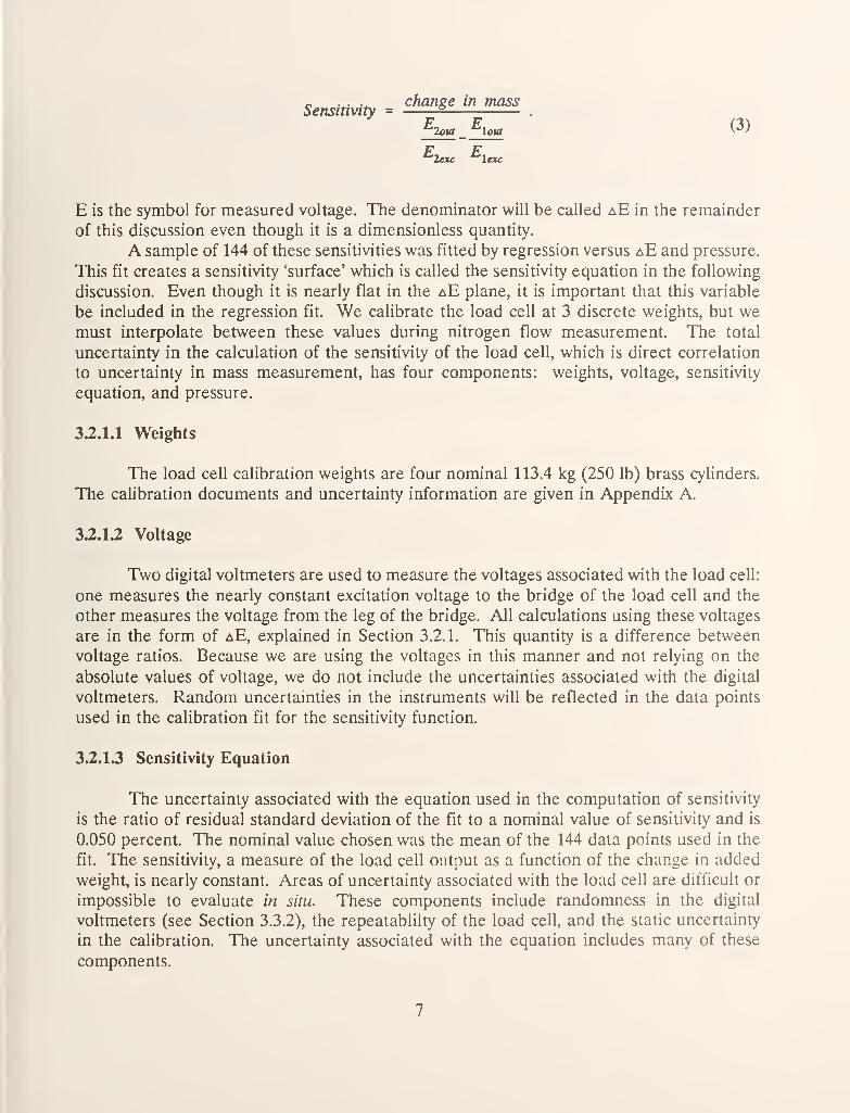
Sensitivity =<^'^"«" '" '^

^lout ^\out w)'lout _ lout

E is the symbol for measured voltage. The denominator will be called aE in the remainder

of this discussion even though it is a dimensionless quantity.

A sample of 144 of these sensitivities was fitted by regression versus aE and pressure.

This fit creates a sensitivity 'surface' which is called the sensitivity equation in the following

discussion. Even though it is nearly flat in the aE plane, it is important that this variable

be included in the regression fit. We calibrate the load cell at 3 discrete weights, but wemust interpolate between these values during nitrogen flow measurement. The total

uncertainty in the calculation of the sensitivity of the load cell, which is direct correlation

to uncertainty in mass measurement, has four components: weights, voltage, sensitivity

equation, and pressure.

3.2.1.1 Weights

The load cell calibration weights are four nominal 113.4 kg (250 lb) brass cylinders.

The calibration documents and uncertainty information are given in Appendix A.

3.2.1.2 Voltage

Two digital voltmeters are used to measure the voltages associated with the load cell:

one measures the nearly constant excitation voltage to the bridge of the load cell and the

other measures the voltage from the leg of the bridge. All calculations using these voltages

are in the form of aE, explained in Section 3.2.1. This quantity is a difference between

voltage ratios. Because we are using the voltages in this manner and not relying on the

absolute values of voltage, we do not include the uncertainties associated with the digital

voltmeters. Random uncertainties in the instruments will be reflected in the data points

used in the calibration fit for the sensitivity function.

3.2.1.3 Sensitivity Equation

The uncertainty associated with the equation used in the computation of sensitivity

is the ratio of residual standard deviation of the fit to a nominal value of sensitivity and is

0.050 percent. The nominal value chosen was the mean of the 144 data points used in the

fit. The sensitivity, a measure of the load cell output as a function of the change in added

weight, is nearly constant. Areas of uncertainty associated with the load cell are difficult or

impossible to evaluate in situ. These components include randomness in the digital

voltmeters (see Section 3.3.2), the repeatablilty of the load cell, and the static uncertainty

in the calibration. The uncertainty associated with the equation includes many of these

components.

The form of the sensitivity equation also accounts for dynamic uncertainties in the

load cell signal. During load cell calibration, we suspend three discrete weights from the

load cell. During a data point, the weight on the load cell is varying dynamically as the

weigh tank is being filled with liquid nitrogen. We do not evaluate the possible uncertainty

in the load cell due to these dynamic conditions. The only way to quantify these dynamic

uncertainties would be through a reference meter; however, the magnitude of the dynamic

uncertainty would be orders of magnitude smaller that the uncertainty associated with any

reference meter.

3^.1.4 Pressure

The uncertainty associated with the pressure measurement contributes to the

uncertainty in the sensitivity because it is an independent variable in the sensitivity equation.

The uncertainty evaluation for the ullage pressure transducer, P9, is included in AppendixE. Using the propagation of uncertainties technique shown in Section 2, we assessed the

additional uncertainty in sensitivity due to pressure at 10'^ percent, essentially zero. Table

1 lists the uncertainties associated with the load cell sensitivity.

Table 1. Load Cell Sensitivity Uncertainty (la)

Uncertainty in Sens. Type A TypeB

Equation 0.050%

Weights 0.002%

Total (in quadrature) 0.050% 0.002%

3.2.2 Buoyancy Correction

The buoyancy of the mass of liquid nitrogen collected in the weigh tank must be

evaluated for every mass measurement. There are three components to the correction in

mass measurement due to buoyancy: (1) the buoyancy of the Hquid nitrogen accumulated

during the data point, (2) the buoyancy of the immersed diffuser and pipe in the liquid, and

(3) the change in buoyancy of the liquid nitrogen accumulated before the data point begins.

The first two are reflected in the equation

B.C. = K,^ . p ullage- v_...

pipe 'liq(4)

where B.C. is the correction due to buoyancy, V,iq is the volume of the liquid nitrogen

accumulated during a data point, Punage is the density of the catch tank ullage, Vpip^ is the

volume of the diffuser and pipe immersed in the liquid nitrogen, and p^^ is the density of

the liquid nitrogen. The propagation of uncertainty for the buoyancy correction equation

follows:

(5)

uiV^f = mass

\ ^ui«(pflP (16)

tt(B.C.)^ = (p2 _

ullage

mass

'Uq

* "(P«,))' - (^fi, * ^(PuUa^:))'

^ ^-Vpipe * "(P/^)r

(7)

The first term on the right side of the equation represents the uncertainty in the buoyancy

due to hquid nitrogen density as it relates to Hquid nitrogen volume; the second, due to the

catch tank ullage density; and the third due to liquid density as it relates to the immersedpipe and diffuser. Each of these components will be addressed in the following sections, as

will the effect of the change in buoyancy of the liquid nitrogen accumulated before the data

point begins. The uncertainty calculations that follow represent the effect that these

uncertainties have on a nominal 181.4 kg mass.

322.1 Volume of Liquid in Weigh Tank

Our ability to determine the volume of the accumulated liquid nitrogen is a direct

result of our ability to evaluate the pressure, temperature, and, thereby, density of liquid

nitrogen. The uncertainty in the pressure (P9 and barometer) and temperature (T13)

measurement in the weigh tank are found in Appendices E and F. Appendix B outlines our

uncertainty evaluation for liquid nitrogen density. It includes the uncertainty in MIPROPS,the property software we use [5,6], as well as the uncertainty in density due to uncertainties

in temperature and pressure measurements. Using a 38-point data sample, we have

evaluated the effect of these density uncertainties on a nominal 181.4 kg mass. The results

are shown in Table 2.

Table 2. Uncertainties (la) in Mass Measurement Caused by Uncertainties in Liquid

Density

Source of Uncertainty in

Liquid Density

Percent change in a nominal 18L4 kg mass

Type A TypeB

MIPROPS 0.004%

6p/dT p (c7=0.5 K) 0.006%

6(>/dF T (P9,Baro) 0% 0%

Total (in quad) 0% 0.007%

3.2.2.2 Density of Nitrogen-Helium Ullage

The two most important factors in determining the density of the He-N2 mixture are

the temperature of the ullage in the volume surrounding weigh tank and the model used to

estimate the density of this mixture.

We use the Redlich-Kwong model, as modified by Chueh and Prausnitz, for the

binary equation-of-state calculation [7]. This model uses the catch tank ullage temperature

and pressure, and the liquid nitrogen temperature as input. When this model was adapted

to our system, empirical tests by NIST personnel led to an estimate of 3 to 5 percent

uncertainty in the ullage mixture density calculation using this model. Using a 38-point

sample of archival data, we determined the effect of the buoyancy correction on a 181.4 kg

mass measurement if the ullage density deviated by 4 percent. This value is shown in Table

3.

We also determined the sensitivity of this model to uncertainties in temperature and

pressure measurement. Three temperature measurements are involved in computing the

ullage density: the two ullage thermometers (TS71 and TS72) and the liquid nitrogen

thermometer (T13). The liquid nitrogen temperature is required to determine vapor

pressure. The uncertainties associated with these thermometers are shown in Appendk F,

and those for pressure are shown in Appendix E. These uncertainties in temperature and

pressure affect the ullage density calculation and, therefore, the mass measurement. Theresultant uncertainties on a 181.4 kg mass are shown in Table 3.

10

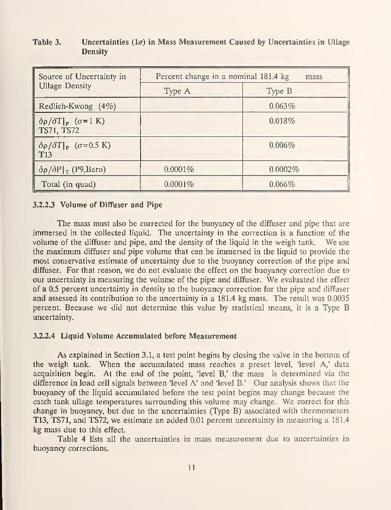
Table 3. Uncertainties (la) in Mass Measurement Caused by Uncertainties in Ullage

Density


Ullage Density

Percent change in a nominal 181.4 kg mass

Type A Type B

Redlich-Kwong (4%) 0.063%

dp/dT p (a=lK)TS71, TS72

0.018%

(5p/(5T p (a=0.5 K)T13

0.006%

6p/dF T (P9,Baro) 0.0001% 0.0002%

Total (in quad) 0.0001% 0.066%

3.2.2.3 Volume of Diffuser and Pipe

The mass must also be corrected for the buoyancy of the diffuser and pipe that are

immersed in the collected liquid. The uncertainty in the correction is a function of the

volume of the diffuser and pipe, and the density of the liquid in the weigh tank. We use

the maximum diffuser and pipe volume that can be immersed in the liquid to provide the

most conservative estimate of uncertainty due to the buoyancy correction of the pipe and

diffuser. For that reason, we do not evaluate the effect on the buoyancy correction due to

our uncertainty in measuring the volume of the pipe and diffuser. We evaluated the effect

of a 0.5 percent uncertainty in density to the buoyancy correction for the pipe and diffuser

and assessed its contribution to the uncertainty in a 181.4 kg mass. The result was 0.0035

percent. Because we did not determine this value by statistical means, it is a Type Buncertainty.

3.2.2.4 Liquid Volume Accumulated before Measurement

As explained in Section 3.1, a test point begins by closing the valve in the bottom of

the weigh tank. When the accumulated mass reaches a preset level, 'level A,' data

acquisition begin. At the end of the point, 'level B,' the mass is determined via the

difference in load cell signals between 'level A' and 'level B.' Our analysis shows that the

buoyancy of the liquid accumulated before the test point begins may change because the

catch tank ullage temperatures surrounding this volume may change. We correct for this

change in buoyancy, but due to the uncertainties (Type B) associated with thermometers

T13, TS71, and TS72, we estimate an added 0.01 percent uncertainty in measuring a 181.4

kg mass due to this effect.

Table 4 lists all the uncertainties in mass measurement due to uncertainties in

buoyancy corrections.

11

Table 4. Mass Uncertainties (la) Caused by Buoyancy Corrections

Mass Uncertainty due to

Buoyancy Corrections

Type A TypeB

Source: Liquid Density 0.012%

Source: Ullage Density 0.0001% 0.066%

Source: Diffuser/Pipe Vol 0.0035%

Source: Volume Before Point 0.01%


3.2.3 Time

In most cases, mass flow rate is used for meter calibration. A multi-function

datalogger is used to measure elapsed time. The uncertainty in time measurement is equal

to the resolution, 0.001 s. The contribution of time to the uncertainty in mass flow rate is

evaluated at a nominal time of 100 s. This is a Type B uncertainty.

Table 5. Uncertainty (lor) in Mass Flow Rate Caused by Time

Time Uncertainty TypeB

0.001 s @ 100 s 0.001%

32A Volume between Test Section and Weigh Tank

There is a finite volume of liquid nitrogen in the piping between the meter being

cahbrated and the weigh tank. A measure of the density gradient in the pipe is the

difference between fluid temperature at the meter end, Point A, and the weigh tank end of

the volume, Point B. We did not evaluate changes in density due to pressure drop because

there is no reason to believe that the pressure drop changes during a data point. If the

density gradient in this pipe remains constant during the data point, we assume that the

mass collected in the weigh tank is equivalent to the mass passing through the meter.

We evaluated changes in the density gradient in this volume for eight data points.

The average number of thermometer readings per data point was 165. We plotted the

difference between the temperature at the beginning of the pipe and the end of the pipe.

For thermally stable flows, this difference is constant and the slope through a regression fit

of these data is zero. A nonzero slope indicates that the density gradient and the mass in

the pipe are changing.

We found that the average change in the temperature difference between Points Aand B for the eight points evaluated was 0.067 K which translates to a 0.05 percent change

12

in liquid nitrogen density (Appendix B). The density of liquid nitrogen at nominal values

of 85 K and 586 kPa is 773.02 kg/m^. A 0.05 percent change in this density times a nominal

volume of the piping (0.05 m ) results in a 0.019 kg mass change in the piping. Theresultant uncertainty in a 181.4 kg mass measurement is 0.011 percent.

We did not include the uncertainties associated with the thermometers used in the

evaluation. They are included in other areas where the absolute values of the temperature

are needed. In this case, only the change in the difference between temperature

measurements was evaluated and not the differences themselves. The random variation of

the thermometers were accounted for in the regression fit of the temperature differences.

The following table exhibits all uncertainties associated with our measurement of

mass and mass-flow rate.

Table 6. Total Uncertainties (la) for Mass Measurement

Source of Uncertainty: Type A Type B Combined

Load Cell Sensitivity 0.050% 0.002% 0.050%

Buoyancy Correction 0.0001% 0.068% 0.068%

Mass between Test Section and

Weigh Tank (liquid Nj)

0.011%

Total for Mass Measurement 0.051% 0.068% 0.085%

Expanded Uncertainty, k=2 0.170%

Time 0.001% 0.001%

Total for Mass Flow Rate 0.051% 0.068% 0.085%


3.3 Liquid Volume Flow Rate Measurement

Our abiHty to accurately measure liquid nitrogen volume flow rate through the test

section depends not only on our ability to measure mass flow rate, but also on our

determination of liquid density. The transducers used to evaluate the pressure and

temperature of the Hquid in the test section are P7 and TIO. Their uncertainties are listed

in Appendices E and F. The uncertainties associated with density calculations are shownin Appendix B. Table 7 indicates the total uncertainty in determining liquid volume flow

rate. Density uncertainties were evaluated for liquid nitrogen at 85 K and 620 kPa.

13

Table 7. Uncertainty (1<7) in Volumetric Flow Rate Measurement


Liquid Volume Flow

Nominal Values: T = 85 K, P = 620 kPa,

Mass = 181.4 kg, Time = 100 seconds

Type A Type B

MIPROPS 0.25%

dp/dT\^ 0.025% 0.013%

6p/d? T (P7,Baro) 0.0002% 0.0002%

Uncert. in mass flow rate 0.051% 0.068%

Total (in quad) 0.057% 0.259%

Total (Type A+B, in quad), k=2 0.531%

Without MIPROPS uncertainty, k = 2 0.179%

The major contributor to the uncertainty of hquid nitrogen volumetric flow

measurement is the uncertainty in the liquid density. The greatest uncertainty in density

comes from the stated uncertainty in the equation of state (MIPROPS). When the objective

of using the uncertainty statement is in the mediation between seller and buyer, where both

have accepted the same values for density as determined by the NIST standard, the

uncertainty in density due to the equation of state need not be considered. In that case, the

expanded uncertainty in volumetric flow measurement for this laboratory (with k=2) is 0.18

percent.

4. Gaseous Nitrogen Flow Facility

The gaseous nitrogen flow loop has been used almost exclusively for applied orifice

meter research. Much of the following discussion centers around our determination of

uncertainty in orifice meter discharge coefficient.

4.1 Facility Description

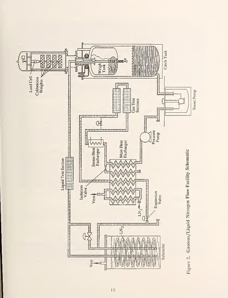
A schematic of the gaseous nitrogen flow facility is shown in Figure 2. All of the

components of the liquid system are used but, the flow is diverted as it leaves the circulating

boost pump into a fixed speed centrifugal pressure pump which increases the pressure of the

process fluid from 0,7 to 4.1 MPa (100 to 595 psia). We always operate at pressures above

3.5 MPa, the critical pressure of nitrogen; therefore, two-phase composition of the nitrogen

is avoided.

14

Thermal energy from three sources is added to the process fluid: (1) the ambient

surroundings, (2) a large counterflow plate-fin heat exchanger, and (3) a shell and tube heat

exchanger with steam on the tube side. The main heat exchanger is a five pass, plate-fin

type, constructed of aluminum and insulated with a 30 cm thickness of polyurethane foam.

The first pass in the main heat exchanger adds heat to the fluid through a counterflow

process with the returning fluid. Downstream of the first pass in the main heat exchanger,

a steam heat exchanger is used as a trim heater to control the temperature in the test

section. The typical test section temperature is 288 K. The process fluid returns through

the second pass of the heat exchanger, counterflow to the first pass, removing heat from the

return process stream. Two additional passages are used to exchange heat betweensubcooled liquid nitrogen and the returning process stream, removing additional thermal

energy from the process stream. One passageway is closed and used as a gas thermometer

(with pressure sensor) for heat exchanger monitoring and control purposes. If the pressure

in the gas thermometer remains constant during a test point, then the temperature is

constant and the rate of heat exchange is stable.

Process fluid flow is controlled by the operation of an expansion valve downstream

of the main heat exchanger, in conjunction with the variable speed circulating pump.Additional thermal energy is removed downstream of the expansion valve with the liquid

nitrogen bath subcooler mentioned in the liquid system description. At this point in the flow

loop, the process fluid is Hquid nitrogen and the load cell and reference described earlier

are used to complete the flow loop. To maintain stable operation of this system, a minimumflow rate of approximately 0.5 kg/s must be maintained and pressure drop in the gas loop

must be minimized (< 276 kPa, 40 psia).

This is a complex thermodynamic cycle, and even though it is highly instrumented,

it is difficult to quantify what is occurring at every element of the loop. The heat transfer

in the main heat exchanger is the most difficult to describe, but stability in the enclosed gas

thermometer reflects a stable heat exchange, that is, steady state flow, which is maintained

throughout the test point. If this stabiHty is maintained, the mass passing through a meter

in the gas portion of the loop is equivalent to the mass being collected in the weigh tank

during a data point. Because we can not quantify all uncertainties in this cycle, the gaseous

nitrogen flow loop is used only for applied research and not for calibrations.

4.2 Uncertainty in Gaseous Nitrogen Mass Flow Measurement

We measure mass flow in the gaseous nitrogen flow loop with either the weigh tank

described in Section 3.1 or by a gas turbine meter. The uncertainties associated with each

are discussed.

42.1 Weigh Tank Uncertainty

The uncertainties in measuring mass flow rate with the weigh tank are explained fully

in Section 3.2. The only difference between the analysis in Section 3.2 and the analysis

provided here is the possible change in mass in the piping volume between the test section

(gas versus liquid) and the weigh tank. If the system were totally stable, the mass in this

16

volume would remain constant during a data point.

As we explained in the description of the gas flow facility in Section 4.1, the nitrogen

in the piping between the gaseous nitrogen test section and the weigh tank is changed from

supercritical, ambient temperature nitrogen to liquid nitrogen. It is safe to assume that

during a 100 s test point, there may be some changes in density in subvolumes of this piping.

This would not be true for test points in which we measure nitrogen gas flow with the

turbines. The turbines are close to the orifice meter, and there is no phase change in the

nitrogen fluid between them.

We measure and record pressures and temperatures at many locations between the

test section and the weigh tank to quantify density changes in these subvolumes. Weanalyzed the changes in mass between the gas test section and the weigh tank as a function

of these density measurements recorded over a period of several years. We estimate that

the uncertainty (Type A) in a nominal mass of 181.4 kg due to the density variation in the

piping is 0.03%. Table 8 shows the uncertainties in gas measurement when using the weigh

tank.

Table 8. Total Uncertainties (la) for Mass Measurement in Gaseous Nitrogen Loop

Using Weigh Tank

Source of Uncertainty: Type A TypeB Combined

Load Cell Sensitivity 0.050% 0.002% 0.050%

Buoyancy Correction 0.0001% 0.068% 0.068%

Mass between Test Section and WeighTank (gas-liquid Nj)

0.030%

Total for Mass Measurement 0.058% 0.068% 0.089%


4.2.2 Gas Turbine Meter Uncertainty

The minimum flow rate at which the gaseous nitrogen flow loop can operate is

approximately 0.5 kg/s. We wanted to test orifice meters in the gas loop at lower flow rates,

so we added two gas turbine meters in series upstream of the orifice meter. We bypass part

of the flow before it enters the turbine-orifice meter loop so that total system flow is greater

that 0.5 kg/s. One of the turbines is used as the primary measurement device, while the

other serves as a constant reference to the primary turbine.

To determine the mass flow rate in the gas loop, the calibration curve for the primary

turbine is used to determine the volumetric flow rate during the test point. The density and

the mass flow rate are calculated using the temperature (T17) and the pressure (P17)

measured at the turbine meter. The uncertainty in the mass flow rate calculated from the

turbine meter is a combination of the uncertainties in the calibration equation, the counter

17

measuring turbine meter pulses, the mass flow rates used in the cahbration, and the density

at the turbine meter.

4.2.2.1 Calibration Equation

We calibrated the turbine meters over the range of our gas flow mass-based system:

0.5 to 2.3 kg/s (1.0 to 5.0 Ib/s). The turbine meters and associated piping were then sent

to an external facihty to be calibrated over a flow rate range of 0.11 to 1.1 kg/s (0.25 to 2.4

Ib/s). This calibration was done using air at pressures and temperatures similar to those at

which our facility operates. The calibration report included a stated flow measurementuncertainty of 0.5 percent.

The calibration data sets from NIST and the external laboratory were dissimilar and

difficult to resolve. The data set taken at the NIST laboratory contained 454 points and

showed more scatter than the 40 points from the external laboratory calibration. Weenlisted the help of the Statistical Engineering Division at NIST Boulder. They used a

nonlinear fitting to simultaneously calculate the parameters of a two-line fit for volume flow

rate versus frequency.

The calculation of uncertainty in the turbine meter calibration equation is not only

a function of the calibration curve fit, but the uncertainty in the mass flow reference system

of the facility performing the calibration and the density calculation. The turbine calibration

curve fit relies more heavily on the data from the NIST calibration, and the standard

uncertainty of the calibration is a reflection of the scatter from the NIST data. For these

reasons, we chose the uncertainties associated with measuring mass, time, and density at the

NIST lab to evaluate the uncertainty in the turbine meters.

The uncertainty in volumetric flow rate measured by the turbine meter due to the

calibration curve fit alone, at a nominal value of 1.81 kg/s, is 0.20 percent.

42.2.2 Mass

The uncertainty in mass measurement was provided in section 4.2.1. We use only the

Type B uncertainties here, because the Type A uncertainties are reflected in the calibration

data scatter and are included in the calibration equation uncertainty. Type B uncertainty

for mass measurement is 0.068 percent.

4.2.2.3 Frequency

The turbine frequency calculation is a combination of the output of the universal

counter and the timer in the datalogger. A manual trigger at the beginning and the end of

the measurement interval is used to signal measurements in both instruments. We totalize

the pulses from the turbine meter, and no test point has fewer than 2500 pulses. Because

the uncertainty in the counter is 1 pulse, the maximum uncertainty due to the counter is 0.04

percent. The Type B uncertainty in time measurement was shown in Section 3.2.3 to be

0.001 percent.

18

422.4 Density

The calculated fluid density at the turbine meter is used to determine the mass flow

rate in the gas flow loop. Table 9 lists the density uncertainties evaluated at the conditions

noted, along with the other contributors to turbine meter uncertainty. As in Section 3.7, the

expanded uncertainty is computed with and without the contribution of MIPROPS. Theuncertainty in our measurements due to MIPROPS would not be considered if all parties

were using the same property library.

Table 9. Uncertainty (la) in Mass Measurement Determined by the Turbine Meter

Source of Uncertainty

in Turbine Mass Flow

Nominal Values: T= 288.7 K, P=3.87 MPa,Mass = 181.4 kg, Time = 100 seconds

Type A Type B

Calibration Eq. 0.20%

Uncert. in mass 0.068%

Pulses 0.040%

Density: MIPROPS 0.10%

(5p/(5T p (T17) 0.029% 0.057%

dp/d? T(P17,Baro) 0.026% 0.070%

Total (in quad) 0.204% 0.156%

Expanded Uncertainty, I: = 2 0.513%

Without MIPROPS unceTtainty, k = 2 0.473%

The calculated uncertainty in mass measured by the turbine meter is more than twice

that of mass measured by the weigh tank because it contains the uncertainty of the weigh

tank as well as several other components (Section 4.2.2.1). When turbine-based mass flow

rates are used in the calculation of orifice meter discharge coefficients, this additional

uncertainty is not apparent. When we use both the turbine meter and the weigh tank to

measure the same mass flow rate, the orifice meter discharge coefficients calculated using

the turbine system calculated mass and those from the weigh tank system measured mass

are indistinguishable. The major contribution to the turbine meter uncertainty comes from

the curve fit to the calibration equation. The repeatability of turbine-based discharge

coefficients is 0.1 to 0.15 percent.

19

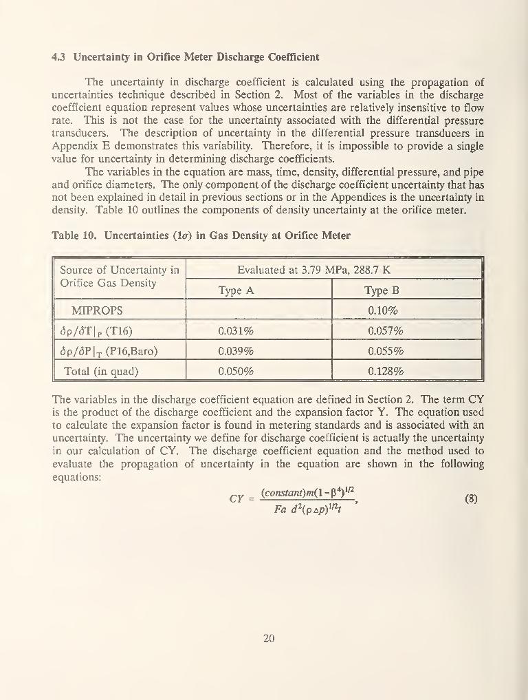
43 Uncertainty in Orifice Meter Discharge Coefficient

The uncertainty in discharge coefficient is calculated using the propagation of

uncertainties technique described in Section 2. Most of the variables in the discharge

coefficient equation represent values whose uncertainties are relatively insensitive to flow

rate. This is not the case for the uncertainty associated with the differential pressure

transducers. The description of uncertainty in the differential pressure transducers in

Appendix E demonstrates this variability. Therefore, it is impossible to provide a single

value for uncertainty in determining discharge coefficients.

The variables in the equation are mass, time, density, differential pressure, and pipe

and orifice diameters. The only component of the discharge coefficient uncertainty that has

not been explained in detail in previous sections or in the Appendices is the uncertainty in

density. Table 10 outlines the components of density uncertainty at the orifice meter.

Table 10. Uncertainties (la) in Gas Density at Orifice Meter


Orifice Gas Density

Evaluated at 3.79 MPa, 288.7 K

Type A TypeB

MIPROPS 0.10%

dp/6T p (T16) 0.031% 0.057%

dp/6? T (P16,Baro) 0.039% 0.055%

Total (in quad) 0.050% 0.128%

The variables in the discharge coefficient equation are defined in Section 2. The term CYis the product of the discharge coefficient and the expansion factor Y. The equation used

to calculate the expansion factor is found in metering standards and is associated with an

uncertainty. The uncertainty we define for discharge coefficient is actually the uncertainty

in our calculation of CY. The discharge coefficient equation and the method used to

evaluate the propagation of uncertainty in the equation are shown in the following

equations:

^Y = (constant)m(l-^*y'^ .g.

Fa d^pApy^t

20

where

5cr6</

tt(J)

\2

(bCY , y hCY6 Ap

ui^p)bCYbFa

u(Fa)]

(9)

bCY CYdm m

bCY CYbt t

dCY CYdp 2p

bCY _ CYb LP 2 LP

(10)

(11)

(12)

(13)

bCY _ -2cyp*^D (1-P*)d'

bCY 2CYbd d

bCY _ CYbFa Fa

'

(14)

(15)

(16)

u(Fa) = 1.51 X IQ-^uCI) .(17)

Therefore, uncertainties in the calculation of discharge coefficients are calculated by solving

the following equation with the appropriate uncertainties for all variables. We combined

the Type A and Type B uncertainties prior to this calculation:

21

^c(CY)Y _ (u(m)

CY mu(t)

\2

u(D)-2

d 1-p^+ 1

\2

\2-«(P)

2p J \ li^p )

' -uJAp)^ ^(" -LSljclQ-^uCT)

u{d)

\2

(18)

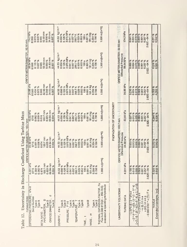
Tables 11 and 12 provide a detailed description of the components in the uncertainty

calculations of discharge coefficient for two differential transducers. Table 11 lists the

uncertainties when the weigh tank is used for mass measurement. Table 12 lists

uncertainties when the turbine is used for mass measurement.

22

c'4ii«

I

e

oU

t-i

C3X

03

t:

lOiJôoomono

_ o •*

I CO O) IQ Pi r«. « <o iSo c5 25rJ

E EE^ Eae

CO r«.eg

jRjRE EE# E#So to rÂ o> p

##E EEae Ese

S?

o o o >o o

CO h»o> o

E EaeaR E# E^

c2JS*P*^SPo)hr'Ooooi-otoo

*^ ## E# E^gin r- «o •* r^ to 51- 05 C?5 r>- «« Qi to

^- fS°- °. «- 8 P o>OJ*OOOi-0<00

##E E£3? E^

•- lO ^ CMCM * ts. lO 5 3- r«- -i w 00 o. -PSPqjPo o o ^ o to o

LU ._

^£ < CD

Lij z 8.8.QC T- >< >>a:.]5i-i-

T3

a CD QC CD

<$ •^

of

CD

Q

o

— OS

CO p 00 lO »- r«. r>» I

u5 SS CM r~

TtP'^*!*-!V66"'-!'~Hoo'•*OOeOOOCMOO 0''-00

r>» o> CO p •- »» op I

S'& 2 * 2 T-" S '

P P '-P CO P'

2-«E

f

2"«E,

«Op001OT-l>^t»-O)C0pi-'»fîs^SoSSgisiSs^ddcooocMod ~o »- o o 1-

09 lO T- fs. h- I

?J t^ ^ t"

«E.

ESpg9iOT-fs.h-g)«op»-T»-eDiS<^t;S!Qo6Sia*2'r-:S'*PT*PP3PP'~PfloP'^ o o CO o o e\j o o oôi

^S^^

2-«E,

E2pooini-Krô>e5P'-'«*-ooê5»-oo6ogbo^55o•*OOC0OOCMOO O '- O O y-

— (0

SpflOtn»-t«.r«.o>rtp»-'*floooÔ'-ooPogboT-SSdS'ÔOCOOOCMOO pT-OO

2«E,

E

O)..

-^ (0

flO!rtr-N.^-9>c5P'-'ôooo p

do d -- d d -r^

s•* O O CO O O CVJ I

< CO

c(D

a

CO

UJDC

mcra.

<CQH-<CD CD <CDq8.8.,-8.8. 8. 8.8.W

ID 2co' S.

I

Li. ®

UJ0.

v>

CJ)

§o. w

o-o+ 0)

.7 "S

Z

UJo

<OocQ.

EES5

Si

oc

o

OC TB

UJ 2S

cco

0)Q.

a

5EE

3

^ inUJ ig

^« "S « Q.^ O ÔQ-gOCTB-:'"1^J

&— O)

<rO

a

U. CO

UJ 2

zO

oUJ

<Q

SSod d d

jR jR jR

Solo d d

## jR

p « o>n w T-CM o oodd

K CO

Soodd

SR jR jR

o od d o

T- Od d o

< :

CD «

^ +

CMQ<

3 < Î ffl «

« -5CM ~>,

I csJ

jR jR jR aR

SSoI

d d d at

CM

aR jR jRaRo> -^ w ^

I

(O

c\j

d d d I

jR jR jRaR

SSO O O UJ

CMCO

ae# jR#Oi 1- O) 5

d d d UJ

CM

# jR SR jR

O O O UlCM

SR 3? JR jR

05 •- 0> 5-

8SS?d d d ui

CM(OCM

coD ®fÊ

(0

u.

OT I

f (0 3

o 3 =I

oI

•- CM

aR#

csj la

d d

o>-_ CO

d d

3«#[p CM

•- CMd d

CM •*

d d

i3

CM

c"a

9 "^

E E## E3R E#

|gj*rP*. CNJPs-PK»ao00ou)ono

(A

63

0)c3u

^ E ESfe ## Ej8 E#

SoPP*cJP2rP<-Sooou5ono

:5g

E EE# E#

P5 h-^ ^ 05 OS?l

,o o o m o I

## E EE# E#

•* h. lO iig^g:

01)

e

Dcs

ouex)

(A

i« E E1^ ## E# E#

|Cg<0oOOT-O<0d

—lO'-OOOpgppr-O^fil^-'ÔOCOOOCMOO ~

«E

o »- o o »-

2-«E

»£ jR aR 2 jR # 5*: jR # M jR S'jR jR ^

?-0'«-oooogoP'»-o5"!T Pd d CO d d CM d p O'r-oo '<-

E EE# E#

"'O00'-0<00

DC 9

"jR 5« 2 a? JR >^ JR JR w JR S'jR jR

« O 03 If^ T" f^ f~

'^ d d ro d d CM o o185258'-Poo*Hto T- p o

«E

f

-» cd

-*jRjR2jRjR:^jR#coJR ™JR JR

^ d d CO d d CM d d dt-do

"jR #2##^jR3RwjR 5'jR #

^ddcoddcMdd ~

2-«E

2"«E

1

p »- o p .-

i

ZULozo

ocrOl

^ (0

>t##2jRaR^jRjR wjR 5'jR jR

*ddcoddcMdd ~

2"«E

1

O »- OO 1-

E < en " CD arm

< ^ DC

m

c I

0)

T3

^'

o

<a)48.81'.>».>>c

;mt- < ffi CD

-25OC in To

LL , SZ Vy. 0><CDo^ =

88«wl^î5 8

tu

Z3

%LU

LUa.

Si

m ^

_ W^ a. <»

^ " -i

oScCM

S

a:

CC1B »;

p

aCCo

M^ ID i

nD.

s

V}zo

IoLU

a

<atu

ZCOcr

3r* oN J^

^ ^ o>

odd

jRjR jR•* o>

SoId d d

jR jR jR

CM O Oodd

jR jRjRK CO

35odd

aRsR jR

CO

oId d d

JRSR jR

S2<- oodd

# jRjR jR

lo> »- h". 5-Stn o

CMI

IP d d tu

|jR jR jR jR

8'" lO SCM

Io d d tu

CM

SR jR jR jR

o) •»- r«. ^^

S8«?d d d tu

CM

jR JR jRaRb> ••- 1*. i8 in o

CMI

Id d d LLi

IjRjR jR jR

S'"

in oCM

I

|d d d 111

CM

jR jR# JR

lo> 1- 1^ S8in pCM

Id d d LU

CM

< :

CQ «

f^ 1 â. CCM

^ +

Q<~~ CC

I CD

* «1CM -«

I CMI

N I

d o

aRjR

CM 5$d d

c ^^ ® «EP c «?j E a 3

3 9I

dI

Id dg

#V5

P P

aR:^CM I

h.CMId d

d p

CMIt

31

O 3•D

iS

24

5. Summary

Table 13 lists what we consider to be important overall uncertainties associated with

this laboratory. These values are an estimate of a 95 percent confidence interval using a

coverage factor of 2. Once again, values both with and without the contribution of the

density uncertainty due to MIPROPS are given.

Table 13. Uncertainty (la) Summary

Flow Measurement Uncertainty Evaluated for 181.4 kg mass, 100 s (k = 2)

Device: Weigh tank With MIPROPS Without MIPROPS

LNj "^^s flow 0.170% 0.170%

LNj volume flow 0.530% 0.178%

N2 gas mass flow 0.179% 0.179%

Device: Turbine

Gas N2 mass flow 0.513% 0.473%

The uncertainty in discharge coefficient calculation, a component of which is mass

flow rate, is variable and is better illustrated by plotting the relationship between uncertainty

and pressure differential for the transducers described in this report. Figure 3 demonstrates

this more complex uncertainty evaluation (MIPROPS uncertainty included).

1.50

+->

CCO

u<v

o

DaU

1.25 -

1.00 -

0.75 -

0.50

0.25

0.00

-0.25

-0.50

-0.75

-1.00

-1.25

-1.50

Trans 6715-weigh tank-Trans 6715-turbineTrans 8 1000- weigh tank-•Trans 81000-turbme

_L

40 80 120 160

Differential Pressure, kPa

1.50

1-25

1.00

0.75

- 0.50

H 0.25

0.00

^ -0.25

-0.75

-1 00

-1.25

-1.50200

Figure 3. Discharge Coefficient Uncertainty vs. Differential Pressure

25

6. Acknowledgements

We acknowledge the assistance of Mary Yannutz in document preparation, JimBrennan for technical support, and Jolene Splett from the NIST Statistical Engineering

Division for statistical expertise.

7. References

[1] Taylor, B.N.; and Kuyatt, C.E,, Guidelines for evaluating and expressing the

uncertainty of NIST measurement results, Natl. Inst. Stand, Technol. Tech. Note

1297, 1993.

[2] Mann, D.B.; Dean, J.W.; Brennan, J.A.; and Kneebone, C.H., Cryogenic flow

research facility, Natl. Bur. Stand. (U.S.) Report 9749, 1970.

[3] Dean, J.W.; Brennan, J.A.; Mann, D.B.; and Kneebone, C.H., Cryogenic flow

research facility provisional accuracy statement, Natl. Bur. Stand. (U.S.) Tech. Note

606, 1971.

[4] DeVaney, W.D.; Dalton, B.J.; and Meeks, J.C. Jr., Vapor-liquid equilibria of the

helium-nitrogen system, J. Chem. Eng., Data, 8, No. 4, 1963 October.

[5] NIST Pure fluids database [MIPROPS], Natl. Inst. Stand. Technol. 1986.

[6] Younglove, B.A., Thermophysical properties of fluids. I. Argon, ethylene,

parahydrogen, nitrogen, nitrogen triflouride, and oxygen, J. Phy. Chem. Ref. Data,

11, 1982.

[7] Chueh, P.L; and Prausnitz, J.M., Vapor-liquid equilibria at high pressures:

Calculation of partial molar volumes in non-polar liquid mixtures, AIChE J., 13,

1099-1107, 1967.

26

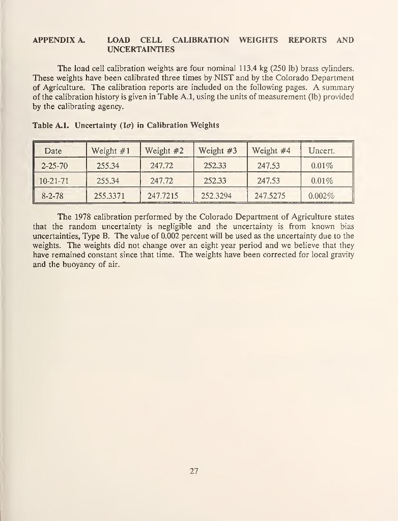
APPENDIX A. LOAD CELL CALIBRATION WEIGHTS REPORTS ANDUNCERTAINTIES

The load cell calibration weights are four nominal 113.4 kg (250 lb) brass cylinders.

These weights have been calibrated three times by NIST and by the Colorado Department

of Agriculture. The calibration reports are included on the following pages. A summaryof the calibration history is given in Table A.l, using the units of measurement (lb) provided

by the calibrating agency.

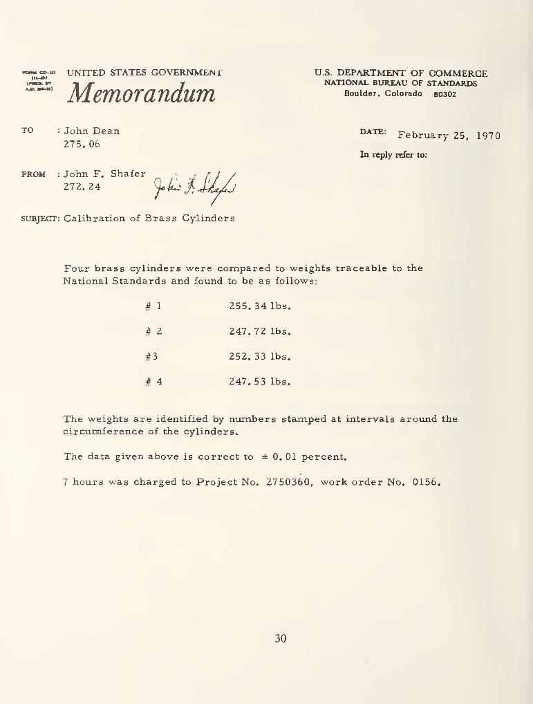
Table A,l. Uncertainty (la) in Calibration Weights

Date Weight #1 Weight #2 Weight #3 Weight #4 Uncert.

2-25-70 255.34 247.72 252.33 247.53 0.01%

10-21-71 255.34 247.72 252.33 247.53 0.01%

8-2-78 255.3371 247.7215 252.3294 247.5275 0.002%

The 1978 calibration performed by the Colorado Department of Agriculture states

that the random uncertainty is negligible and the uncertainty is from known bias

uncertainties, Type B. The value of 0.002 percent will be used as the uncertainty due to the

weights. The weights did not change over an eight year period and we believe that they

have remained constant since that time. The weights have been corrected for local gravity

and the buoyancy of air.

27

Richard D. Lamm

Governor

J. Evan GouldingCommissioner

Donald L. Svedman

Deputy Commissioner

sgv^ a^l>Q.

COLORADO DEPARTMENT OF AGRICULTURE406 STATE SERVICES BUILDING

1525 SHERMAN STREETDENVER, COLORADO 80203

August 2, 1978

REPORT OF TEST

for

Four special purpose test weights

OWNER: National Bureau of Standards, Cryogenic LaboratoryBoulder, Colorado

SUBMITTED BY: J A Brennan

AGRICULTURAL COMMISSION

Clarence Stone, CenterChairman

William A. Stephens, GvpsumVice-C hairman

Ben Eastman, HotchkissJohn L. Mailov, DenverM. C. McCormick, Holly

Elton Miller. Fort Lupton

Kay D. Morison. Fleming

William H. Webster, Greeley

Kenneth G. Wilmore, Denver

Cert. No: ^k^^

The test weights described above have been compared with the Standards of the Stateof Colorado and the following results have been determined:

Weight #1#2

#3

255.3371 lbs

247.7215252.32942.^7.5275

Uncertainty 0.0052 lb.

The uncertainty figure is an expression of the overall uncertainty using threestandard deviations as a limit to the effect of random errors of measurement, themagnitude of systematic errors from known sources being negligible.

F H Brzot).cky , j;!!'hief MetrologistColorad6 Depaij^ment of AgricultureMetrology Laboratory3125 Wyandot St.

Denver, Colorado 80211

THESE CERTIFlCATiCNS ARE TRACEABLE TO THE

fJATSONAL BUREAU CF STAIJDARDS.

ALL CERTIFICATES ISSUED BY THE COLORADO

^W'^T^-NT OF AGRiCULTURZ-METROLOGY LAB-

C.RhTGRY "expire one YEAR FROM THE DATE BF

ISSUANCE.

28

Date: October 12, 1971

X'ot: John Shafer, 272.55

Subject: Calibration of Brass Cylinders

To: Jim Brennan, 275*06

U.S. DEPARTMENT OF COMMERCEIMational Bureau of StandardsBouldar. Colorado 80302

Four brass cylinders were compared to weights traceable to the NationalStandards and were foimd to be as follows

:

#1 255.3^ lbs.

#2 2U7.72 lbs.

#3 252.33 lbs.

i^ 2i^7.53 lbs.

The weights are identified by numbers stamped at intervals around thecircumference of the cylinders

.

The measurements were made March k, 1971*

The data given above is correct to ±0.01 percent.

Six hours were charged to 2750161

.

29

»<cD-ui UNITED STATES GOVERNMEMl(ii-a)

"" MemorandumU.S. DEPARTMENT OF COMMERCENATIONAL BUREAU OF STANDARDS

Boulder, Colorado 80302

TO : John Dean275. 06

FROM : John F. Shafer

272. 24 Q*^J

SUBJECT: Calibration of Brass Cylinders

DATE: February 25, 1970

In reply refer to:

Four brass cylinders were compared to weights traceable to the

National Standards and found to be as follows:

# 1

# 2

#3

# 4

255. 34 lbs.

247.72 lbs.

252. 33 lbs.

247. 53 lbs.

The weights are identified by numbers stamped at intervals arotind the

circunnierence of the cylinders.

The data given above is correct to ± 0. 01 percent,

7 hours was charged to Project No. 2750360, work order No. 0156.

30

APPENDIX B. NITROGEN PROPERTY UNCERTAINTY

Depending on the location in the flow system, we are measuring subcooled liquid

nitrogen or gaseous nitrogen (supercritical) flow. The properties of these fluids are

calculated using a computerized package, NIST Pure Fluids Database (MIPROPS) [5]. Thenitrogen property information in the database was taken from a report by B. A. Younglove

[6]. The uncertainty expressed by Younglove for the density values of nitrogen were Txr,

therefore, the uncertainties that we list in our table are the stated uncertainties divided by

2. The density uncertainties are different for the two phases of nitrogen that are in our

system. Table B.l lists the uncertainties in the density. We also include the change in

density associated with small changes in temperature and pressure. These values are used

to evaluate density uncertainties in various regions of the flow system using the Type A and

Type B uncertainties associated with temperature and pressure measurements.

Table B.l. Uncertainties (Itr) in Nitrogen Properties

Property Uncertainties Liquid Nitrogen

T=85K,P = 621kPaGaseous Nitrogen

T=288.7 K, P=3.87 MPa

MIPROPSDensity 0.25% 0.10%

(5p/dT p 0.703% per K 0.378% per K

(5p/(5P|t 0.0005% per kPa 0.025% per kPa

31

APPENDIX C. UNCERTAINTIES IN ELECTRONIC INSTRUMENTATION

Most of the uncertainties described in this Appendix are those stated by the

manufacturers of the instruments. As outlined in Technical Note 1297 [1], we have assumedthat the stated manufacturers' uncertainties are based on a rectangular distribution which

has a standard uncertainty equal to the half-width of the specified interval divided by the

square root of 3. A description of the instruments follows, and Table C.l is a composite of

the Type B uncertainties that are incorporated into other calculations.

Multi-function Datalogger

The datalogger is used for several purposes. It measures the output of the constant-

current source, it supplies current to, and measures the voltage output from, two

thermometers located in the liquid catch tank ullage, and it measures elapsed time during

a test point.

Computer Analog to Digital Converter

The computer analog to digital (A/D) converter reads voltage outputs from as manyas 80 analog transmitters. Almost every transmitter in both the liquid and gas phase of the

flow loop is connected to this I/O device. All channels can be read at an approximate rate

of 100 times per second. Because of the resolution of this instrument, it provides the

greatest contribution to uncertainty of any electronic instrument.

Universal Counter

The universal counter counts the total number of pulses from any pulse-type meter

(turbine) in the gas flow system.

32

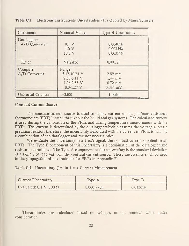
Table C.l. Electronic Instruments Uncertainties (la) Quoted by Manufacturers

Instrument Nominal Value Type B Uncertainty

Datalogger:

A/D Converter

Timer

0.1 V1.0 V10.0 V

Variable

0.0040%

0.0035%

0.0035%

0.001 s

ComputerA/D Converter^

Range:

5.12-10.24 V2.56-5.11 V1.28-2.55 V0.0-1.27 V

2.89 mV1.44 mV0.72 mV0.036 mV

Universal Counter >2500 1 pulse

Constant-Current Source

The constant-current source is used to supply current to the platinum resistance

thermometers (PRT) located throughout the liquid and gas systems. The calculated current

is used during the calibration of the PRTs and during temperature measurement with the

PRTs. The current is determined by the datalogger which measures the voltage across a

precision resistor; therefore, the uncertainty associated with the current to PRTs is actually

a combination of the datalogger and resistor uncertainties.

We evaluate the uncertainty in a 1 mA signal, the nominal current supplied to all

PRTs. The Type B component of this uncertainty is a combination of the datalogger and

resistor uncertainties. The Type A component of this uncertainty is the standard deviation

of a sample of readings from the constant current source. These uncertainties will be used

in the propagation of uncertainties for PRTs in Appendix F.

Table C.2. Uncertainty (la) in 1 mA Current Measurement

Current Uncertainty Type A Type B

Evaluated: 0.1 V, 100 Q 0.000 97% 0.0126%

^Uncertainties are calculated based on voltages at the nominal value under

consideration.

33

APPENDIX D. UNCERTAINTIES OF QUARTZ BOURDON GAUGES USED ASCALIBRATION PRESSURE STANDARD

Quartz Bourdon gauges are highly accurate pressure standards used to cahbrate

differential and static pressure transducers. The differential pressure transducers measure

the pressure drop across an orifice plate, and static pressure transducers measure line

pressure. The interlaboratory device we use to calibrate the Bourdon gauges is a dead-

weight tester calibrated by NIST. These calibrations have shown the Bourdon gauges to be

extremely stable over time. The resultant uncertainties from these calibrations are smaller

than those stated by the manufacturer, but, for simplicity, we have decided to take a moreconservative route and use the uncertainties supplied by the manufacturer. The contribution

of the uncertainty in these instruments to overall uncertainty in pressure measurement is

minimal.

The manufacturers' uncertainties for these instruments are defined as a percentage

of the range of the instrument and the reading at a specific pressure. The output of the

instrument, read by the datalogger, is a voltage which is proportional to pressure. Asoutlined in Technical Note 1297 [1], we have assumed that the stated manufacturers'

uncertainties are based on a rectangular distribution which has a standard uncertainty equal

to the half-width of the specified interval divided by the square root of three. The Type Buncertainties (Icr) for these instruments are:

0.0017% Range0.0030% Reading

The contribution of the uncertainties of these instruments to the uncertainty in pressure

measurements are calculated based on nominal pressures under consideration. These

nominal pressures are shown in the tables associated with each transducer found in

Appenduc E.

34

APPENDIX E. UNCERTAINTIES IN PRESSURE SENSING INSTRUMENTS

The uncertainty in pressure measurement has many components. They include the

standard error of the estimate of the caHbration equation, uncertainties in the calibration

standard (Appendix D), uncertainties in all electronic equipment (Appendbc C), as well as

dynamic variability observed during data points. The output from the static and differential

pressure transducers are digitized by the computer A/D converter. The data acquisition

channels and cables for the transducers are the same during calibration and actual operating

conditions. The signal from the quartz Bourdon gauge is read by the datalogger.

The dynamics of pipe flow create variabilities in the signals from the pressure

transducers that are not present during calibrations. We evaluated the dynamic variability

of the transducers by analyzing a sample of mean output values for the both the static and

differential transducers. Each value in the sample represents the mean of the readings

taken during a measurement (50 to 400 readings), and we analyzed at least 57 values for

each transducer.

Because static or line pressures vary little from data point to data point, the standard

errors of the means (s/Vn) for the sample of static pressure values were averaged. Theaverage was used as the dynamic uncertainty. We divided the dynamic uncertainty by a

nominal pressure for each transducer to determine the fractional uncertainty in pressure

measurement as a result of flow dynamics.

A slightly different approach was used to evaluate the dynamic variabilities in the

differential pressure transducers. The standard error of the means of the differential

pressure measurements were fitted versus the mean differential pressures. Using this fit, wedetermined the dynamic uncertainty at specific differential pressures shown in Tables E.6

and E.7.

Atmospheric and Static Pressure

The barometer which measures ambient air pressure is also calibrated with the quartz

Bourdon-tube gauge. The barometer reading is used for calibrating the static pressure

transducers and its uncertainty contributes to the uncertainty in the static pressure

measurement. The pressure range measured by static pressure transducers varies from 3.72

to 4.0 MPa (540 to 580 psia). The uncertainty for these transducers will be evaluated at a

nominal pressure of 3.87 MPa (562 psia). The following tables outline the uncertainties

associated with the static pressure transducers.

35

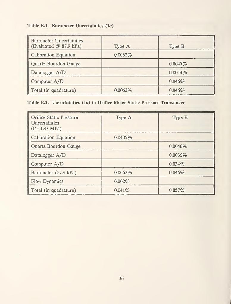
Table E.l. Barometer Uncertainties (la)

Barometer Uncertainties

(Evaluated @ 87.9 kPa) Type A Type B

Calibration Equation 0.0062%

Quartz Bourdon Gauge 0.0047%

Datalogger A/D 0.0014%

Computer A/D 0.046%


Table E.2. Uncertainties (la) in Orifice Meter Static Pressure Transducer

Orifice Static Pressure

Uncertainties

(P=3.87 MPa)

Type A TypeB




Computer A/D 0.034%

Barometer (87.9 kPa) 0.0062% 0.046%

Flow Dynamics 0.002%


36

Table E3. Uncertainties (la) in Tarbine Meter Static Pressure Transducer

Turbine Static Pressure

Uncertainties

(P=3.87 MPa)

Type A TypeB 1


Quartz Bourdon Gauge 0.0046% 1


Computer A/D 0.056%

Barometer (87.9 kPa) 0.0062% 0.046%



Table E.4. Uncertainties (la) in Liquid Test Section Static Pressure Transducer

P7 LN2 Static Pressure

Uncertainties (P=586 kPa)

Type A TypeB




Computer A/D 0.034%

Barometer (87.9 kPa) 0.0062% 0.046%

Flow Dynamics 0.03%


We did not perform the same dynamic analysis for transducer P9, located in the weigh tank,

because we do not keep the same level of archival data for P9. However, we estimate the

results would be comparable to those in P7 because the transducers are similar and are

located in similar environments.

37

Table E.5. Uncertainties (la) in Weigh Tank Ullage Static Pressure Transducer

P9 Ullage Static Pressure

Uncertainties (P=517 kPa)

Type A Type B




Computer A/D 0.038%

Barometer (87.9 kPa) 0.0062% 0.046%



Differential Pressure Transducers

Differential pressure transducers measure the pressure drop across an orifice plate

and are designed for certain pressure ranges. The pressure range required is a function of

pipe size, beta ratio, and flow rate. From one to four differential pressure transducers are

used at one time and are read simultaneously. We evaluated the uncertainty of several

transducers that cover various differential pressure ranges and have selected two transducers

with the greatest uncertainty to provide a conservative estimate of the uncertainty of all

transducers of similar use and range. The uncertainty of the transducers also depends uponthe differential pressure at which it is operating. We evaluated each transducer at three

differential pressures.

Tables E.6 and E.7 list the uncertainties for the differential pressure transducers.

38

in

sCO

20^

to

t:

e

H

PQ ^ o ^<u f- ro oo On

ô o ro COo o O O

cj

H o o O o

S2

< ^ ^ ^Tl-

COo o OH o o O

CQ r- m in ^<L) o\ m in VO

ô o in ino o o o

a

H o o o o

<0

5a

^ On

< ^ ^ ^w4> o o ^—

(

;3C/3 ^ ONo s ONo4> H o o o£F—

4

rt• ^H-t-t

CQ m ^0) ^ CO O (N

1=ro O in VO

• 1-H OO

Oo

oo

oo

cd

23(S

in VOro o CO

H o o o

a>W)3

o<L)

t-l

»->

CO

Oi-i

3<

Qcd3

c"! t o O u<cd cr

•1 s o PQ ^ ^ c

Uncert

for

Tra

• •

:3

1303

13

O o13*—

»

o>0^ u O Q U fc H

ooo

CsCOe

u

c2i

to

C/3

(1>

t:

c

H

PQ m o ^4> ON m 00 ON

^f^ ro roO o O o

<7i

H o o o o

22

CM< ^ ^ ^

r~~ <u ^ VO ro

^VO CO rÔ o o

H o o o

CQ in in ^<u '^t CO in r-

&T—

(

o in inO o o o

a

H o o o o

:3 22C3

> mOSON

< ^ ^ ô<u ro 00 ON

3 ^1—

(

1—

1

COo 1—

(

T—

(

in4> H O o o

1—

<

RJ(.J

03 o in^ ^

'IM <u o en 1—1 (NUh & m o in r-

Q o o o oH o o o o

cd

&On

^ <<u

1=mo

ON

so

mo

<utiO

J -"^^S.

cd

cao 3

(-1 22 O Q Q ^ I-I

.2 Ôin

l-r

3< < cd

3

Uncertaint

for

Transdi

CN

a

o

13

O

Scd

3

o13-4—

»

(a

i-i

*—

*

3

Eo

c

o

cr

_c

13-*—

»

ol^ U o O U u. H

39

APPENDIX F. UNCERTAINTIES IN TEMPERATURE MEASUREMENT

We use platinum resistance thermometers (PRTs) to measure temperatures critical

to accurate flow measurement. They are calibrated against our interlaboratory standard

platinum resistance thermometer (SN 480) that was calibrated by the NIST ThermometryGroup, Process Measurement Division. The calibration of system thermometers consists of

supplying a constant current to the PRTs in series with SN 480 and the precision resistor

(for the current measurement). The PRTs are immersed in baths at various temperatures

which reflect the temperatures at which the PRTs will operate within the flow system. Thevoltage across the PRTs is amplified before being digitized by the computer's A/Dconverter. The voltage across SN 480 is digitized by a high resolution multi-function

datalogger which transmits the digitized voltage to the computer via an IEEE 488 databus.

The voltage across the precision resistor used for calculating the current is digitized by the

datalogger, also.

A Unear least-squares regression fit of the voltage from the PRTs and the

temperature calculated from SN 480 is performed over the temperature range of interest.

This calibration is used in the data reduction of temperature measurements. In the flow

measurement process, the thermometers remain in the same series and on the same A/Dconverter channels as used for calibration. SN 480 is the only item removed from the

system. The uncertainty associated with the thermometers includes the uncertainty due to

the calibration equation as well as the propagation of uncertainties of current and voltage

in the calibration equation, and the uncertainty of SN 480. The equations used to perform

the propagation of uncertainty for the thermometers are listed below:

T = A + BiV/I) ,

(Fl)

11 = :?, (F2)bV I

,2 _uW = B

11 = ^^, (F3)6/ /2

(F4)

We identify six PRTs that we consider important to our determination of system

uncertainty. Any uncertainties in temperature measurement ultimately contribute to

uncertainties in density calculations. For this reason, temperature uncertainties have been

evaluated in kelvins. These values are then used to evaluate a component of density

uncertainty.

40

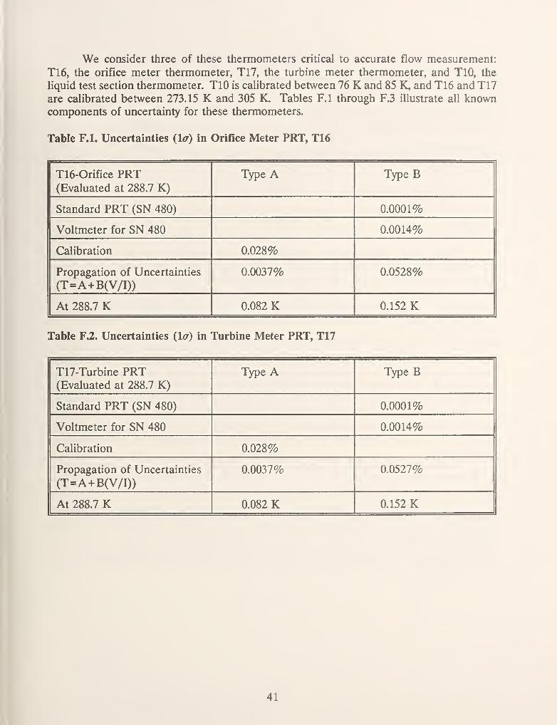
We consider three of these thermometers critical to accurate flow measurement:

T16, the orifice meter thermometer, T17, the turbine meter thermometer, and TIO, the

liquid test section thermometer. TIO is calibrated between 76 K and 85 K, and T16 and T17are calibrated between 273.15 K and 305 K. Tables F.l through F.3 illustrate all knowncomponents of uncertainty for these thermometers.

Table F.l. Uncertainties (la) in Orifice Meter PRT, T16

T16-Orifice PRT(Evaluated at 288.7 K)

Type A TypeB

Standard PRT (SN 480) 0.0001%

Voltmeter for SN 480 0.0014%

Calibration 0.028%

Propagation of Uncertainties

(T=A+B(V/I))0.0037% 0.0528%

At 288.7 K 0.082 K 0.152 K

Table F.2. Uncertainties (la) in Turbine Meter PRT, T17

T17-Turbine PRT(Evaluated at 288.7 K)

Type A Type B



Calibration 0.028%


(T=A+B(V/I))0.0037% 0.0527%

At 288.7 K 0.082 K 0.152 K

41

Table F.3. Uncertainties (la) in Liquid Test Section PRT, TIO

TlO-Liquid Test Section PRT(Evaluated at 85 K)

Type A Type B



Calibration 0.041%


(T=A+B(V/I))0.008% 0.021%

At85K 0.036 K 0.018 K

Three other thermometers provide secondary contributions to the buoyancy

corrections used in the weigh tank system. T13 measures the temperature of the liquid

collected in the weigh tank. The weigh tank temperature is used in the calculation of

density and, thereby, volume of the collected liquid. TS71 and TS72 measure the

temperature in the ullage gas surrounding the weigh tank and are used in the calculation

of ullage gas density. The buoyancy of the liquid in the ullage gas is the product of the

Hquid volume and the ullage gas density. Though accurate measurement of the ullage gas

temperature is important, its contribution to the total system uncertainty is secondary.

Thermometers T13, TS71, and TS72 are located in the catch tank and are not as

readily accessible as those located in the flow loop. For that reason, they are not calibrated

as frequently. The residual standard deviation of the original calibration of T13 was 0.4 K.

Because of the long-term stability of PRTs and the fact that T13 remains in a protected

environment free from mechanical shock, we think that the performance has not changed

significantly since the original calibration. We chose, however, to use a slightly greater value

of 0.5 K as a conservative Type B estimate of the total uncertainty in this temperature

measurement.

The manufacturer of thermometers TS71 and TS72 provided a one-point calibration

by measuring the resistance at 273.15 K. Using the manufacturer's specifications for

platinum resistance thermometers of this type, we derived a general second order calibration

curve whose independent variable is the ratio of the resistance measured at operating

temperatures to the resistance at 273.15 K. A test of this regression fit at liquid nitrogen

temperatures indicated a possible 0.5 to 0.8 K error with regards to temperatures measured

by SN 480. We will use a value of 1 K as a conservative Type B estimate of the total

uncertainty in these temperature measurements. Table F.4 lists the uncertainties associated

with these thermometers.

42

Table F.4. Uncertainties (la) in Weigh Tank and Ullage PRTs

Secondary PRTUncertainties

Type A TypeB

T13 0.5 K

TS71, TS72 1.0 K

43

APPENDIX G. UNCERTAINTIES IN DIMENSIONAL MEASUREMENTS

The uncertainties in measurement of pipe diameter and orifice diameter are listed

in Table G.l. These values will be used in the propagation of uncertainty for discharge

coefficients. The magnitudes of the measurement uncertainties are shown in parenthesis

and are evaluated at nominal values of 10.2 cm (4 in) for pipe diameter and 6.35 cm (2.5

in) for orifice diameter.

Table G.l. Dimensional Uncertainties

Dimensional Uncertainty TypeB

Pipe Diameter (0.0254 mm) 0.025%

Orifice Diameter (0.002 54 mm) 0.004%

*U.S. GOVERNMENT PRINTING OFFICE:1994-573-013/00021

44

NIST Technical Publications

Periodical

Journal of Research of the National Institute of Standards and Technology— Reports NIST research

and development in those disciplines of the physical and engineering sciences in which the Institute is

active. These include physics, chemistry, engineering, mathematics, and computer sciences. Papers

cover a broad range of subjects, with major emphasis on measurement methodology and the basic

technology underlying standardization. Also included from time to time are survey articles on topics

closely related to the Institute's technical and scientific programs. Issued six times a year.

Nonperiodicals

Monographs—Major contributions to the technical literature on various subjects related to the Institute's

scientific and technical activities.

Handbooks—Recommended codes of engineering and industrial practice (including safety codes)

developed in cooperation with interested industries, professional organizations, and regulatory bodies.

Special Publications—Include proceedings of conferences sponsored by NIST, NIST annual reports, and

other special publications appropriate to this grouping such as wall charts, pocket cards, and

bibliographies.

Applied Mathematics Series—Mathematical tables, manuals, and studies of special interest to physicists,

engineers, chemists, biologists, mathematicians, computer programmers, and others engaged in scientific

and technical work.

National Standard Reference Data Series—Provides quantitative data on the physical and chemical

properties of materials, compiled from the world's literature and critically evaluated. Developed under a

worldwide program coordinated by NIST under the authority of the National Standard Data Act (Public

Law 90-396). NOTE: The Journal of Physical and Chemical Reference Data (JPCRD) is published bi-

monthly for NIST by the American Chemical Society (ACS) and the American Institute of Physics (AIP).

Subscriptions, reprints, and supplements are available from ACS, 1155 Sixteenth St., NW, Washington,DC 20056.

Building Science Series—Disseminates technical information developed at the Institute on building

materials, components, systems, and whole structures. The series presents research results, test

methods, and performance criteria related to the structural and environmental functions and the durability

and safety characteristics of building elements and systems.

Technical Notes—Studies or reports which are complete in themselves but restrictive in their treatment

of a subject. Analogous to monographs but not so comprehensive in scope or detlnitive in treatment of

the subject area. Often serve as a vehicle for final reports of work performed at NIST under the

sponsorship of other government agencies.

Voluntary Product Standards—Developed under procedures published by the Department of Commercein Part 10, Title 15, of the Code of Federal Regulations. The standards establish nationally recognized

requirements for products, and provide all concerned interests with a basis for common understanding of

the characteristics of the products. NIST administers this program in support of the efforts of private

sector standardizing organizations.

Consumer Information Series— Practical information, based on NIST research and experience, covering

areas of interest to the consumer. Easily understandable language and illustrations provide useful

background knowledge for shopping in today's technological marketplace.

Order the above NIST publications from: Superintendent of Documents, Government Printing Office,

Washington, DC 20402.

Order the following NIST publications—FIPS and NISTIRs—from the National Technical Information

Service, Springfield, VA 22I6I.

Federal Information Processing Standards Publications (FIPS PUB)—Publications in this series

collectively constitute the Federal Inforination Processing Standards Register. The Register serves as the

official source of information in the Federal Government regarding standards issued by NIST pursuant to

the Federal Property and Administrative Services Act of 1949 as amended. Public Law 89-306 (79 Stat.

1127), and as implemented by Executive Order 11717 (38 FR 12315. dated May 11, 1973) and Part 6 of

Title 15 CFR (Code of Federal Regulations).

NIST Interagency Reports (NISTIR)—A special series of interim or final reports on work performed by

NIST for outside sponsors (both government and non-government). In general, initial distribution is

handled by the sponsor; public distribution is by the National Technical Information Service, Springfield.

VA 22161, in paper copy or microfiche form.

? o 03 WCD ~r

0) z:O NJc cn

7* O CL COZ. o* CD =ro r o- 00 _ i^

"V C O CL- w o S< —B> 3 O Q)

^^C W a.Ul o,*

00W)- o(a)

oo

COoCO

COCON)00

z cCO^ (/)

o=1 Da

5"Si

^•3C <D

^ 3CD <-

O O-h -•«

cn o^ oD 3

"SQ}

DQ.

CD

O3-

3o_

O

<