Finance and Economics Discussion SeriesDivisions of Research & Statistics and Monetary Affairs

Federal Reserve Board, Washington, D.C.

Nowcasting Indonesia

Matteo Luciani, Madhavi Pundit, Arief Ramayandi, and GiovanniVeronese

2015-100

Please cite this paper as:Luciani, Matteo, Madhavi Pundit, Arief Ramayandi, and Giovanni Veronese (2015). “Now-casting Indonesia,” Finance and Economics Discussion Series 2015-100. Washington: Boardof Governors of the Federal Reserve System, http://dx.doi.org/10.17016/FEDS.2015.100.

NOTE: Staff working papers in the Finance and Economics Discussion Series (FEDS) are preliminarymaterials circulated to stimulate discussion and critical comment. The analysis and conclusions set forthare those of the authors and do not indicate concurrence by other members of the research staff or theBoard of Governors. References in publications to the Finance and Economics Discussion Series (other thanacknowledgement) should be cleared with the author(s) to protect the tentative character of these papers.

Nowcasting Indonesia∗

Matteo Luciani Madhavi PunditFederal Reserve Board Asian Development Bank

matteo.luciani@frb.gov mpundit@adb.org

Arief Ramayandi Giovanni VeroneseAsian Development Bank Banca d’Italia

aramyandi@adb.org giovanni.veronese@bancaditalia.it

September 2015

Abstract

We produce predictions of the current state of the Indonesian economy byestimating a dynamic factor model on a dataset of eleven indicators (alsofollowed closely by market operators) over the time period 2002 to 2014.Besides the standard difficulties associated with constructing timely indica-tors of current economic conditions, Indonesia presents additional challengestypical to emerging market economies where data are often scant and unre-liable. By means of a pseudo-real-time forecasting exercise we show that ourmodel outperforms univariate benchmarks, and it does comparably with pre-dictions of market operators. Finally, we show that when quality of data islow, a careful selection of indicators is crucial for better forecast performance.

JEL codes: C32, C53, E37, O53

Keywords: Nowcasting, Dynamic Factor Models, Emerging Market Economies

∗ We would like to thank Dennis Sorino for excellent research assistance and participants ofEconomics and Research and Regional Cooperation Department, ADB seminar series for valuablecomments. The project was prepared under RDTA8951: Macroeconomic modeling for improvedeconomic assessment. This paper was written while Matteo Luciani was charge de recherchesF.R.S.-F.N.R.S., and gratefully acknowledges their financial support. Of course, any errors areour responsibility.

Disclaimer: the views expressed in this paper are those of the authors and do not necessarily reflectthe views and policies of the Asian Development Bank, of the Banca d’Italia or the Eurosystem,and of the Board of Governors or the Federal Reserve System.

1 Introduction

It is well known that macroeconomic data are released with a substantial delay.Additionally, in emerging market economies, low frequency data, i.e. annual na-tional accounts, rely on a smaller array of surveys and indicators than in advancedeconomies, and provide a partial picture of the economy. However, complete and upto date information on the current state of the economy is crucial for policy mak-ers, market participants and public institutions. Indeed, agents periodically updatetheir forecasts, and monitoring economic conditions in real-time helps them to as-sess whether the forecasts are on track or need to be revised. Similarly, the processof policymaking often requires long term projections of the economy that heavilyrely on accurate initial conditions and forecasts. Therefore, constructing timely“predictions” of current economic conditions, namely nowcasts, is of fundamentalimportance for decision making.

A lot of information is contained in economic indicators that are available on aquarterly, monthly, weekly and even daily basis, and in principle it is possible touse this information to build “predictions” of the current state of the economy.However, high frequency data in emerging market economies are often scant, noisy,released with a lag, and can have missing information. This complicates the difficulttask of real-time monitoring and decision making, particularly in an environmentwhere growth volatility is typically high, and where there is considerable uncertaintysurrounding trend growth as it may undergo changes due to rapid catching-upphases or persistent slowdowns. In other words, in addition to standard problems,constructing timely indicators on current economic conditions for emerging marketeconomies presents some extra challenges.

In this paper we focus on Indonesia, the largest economy in Southeast Asia which israpidly gaining influence in the world economy. With a number of high frequencydata indicators available and yet facing problems that commonly plague emergingeconomy datasets, Indonesia provides an interesting training case for developing anowcasting framework that can be applied to monitor other similar economies inthe region.

Two main issues emerge with regard to monitoring in real-time: how many andwhich indicators to select, and what econometric model to use to extract informationfrom the data. In this paper, we produce “predictions” of the current state of theIndonesian economy by estimating a dynamic factor model on a dataset of elevenindicators (also followed closely by market operators) over the time period 2002 to2014. Our choice of the model is based on the fact that it is parsimonious and isable to cope with missing data and mixed frequency indicators; and can potentiallybe estimated on a large number of variables. Further, since the seminal paperof Giannone et al. (2008) this model has become a standard tool for monitoringeconomic activity, as it has proved to be successful in nowcasting several economies,including emerging ones such as China (Giannone et al., 2014) and Brazil (Bragoliet al., 2014).

2

The rest of the paper proceeds as follows: Section 2 presents Indonesia’s GDPdata, and discusses the problems of having several GDP series with different baseyears, and no official seasonally adjusted data. Section 3 discusses our nowcastingprocedures. This section is divided in two parts: in the first part we describe theprocess of choosing a set of indicators that contains useful information on economicactivity, and in the second we present the application of a dynamic factor model toIndonesia’s data.

The evaluation of our model is presented in Section 4. Several results emerge.First, incorporating high frequency data in a rigorous framework leads to an im-provement in the forecast accuracy of Indonesia’s economy compared to simpleunivariate benchmarks. Second, too many variables are not always optimal for thepurpose of monitoring as they can be noisy or uninformative (see also Banburaet al., 2013; Luciani, 2014b), particularly so when the target variable, namely In-donesia’s GDP growth, has limited number of observations. A careful selection ofmeaningful variables improves the forecast performance. Third, our model does wellin predicting quarterly GDP growth when compared to private forecasters such asBloomberg, and also does well in predicting annual GDP growth when comparedto institutional forecasts of the International Monetary Fund and the Asian Devel-opment Bank.

Finally, Section 5 concludes.

2 Indonesia’s GDP data: Patterns and issues

In this Section we present Indonesia’s GDP data, and discuss a number of issues inthe data that need to be carefully tackled even before starting any monitoring pro-cess. The first is that there is no single long series available from official statisticalsources. The left hand side chart in Figure 1 plots the level of GDP at constantprices in trillion rupiah from 1993 to 2014, where the three lines refer to GDP acrossdifferent base years, 1993, 2000 and 2010 respectively. The aggregation methodol-ogy was common between the 1993 and 2000 base years, but changed from SNA1993 to SNA 2008 for the 2010 base year.1 Base changes are common for GDP dataas they can incorporate changes in the economy’s structural composition. How-ever the strikingly different slopes among the lines despite a few years of overlapsbetween series suggests that substantial revisions in data releases affect not onlythe level of GDP but also its growth rate.2 This raises questions on the composi-tion of the aggregate series and methodologies used in the construction, which isexacerbated by a lack of publicly available information on procedures used.

The right plot in Figure 1 shows the year-on-year (y-o-y) growth rate of quarterly

1 A detailed explanation of the System of National Accounts (SNA) can be found inhttp://unstats.un.org/unsd/nationalaccount/sna.asp.2 In fact even nominal GDP data for the overlapping time periods are not compara-ble between the different bases for GDP series. Data are available in Table VII.1 athttp://www.bi.go.id/en/statistik/seki/terkini/riil/Contents/Default.aspx.

3

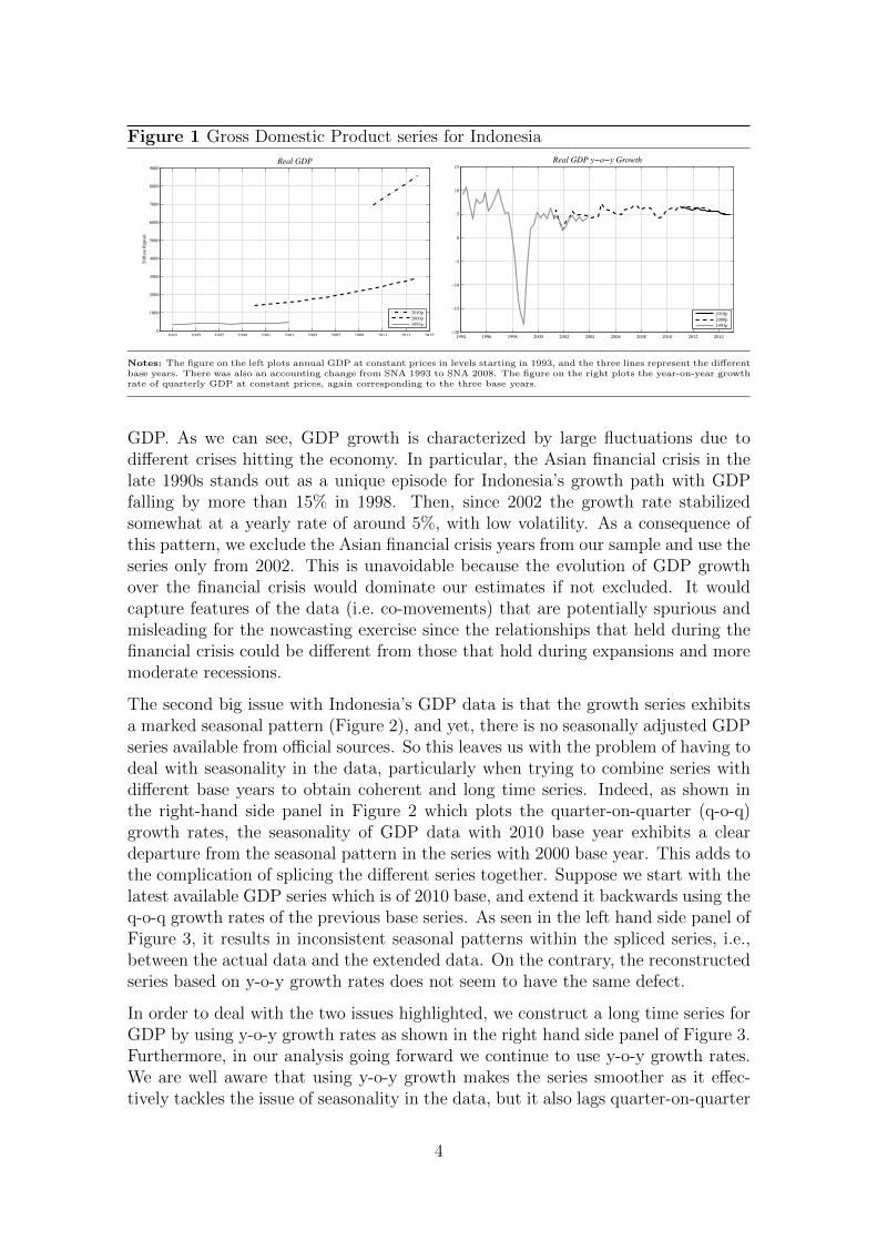
Figure 1 Gross Domestic Product series for IndonesiaT

rill

ion

Ru

pia

h

Real GDP

1993 1995 1997 1999 2001 2003 2005 2007 2009 2011 2013 20150

1000

2000

3000

4000

5000

6000

7000

8000

9000

2010p

2000p

1993p

Real GDP y−o−y Growth

1994 1996 1998 2000 2002 2004 2006 2008 2010 2012 2014−20

−15

−10

−5

0

5

10

15

2010p

2000p

1993p

Notes: The figure on the left plots annual GDP at constant prices in levels starting in 1993, and the three lines represent the differentbase years. There was also an accounting change from SNA 1993 to SNA 2008. The figure on the right plots the year-on-year growthrate of quarterly GDP at constant prices, again corresponding to the three base years.

GDP. As we can see, GDP growth is characterized by large fluctuations due todifferent crises hitting the economy. In particular, the Asian financial crisis in thelate 1990s stands out as a unique episode for Indonesia’s growth path with GDPfalling by more than 15% in 1998. Then, since 2002 the growth rate stabilizedsomewhat at a yearly rate of around 5%, with low volatility. As a consequence ofthis pattern, we exclude the Asian financial crisis years from our sample and use theseries only from 2002. This is unavoidable because the evolution of GDP growthover the financial crisis would dominate our estimates if not excluded. It wouldcapture features of the data (i.e. co-movements) that are potentially spurious andmisleading for the nowcasting exercise since the relationships that held during thefinancial crisis could be different from those that hold during expansions and moremoderate recessions.

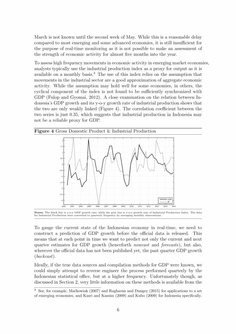
The second big issue with Indonesia’s GDP data is that the growth series exhibitsa marked seasonal pattern (Figure 2), and yet, there is no seasonally adjusted GDPseries available from official sources. So this leaves us with the problem of having todeal with seasonality in the data, particularly when trying to combine series withdifferent base years to obtain coherent and long time series. Indeed, as shown inthe right-hand side panel in Figure 2 which plots the quarter-on-quarter (q-o-q)growth rates, the seasonality of GDP data with 2010 base year exhibits a cleardeparture from the seasonal pattern in the series with 2000 base year. This adds tothe complication of splicing the different series together. Suppose we start with thelatest available GDP series which is of 2010 base, and extend it backwards using theq-o-q growth rates of the previous base series. As seen in the left hand side panel ofFigure 3, it results in inconsistent seasonal patterns within the spliced series, i.e.,between the actual data and the extended data. On the contrary, the reconstructedseries based on y-o-y growth rates does not seem to have the same defect.

In order to deal with the two issues highlighted, we construct a long time series forGDP by using y-o-y growth rates as shown in the right hand side panel of Figure 3.Furthermore, in our analysis going forward we continue to use y-o-y growth rates.We are well aware that using y-o-y growth makes the series smoother as it effec-tively tackles the issue of seasonality in the data, but it also lags quarter-on-quarter

4

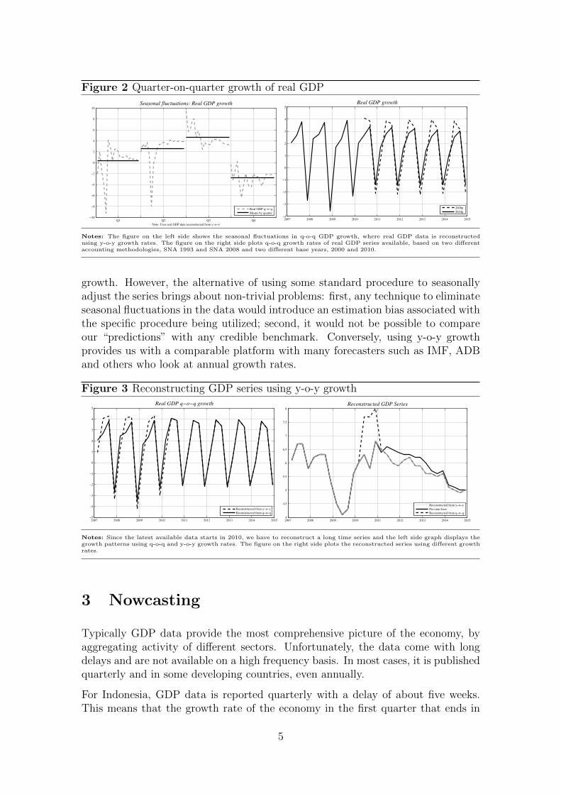
Figure 2 Quarter-on-quarter growth of real GDP

Note: Uses real GDP data reconstructed from y−o−y

Seasonal fluctuations: Real GDP growth

Q1 Q2 Q3 Q4−10

−8

−6

−4

−2

0

2

4

6

8

10

Real GDP q−o−q

Means by quarter

Real GDP growth

2007 2008 2009 2010 2011 2012 2013 2014 2015−4

−3

−2

−1

0

1

2

3

4

5

2000p

2010p

Notes: The figure on the left side shows the seasonal fluctuations in q-o-q GDP growth, where real GDP data is reconstructedusing y-o-y growth rates. The figure on the right side plots q-o-q growth rates of real GDP series available, based on two differentaccounting methodologies, SNA 1993 and SNA 2008 and two different base years, 2000 and 2010.

growth. However, the alternative of using some standard procedure to seasonallyadjust the series brings about non-trivial problems: first, any technique to eliminateseasonal fluctuations in the data would introduce an estimation bias associated withthe specific procedure being utilized; second, it would not be possible to compareour “predictions” with any credible benchmark. Conversely, using y-o-y growthprovides us with a comparable platform with many forecasters such as IMF, ADBand others who look at annual growth rates.

Figure 3 Reconstructing GDP series using y-o-y growthReal GDP q−o−q growth

2007 2008 2009 2010 2011 2012 2013 2014 2015−5

−4

−3

−2

−1

0

1

2

3

4

5

Reconstructed from y−o−y

Reconstructed from q−o−q

Reconstructed GDP Series

2007 2008 2009 2010 2011 2012 2013 2014 20154

4.5

5

5.5

6

6.5

7

7.5

8

Reconstructed from y−o−y

Previous base

Reconstructed from q−o−q

Notes: Since the latest available data starts in 2010, we have to reconstruct a long time series and the left side graph displays thegrowth patterns using q-o-q and y-o-y growth rates. The figure on the right side plots the reconstructed series using different growthrates.

3 Nowcasting

Typically GDP data provide the most comprehensive picture of the economy, byaggregating activity of different sectors. Unfortunately, the data come with longdelays and are not available on a high frequency basis. In most cases, it is publishedquarterly and in some developing countries, even annually.

For Indonesia, GDP data is reported quarterly with a delay of about five weeks.This means that the growth rate of the economy in the first quarter that ends in

5

March is not known until the second week of May. While this is a reasonable delaycompared to most emerging and some advanced economies, it is still insufficient forthe purpose of real-time monitoring as it is not possible to make an assessment ofthe strength of economic activity for almost five months into the year.

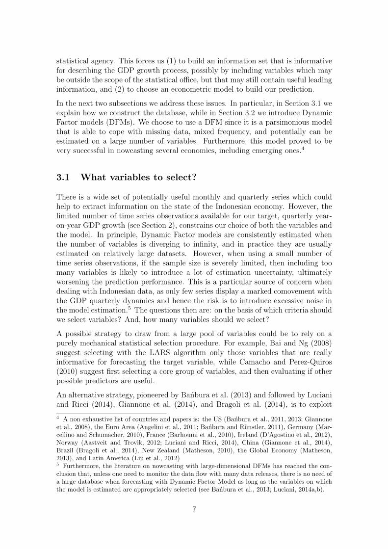
To assess high frequency movements in economic activity in emerging market economies,analysts typically use the industrial production index as a proxy for output as it isavailable on a monthly basis.3 The use of this index relies on the assumption thatmovements in the industrial sector are a good approximation of aggregate economicactivity. While the assumption may hold well for some economies, in others, thecyclical component of the index is not found to be sufficiently synchronized withGDP (Fulop and Gyomai, 2012). A close examination on the relation between In-donesia’s GDP growth and its y-o-y growth rate of industrial production shows thatthe two are only weakly linked (Figure 4). The correlation coefficient between thetwo series is just 0.35, which suggests that industrial production in Indonesia maynot be a reliable proxy for GDP.

Figure 4 Gross Domestic Product & Industrial Production

2002 2003 2004 2005 2006 2007 2008 2009 2010 2011 2012 2013 2014 2015

−3

−2.5

−2

−1.5

−1

−0.5

0

0.5

1

1.5

2

GDP

IP

Notes: The black line is y-o-y GDP growth rate, while the grey line is y-o-y growth rate of Industrial Production Index. The datafor Industrial Production were converted to quarterly frequency by averaging monthly observations.

To gauge the current state of the Indonesian economy in real-time, we need toconstruct a prediction of GDP growth before the official data is released. Thismeans that at each point in time we want to predict not only the current and nextquarter estimates for GDP growth (henceforth nowcast and forecasts), but also,wherever the official data has not been published yet, the past quarter GDP growth(backcast).

Ideally, if the true data sources and compilation methods for GDP were known, wecould simply attempt to reverse engineer the process performed quarterly by theIndonesian statistical office, but at a higher frequency. Unfortunately though, asdiscussed in Section 2, very little information on these methods is available from the

3 See, for example, Mackowiak (2007) and Raghavan and Dungey (2015) for applications to a setof emerging economies, and Kasri and Kassim (2009) and Kubo (2009) for Indonesia specifically.

6

statistical agency. This forces us (1) to build an information set that is informativefor describing the GDP growth process, possibly by including variables which maybe outside the scope of the statistical office, but that may still contain useful leadinginformation, and (2) to choose an econometric model to build our prediction.

In the next two subsections we address these issues. In particular, in Section 3.1 weexplain how we construct the database, while in Section 3.2 we introduce DynamicFactor models (DFMs). We choose to use a DFM since it is a parsimonious modelthat is able to cope with missing data, mixed frequency, and potentially can beestimated on a large number of variables. Furthermore, this model proved to bevery successful in nowcasting several economies, including emerging ones.4

3.1 What variables to select?

There is a wide set of potentially useful monthly and quarterly series which couldhelp to extract information on the state of the Indonesian economy. However, thelimited number of time series observations available for our target, quarterly year-on-year GDP growth (see Section 2), constrains our choice of both the variables andthe model. In principle, Dynamic Factor models are consistently estimated whenthe number of variables is diverging to infinity, and in practice they are usuallyestimated on relatively large datasets. However, when using a small number oftime series observations, if the sample size is severely limited, then including toomany variables is likely to introduce a lot of estimation uncertainty, ultimatelyworsening the prediction performance. This is a particular source of concern whendealing with Indonesian data, as only few series display a marked comovement withthe GDP quarterly dynamics and hence the risk is to introduce excessive noise inthe model estimation.5 The questions then are: on the basis of which criteria shouldwe select variables? And, how many variables should we select?

A possible strategy to draw from a large pool of variables could be to rely on apurely mechanical statistical selection procedure. For example, Bai and Ng (2008)suggest selecting with the LARS algorithm only those variables that are reallyinformative for forecasting the target variable, while Camacho and Perez-Quiros(2010) suggest first selecting a core group of variables, and then evaluating if otherpossible predictors are useful.

An alternative strategy, pioneered by Banbura et al. (2013) and followed by Lucianiand Ricci (2014), Giannone et al. (2014), and Bragoli et al. (2014), is to exploit

4 A non exhaustive list of countries and papers is: the US (Banbura et al., 2011, 2013; Giannoneet al., 2008), the Euro Area (Angelini et al., 2011; Banbura and Runstler, 2011), Germany (Mar-cellino and Schumacher, 2010), France (Barhoumi et al., 2010), Ireland (D’Agostino et al., 2012),Norway (Aastveit and Trovik, 2012; Luciani and Ricci, 2014), China (Giannone et al., 2014),Brazil (Bragoli et al., 2014), New Zealand (Matheson, 2010), the Global Economy (Matheson,2013), and Latin America (Liu et al., 2012)5 Furthermore, the literature on nowcasting with large-dimensional DFMs has reached the con-clusion that, unless one need to monitor the data flow with many data releases, there is no need ofa large database when forecasting with Dynamic Factor Model as long as the variables on whichthe model is estimated are appropriately selected (see Banbura et al., 2013; Luciani, 2014a,b).

7

the “revealed preferences” of professional forecasters who follow the Indonesianeconomy on the Bloomberg platform. These analysts subscribe to the Bloombergnews alert for specific data releases of the variables that they monitor, and use themto form their expectations on current and future fundamentals of Indonesia. SinceBloomberg constantly ranks the analysts’ demand for these alerts by constructinga relevance index for each macroeconomic indicator, we can select variables basedon this relevance index.6

We adopt the latter approach, since the automatic selection approach risks leadingto an unstable choice of variables in a real-time scenario.7 This instability would notonly be difficult to justify from an economic standpoint, it would also complicatethe interpretation of the forecasts’ revisions. Moreover, we also tried the automaticselection approach and the performance of our model is worse in this case thanwhen we used the revealed preference approach (see the Appendix).

It turns out that for Indonesia only a relatively small number of macroeconomicseries are tracked in real-time by the markets (see Table 1). On the one hand,there are indicators describing macroeconomic developments (e.g. the GDP itself,car sales, exports, imports and manufacturing PMI). On the other hand, giventheir direct impact on the foreign exchange and fixed income markets, analysts alsomonitor indicators that directly describe the monetary policy stance. These are thecentral bank reference interest rate as well as key monetary aggregates.

Starting from the set of indicators in Table 1 followed by business analysts weconstructed our database as follows:

1) We excluded all those indicators that either had too few observations, or we didnot manage to retrieve. This is the case of PMI for which data are available onlystarting from June 2012, and of Danareksa Consumer Confidence and MotorcycleSales for which we were not able to retrieve data.8

2) We screened each of the remaining indicators in order to understand whetherthey are followed by analysts because they convey information on the state ofthe real economy, or they are directly related to the stance of the Central Bankand its balance sheet. Therefore, since Bank of Indonesia has an inflation target,we discarded CPI, and furthermore, we also removed Foreign Reserves, and NetForeign Assets as they are mainly related to the foreign exchange policy.

3) We then excluded those variables that are the sum of other variables in thedatabase or are too similar to other series. So we kept Imports and Exports, butwe excluded Current Account; and we kept M1, but discarded M2.

6 The implicit assumption here is that since (also) based on their expectations on future funda-mentals analysts allocate their investments, they (better) know what are the relevant series tomonitor in order to form appropriate expectations on GDP growth.7 As shown by De Mol et al. (2008) since there is a lot of comovement among macroeconomicdata, the set of indicators selected with statistical criteria is extremely unstable.8 As the index compiled by Danareksa was not available to us, we experimented with the house-hold consumer confidence index compiled by the Bank of Indonesia. The latter however displaystrending pattern which appears difficult to reconcile with the state of the economy, and we hencediscarded it.

8

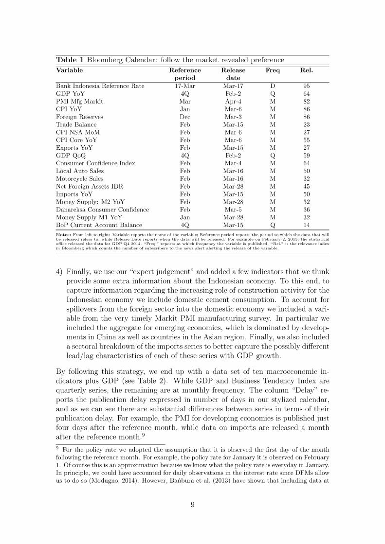
Table 1 Bloomberg Calendar: follow the market revealed preference

Variable Reference Release Freq Rel.period date

Bank Indonesia Reference Rate 17-Mar Mar-17 D 95GDP YoY 4Q Feb-2 Q 64PMI Mfg Markit Mar Apr-4 M 82CPI YoY Jan Mar-6 M 86Foreign Reserves Dec Mar-3 M 86Trade Balance Feb Mar-15 M 23CPI NSA MoM Feb Mar-6 M 27CPI Core YoY Feb Mar-6 M 55Exports YoY Feb Mar-15 M 27GDP QoQ 4Q Feb-2 Q 59Consumer Confidence Index Feb Mar-4 M 64Local Auto Sales Feb Mar-16 M 50Motorcycle Sales Feb Mar-16 M 32Net Foreign Assets IDR Feb Mar-28 M 45Imports YoY Feb Mar-15 M 50Money Supply: M2 YoY Feb Mar-28 M 32Danareksa Consumer Confidence Feb Mar-5 M 36Money Supply M1 YoY Jan Mar-28 M 32BoP Current Account Balance 4Q Mar-15 Q 14

Notes: From left to right: Variable reports the name of the variable; Reference period reports the period to which the data that willbe released refers to, while Release Date reports when the data will be released. For example on February 2, 2015, the statisticaloffice released the data for GDP Q4 2014. “Freq.” reports at which frequency the variable is published. “Rel.” is the relevance indexin Bloomberg which counts the number of subscribers to the news alert alerting the release of the variable.

4) Finally, we use our “expert judgement” and added a few indicators that we thinkprovide some extra information about the Indonesian economy. To this end, tocapture information regarding the increasing role of construction activity for theIndonesian economy we include domestic cement consumption. To account forspillovers from the foreign sector into the domestic economy we included a vari-able from the very timely Markit PMI manufacturing survey. In particular weincluded the aggregate for emerging economies, which is dominated by develop-ments in China as well as countries in the Asian region. Finally, we also includeda sectoral breakdown of the imports series to better capture the possibly differentlead/lag characteristics of each of these series with GDP growth.

By following this strategy, we end up with a data set of ten macroeconomic in-dicators plus GDP (see Table 2). While GDP and Business Tendency Index arequarterly series, the remaining are at monthly frequency. The column “Delay” re-ports the publication delay expressed in number of days in our stylized calendar,and as we can see there are substantial differences between series in terms of theirpublication delay. For example, the PMI for developing economies is published justfour days after the reference month, while data on imports are released a monthafter the reference month.9

9 For the policy rate we adopted the assumption that it is observed the first day of the monthfollowing the reference month. For example, the policy rate for January it is observed on February1. Of course this is an approximation because we know what the policy rate is everyday in January.In principle, we could have accounted for daily observations in the interest rate since DFMs allowus to do so (Modugno, 2014). However, Banbura et al. (2013) have shown that including data at

9

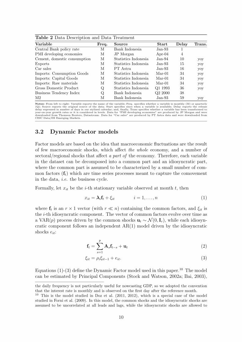
Table 2 Data Description and Data Treatment

Variable Freq. Source Start Delay Trans.Central Bank policy rate M Bank Indonesia Jan-93 1PMI developing economies M JP Morgan Apr-04 4Cement, domestic consumption M Statistics Indonesia Jan-94 10 yoyExports M Statistics Indonesia Jan-93 15 yoyCar sales M PT Astra Jan-93 16 yoyImports: Consumption Goods M Statistics Indonesia Mar-01 34 yoyImports: Capital Goods M Statistics Indonesia Mar-01 34 yoyImports: Raw materials M Statistics Indonesia Mar-01 34 yoyGross Domestic Product Q Statistics Indonesia Q1 1993 36 yoyBusiness Tendency Index Q Bank Indonesia Q2 2000 38M2 M Bank Indonesia Jan-93 59 yoy

Notes: From left to right: Variable reports the name of the variable; Freq. specifies whether a variable is monthly (M) or quarterly(Q); Source reports the original source of the data; Start specifies since when a variable is available; Delay reports the releasedelay expressed in number of days in our stylized calendar; and, finally, Trans specifies whether a variable has been transformed toyear-on-year growth rates or it is considered in levels. Data for “PMI developing economies” are produced by JP Morgan and weredownloaded from Thomson Reuters, Datastream. Data for “Car sales” are produced by PT Astra data and were downloaded fromCEIC Data/ISI Emerging Markets.

3.2 Dynamic Factor models

Factor models are based on the idea that macroeconomic fluctuations are the resultof few macroeconomic shocks, which affect the whole economy, and a number ofsectoral/regional shocks that affect a part of the economy. Therefore, each variablein the dataset can be decomposed into a common part and an idiosyncratic part,where the common part is assumed to be characterized by a small number of com-mon factors (ft) which are time series processes meant to capture the comovementin the data, i.e. the business cycle.

Formally, let xit be the i-th stationary variable observed at month t, then

xit = λift + ξit i = 1, . . . , n (1)

where ft is an r × 1 vector (with r � n) containing the common factors, and ξit isthe i-th idiosyncratic component. The vector of common factors evolve over time asa VAR(p) process driven by the common shocks ut ∼ N (0, Ir), while each idiosyn-cratic component follows an independent AR(1) model driven by the idiosyncraticshocks eit:

ft =

p∑s=1

Asft−s + ut (2)

ξit = ρiξit−1 + eit. (3)

Equations (1)-(3) define the Dynamic Factor model used in this paper.10 The modelcan be estimated by Principal Components (Stock and Watson, 2002a; Bai, 2003),

the daily frequency is not particularly useful for nowcasting GDP, so we adopted the conventionthat the interest rate is monthly and is observed on the first day after the reference month.10 This is the model studied in Doz et al. (2011, 2012), which is a special case of the modelstudied in Forni et al. (2009). In this model, the common shocks and the idiosyncratic shocks areassumed to be uncorrelated at all leads and lags, while the idiosyncratic shocks are allowed to

10

by using the Kalman Filter (Doz et al., 2011), or by maximum likelihood techniquesthrough the EM algorithm (Doz et al., 2012). In this paper we will use maximumlikelihood, and in particular we will use the EM algorithm proposed by Banburaand Modugno (2014) which can handle both mixed frequencies and missing data.

In the next section we will use the model to produce real-time predictions of In-donesian GDP growth. DFM proved very successful in real-time forecasting, andwhen used for this task they work as follows: suppose that we are at day d, andthat at date d it is available a given vintage of data: Xd. Further suppose that onthe basis of Xd we have constructed our prediction: xdit = λif

dt + et. Now, suppose

that at day d+ 1 a new data is released (eg. Exports). Based on this new piece ofinformation we can check if our stand about the business cycle is still correct or ifwe need to revised it, which is what the DFM does automatically. More specifically,at day d + 1 we have now a new vintage of data: Xd+1. Given this new vintagewe can update our estimate of the factors, fd+1

t , and hence update our prediction:

xd+1it = λif

d+1t + et

4 Empirics

4.1 The forecasting exercise

To evaluate the performance of our model, we perform a pseudo real-time out-of-sample exercise. Predictions of Indonesian GDP growth are produced according toa recursive scheme, where the first sample starts in June 2002 and ends in December2007, while the last sample starts in June 2002 and ends in December 2014. Themodel is estimated at the beginning of each quarter using only information availableas of the first day of the quarter, and then the parameters are held fixed until thenext quarter.

To perform our exercise we construct real-time vintages by replicating the patternof data availability implied by the stylized calendar (Table 2), and every time newdata are released, we update the prediction based only on information actuallyavailable at that time. We call this exercise pseudo real-time since we are not ableto track the full set of data revisions, an issue that we will discuss further later.

For the estimation, we include two factors (r = 2) and two lags (p = 2) in the VARmodel governing the evolution over time of the factors. The choice of includingtwo factors deserves a comment. First the literature on factor models has shownthat for forecasting it suffices to include a small number of factors (eg. Stock andWatson, 2002b; Forni et al., 2003). Furthermore, recent literature on small-mediumDynamic Factor models (Banbura et al., 2013; Luciani and Ricci, 2014; Giannoneet al., 2014; Bragoli et al., 2014) often include one factor only. Therefore, a natural

be cross-sectionally correlated, albeit by a limited amount (approximate factor structure). For amore comprehensive treatment of the DFM we refer the reader to the aforementioned referencesand to the survey by Luciani (2014b).

11

choice would be to follow the literature and to set r = 1. However, this literatureestimates models for q-o-q growth rates, while we are estimating a model for y-o-y growth rates, and if the model for q-o-q growth rates has one factor, then thecorresponding model for y-o-y growth rates has four factors.11 Hence, we shouldset r = 4, and, indeed, by looking at the eigenvalues of the covariance matrix wecan see clearly three/four diverging eigenvalues. However, among these three/foureigenvalues the first two clearly dominate suggesting that the other two carry mainlynoise, which motivates our choice to set r = 2.12

4.2 Comparison against Statistical Benchmark

To judge the performance of our model and to evaluate the information containedin our dataset we start by comparing our model with three benchmark models.

Our first benchmark is the naive forecast, obtained from the random walk model onGDP growth: yQt = yQt−1+εt. The second is a forecast from an autoregressive model

of order two on GDP growth: yQt = ρ1yQt−1 + ρ2y

Qt−2 + εt. Given the high persis-

tence in our target series introduced by the y-o-y transformation, these univariatebenchmarks are inherently tough competitors to match in our real-time exercise.

Our last benchmark is a bridge model (Parigi and Schlitzer, 1995). Bridge modelspredict GDP growth by using its own past plus one or more monthly indicators.13

Formally, let yt be the y-o-y GDP growth observed quarterly, i.e., at month t =3, 6, 9, . . . and let xt be a monthly variable, then the Bridge model is defined asfollows:

yt = µ+ αyt−1 + βxt + εt (4)

where xt =∑3

j=113xt−j is the monthly indicator aggregated at the quarterly fre-

quency by a simple average. In this paper, we estimated equation (4) by OLS, andwhen we have a missing observations in xt we filled it by using an AR model. Fur-thermore, the predictions from the bridge model are obtained by first estimating amodel for each monthly indicator in the database (except for the PMI series), andthen by averaging the prediction.14

Table 3 shows the Root Mean Squared Error (RMSE) at the end of each month ofthe DFM, an AR(2) model, a Random Walk, and the Bridge model. The Table is

11 Let Xt be a non-stationary variable in log-levels, and let xyt = Xt −Xt−4 be the y-o-y growthrates and xqt = Xt−Xt−1 be the q-o-q growth rates, so that xyt = xqt + xqt−1 + xqt−2 + xqt−3. Then,if the true model is xqt = λft + et, we have xyt = λ(1 +L+L2 +L3)ft + (1 +L+L2 +L3)et, whichcan be rewritten as xyt = λFt + (1 + L+ L2 + L3)et where Ft is a 4× 1 singular vector.12 The first eigenvalue account for 70% of the total variance, the second for 20%, the third for 5%,and the fourth for 3%. In the appendix we show robustness results when the model is estimatedby setting either r = 1 or r = 4.13 As pointed out by Baffigi et al. (2004), differently from DFMs, bridge models are not concernedwith particular assumption underlying the DGP of the data, but rather, the inclusion of specificexplanatory indicators is based on the simple statistical fact that they embody timely updatedinformation about the target GDP growth series.14 PMI developing countries was excluded because there are too few observations for this indicatorand the prediction is volatile.

12

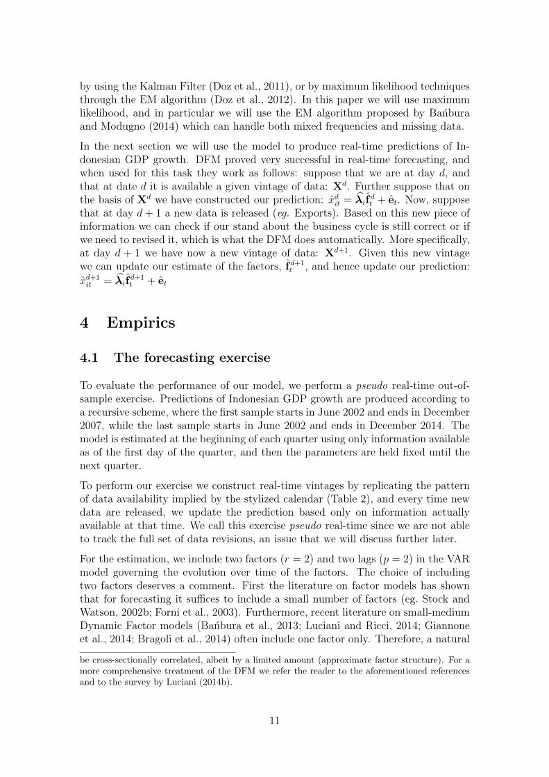
divided in three parts: the first part, labelled as “Forecast”, reports the RMSE ofthe prediction of the next quarter; the second, labelled as “Nowcast”, reports theRMSE of the prediction of the current quarter; finally, the last section, labelled as“Backcast”, reports the MSE of the prediction of the previous quarter.

As we can see from the fact that the RMSE in Table 3 are decreasing with eachmonth, the DFM is able to correctly revise its GDP prediction as more data becomesavailable. Furthermore, compared to the univariate benchmarks the RMSE of theDFM is consistently lower, up to a maximum reduction at the end of the first monthafter the reference month of 39% compared to the Autoregressive model, and of 15%compared to the Bridge model. This is an important finding since it tells us thatthere is valuable additional information in the Indonesian high frequency data thatcan be used to predict GDP growth.

Table 3 Root Mean Squared Error: End of month

Month DFM AR RW BridgeForecast 1 0.595 0.703 0.847 0.627

2 0.525 0.619 0.661 0.5673 0.467 0.619 0.661 0.536

Nowcast 1 0.441 0.609 0.666 0.4942 0.342 0.455 0.430 0.3913 0.298 0.455 0.430 0.361

Backcast 1 0.279 0.456 0.459 0.331

Notes: This table reports Root Mean Squared Error (RMSE) at the end of each month for the Dynamic Factor model (DFM),an AR(2) model, a Random Walk (RW), and the Bridge model. The upper panel labelled as “Forecast”, reports the RMSE of theprediction of the next quarter; the mid panel, labelled as “Nowcast”, reports the RMSE of the prediction of the current quarter; thebottom panel labelled as “Backcast”, reports the MSE of the prediction of the previous quarter.

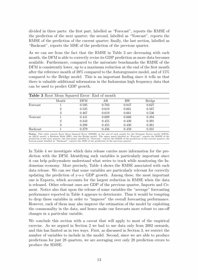
In Table 4 we investigate which data release carries more information for the pre-diction with the DFM. Identifying such variables is particularly important sinceit can help policymakers understand what series to track while monitoring the In-donesian economy. More precisely, Table 4 shows the RMSE associated with eachdata release. We can see that some variables are particularly relevant for correctlyupdating the prediction of y-o-y GDP growth. Among these, the most importantone is Exports, which accounts for the largest reduction in RMSE when the datais released. Other relevant ones are GDP of the previous quarter, Imports and Ce-ment. Notice also that upon the release of some variables the “average” forecastingperformance reported in Table 4 appears to deteriorate. Thus it would be temptingto drop these variables in order to “improve” the overall forecasting performance.However, each of them may also improve the estimation of the model by exploitingthe commonality in the data, and hence make our forecasts more robust to one-offchanges in a particular variable.

We conclude this section with a caveat that will apply to most of the empiricalexercise. As we argued in Section 2 we had to use data only from 2002 onwards,and this has limited us in two ways. First, as discussed in Section 3, we restrict thenumber of variables to include in the model. Second, since we are able to producepredictions for just 28 quarters, we are averaging over only 28 prediction errors toproduce the RMSE.

13

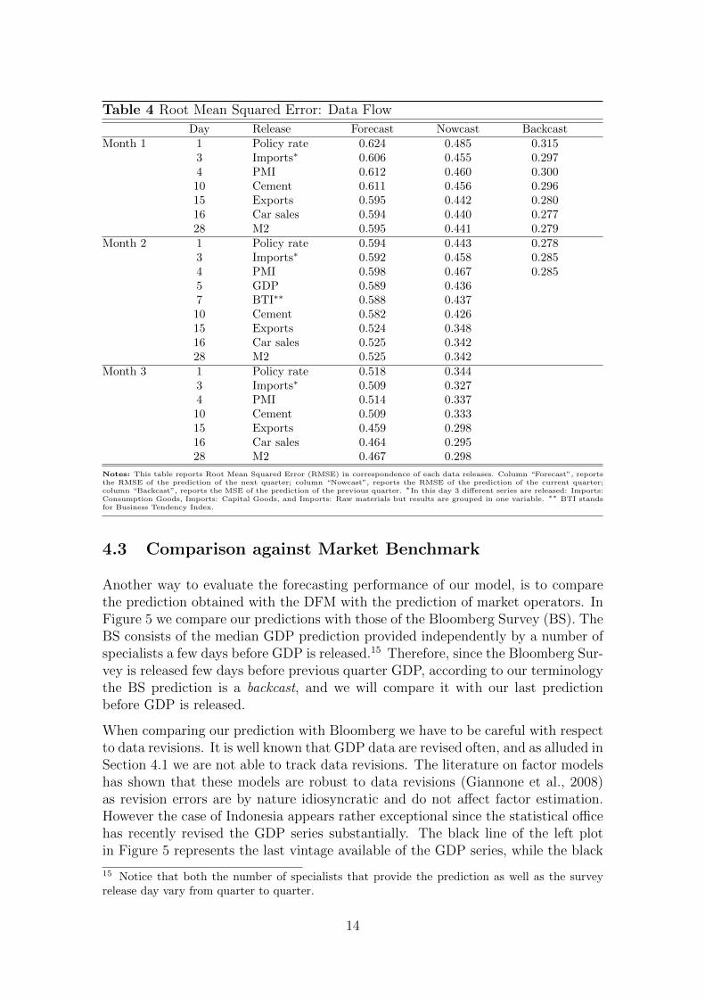
Table 4 Root Mean Squared Error: Data Flow

Day Release Forecast Nowcast BackcastMonth 1 1 Policy rate 0.624 0.485 0.315

3 Imports∗ 0.606 0.455 0.2974 PMI 0.612 0.460 0.30010 Cement 0.611 0.456 0.29615 Exports 0.595 0.442 0.28016 Car sales 0.594 0.440 0.27728 M2 0.595 0.441 0.279

Month 2 1 Policy rate 0.594 0.443 0.2783 Imports∗ 0.592 0.458 0.2854 PMI 0.598 0.467 0.2855 GDP 0.589 0.4367 BTI∗∗ 0.588 0.43710 Cement 0.582 0.42615 Exports 0.524 0.34816 Car sales 0.525 0.34228 M2 0.525 0.342

Month 3 1 Policy rate 0.518 0.3443 Imports∗ 0.509 0.3274 PMI 0.514 0.33710 Cement 0.509 0.33315 Exports 0.459 0.29816 Car sales 0.464 0.29528 M2 0.467 0.298

Notes: This table reports Root Mean Squared Error (RMSE) in correspondence of each data releases. Column “Forecast”, reportsthe RMSE of the prediction of the next quarter; column “Nowcast”, reports the RMSE of the prediction of the current quarter;column “Backcast”, reports the MSE of the prediction of the previous quarter. ∗In this day 3 different series are released: Imports:Consumption Goods, Imports: Capital Goods, and Imports: Raw materials but results are grouped in one variable. ∗∗ BTI standsfor Business Tendency Index.

4.3 Comparison against Market Benchmark

Another way to evaluate the forecasting performance of our model, is to comparethe prediction obtained with the DFM with the prediction of market operators. InFigure 5 we compare our predictions with those of the Bloomberg Survey (BS). TheBS consists of the median GDP prediction provided independently by a number ofspecialists a few days before GDP is released.15 Therefore, since the Bloomberg Sur-vey is released few days before previous quarter GDP, according to our terminologythe BS prediction is a backcast, and we will compare it with our last predictionbefore GDP is released.

When comparing our prediction with Bloomberg we have to be careful with respectto data revisions. It is well known that GDP data are revised often, and as alluded inSection 4.1 we are not able to track data revisions. The literature on factor modelshas shown that these models are robust to data revisions (Giannone et al., 2008)as revision errors are by nature idiosyncratic and do not affect factor estimation.However the case of Indonesia appears rather exceptional since the statistical officehas recently revised the GDP series substantially. The black line of the left plotin Figure 5 represents the last vintage available of the GDP series, while the black

15 Notice that both the number of specialists that provide the prediction as well as the surveyrelease day vary from quarter to quarter.

14

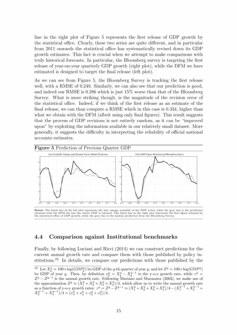
line in the right plot of Figure 5 represents the first release of GDP growth bythe statistical office. Clearly, these two series are quite different, and in particularfrom 2011 onwards the statistical office has systematically revised down its GDPgrowth estimates. This fact is crucial when we attempt to make comparisons withtruly historical forecasts. In particular, the Bloomberg survey is targeting the firstrelease of year-on-year quarterly GDP growth (right plot), while the DFM we haveestimated is designed to target the final release (left plot).

As we can see from Figure 5, the Bloomberg Survey is tracking the first releasewell, with a RMSE of 0.249. Similarly, we can also see that our prediction is good,and indeed our RMSE is 0.286 which is just 15% worse than that of the BloombergSurvey. What is more striking though, is the magnitude of the revision error ofthe statistical office. Indeed, if we think of the first release as an estimate of thefinal release, we can than compute a RMSE which in this case is 0.334, higher thanwhat we obtain with the DFM (albeit using only final figures). This result suggeststhat the process of GDP revisions is not entirely random, as it can be “improvedupon” by exploiting the information available in our relatively small dataset. Moregenerally, it suggests the difficulty in interpreting the reliability of official nationalaccounts estimates.

Figure 5 Prediction of Previous Quarter GDP

Dec07 Sep08 Jun09 Mar10 Dec10 Sep11 Jun12 Mar13 Dec13 Sep14

4

4.5

5

5.5

6

6.5

Last Available Vintage and Dynamic Factor Model Prediction

Dec07 Sep08 Jun09 Mar10 Dec10 Sep11 Jun12 Mar13 Dec13 Sep14

4

4.5

5

5.5

6

6.5

First GDP Figure Released and Bloomberg Survey

Notes: The black line of the left plot represents the last vintage available of the GDP series, while the grey line is the predictionobtained with the DFM the last day before GDP is released. The black line in the right plot represents the first figure released bythe statistical office of GDP growth, while the grey line is the median prediction from the Bloomberg Survey.

4.4 Comparison against Institutional benchmarks

Finally, by following Luciani and Ricci (2014) we can construct predictions for thecurrent annual growth rate and compare them with those published by policy in-stitutions.16 In details, we compare our predictions with those published by the

16 Let Xyq = 100×log(GDP y

q ) be GDP of the q-th quarter of year y, and let Zy = 100×log(GDP y)be GDP of year y. Then, by definition xyq = Xy

q − Xy−1q is the y-o-y growth rate, while zy =

Zy − Zy−1 is the annual growth rate. Following Mariano and Murasawa (2003), we make use ofthe approximation Zy ≈ (Xy

1 +Xy2 +Xy

3 +Xy4 )/4, which allow us to write the annual growth rate

as a function of y-o-y growth rates: zy = Zy−Zy−1 ≈ (Xy1 +Xy

2 +Xy3 +Xy

4 )/4− (Xy−11 +Xy−1

2 +Xy−1

3 +Xy−14 )/4 = (xy4 + xy3 + xy2 + xy1)/4.

15

Asian Development Bank (ADB) in the Asian Development Outlook, those pub-lished by the International Monetary Fund (IMF) in the World Economic Outlook,and the prediction by Consensus Forecast (CF).17 The ADB publishes its predic-tion of current annual GDP growth twice a year, approximately in April and in lateSeptember; also the IMF publishes twice a year its prediction but these are releasedon April and October. Predictions by CF are available each month.

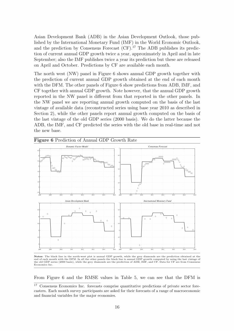
The north west (NW) panel in Figure 6 shows annual GDP growth together withthe prediction of current annual GDP growth obtained at the end of each monthwith the DFM. The other panels of Figure 6 show predictions from ADB, IMF, andCF together with annual GDP growth. Note however, that the annual GDP growthreported in the NW panel is different from that reported in the other panels. Inthe NW panel we are reporting annual growth computed on the basis of the lastvintage of available data (reconstructed series using base year 2010 as described inSection 2), while the other panels report annual growth computed on the basis ofthe last vintage of the old GDP series (2000 basis). We do the latter because theADB, the IMF, and CF predicted the series with the old base in real-time and notthe new base.

Figure 6 Prediction of Annual GDP Growth Rate

2008 2009 2010 2011 2012 2013 2014 2015

2.5

3

3.5

4

4.5

5

5.5

6

6.5

Dynamic Factor Model

2008 2009 2010 2011 2012 2013 2014 2015

4

4.5

5

5.5

6

6.5

7

Consensus Forecast

2008 2009 2010 2011 2012 2013 2014 2015

4

4.5

5

5.5

6

6.5

7

Asian Development Bank

2008 2009 2010 2011 2012 2013 2014 2015

4

4.5

5

5.5

6

6.5

7

International Monetary Fund

Notes: The black line in the north-west plot is annual GDP growth, while the grey diamonds are the prediction obtained at theend of each month with the DFM. In all the other panels the black line is annual GDP growth computed by using the last vintage ofthe old GDP series (2000 basis), while the grey diamonds are the prediction of ADB, IMF, and CF. Data for CF are from ConsensusEconomics Inc.

From Figure 6 and the RMSE values in Table 5, we can see that the DFM is

17 Consensus Economics Inc. forecasts comprise quantitative predictions of private sector fore-casters. Each month survey participants are asked for their forecasts of a range of macroeconomicand financial variables for the major economies.

16

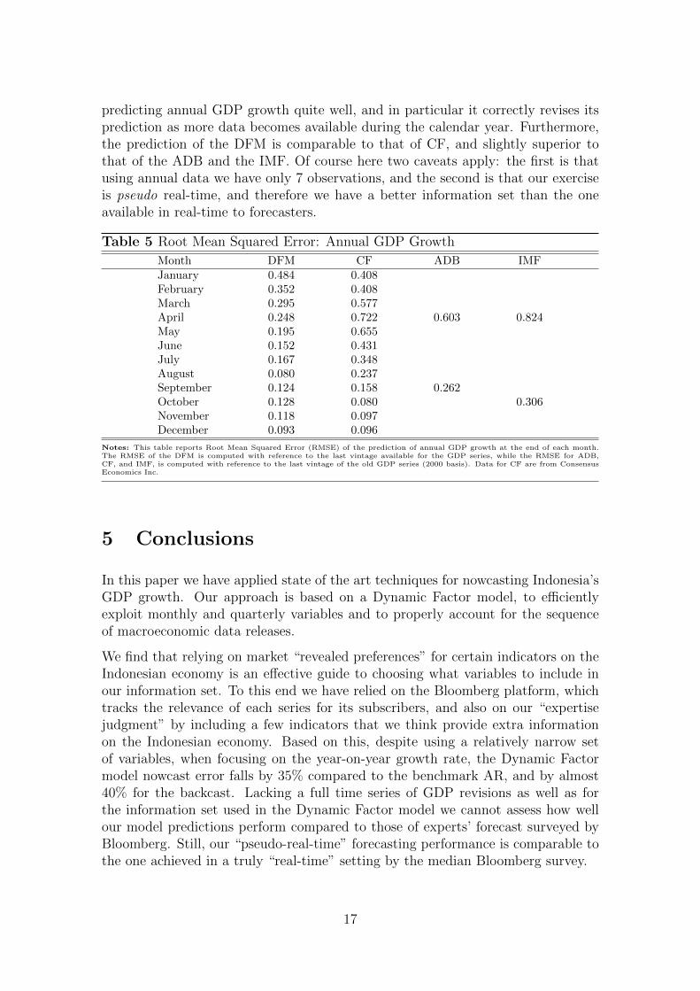
predicting annual GDP growth quite well, and in particular it correctly revises itsprediction as more data becomes available during the calendar year. Furthermore,the prediction of the DFM is comparable to that of CF, and slightly superior tothat of the ADB and the IMF. Of course here two caveats apply: the first is thatusing annual data we have only 7 observations, and the second is that our exerciseis pseudo real-time, and therefore we have a better information set than the oneavailable in real-time to forecasters.

Table 5 Root Mean Squared Error: Annual GDP Growth

Month DFM CF ADB IMFJanuary 0.484 0.408February 0.352 0.408March 0.295 0.577April 0.248 0.722 0.603 0.824May 0.195 0.655June 0.152 0.431July 0.167 0.348August 0.080 0.237September 0.124 0.158 0.262October 0.128 0.080 0.306November 0.118 0.097December 0.093 0.096

Notes: This table reports Root Mean Squared Error (RMSE) of the prediction of annual GDP growth at the end of each month.The RMSE of the DFM is computed with reference to the last vintage available for the GDP series, while the RMSE for ADB,CF, and IMF, is computed with reference to the last vintage of the old GDP series (2000 basis). Data for CF are from ConsensusEconomics Inc.

5 Conclusions

In this paper we have applied state of the art techniques for nowcasting Indonesia’sGDP growth. Our approach is based on a Dynamic Factor model, to efficientlyexploit monthly and quarterly variables and to properly account for the sequenceof macroeconomic data releases.

We find that relying on market “revealed preferences” for certain indicators on theIndonesian economy is an effective guide to choosing what variables to include inour information set. To this end we have relied on the Bloomberg platform, whichtracks the relevance of each series for its subscribers, and also on our “expertisejudgment” by including a few indicators that we think provide extra informationon the Indonesian economy. Based on this, despite using a relatively narrow setof variables, when focusing on the year-on-year growth rate, the Dynamic Factormodel nowcast error falls by 35% compared to the benchmark AR, and by almost40% for the backcast. Lacking a full time series of GDP revisions as well as forthe information set used in the Dynamic Factor model we cannot assess how wellour model predictions perform compared to those of experts’ forecast surveyed byBloomberg. Still, our “pseudo-real-time” forecasting performance is comparable tothe one achieved in a truly “real-time” setting by the median Bloomberg survey.

17

Furthermore, since our model can be used to forecast further ahead, we computealso calendar year annual growth rates. This exercise allows us to compare thetracking of our Dynamic Factor model forecasts on a smoother and medium-termindicator of Indonesia’s growth, arguably more important for policy decisions thanthe (potentially erratic) quarterly growth rate. In this case our model compares wellwith the forecasts produced by the average of private sector expectations (ConsensusForecasts) as well as by the IMF-World Economic Outlook.

Finally, our exploration into Indonesia’s data sheds light onto a lack of valuable highfrequency statistics on economic growth, as well as on deficiencies in the statisticalframework underlying national accounts.

References

Aastveit, K. A. and T. Trovik (2012). Nowcasting norwegian GDP: the role of assetprices in a small open economy. Empirical Economics 42 (1), 95–119.

Angelini, E., G. Camba-Mendez, D. Giannone, L. Reichlin, and G. Runstler (2011).Short-term forecasts of euro area gdp growth. The Econometrics Journal 14 (1),C25–C44.

Baffigi, A., R. Golinelli, and G. Parigi (2004). Bridge models to forecast the euroarea GDP. International Journal of Forecasting 20 (3), 447–460.

Bai, J. (2003). Inferential theory for factor models of large dimensions. Economet-rica 71, 135–171.

Bai, J. and S. Ng (2008). Forecasting economic time series using targeted predictors.Journal of Econometrics 146 (2), 304–317.

Banbura, M., D. Giannone, M. Modugno, and L. Reichlin (2013). Now-castingand the real-time data-flow. In G. Elliott and A. Timmermann (Eds.), Handbookof Economic Forecasting, Volume 2, pp. 195–237. Amsterdam: Elsevier-NorthHolland.

Banbura, M., D. Giannone, and L. Reichlin (2011). Nowcasting. In M. P. Clementsand D. F. Hendry (Eds.), Oxford Handbook on Economic Forecasting. New York:Oxford University Press.

Banbura, M. and M. Modugno (2014). Maximum likelihood estimation of factormodels on data sets with arbitrary pattern of missing data. Journal of AppliedEconometrics 29 (1), 133–160.

Banbura, M. and G. Runstler (2011). A look into the factor model black box: Pub-lication lags and the role of hard and soft data in forecasting GDP. InternationalJournal of Forecasting 27 (2), 333–346.

Barhoumi, K., O. Darne, and L. Ferrara (2010). Are disaggregate data useful forfactor analysis in forecasting French GDP? Journal of Forecasting 29 (1-2), 132–144.

18

Bragoli, D., L. Metelli, and M. Modugno (2014). The importance of updating:Evidence from a brazilian nowcasting model. Finance and Economics DiscussionSeries 2014-94, Federal Reserve Board.

Camacho, M. and G. Perez-Quiros (2010). Introducing the euro-sting: Short-termindicator of euro area growth. Journal of Applied Econometrics 25 (4), 663–694.

D’Agostino, A., K. McQuinn, and D. O’Brien (2012). Now-casting Irish GDP.OECD Journal: Journal of Business Cycle Measurement and Analysis 2012 (2),21–31.

De Mol, C., D. Giannone, and L. Reichlin (2008). Forecasting using a large numberof predictors: Is bayesian shrinkage a valid alternative to principal components?Journal of Econometrics 146, 318–328.

Doz, C., D. Giannone, and L. Reichlin (2011). A two-step estimator for largeapproximate dynamic factor models based on kalman filtering. Journal of Econo-metrics 164 (1), 188–205.

Doz, C., D. Giannone, and L. Reichlin (2012). A quasi maximum likelihood ap-proach for large approximate dynamic factor models. Review of Economics andStatistics 94 (4), 1014–1024.

Forni, M., D. Giannone, M. Lippi, and L. Reichlin (2009). Opening the Black Box:Structural Factor Models versus Structural VARs. Econometric Theory 25 (5),1319–1347.

Forni, M., M. Hallin, M. Lippi, and L. Reichlin (2003). Do financial variables helpforecasting inflation and real activity in the Euro Area? Journal of MonetaryEconomics 50 (6), 1243–1255.

Fulop, G. and G. Gyomai (2012). Transition of the OECD CLI system to a GDP-based business cycle target.

Giannone, D., S. Miranda Agrippino, M. Modugno, and L. Reichlin (2014). Now-casting China. mimeo.

Giannone, D., L. Reichlin, and D. Small (2008). Nowcasting: The real-time infor-mational content of macroeconomic data. Journal of Monetary Economics 55 (4),665–676.

Kasri, R. and S. H. Kassim (2009). Empirical determinants of saving in the Islamicbanks: Evidence from Indonesia. JKAU: Islamic Econ. 22 (2), 181–201.

Kubo, A. (2009). Monetary targeting and inflation: Evidence from Indonesia’spost-crisis experience. Economics Bulletin 29 (3), 1805–1813.

Liu, P., T. Matheson, and R. Romeu (2012). Real-time forecasts of economic activityfor Latin American economies. Economic Modelling 29 (4), 1090–1098.

Luciani, M. (2014a). Forecasting with approximate dynamic factor models: the roleof non-pervasive shocks. International Journal of Forecasting 30 (1), 20–29.

19

Luciani, M. (2014b). Large-dimensional dynamic factor models in real-time: Asurvey. Universite libre de Bruxelles.

Luciani, M. and L. Ricci (2014). Nowcasting Norway. International Journal ofCentral Banking 10, 215–248.

Mackowiak, B. (2007). External shocks, US monetary policy and macroeconomicfluctuations in emerging markets. Journal of Monetary Economics 54 (8), 2512–2520.

Marcellino, M. and C. Schumacher (2010). Factor MIDAS for nowcasting andforecasting with ragged-edge data: A model comparison for German GDP. OxfordBulletin of Economics and Statistics 72 (4), 518–550.

Mariano, R. S. and Y. Murasawa (2003). A new coincident index of business cyclesbased on monthly and quarterly series. Journal of Applied Econometrics 18 (4),427–443.

Matheson, T. D. (2010). An analysis of the informational content of New Zealanddata releases: The importance of business opinion surveys. Economic Mod-elling 27 (1), 304–314.

Matheson, T. D. (2013). New indicators for tracking growth in real time. Journalof Business Cycle Measurement and Analysis 2013 (1), 51–71.

Modugno, M. (2014). Now-casting inflation using high frequency data. InternationalJournal of Forecasting 29 (4), 664–675.

Parigi, G. and G. Schlitzer (1995). Quarterly forecasts of the italian business cycleby means of monthly economic indicators. Journal of Forecasting 14 (2), 117–141.

Raghavan, M. and M. Dungey (2015). Should ASEAN-5 monetary policy-makersact pre-emptively against stock market bubbles? Applied Economics 47 (11),1086–1105.

Stock, J. H. and M. W. Watson (2002a). Forecasting using principal componentsfrom a large number of predictors. Journal of the American Statistical Associa-tion 97, 1167–1179.

Stock, J. H. and M. W. Watson (2002b). Macroeconomic forecasting using diffusionindexes. Journal of Business and Economic Statistics 20 (2), 147–162.

20

A Appendix

A.1 Robustness

In this appendix we show robustness checks with respect to the number of factorsand to the composition of the dataset.

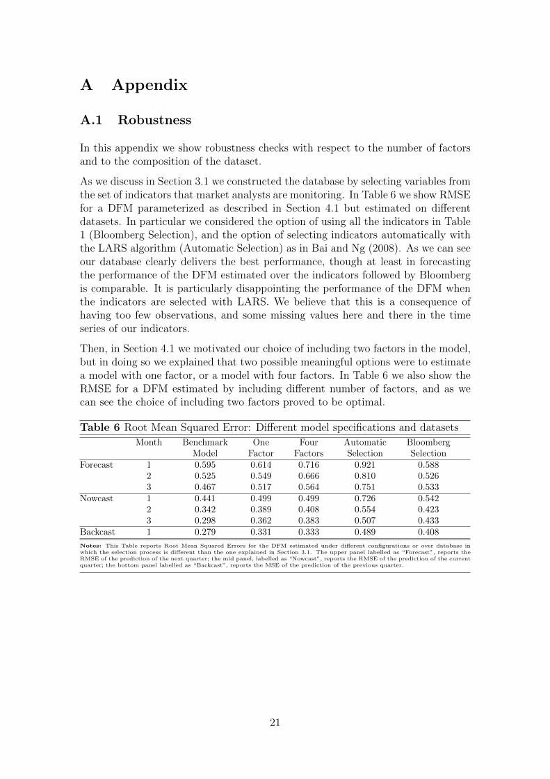
As we discuss in Section 3.1 we constructed the database by selecting variables fromthe set of indicators that market analysts are monitoring. In Table 6 we show RMSEfor a DFM parameterized as described in Section 4.1 but estimated on differentdatasets. In particular we considered the option of using all the indicators in Table1 (Bloomberg Selection), and the option of selecting indicators automatically withthe LARS algorithm (Automatic Selection) as in Bai and Ng (2008). As we can seeour database clearly delivers the best performance, though at least in forecastingthe performance of the DFM estimated over the indicators followed by Bloombergis comparable. It is particularly disappointing the performance of the DFM whenthe indicators are selected with LARS. We believe that this is a consequence ofhaving too few observations, and some missing values here and there in the timeseries of our indicators.

Then, in Section 4.1 we motivated our choice of including two factors in the model,but in doing so we explained that two possible meaningful options were to estimatea model with one factor, or a model with four factors. In Table 6 we also show theRMSE for a DFM estimated by including different number of factors, and as wecan see the choice of including two factors proved to be optimal.

Table 6 Root Mean Squared Error: Different model specifications and datasets

Month Benchmark One Four Automatic BloombergModel Factor Factors Selection Selection

Forecast 1 0.595 0.614 0.716 0.921 0.5882 0.525 0.549 0.666 0.810 0.5263 0.467 0.517 0.564 0.751 0.533

Nowcast 1 0.441 0.499 0.499 0.726 0.5422 0.342 0.389 0.408 0.554 0.4233 0.298 0.362 0.383 0.507 0.433

Backcast 1 0.279 0.331 0.333 0.489 0.408

Notes: This Table reports Root Mean Squared Errors for the DFM estimated under different configurations or over database inwhich the selection process is different than the one explained in Section 3.1. The upper panel labelled as “Forecast”, reports theRMSE of the prediction of the next quarter; the mid panel, labelled as “Nowcast”, reports the RMSE of the prediction of the currentquarter; the bottom panel labelled as “Backcast”, reports the MSE of the prediction of the previous quarter.

21