Expert Systems with Applications 39 (2012) 3413–3422

Contents lists available at SciVerse ScienceDirect

Expert Systems with Applications

journal homepage: www.elsevier .com/locate /eswa

Novelty detection for the inspection of light-emitting diodes

Fabian Timm a,b,⇑,1, Erhardt Barth b

a Pattern Recognition Company GmbH, Innovations Campus Luebeck, Maria-Goeppert-Strasse 1, D-23562 Luebeck, Germanyb University of Luebeck, Institute for Neuro- and Bioinformatics, Ratzeburger Allee 160, D-23538 Luebeck, Germany

a r t i c l e i n f o a b s t r a c t

Keywords:Defect detectionNovelty detectionLight emitting diodesFeature extractionOne-class SVMKernel PCAKernel density estimation

0957-4174/$ - see front matter � 2011 Elsevier Ltd. Adoi:10.1016/j.eswa.2011.09.029

⇑ Corresponding author at: University of LuebecBioinformatics, Ratzeburger Allee 160, D-23538 Lueb

E-mail addresses: ft@prcmail.de (F. Timm), barth@URLs: http://www.pattern-recognition-comp

http://www.inb-uni-luebeck.de (E. Barth).1 Sources can be found at http://www.inb.uni-luebe

We propose novel feature-extraction and classification methods for the automatic visual inspection ofmanufactured LEDs. The defects are located at the area of the p-electrodes and lead to a malfunctionof the LED. Besides the complexity of the defects, low contrast and strong image noise make this problemvery challenging.

For the extraction of image characteristic we compute radially-encoded features that measure discon-tinuities along the p-electrode. Therefore, we propose two different methods: the first method divides theobject into several radial segments for which mean and standard deviation are computed and the secondmethod computes mean and standard deviation along different orientations. For both methods we com-bine the features over several segments or orientations by computing simple measures such as the ratiobetween maximum and mean or standard deviation.

Since defect-free LEDs are frequent and defective LEDs are rare, we apply and evaluate different nov-elty-detection methods for classification. Therefore, we use a kernel density estimator, kernel principalcomponent analysis, and a one-class support vector machine. We further compare our results to Pear-son’s correlation coefficient, which is evaluated using an artificial reference image.

The combination of one-class support vector machine and radially-encoded segment features yields thebest overall performance by far, with a false alarm rate of only 0.13% at a 100% defect detection rate,which means that every defect is detected and only very few defect-free p-electrodes are rejected.

Our inspection system does not only show superior performance, but is also computationally efficientand can therefore be applied to further real-time applications, for example solder joint inspection. More-over, we believe that novelty detection as used here can be applied to various expert-system applications.

� 2011 Elsevier Ltd. All rights reserved.

1. Introduction

Over the last years, light emitting diodes (LED) have been em-ployed in diverse industrial products and have recently becomepopular due to the increased demand for energy-saving TVs.

Similar to Moore’s Law for transistor integration in ICs, there isthe so-called Haitz’s Law for LED devices which states that everydecade the light output level of a LED device increases by a factorof 20 and that the cost per lumen falls by a factor of 10 (Haitz, Kish,Tsao, & Nelson, 2000). It is therefore expected that LEDs will soonbe the dominant technology for many lighting applications.

Like in many other production processes an inspection of LEDsis done for quality assurance. Mainly, there are two types of

ll rights reserved.

k, Institute for Neuro- andeck, Germany.inb.uni-luebeck.de (E. Barth).any.com (F. Timm),

ck.de/tools-demos.

inspection: electrical inspection and visual inspection. The electri-cal inspection ensures correct functionality, but since an extensivestress test cannot be applied for all LEDs, defects that might cause amalfunction after a period of time cannot be detected accurately.Therefore, a visual inspection is used to detect short-term, long-term, and cosmetic defects. However, a visual inspection by humanexperts yields significant labor and production costs. Althoughhuman experts are very flexible to variations of the productionprocess, different experts may obtain different results (inter-obser-ver variability) or even one expert may obtain different results forthe same sample (intra-observer variability). Furthermore, visualinspection may lead to misjudgement due to human fatigue (Wang& Huang, 2004). These shortcomings require an automatic visualinspection for LED manufacturing.

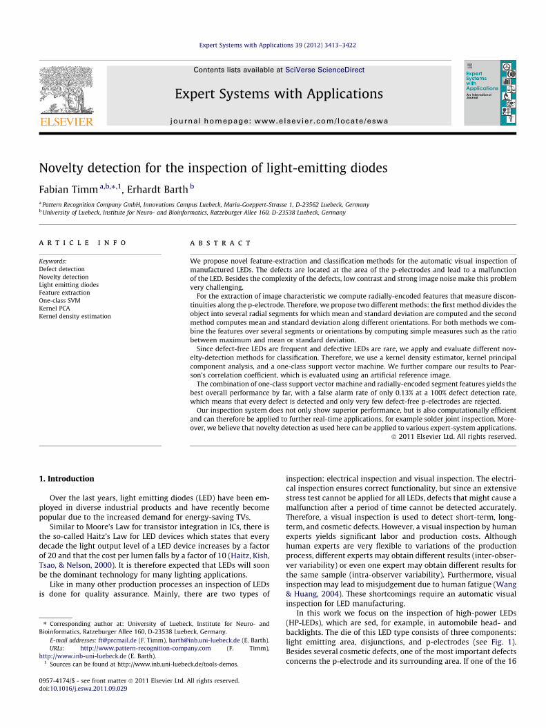
In this work we focus on the inspection of high-power LEDs(HP-LEDs), which are sed, for example, in automobile head- andbacklights. The die of this LED type consists of three components:light emitting area, disjunctions, and p-electrodes (see Fig. 1).Besides several cosmetic defects, one of the most important defectsconcerns the p-electrode and its surrounding area. If one of the 16

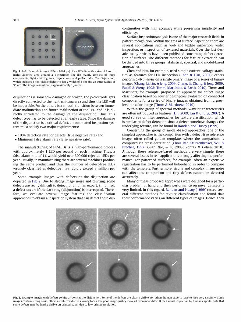
Fig. 1. Left: Example image (1024 � 1024 px) of an LED die with a size of 1 mm2.Right: Zoomed area around a p-electrode. The die mainly consists of threecomponents: light emitting area, disjunctions, and p-electrodes. The disjunction,which includes a non-visible dielectric, has a width of 8 lm and an outer radius of30 lm. The image resolution is approximately 1 lm/px.

3414 F. Timm, E. Barth / Expert Systems with Applications 39 (2012) 3413–3422

disjunctions is somehow damaged or broken, the p-electrode getsdirectly connected to the light emitting area and thus the LED willbe inoperable. Further, there is a smooth transition between imme-diate malfunction and future malfunction of the LED and it is di-rectly correlated to the damage of the disjunction. Thus, thisdefect type has to be detected at an early stage. Since the damageof the disjunction is a critical defect, an automated inspection sys-tem must satisfy two major requirements:

� 100% detection rate for defects (true negative rate) and� Minimum false alarm rate (false negative rate).

The manufacturing of HP-LEDs is a high-performance processwith approximately 1 LED per second on each machine. Thus, afalse alarm rate of 1% would yield over 300,000 rejected LEDs peryear. Usually, in manufacturing there are several machines produc-ing the same product and thus the number of defect-free LEDswrongly classified as defective may rapidly exceed a million peryear.

Some example images with defects at the disjunction aredepicted in Fig. 2. Due to strong image noise and blurring, somedefects are really difficult to detect for a human expert. Simplified,a defect occurs if the dark ring (disjunction) is interrupted. There-fore, we evaluate several image features and classificationapproaches to obtain a inspection system that can detect these dis-

Fig. 2. Example images with defects (white arrows) at the disjunction. Some of the defimages contain strong noise, others are blurred due to a wrong focus. The poor image quasome defects may be hardly visible on printed paper due to low printer resolution.

continuities with high accuracy while preserving simplicity andefficiency.

Surface inspection/analysis is one of the major research fields inpattern recognition. Within the area of surface inspection there areseveral applications such as web and textile inspection, waferinspection, or inspection of textured materials. Over the last dec-ade, many articles have been published concerning defect detec-tion of surfaces. The different methods for feature extraction canbe divided into three groups: statistical, spectral, and model-basedapproaches.

Chen and Hsu, for example, used simple current–voltage statis-tics as features for LED inspection (Chen & Hsu, 2007); othersperform blob analysis on a single binary image or a series of binaryimages (Chang, Li, Lin, & Jeng, 2009; Chang, Li, Chang, & Jeng, 2009;Fadzil & Weng, 1998; Timm, Martinetz, & Barth, 2010). Timm andMartinetz, for example, proposed an approach for defect imageclassification based on Fourier descriptors evaluated on connectedcomponents for a series of binary images obtained from a grey-level or color image (Timm & Martinetz, 2010).

Within the group of spectral methods, wavelet characteristicsare often introduced as features (Lin, 2009; Lin & Chung, 2007). Agood survey on filter approaches for texture classification, whichis similar to defect detection since a defect somehow changes theunderlying texture, can be found in Randen and Husoy (1999).

Concerning the group of model-based approaches, one of thesimplest approaches is the comparison with a defect-free referenceimage, often called golden template, where the comparison iscomputed via cross-correlation (Chou, Rao, Sturzenbecker, Wu, &Brecher, 1997; Guan, Xie, & Li, 2003; Zontak & Cohen, 2010).Although these reference-based methods are very simple, thereare several issues in real applications strongly affecting the perfor-mance. For patterned surfaces, for example, often an expensiveregistration has to be performed beforehand in order to comparewith the template. Furthermore, strong and complex image noisecan affect the comparison and tiny defects cannot be detectedaccurately.

Many of these proposed approaches were designed for a partic-ular problem at hand and their performance on novel datasets isvery limited. In this regard, Randen and Husoy (1999) tested sev-eral different methods for texture classification and found thattheir performance varies on different types of images. Hence, they

ects are clearly visible, for others human experts have to look very carefully. Somelity makes it even more difficult for a visual inspection by human experts. Note that

Fig. 3. Comparison of a two-class classifier (left) and a one-class or noveltyclassifier (right). The class of defect-free samples is denoted by squares, defectivesamples are represented by circles. Whereas the two-class classifier separates theinput space into two (indefinite) half-spaces, the one-class classifier computes aclosed subspace around the target class, which is, for this work, represented bydefect-free samples.

F. Timm, E. Barth / Expert Systems with Applications 39 (2012) 3413–3422 3415

could not identify a single approach that performs best on all data-sets, which suggests that a powerful feature-extraction method al-ways incorporates prior knowledge, especially in the case of defectdetection where the defects can be subtle and hard to identify.

For the inspection of LEDs, we propose two radially-encodedimage feature sets that describe p-electrode defects and are usedfor novelty detection. The first set consists of radial segments forwhich mean and standard deviation are evaluated, the second isbased on sampled orientations. For both we combine the seg-ment/orientation characteristics by computing simple measuressuch as maximum and mean. For comparison purposes, we alsocompute the Pearsons’s correlation coefficient with a referenceimage.

For LED inspection, neural network approaches, in particularmulti-layer perceptrons (Chang, Li, Chang, et al., 2009; Chang, Li,Lin, et al., 2009; Chen and Hsu, 2007; Lin, 2009; Lin and Chung,2007), are often used for classification. Although the performanceof these approaches is quite good, we are not aware of work thatfocusses on the original problem of novelty detection, i.e. identify-ing atypical samples. All approaches for defect detection, proposedso far, belong to the group of two-class classification approaches,where the defect-free samples describe the positive class and thedefective samples describe the negative class. But if we want todetect every defect with a minimum false alarm rate, this is aone-class or novelty-detection problem rather than a two-classproblem. The difference between a two-class and a one-class clas-sifier is shown in Fig. 3. A two-class classifier separates the inputspace into two (infinite) half spaces, whereas a one-class classifiercomputes a enclosed subspace around the target class with mini-mum volume. Especially if the other class (defective samples) isnot sampled properly and the classes are highly unbalanced, thetighter description by the one-class approach ensures a more ro-bust classification of unseen data – which might be located at areasin the input space where no data samples have been available dur-ing training. In practice this becomes very important, since theclassifier does not need to be retrained when new types of defectsoccur. This curse of imbalanced training sets has been addressed in

Fig. 4. The preprocessing steps from left to right: rough estimation of the centres by plaimage using Otsu’s method, and determining the correct centre by applying the CHT on

Japkowicz and Stephen (2002), Kubat and Matwin (1997) andRaskutti and Kowalczyk (2004), for example.

In this work, we use three different approaches for noveltydetection: kernel density estimation (Parzen, 1962), kernel princi-pal component analysis (Hoffmann, 2007; Schölkopf, Smola, &Müller, 1998), and one-class support vector machine (Labusch,Timm, & Martinetz, 2008; Schölkopf, Platt, Shawe-Taylor, Smola,& Williamson, 2001; Tax & Duin, 2004, 1999). We analyse thesemethods according to their false alarm rate at perfect (100%) defectdetection rate and we evaluate the performance for differentparameters.

2. Methods

First of all, we describe the steps of preprocessing made to de-tect the p-electrodes and its surrounding area. Then we motivateand describe the computation of image features for the defectdetection of LEDs. Finally, we will explain the different approachesfor novelty detection in detail.

2.1. Preprocessing

There are 16 p-electrodes per die placed in a 4-by-4 grid. Sincethe position of this 4-by-4 grid varies only slightly, we first esti-mate the rough position of the p-electrodes. Then, we localisethe correct centre of the p-electrodes by computing the binary im-age via Otsu’s method (Otsu, 1979) and performing a circularHough transform (CHT) afterwards (Kimme, Ballard, & Sklansky,1975), see also Fig. 4. Based on the estimated centre we extract aregion of 100 � 100 pixels to cover the p-electrode and itssurroundings.

2.2. Feature extraction

For feature extraction we use Pearson’s correlation coefficientwith a reference image and two novel radially-encoded feature setsusing segments and sampled orientations.

2.2.1. Pearson’s correlation coefficientThe comparison of an input image with a reference image is

very intuitive, since this is similar to what a human expert will per-form. Based on a number of defect-free samples a human expertwill notice a defect as a deviation from already known samples.

Pearson’s correlation coefficient is often used for template/ref-erence matching, since it is more robust to variations concerningbrightness and noise than just a simple correlation. Assume thatthe template T and the image I have the same width W and heightH, then Pearson’s correlation coefficient c is defined as:

cðI; TÞ ¼ 1rIrT

XH

i¼1

XWj¼1

ðIði; jÞ � lIÞðTði; jÞ � lTÞ; ð1Þ

where lI and lT are the image mean and the template mean,respectively, and rI, rT are the standard deviations of the image

cing a virtual grid on the die, extraction of the grid elements, computing the binarythe contour points.

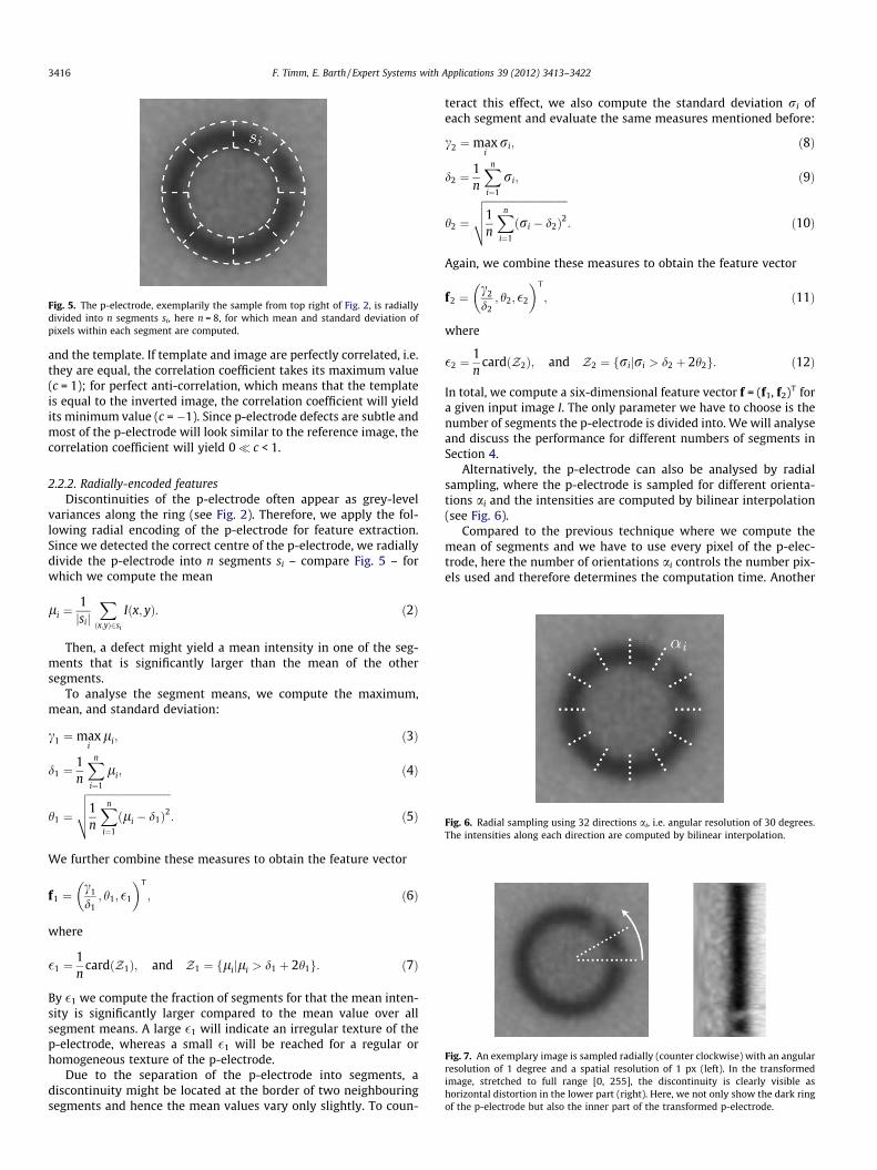
Fig. 5. The p-electrode, exemplarily the sample from top right of Fig. 2, is radiallydivided into n segments si, here n = 8, for which mean and standard deviation ofpixels within each segment are computed.

ig. 7. An exemplary image is sampled radially (counter clockwise) with an angularsolution of 1 degree and a spatial resolution of 1 px (left). In the transformedage, stretched to full range [0, 255], the discontinuity is clearly visible as

orizontal distortion in the lower part (right). Here, we not only show the dark ringof the p-electrode but also the inner part of the transformed p-electrode.

Fig. 6. Radial sampling using 32 directions ai, i.e. angular resolution of 30 degrees.The intensities along each direction are computed by bilinear interpolation.

3416 F. Timm, E. Barth / Expert Systems with Applications 39 (2012) 3413–3422

and the template. If template and image are perfectly correlated, i.e.they are equal, the correlation coefficient takes its maximum value(c = 1); for perfect anti-correlation, which means that the templateis equal to the inverted image, the correlation coefficient will yieldits minimum value (c = �1). Since p-electrode defects are subtle andmost of the p-electrode will look similar to the reference image, thecorrelation coefficient will yield 0� c < 1.

2.2.2. Radially-encoded featuresDiscontinuities of the p-electrode often appear as grey-level

variances along the ring (see Fig. 2). Therefore, we apply the fol-lowing radial encoding of the p-electrode for feature extraction.Since we detected the correct centre of the p-electrode, we radiallydivide the p-electrode into n segments si – compare Fig. 5 – forwhich we compute the mean

li ¼1jsij

Xðx;yÞ2si

Iðx; yÞ: ð2Þ

Then, a defect might yield a mean intensity in one of the seg-ments that is significantly larger than the mean of the othersegments.

To analyse the segment means, we compute the maximum,mean, and standard deviation:

c1 ¼ maxi

li; ð3Þ

d1 ¼1n

Xn

i¼1

li; ð4Þ

h1 ¼

ffiffiffiffiffiffiffiffiffiffiffiffiffiffiffiffiffiffiffiffiffiffiffiffiffiffiffiffiffiffiffiffi1n

Xn

i¼1

ðli � d1Þ2vuut : ð5Þ

We further combine these measures to obtain the feature vector

f1 ¼c1

d1; h1; �1

� �T

; ð6Þ

where

�1 ¼1n

cardðZ1Þ; and Z1 ¼ flijli > d1 þ 2h1g: ð7Þ

By �1 we compute the fraction of segments for that the mean inten-sity is significantly larger compared to the mean value over allsegment means. A large �1 will indicate an irregular texture of thep-electrode, whereas a small �1 will be reached for a regular orhomogeneous texture of the p-electrode.

Due to the separation of the p-electrode into segments, adiscontinuity might be located at the border of two neighbouringsegments and hence the mean values vary only slightly. To coun-

teract this effect, we also compute the standard deviation ri ofeach segment and evaluate the same measures mentioned before:

c2 ¼maxi

ri; ð8Þ

d2 ¼1n

Xn

i¼1

ri; ð9Þ

h2 ¼

ffiffiffiffiffiffiffiffiffiffiffiffiffiffiffiffiffiffiffiffiffiffiffiffiffiffiffiffiffiffiffiffi1n

Xn

i¼1

ðri � d2Þ2vuut : ð10Þ

Again, we combine these measures to obtain the feature vector

f2 ¼c2

d2; h2; �2

� �T

; ð11Þ

where

�2 ¼1n

cardðZ2Þ; and Z2 ¼ frijri > d2 þ 2h2g: ð12Þ

In total, we compute a six-dimensional feature vector f = (f1, f2)T fora given input image I. The only parameter we have to choose is thenumber of segments the p-electrode is divided into. We will analyseand discuss the performance for different numbers of segments inSection 4.

Alternatively, the p-electrode can also be analysed by radialsampling, where the p-electrode is sampled for different orienta-tions ai and the intensities are computed by bilinear interpolation(see Fig. 6).

Compared to the previous technique where we compute themean of segments and we have to use every pixel of the p-elec-trode, here the number of orientations ai controls the number pix-els used and therefore determines the computation time. Another

Freimh

Fig. 9. Estimated density model for toy data and varied bandwidth. For small r theestimated model is very sensitive (top panel), whereas a large r results in asmoothed model such that the bimodal nature of the underlying distribution iswashed out (bottom panel). A good density model is obtained for some interme-diate r (middle panel).

F. Timm, E. Barth / Expert Systems with Applications 39 (2012) 3413–3422 3417

advantage of this sampling technique is that it implicitly performsan image transform – the p-electrode is unrolled or transformed topolar coordinates (see Fig. 7). Hence, we can use the transformedimage to compute the features described in (6) and (11) by com-puting the mean and standard deviation row-by-row.

A comparison concerning the number of involved pixels betweenthe two radial encoded feature sets is shown in Fig. 8. For few orien-tations the sampling technique employs only a fraction of pixelscompared to the separation into segments and it grows linearly inthe number of orientations. Both approaches use the same numberof pixels at around 130–140 segments/orientations; above this valuethe sampling technique performs an oversampling.

2.3. Novelty detection

Novelty detection is the identification of atypical samples – of-ten called outliers – that differ from the target class. Novelty detec-tion is an extremely challenging task, since there is only sufficientinformation available about the target class, the outlier class is (al-most) unknown. Especially in biomedical applications such as can-cer detection or tissue classification novelty-detection methodshave become very important, since samples from healthy patientsare frequent but negative samples are rare. However, in industrialapplications two-class classification methods are commonly ap-plied although the underlying problem is the detection of atypicalexamples or outliers. Therefore, we apply and evaluate differentnovelty-detection methods for the detection of atypical p-elec-trodes. We will use a kernel density estimator (Duda & Hart,1973) and a one-class support vector machine (Schölkopf et al.,2001; Tax & Duin, 1999, 2004) since both approaches yield accu-rate results on benchmark datasets as well as real-world problems(Labusch et al., 2008; Timm & Martinetz, 2010; Timm et al., 2010).Further, we apply an approach based on principal component anal-ysis that was proposed recently (Hoffmann, 2007).

A good survey of novelty-detection methods was published byMarkou and Singh (2003, 2003), where they discuss statistical ap-proaches in the first part and neural network approaches in thesecond part.

Since novelty-detection methods are rarely used in industrialapplications, we will describe the methods used for the defectdetection of p-electrodes in detail.

2.3.1. Kernel density estimatorOne of the most important non-parametric approaches for nov-

elty detection is the so-called kernel density estimator (KDE) (Duda& Hart, 1973) or Parzen estimator (Parzen, 1962) that estimates theunderlying density. Hence, we can reject data samples as outliers,if their estimated probability density is below a certain threshold.

The estimated probability density function at x can be writtenas

pðxÞ ¼ 1n

Xn

i¼1

1m

kx� xi

h

� �; ð13Þ

Fig. 8. Comparison of both feature-extraction methods concerning the number ofpixels involved for different parameters.

where h is a smoothing parameter, k some kernel function, and m anormalisation factor such thatZ

pðxÞdx ¼ 1: ð14Þ

A common choice for the kernel function is the Gaussian, whichyields the following kernel density model

pðxÞ ¼ 1n

Xn

i¼1

1

ð2pr2Þp=2 exp �kx� xik2

2r2

!; ð15Þ

where r represents the standard deviation of the Gaussian. Thus,the density model is determined by placing a Gaussian over eachdata point, then adding up the contributions over all data samples,and dividing by the number of samples for correct normalisation. InFig. 9 the density model is applied to toy data with different valuesof r. Clearly, the parameter strongly influences the estimated modeland can deliver very smooth results for large r, but also results thatare very sensitive to noise at small r. There are several techniquesfor computing a proper r such as maximisation of the log likelihoodor cross validation. Since we have some defect samples available fortraining, we will use cross validation for obtaining r in order tominimise the generalisation error of both classes.

One of the main advantages of KDE is that there is no explicittraining phase, but on the other hand KDE requires storage of thewhole training set and the cost of evaluating the density of anew sample grows linearly with the size of data set. However,there are techniques that reduce the amount of data samplesneeded for a good approximation of the density, for example re-duced set methods or clustering methods.

2.3.2. Kernel PCAPrincipal component analysis (PCA) is a standard tool for data

analysis, feature extraction and dimension reduction. If the inputvariables are linearly related to each other, the direction with max-imum variance describes the data best and is therefore called firstprincipal component (see Fig. 10).

If the input variables are nonlinearly related to each other, thedata samples are transformed from the input space into a featurespace of higher dimensionality. It is assumed that within this fea-ture space the data samples are then linearly related and standardprincipal component analysis can be performed, therefore it is

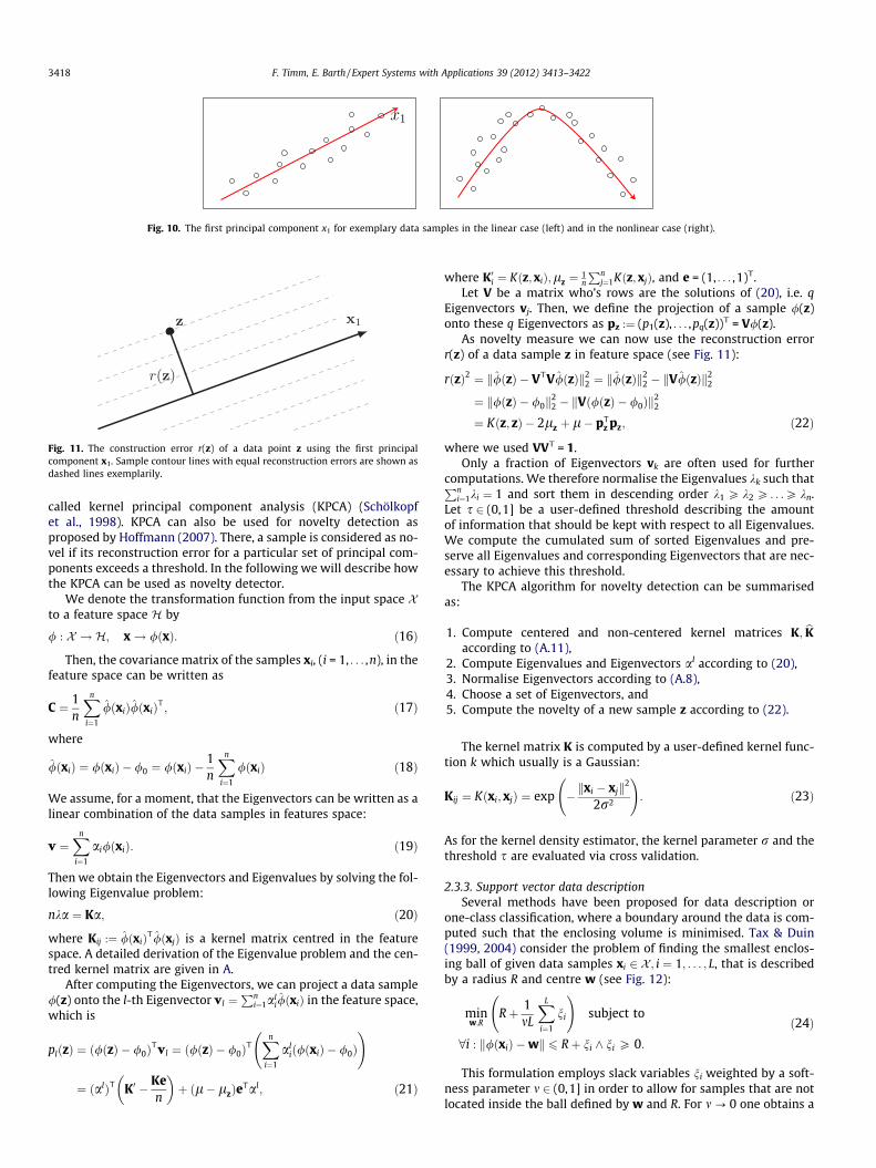
Fig. 10. The first principal component x1 for exemplary data samples in the linear case (left) and in the nonlinear case (right).

Fig. 11. The construction error r(z) of a data point z using the first principalcomponent x1. Sample contour lines with equal reconstruction errors are shown asdashed lines exemplarily.

3418 F. Timm, E. Barth / Expert Systems with Applications 39 (2012) 3413–3422

called kernel principal component analysis (KPCA) (Schölkopfet al., 1998). KPCA can also be used for novelty detection asproposed by Hoffmann (2007). There, a sample is considered as no-vel if its reconstruction error for a particular set of principal com-ponents exceeds a threshold. In the following we will describe howthe KPCA can be used as novelty detector.

We denote the transformation function from the input space Xto a feature space H by

/ : X ! H; x! /ðxÞ: ð16Þ

Then, the covariance matrix of the samples xi, (i = 1, . . . ,n), in thefeature space can be written as

C ¼ 1n

Xn

i¼1

/̂ðxiÞ/̂ðxiÞT; ð17Þ

where

/̂ðxiÞ ¼ /ðxiÞ � /0 ¼ /ðxiÞ �1n

Xn

i¼1

/ðxiÞ ð18Þ

We assume, for a moment, that the Eigenvectors can be written as alinear combination of the data samples in features space:

v ¼Xn

i¼1

ai/ðxiÞ: ð19Þ

Then we obtain the Eigenvectors and Eigenvalues by solving the fol-lowing Eigenvalue problem:

nka ¼ Ka; ð20Þ

where Kij :¼ /̂ðxiÞT/̂ðxjÞ is a kernel matrix centred in the featurespace. A detailed derivation of the Eigenvalue problem and the cen-tred kernel matrix are given in A.

After computing the Eigenvectors, we can project a data sample/(z) onto the l-th Eigenvector vl ¼

Pni¼1al

i/̂ðxiÞ in the feature space,which is

plðzÞ ¼ ð/ðzÞ � /0ÞTvl ¼ ð/ðzÞ � /0Þ

TXn

i¼1

alið/ðxiÞ � /0Þ

!

¼ ðalÞT K0 � Ken

� �þ ðl� lzÞeTal; ð21Þ

where K0i ¼ Kðz;xiÞ;lz ¼ 1n

Pnj¼1Kðz;xjÞ, and e = (1, . . . ,1)T.

Let V be a matrix who’s rows are the solutions of (20), i.e. qEigenvectors vj. Then, we define the projection of a sample /(z)onto these q Eigenvectors as pz :¼ (p1(z), . . . ,pq(z))T = V/(z).

As novelty measure we can now use the reconstruction errorr(z) of a data sample z in feature space (see Fig. 11):

rðzÞ2 ¼ k/̂ðzÞ � VTV/̂ðzÞk22 ¼ k/̂ðzÞk

22 � kV/̂ðzÞk2

2

¼ k/ðzÞ � /0k22 � kVð/ðzÞ � /0Þk

22

¼ Kðz; zÞ � 2lz þ l� pTz pz; ð22Þ

where we used VVT = 1.Only a fraction of Eigenvectors vk are often used for further

computations. We therefore normalise the Eigenvalues kk such thatPni¼1ki ¼ 1 and sort them in descending order k1 P k2 P . . .P kn.

Let s 2 (0,1] be a user-defined threshold describing the amountof information that should be kept with respect to all Eigenvalues.We compute the cumulated sum of sorted Eigenvalues and pre-serve all Eigenvalues and corresponding Eigenvectors that are nec-essary to achieve this threshold.

The KPCA algorithm for novelty detection can be summarisedas:

1. Compute centered and non-centered kernel matrices K; bKaccording to (A.11),

2. Compute Eigenvalues and Eigenvectors al according to (20),3. Normalise Eigenvectors according to (A.8),4. Choose a set of Eigenvectors, and5. Compute the novelty of a new sample z according to (22).

The kernel matrix K is computed by a user-defined kernel func-tion k which usually is a Gaussian:

Kij ¼ Kðxi; xjÞ ¼ exp �kxi � xjk2

2r2

!: ð23Þ

As for the kernel density estimator, the kernel parameter r and thethreshold s are evaluated via cross validation.

2.3.3. Support vector data descriptionSeveral methods have been proposed for data description or

one-class classification, where a boundary around the data is com-puted such that the enclosing volume is minimised. Tax & Duin(1999, 2004) consider the problem of finding the smallest enclos-ing ball of given data samples xi 2 X ; i ¼ 1; . . . ; L, that is describedby a radius R and centre w (see Fig. 12):

minw;R

Rþ 1mL

XL

i¼1

ni

!subject to

8i : k/ðxiÞ �wk 6 Rþ ni ^ ni P 0:

ð24Þ

This formulation employs slack variables ni weighted by a soft-ness parameter m 2 (0,1] in order to allow for samples that are notlocated inside the ball defined by w and R. For m ? 0 one obtains a

Fig. 12. Support vector data description, as proposed by Tax and Duin (1999, 2004), applied to toy data without a kernel (left) and using a Gaussian kernel (right). Supportvectors are indicated by an additional circle. Note that centre and radius cannot be depicted in the input space when a kernel function is applied (right).

F. Timm, E. Barth / Expert Systems with Applications 39 (2012) 3413–3422 3419

solution where all samples are located inside the hypersphere,whereas for m ? 1 a large fraction of samples are located outsidethe sphere. Here / denotes a mapping of the data samples to somefeature space, similar to (16).

Schölkopf et al. (2001) deal with data description as a two-classclassification problem, where the other class is represented by theorigin. They consider the problem of finding the hyperplane w thatseparates the data samples from the origin with maximum dis-tance q:

minw;n;q

12kwk2 þ 1

mL

XL

i¼1

ni � q

!subject to

8i : wT/ðxiÞP q� ni ^ ni P 0:

ð25Þ

Again, the behaviour of m remains the same – for m ? 0 one obtainsthe hard-margin solution that enforces correct classification of alltraining samples.

Furthermore, Schölkopf et al. showed that (24) and (25) turnout to be equivalent, if the /(xi) lie on the surface of a sphereand if they are linearly separable form the origin in feature space.

A kernel satisfying these conditions is, for example, the Gauss-ian kernel

Kðx; yÞ ¼ h/ðxÞ;/ðyÞi ¼ exp�kx� yk2

2r2

!: ð26Þ

Usually only a fraction of data samples influence the estimatedboundary – they are called support vectors. There are two typesof support vectors, the first are located on the boundary of the sur-face and the others are located outside the sphere (see Fig. 12). Theradius R in (24) and the margin q in (25) can then easily be com-puted by choosing a support vector on the boundary.

Whereas the above mentioned approaches rely on a 1-normslack term, also a 2-norm slack term is reasonable. In this case,the optimisation problem can be expressed as

minw;n

12kwk2

2 þC2

XL

i¼1

n2i

!subject to

8i : wT/ðxiÞP 1� ni; and ni P 0;

ð27Þ

where the parameter C 2 (0,1) controls the softness (similar to m in(24) and (25)).

By setting the partial derivatives to zero and rearranging, weobtain the dual optimisation problem:

mina

Piai � 1

2

Pi;j

aiajK�ðxi; xjÞ

!s:t:

8i : ai P 0:

ð28Þ

Here, K�ðxi;xjÞ ¼ Kðxi; xjÞ þdij

C defines the modified kernel and dij isKronecker’s delta. Henceforth, the original and the modified kernelwill be denoted by K and K⁄ respectively.

Labusch et al. (2008) proposed an iterative approach, calledOneClassMaxMinOver (OMMO), for solving problem (28), in whichthey only apply simple mathematical operations (see Alg. 1).OMMO converges to the support vector solution with at leastOð1=

ffiffitpÞ where t is the number of iterations (Labusch et al.,

2008). A new sample x is classified by f ðxÞ ¼ signðP

iai

Kðx;xiÞ � 1Þ.

Algorithm 1. OneClassMaxMinOver

a 0;for t 0, . . . , tmax do

s K⁄a;imin arg minisi;imax arg maxi;ai>0si;aimin

aiminþ 2;

aimax aimax � 1;ends K⁄a;q minisi;a a/q;

3. Experiments

We have collected 53 images of LEDs for which we extractedthe p-electrodes that were labelled by three experts yielding767 defect-free and 81 defective p-electrodes. Note that someof the defects are hardly visible (compare Fig. 2); therefore wetreated a p-electrode as defective, if at least one expert recog-nized a defect.

In pattern recognition applications, often a receiver operatingcharacteristic (ROC) is used to demonstrate the system’s perfor-mance or to compare different models and select the best modelaccording to some user-defined criteria. In general, a ROC analysisis based on the four outcomes that can be described by a 2 � 2 con-fusion matrix C:

C ¼true positive false positive

false negative true negative

!;

with the definitions:

FiB wlo(ri

3420 F. Timm, E. Barth / Expert Systems with Applications 39 (2012) 3413–3422

g. 13. Examples of ROC scenarioith same EER and AUC but diffe

wer AUC and EER than curve B,ght).

predicted label

s where dashed line is the EER. Twrent FAR at 100% detection rate (lebut B yields a lower FAR at 100%

true label

true positive

+1 +1 false positive �1 +1 true negative �1 �1 false negative +1 �1

Fig. 14. Artificial image of a p-electrode used as reference.

For the novelty-detection methods of the previous section, theelements of the confusion matrix are evaluated by varying thediscrimination threshold that is:

� For KDE the estimated density p(x), see (15),� For KPCA the reconstruction error r(x), see (22), and� For OMMO the distance to the hyperplane in feature space, i.e.

dðxÞ ¼P

iai Kðx;xiÞ � 1.

By using the elements of the confusion matrix we can visual-ise different ratios, e.g. true positive rate vs. false positive rate.Since we need to obtain a system that can perfectly detectdefects, we are interested in the ratio of true negative rate vs.false negative rate and we will refer to this in the following bydetection rate (of defects) and false alarm rate (for defect-freesamples).

In many applications, model comparison or model selectionbased on ROC analysis is performed using the equal error rate(EER) or the area under curve (AUC), where EER is defined asthe location on the ROC curve at which both detection rate andfalse alarm rate (FAR) obtain the same error rate. Hanley &McNeil (1982) showed that the AUC can be interpreted as theprobability that a randomly chosen negative sample is correctlyclassified or ranked with a greater suspicion than a randomlychosen positive sample; therefore the AUC is strongly connectedto the nonparametric Wilcoxon statistic. However, there areROC scenarios for which the EER and the AUC are not appropriatemeasures, especially for applications that require 100% detectionrate for defects and minimum false alarm rate. For this case,two ROC scenarios are shown in Fig. 13, where minimising theEER or AUC does not necessarily lead to a minimum false alarmrate. For the experiments, we therefore evaluate the ROC curveat 100% detection rate and perform model selection by minimis-ing FAR.

We normalise each feature to [�1,+1] and we perform 10-foldcross validation (Stone, 1974) for obtaining the best parameterfor each novelty-detection method, e.g. softness C and bandwidthr for OMMO. Moreover, we apply a Wilcoxon sign rank test to ana-lyse if the results are statistically significant.

We compare the three novelty-detection methods with respectto different feature sets:

o curves A andft). Curve A hasdetection rate

� Pearson’s correlation coefficient,� Statistics of mean values for different number of radial seg-

ments (s 2 {8, 16, 32, 64, 128, 256}), and� Statistics of mean values for different number of sampled orien-

tations (a 2 {8, 16, 32, 64, 128, 256}).

Furthermore, we analyse the performance for different parame-ter values of both radial encoding feature-extraction methods.

For the the computation of the correlation coefficient, we can-not use the average defect-free p-electrode image as a template,since the images contain strong noise of different types which willproduce a bias towards one of the noise types. Instead of smooth-ing the images to reduce the noise, we created an artificial image ofthe p-electrode, see Fig. 14, which then serves as reference.

Since the width of the ring is approximately 8 pixels (see Fig. 1),we compute 8 pixels for each orientation by using bilinear interpo-lation which corresponds to a spatial resolution of 1px or 1lmrespectively.

4. Results and discussion

The results for the correlation coefficient are depicted in Fig. 15.Since we only tested one single feature in this scenario, evaluatingthe ROC curve will already yield the best threshold for classifica-tion and therefore we do not need to use any of the novelty detec-tors mentioned before. On the one hand the correlation coefficientyields a good performance in terms of EER (12%) and AUC (0.94),

ig. 15. ROC curve for Pearson’s correlation coefficient. The values for EER and AUCre quite good, whereas the minimum FAR at 100% detection rate is very high.89%).

Fa(0

Fig. 16. Comparison of both feature-extraction methods concerning the computa-tion time per image.

F. Timm, E. Barth / Expert Systems with Applications 39 (2012) 3413–3422 3421

but on the other hand if we ensure 100% detection rate concerningdefects almost 90% defect-free samples are rejected. This indicatesthat the correlation coefficient is able to cover only large deviationsand hence small defects cannot be detected, especially in the pres-ence of strong image noise.

The results for radially-encoded features using different sam-pled orientations are listed in Table 1. For almost all values of athe one-class support vector machine outperforms the other meth-ods and yields the best FAR (0.65%) for a = 256. The kernel PCAyields superior performance compared to the kernel density esti-mator, for a > 16, with a minimum FAR of 0.78%. KDE achieves itsbest performance for a = 256, 1.3% FAR.

The performance of all classification approaches rises stronglybelow 5% FAR if a is increased from 16 to 32 orientations. TheFAR drops further by almost a factor of two for 32 < a < 256, whichindicates that there are several small defects. Since this p-electrodeis sampled radially by this feature-extraction method, a largenumber of orientations is necessary to also sample defects. Byusing only a few orientations, e.g. a = 16, several defects are lo-cated in between two orientations which explains the FAR of over70%. Since the sampling technique performs an oversampling formore than 140 orientations as described in Fig. 8, the FAR is onlyslightly improved when using 256 orientations compared to 128orientations.

The results for radial encoded features using segments areshown in Table 2. Similar to the previous feature set the OMMO ap-proach yields the best performance, 0.13% FAR, for a large numberof segments, but in contrast KPCA outperforms KDE only in fewcases, i.e. for 16, 128 and 256 segments. Already for few segments,e.g. 8, the FAR of all approaches is below 8% and drops furtherbelow 2% for 64 segments.

For 32 orientations and 32 segments respectively, both feature-extraction methods yield almost the same performance (3.6% –4.2%) for all novelty-detection methods; for more than 32 seg-ments and orientations, the segment-based features yields signifi-cantly lower false alarm rates. Since a single segment containsmore information in terms of pixels than a single sampled radialorientation, the segment statistics are less prone to image noiseand hence outperform the statistics of sampled orientations.

The results indicate that features encoded by using radialsegment statistics can capture p-electrode defects more accurately

Table 2False alarm rate at 100% detection rate using radial segment features and averagedover 10 test sets.

Number of segments Mean FAR [%]

KDE KPCA OMMO

8 6.2 7.0 7.816 5.6 3.2 3.532 4.1 4.2 3.964 1.8 1.8 1.0128 1.2 0.9 0.51256 1.1 0.81 0.13

Table 1False alarm rate at 100% detection rate using radial sampled features and averagedover 10 test sets.

Number of orientations a Mean FAR [%]

KDE KPCA OMMO

8 66.9 68.8 63.816 70.6 83.3 54.732 4.2 3.6 3.964 2.6 1.4 1.8128 1.4 0.91 0.76256 1.3 0.78 0.65

than radially-sampled orientations, especially in the presence ofimage noise. Moreover, the one-class support vector machine out-performs both the kernel PCA and the kernel density estimatorwith an overall performance of 0.13% false alarm rate at 100%detection rate.

The computation times for both feature-extraction methods areshown in Fig. 16. A small number of orientations yields a computa-tion time of less than 1 ms, whereas a large number of orientationstakes about 10 ms. The computation time grows linearly with thenumber of orientations, since it is determined by the number of in-volved pixels (compare Fig. 8).

For the computation of radial-segment statistics, the computa-tion times follows the same rule as for the radial sampled orien-tations except a scaling factor of approximately 750, which is dueto the bilinear interpolation that we have to use in order tocompute the intensities on each orientation. This scaling factor,however, may decrease once a faster bilinear interpolation tech-nique is used.

5. Conclusions

We propose feature extraction and novelty-detection methodsfor the inspection of p-electrodes in LED images. The experimentswere performed on a dataset of 848 p-electrode image which con-sists of 767 defect-free and 81 defective images.

For feature extraction we compute the correlation coefficientand two novel methods using radially-encoded features. Onemethod divides the p-electrode into radial segments for whichwe compute the mean and standard deviation, the other methoduses sampling on different orientations to evaluate mean and stan-dard deviation. Since the inspection system needs to detect everydefect, we perform model comparison by determining the mini-mum false alarm rate at 100% detection rate for the ROC analysis.

Since the underlying problem is the detection of atypical/defec-tive samples, we apply different novelty-detection methods in-stead of applying commonly used two-class classificationmethods. In particular we use three novelty-detection methods:kernel density estimation, kernel principal component analysis,and a one-class support vector machine. It turns out that theone-class support vector machine achieves the best overall perfor-mance by far with an false alarm rate of only 0.13%, which is betterthan human performance. In contrast, the other novelty-detectionmethods yield false alarm rates of 0.8% (KPCA) and 1.1% (KDE)respectively.

Since the images contain strong noise and the defects are small,the correlation coefficient leads to a very high false alarm rate ofalmost 90%. The radial-segment features outperform the radial-sampling features and are computed more efficiently.

The proposed feature-extraction methods are simple and theresulting feature space is low-dimensional (6 features). Hence,they can also be used for other industrial applications such assolder joint inspection (if the solder joints are ringlike or circular),

3422 F. Timm, E. Barth / Expert Systems with Applications 39 (2012) 3413–3422

iris classification or cell classification. Since the LED images containstrong noise and there were only 81 defective samples available,the performance may improve further once more images becomeavailable.

Appendix A. Solving an Eigenvalue problem in feature space

For computing principal components in some feature space wehave to find non-negative Eigenvalues k and non-zero Eigenvectorsv satisfying

k v ¼ C v; ðA:1Þ

where C is the covariance matrix of the samples xi in feature space:

C ¼ 1n

Xn

i¼1

/̂ðxiÞ/̂ðxiÞT ðA:2Þ

and

/̂ðxiÞ ¼ /ðxiÞ � /0 ¼ /ðxiÞ �1n

Xn

i¼1

/ðxiÞ: ðA:3Þ

Since all possible solutions v lie in the span of /̂ðx1Þ; . . . ; /̂ðxnÞ, wecan also solve the equivalent system

8l ¼ 1; . . . ;n : kð/̂ðxlÞTvÞ ¼ /̂ðxlÞTCv ðA:4Þ

and there exist coefficients a1, . . . ,an such that the Eigenvectors canbe written as a linear combination of the data samples in featurespace:

v ¼Xn

i¼1

ai/ðxiÞ: ðA:5Þ

By substituting (A.2) and (A.5) into (A.4) and rearranging we have tosolve the Eigenvalue problem

nka ¼ Ka; ðA:6Þ

where Kij :¼ Kðxi;xjÞ ¼ /̂ðxiÞT/̂ðxjÞ denotes the kernel matrix. Weensure that the Eigenvectors v in feature space have unit length by

kvk22 ¼ vTv ¼

Xn

i;j¼1

aiaj/̂ðxiÞT/̂ðxjÞ ¼ aTKa ¼ nkaTa ¼ 1 ðA:7Þ

and therefore we scale a such that

kak2 ¼1ffiffiffiffiffiffinkp : ðA:8Þ

Since we do not have the vectors /(xi) explicitly, we cannotcompute the mean /0 ¼ 1

n

Pnl¼1/ðxlÞ in H. Instead, we adapt the

kernel matrix such that only dot products of centered data pointsappear:bKij ¼ ð/ðxiÞ � /0Þ

Tð/ðxjÞ � /0Þ

¼ Kij �1n

Xn

l¼1

Kil �1n

Xn

k¼1

Kkj þ l; ðA:9Þ

where

l ¼ 1n2

Xn

h;m¼1

Khm: ðA:10Þ

Thus, the kernel matrix K in (A.6) can be substituted by

K̂ ¼ K� 1nK� K1n þ 1nK1n; ðA:11Þ

where (1n)ij = 1/n.

References

Chang, C.-Y., Li, C.-H., Chang, J.-W., & Jeng, M. (2009). An unsupervised neuralnetwork approach for automatic semiconductor wafer defect inspection. ExpertSystems with Applications, 36(1), 950–958.

Chang, C. Y., Li, C. H., Lin, S. Y., & Jeng, M. (2009). Application of two hopfield neuralnetworks for automatic four-element LED inspection. IEEE Transactions onSystems Man, and Cybernetics, 39(3), 352–365.

Chen, W.-C., & Hsu, S.-W. (2007). A neural-network approach for an automatic LEDinspection system. Expert Systems with Applications, 33(2), 531–537.

Chou, P. B., Rao, A. R., Sturzenbecker, M. C., Wu, F. Y., & Brecher, V. H. (1997).Automatic defect classification for semiconductor manufacturing. MachineVision and Applications, 9(4), 201–214.

Duda, R. O., & Hart, P. E. (1973). Pattern classification and scene analysis. New York,NY: John Wiley & Sons.

Fadzil, M. H., & Weng, C. J. (1998). LED cosmetic flaw inspection system. PatternAnalysis and Applications, 1(1), 62–70.

Guan, S. U., Xie, P., & Li, H. (2003). A golden-block-based self-refining scheme forrepetitive patterned wafer inspections. Machine Vision and Applications, 13(5),314–321.

Haitz, R., Kish, F., Tsao, J., & Nelson, J. (2000). The case for a national research programon semiconductor lighting.

Hanley, J. A., & McNeil, B. J. (1982). The meaning and use of the area under a receiveroperating characteristic (roc) curve. Radiology, 143(1), 29–36.

Hoffmann, H. (2007). Kernel PCA for novelty detection. Pattern Recognition, 40(3),863–874.

Japkowicz, N., & Stephen, S. (2002). The class imbalance problem: A systematicstudy. Intelligent Data Analysis, 6(5), 429–449.

Kimme, C., Ballard, D. H., & Sklansky, J. (1975). Finding circles by an array ofaccumulators. Communications of the ACM, 18(2), 120–122.

Kubat, M., Matwin, S. (1997). Addressing the curse of imbalanced training sets:One-sided selection. In D.H. Fisher (Ed.), Proceedings of the 14th internationalconference on machine learning (ICML) (pp. 179–186): Morgan Kaufmann.

Labusch, K., Timm, F., & Martinetz, T. (2008). Simple incremental one-class supportvector classification, In G. Rigoll (Ed.), Proceedings of the 30th German PatternRecognition Conference DAGM, Lecture Notes in Computer Science (Vol. 5096, pp.21–30): Springer.

Lin, H.-D. (2009). Automated defect inspection of light-emitting diode chips usingneural network and statistical approaches. Expert Systems with Applications,36(1), 219–226.

Lin, H.-D., & Chung, C.-Y. (2007). A wavelet-based neural network applied to surfacedefect detection of LED chips. In D. Liu, S. Fei, Z.-G. Hou, H. Zhang, & C. Sun(Eds.), Proceedings of the 4th International Symposium on Neural Networks. LectureNotes in Computer Science (Vol. 4492, pp. 785–792). Springer.

Markou, M., & Singh, S. (2003). Novelty detection: A review – part 1: statisticalapproaches. Signal Processing, 83(12), 2481–2497.

Markou, M., & Singh, S. (2003). Novelty detection: A review – part 2: Neuralnetwork based approaches. Signal Processing, 83(12), 2499–2521.

Otsu, N. (1979). A threshold selection method from grey-level histograms. IEEETransactions on Systems, Man and Cybernetics, 9(1), 62–66.

Parzen, E. (1962). On the estimation of a probability density function and mode.Annals of Mathematical Statistics, 33, 1065–1076.

Randen, T., & Husoy, J. H. (1999). Filtering for texture classification: A comparativestudy. IEEE Transactions on Pattern Analysis and Machine Intelligence, 21(4),291–310.

Raskutti, B., & Kowalczyk, A. (2004). Extreme re-balancing for SVMs: A case study.SIGKDD Explorations, 6(1), 60–69.

Schölkopf, B., Platt, J. C., Shawe-Taylor, J., Smola, A. J., & Williamson, R. C. (2001).Estimating the support of a high-dimensional distribution. Neural Computation,13(7), 1443–1471.

Schölkopf, B., Smola, A., & Müller, K. R. (1998). Nonlinear component analysis as akernel eigenvalue problem. Neural Computation, 10, 1299–1319.

Stone, M. (1974). Cross-validatory choice and assessment of statistical predictions.Journal of the Royal Statistical Society. Series B (Methodological), 36(2), 111–147.doi:10.2307/2984809.

Tax, D. M. J., & Duin, R. P. W. (1999). Support vector domain description. PatternRecognition Letters, 20(11-13), 1191–1199.

Tax, D. M. J., & Duin, R. P. W. (2004). Support vector data description. MachineLearning, 54(1), 45–66.

Timm, F., Martinetz, T., Barth, E. (2010). Optical inspection of welding seams. In:Computer vision, imaging and computer graphics: Theory and applications, RevisedSelected Papers, Communications in Computer Science and Information Science(Vol. 68, pp. 269–282): Springer.

Timm, F., Martinetz, T. (2010). Statistical Fourier descriptors for defect imageclassification, In Proceedings of the 20th International Conference on PatternRecognition (ICPR) Istanbul, Turkey: IEEE Computer Society Press.

Wang, M. J., & Huang, C. L. (2004). Evaluating the eye fatigue problem in waferinspection. IEEE Transactions on Semiconductor Manufacturing, 3(17), 444–447.

Zontak, M., & Cohen, I. (2010). Defect detection in patterned wafers usinganisotropic kernels. Machine Vision and Applications, 21(2), 129–141.