novel structural design of a piezo transducer for roadway
TRANSCRIPT

Novel Structural Design of a Piezo Transducer for
Roadway Power Harvesting Applications
by
Matteo J. Louter
A thesis submitted to the Faculty of Graduate and Postdoctoral Aairs
in partial fulllment of the requirements for the degree of
Master of Applied Science
in
Mechanical Engineering
Department of Mechanical & Aerospace Engineering
Carleton University
Ottawa, Ontario
© 2015, Matteo J. Louter

Abstract
The roadway power harvesting project was started to design and produce
a working prototype of a piezoelectric based power harvester for applications
in vehicle power harvesting. The system is composed of a rubber speed bump
with arrays of piezoelectric transducers. The transducers are connected to power
harvesting circuitry which can capture and store energy generated by the trans-
ducers and deliver it at a specic voltage to an arbitrary load application. This
thesis focuses on the hardware aspect of the project, more specically the design
and fabrication and experimental validation of a novel piezoelectric transducer
that incorporates both radial slits with circumferential preloading of each trans-
ducer in order to improve power generation from each transducer. The designs
undergo nite element analysis for appropriate parameter determination and
prototypes are tested to conrm the nite element analysis conclusions. Finally
the fully constructed system is tested both on a hydraulic loading machine
and with a road vehicle and determined to have a 113 % improvement in peak
voltage generation over a conventional cymbal transducer design with similar
parameters.

To Amy.
Somewhere, something incredible is waiting to be known.
- Carl Sagan
iii

Acknowledgements
This research was assisted by a great many people, all of which, big or small, con-
tributed in their own way.
This project couldn't have been completed as is without the encouragement, support,
and guidance of my supervisors Professor Junjie Gu and Professor Jie Liu.
I would like to thank the help of my research partner, Xinghe, for his hard work on
the circuitry component of the project as well as a great help in bouncing ideas o of
and pointing out potential aws.
A special thanks to Ebrahim Desai who sparked the project and without his support,
would not have been possible.
I would also like to thank all the lab technicians and professionals who helped in
many of the prototype construction and testing phases, namely Alex Proctor, Kevin
Sangster, Ian Lloy, and David Raude among others.
And nally I would like to thank my parents for supporting me the whole way, and
nurturing my interests in science and technology.
iv

Contents
1 Introduction 1
1.1 Motivation . . . . . . . . . . . . . . . . . . . . . . . . . . . . . . . . . 1
1.2 Background . . . . . . . . . . . . . . . . . . . . . . . . . . . . . . . . 2
1.2.1 Piezoelectric applications . . . . . . . . . . . . . . . . . . . . . 2
1.2.2 Vehicle energy harvesting . . . . . . . . . . . . . . . . . . . . 4
1.2.3 Piezoelectric materials . . . . . . . . . . . . . . . . . . . . . . 4
1.2.4 Piezoelectric notation . . . . . . . . . . . . . . . . . . . . . . . 6
1.2.5 Piezoelectric material properties . . . . . . . . . . . . . . . . . 11
1.3 Thesis overview . . . . . . . . . . . . . . . . . . . . . . . . . . . . . . 14
2 Power harvesting electronics 16
2.1 Brief history of harvesting circuitry . . . . . . . . . . . . . . . . . . . 16
2.2 The circuit model . . . . . . . . . . . . . . . . . . . . . . . . . . . . . 18
3 Transducer design 23
3.1 Transducer designs . . . . . . . . . . . . . . . . . . . . . . . . . . . . 23
3.2 Finite element analysis model . . . . . . . . . . . . . . . . . . . . . . 29
3.2.1 Material selection . . . . . . . . . . . . . . . . . . . . . . . . . 33
3.2.2 Endcap thickness model . . . . . . . . . . . . . . . . . . . . . 36
v

3.2.3 Epoxy ooze model . . . . . . . . . . . . . . . . . . . . . . . . 38
3.2.4 FEA preload model . . . . . . . . . . . . . . . . . . . . . . . . 40
3.2.5 Analytical preload model . . . . . . . . . . . . . . . . . . . . . 46
3.2.6 Slit model . . . . . . . . . . . . . . . . . . . . . . . . . . . . . 49
3.3 FEA conclusions . . . . . . . . . . . . . . . . . . . . . . . . . . . . . 53
4 Implementation and testing 54
4.1 Initial transducer designs . . . . . . . . . . . . . . . . . . . . . . . . . 54
4.1.1 Bridge transducer . . . . . . . . . . . . . . . . . . . . . . . . . 54
4.1.2 Cymbal transducer . . . . . . . . . . . . . . . . . . . . . . . . 54
4.2 Comparison of slitted and solid endcapped transducers . . . . . . . . 59
4.2.1 Initial feasibility testing . . . . . . . . . . . . . . . . . . . . . 59
4.2.2 Feasibility testing results . . . . . . . . . . . . . . . . . . . . . 61
4.2.3 Epoxy ooze experiment . . . . . . . . . . . . . . . . . . . . . . 65
4.2.4 Initial prestressed and water cut transducers . . . . . . . . . . 68
4.2.5 Preloading of a slitted transducer . . . . . . . . . . . . . . . . 75
4.2.6 Transducer loading and end cap material experiment . . . . . 77
4.3 Preload measurement . . . . . . . . . . . . . . . . . . . . . . . . . . . 81
4.4 Harvester design . . . . . . . . . . . . . . . . . . . . . . . . . . . . . 87
vi

4.4.1 Speed bump . . . . . . . . . . . . . . . . . . . . . . . . . . . . 87
4.4.2 Power harvesting module . . . . . . . . . . . . . . . . . . . . . 88
4.4.3 Manufacturing of preloaded transducers . . . . . . . . . . . . 89
4.4.4 Solid transducers . . . . . . . . . . . . . . . . . . . . . . . . . 93
4.4.5 Assembly of the harvesting speed bump . . . . . . . . . . . . . 94
4.5 Vehicle testing . . . . . . . . . . . . . . . . . . . . . . . . . . . . . . . 95
4.5.1 Initial vehicle test setup . . . . . . . . . . . . . . . . . . . . . 95
4.5.2 Test results . . . . . . . . . . . . . . . . . . . . . . . . . . . . 97
4.5.3 Eect of vehicle speed on power generation . . . . . . . . . . . 103
4.5.4 Reducing preload tension . . . . . . . . . . . . . . . . . . . . . 106
4.5.5 Transducer damage . . . . . . . . . . . . . . . . . . . . . . . . 110
4.6 Full scale roadway harvester . . . . . . . . . . . . . . . . . . . . . . . 113
4.6.1 Full scale harvester design and fabrication . . . . . . . . . . . 113
4.6.2 Full scale harvester test . . . . . . . . . . . . . . . . . . . . . 117
5 Conclusion 124
5.1 Summary . . . . . . . . . . . . . . . . . . . . . . . . . . . . . . . . . 124
5.2 Recommendations for future work . . . . . . . . . . . . . . . . . . . . 125
References 127
vii

List of Tables
1.1 Piezoelectric properties nomenclature . . . . . . . . . . . . . . . . . . 12
2.1 APC materials and their d · g values. . . . . . . . . . . . . . . . . . . 18
2.2 Calculated compressions needed to charge the 200 F capacitor pack . 21
3.1 Model default parameters . . . . . . . . . . . . . . . . . . . . . . . . 31
3.2 Materials used and their properties. . . . . . . . . . . . . . . . . . . . 34
3.3 Model updated default parameters. . . . . . . . . . . . . . . . . . . . 42
4.1 Harvester MTS® machine test peak voltage results. . . . . . . . . . . 59
4.2 Harvester MTS® machine test power dissipation results. . . . . . . . 59
4.3 Power dissipated by the oscilloscope, produced by transducers in the
1st experiment. . . . . . . . . . . . . . . . . . . . . . . . . . . . . . . 64
4.4 Power produced by the rebuilt transducers. . . . . . . . . . . . . . . . 67
4.5 Material and load MTS® test results. . . . . . . . . . . . . . . . . . . 80
4.6 Initial vehicle test results. . . . . . . . . . . . . . . . . . . . . . . . . 98
4.7 Peak voltage attained by transducers using reduced preloading tension. 108
viii

List of Figures
1.1 Piezoelectric generator modes: mode 33 (left) and mode 31 (right). . 7
2.1 Capacitor storage bank. . . . . . . . . . . . . . . . . . . . . . . . . . 20
3.1 THUNDER transducer manufactured by FACE® International. . . . 24
3.2 Cymbal transducer with cutout. . . . . . . . . . . . . . . . . . . . . . 25
3.3 Schematic of a modied electromechanical model for a preloaded Cym-
bal transducer. . . . . . . . . . . . . . . . . . . . . . . . . . . . . . . 28
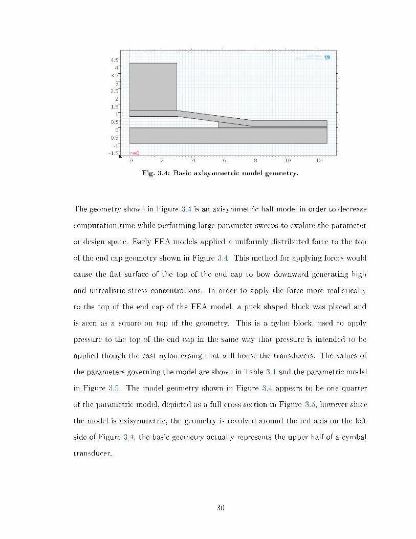
3.4 Basic axisymmetric model geometry. . . . . . . . . . . . . . . . . . . 30
3.5 Parametric cross section model of a Cymbal transducer for FEA purposes. 31
3.6 FEA geometry mesh. . . . . . . . . . . . . . . . . . . . . . . . . . . . 32
3.7 Maximum calculated stress in the stainless steel end cap. . . . . . . 37
3.8 Maximum calculated stress in the piezo disc. . . . . . . . . . . . . . . 37
3.9 Total electric energy produced under compression. . . . . . . . . . . . 37
3.10 Maximum stress in the end cap while varying the ooze depth. . . . . 39
3.11 Max stress in the piezo material while varying ooze depth. . . . . . . 39
3.12 Electrical energy generated as a function of ooze depth. . . . . . . . . 40
3.13 Preload model FEA mesh. . . . . . . . . . . . . . . . . . . . . . . . . 43
3.14 Peak piezo material stress for the range of end cap thicknesses and
preload tensions examined. . . . . . . . . . . . . . . . . . . . . . . . 45
ix

3.15 Peak stress in the epoxy region of the model in a range of and cap
thicknesses and preload tensions tested. . . . . . . . . . . . . . . . . . 45
3.16 Peak stress in the stainless steel end cap region of the model in a range
of and cap thicknesses and preload tensions. . . . . . . . . . . . . . . 46
3.17 Analytic preload model cross section. . . . . . . . . . . . . . . . . . . 47
3.18 Analytic model top view. . . . . . . . . . . . . . . . . . . . . . . . . . 48
3.19 A single twelfth slice of a six slit transducer with a rough mesh for
testing model stability . . . . . . . . . . . . . . . . . . . . . . . . . . 50
3.20 Slit model parametric study results, varying the number of slits. . . . 51
3.21 Maximum end cap stresses in the slit model plotted against end cap
thickness. . . . . . . . . . . . . . . . . . . . . . . . . . . . . . . . . . 52
3.22 Maximum PZT stresses in the slit model plotted against end cap thick-
ness. . . . . . . . . . . . . . . . . . . . . . . . . . . . . . . . . . . . . 52
4.1 Bridge transducer. . . . . . . . . . . . . . . . . . . . . . . . . . . . . 54
4.2 Cymbal end cap male and female dies attached to a die set (center-left)
with bridge dies (right). . . . . . . . . . . . . . . . . . . . . . . . . . 55
4.3 Manual press for operating the die set. . . . . . . . . . . . . . . . . . 55
4.4 Early tested vehicle harvester. . . . . . . . . . . . . . . . . . . . . . 56
4.5 MTS® test setup. . . . . . . . . . . . . . . . . . . . . . . . . . . . . . 57
4.6 Example harvester traces measured during the MTS® tests. . . . . . 58
4.7 Machined cast nylon individual transducer test housing. . . . . . . . 60
x

4.8 Image of a slitted (left) and solid (right) transducers assembled before
wiring and testing. . . . . . . . . . . . . . . . . . . . . . . . . . . . . 61
4.9 The over performing transducer, Slitted Transducer 2. . . . . . . . . 62
4.10 The under performing transducer (Taken apart after the test), Slitted
Transducer 1. . . . . . . . . . . . . . . . . . . . . . . . . . . . . . . . 63
4.11 Traces of tested transducers during 1st test. . . . . . . . . . . . . . . 63
4.12 One of the solid end capped transducers (Solid Transducer 1), taken
apart after the test. . . . . . . . . . . . . . . . . . . . . . . . . . . . . 64
4.13 The other solid end capped transducer (Solid Transducer 2) taken apart
after the test (The PZT material cracked during disassembly). . . . . 65
4.14 The rebuilt transducers from left to right: Slitted Transducer 2, Slitted
transducer 1, Solid traducer. . . . . . . . . . . . . . . . . . . . . . . . 66
4.15 Traces from the epoxy ooze MTS® test. . . . . . . . . . . . . . . . . 66
4.16 Slitted Transducer 1 after testing. The break seems to be caused by
the small patch without epoxy near the left edge of the end cap on the
right. . . . . . . . . . . . . . . . . . . . . . . . . . . . . . . . . . . . . 67
4.17 Slitted Transducer 2 after testing. The failure in this case seems to be
caused by the larger lump of conductive epoxy near the top left of the
left hand end cap. . . . . . . . . . . . . . . . . . . . . . . . . . . . . . 68
4.18 The solid transducer that performed very well and did not fail during
the test despite small conductive epoxy ooze seen on the left end cap. 68
4.19 Six and four slit transducer end caps produced by water jet cutting
compared to the plain versions on the right. . . . . . . . . . . . . . . 69
xi

4.20 Preloaded transducers next to their non-preloaded counterparts (left)
and assembled water cut end cap slitted transducers (right). . . . . . 70
4.21 Trace of the four slit transducer. . . . . . . . . . . . . . . . . . . . . . 70
4.22 The six slitted transducer after testing. . . . . . . . . . . . . . . . . . 71
4.23 Preloaded transducer after 5 KN load. . . . . . . . . . . . . . . . . . 71
4.24 Failure of the preloaded cymbal transducer with 0.017 (0.432 mm)
thick end caps. . . . . . . . . . . . . . . . . . . . . . . . . . . . . . . 72
4.25 Failure of the non-preloaded cymbal transducer with 0.017 (0.432 mm)
thick end caps. . . . . . . . . . . . . . . . . . . . . . . . . . . . . . . 73
4.26 First failure of the non-preloaded, 0.013 (0.330 mm) transducer. . . . 74
4.27 Second failure of the non-preloaded, 0.013 (0.330 mm) transducer. . . 74
4.28 Failure of the preloaded cymbal transducer with 0.013 (0.330 mm)
thick end caps. . . . . . . . . . . . . . . . . . . . . . . . . . . . . . . 75
4.29 The preloaded six slit transducer after testing (left) The same trans-
ducer with the testing pucks removed (right). . . . . . . . . . . . . . 76
4.30 Preloaded six slitted transducer trace. . . . . . . . . . . . . . . . . . . 77
4.31 The solid end capped transducers after the MTS® test (numbered 1-4
from the left). . . . . . . . . . . . . . . . . . . . . . . . . . . . . . . . 78
4.32 Solid transducers after testing with end caps removed (ordered 1-4 from
the left). . . . . . . . . . . . . . . . . . . . . . . . . . . . . . . . . . . 79
4.33 Voltage trace of transducer 1 for a sinusoidal load of 0 - 200 N labeled
V1-0-200 and for a load range of 0 - 250 N labeled V1-0-250. . . . 81
xii

4.34 Fujilm Prescale sample pack. . . . . . . . . . . . . . . . . . . . . . 82
4.35 Tekscan® FlexiForce® A201 force sensor. . . . . . . . . . . . . . . . 83
4.36 Omega® KFH-03-120-C1-11L1M2R strain gauge. . . . . . . . . . . . 83
4.37 Omega® strain gauge mounted on a preloaded transducer. . . . . . . 84
4.38 Bridge circuit used to measure preload stress. . . . . . . . . . . . . . 85
4.39 A preloaded and slitted transducer set to the correct preload. . . . . . 87
4.40 Barco mini speed hump section. . . . . . . . . . . . . . . . . . . . . . 88
4.41 Power harvesting module design for accommodating preloaded trans-
ducers. . . . . . . . . . . . . . . . . . . . . . . . . . . . . . . . . . . . 89
4.42 Power harvesting module design for standard cymbal transducers. . . 89
4.43 Slitted end caps before and after stamping. . . . . . . . . . . . . . . . 90
4.44 Preloaded transducers being epoxied (left) and the hardened transduc-
ers (right). . . . . . . . . . . . . . . . . . . . . . . . . . . . . . . . . . 90
4.45 Preloaded transducers being paired up and electrically connected (left)
and the nished preloaded transducers (right). . . . . . . . . . . . . . 91
4.46 Preloaded transducer housing after machining with inserted transducers. 92
4.47 Under performing slitted transducer. . . . . . . . . . . . . . . . . . . 93
4.48 Machined non preloaded transducer housing module sitting in the speed
bump. . . . . . . . . . . . . . . . . . . . . . . . . . . . . . . . . . . . 94
4.49 Fully assembled non preloaded harvester. . . . . . . . . . . . . . . . . 94
xiii

4.50 Harvesters inserted into speed bump. . . . . . . . . . . . . . . . . . . 95
4.51 Vehicle test setup. . . . . . . . . . . . . . . . . . . . . . . . . . . . . . 96
4.52 Trial 1 traces. . . . . . . . . . . . . . . . . . . . . . . . . . . . . . . . 99
4.53 Trial 2 traces showing backward driving on the left, and forward driving
on the right. . . . . . . . . . . . . . . . . . . . . . . . . . . . . . . . 100
4.54 Trial 3 traces. . . . . . . . . . . . . . . . . . . . . . . . . . . . . . . . 101
4.55 Trial 7 traces showing voltage spikes corresponding to the heavier front,
and lighter rear tire loads. . . . . . . . . . . . . . . . . . . . . . . . . 102
4.56 Summary of all the peak voltages of the August vehicle testing. . . . 102
4.57 Vehicle speed test setup. . . . . . . . . . . . . . . . . . . . . . . . . . 103
4.58 Peak open circuit voltages vs speed. . . . . . . . . . . . . . . . . . . 104
4.59 Traces from the experimental transducers with foam padding removed. 105
4.60 Peak open circuit voltages vs speed with foam padding removed. . . . 106
4.61 Waterproofed harvesting pads. . . . . . . . . . . . . . . . . . . . . . 107
4.62 Reduced preload traces. . . . . . . . . . . . . . . . . . . . . . . . . . 108
4.63 Short term degradation test. . . . . . . . . . . . . . . . . . . . . . . . 109
4.64 Peak voltages plotted against speed for the reduced preload tests. . . 109
4.65 Damaged transducer traces. . . . . . . . . . . . . . . . . . . . . . . . 111
4.66 Damaged transducer in a pair. . . . . . . . . . . . . . . . . . . . . . 111
xiv

4.67 Damaged piezo disc from Figure 4.66. . . . . . . . . . . . . . . . . . . 112
4.68 The second damaged transducer disassembled. . . . . . . . . . . . . . 112
4.69 The most heavily damaged piezo unit examined. . . . . . . . . . . . . 112
4.70 Improved harvesting pad housing design. . . . . . . . . . . . . . . . . 114
4.71 Transducers at various stages of assembly. . . . . . . . . . . . . . . . 114
4.72 A single harvesting pad wired and sealed with electrical tape. . . . . 115
4.73 Speed bump with truss connector plates used to attach the wooden
spacers. . . . . . . . . . . . . . . . . . . . . . . . . . . . . . . . . . . 116
4.74 Harvesting pads on top of and placed in the speed bump. . . . . . . . 116
4.75 Full scale harvester test setup. . . . . . . . . . . . . . . . . . . . . . . 117
4.76 Initial compression with only harvesting pad 2. . . . . . . . . . . . . . 118
4.77 Schematic for a voltage divider used to allow measurement of higher
voltages. . . . . . . . . . . . . . . . . . . . . . . . . . . . . . . . . . . 118
4.78 Calculated full scale traces from initial front wheel loading. . . . . . . 119
4.79 All seven, 20 lb weights placed in the rear of the test vehicle. . . . . 120
4.80 Calculated voltage traces for rear wheel loading scenarios. . . . . . . 121
4.81 Calculated peak voltages from all harvesting pads plotted against the
added mass for rear wheel loading scenarios. . . . . . . . . . . . . . 121
4.82 Vehicle speed vs average peak harvesting pad voltage. . . . . . . . . . 122
xv

Nomenclature
Abbreviations
AADT Annual Average Daily Trac
APC American Piezo Ceramics International Ltd
CNC Computer Numeric Control
DC Direct Current
DIP Dual Inline Package
FEA Finite Element Analysis
LED Light Emitting Diode
MATLAB MATrix LABoratory
MEMS Micro Electro Mechanical Systems
MFC Micro Fiber Composites
PCB Printed Circuit Board
PVDF Polyvinylidene uoride, a piezoelectric polymer
PZT Lead Zirconate Titanate
SONAR SOund Navigation And Ranging
THUNDER THin layer UNimorph ferroelectric DrivER and sensor
Mathematical Symbols
ε Permittivity tensor . . . . . . . . . . . . . . . . . . . . . . . . . . . . . . . . . . . . . . . . . . [F/m]
xvi

εT11 Permittivity perpendicular to polarization direction . . . . . . . . . . [F/m]
εT33 Permittivity parallel to polarization direction . . . . . . . . . . . . . . . . [F/m]
cE Stiness under a constant electric eld . . . . . . . . . . . . . . . . . . . . . . . . . [Pa]
Cs Capacitance of a piezo disc . . . . . . . . . . . . . . . . . . . . . . . . . . . . . . . . . . . . . [F]
D Surface charge density . . . . . . . . . . . . . . . . . . . . . . . . . . . . . . . . . . . . . . [C/m2]
d Piezoelectric charge constant . . . . . . . . . . . . . . . . . . . . . . . . . . . . . . . . [C/N]
dxy Piezoelectric charge constant with polarization direction x and strain
in direction y . . . . . . . . . . . . . . . . . . . . . . . . . . . . . . . . . . . . . . . . . . . . . . . . [C/N]
E Electric eld strength . . . . . . . . . . . . . . . . . . . . . . . . . . . . . . . . . . . . . . . [V/m]
e A tensor that relates stress to surface charge density . . . . . . . . [C/m2]
F An applied force . . . . . . . . . . . . . . . . . . . . . . . . . . . . . . . . . . . . . . . . . . . . . . . . [N]
Fnorm Normal force . . . . . . . . . . . . . . . . . . . . . . . . . . . . . . . . . . . . . . . . . . . . . . . . . . . [N]
Fr Total radial compressive force . . . . . . . . . . . . . . . . . . . . . . . . . . . . . . . . . . [N]
g Piezoelectric voltage constant . . . . . . . . . . . . . . . . . . . . . . . . . . . . [V ·m/N]
gxy Piezoelectric charge constant with polarization direction x and strain
in direction y . . . . . . . . . . . . . . . . . . . . . . . . . . . . . . . . . . . . . . . . . . . . . [V ·m/N]
GF Gauge factor
h Electric eld strength per unit strain . . . . . . . . . . . . . . . . . . . . . . . . [N/C]
kp Electromechanical coupling factor, used for thin discs, with electric
eld in direction 3 and radial vibrations in directions 1 and 2 . . . [%]
xvii

k2p Electromechanical coupling factor for a thin piezoelectric disc being
stressed at static or low frequencies
kt Electromechanical coupling factor used for thin discs . . . . . . . . . . . [%]
kxy Electromechanical coupling factor with electric eld in direction x and
vibrations in direction y . . . . . . . . . . . . . . . . . . . . . . . . . . . . . . . . . . . . . . . . [%]
KTxy Relative dielectric constant, at a constant force in direction y, with
polarization in direction x
N Number of radial wedges
Q Generated charge . . . . . . . . . . . . . . . . . . . . . . . . . . . . . . . . . . . . . . . . . . . . . . . [C]
s Elastic compliance . . . . . . . . . . . . . . . . . . . . . . . . . . . . . . . . . . . . . . . . . . [m2/N]
sE Compliance under a constant electric eld . . . . . . . . . . . . . . . . . . [m2/N]
sE11 Elastic compliance perpendicular to polarization direction, connected
in short circuit . . . . . . . . . . . . . . . . . . . . . . . . . . . . . . . . . . . . . . . . . . . . . [m2/N]
sD33 Elastic compliance parallel to polarization direction, connected in open
circuit . . . . . . . . . . . . . . . . . . . . . . . . . . . . . . . . . . . . . . . . . . . . . . . . . . . . . . [m2/N]
u Displacement . . . . . . . . . . . . . . . . . . . . . . . . . . . . . . . . . . . . . . . . . . . . . . . . . . . [m]
V Voltage . . . . . . . . . . . . . . . . . . . . . . . . . . . . . . . . . . . . . . . . . . . . . . . . . . . . . . . . . [V]
Vc Static voltage of a piezoelectric ring under compression . . . . . . . . . [V]
Vrt Static voltage of a piezoelectric disc under radial tension . . . . . . . . [V]
W Work . . . . . . . . . . . . . . . . . . . . . . . . . . . . . . . . . . . . . . . . . . . . . . . . . . . . . . . . . . . [J]
X Mechanical strain . . . . . . . . . . . . . . . . . . . . . . . . . . . . . . . . . . . . . . . . . . . . . . [%]
xviii

x Mechanical stress . . . . . . . . . . . . . . . . . . . . . . . . . . . . . . . . . . . . . . . . . . . . . . [Pa]
Yxy Young's modulus . . . . . . . . . . . . . . . . . . . . . . . . . . . . . . . . . . . . . . . . . . . . . . [Pa]
ID Inside diameter parameter . . . . . . . . . . . . . . . . . . . . . . . . . . . . . . . . . . . . . . [m]
OD Outside diameter parameter . . . . . . . . . . . . . . . . . . . . . . . . . . . . . . . . . . . . [m]
t Thickness parameter . . . . . . . . . . . . . . . . . . . . . . . . . . . . . . . . . . . . . . . . . . . [m]
xix

1 Introduction
This work covers the motivation, background, design, and testing of a piezoceramic
based power harvesting system designed to harvest power from vehicles. The nal
goal of this project is to build working prototypes of a roadway power harvesting
system to be implemented in either speed bumps, or in the road surface itself. Using
the aforementioned piezoelectric technology, the speed bump would be able to store
and power a variety of applications through on board power harvesting circuitry and
power conditioning circuitry to deliver the power at a variety of voltages. The number
of speed bumps or harvesting pads, the number of power harvesting transducers per
pad, and the electrical storage capacity would be determined by the power demanded
by a specic application.
1.1 Motivation
As more people become aware of the eects of global warming, there is greater com-
mercial pressure to develop sustainable energy technologies. One area that has at-
tracted some attention is roadway power harvesting using piezoelectric materials [1].
Power harvesting is not only attractive for its use of so called green energy but is also
useful for replacing batteries as power sources where applicable with the added benet
of not needing replacement [2]. Finally a very large proportion of energy that is used
by vehicles is given o in the form of waste heat from braking and road deformation
[3, 4]. This energy can be recovered for other purposes by placing roadway power
1

harvesters on roadways, in particular areas of vehicle deceleration or where power is
needed.
In addition to the stated goals, automated speed measurement is also explored for
harvesting pads with two or more piezoelectric harvesting arrays. Although not part
of the objectives, speed measurement would make an interesting additional feature
to any future product that may come from this research.
Pavegen is a company based in the United Kingdom, striving to produce an energy
harvester that is economically viable on a large scale and is producing a series of pedes-
trian footstep harvesting pads that use a mechanism to apply stress to piezoelectric
materials [5]. Another Israeli company Innowattech is also developing piezoelectric
power harvesters using simple rods of PZT [6] for applications in roadway power
harvesting, railway power harvesting, and airport runway power harvesting [7, 8].
Currently there are few commercial roadway power harvesting technologies in exis-
tence, and those that do exist have not been implemented on a large scale. Because
of this, BW Services and MITACS funded this research to produce a roadway power
harvesting device.
1.2 Background
This section provides background information on piezoelectric materials, power har-
vesting projects and applications as well as research performed in this area. Funda-
mental governing equations for piezoelectric materials are also covered.
1.2.1 Piezoelectric applications
Piezoelectric materials are widely used today in a variety of applications. From pres-
sure sensors, accelerometers, microphones, SONAR and ultrasound systems all the
2

way to gas lighters, buzzers and clocks, piezoelectric materials are used in many
aspects of daily life [9, 10, 11, 12, 13, 14, 15, 16]. Piezoelectric energy harvesting
has been applied to many situations that involve vibrations and where it is di-
cult to attach xed power cables such as ocean buoys, knapsack straps, and shoes
[17, 18, 19, 20, 21].
Due to its uniform crystal nature, Piezoelectric materials allowMicro-Electro-Mechanical
Systems (MEMS) such as accelerometers and clock oscillators to be made cheaply and
in very small packages. Piezoelectric accelerometers work by attaching small masses
through piezoelectric pads to a base xed to the sensor body. When the sensor body
accelerates, the small internal mass will put the piezo element under stress, gener-
ating a proportional voltage to the acceleration. Quartz crystal clocks use specic
congurations of quartz crystals, usually shaped as thin plates or tuning forks, and
include them as a component of an electronic oscillator. The quartz crystals help
produce very stable oscillation frequencies and thereby keep accurate time. Piezo-
electric SONAR and ultrasound systems take advantage of the inverse piezoelectric
eect, and are able to produce powerful sound waves at much higher frequencies than
conventional speakers by replacing the coil actuator with a piezoelectric one. High
voltages can be reached when striking piezo materials, paving way for the existence of
reliable and small gas lighters without the need for batteries or other external power
sources. Piezoelectric gas lighters use a mechanism to store energy in a spring, which
is compressed by a user, until it is fully compressed. This causes the spring to release,
striking a mass into the piezoelectric element which in turn generates a high voltage
and a visible spark. Often pressure sensors will use thin lm piezoelectric materials
spread over a small hole exposed to an external pressure. This method of pressure
sensing allows for large pressures to be measured at high accuracy and even allows
for absolute pressure measurement.
3

1.2.2 Vehicle energy harvesting
Apart from piezoelectric based roadway power harvesting, research has been put into
power recovery from vehicles using permanent magnet linear generators as discussed
and demonstrated in [22] and hydraulic systems which are demonstrated in [3]. How-
ever most research appears to employ piezoelectric materials for power harvesting due
to the lack of moving parts required and compact sizing, allowing for easier design,
installation, and maintenance of power harvesting roads and pads [1, 4, 23, 24, 25, 26]
1.2.3 Piezoelectric materials
Piezoelectric materials generate an electric potential by way of electric eld generation
when stressed, called the piezoelectric eect. The inverse piezoelectric eect is also
possible by way of inducing a strain in the material after an electric potential is
applied.
There are a wide variety of piezoelectric materials, all well suited to various appli-
cations [2, 9, 27]. Natural and synthetic quartz crystals, a crystalline form of silicon
dioxide, are an example of a non ferroelectric piezoelectric material. Generally non
ferroelectric materials exhibit poorer piezoelectric properties but are still useful for
applications as sensors such as pressure, gyroscopic, and microphone sensors. The
largest use of quartz is as a resonator used for timing circuits in clocks, computer
processors, and transmitter/receivers, to name a few.
Piezoelectric polymers are another family of piezoelectric materials geared toward
their own set of applications. These polymers can be manufactured at lower tem-
peratures and oer high exibility and mechanical stability. With poor piezoelectric
properties, these polymers are poorly suited for actuators but can work well as sen-
sors. Among the few known piezoelectric polymers, Polyvinylidene Fluoride (PVDF)
4

is one of the most widely used. Applications include vibration dampening actuators
and articial muscles. PVDF has even been experimentally used in shoes [2, 21]. Lead
(Pb) Zirconate Titanate (PZT) is a ceramic and ferroelectric piezoelectric material
which has excellent piezoelectric properties sometimes hundreds of times higher than
quartz [28]. It is commonly used in transducers and actuators because of its piezo-
electric and mechanical properties. PZT is a synthetic crystal with chemical formula
PbZr(Ti)O3 in a perovskite structure. For thin lms, PZT can be manufactured by
chemical vapor deposition however for transducer and actuator applications where
thicker solids are desired another technique is used. Powder components of the PZT
crystal are combined with each other and a polymer binder in a mold and compressed
under high heat. After the molding process is complete, the PZT components are
red in order to nalize the sintering process. Finally a large electric eld is applied
to set the polarity direction while the material is held above its Curie temperature.
Without the polarization process, the PZT crystals would produce no net electric eld
when the material is strained. The specic properties of a PZT material can be mod-
ied by changing the zirconia to titania ratio of the precursor powders [28]. Because
of these benets, PZT is the chosen material for the piezoelectric power harvesting
project presented here.
PZT is popular because of its piezoelectric properties, however being a ceramic causes
that material to be brittle and therefore unsuited to many applications. In order to
get the desired material properties, piezoelectric composites have been created which
are called Micro Fiber Composites (MFC). Three main piezo composites, typically
using PZT and a binding polymer such as epoxy, exist: 0-3, 1-3, and 3-3. The rst
digit represents the number of directions that the piezoelectric material is connected
in and the second represents the directions in which a binding polymer is connected
in. 0-3 composites are formed by evenly dispersing powdered PZT within a polymer.
Composites composed of PZT laments suspended in a polymer are classed as 1-3
5

and nally larger chunks and networks of PZT in suspension is referred to as a 3-
3 composite. Even though these composites have improved strength characteristics
compared to ceramic PZT components, the reduced amount of piezoelectric material
also reduces the overall charge available to be harvested in compression. For this
reason these materials were not used in this research project.
1.2.4 Piezoelectric notation
Piezoelectric materials have the ability to convert mechanical energy into electric
charge or to convert electric charge into mechanical energy. The process of convert-
ing mechanical into electrical energy is called the piezoelectric eect [2, 11, 20, 29].
Conversely, the process of converting electrical into mechanical energy is called the
inverse or converse piezoelectric eect. Because piezoelectric materials are anisotropic
a common vector notation seen in literature and industrial purposes is Voigt notation
[11, 30]. This notation replaces standard right hand coordinate directions x, y, z and
rotations about x, y, and z with the digits 1 - 6. Piezoelectric materials that are
deformed in dierent directions will behave dierently because of their anisotropy.
Piezoelectric generator modes are the term used to refer to piezoelectric loading di-
rections and their calculations. Figure 1.1 demonstrates two common modes, mode
33 on the left, and mode 31 on the right. The rst digit refers to the poling direction
represented in Figure 1.1 by the vector marked P. This is the direction that an electric
eld was applied when the material was being manufactured and is conventionally
aligned with the Z axis. The second digit refers to the loading direction which an
applied force is aligned to. Most piezoelectric materials that are symmetric about the
X-Z plane will have properties that are equal in 31 mode and 32 mode.
6

Fig. 1.1: Piezoelectric generator modes: mode 33 (left) and mode 31 (right).
The following equations model the behavior of piezoelectric materials [28]. Surface
charge density and electric eld are proportional to mechanical strain as described in
Equations 1.1 and 1.2.
D = dx (1.1)
E = gx (1.2)
Where D is the surface charge density, E is the electric eld, and x is the input
mechanical stress. Here d(CN
)and g
(V ·mN
)are piezoelectric constants unique for
every piezoelectric material and often refered to as the piezoelectric charge and voltage
constants respectively. The stress, x, is a second order tensor of the form:
x =
x11 x12 x13
x22 x23
sym x33
. (1.3)
7

Since x has six independent values, it is often rewritten in Voigt notation as a vector
[2, 9, 30, 31]:
x =
x11
x22
x33
x23
x13
x12
=
x1
x2
x3
x4
x5
x6
. (1.4)
Similarly D is a three component vector:
D =
D1
D2
D3
. (1.5)
Equation 1.1 can then be rewritten as:
D1
D2
D3
=
d11 d12 d13 d14 d15 d16
d21 d22 d23 d24 d25 d26
d31 d32 d33 d34 d35 d36
x1
x2
x3
x4
x5
x6
. (1.6)
We can see that the piezoelectric constant d can be represented as a 3×6 matrix.
Strain X is also a second order tensor like the stress tensor x and can be written
8

similarly to x in Equations 1.3 and 1.4. X can then be written in terms of x by the
elastic compliance constant s shown in Equation 1.7.
X1
X2
X3
X4
X5
X6
=
s11 s12 s13 s14 s15 s16
s21 s22 s23 s24 s25 s26
s31 s32 s33 s34 s35 s36
s41 s42 s43 s44 s45 s46
s51 s52 s53 s54 s55 s56
s61 s62 s63 s64 s65 s66
x1
x2
x3
x4
x5
x6
(1.7)
The surface charge density and electric eld can be related through the permittivity
tensor dened as:
D1
D2
D3
=
ε11 ε12 ε13
ε21 ε22 ε23
ε31 ε32 ε33
E1
E2
E3
. (1.8)
Because the piezoelectric material, PZT, being used is in a crystalline structure and
is poled in such a way to make it symmetric about the single poled axis (convention-
ally assumed to be the z-axis or direction 3) the Equations 1.6, 1.7, and1.8 can be
simplied and rewritten using Equations 1.9, 1.10, and 1.11.
[d] =
0 0 0 0 d15 0
0 0 0 d15 0 0
d31 d31 d33 0 0 0
, (1.9)
where d15 = d51 and d13 = d31 because of symmetry. s becomes:
9

[s] =
s11 s12 s13 0 0 0
s12 s11 s13 0 0 0
s13 s13 s33 0 0 0
0 0 0 s44 0 0
0 0 0 0 s44 0
0 0 0 0 0 2 (s11 − s12)
, (1.10)
where s11 = s22, s12 = s21, s13 = s31, s44 = s55, and s66 = 2 (s11 − s12). And nally ε
becomes:
[ε] =
ε1 0 0
0 ε2 0
0 0 ε3
, (1.11)
where ε1 = ε2. The governing equations for the piezoelectric eect then take on two
forms based on boundary conditions. In the case where the piezoelectric material is
free to expand and contract along with changing electric eld the governing equation
becomes:
D = dx+ εE. (1.12)
In the case where the piezoelectric material is clamped, the equation becomes:
D = eX + εE, (1.13)
where e is the tensor that relates the stress to the surface charge density.
10

The indirect piezoelectric eect can also be described using the following equations.
In the case were the piezoelectric material is under a constant electric eld, which
corresponds to the material in a short circuit, the governing equation becomes:
X = sEx+ dE, (1.14)
x = cEX − eE, (1.15)
where sE and cE are the compliance and stiness under a constant electric eld.
In the other case, where the piezoelectric material is in a constant charge density,
corresponding to the material connected in open circuit. The equations then become:
X = sDx+ gD (1.16)
x = cDX − hD. (1.17)
where h is the electric eld strength per unit strain.
1.2.5 Piezoelectric material properties
Piezoelectric materials are anisotropic and so the notation used allows subscripts to
dene the poling and loading directions that the specic property applies in.
11

Table 1.1: Piezoelectric properties nomenclature
Symbol Description
dxy
Piezoelectric charge constant with polarization direction x and strainin direction y
gxy
Piezoelectric voltage constant with electric eld in direction x andstrain in direction y
εT11
Permittivity perpendicular to polarization direction
εT33
Permittivity parallel to polarization direction
sE11
Elastic compliance perpendicular to polarization direction, connectedin short circuit
sD33
Elastic compliance parallel to polarization direction, connected inopen circuit
kxy
Electromechanical coupling factor with electric eld in direction x andvibrations in direction y
kt
Electromechanical coupling factor used for thin discs
kp
Electromechanical coupling factor, used for thin discs, with electriceld in direction 3 and radial vibrations in directions 1 & 2
QGenerated charge
KTxy
Relative dielectric constant, at a constant force in direction y, withpolarization in direction x
The piezoelectric properties in Table 1.1 can be related to each other and other
physical properties using the following equations [2, 11, 28]. Equation 1.18 relates
the elastic compliance to the young's modulus of the material.
sxy =1
Yxy(1.18)
k2p =
2d231
((sE11 + sE12) εT33)(1.19)
12

Equation 1.19 describes the electromechanical coupling factor for a thin piezoelectric
disc being stressed at static or low frequencies.
gxy =dxyεTxy
(1.20)
V =gxyFt
A(1.21)
Equation 1.20 relates the piezoelectric voltage constant to the piezo charge constant.
While Equation 1.21 returns the static voltage of a piezo material under load in the y
direction, and polarization in the x direction. In this equation, F is an applied force
to the piezo unit, t is the thickness along which the force is being applied, and A is
the cross sectional area perpendicular to the direction of applied force. The forces
applied to the piezoelectric disc in any cymbal style transducer are a combination of
compression of the outer ring, and a radial tension, both forces being applied by the
end cap. These two eects can be superimposed on each other [9, 32]. Equation 1.22
denes the capacitance of a piezo disc, where h is the thickness of the disc, and r is
the radius.
Cs =KT
33ε0πr2
h(1.22)
Vrt =g31Fr2πr
(1.23)
Vc =4g33F3h
π (OD2 − ID2)(1.24)
13

where OD and ID are the outside and inside diameters dening the ring shaped
region of the piezoelectric disc being compressed. Equations 1.23 and 1.24 are the
static voltages of a piezoelectric disc under radial tension, and compressed piezo ring
respectively. By using equations 1.22, 1.23, and 1.24, the total energy harvested
from a given force can be estimated. Conversely it may be possible to use the above
equations to estimate vehicle weight and transducer performance separately.
1.3 Thesis overview
Chapter 2: Power harvesting electronics
This chapter covers information on various piezoelectric power harvesting circuitry
topologies as well as feasibility calculations using the circuitry concepts to produce
an estimate of the amount of power that could be generated from a set number of
harvesters. This estimated power is compared to a potential application to conclude
that the estimated energy generation amount is sucient for the potential application.
Chapter 3: Transducer design
This chapter focuses on the physical design of transducers, giving a background to
other transducer designs made along with their applications. A novel variant of the
Cymbal transducer designed for vehicle power harvesting is also introduced along with
Finite Element Analysis (FEA) models. FEA is used to examine existing designs and
to assist in nding improved design parameters for improved performance.
Chapter 4: Implementation and testing
14

This chapter documents the generations of prototyped transducers and what was
learned from them. It also discusses the manufacturing processes and implementa-
tion of the transducers into nylon housings to be implanted into rubber speed bumps.
Results from both MTS hydraulic testing apparatus and vehicle tests are also pre-
sented here.
Chapter 5: Conclusion
Finally this chapter summaries the conclusions and accomplishments that this study
found along with promising avenues for improvements and future work.
15

2 Power harvesting electronics
This section covers various methods for piezoelectric charge collection in order to
store and deliver the harvested power to lower voltage, higher current applications.
2.1 Brief history of harvesting circuitry
As Piezoelectric materials become stressed by an external load, an electric eld is
generated by the material. Often, fabricated piezoceramic solids, such as PZT, will
have two sides coated in a thin conductive lm. These conductive lm panels behave
like a capacitor allowing the generated electric eld to draw in or push out electrons
from the conductive contact areas. This ow of charge is the source of electrical
energy to be harvested or used by circuitry or an electrical load.
The simplest way of utilizing piezoelectric power is by simply connecting the two con-
tact terminals of a piezoelectric material to an electrical load. Many papers focusing
on transducer design will report voltages attained while attaching a simple resistive
load to a piezo transducer [2, 19, 25, 33, 34]. This method for harvesting power by
direct connection to a load is the least ecient method. This method also generates
inverting and often high voltages and low currents which make them dicult to adapt
to lower voltage and higher direct current loads such as LED lighting or low power
sensors [35].
A simple solution to the above problems is by rectifying the piezo harvesters output,
adding a storage capacitor, and then using a DC - DC step down converter to produce
the desired voltage and current for a specic application. Typically the DC - DC
converter chosen is a buck converter. Modeling the piezoelectric material subjected
to strain can be done by representing the material as a current source with an internal
16

capacitance caused by the electrodes [35]. Because of this, it is benecial to allow the
piezo material to reach a higher voltage and then step the voltage down.
More advanced harvesting circuits tend to improve power harvested by inverting or
charging the internal capacitance of a harvester using an inductor [2, 33, 34, 35, 36, 37].
One way to grasp the reasoning behind inverting or pre-charging the internal piezo
capacitance is by examining the work that the load force must do in order to allow
the full compression of a piezoceramic or piezoceramic device. The total work done
by an external force is shown in Equation 2.1.
W = Fnorm · d (2.1)
Where W is the work done by an external force, Fnorm which is the normal force
resisting the external force, and d is the displacement of the compressed piezo unit
under the external load. The total work can then be increased by increasing the nor-
mal force required to compress a piezoelectric transducer, assuming that the external
force is sucient to compress the transducer to its maximum allowed displacement.
The stiness of any piezoelectric material is determined by the superposition of its
mechanical stiness along with the electric eld within the material due to the inverse
piezoelectric eect [9]. Thus a circuit that inverts or applies an initial charge to a
piezo material just before it is loaded will allow the external load to generate more
work, assuming that it compresses the piezoelectric transducer a xed amount, and
therefor increase the amount of energy available for harvesting.
These circuits are referred to as synchronous circuits and are similar to the one that
will be used with this project.
17

2.2 The circuit model
The harvesting circuit being used for this project synchronizes the discharge of the
piezoelectric materials with their peak voltage. As the piezoelectric material ap-
proaches its peak voltage caused by its peak strain, a peak detection circuit triggers
the harvesting circuit to drain the piezoelectric capacitor into a storage capacitor.
This means that the energy gathered can be approximated by Equation 2.2 where V
is the peak voltage of the piezoelectric material. This equation ignores losses in the
circuitry, dissipation from measurement equipment, and the voltage of the storage
capacitor.
E =1
2CV 2 (2.2)
A variety of possible piezoceramic materials exist for use in power harvesting applica-
tions. American Piezo Ceramics (APC) is a company that provides custom fabricated
piezoelectric materials as well as testing samples. Their materials were considered be-
cause of the ease of purchasing samples from them which suited the initial testing
phases of the project. A variety of APC materials are shown in Table 2.1.
Table 2.1: APC materials and their d · g values.
Material (navy type equivalent) d31 · g31 d33 · g33 d15 · g15
840 (Navy I) 1.38 7.69 18.2841 1.14 7.65 15.8
850 (Navy II) 2.17 9.92 21.2855 (Navy VI) 2.48 13.2 19.4880 (Navy III) 0.950 5.38 9.24
842 - 7.89 -844 - 7.35 -851 - 9.92 -881 - 5.87 -
Units in (×10−12 m s2
kg)
18

APC International Ltd 855 material was chosen for its high d33 ·g33 and d31 ·g31 values,
which represent one of the more desirable metrics for a PZT harvesting transducer
[20, 28, 38]. Several PZT samples made of APC 855 were purchased with readily
available dimensions. The sample discs had a diameter of 25.4 mm and a thickness
of 2 mm. The capacitance can be estimated for the disc using Equation 1.22:
Cs =3, 300 (8.85× 10⁻¹²) π0.01272
0.002= 6.73 nF.
A Tektronix DMM4050 multimeter was used to measure the capacitance of the PZT
disc. The measured capacitance from the probes was 0.035 nF and the measured
capacitance of a piezo unit was 7.94 nF. Equivalently then, the capacitance of the
piezo unit should be the dierence of these, being 7.91 nF. The measured value is
about 18% larger than the calculated value and is probably due to variations between
the materials actual properties, and the reported properties. To represent the piezo-
electric material more accurately, the measured value will be used in calculations.
We are using a synchronous circuit that will empty the transducer voltage into a
storage capacitor when the transducer reaches its peak voltage. Because the charge
is transferred from the piezoelectric power bank into a storage capacitor, not all the
charge can be transferred, and so the energy transferred should be:
Etransfer = Etotal − EleftOver,
Etransfer =1
2CpiezoV
2piezo −
1
2CpiezoV
2storage, (2.3)
19
where Etransfer is the total energy being transferred over from a piezo transducer,
Etotal is the total energy stored in the transducer at its peak voltage, and nally
EleftOver is the leftover energy stored in the transducer after the synchronous circuit
has discharged Etransfer into the storage capacitor bank assuming that the storage
capacitance is much larger than the capacitance of the transducer. The size of storage
capacitor would vary from power harvesting application to power harvesting appli-
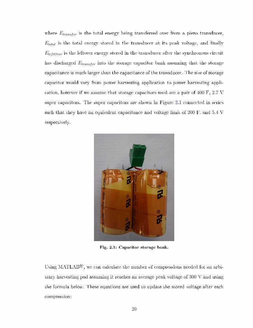
cation, however if we assume that storage capacitors used are a pair of 400 F, 2.7 V
super capacitors. The super capacitors are shown in Figure 2.1 connected in series
such that they have an equivalent capacitance and voltage limit of 200 F, and 5.4 V
respectively.
Fig. 2.1: Capacitor storage bank.
Using MATLAB®, we can calculate the number of compressions needed for an arbi-
trary harvesting pad assuming it reaches an average peak voltage of 300 V and using
the formula below. These equations are used to update the stored voltage after each
compression:
20

VstorageNew =
√2
Cstorage(Etransfer + Estorage)
VstorageNew =
√2
Cstorage
(1
2CpiezoV 2
piezo −1
2CpiezoV 2
storageOld +1
2CstorageV 2
storageOld
)
VstorageNew =
√Cpiezo
(V 2piezo − V 2
storageOld
)+ CstorageV 2
storageOld
Cstorage
Iterating the above equations in MATLAB®, the program calculates the results shown
in Table 2.2. Note that the calculation iteratively added optimal amounts of energy
from the piezo units until the goal voltage was met or exceeded. As such the calculated
number of compressions shown in Table 2.2 are rounded up to the nearest whole
number of compressions. The circuit that was used is allowed to store no more than
5 volts, and produces variable voltage power for a given load.
Table 2.2: Calculated compressions needed to charge the 200 F capacitor pack
Storage voltage increase 2 harvesting pads(number of
compressions)
8 harvesting pads(number of
compressions)
0− 5 V 175, 611 43, 9034− 5 V 63, 226 15, 8070− 4 V 112, 386 28, 097
The 0−5 V trial indicates the fully discharged module being charged to maximum op-
erating voltage, 4−5 V represents the harvesting module charging between minimum
and maximum operating voltages and is the intended continuous mode of operation,
and 0− 4 V represents the charging to the minimum operating voltage. This system
can be scaled up linearly to provide more power by simply adding more harvesting
pads or speed bumps.
21

A moderately busy o ramp with 150,000 Annual Average Daily Trac (AADT)
which is common for o ramps in Canadian cities [39], would produce 300,000 com-
pressions (front and rear tire each compressing the harvesting units once) of a smooth
harvesting pad. The optimal total energy generated in a day by eight harvesting pads
can then be calculated as:
(300, 000 compressions
day
15, 807 compressions4−5 V
)1
2(200 F)
((5 V)2 − (4 V)2) = 17, 081
J
day. (2.4)
The average power output for the harvesting pads then becomes:
(17, 081
J
day
)(1
24
day
h
)(1
60
h
min
)(1
60
min
s
)= 0.1977 W (2.5)
MicroStrain® produces a product called EH-Link® [40]. This is a wireless node,
which can connect to a variety of sensors and transmit their measurements in ad-
dition to measurements from its on board accelerometer, temperature and humidity
sensors. The sensor node is designed to run o of ambient energy sources including
piezoelectric power sources. Using all internal sensors, as well as all external sensor
options and operating at the maximum sample rate of 256 Hz the EH-Link® will
consume 18.5325 mW. Choosing lower sampling rates, and using fewer sensors can
drastically reduce the power requirements if they are not needed. Ideally then, 8
harvesting pads could power 0.1977 W0.0185325 W
= 10.67 units or ~1.333 sensor nodes at full
output per harvesting pad. In reality ineciencies will reduce this number, however
this estimate certainly indicates the feasibility of the project.
22

3 Transducer design
This section introduces the design and modeling of the transducer to be used. First
the mathematics behind piezoceramic modeling are covered so that one has an un-
derstanding of what the commercial Finite Element Analysis (FEA) software used
is doing when calculating solutions. Analytical equations are then introduced and
used for estimation purposes of the amount of power that could be harvested by the
harvesting circuitry used, and nally the FEA process is covered in order to justify
design decisions made.
3.1 Transducer designs
There are a variety of transducer designs, piezoelectric devices that convert mechani-
cal work into electricity [38]. In general, dierent transducers are designed for dierent
loading and displacement scenarios. The simplest form of transducer, called the mul-
tilayer transducer, gets its name from its composition simply being several layers of
thin PZT plates. The advantage of the multilayer transducer is that it will produce a
lower voltage and a higher current when compared to a solid block of PZT, however
it will have a similarly high stiness which limits its power harvesting applications to
those that apply very large forces. A more advanced transducer design for power har-
vesting applications is the THUNDER (THin layer UNimorph ferroelectric DrivER
and sensor) transducer which has been implemented in shoe power harvesters [18, 38].
The THUNDER transducer is composed of a curved sheet of PZT laminated between
a thin curved aluminum sheet and a curved stainless steel sheet shown in Figure 3.1.
Although the THUNDER exhibits good eciency and power recovery capabilities,
its very low stiness would be inappropriate for the high stresses expected with the
wheel load of a vehicle.
23
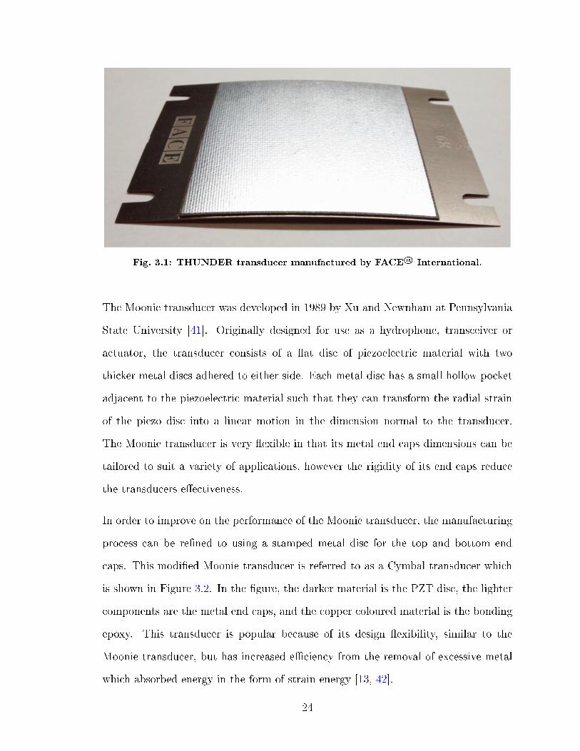
Fig. 3.1: THUNDER transducer manufactured by FACE® International.
The Moonie transducer was developed in 1989 by Xu and Newnham at Pennsylvania
State University [41]. Originally designed for use as a hydrophone, transceiver or
actuator, the transducer consists of a at disc of piezoelectric material with two
thicker metal discs adhered to either side. Each metal disc has a small hollow pocket
adjacent to the piezoelectric material such that they can transform the radial strain
of the piezo disc into a linear motion in the dimension normal to the transducer.
The Moonie transducer is very exible in that its metal end caps dimensions can be
tailored to suit a variety of applications, however the rigidity of its end caps reduce
the transducers eectiveness.
In order to improve on the performance of the Moonie transducer, the manufacturing
process can be rened to using a stamped metal disc for the top and bottom end
caps. This modied Moonie transducer is referred to as a Cymbal transducer which
is shown in Figure 3.2. In the gure, the darker material is the PZT disc, the lighter
components are the metal end caps, and the copper coloured material is the bonding
epoxy. This transducer is popular because of its design exibility, similar to the
Moonie transducer, but has increased eciency from the removal of excessive metal
which absorbed energy in the form of strain energy [13, 42].
24

Fig. 3.2: Cymbal transducer with cutout.
Recent research has focused on novel designs aimed at improving performance and/or
load tolerance for various or generic applications, some of which are discussed here.
One interesting modication was used to adapt a Cymbal transducer to high depth
hydrophone or transmitter by making it more resistant to pressure. This was done
by using a piezoelectric disc with a hole in the center and then attaching end caps
similar to the Cymbal transducer (Figure 3.2) however inverting the end caps so that
two concave cavities are created in the center of the transducer [14]. This is similar
in design to [26] which uses a piezoceramic ring to enclose two protruding truncated
conical pieces of sheet metal forming a Cymbal inside the ring. The latter transducer
design was to achieve a lower prole for power harvesting applications.
Others have been examining the coupling between the end caps and the piezoceramic
disc for improving sound generation underwater. Both [13, 15] utilize an outer metal
ring which is directly attached to the stamped metal discs, giving more surface at-
tachment area to the piezo unit. This technique helps with transducers which are
expected to experience both compressive and tensile radial loads transfer those loads
more eciently to their end caps.
Cymbal transducers generally apply a radial tensile stress to the PZT disc that they
typically house. Because of the ceramics poor tensile strength, several researchers
have laminated the PZT disc with a metal, typically steel, disc [25, 23]. This would
25

have similar drawbacks to MFC's in that the reduced amount of piezoelectric material
would also reduce the potential energy available to be harvested in addition to limiting
the amount that the piezo material can strain.
Bridge transducers are a simple variant of the Cymbal transducer. Both transduc-
ers share exactly the same cross section, but unlike the Cymbals cross section being
revolved around the vertical line of symmetry, the Bridge transducer is a linear extru-
sion of the same cross section. Bridge transducers are useful for applications which
require a square or rectangular transducer but are more prone to failure from high
loads [38].
The Cymbal transducer was an improvement on the Moonie transducer by removing
excess material to reduce the stiness of the end cap, however further studies have
gone on to examining further reductions of material and stiness of end caps. The
study in [24] proposes a circumferential slot be cut into the top of end caps where
it begins to bend away from the piezo disc, while the research work in [43] proposes
adding radial slits in transducer end caps to reduce circumferential stress and further
improve the eciency of force transmission. While a novel idea, the study in [43]
only performed analytical and FEA analysis with the assumption of an innitely
thin radial slit width, a poor assumption that would have been noticed if they had
manufactured prototypes. A similar design proposed that much more material may
be removed from the end caps in order to produce a wagon wheel transducer [44].
In their design, the study in [44] proposes that large triangles be cut out of the end
cap material to produce thick spokes radiating from the center of the end caps to
the intact edges. This design reduces circumferential stresses, however does so at the
expense of removing much of the end cap material, reducing needed end cap integrity
for roadway power harvesting.
Larger strains would generate more power, however the drawback to improving the
26

mechanical force transmission to the piezoceramics is that the high loading experi-
enced in roadway power harvesting would apply very large tensile forces onto the PZT
discs potentially damaging them. Accordingly, we propose combining the concept of
a radially slitted transducer to reduce the stiness of the end cap, with a radially pre-
stressing band encircling the transducers circumference, and applying a compressive
load to withstand the high tensile forces of roadway power harvesting. The radial
slits have the potential of being more stable than a wagon wheel style transducer
and the novel prestressing technique would allow it to experience a larger range of
strains without failing. While this method of prestressing or preloading is similar
in concept to compressive prestress that is applied to piezoelectric actuators which
are expecting large tensile stresses [45], it has never been applied radially to cymbal
transducers before. Prestress had been experimented with in the study [46], which
applying a compressive constant vertical load. This has the opposite eect which we
are striving for however by increasing initial tension within the cymbal transducer.
Our novel transducer variant is expected to be able to withstand larger loads while
allowing a much larger change in strain from an initially radially compressive state
to a radially tensile state when a large load is applied to the transducer. The radial
stress is applied by a steel band with a rubber ring buer. This rubber layer be-
tween the transducer and the prestressing band allows the piezo transducer to both
expand and contract while approximately maintaining the desired radial prestress.
The rubber layer also reduces any stress concentration points that the metal band
may impose on the edges of the piezoceramic disc. To further demonstrate the con-
cept, a modied electromechanical model based on one used in [47] will be presented
here. The modied model, shown in Figure 3.3, represents a single radially slitted,
preloaded transducer. In this model, Fl is the variable radial load force applied to the
piezoelectric disc by a vehicle through the end cap. This force is applied in an up-
ward fashion, in the model, equating to tension of the PZT component in the model
27

Fp
K
C
M u
V I
Mu+ Cu+Ku+ αV = Fl − Fp
V
u
Ku = Fl − Fp

In order to minimize ‖u‖ over a range of Fl with a preload force Fp, Fp must be
set to approximately half the total expected radial force on the PZT disc, Fp = Fl
2.
This is because at rest, Fl = 0, so the PZT disc will be under compressive load Fp
from the preload band. While under a vehicles load, the piezo disc will experience a
radial tension of Fl − Fp. It is assumed that setting Fp = Fl will give a value close
to the minimum in terms of absolute displacement‖u‖ and correspondingly close to
a minimum stress during the fully loaded condition.
3.2 Finite element analysis model
After constructing several preliminary transducers and measuring the parameters af-
ter disassembly of the end caps, a model was constructed using the average values
found from careful measurements of the preliminary transducers. These values are
shown in Table 3.1 and are used to create the 2D axisymmetric model shown in Figure
3.4. Done in COMSOL Multiphysics®, and shown in Figure 3.4, the model is axisym-
metric and the upper half of a single, cymbal transducer. COMSOL Multiphysics®
was used as an FEA software package for its ability to model piezoelectric materials
and the internal electric ends that change the materials mechanical properties.
29
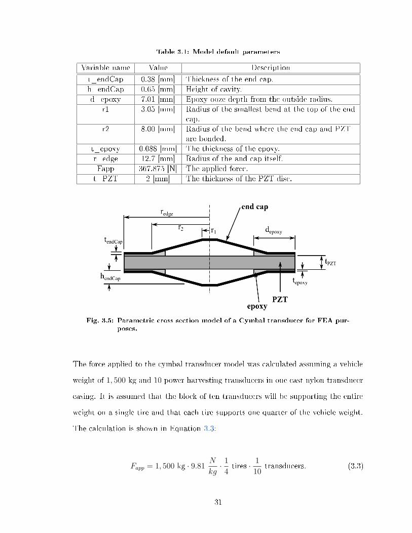
1, 500
Fapp = 1, 500 · 9.81 N
kg· 14
· 1
10.

In order to perform FEA on a geometry, the assembly must be reduced to a series
of nite elements. The density of these elements roughly correlates to the intricacy
of the analysis that the model is capable of. Unless otherwise stated, the model was
meshed such that the features of the model, especially small ones such as the epoxy
layer and epoxy ooze shown in Figure 3.5, were spanned by several nite elements.
This was done to ensure accuracy at the expense of computation time. The basic
mesh assigned to the default geometry is shown in Figure 3.6.
Fig. 3.6: FEA geometry mesh.
Governing equations for the FEA model were dened in Chapter 1: Introduction as
Equations Piezoelectric notation and Piezoelectric notation but are repeated here for
clarity.
x = cEX − eESE (3.4)
D = eESX + εE (3.5)
32

where cE , eES, and ε are material properties dened in Section 3.2.1. E is the
applied electric eld, X is the strain, x is the internal stress, and D is the surface
charge density. These equations apply to the piezoelectric material component of
the model only, shown in Figure 3.5. The rest of the material follows the governing
equations derived from Hooke's law:
x = YxyX (3.6)
where Yxy is the materials Young's modulus and can be related to the elastic compli-
ance with Equation 1.18.
All axisymmetric models applied the symmetry axis about the red line in Figure 3.6
and bounded the bottom edge of the model to only displace radially (a symmetric
constraint). The load, shown in Table 3.1, is applied to the model as an evenly
distributed load to the top edge of the model.
3.2.1 Material selection
The materials used in the model along with their properties are shown in Table 3.2.
33
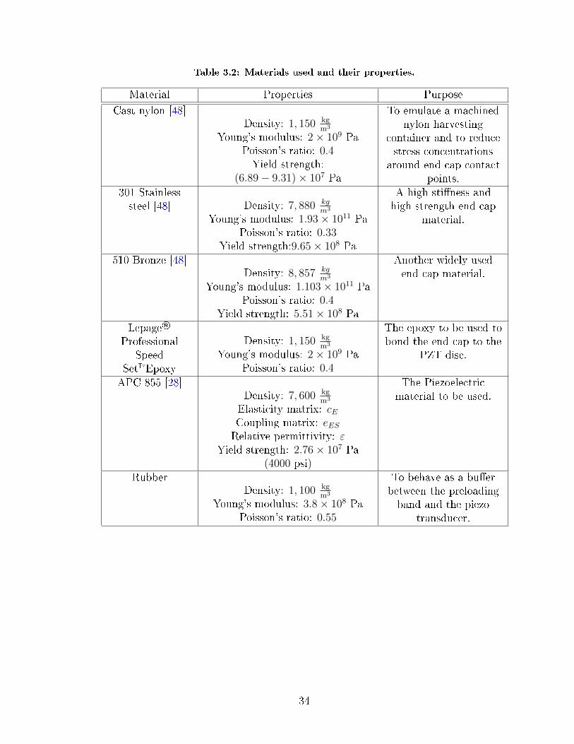
Table 3.2: Materials used and their properties.
Material Properties Purpose
Cast nylon [48]Density: 1, 150 kg
m3
Young's modulus: 2× 10⁹ PaPoisson's ratio: 0.4Yield strength:
(6.89− 9.31)× 107 Pa
To emulate a machinednylon harvesting
container and to reducestress concentrations
around end cap contactpoints.
301 Stainlesssteel [48] Density: 7, 880 kg
m3
Young's modulus: 1.93× 10¹¹ PaPoisson's ratio: 0.33
Yield strength:9.65× 10⁸ Pa
A high stiness andhigh strength end cap
material.
510 Bronze [48]Density: 8, 857 kg
m3
Young's modulus: 1.103× 10¹¹ PaPoisson's ratio: 0.4
Yield strength: 5.51× 10⁸ Pa
Another widely usedend cap material.
Lepage®
ProfessionalSpeed
SetEpoxy
Density: 1, 150 kgm3
Young's modulus: 2× 10⁹ PaPoisson's ratio: 0.4
The epoxy to be used tobond the end cap to the
PZT disc.
APC 855 [28]Density: 7, 600 kg
m3
Elasticity matrix: cECoupling matrix: eESRelative permittivity: ε
Yield strength: 2.76× 10⁷ Pa(4000 psi)
The Piezoelectricmaterial to be used.
RubberDensity: 1, 100 kg
m3
Young's modulus: 3.8× 10⁸ PaPoisson's ratio: 0.55
To behave as a buerbetween the preloadingband and the piezo
transducer.
34
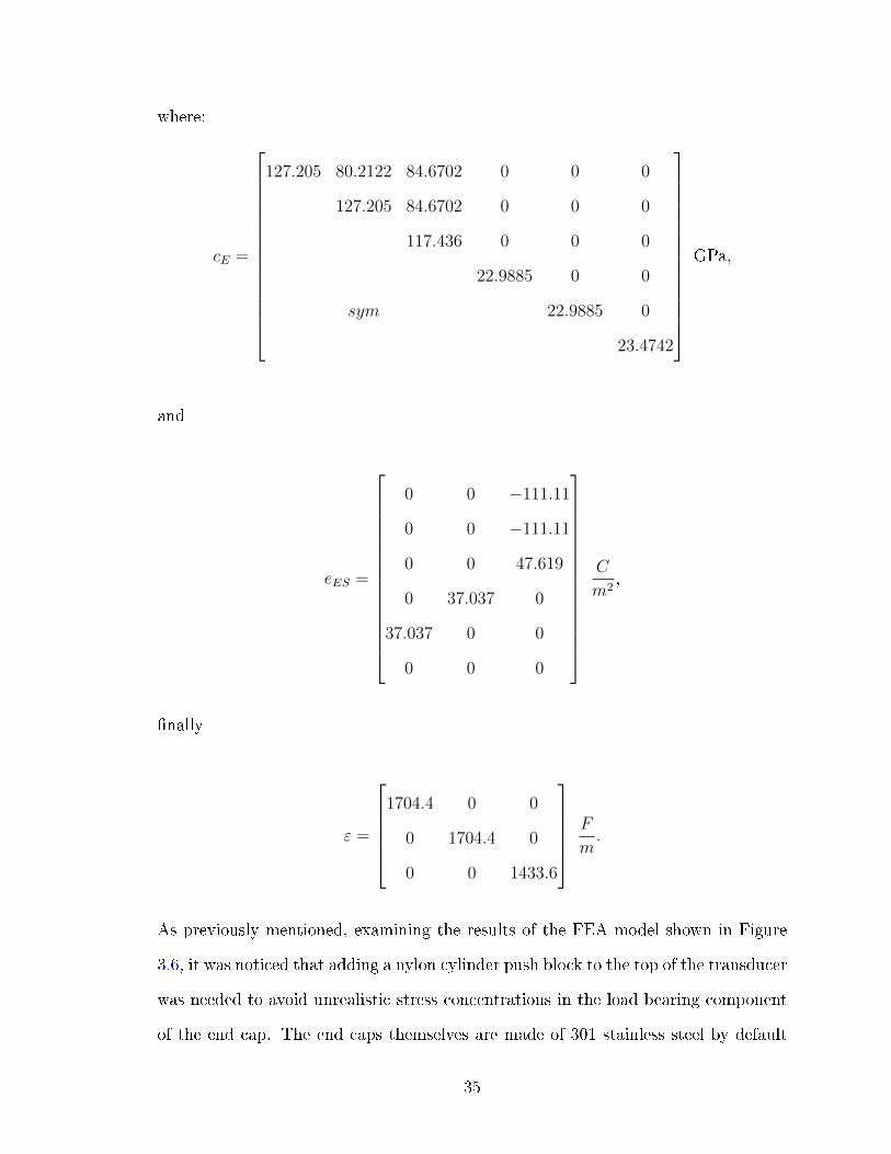
where:
cE =
127.205 80.2122 84.6702 0 0 0
127.205 84.6702 0 0 0
117.436 0 0 0
22.9885 0 0
sym 22.9885 0
23.4742
GPa,
and
eES =
0 0 −111.11
0 0 −111.11
0 0 47.619
0 37.037 0
37.037 0 0
0 0 0
C
m2,
nally
ε =
1704.4 0 0
0 1704.4 0
0 0 1433.6
F
m.
As previously mentioned, examining the results of the FEA model shown in Figure
3.6, it was noticed that adding a nylon cylinder push block to the top of the transducer
was needed to avoid unrealistic stress concentrations in the load bearing component
of the end cap. The end caps themselves are made of 301 stainless steel by default
35

in the models because the material is very strong, and can withstand smaller end
cap thicknesses. The 510 bronze, also known as phosphor bronze, was used in other
transducer designs [24, 38, 41, 49], and in our initial prototypes. The Lepage® Pro-
fessional Speed SetEpoxy proved to be a capable adhesive in early prototypes, and
so was used in the modeling. APC 855 was used due to reasons described in Section
2.2 and nally, the rubber was used as a buer, reducing stress concentrations, and
allowing the transducer to expand in the model.
3.2.2 Endcap thickness model
In order to determine the eect of end cap thickness on the output power produced,
the model was set up to step through a range of possible end cap thicknesses using
301 stainless steel end caps. This is the material that will later be chosen for use on
the nal prototypes due to its high stiness and yield strength. The thickness ranged
from 0.0254 mm to 0.381 mm with a step size of 0.0254 m. These correspond to a
step size and initial thickness of 0.001” (0.0254 mm) and a nal thickness of 0.015”
(0.381 mm) as the thicknesses available for purchase tend to be in imperial units and
thus in thousandths of an inch [48]. The maximum stress in the PZT material, the
end cap material, and total electric energy from the model was recorded and is plotted
against end cap thickness in Figures 3.7, 3.8, and 3.9, respectively.
36

Fig. 3.7: Maximum calculated stress in the stainless steel end cap.
Fig. 3.8: Maximum calculated stress in the piezo disc.
Fig. 3.9: Total electric energy produced under compression.
37

From these models, it can be seen that a solid end cap thickness of about 0.008”
(0.2032 mm) has the highest potential to produce the most electricity however it
results in the maximum stress of the PZT material that exceeds its yield strength.
This result is later tested with fabricated prototypes. It is noted that the range of
peak stresses shown in Figure 3.8 are all above the failure strength which was reported
by the manufacturer, APC, which reported it as being between 2, 000 and 4, 000 psi
(13.8 MPa−27.6 MPa) in tension and 6, 000 and 8, 000 psi (41.4 MPa−55.2 MPa) in
compression. Transducers prototyped, built, and tested in Chapter 4 have performed
well without damage to the PZT disc, indicating that the reported failure values
may have a safety factor associated with them. Although preloading methods will
be explored later in this paper to reduce the peak stresses below the maximums
suggested by APC, the largest end cap thickness of 0.015” (0.381 mm) is chosen as a
conservative parameter value.
3.2.3 Epoxy ooze model
It was noticed when deconstructing old cymbal transducer prototypes that often a
large amount of epoxy had oozed into the central cavity. It was decided to simulate
this phenomenon in order to see if it has a signicant eect on the cymbals power
production and internal stresses. The model varied the depth of epoxy ooze from
having no ooze (just epoxy where the end cap would contact the piezoelectric ma-
terial) to the point where the epoxy lled into the cavity up to the smaller radius
bend, truncating the cymbals cone. This was simulated assuming the default model
thickness for the end cap.
The stresses in the end cap and PZT are shown in Figures 3.10, and 3.11. More
importantly however, the total power generated is shown in Figure 3.12 which shows
that there is an inverse relationship between epoxy ooze and electrical energy gener-
38

ated. This indicated that transducers must be built consistently with as little epoxy
ooze as possible.
Fig. 3.10: Maximum stress in the end cap while varying the ooze depth.
Fig. 3.11: Max stress in the piezo material while varying ooze depth.
39

Fig. 3.12: Electrical energy generated as a function of ooze depth.
The simulation was repeated with smaller end cap thicknesses, which resulted in
similar shaped electrical energy plots as shown in Figure 3.12. This indicates that
the epoxy ooze depth into the central cavity should be kept to a minimum to maintain
transducer performance. This analysis caused prototypes to be manufactured with
care to use as little epoxy as needed to reduce epoxy ooze and degraded transducer
performance as much as possible.
3.2.4 FEA preload model
Qualitatively, the preload model initially showed little improvement in reducing the
peak stress in the PZT material. Upon further inspection, it appeared that the
simulated metal band (which was placed adjacent to the PZT disc) was causing
stress concentrations to form between it and the PZT disc and negating its peak
stress reduction. A preload band directly contacting a transducer could cause a short
circuit, reducing charge generation. A buer band was added to the model with an
estimated Young's modulus, calculated from rubber stretch tests described later in
this section. This modication led to a large improvement in reduction of stress on the
PZT disc. As the Young's modulus of the band material was decreased (simulating a
40

softer, more pliable material), the ideal preload stress was found to increase. It has
made the study of preloading dicult as the ideal amount of preload stress seems
highly dependent on how hard the buering material is between the preload band
and the PZT disc.
The simulation indicates that the buer banding should be a very pliable material
such as rubber, and that the preload stress can be quite high with such a pliable
material. The preload model used an updated set of default model parameters shown
in Table 3.3 for the parametric model shown in Figure 3.5 which are the result of
more careful measurements being taken of disassembled transducers. In addition, the
preload model incorporated a preload band and buering rubber band. The preload
band was chosen to be 0.5 mm thick however any thickness would have been sucient
as the important information desired from the model is optimal preload stress. The
rubber buer layer's thickness was obtained from measurements of the diameter of
the cymbal transducer with three rubber bands around it. The rubber bands chosen
were originally designed for holding lobster claws closed. This type of band was
chosen because of their high thickness, ample height large enough to accommodate
the thickness of one or two transducers, and circular diameter smaller than one inch so
that they would encircle a 1 PZT transducer without slack. Three bands were chosen
due to a compromise between the transducer size and the improved performance of
having more bung material. The updated parameters, however, did not incorporate
a smaller epoxy ooze depth measurement, d_epoxy, due to the instability it caused
in the nonlinear model.
41

Table 3.3: Model updated default parameters.
Variable Name Value Description
t_endCap 0.38 [mm] Thickness of the end caph_endCap 0.62 [mm] Height of cavityd_epoxy 7.01 [mm] Epoxy ooze depth from the outside radiusr1 3.34 [mm] Radius of the smallest bend at the top of the end
capr2 7.97 [mm] Radius of the bend where the end cap and PZT
are bondedt_epoxy 0.079 [mm] The thickness of the epoxyr_edge 12.7 [mm] Radius of the and cap itselfFapp 367.875 [N] The applied forcet_PZT 1 [mm] The thickness of half of the PZT disct_rubb 2.45 [mm] Thickness of the preload rubbert_band 0.5 [mm] Thickness of the end cap preload band
In order to derive an estimate for the elastic modulus of the rubber, the elastics were
warped around two small metal bars, one was xed to a table, the other for attaching
weights to. The rubber elastics were measured to be 27.96 mm long (attened with
no load), 24.60 mm with no weight on the test rig, 40.90 mm with a single kilogram
mass, and 64.62 mm with a two kilogram mass. The elastic is measured to be 1.55 mm
thick and 12.28 mm wide. The cross sectional area is then calculated as 1.55 mm ·1 m
1,000 mm· 12.28 mm · 1 m
1,000 mm= 1.9034× 10⁻⁹ m2. The Young's modulus is dened as
E = F/A0
∆L/L0[32] so using the stretched measurements gathered, the elastic modulus
becomes:
E1 =9.81/ (2 · 1.9034× 10−9)
((40.9− 24.6)/24.6)/1000= 3.8892× 10⁸ Pa
E2 =(2 · 9.81) / (2 · 1.9034× 10−9)
((64.62− 24.6)/24.6)/1000= 3.1681× 10⁸ Pa
The preloaded transducer was modeled using structural nonlinearities since the ge-
ometry changed signicantly due to the exing of the end cap and compression of the
42

x0 =
⎡⎢⎢⎢⎢⎣
0 0 0
0 0 0
0 0 −xprld
⎤⎥⎥⎥⎥⎦
xprld
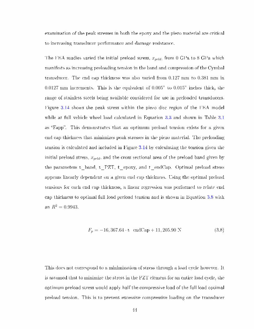
examination of the peak stresses in both the epoxy and the piezo material are critical
to increasing transducer performance and damage resistance.
The FEA studies varied the initial preload stress, xprld, from 0 GPa to 8 GPa which
manifests as increasing preloading tension in the band and compression of the Cymbal
transducer. The end cap thickness was also varied from 0.127 mm to 0.381 mm in
0.0127 mm increments. This is the equivalent of 0.005” to 0.015” inches thick, the
range of stainless steels being available considered for use in preloaded transducers.
Figure 3.14 shows the peak stress within the piezo disc region of the FEA model
while at full vehicle wheel load calculated in Equation 3.3 and shown in Table 3.1
as Fapp. This demonstrates that an optimum preload tension exists for a given
end cap thickness that minimizes peak stresses in the piezo material. The preloading
tension is calculated and included in Figure 3.14 by calculating the tension given the
initial preload stress, xprld, and the cross sectional area of the preload band given by
the parameters t_band, t_PZT, t_epoxy, and t_endCap. Optimal preload stress
appears linearly dependent on a given end cap thickness. Using the optimal preload
tensions for each end cap thickness, a linear regression was performed to relate end
cap thickness to optimal full load preload tension and is shown in Equation 3.8 with
an R2 = 0.9943.
Fp = −16, 367.64 · t_endCap + 11, 205.90 N (3.8)
This does not correspond to a minimization of stress through a load cycle however. It
is assumed that to minimize the stress in the PZT element for an entire load cycle, the
optimum preload stress would apply half the compressive load of the full load optimal
preload tension. This is to prevent excessive compressive loading on the transducer
44

while it is unloaded.
Fig. 3.14: Peak piezo material stress for the range of end cap thicknesses andpreload tensions examined.
Because of the susceptibility of the epoxy to fail, consideration was also given to
examining the peak stress in the epoxy region under the same range of preloading
and end cap thicknesses. Figure 3.15 shows those peak stresses, which indicates that
for the range of preload and end cap thickness cases solved, the stress within the epoxy
bond is reduced with increased preload tension and increased end cap thickness.
Fig. 3.15: Peak stress in the epoxy region of the model in a range of and capthicknesses and preload tensions tested.
Finally the eect of preloading and end cap thickness on the end caps peak stress was
45

examined and the results are shown in Figure 3.16. Although the preload seems to
have little eect on the peak end cap stress, it does has the eect of reducing the peak
stress experienced by the end cap. The largest determiner of stress on end caps is the
end cap thickness with smaller end cap thicknesses drastically increasing internal end
cap stresses, preload tension, and very slightly reducing internal stresses. Referencing
Table 3.2 the thinnest safe end cap thickness would be 0.2032 mm or 0.008 thick.
These results indicate that preloading can be used to reduce the peak piezoelectric
and end cap materials stresses and is explored with prototypes later in this thesis.
Fig. 3.16: Peak stress in the stainless steel end cap region of the model in arange of and cap thicknesses and preload tensions.
3.2.5 Analytical preload model
Due to the very large nite elements in the FEA model, an analytic model as created
to verify the FEA results. In order to place an upper bound the preload tension
needed, a model is devised where the end cap is divided into N thin wedges where
cylindrical stresses are ignored. The introduction of cylindrical stresses to the model
would reduce the amount of preloading required due to the end caps applying a
circumferential tension, supplementing the preloading tension. One of these extremely
46

Fr =r2 − r1hendCap
(Fapp
N
)
Fr
Ft Fr
Ft =Fr
2 sin(πN
)
Ft =
r2−r1hendCap
(Fapp
N
)2 sin
(πN
) .

θ
N → ∞ Ft
limN→∞
Ft =(r2 − r1)Fapp
2πhendCap
.
438.41

for preload band tension, calculated to be 438.41 N, can be compared to the lowest
estimate given by Equation 3.8 which is calculated as 4969.8 N assuming an end cap
thickness of 0.381 mm. The large discrepancy between the analytical solution and
the FEA solution may indicate that the mesh density in the preload FEA model is
likely too low and the numerical results from that study are unlikely to be accurate.
3.2.6 Slit model
The ultimate goal of the FEA slitted model was to determine the eect and appropri-
ate number of radial slits in a cymbal transducer design. The paper in [43] performed
analysis of similarly radially slitted cymbal transducers, examining both an analytic
model and FEA model. They however made the assumption that the radial slits
would be very thin. It was decided that the easiest way to cut thin radial slots in
the stainless steel end caps was to use a water jet cutting machine. The cutting
machine is capable of cutting slots 0.045 or 1.77 mm in width. This minimum slot
width constraint is then used as the models slot width. Though small, this width
is not insignicant and large number of slots (24 slots) which are examined in the
study [43] become infeasible when the tops of the slots would connect and cause the
top of the end cap to become disconnected from the rest of the end cap. In order
to simulate radial slits in an end cap, the model must be made in three dimensions.
Using symmetry boundary conditions, the number of elements in the model can be
drastically reduced for ease of simulation. For example, the six slit transducer tested
on the MTS machine could be simulated using 12 fold symmetry shown in Figure
3.19.
49

θ = 180/
θ
6.01
0.015” (0.381 )
0.010” (0.254 )
2.76×10⁷
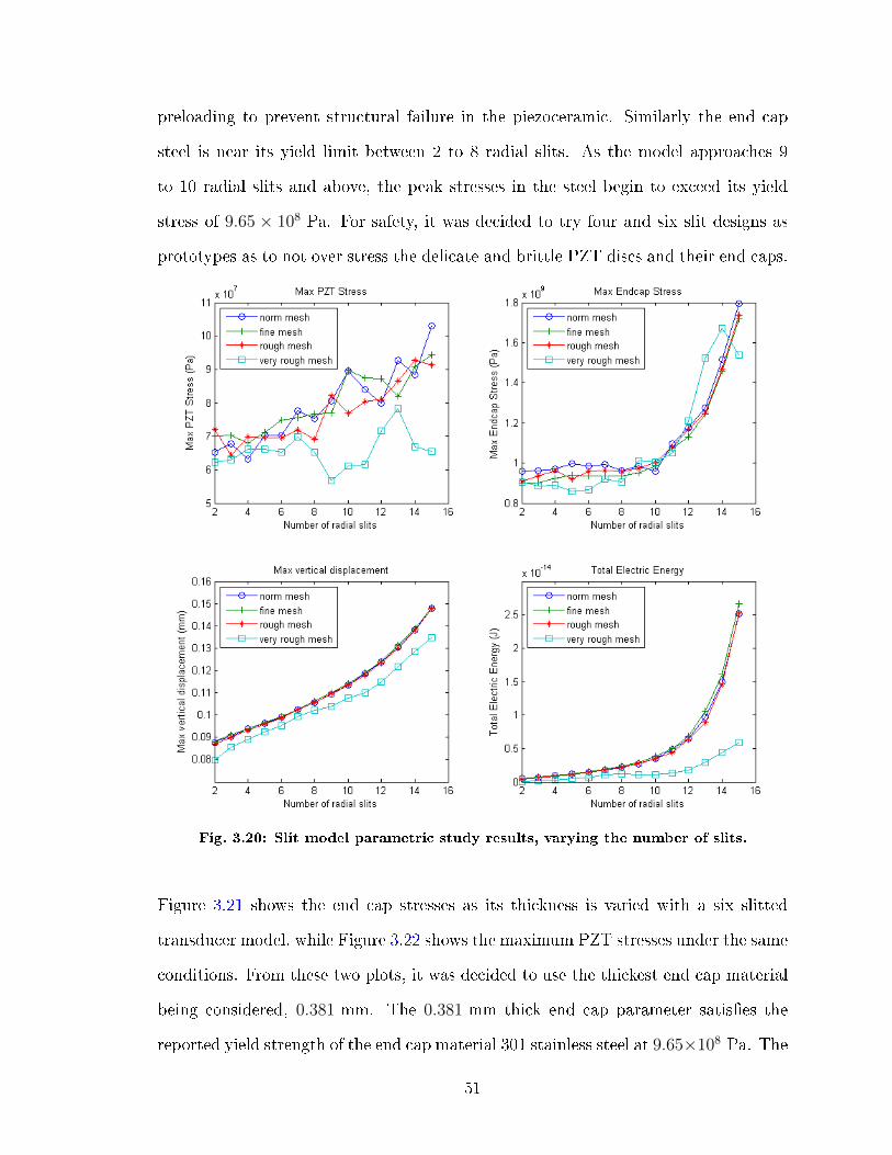
preloading to prevent structural failure in the piezoceramic. Similarly the end cap
steel is near its yield limit between 2 to 8 radial slits. As the model approaches 9
to 10 radial slits and above, the peak stresses in the steel begin to exceed its yield
stress of 9.65 × 10⁸ Pa. For safety, it was decided to try four and six slit designs as
prototypes as to not over stress the delicate and brittle PZT discs and their end caps.
Fig. 3.20: Slit model parametric study results, varying the number of slits.
Figure 3.21 shows the end cap stresses as its thickness is varied with a six slitted
transducer model, while Figure 3.22 shows the maximum PZT stresses under the same
conditions. From these two plots, it was decided to use the thickest end cap material
being considered, 0.381 mm. The 0.381 mm thick end cap parameter satises the
reported yield strength of the end cap material 301 stainless steel at 9.65×10⁸ Pa. The
51

stresses for the PZT disc, shown in Figure 3.22, exceed the material yield strengths as
expected. The added radial slits appropriately amplify the forces on the piezoceramic
material which will be compensated for in practice by preloading. A prototype with
too many slots may experience yielding or failure within the end caps of the transducer
and as a result of these FEA results, it was decided to manufacture four and six slitted
end capped prototypes to be compared and preloaded.
Fig. 3.21: Maximum end cap stresses in the slit model plotted against end capthickness.
Fig. 3.22: Maximum PZT stresses in the slit model plotted against end capthickness.
52

3.3 FEA conclusions
From the work performed in the previous section, it was decided that the nal pro-
totypes for the novel transducer design will have to have a 0.015” (0.381 mm) thick
stainless steel end cap because of the materials strength and because of the stress con-
centrations introduced from adding radial slits. The prototypes must be preloaded
using half of the ideal preload tension of 438.41 N2
= 219.21 N at full design load of
367.875 N. Given the results and increased stress concentrations from adding radial
slits, the nal prototypes will have either 4 or 6 radial slots which will be tested and
compared as only 0.013” (0.3302 mm) thick end caps will be able to survive the load
with six radial slits. Finally the transducers must be manufactured with as little
epoxy ooze as possible to avoid poor transducer performance.
Attempts at creating a model incorporating both radially slitted end caps and preload-
ing caused instabilities. Prototypes of the modeled transducers along with experi-
ments were then used to verify the conclusions made here and are discussed in the
following chapter.
53

4 Implementation and testing
4.1 Initial transducer designs
4.1.1 Bridge transducer
Initially simple bridge and cymbal transducers were manufactured as were compared
in [38]. Figure 4.1 shows a bridge transducer which was constructed for comparison
with our early cymbal transducer designs. A potential benet of the Bridge transducer
could be an increased capacity to generate electricity due to a larger amount of
piezoceramic material per transducer, which translates into more surface area for
charge to be generated, when compared to a cymbal transducer of the same diameter.
Another benet would be fewer power losses due to less strain energy lost to end cap
deformation since the end cap material would not have to expand cylindrically like
the cymbal transducer. Like [38] however, it was found that the Bridge transducers
are much less structurally stable than the Cymbal transducer and that the Bridge
transducers were prone to structural failure of the PZT plate.
Fig. 4.1: Bridge transducer.
4.1.2 Cymbal transducer
Cymbal transducers are manufactured by fabricating metal end caps which are then
adhered to a piezoelectric disc. The construction of the end caps and their connection
to the PZT discs then becomes the main challenge in the transducers assembly. First,
stainless steel or bronze discs are punched out of a sheet using a disc cutter. These
54

discs are then fed into a custom machined die attached to a die set shown in Figure
4.2. The additional male and female die in the right hand side of Figure 4.2 are for
punching metal squares into bridge transducers. The die is placed in a manual press
shown in Figure 4.3 and stamps the metal discs into the desired end cap shape. Finally
the completed end caps are adhered to the piezoceramic discs using a stronger non
conductive epoxy and a small amount of weaker silver conductive epoxy to improve
ease and reliability of wiring.
Fig. 4.2: Cymbal end cap male and female dies attached to a die set (center-left) with bridge dies (right).
Fig. 4.3: Manual press for operating the die set.
55

Once it was decided what type transducer was to be used, a simple harvester was
constructed using 9 pairs of Cymbal transducers. Shown in Figure 4.4, the 3×3 power
harvester is composed of 18 transducers in total. The Cymbal transducers stacked
in pairs to improve the amount of electric charge generation. The power generated
along with the harvesting pad thickness and the amount the pad will be displaced
when compressed can be tuned by stacking many transducers vertically. The 1
diameter transducers were designed to collectively harvest power from the full design
load of an approximately 1, 500 kg vehicle and were placed in a machined nylon block
to support and protect the transducers. The nylon block, housing the transducers,
included grooves and additional holes machined into it for wiring purposes and for
the attachment of diode rectiers. Nylon was used because of its machinability, low
cost, dielectric properties, water resistance, and rigidity. Each transducer pair was
connected in parallel and then connected to the main power bus using the diode
rectiers. By isolating the transducer pairs with the rectiers, charge that would be
lost due to the inverse piezoelectric eect caused by uneven loading of the harvesting
pad is avoided.
Fig. 4.4: Early tested vehicle harvester.
The depth of the nylon pockets were machined according to FEA estimates of the
56
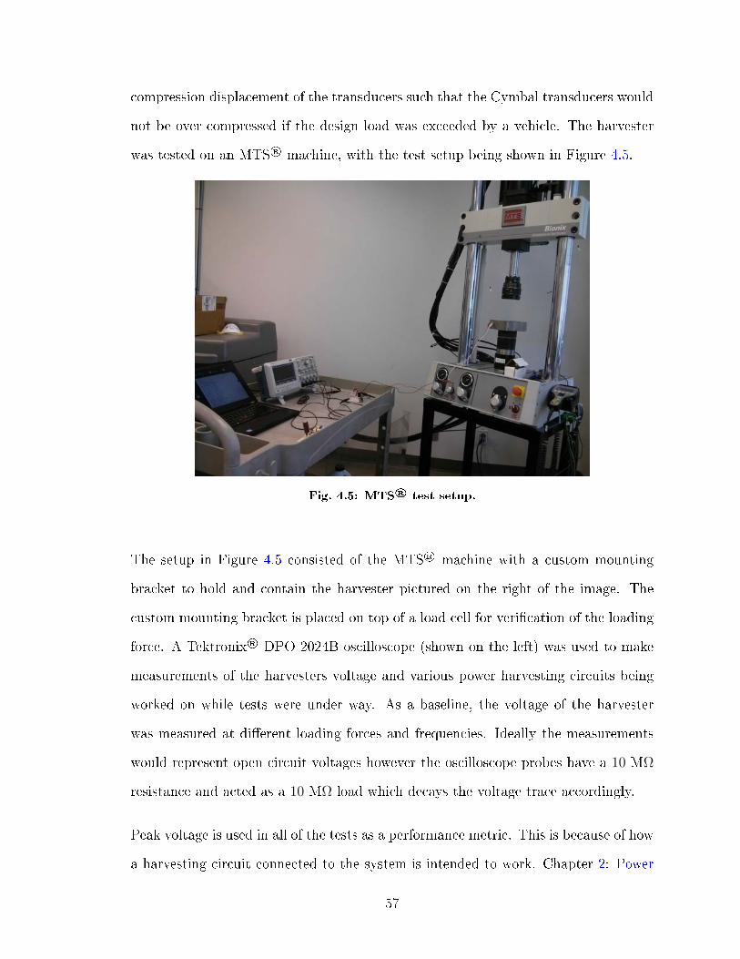
compression displacement of the transducers such that the Cymbal transducers would
not be over compressed if the design load was exceeded by a vehicle. The harvester
was tested on an MTS® machine, with the test setup being shown in Figure 4.5.
Fig. 4.5: MTS® test setup.
The setup in Figure 4.5 consisted of the MTS® machine with a custom mounting
bracket to hold and contain the harvester pictured on the right of the image. The
custom mounting bracket is placed on top of a load cell for verication of the loading
force. A Tektronix® DPO 2024B oscilloscope (shown on the left) was used to make
measurements of the harvesters voltage and various power harvesting circuits being
worked on while tests were under way. As a baseline, the voltage of the harvester
was measured at dierent loading forces and frequencies. Ideally the measurements
would represent open circuit voltages however the oscilloscope probes have a 10 MΩ
resistance and acted as a 10 MΩ load which decays the voltage trace accordingly.
Peak voltage is used in all of the tests as a performance metric. This is because of how
a harvesting circuit connected to the system is intended to work. Chapter 2: Power
57

harvesting electronics outlines a harvesting circuit model which makes use of peak
voltage detection. When this circuit detects a peak voltage, the energy stored in the
piezoelectric material is discharged into the circuit. The amount of energy available
to the circuit for harvesting is represented by Equation 2.2, E = 12CV 2, which is a
function of peak transducer voltage and its capacitance. Since the piezoelectric discs,
and therefore the transducer capacitance, are standardized between transducers, then
the peak voltage becomes a sole metric for transducer performance.
Figure 4.6 shows the traces produced by the harvester at 1 and 2 kN loads for ex-
citation frequencies 0.25, 0.5, and 1 Hz. The peak voltages of these traces where
measured and are displayed in Table 4.1. A simple equation for estimating power
consumed, or more accurately power dissipated by a load is proposed in [50] and is
shown in Equation 4.1.
P =V 2rms
R(4.1)
Fig. 4.6: Example harvester traces measured during the MTS® tests.
58

Table 4.1: Harvester MTS® machine test peak voltage results.
0.25 Hz 0.5 Hz 1 Hz1 kN 124− 66 V 92− 84 V 130− 124 V2 kN 92− 92 V 140− 140 V 162− 160 V3 kN - - 162− 160 V
Using Equation 4.1 and the oscilloscope probe resistance, the dissipated power is cal-
culated and tabulated in Table 4.2. This power represents the amount of available
electrical power that would be available to a load connected directly to the piezoelec-
tric harvesting pad.
Table 4.2: Harvester MTS® machine test power dissipation results.
0.25 Hz 0.5 Hz 1 Hz1 kN 0.161 mW 0.298 mW 0.599 mW2 kN 0.241 mW 0.542 mW 0.921 mW3 kN - - 0.984 mW
4.2 Comparison of slitted and solid endcapped transducers
In order to measure the performance of novel transducer designs compared with con-
ventional designs, a series of iterative experiments were performed on an MTS®
machine pictured in Figure 4.5.
4.2.1 Initial feasibility testing
The initial experiments which were performed with individual transducers on the the
MTS® machine setup shown in Figure 4.5, set up to use a force feedback mode to
apply a 0 N to 400 N sinusoidal load, above the 367.875 N design load in order to test
the transducers at their feasible limits. Each transducer was inserted into a cast and
machined nylon housing to protect it during testing (shown in Figure 4.7) and placed
59

on top of the custom bracket used in earlier tests. The rightmost block in Figure 4.7
is used for simple cymbal transducers with and without radial slitting and preloading,
and the center container is used to test cymbal transducers with preloading which
require more space. The cover for the blocks, on which the load is applied is shown
on the left.
Fig. 4.7: Machined cast nylon individual transducer test housing.
In order to compare the dierences between a solid endcapped transducer and one
with four slits each, two pairs, for a total of four transducers were manufactured with
one pair having four radial slits in its end caps and the other with non-slitted endcaps.
One transducer from each pair is shown in Figure 4.8). The four 0.015” (0.381 mm)
thick end caps were made with 301 stainless steel with material properties shown in
Table 3.2. One transducer from each pair was adhered to the piezoceramic disc using
Devcon® 5 minute® epoxy gel, and were labeled Slitted and solid Transducer 1
while the other two were attached using Lepage® professional speed set epoxy, and
labeled Slitted and solid Transducer 2, to examine the eects of dierent epoxies
on the transducer performances. The cycling frequency was set to 0.25 Hz as the
transducers are expected to operate in a low frequency manner of a traversing vehicle
every few seconds. The Cymbal units were connected directly to the oscilloscope to
measure the resulting voltage.
60
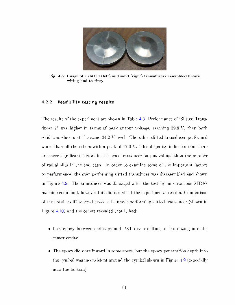
Fig. 4.8: Image of a slitted (left) and solid (right) transducers assembled beforewiring and testing.
4.2.2 Feasibility testing results
The results of the experiment are shown in Table 4.3. Performance of Slitted Trans-
ducer 2 was higher in terms of peak output voltage, reaching 39.8 V, than both
solid transducers at the same 34.2 V level. The other slitted transducer performed
worse than all the others with a peak of 17.0 V. This disparity indicates that there
are more signicant factors in the peak transducer output voltage than the number
of radial slits in the end caps. In order to examine some of the important factors
to performance, the over performing slitted transducer was disassembled and shown
in Figure 4.9. The transducer was damaged after the test by an erroneous MTS®
machine command, however this did not aect the experimental results. Comparison
of the notable dierences between the under performing slitted transducer (shown in
Figure 4.10) and the others revealed that it had:
Less epoxy between end caps and PZT disc resulting in less oozing into the
center cavity.
The epoxy did ooze inward in some spots, but the epoxy penetration depth into
the cymbal was inconsistent around the cymbal shown in Figure 4.9 (especially
near the bottom)
61

Used Lepage® professional speed set epoxy
The epoxy thickness looked consistently small between the outer edge of the
transducer and the end cap
Fig. 4.9: The over performing transducer, Slitted Transducer 2.
The other transducer, Slitted Transducer 1, shown in Figure 4.10 by contrast to the
other transducers had:
More epoxy ooze toward the central cavity
Was manufactured with more consistent epoxy placement
Used Devcon® 5 minute epoxy gel
Epoxy was much thicker in some areas causing small epoxy lled gaps between
the end cap and piezo disc
62

Fig. 4.10: The under performing transducer (Taken apart after the test), Slit-ted Transducer 1.
Analysis was performed on the oscilloscope trace data using MATLAB®. The trans-
ducers were connected to the oscilloscope directly through 10 MΩ leads. The cal-
culated power dissipated through the traces (shown in Figure 4.11) according to
Equation 4.1, as well as the peak voltage attained is shown in Table 4.3. The over
performing slitted transducer is labeled Slitted Transducer 2 in Table 4.3 while the
under performing one is labeled as Slitted Transducer 1.
Fig. 4.11: Traces of tested transducers during 1st test.
63

Table 4.3: Power dissipated by the oscilloscope, produced by transducers inthe 1st experiment.
Transducer Power (µW) Peak voltage (V)
Slitted Transducer 1 10.0 17.0− 16.6Slitted Transducer 2 60.3 39.8− 39.0Solid Transducer 1 26.6 34.2− 32.6Solid Transducer 2 42.1 34.2− 33.8
The two solid transducers have been manufactured the same ways as the slitted
transducers however one dissipated 58.6% more power than the other because it
sustained a high voltage after each voltage peak. This indicates that the Epoxy
contributes to the transducer charge dissipation performance. Part of the dierence
is also attributable to manufacturing consistency. Both of the solid transducers had
a large amount of epoxy ooze into the cavity in the end cap with Solid transducer 1
(shown in Figure 4.12) showing slightly less ooze than Solid transducer 2 (shown in
Figure 4.13). This indicates that the ooze depth may also be the cause of reduced
power generation as predicted by the epoxy ooze FEA study.
Fig. 4.12: One of the solid end capped transducers (Solid Transducer 1), takenapart after the test.
64

Fig. 4.13: The other solid end capped transducer (Solid Transducer 2) takenapart after the test (The PZT material cracked during disassembly).
4.2.3 Epoxy ooze experiment
To conrm the results of the FEA ooze parametric study, one solid and two slitted
transducers were built and shown in Figure 4.14. In order to attempt to get more
consistent and improved peak voltage, the harvesting units were built with less epoxy.
This test only used the Lepage® professional speed set epoxy which was applied
near the outside rim of the transducer end cap in order to reduce the amount of
ooze into the center cavity. During testing, both slitted transducers became partially
detached from the PZT material aecting the nal results and implying that too little
of an amount of epoxy was used and aected the resulting output power. The solid
transducer did not have this issue and was not damaged during the test.
65
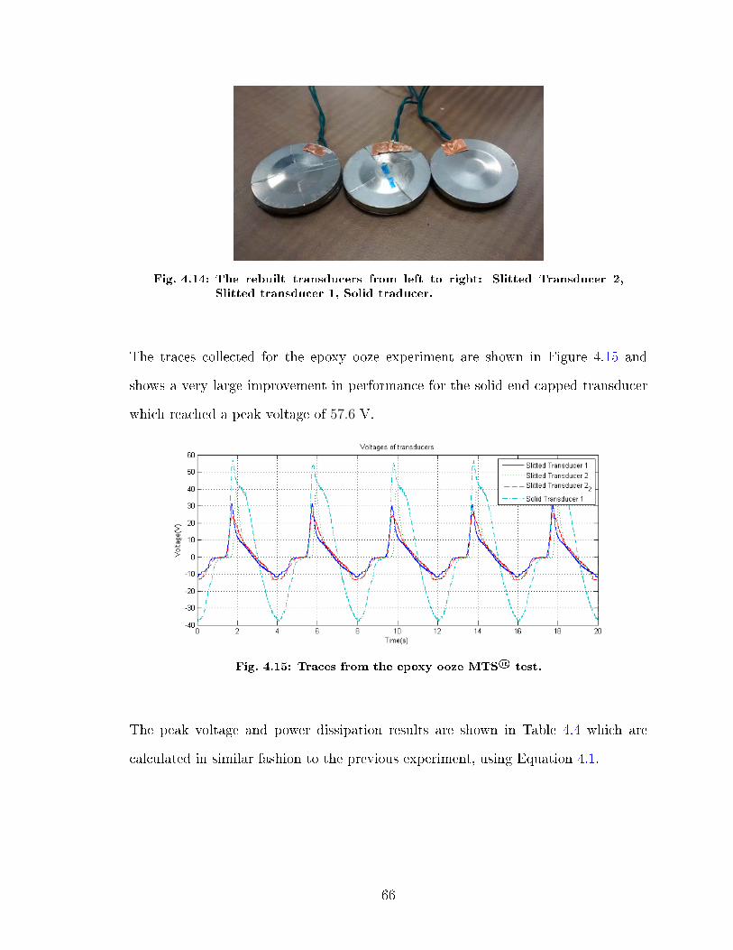
Fig. 4.14: The rebuilt transducers from left to right: Slitted Transducer 2,Slitted transducer 1, Solid traducer.
The traces collected for the epoxy ooze experiment are shown in Figure 4.15 and
shows a very large improvement in performance for the solid end capped transducer
which reached a peak voltage of 57.6 V.
Fig. 4.15: Traces from the epoxy ooze MTS® test.
The peak voltage and power dissipation results are shown in Table 4.4 which are
calculated in similar fashion to the previous experiment, using Equation 4.1.
66

Table 4.4: Power produced by the rebuilt transducers.
Transducer Power (µW) Peak voltage (V)
Slitted Transducer 1 8.78 31.2− 30.4Slitted Transducer 2 12.6 39.6− 38.8
Slitted Transducer 2 (run 2) 10.1 26.0− 24Solid Transducer 76.6 57.6− 55.2
The failure of both slitted transducers as the 400 N load was applied repeatedly is
the reason the power produced by both slitted transducers appears low compared
to the solid transducer in the experimental results in Table 4.4. Also, it is noted
that the solid transducer tested in this experiment produced a higher peak voltage
than the peak voltage from Slitted Transducer 2 , reaching 57.6 V compared to the
39.8 V measured during the previous test. This further indicates that manufacturing
inconsistency is the cause of the experimental result inconsistency of the transducers.
Images of the disassembled transducers are shown in Figures 4.16, 4.17, and 4.18 and
show inconsistent epoxy coverage as well as excessively applied conductive epoxy.
Meanwhile, the solid transducer that performed very well shows appropriately small
conductive epoxy application as well as a much more consistent and appropriate
amount of non-conductive epoxy.
Fig. 4.16: Slitted Transducer 1 after testing. The break seems to be caused bythe small patch without epoxy near the left edge of the end cap onthe right.
67
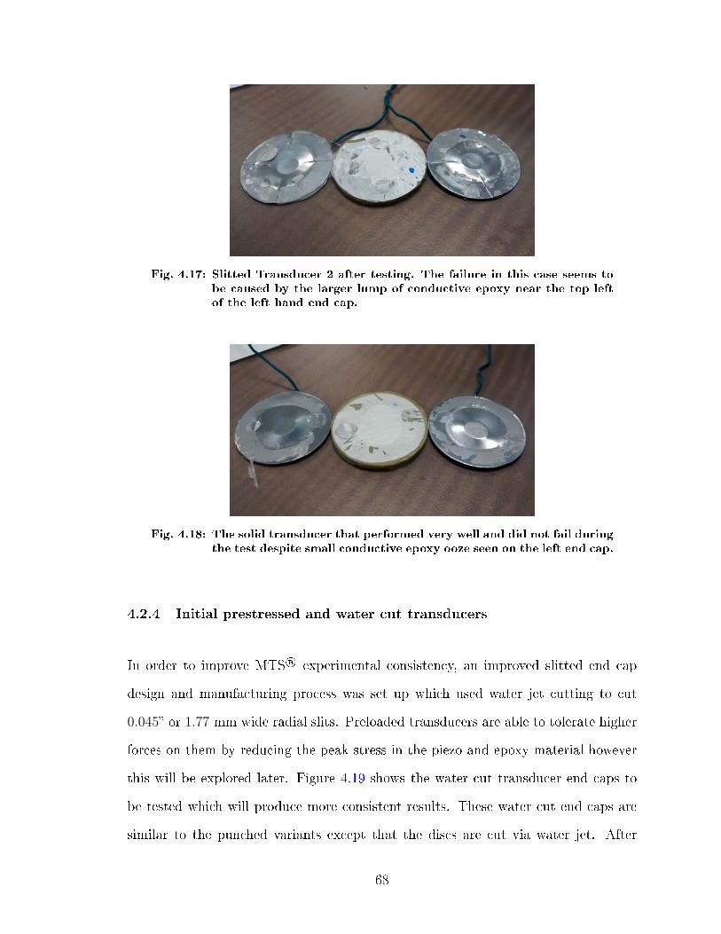
Fig. 4.17: Slitted Transducer 2 after testing. The failure in this case seems tobe caused by the larger lump of conductive epoxy near the top leftof the left hand end cap.
Fig. 4.18: The solid transducer that performed very well and did not fail duringthe test despite small conductive epoxy ooze seen on the left end cap.
4.2.4 Initial prestressed and water cut transducers
In order to improve MTS® experimental consistency, an improved slitted end cap
design and manufacturing process was set up which used water jet cutting to cut
0.045 or 1.77 mm wide radial slits. Preloaded transducers are able to tolerate higher
forces on them by reducing the peak stress in the piezo and epoxy material however
this will be explored later. Figure 4.19 shows the water cut transducer end caps to
be tested which will produce more consistent results. These water cut end caps are
similar to the punched variants except that the discs are cut via water jet. After
68

cutting, the discs are pressed in the cymbal die in order to give them their central
cavity. Six slits was chosen from the FEA analysis in the previous chapter as well as
four slit design to examine the dierence and potential experimentally.
Fig. 4.19: Six and four slit transducer end caps produced by water jet cuttingcompared to the plain versions on the right.
In order to test the damage resistant properties of preloading, four old phosphor
bronze transducers were used and are shown in Figure 4.20. Both preloaded and
non preloaded bronze transducers were subjected to an increasing load applied by
the MTS® machine until they reach their failure point. The bronze transducers on
the left of Figure 4.20 has an end cap thickness of 0.013 (0.330 mm) and the two in
the center have a thickness of 0.017 (0.432 mm). The two bronze transducers along
the top of the image are preloaded and the bottom units are not preloaded. If the
preloading works and is applying sucient pressure, the preloaded transducers will
take measurably more load to fail, while the non preloaded transducers will yield more
readily. On the right side of Figure 4.20 stainless steel transducers with four and six
slits are also prepared for testing. These slitted transducers use 0.015” (0.381 mm)
301 stainless steel for their end caps following the FEA study suggestion.
69

Fig. 4.20: Preloaded transducers next to their non-preloaded counterparts(left) and assembled water cut end cap slitted transducers (right).
Figure 4.21 shows the trace of the four slitted transducer which is shown in the bottom
right of Figure 4.20. The transducer performed well compared to earlier transducers,
dissipating 127.9 µW of power and reaching 89.2− 86.0 V at its peak.
Fig. 4.21: Trace of the four slit transducer.
The six slitted transducer's PZT disc fractured during the test and is shown disas-
sembled after the test in Figure 4.22. The failure of the piezoceramic indicates that
the radial slits are amplifying the radial stresses applied to the piezo material signif-
icantly more when compared to the other transducers tested, to the point of failure.
Following tests try to incorporate preloading in order to prevent such failures and
generate more power than the four slitted transducer design.
70

Fig. 4.22: The six slitted transducer after testing.
In order to test the eect of preloading on the failure load, an applied load was
slowly increased for the bronze solid endcapped transducers. Failure was estimated
through a combination of sharp force drop o detected by the MTS® machine's load
cell and listening for sharp cracking sounds indicating piezoceramic or epoxy failure.
The preloaded transducer with the 0.13 (0.330 mm) thick end cap was accidentally
loaded to 5 kN (shown in Figure 4.23) and so the specic force when failure occurred
could not be accurately attained.
Fig. 4.23: Preloaded transducer after 5 KN load.
Screen shots of the output of the MTS® machine were taken (shown in Figure 4.24
and 4.25) in order to show the loads at the suspected failure points of the preloaded
and non preloaded transducers. Failure points were identied by a sharp increase in
71
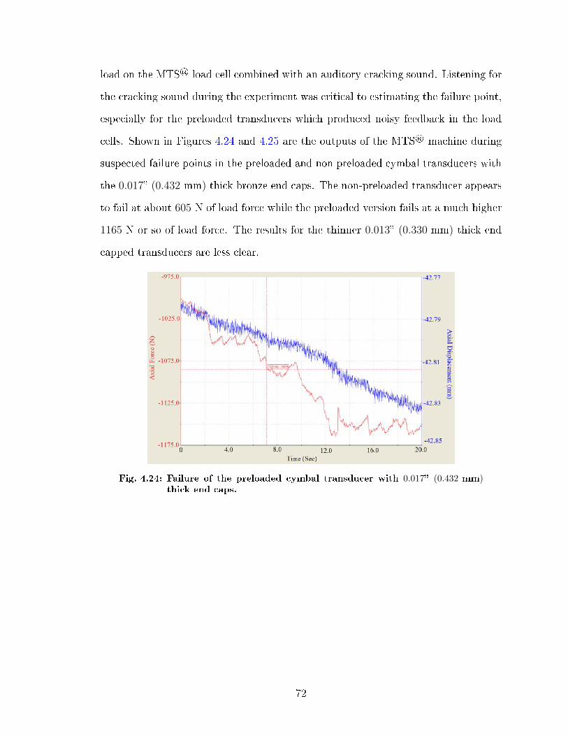
load on the MTS® load cell combined with an auditory cracking sound. Listening for
the cracking sound during the experiment was critical to estimating the failure point,
especially for the preloaded transducers which produced noisy feedback in the load
cells. Shown in Figures 4.24 and 4.25 are the outputs of the MTS® machine during
suspected failure points in the preloaded and non preloaded cymbal transducers with
the 0.017 (0.432 mm) thick bronze end caps. The non-preloaded transducer appears
to fail at about 605 N of load force while the preloaded version fails at a much higher
1165 N or so of load force. The results for the thinner 0.013 (0.330 mm) thick end
capped transducers are less clear.
Fig. 4.24: Failure of the preloaded cymbal transducer with 0.017 (0.432 mm)thick end caps.
72

Fig. 4.25: Failure of the non-preloaded cymbal transducer with 0.017(0.432 mm) thick end caps.
Figures 4.26, 4.27, and 4.28 show the results of the thinner 0.013 thick end cap
transducers during their failure MTS® test. There appeared to be two failure points
for the non-preloaded transducer. One failure point was at 975 N and the other
was around 1156 N of load. It is possible that the transducer failed in several spots
during the test in which case the lowest failure point should be chosen. The preloaded
version of the transducer was accidentally loaded very quickly as can be seen in the
bottom image of Figure 4.28. This accidental destruction of the test transducer, did
not prevent the measurement of a result which reached 4910 N. It may be the case,
similar to that of its non-preloaded counterpart, that the preloaded cymbal failed
at several load levels, however the loading rate was too high or the failure signs too
subtle, for the instrumentation to pick up on them.
73

Fig. 4.26: First failure of the non-preloaded, 0.013 (0.330 mm) transducer.
Fig. 4.27: Second failure of the non-preloaded, 0.013 (0.330 mm) transducer.
74

Fig. 4.28: Failure of the preloaded cymbal transducer with 0.013 (0.330 mm)thick end caps.
After the test, the transducers were examined and it was found that they seemed to be
intact including the brittle ceramic PZT disc. The perceived failures may be caused
by small cracks forming within the epoxy or the PZT. Transducers loaded to the
epoxy failure limit also represent a failure of the harvesting transducer even though
they may still produce some power. This establishes that preloading can improve the
damage resistance of transducers and is explored experimentally later.
4.2.5 Preloading of a slitted transducer
A new MTS® experiment was set up to determine whether preloading the transducer
with six radial slits (shown in Figure 4.22) would make it more resistant to failure
of the piezoceramic or bonding epoxy material. The goal of the test was to produce
a higher peak voltage than the piezo unit with four radial slits while not causing
a failure of the six slitted transducer shown in the bottom right corner of Figure
4.20. Figure 4.29 shows an image of the six slitted-preloaded transducer on the
right, and the same transducer in its test conguration on the left. Two aluminum
cylinders were machined and positioned so that the slitted cymbal transducer could be
75
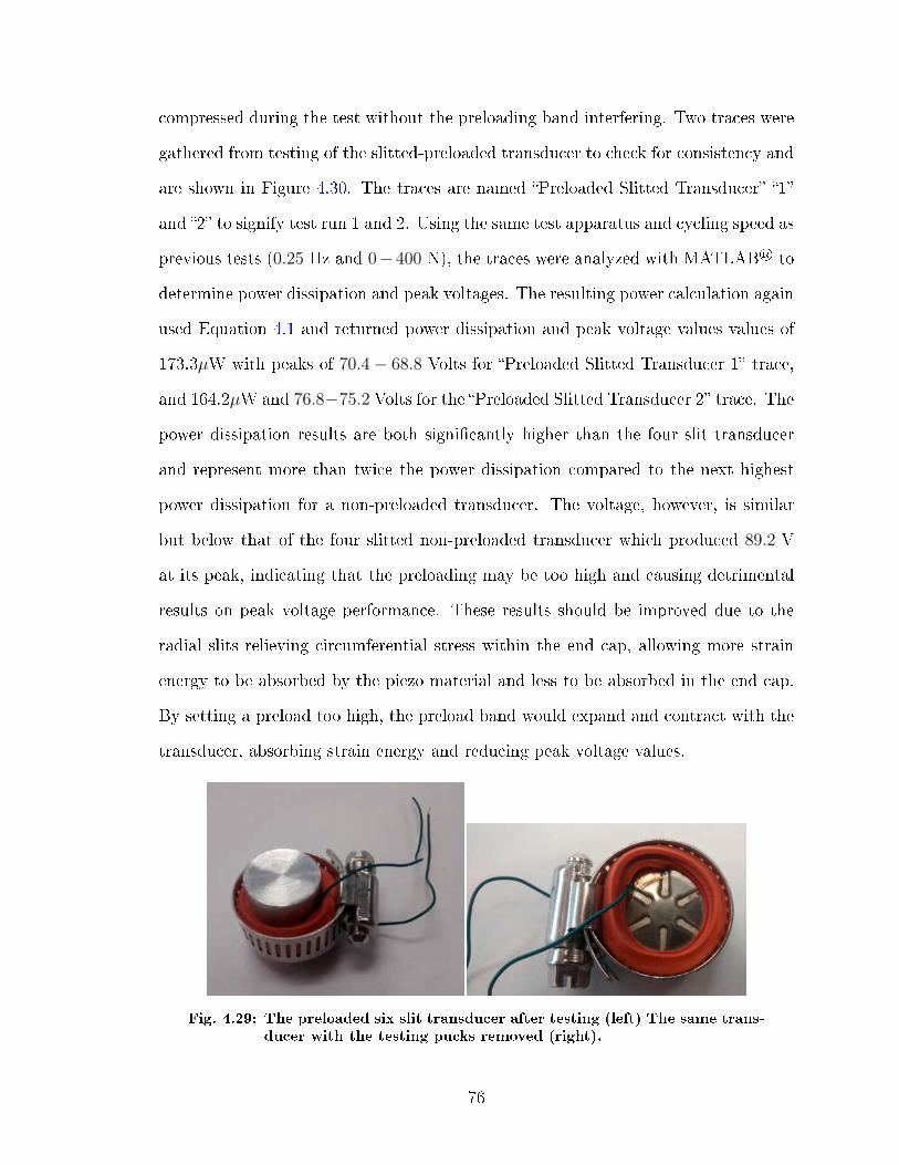
compressed during the test without the preloading band interfering. Two traces were
gathered from testing of the slitted-preloaded transducer to check for consistency and
are shown in Figure 4.30. The traces are named Preloaded Slitted Transducer 1
and 2 to signify test run 1 and 2. Using the same test apparatus and cycling speed as
previous tests (0.25 Hz and 0− 400 N), the traces were analyzed with MATLAB® to
determine power dissipation and peak voltages. The resulting power calculation again
used Equation 4.1 and returned power dissipation and peak voltage values values of
173.3µW with peaks of 70.4− 68.8 Volts for Preloaded Slitted Transducer 1 trace,
and 164.2µW and 76.8−75.2 Volts for the Preloaded Slitted Transducer 2 trace. The
power dissipation results are both signicantly higher than the four slit transducer
and represent more than twice the power dissipation compared to the next highest
power dissipation for a non-preloaded transducer. The voltage, however, is similar
but below that of the four slitted non-preloaded transducer which produced 89.2 V
at its peak, indicating that the preloading may be too high and causing detrimental
results on peak voltage performance. These results should be improved due to the
radial slits relieving circumferential stress within the end cap, allowing more strain
energy to be absorbed by the piezo material and less to be absorbed in the end cap.
By setting a preload too high, the preload band would expand and contract with the
transducer, absorbing strain energy and reducing peak voltage values.
Fig. 4.29: The preloaded six slit transducer after testing (left) The same trans-ducer with the testing pucks removed (right).
76

Fig. 4.30: Preloaded six slitted transducer trace.
4.2.6 Transducer loading and end cap material experiment
In order to properly compare a slitted and preloaded transducer to a solid end capped
one, an experiment was performed to explore design renements to the solid trans-
ducer. The purpose of this experiment was to determine weather 0.008 301 stainless
steel would be a better performing endcap compared to the 0.01” thick 510 phosphor
bronze used on some previous solid transducers as was suggested by the end cap
thickness FEA study. In addition, roughening of the end caps with sand paper was
used to improve adhesion between end cap and the epoxy. Finally peak voltage and
power dissipation where measured as larger forces were applied to the cymbal units to
understand the role of load on the piezoelectric harvesters. The rationale behind the
variations of end cap materials and thicknesses are as follows. The thickness of the
stainless steel end capped transducers was chosen from the FEA end cap thickness
studies performed in Chapter 3 while the thickness of the bronze transducers where
chosen because of their successful use in the rst roadway harvesting pad. The four
77

transducers, made and shown in Figure 4.31, are numbered 1 to 4 from the left. In
order to improve performance, the transducers were assembled with as little epoxy as
possible to prevent ooze into the central cavity.
Fig. 4.31: The solid end capped transducers after the MTS® test (numbered1-4 from the left).
Figure 4.32 shows the four transducers disassembled after the MTS® test. Transducer
1 had an end cap fall o during the test while transducer 3 had its end cap separate
slightly during the test. Due to careful assembly, all transducers had smaller amounts
of ooze than earlier transducers with transducer 1 having little but uniform ooze
into the central cavity. Predominantly failures occurred within the epoxy and metal
endcap interface, however when transducer 4 was taken apart, the epoxy separated
from the PZT disc. It is noted that the epoxy for transducers 1 and 3 were tinted
gray and the epoxy for transducers 2 and 4 were tinted reddish indicating that metal
powder from the roughing process was left on the end caps before assembly and
contributed to their failures.
78

Fig. 4.32: Solid transducers after testing with end caps removed (ordered 1-4from the left).
Table 4.5 shows the power calculated using Equation 4.1 and peak voltage for each
transducer under set sinusoidal loads. The MTS® machine tended to undershoot
the desired peak force level in the tests, and so the actual peak loading force is
reported instead of the desired loading force. The results show that the stainless
steel transducers appear to generate less power with increased load compared to the
bronze endcapped transducers despite performing much better at lower force ranges.
These results appear to be caused by partial or complete failure (as was the case with
transducer 1 and transducer 2) within the epoxy - endcap bond. It is noted that
the power dissipated and peak voltage produced by transducer 1 before failure was
greater than the best performing phosphor bronze transducer at much higher loads.
The highest performing tests for the phosphor bronze transducers generated power in
the high 70's and low 80's (µW) range and peak voltage in the low 50's range (shown
in Table 4.5b and d), compared to the pre-failure power dissipation of transducer 1
at 96.7(µW) and peak voltage of 69.6 V (shown in Table 4.5a). This output is higher
than the solid transducer trial shown in Table 4.4 which dissipated 76.6 µW and
produced 57.6 V.
79

Table 4.5: Material and load MTS® test results.
(a) MTS® test results for stainless steel endcapped transducer 1.
Transducer 1 load range (N) Power (µW) Peak voltage (V)
0-200 56.55 58.4− 53.60-250 before failure (shown in Figure 4.33) 96.74 69.6− 67.20-250 after failure (shown in Figure 4.33) 10.89 32.8− 31.2
(b) MTS® test results for phosphor bronze endcapped transducer 2.
Transducer 2 load range (N) Power (µW) Peak voltage (V)
0-200 28.51 30.8− 26.40-225 6.00 13.6− 12.40-250 45.11 38.4− 36.00-325 79.51 53.6− 49.6
(c) MTS® test results for stainless steel endcapped transducer 3.
Transducer 3 load range (N) Power (µW) Peak voltage (V)
0-160 28.41 34.4− 33.20-250 54.80 52.8− 51.20-325 34.48 52.8− 51.20-350 24.15 48.0− 48.0
(d) MTS® test results for phosphor bronze endcapped transducer 4.
Transducer 4 load range (N) Power (µW) Peak voltage (V)
0-160 24.96 26.8− 25.20-300 83.81 51.2− 48.0
The trace of the output of transducer 1 was being measured when the unit failed
giving the opportunity to measure the power and voltage before and after the failure.
Figure 4.33 shows the failure of transducer 1 at a sinusoidal load cycle of 0 N to
250 N. This type of failure could be prevented by using a radial preload.
80

Fig. 4.33: Voltage trace of transducer 1 for a sinusoidal load of 0 - 200 N labeledV1-0-200 and for a load range of 0 - 250 N labeled V1-0-250.
In conclusion, due to durability, the 0.01 thick phosphor bronze end cap will be
used for comparison to the slitted transducers later in this paper where both types
of transducers are built into their own harvesting pads and compared. It is the best
performing cymbal transducer that is reliable enough to withstand the expected loads
applied by a vehicle.
4.3 Preload measurement
The measurement of preload tension or preload stress is important to be able to apply
the correct levels of preload. Too small or too large of a preload could cause the trans-
ducer it is supporting to fail. Three methods were attempted for the preload measure-
ment and verication. The rst method attempted utilized Fujilm Prescale shown
in Figure 4.34. This is a plastic lm lled with dye capsules [51]. Under pressure
the dye capsules will burst, colouring the plastic with a proportional colour to the
81

peak compressive stress received. There are many dierent lms, each with a dierent
eective stress measurement range. The colour intensity must be compared to an-
other sheet of lm exposed to the same peak compressive stress in order to match or
interpolate measurement of the stress. This method is exible for measuring stresses
in small spaces however at best, it has a 10% accuracy for stress measurements. To
measure the preload stress of a transducer, the lm was cut into small squares and
placed in between the cymbal transducer and the elastics of the preloading system. It
was found that the small pieces of prescale lm placed between the piezo transducer
and the elastic preload bands became crumpled and this made it very dicult to get
any kind of measurement from the test lms. It was also found that the compres-
sive force varied around the piezo disc, and so the prescalewas not deemed to be a
reasonable solution.
Fig. 4.34: Fujilm Prescale sample pack.
A Tekscan® FlexiForce® A201 force sensor was then attempted to be used to in-
directly measure the preload stress. The sensor, shown in Figure 4.35, is far more
accurate than the Fujilm Prescale however it is not meant to have its sensing pad
bent. Similar to the Fujilm Prescale, the sensing area experienced crumpling when
placed directly between the piezo transducer and the preloading rubber bands. There
was also the added danger that the crumpling would damage the sensor and prevent
82
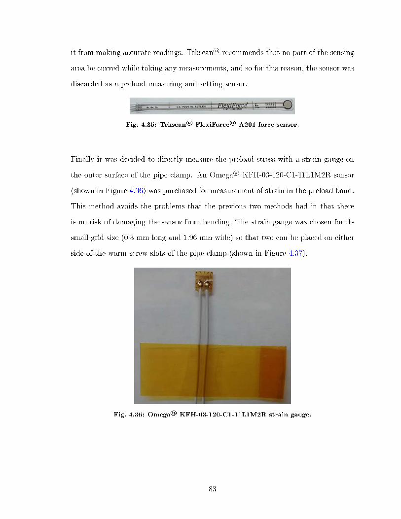
it from making accurate readings. Tekscan® recommends that no part of the sensing
area be curved while taking any measurements, and so for this reason, the sensor was
discarded as a preload measuring and setting sensor.
Fig. 4.35: Tekscan® FlexiForce® A201 force sensor.
Finally it was decided to directly measure the preload stress with a strain gauge on
the outer surface of the pipe clamp. An Omega® KFH-03-120-C1-11L1M2R sensor
(shown in Figure 4.36) was purchased for measurement of strain in the preload band.
This method avoids the problems that the previous two methods had in that there
is no risk of damaging the sensor from bending. The strain gauge was chosen for its
small grid size (0.3 mm long and 1.96 mm wide) so that two can be placed on either
side of the worm screw slots of the pipe clamp (shown in Figure 4.37).
Fig. 4.36: Omega® KFH-03-120-C1-11L1M2R strain gauge.
83

Fig. 4.37: Omega® strain gauge mounted on a preloaded transducer.
The previous model of solid transducers give an estimate of the upper bound of
the preload tension of 438.41 N2
= 219.21 N. 219.21 N is the preload tension which
minimizes the radial stress in the PZT at a load of 367.875 N, the estimated load
experienced by an individual transducer in a harvesting pad being loaded by a 1500 Kg
vehicle. The reason that the value is divided by 2 is to reduce the radial compressive
force applied by the preload tension, while allowing a tensile force to exist in the PZT
during compression. It is assumed that the peak compressive force, experienced by
the PZT while not loaded and the peak radial tension of the same PZT disc while
fully loaded will have approximately the same magnitude. To measure the strain in
the preload clamps, the cross section is needed. The areas where the strain gauges
are attached are measured to be 2.72 mm and 2.92 mm wide, and 0.50 mm thick,
and are calculated as being (0.00272 m + 0.00292 m) 0.0005 m = 2.82 × 10⁻⁶ m2.
The average stress can be calculated as 219.21 N2.82×10−6 m2 = 7.77 × 10⁷ Pa. Substituting
that value into Equation 4.2 and assuming that the stainless steel band has a similar
Young's modulus as 301 stainless steel, the estimated strain can be calculated as:
84

Yxy =x
X
X =7.77× 10⁷
1.93× 1011= 4.03× 10⁻⁴
120.4 Ω GF 1.51
X =
(ΔRg
Rg
)/GF
ΔRg = 1.51 · 4.03× 10−4 · 120.4 Ω = 0.0732 Ω.
Rg
1.5 3

Standard measurements using a Wheatstone bridge will replace on of the resistors in
the bridge with a potentiometer. The reason for this is to use the potentiometer to
ajust the circuit such that the measured output voltage is zero. This compensates for
small amounts of current leakage from the measurement device. Because of electrical
noise introduced to the measurements by the potentiometer used, it was left out and
the Wheatstone bridge was left calibrated. Instead the voltage across the center was
measured, and is calculated as:
Vout = Vin
[Rg + ∆Rg
Rg + ∆Rg +R2
− R4
R3 +R4
](4.4)
Vout = 3
[120.4732
120.4732 + 120.271− 100.0
100.0 + 100.0
]= 1.30 mV.
A Tektronix® DMM4050 digital multimeter was used to make voltage measurements
using the Wheatstone bridge. A Tektronix® PWS4305 power supply was used to
provide the 3 volts needed to the bridge circuit. Because the initial voltage across
the bridge would not be exactly zero because the bridge wasn't compensated for, the
preload was adjusted until the output voltage was equal to the sum of the initial
measured voltage before preloading and the calculated voltage in Equation 4.4. Fig-
ure 4.39 shows a transducer set to the desired preload value with two strain gauges
attached for strain verication.
86
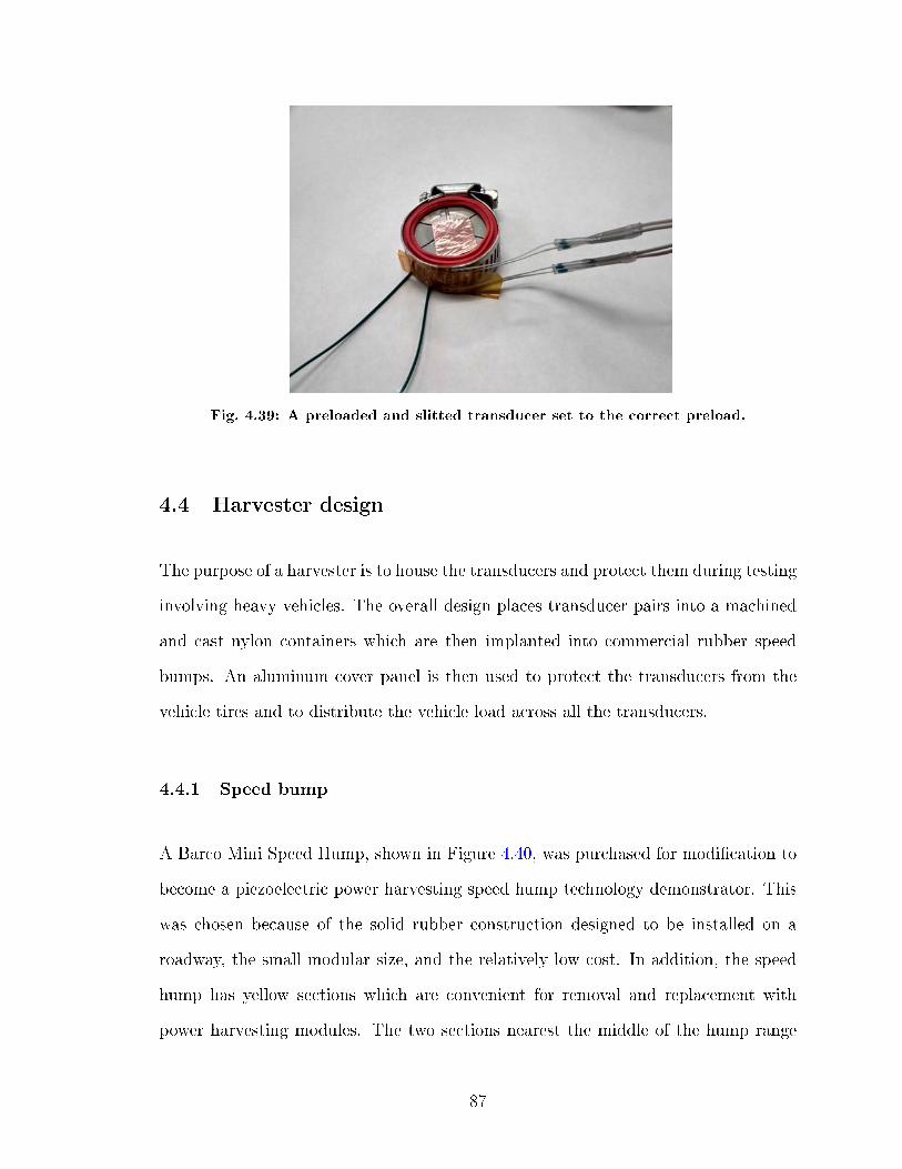
Fig. 4.39: A preloaded and slitted transducer set to the correct preload.
4.4 Harvester design
The purpose of a harvester is to house the transducers and protect them during testing
involving heavy vehicles. The overall design places transducer pairs into a machined
and cast nylon containers which are then implanted into commercial rubber speed
bumps. An aluminum cover panel is then used to protect the transducers from the
vehicle tires and to distribute the vehicle load across all the transducers.
4.4.1 Speed bump
A Barco Mini Speed Hump, shown in Figure 4.40, was purchased for modication to
become a piezoelectric power harvesting speed hump technology demonstrator. This
was chosen because of the solid rubber construction designed to be installed on a
roadway, the small modular size, and the relatively low cost. In addition, the speed
hump has yellow sections which are convenient for removal and replacement with
power harvesting modules. The two sections nearest the middle of the hump range
87

from 26 mm to 32 mm in thickness, sucient to allow room for the construction of
cast nylon transducer containers.
Fig. 4.40: Barco mini speed hump section.
4.4.2 Power harvesting module
The purpose for the power harvesting modules is to behave as a container to protect
the transducers it is housing from precipitation, dirt, and damage while acting as a
hard surface to press against the transducers. The housing is designed to accommo-
date transducers in vertical stacks, two transducers high to improve power generation.
Ten pockets are arranged in two rows of ve in order to accommodate ten transducer
pairs, or twenty individual transducers per harvesting module. Two types of power
harvesting modules were manufactured in order to house solid end capped transduc-
ers without preloading and the novel slitted and preloaded transducers. The two
sets of power harvesting units to be compared are housed in the specialized modules
shown in Figures 4.41 and 4.42, the former of which is designed for preloaded trans-
ducers, and the latter for the conventional units. Cast nylon was used and purchased
from McMaster-Carr® [48] due to its low cost, ease of machining, resistance to water
corrosion, rigidity, and dielectric properties.
88

3.70
9.50
.75
1.375
1.8751.75
.63
.10
.10
.12
.40
.50
R.13
All units in inches.Drawn by: Matteo Louter
SCALE 0.500
SCALE 0.500
Fig. 4.41: Power harvesting module design for accommodating preloaded trans-ducers.
3.70
9.50
.75
.301.15
.925
1.90
.34
.50
.10
.10
.12
SCALE 0.500
All units in inches.Drawn by: Matteo Louter
SCALE 0.500
Fig. 4.42: Power harvesting module design for standard cymbal transducers.
4.4.3 Manufacturing of preloaded transducers
The preloaded transducer end caps use a six slitted design cut using a water jet cutter
from 301 stainless steel. The two end caps in the bottom half of Figure 4.43 are shown
after water jet cutting and deburring is complete. The end caps in the top half of
Figure 4.43 are the result of punching the water cut discs into their nal shape using
the stamping setup shown in Figures 4.2 and 4.3. The slit FEA model determined
89

that 0.015 thick end cap is a suitable thickness, while the non slitted end caps used
the same 0.01 thick phosphor bronze as the earlier, successfully tested, transducers
did.
Fig. 4.43: Slitted end caps before and after stamping.
After the slitted end caps are punched into the desired cymbal shape, they are rough-
ened and cleaned to better adhere to the LePage® speed set professional epoxy and
to the PZT discs. Figure 4.44 shows the transducers during the curing process held
together with six binder clips (left) and at the end of the process with the binder
clips o (right). In addition to the conventional epoxy, small dots of MG Chemicals®
silver conductive epoxy were used in order to conduct the power harvested to the end
cap material where the wiring will be attached.
Fig. 4.44: Preloaded transducers being epoxied (left) and the hardened trans-ducers (right).
In order to improve power generation, transducers were paired and stacked to increase
90

the compression displacement and double the power generated for each transducer
stack in the housing. Figure 4.45 shows the transducer pairs electrically connected
to each other along with wiring (left) using electrically conductive tape and shows
the completed transducers with rubber buers and preloading clamps in the right
image. Transducers were paired such that their polled directions face each other.
This allowed the contact point between transducers to be conductive and generate a
positive potential when the pair is compressed on the top of the upper transducer. The
top of the upper transducer and bottom of the lower transducer are then connected
with conductive tape and represent the negative terminal of the transducer pair.
The preloading utilized three thick lobster claw elastic bands to reduce the stress
concentrations from the irregular pressure of the steel pipe clamp screw mechanism
being pressed against the PZT ceramic disc.
Fig. 4.45: Preloaded transducers being paired up and electrically connected(left) and the nished preloaded transducers (right).
The completed preloaded transducers are then placed inside their machined nylon
housing (shown in Figure 4.46). Each transducer pair is then wired to their own
DF04M Fairchild Semiconductor full wave bridge rectier rated for 400 V and 1.5 A
to handle high voltage and current spikes.
91

Fig. 4.46: Preloaded transducer housing after machining with inserted trans-ducers.
Figure 4.47 depicts a malfunctioning transducer with its aluminum spacers to help
it contact the container cover and container bottom so load it applied in the correct
location. The defect was caused by conductive tape used to electrically connect
the negative terminals of the transducer pair being too short for some harvesting
transducer pairs and prevented the transducers from remaining horizontal and parallel
when being compressed. Care was taken to prevent such manufacturing defects.
Finally 3.2 mm thick by 12.6 mm diameter aluminum discs (also shown in Figure
4.47) are machined to increase the thickness of the two transducers such that their
thickness is greater than the width of the pipe clamp. This is necessary to conduct
the vehicle load from the top cover, through the transducer pairs, to the ground.
92

Fig. 4.47: Under performing slitted transducer.
4.4.4 Solid transducers
It was primarily damage resistance that the 0.01 thick phosphor bronze end caps
were chosen over the 0.008 thick stainless steel end caps. The solid transducer nylon
housing was machined and is shown installed in the rubber speed bump in Figure
4.48. Also shown is the 0.25 thick aluminum cover plate to more evenly distribute
a vehicle load over the transducers as well as prevent the transducers from wear and
dirt from the vehicle tire. Figure 4.49 shows the solid transducers assembled and
installed in the housing unit. Similar to the preloaded transducers, solid transducers
are stacked in pairs, and each pair connected to its own voltage rectier. Electrical
tape is used to hold the wiring in channels machined in the nylon.
93

Fig. 4.48: Machined non preloaded transducer housing module sitting in thespeed bump.
Fig. 4.49: Fully assembled non preloaded harvester.
The Cymbal transducer end caps where roughened and cleaned to improve adhesion
and remove bronze powder that would interfere with the end cap epoxy interface.
4.4.5 Assembly of the harvesting speed bump
The two completed harvesting modules were inserted into the speed bump pockets
made by removing the two central yellow rubber sections (shown in Figure 4.50).
Holes bored in the side of the speed bump act as external cable routing for the har-
vesting modules. The transducer pairs were each attached to their own respective
DF04M FairchildSemiconductor bridge rectier rated for 400 V and 1.5 A, all con-
nected to a common pair of power bus lines shown leaving the speed hump on the
94

left side of Figure 4.50. The rectiers are chosen for their low cost, high voltage tol-
erances, and DIP package for ease of soldering. Finally, 0.25” thick aluminum cover
plates are placed on top of the harvesters, shown in the right image of Figure 4.50,
for protection and even loading of the transducer pairs.
Fig. 4.50: Harvesters inserted into speed bump.
4.5 Vehicle testing
In order to verify the applicability of the roadway power harvesting system, practi-
cal tests are required. Though some tests can be carried out on the hydraulic test
machine, many factors cannot be reproduced on it such as non centered loading and
the sharp compression from a vehicle moving at high speed. The test vehicles weight
was determined by using a gravel pit scale, used for weighing dump trucks and was
measured as 1, 800 kg. This type of vehicle scale has a low resolution of ±100 kg and
can not measure individual wheels or axles.
4.5.1 Initial vehicle test setup
The initial roadway power harvester was tested using a vehicle in a parking garage as
shown in Figure 4.51. The purpose of the location was to have access to a power out-
let to operate the Tektronix® DPO 2024B oscilloscope that was used for all testing
experiments as well as providing an environment free of precipitation and other harsh
95

weather conditions. A 2003 Subaru outback, station wagon with a total measured
vehicle mass of 1, 800 kg, with fuel and driver, was driven over the speed bump mul-
tiple times using the heavier front and lighter rear tire to examine power generation
using diering vehicle loads. The bump was oriented such that the solid transducer
harvesting pad would be compressed rst as the car traversed over the speed bump in
its forward direction, and the preloaded units would be compressed after. Tests were
performed to compare vehicle driving direction to see what eect the direction of a
traversing vehicle may have on the voltages generated. The vehicle was also driven at
various speeds to determine if and how much, speed correlated with power generation.
Finally the two harvesting pads were connected together to examine the voltage pro-
le that a harvesting circuit would experience. The test setup shown in Figure 4.51
involved the power modules being directly connected to the oscilloscope which was
connected to a wall outlet using an extension cord. The oscilloscope was connected
to a laptop to collect the raw data and to perform data analysis later on. Other tests
were performed, examining the performance of potential harvesting circuits, however
that work is outside the scope of this thesis and is not discussed here.
Fig. 4.51: Vehicle test setup.
96
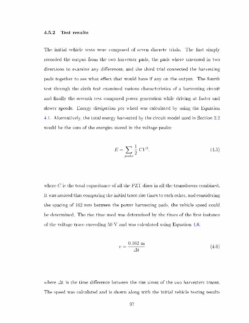
4.5.2 Test results
The initial vehicle tests were composed of seven discrete trials. The rst simply
recorded the output from the two harvester pads, the pads where traversed in two
directions to examine any dierences, and the third trial connected the harvesting
pads together to see what eect that would have if any on the output. The fourth
test through the sixth test examined various characteristics of a harvesting circuit
and nally the seventh test compared power generation while driving at faster and
slower speeds. Energy dissipation per wheel was calculated by using the Equation
4.1. Alternatively, the total energy harvested by the circuit model used in Section 2.2
would be the sum of the energies stored in the voltage peaks:
E =∑peaks
1
2CV 2. (4.5)
where C is the total capacitance of all the PZT discs in all the transducers combined.
It was noticed that comparing the initial trace rise times to each other, and considering
the spacing of 162 mm between the power harvesting pads, the vehicle speed could
be determined. The rise time used was determined by the times of the rst instance
of the voltage trace exceeding 50 V and was calculated using Equation 4.6.
v =0.162 m
∆t(4.6)
where ∆t is the time dierence between the rise times of the two harvesters traces.
The speed was calculated and is shown along with the initial vehicle testing results
97

shown in Table 4.6. The energy values in the column denoted Energy dissipated per
tire compression are calculated using Equation 4.1 and represent energy dissipated
through the oscilloscope. Test trials were conducted a single time making uncertainty
analysis dicult, however the uncertainty from the values in these tests can be esti-
mated from the uncertainty values measured and shown in Tables 4.1, 4.3, 4.4, and
4.5. It was possible to get an uncertainty estimation from trial 3 because several
compressions of the harvesting pads were done. In order to calculate the speed, the
traces of the separate harvesting pads must be kept separate. It is for this reason that
a vehicle speed could not be estimated for trial 3, as the inputs of the two harvesting
pads were combined.
Table 4.6: Initial vehicle test results.
Trial Averagespeedbetweenharvesting
pads
Harvester padEnergy
dissipated pertire compression
Peak voltagemeasured
1 2.19 Km
h
Solid 1.59 mJ 316 VSlitted andpreloaded
0.775 mJ 302 V
2 backward 3.34 Km
h
Solid 1.19 mJ 298 VSlitted andpreloaded
0.572 mJ 256 V
2 forward 3.04 Km
h
Solid 1.18 mJ 310 VSlitted andpreloaded
0.626 mJ 278 V
3 Combined 1.58 mJ 306− 296 V
7 slow 1.30 Km
h
Solid 2.07 mJ 288 VSlitted andpreloaded
1.43 mJ 304 V
7 fast 13.16 Km
h
Solid 0.223 mJ 344 VSlitted andpreloaded
0.286 mJ 450 V
The traces from the rst experiments shown in Figure 4.52 and Figure 4.53 depict
the raw voltage trace from both preloaded-slitted and solid transducers. The solid
98
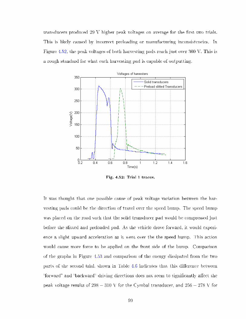
transducers produced 29 V higher peak voltages on average for the rst two trials.
This is likely caused by incorrect preloading or manufacturing inconsistencies. In
Figure 4.52, the peak voltages of both harvesting pads reach just over 300 V. This is
a rough standard for what each harvesting pad is capable of outputting.
Fig. 4.52: Trial 1 traces.
It was thought that one possible cause of peak voltage variation between the har-
vesting pads could be the direction of travel over the speed bump. The speed bump
was placed on the road such that the solid transducer pad would be compressed just
before the slitted and preloaded pad. As the vehicle drove forward, it would experi-
ence a slight upward acceleration as it went over the the speed hump. This action
would cause more force to be applied on the front side of the bump. Comparison
of the graphs in Figure 4.53 and comparison of the energy dissipated from the two
parts of the second trial, shown in Table 4.6 indicates that this dierence between
forward and backward driving directions does not seem to signicantly aect the
peak voltage results of 298− 310 V for the Cymbal transducer, and 256− 278 V for
99

the preloaded and slitted transducer. It is also noticed in Figure 4.53 that a secondary
voltage peak exists for the solid transducers. Because this peak is reversed with the
reversal of driving directions, it is likely caused by a structural component such as
the cover plate tilting while the vehicle load is applied across the covers surface.
Fig. 4.53: Trial 2 traces showing backward driving on the left, and forwarddriving on the right.
The third trial attempted to understand the eects of combining multiple harvesting
pads together to see if they would have a detrimental eect on each other or peak
voltage generation. The results for trial 3 shown in Figure 4.54 and numerically
in Table 4.6, show that the energy dissipated per tire compression, along with the
peak voltage, from trial 3 remained similar to the other tests at 306 − 296 V. The
average peak voltage of the other trials excluding trial 7 is 293.3 Vso the combined
pad voltage result is the result expected if they did not have an eect on one another
and represent a doubling of potential power to a harvesting circuit as per Equation
4.5. The disadvantage of connecting the terminals of both power harvesting pads, is
that speed determination is now more dicult to estimate and prone to more errors.
100

Fig. 4.54: Trial 3 traces.
Finally trial 7 tested to see if any dierences existed with the vehicle velocity, which
would cause the pulse width to shorten with higher velocities. The result from trial
7 appears to indicate that the peak output voltages for the slitted and preloaded
transducer are highly dependent on the traversing vehicle speed with the slitted and
preloaded transducer reaching the maximum measurement value of the oscilloscope
at 450 V. This apparent strong dependence on speed was unexpected and so further
exploration into this was performed. Figure 4.55 depicts the slitted and preloaded
transducer traces producing signicantly higher peak voltages than the solid trans-
ducers at a higher vehicle speed. This is potentially caused by larger forces and
deformations within the transducers, causing the more exible slitted transducers to
deform its PZT material further than the solid transducers are able to. The calcu-
lated speed is shown in the title of each graph in Figure 4.55 and is calculated by
dividing the spacing of the transducer pads by the dierence in measured rise times.
101

Fig. 4.55: Trial 7 traces showing voltage spikes corresponding to the heavierfront, and lighter rear tire loads.
Plotting all of the peak voltages for the tests, shown in Table 4.6, with their calculated
speed produces Figure 4.56. The slower speed experiments do not exhibit a correlation
with speed and peak voltage. The single higher speed test implies that, especially for
the preloaded and slitted transducer, that an increased speed will improve harvester
performance so this anomaly is explored in the following vehicle test.
Fig. 4.56: Summary of all the peak voltages of the August vehicle testing.
102
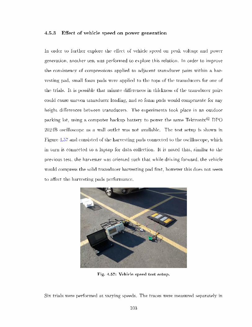
4.5.3 Eect of vehicle speed on power generation
In order to further explore the eect of vehicle speed on peak voltage and power
generation, another test was performed to explore this relation. In order to improve
the consistency of compressions applied to adjacent transducer pairs within a har-
vesting pad, small foam pads were applied to the tops of the transducers for one of
the trials. It is possible that minute dierences in thickness of the transducer pairs
could cause uneven transducer loading, and so foam pads would compensate for any
height dierences between transducers. The experiments took place in an outdoor
parking lot, using a computer backup battery to power the same Tektronix® DPO
2024B oscilloscope as a wall outlet was not available. The test setup is shown in
Figure 4.57 and consisted of the harvesting pads connected to the oscilloscope, which
in turn is connected to a laptop for data collection. It is noted that, similar to the
previous test, the harvester was oriented such that while driving forward, the vehicle
would compress the solid transducer harvesting pad rst, however this does not seem
to aect the harvesting pads performance.
Fig. 4.57: Vehicle speed test setup.
Six trials were performed at varying speeds. The traces were measured separately in
103
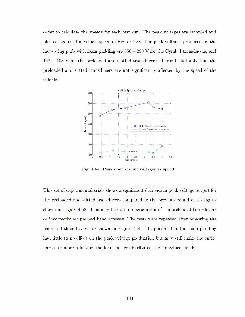
order to calculate the speeds for each test run. The peak voltages are recorded and
plotted against the vehicle speed in Figure 4.58. The peak voltages produced by the
harvesting pads with foam padding are 356− 290 V for the Cymbal transducers, and
142 − 108 V for the preloaded and slotted transducers. These tests imply that the
preloaded and slitted transducers are not signicantly aected by the speed of the
vehicle.
Fig. 4.58: Peak open circuit voltages vs speed.
This set of experimental trials shows a signicant decrease in peak voltage output for
the preloaded and slitted transducers compared to the previous round of testing as
shown in Figure 4.58. This may be due to degradation of the preloaded transducers
or incorrectly set preload band stresses. The tests were repeated after removing the
pads and their traces are shown in Figure 4.59. It appears that the foam padding
had little to no eect on the peak voltage production but may still make the entire
harvester more robust as the foam better distributed the transducer loads.
104

Fig. 4.59: Traces from the experimental transducers with foam padding re-moved.
Figure 4.60 also indicates that there is no correlation between speed and peak voltage
produced. This means that the earlier experimental ndings correlating speed to
voltage output are an anomaly. The peak voltages produced by the harvesting pads
without foam padding are 320− 310 V for the Cymbal transducers, and 128− 94 V
for the preloaded and slotted transducers. This could be caused by too much preload
tension applied to the slitted cymbal units and so this is explored in the following
test.
105

Fig. 4.60: Peak open circuit voltages vs speed with foam padding removed.
Comparison between the foam and no foam results indicate that the foam padding
did have a small positive eect on transducer performance, on average improving
the output by 16 V. This foam padding is added to the nal prototype due to its
potential benets.
4.5.4 Reducing preload tension
Since external environments where power harvesting would be implemented experi-
ence precipitation, there became a need to make the harvesting pads water resistant.
The harvesting pads were encased in large Ziploc® bags with only a small opening
for the power wires as shown in Figure 4.61.
106

Fig. 4.61: Waterproofed harvesting pads.
The transducers were also disassembled and their electrical connections reinforced
with additional conductive epoxy, as some connections could have been degrading.
Other transducers had begun shifting from the horizontal stacked conguration simi-
lar to the shifting seen in Figure 4.47 and were repaired. The heights of the transducer
pairs were checked and found to have been varying by measurable amounts, perhaps
causing some transducers to be loaded much more than others. Stainless steel discs,
0.008 (0.2032 mm) thick, were cut and stacked under the transducers to set them all
at approximately the same height ±0.1016 mm, to bring their average height above
the harvesting container to 1 mm. Finally, the preload tension was reduced for all
transducers to potentially increase their output power. Four experimental trials of
diering speed runs were undertaken and oscilloscope traces taken shown in Figure
4.62 and numerical results shown in Table 4.7. The trials were named V1, V2,
V3, and, V4 in order from slowest vehicle movement speed to fastest.
107

Fig. 4.62: Reduced preload traces.
Table 4.7: Peak voltage attained by transducers using reduced preloading ten-sion.
Trial Average speed Harvester pad Peak voltage measured
1 V1 5.63 Kmh
Solid 247 VSlitted and preloaded 304 V
2 V2 6.46 Kmh
Solid 268 VSlitted and preloaded 454 V
3 V3 11.6 Kmh
Solid 270 VSlitted and preloaded 454 V
4 V4 17.3 Kmh
Solid 282 VSlitted and preloaded 454 V
The results show the solid and preloaded transducers far out performing their solid
endcapped counterparts, with 454− 304 V compared to the 282− 247 V peaks from
the cymbal transducers. Small voltage spikes, separate from the main spikes in traces
V1, V3, and V4 indicate that the transducers are experiencing damage. After
20 to 30 more vehicle compressions were performed, for the testing of a harvesting
circuit, a nal open circuit test was completed shown in Figure 4.63. There appears
to be slightly reduced peak voltage from both harvesting pads in this last degradation
108
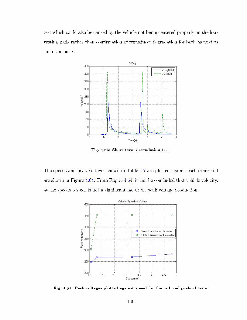
test which could also be caused by the vehicle not being centered properly on the har-
vesting pads rather than conrmation of transducer degradation for both harvesters
simultaneously.
Fig. 4.63: Short term degradation test.
The speeds and peak voltages shown in Table 4.7 are plotted against each other and
are shown in Figure 4.64. From Figure 4.64, it can be concluded that vehicle velocity,
at the speeds tested, is not a signicant factor on peak voltage production.
Fig. 4.64: Peak voltages plotted against speed for the reduced preload tests.
109

It now appears that the power production is much higher for the slitted preloaded
transducers as their peak voltages are consistently higher at all speeds. Three of the
four tests returned a peak voltage value of 454 V which seems to be the peak voltage
that the oscilloscope can measure. The oscilloscope itself is rated to 400 V. Given the
oscilloscope measurement limitations and the identical peak voltages shown in Figure
4.64, it seems likely that the measured voltages have been truncated to 454 V. It
should also be noted that the bridge rectiers connecting the transducer pairs to the
main output wires are rated for a maximum reverse voltage of 400 V necessitating an
upgrade for the bridge rectiers.
4.5.5 Transducer damage
It was noticed after the reduced preload tension tests that some of the traces collected
such as Figures 4.62 and 4.63, showed odd voltage spikes after the main vehicle com-
pression and release. This behavior was seen before in earlier tests as seen in Figure
4.55 but was ignored as anomalous noise. Qualitatively examining transducers and
their traces, it was found that some pairs produced jagged traces which corresponded
to apparent cracks in the PZT material. Some examples of damaged transducer traces
are shown in Figure 4.65 and an example of a damaged transducer is shown in Fig-
ure 4.66. The traces were produced by nding transducers with apparent cracks and
manually applying a force to the unit to examine the trace.
110

Fig. 4.65: Damaged transducer traces.
Fig. 4.66: Damaged transducer in a pair.
The damaged transducers were taken apart for examination and the piezo disc from
the damaged transducer shown in Figure 4.66 is shown in Figure 4.67. In order to
continue testing, three transducers were taken apart and replaced with new ones as
there was only enough leftover piezo material to allow for three more replacement
units to be manufactured.
111

Fig. 4.67: Damaged piezo disc from Figure 4.66.
Fig. 4.68: The second damaged transducer disassembled.
The three transducers to be replaced were ones that showed the highest amount of
cracking damage around the outside edge. The second of the three transducers taken
apart had damage similar or exactly to that of Figure 4.67 shown in Figure 4.68, while
the third piezo transducer suered much deeper cracking which appeared to associate
with the slitted end caps discrete contact areas and is shown in Figure 4.69. These
damage patterns, which seem to follow and be caused by the slitted end caps, appear
very dierent from other damage tests performed on the MTS® machine using solid
transducers were there was a tendency of piezo units to shatter or crack through the
center.
Fig. 4.69: The most heavily damaged piezo unit examined.
112

The damaged transducers are still be capable of generating signicant voltages due
to the relaxation of their preloading when a vehicle load is applied to the transducer
pair however their potential is lowered as they cannot generate power from tension.
While unloaded, the damaged transducers will be under compressive loading from
their preloading bands. The relaxation of this compressive loading from the external
transducer loading would still cause the PZT fragments to generate a proportional
electric eld, thereby producing electricity. This mechanism could only work up to
the point when the radial stress changes sign from compressive to tensile, in which
case the PZT fragments would separate and no more power would be generated.
4.6 Full scale roadway harvester
In order to demonstrate the roadway power harvesting system, a full scale roadway
power harvester was designed and constructed.
4.6.1 Full scale harvester design and fabrication
The updated system uses two speed bumps, with four harvesting pads in each for a
total of eight harvesting pads. The nylon container design was modied to allow built
in spacers at the bottom of the individual cells to make contact with each transducer.
Holes for the bridge rectiers where also moved in a more convenient location on the
harvesting pad and enlarged, which are shown in Figure 4.70. The harvesting pad was
machined on a Computer Numeric Control (CNC) machine and as such was designed
using the parameters (shown in Figure 4.70) which are dened in inches.
113

3.70
9.50
.75
.925
1.8751.75
R.6875
R1/8
.43.63
.10
.12
.50
.12
All units in inches.Drawn by: Matteo Louter
SCALE 0.500
Fig. 4.70: Improved harvesting pad housing design.
The design called for eight harvesting pads with ten transducer pairs each totaling
80 transducer pairs or 160 individual transducers which were hand assembled using
methods previously described and are shown in partial assembly in Figure 4.71.
(a) All 80 transducers paired oand under assembly.
(b) Transducer pairs assembled,preloaded, and placed in thenylon housings.
Fig. 4.71: Transducers at various stages of assembly.
The cover panels for the harvesting pads were covered in black and yellow anti-slip
114
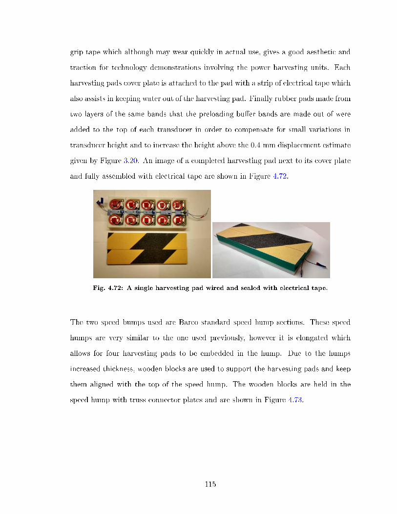
grip tape which although may wear quickly in actual use, gives a good aesthetic and
traction for technology demonstrations involving the power harvesting units. Each
harvesting pads cover plate is attached to the pad with a strip of electrical tape which
also assists in keeping water out of the harvesting pad. Finally rubber pads made from
two layers of the same bands that the preloading buer bands are made out of were
added to the top of each transducer in order to compensate for small variations in
transducer height and to increase the height above the 0.4 mm displacement estimate
given by Figure 3.20. An image of a completed harvesting pad next to its cover plate
and fully assembled with electrical tape are shown in Figure 4.72.
Fig. 4.72: A single harvesting pad wired and sealed with electrical tape.
The two speed bumps used are Barco standard speed hump sections. These speed
humps are very similar to the one used previously, however it is elongated which
allows for four harvesting pads to be embedded in the hump. Due to the humps
increased thickness, wooden blocks are used to support the harvesting pads and keep
them aligned with the top of the speed hump. The wooden blocks are held in the
speed hump with truss connector plates and are shown in Figure 4.73.
115

Fig. 4.73: Speed bump with truss connector plates used to attach the woodenspacers.
Figure 4.74 shows one of the two speed humps before and after installation of the
harvesting pads. Holes were drilled into the sides of the speed humps to route the
cables which carry the harvested power to a power conditioning circuit.
Fig. 4.74: Harvesting pads on top of and placed in the speed bump.
116

4.6.2 Full scale harvester test
The test setup was similar to those of previous tests and used one of the two harvesting
pads as they have been constructed identically. An extension cable was used to power
the Tektronix® DPO 2024B oscilloscope and a laptop used to record the trace data.
Figure 4.75 shows the testing setup with the test vehicle, the same one used on
all other tests, barely visible in the top right corner of the image. For referencing
purposes, the harvesting pads were given numerical designations 1 - 4 from left to
right as shown in in both Figure 4.74 and 4.75.
Fig. 4.75: Full scale harvester test setup.
An initial test was performed with all harvesting pads, except harvesting pad 2,
removed. The resulting trace taken is shown in Figure 4.76. The peak voltage exceeds
the oscilloscopes ability to measure it and far exceeds the voltage probes peak rated
voltage of 300 V.
117
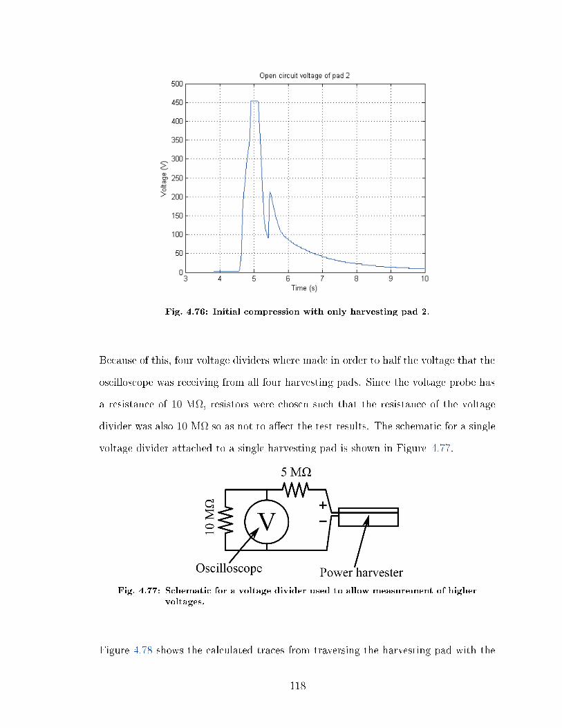
10 Ω
10 Ω

front wheel of the same vehicle used in all tests. The recorded traces were simply
doubled to extrapolate the actual voltages produced by the harvesting pads.
Fig. 4.78: Calculated full scale traces from initial front wheel loading.
Seven, 20 pound weights where added incrementally to the vehicle up to 140 pounds,
between the rear wheels to examine the eect that vehicle weight would have on the
harvesting pads output. Figure 4.79 shows the placement of the weights in the test
vehicle.
119

Fig. 4.79: All seven, 20 lb weights placed in the rear of the test vehicle.
The results from the rear wheel loading tests reveal several points. Figure 4.80a
and 4.80b show the extrapolated voltage traces for rear wheel loading at 0 and 20
additional pounds. It can be seen that the peak voltages change in a way that indicates
that the driving direction plays a signicant role in the peak voltage production.
Furthermore by comparing a loading scenario using the heavier front wheel (shown in
Figure 4.78) to the rear wheel with no additional load (shown in Figure 4.80a) it can
be seen that very similar peak voltages are produced, indicating that the transducers
are compressed fully and additional loading force is being absorbed by the transducers
protective housing. The vehicle loading in the two scenarios mentioned previously are
applied with the vehicle traveling in the same direction further indicating that weight
has little eect and that loading direction has a much more signicant eect.
120

(a) Calculated voltage trace with 0 poundwheel loading.
(b) Calculated voltage trace with 20pound wheel loading.
Fig. 4.80: Calculated voltage traces for rear wheel loading scenarios.
Figure 4.81 plots the calculated peak voltages over the ranges of additional loading's
tested and shows no signicant or consistent change caused by increased weight.
Comparing the two sub gures together however (Figure 4.81a and 4.81b) shows a
large dierence caused by the direction the vehicle traversed the harvesting pads.
This may be caused by the harvesting pads protruding from the speed bump at their
edges, a phenomenon caused by the horizontal mounting of the pads, and the speed
bumps curved driving surface.
(a) Calculated peak voltages for vehiclemotion from pad 1 to pad 4.
(b) Calculated peak voltages for vehiclemotion from pad 4 to pad 1.
Fig. 4.81: Calculated peak voltages from all harvesting pads plotted against theadded mass for rear wheel loading scenarios.
121

Finally, measurements where taken at various vehicle speeds to examine the eect
speed may have on the new full scale harvester. Figure 4.82 plots the average peak
pad voltage against the speed measured by comparing voltage rise times and knowing
the pad separation distance. From this test, it does not appear that speed signicantly
aects the power harvesters output.
Fig. 4.82: Vehicle speed vs average peak harvesting pad voltage.
Using Equation 2.2 and the average peak voltages displayed in Figure 4.81, the total
possible energy per tire compression can be calculated as:
1
2CtotalV
2avg =
1
2· 6.33× 10−7 H · 584 V = 0.108 J.
Assuming a daily trac value of 150,000, each vehicle having a single front and rear
tire, the single harvesting pad is calculated to, on average, continuously output:
300, 0001
day· 0.108 J
(1
24
day
h
)(1
60
h
min
)(1
60
min
s
)= 0.375 W.
122

And with both pads operating together, an average ideal output would be 0.751 W.
This value is much higher than the estimation made at the end of Chapter 2 due to
the much higher than expected peak voltages, however inevitable ineciencies in any
harvesting circuitry would reduce the usable power output.
This experiment demonstrates the improved power production capabilities of radi-
ally slitted and preloaded piezoelectric cymbal transducers applied to roadway power
harvesting. Peak voltages recorded for the solid, non slitted and non preloaded trans-
ducers were 344 V less than the peak voltage from the novel transducer design at
732 V. This represents a 113 % increase in peak voltage production indicating that
preloading and radially slitted designs may be the next way forward in roadway power
harvesting.
123

5 Conclusion
5.1 Summary
Cymbal transducers continue to be a viable option for roadway power harvesting due
to their simplicity, ease of manufacture and lack of actuating joints. This thesis has
demonstrated design and construction of a radially slitted and preloaded transducer,
designed for roadway power harvesting applications. The transducers are bundled into
a power harvesting speed bump system capable of generating and storing electricity
by way of vehicles compressing the bump. The system is then capable of delivering the
stored energy via a power conditioning circuit to an arbitrary application at a specied
voltage. By applying a radial compressive preload we are able to improve the damage
resistance of standard Cymbal piezoelectric transducers. This compensates for the
increased radial tensile loading of higher compressive loading situations. Combined
with a radially slitted Cymbal end cap design, the new transducer can output up
to 732 V which is 113 % more power than a conventional cymbal design. These new
transducers, though larger and more complex to manufacture, are specically designed
for high load and higher power applications. These improvements also reduce the
number of transducers needed for a specic application as the transducers that do
exist apply a larger range of strain to their piezoelectric materials and can generate
more power.
In addition it was found that by examining voltage rise times between sequential
harvesting pads, the vehicles speed could be measured. Further exploration of this
ability could lead to automated vehicle speed monitoring which wouldn't require
additional roadway sensors and be an added feature to any roadway power harvesting
system. Addition of a speed monitoring feature would require additional circuitry
though such circuitry could be integrated into the existing PCB so that the compact
124

nature of the integrated circuit board could be maintained.
5.2 Recommendations for future work
Improvements to the mechanical design of the roadway power harvesting transducers
are as follows. Improvements could be made to manufacturing quality, by improv-
ing the type and thickness of the buer rubber applied between the transducer and
preload band. The preload band itself can be improved by designing a mechanism to
allow the band to expand and contract with the transducer while applying a specic
and continuous preload force. This improvement would also assist in estimating and
setting a desired preload tension without need for strain gauges.
Improvements to the hardware prototypes include improvements to the securing
method when installing pads in the rubber speed bump and improvements in terms
of more weather resistant and waterproof harvesting container sealing. In addition,
custom speed bumps could be designed to maximize the number of harvesting pads
that they could accept. Methods for implanting the roadway harvesting pads into the
road surface also still needs to be addressed including installation and wiring methods.
Finally the design of the housing can be further improved by exploring more ecient
transducer pattern layouts and tailoring layout shapes to specic applications and
consumer needs.
Final improvements to the parametric design can be made by discarding assumptions
made about the independence of parameters on each other and their aect on per-
formance. Black box global optimization such as Kriging can be used in order to ne
tune the basic transducer parameters for more specialized applications using FEA
models.
Manufacturing processes can also be improved by exploring cheaper methods of cut-
125

ting the end cap shapes such as machining or combining punching and cutting which
may drastically lower cost especially if producing large batches of transducers. Fi-
nally the assembly of the transducers can be improved by using a more uniform and
consistent epoxy application method such as spin coating as used in [44], and nding
a more consistent way of applying the silver conductive epoxy.
126

References
[1] D. Hill, A. Agarwal, and N. Tong, Assessment of Piezoelectric Materials ForRoadway Energy: Cost of Energy and Demonstration Roadmap, DNV KEMAEnergy & Sustainability, Tech. Rep., 2014.
[2] S. R. Anton and H. a. Sodano, A review of power harvesting using piezoelectricmaterials (2003-2006), Smart Materials and Structures, vol. 16, no. 3, pp.R1R21, Jun. 2007. [Online]. Available: http://stacks.iop.org/0964-1726/16/i=3/a=R01?key=crossref.2c5609f4e60f2ce4b89d0db98aedfe93
[3] C.-C. Ting, D.-Y. Tsai, and C.-C. Hsiao, Developing a mechanical roadwaysystem for waste energy capture of vehicles and electric generation,Applied Energy, vol. 92, pp. 18, Apr. 2012. [Online]. Available: http://linkinghub.elsevier.com/retrieve/pii/S0306261911006556
[4] H. Zhao, J. Yu, and J. Ling, Finite element analysis of Cymbal piezoelectrictransducers for harvesting energy from asphalt pavement, Journal of theCeramic Society of Japan, vol. 118, no. 1382, pp. 909915, 2010. [Online].Available: http://joi.jlc.jst.go.jp/JST.JSTAGE/jcersj2/118.909?from=CrossRef
[5] P. Kemball-Cook, L. and Tucker, Energy harvesting, 2013. [Online]. Available:https://www.google.com/patents/US20130068047
[6] H. Abramovich, C. Milgrom, E. Harash, L. E. Azulay, and U. Amit, Multi-LyerPiezoelectric Generator, 2012.
[7] H. Abramovich, E. Harash, C. Milgrom, and U. Amit, Energy Harvesting FromAirport Runway, 2009.
[8] H. Abramovich, E. Harash, C. Milgrom, U. Amit, and L. E. Azulay, PowerHarvesting From Railway Aapparatus, System And Method, 2010.
[9] M. S. Vijaya, Piezoelectric Materials and Devices Applications in Engineeringand Medical Sciences. Taylor & Francis, 2012.
[10] J. F. Tressler, W. C. K. Uchino, and R. E. Newnham, Finite element analysisof the cymbal-type extensional transducer, IEEE Transactions on Ultrasonics,Ferroelectrics, and Frequency Control, vol. 45, no. 5, pp. 13631369, 1998.
[11] V. Piefort, Finite Element Modelling of Piezoelectric Active Structures, Ph.D.dissertation, Université Libre de Bruxelles, 2001.
[12] R. J. Meyer, W. J. Hughes, T. C. Montgomery, D. C. Markley, and R. E. Newn-ham, Design of and Fabrication Improvements to the Cymbal Transducer Aidedby Finite Element Analysis, Journal of Electroceramics, vol. 8, pp. 163 174,2002.
127
[13] S. Lin, An improved cymbal transducer with combined piezoelectric ceramicring and metal ring, Sensors and Actuators, A: Physical, vol. 163, no. 1, pp.266276, 2010. [Online]. Available: http://dx.doi.org/10.1016/j.sna.2010.06.022
[14] Z. Jindong, W. J. Hughes, A.C. Hladky-Hennion, and R. E. Newnham, Concavecymbal transducers, in Innovations in Materials Conference, Washington, D.C.,1999, pp. 252255.
[15] F. Bejarano, A. Feeney, and M. Lucas, A cymbal transducer forpower ultrasonics applications, Sensors and Actuators A: Physical, vol.210, no. April, pp. 182189, Apr. 2014. [Online]. Available: http://linkinghub.elsevier.com/retrieve/pii/S0924424714000880
[16] M. Nouh, O. Aldraihem, and a. Baz, Energy Harvesting ofThermoacoustic-Piezo Systems With a Dynamic Magnier, Journal ofVibration and Acoustics, vol. 134, no. 6, p. 061015, Oct. 2012.[Online]. Available: http://vibrationacoustics.asmedigitalcollection.asme.org/article.aspx?doi=10.1115/1.4005834
[17] R. Murray and J. Rastegar, Novel Two-Stage Piezoelectric-Based Ocean WaveEnergy Harvesters for Moored or Unmoored Buoys, Active and Passive SmartStructures and Integrated Systems, vol. 7288, pp. 72 880E72 880E12, Mar.2009. [Online]. Available: http://proceedings.spiedigitallibrary.org/proceeding.aspx?articleid=821922
[18] N. S. Shenck, A Demonstration of Useful Electric Energy Generationfrom Piezoceramics in a Shoe, Ph.D. dissertation, Massachusetts Instituteof Technology, 1997. [Online]. Available: http://resenv.media.mit.edu/pubs/theses/Nate-Thesis-Final.PDF
[19] J. Palosaari, M. Leinonen, J. Hannu, J. Juuti, and H. Jantunen, Energyharvesting with a cymbal type piezoelectric transducer from low frequencycompression, Journal of Electroceramics, vol. 28, no. 4, pp. 214219, Mar.2012. [Online]. Available: http://link.springer.com/10.1007/s10832-012-9713-8
[20] S. Priya and D. J. Inman, Energy harvesting technologies. Springer, 2008.
[21] J. Kymissis, C. Kendall, J. Paradiso, and N. Gershenfeld, Parasitic power har-vesting in shoes, Digest of Papers. Second International Symposium on WearableComputers (Cat. No.98EX215), 1998.
[22] A. Pirisi, F. Grimaccia, M. Mussetta, and R. Zich, Novel Speed BumpsDesign and Optimization for Vehicles' Energy Recovery in Smart Cities,Energies, vol. 5, no. 12, pp. 46244642, Nov. 2012. [Online]. Available:http://www.mdpi.com/1996-1073/5/11/4624/
[23] D. Arnold, W. Kinsel, W. W. Clark, and C. Mo, Exploration of NewCymbal Design in Energy Harvesting, Active and Passive Smart Structures
128

and Integrated Systems, vol. 7977, pp. 16, 2011. [Online]. Available:http://proceedings.spiedigitallibrary.org/proceeding.aspx?articleid=729212
[24] Y. Jiangbo, S. Xiaobiao, X. Tao, and C. Weishan, Modeling and Improvementof a Cymbal Transducer in Energy Harvesting, Journal of Intelligent MaterialSystems and Structures, vol. 21, no. 8, pp. 765771, Mar. 2010. [Online].Available: http://jim.sagepub.com/cgi/doi/10.1177/1045389X10366318
[25] C. Mo, D. Arnold, W. C. Kinsel, and W. W. Clark, Modelingand experimental validation of unimorph piezoelectric cymbal design inenergy harvesting, Journal of Intelligent Material Systems and Structures,vol. 24, no. 7, pp. 828836, Nov. 2012. [Online]. Available: http://jim.sagepub.com/cgi/doi/10.1177/1045389X12463459
[26] T. Purviance, S. Wickler, K. Clayson, T. Barnes, and C. Mo, Development oflow-prole piezoelectric energy harvester for high load application, in Technolo-gies for Sustainability (SusTech), 2013 1st IEEE Conference on. IEEE, 2013,pp. 120125.
[27] P. Materials, Piezoelectric materials, Electronics and Power, vol. 21, p. 53,1975.
[28] Ltd Apc International, Piezoelectric Ceramics. Mackyville: American PiezoCeramis International, 2011.
[29] R. Ballas, G., Piezoelectric Multilayer Beam Bending Actuators: Static and Dy-namic Behavior and Aspects of Sensor Integration. Springer London, Limited,2007.
[30] J. W. Morris, Notes on the Thermodynamics of Solids Chapter 15 : Tensors andTensor Properties, pp. 274328, 2008. [Online]. Available: http://www.mse.berkeley.edu/groups/morris/MSE201/Lecture_Notes/15.tensorproperties.pdf
[31] Noliac Group, Noliac Ceramics NCE datasheet, p. 12. [Online]. Avail-able: http://www.noliac.com/Files/Billeder/02Standard/Ceramics/Noliac_CEramics_NCE_datasheet.pdf
[32] C. Benham, P.P. and Crawford, R.J. and Armstrong, Mechanics of EngineeringMaterials. Longman Group, 1996.
[33] J. Dicken, P. D. Mitcheson, I. Stoianov, and E. M. Yeatman, Power-extractioncircuits for piezoelectric energy harvesters in miniature and low-power applica-tions, IEEE Transactions on Power Electronics, vol. 27, pp. 45144529, 2012.
[34] G. D. Szarka, B. H. Stark, and S. G. Burrow, Review of power conditioning forkinetic energy harvesting systems, IEEE Transactions on Power Electronics,vol. 27, no. 2, pp. 803815, 2012.
129

[35] E. A. Grace, S. E. Rajan, and A. C. Asis, Performance evaluation ofdierent rectiers for Piezo-electric energy harvesting applications, 2011International Conference on Recent Advancements in Electrical, Electronicsand Control Engineering, pp. 248252, Dec. 2011. [Online]. Available:http://ieeexplore.ieee.org/lpdocs/epic03/wrapper.htm?arnumber=6129810
[36] E. Lefeuvre, Piezoelectric Energy Harvesting Device Optimization bySynchronous Electric Charge Extraction, Journal of Intelligent MaterialSystems and Structures, vol. 16, no. 10, pp. 865876, Oct. 2005. [Online].Available: http://jim.sagepub.com/cgi/doi/10.1177/1045389X05056859
[37] a. Badel, Eciency Enhancement of a Piezoelectric Energy Harvesting Devicein Pulsed Operation by Synchronous Charge Inversion, Journal of IntelligentMaterial Systems and Structures, vol. 16, no. 10, pp. 889901, Oct. 2005. [Online].Available: http://jim.sagepub.com/cgi/doi/10.1177/1045389X05053150
[38] H. Zhao, J. Ling, and J. Yu, A comparative analysis of piezoelectric transducersfor harvesting energy from asphalt pavement, Journal of the Ceramic Societyof Japan, vol. 120, pp. 317323, 2012.
[39] Ministry of Transportation, Provincial Highways Trac Volumes2010, Tech. Rep., 2010. [Online]. Available: http://www.raqsb.mto.gov.on.ca/techpubs/TracVolumes.nsf/fa027808647879788525708a004b5df8/f51986ea499a13b08525745f006dd30b/\protect\T1\textdollarFILE/ProvincialHighwaysTracVolumes2010AADTOnly.pdf
[40] MicroStrain, Powering an EH-Link with piezoelectric source, p. 12, 2011.[Online]. Available: http://les.microstrain.com/tech_notes/PZT_TN_Rev0.2.pdf
[41] A. Dogan, Flextensional" moonie and Cymbal" Actuators, Ph.D. dissertation,Pennsylvania State University., 1994.
[42] A. Dogan and E. Uzgur, Size and Material Eects on Cymbal Transducerfor Actuator Applications, Ferroelectrics, vol. 331, no. 1, pp. 5363,Mar. 2006. [Online]. Available: http://www.tandfonline.com/doi/abs/10.1080/00150190600734955
[43] Y. Ke, T. Guo, and J. Li, A new-style, slotted-cymbal transducer with largedisplacement and high energy transmission, IEEE Transactions on Ultrasonics,Ferroelectrics, and Frequency Control, vol. 51, no. 9, pp. 11711177, 2004.
[44] M. Narayanan and R. W. Schwartz, Design, fabrication and nite elementmodeling of a new wagon wheel extensional transducer, Journal ofElectroceramics, vol. 24, no. 3, pp. 205213, Dec. 2008. [Online]. Available:http://link.springer.com/10.1007/s10832-008-9559-2
130

[45] F. Wolf, a. Sutor, S. J. Rupitsch, and R. Lerch, Modeling and measurementof inuence of mechanical prestress on hysteresis of ferroelectric actuators,Procedia Engineering, vol. 25, pp. 16131616, 2011. [Online]. Available:http://dx.doi.org/10.1016/j.proeng.2011.12.399
[46] H. W. Kim, S. Priya, K. Uchino, and R. E. Newnham, Piezoelectric energyharvesting under high pre-stressed cyclic vibrations, Journal of Electroceramics,vol. 15, pp. 2734, 2005.
[47] A. Badel, A. Benayad, E. Lefeuvre, L. Lebrun, C. Richard, and D. Guyomar,Single crystals and nonlinear process for outstanding vibration-powered electri-cal generators, IEEE Transactions on Ultrasonics, Ferroelectrics, and FrequencyControl, vol. 53, no. 4, pp. 673683, 2006.
[48] McMaster-Carr, More About Stainless Steel Alloys, p. 2, 2010. [Online].Available: http://www.mcmaster.com/
[49] K. Uchino, Ferroelectric Devices, J. Giniewicz, Ed. New York, Basel, HongKong: CRC Press, 2000.
[50] N. Putthongchai, T. Kulworawanichpong, P. Laoratanakul, and S. Srilomsak,Eects of Composition and Diameter of PZT Transducers on EnergyHarvesting, Integrated Ferroelectrics, vol. 114, no. 1, pp. 8191, Nov. 2010.[Online]. Available: http://www.tandfonline.com/doi/abs/10.1080/10584587.2010.488604
[51] Fujilm, Prescale, 2015. [Online]. Available: http://www.fujilm.com/products/prescale/prescalelm/#See_All
131