novel quantum phase transitions in low-dimensional systems
TRANSCRIPT
Novel Quantum Phase Transitions in
Low-Dimensional Systems
A dissertation presented
by
Junhyun Lee
to
The Department of Physics
in partial fulfillment of the requirements
for the degree of
Doctor of Philosophy
in the subject of
Physics
Harvard University
Cambridge, Massachusetts
April 2016

c�2016 Junhyun Lee
All rights reserved.
Dissertation advisor Author
Subir Sachdev Junhyun Lee
Novel Quantum Phase Transitions in Low-Dimensional
Systems
Abstract
We study a number of quantum phase transitions, which are exotic in their na-
ture and separates non-trivial phases of matter. Since quantum fluctuations, which
drive these phase transitions, are stronger in low-dimensions, we concentrate on low-
dimensional systems. We consider two di↵erent two-dimensional systems in this thesis
and study their phase transition.
First, we investigate a phase transition in graphene, one of the most famous two-
dimensional systems in condensed matter. For a suspended bilayer graphene in ⌫ = 0
quantum Hall regime, the conductivity data and mean-field analysis suggests a phase
transition from an antiferromagnetic (AF) state to a valence bond solid (VBS) state,
when perpendicular electric field is increased. This AF to VBS phase transition is
reminiscent of deconfined criticality, which is a novel phase transition that cannot
be explained by Landau’s theory of symmetry breaking. We show that in the strong
coupling regime of bilayer graphene, the AF state is destabilized by the transverse
electric field, likely resulting in a VBS state. We also consider monolayer and bilayer
graphene in the large cyclotron gap limit and show that the e↵ective action for the AF
and VBS order parameters have a topological Wess-Zumino-Witten term, supporting
that the phase transition observed in experiments is in the deconfined criticality class.
Second, we study the model systems of cuprate superconductor, which is e↵ec-
tively a two-dimensionalal system in the CuO2 plane. The proposal that the pseu-
dogap metal is a fractionalized Fermi liquid described by a quantum dimer model
is extended using the density matrix renormalization group. Measuring the Friedel
oscillations in the open boundaries reveals that the fermionic dimers have dispersion
minima near (⇡/2, ⇡/2), which is compatible with the Fermi arcs in photoemission.
iii
Abstract
Moreover, investigating the entanglement entropy suggests that the dimer model with
low fermion density is similar to the free fermion system above the Lifshitz transi-
tion. We also study the phase transition from a metal with SU(2) spin symmetry
to an AF metal. By applying the functional renormalization group to the two-band
spin-fermion model, we establish the existence of a strongly coupled fixed point and
calculate critical exponents of the fixed point.
iv
Contents
Title Page . . . . . . . . . . . . . . . . . . . . . . . . . . . . . . . . . . . . iAbstract . . . . . . . . . . . . . . . . . . . . . . . . . . . . . . . . . . . . . iiiTable of Contents . . . . . . . . . . . . . . . . . . . . . . . . . . . . . . . . vCitations to Previously Published Work . . . . . . . . . . . . . . . . . . . viiAcknowledgments . . . . . . . . . . . . . . . . . . . . . . . . . . . . . . . . viiiDedication . . . . . . . . . . . . . . . . . . . . . . . . . . . . . . . . . . . . x
1 Introduction 11.1 Electronic properties of graphene . . . . . . . . . . . . . . . . . . . . 31.2 Deconfined criticality . . . . . . . . . . . . . . . . . . . . . . . . . . . 71.3 Numerical methods in strongly correlated systems . . . . . . . . . . . 91.4 Organization of the thesis . . . . . . . . . . . . . . . . . . . . . . . . 12
2 Deconfined criticality in bilayer graphene 142.1 Introduction . . . . . . . . . . . . . . . . . . . . . . . . . . . . . . . . 142.2 The strong coupling model . . . . . . . . . . . . . . . . . . . . . . . . 172.3 Spin-wave expansion . . . . . . . . . . . . . . . . . . . . . . . . . . . 222.4 J1-J2 model . . . . . . . . . . . . . . . . . . . . . . . . . . . . . . . . 262.5 Geometric phases . . . . . . . . . . . . . . . . . . . . . . . . . . . . . 302.6 Geometric phases in electric field . . . . . . . . . . . . . . . . . . . . 362.7 Zero mode in VBS vortex . . . . . . . . . . . . . . . . . . . . . . . . 392.8 Conclusions . . . . . . . . . . . . . . . . . . . . . . . . . . . . . . . . 41
3 Wess-Zumino-Witten terms in graphene Landau levels 443.1 Introduction . . . . . . . . . . . . . . . . . . . . . . . . . . . . . . . . 443.2 Model and results . . . . . . . . . . . . . . . . . . . . . . . . . . . . . 463.3 Derivation . . . . . . . . . . . . . . . . . . . . . . . . . . . . . . . . . 483.4 Theoretical consequences . . . . . . . . . . . . . . . . . . . . . . . . . 563.5 Experimental implications . . . . . . . . . . . . . . . . . . . . . . . . 57
v
Contents
4 Electronic quasiparticles in the quantum dimer model: DMRG re-sults 604.1 Introduction . . . . . . . . . . . . . . . . . . . . . . . . . . . . . . . . 604.2 Model and DMRG Setup . . . . . . . . . . . . . . . . . . . . . . . . . 614.3 Density Modulation . . . . . . . . . . . . . . . . . . . . . . . . . . . . 654.4 Entanglement entropy . . . . . . . . . . . . . . . . . . . . . . . . . . 694.5 Outlook . . . . . . . . . . . . . . . . . . . . . . . . . . . . . . . . . . 73
5 Quantum criticality of reconstructing Fermi surfaces 755.1 Introduction . . . . . . . . . . . . . . . . . . . . . . . . . . . . . . . . 755.2 Model . . . . . . . . . . . . . . . . . . . . . . . . . . . . . . . . . . . 775.3 Functional Renormalization Group . . . . . . . . . . . . . . . . . . . 805.4 Explicit form of flow equations . . . . . . . . . . . . . . . . . . . . . . 865.5 Results . . . . . . . . . . . . . . . . . . . . . . . . . . . . . . . . . . . 885.6 Conclusion . . . . . . . . . . . . . . . . . . . . . . . . . . . . . . . . . 93
vi
Citations to Previously Published Work
Chapter 2 has been previously published as
“Deconfined criticality in bilayer graphene”, Junhyun Lee and Subir Sachdev,Phys. Rev. B, 90, 195427 (2014), arXiv:1407.2936.
Chapter 3 has been previously published as
“Wess-Zumino-Witten Terms in Graphene Landau Levels”, Junhyun Leeand Subir Sachdev, Phys. Rev. Lett., 114, 226801 (2015), arXiv:1411.5684.
Chapter 4 will be published shortly as
“Electronic quasiparticles in the quantum dimer model: density matrixrenormalization group results”, Junhyun Lee, Subir Sachdev, and StevenR. White, in preparation.
Chapter 5 has been previously published as
“Quantum criticality of reconstructing Fermi surfaces in antiferromagneticmetals”, Junhyun Lee, Philipp Strack, and Subir Sachdev, Phys. Rev. B,87, 045104 (2013), arXiv:1209.4644.
Electronic preprints (shown in typewriter font) are available on the Internet atthe following URL:
http://arXiv.org
vii
Acknowledgments
It is a great honor for me to have had the help of so many people throughout my
years at Harvard, and I would like to express my greatest gratitude for them. This
thesis would not have been possible without their help.
First and foremost, I would like to thank my advisor, Professor Subir Sachdev.
He was a caring and patient advisor, and his scientific knowledge and insight always
have guided me to the right direction. I was greatly influenced by his perspective and
style of physics, and it was only with his help that I was able to develop my current
understandings in physics. I will always be indebted to him.
I also would like to thank my committee members, Professor Eugene Demler and
Professor Jenny Ho↵man. I greatly appreciate all of their advice and suggestions that
they have given me, as well as many helpful courses taught by Professor Demler.
I also cannot forget to thank my fellow students in Sachdev group: Eun Gook
Moon, Yejin Huh, Debanjan Chowdhury, Shubhayu Chatterjee, Wenbo Fu, Alex
Thomson, Seth Whitsitt, Aavishkar Patel, and Julia Steinberg. I have greatly ben-
efited not only from the invaluable discussions with them, but also from the sincere
friendship that they have shared with me. My special thanks goes to Eun Gook and
Yejin for motivating me to join this group during my first year of graduate school.
Moreover, they were my friends with whom I could discuss physics in Korean, the
language that I can discuss in with the least loss of information.
I have learned a lot from the many great postdocs in the condensed matter group
at Harvard. Erez Berg, Liza Huijse, Matthias Punk, Philipp Strack, Brian Swingle,
Janet Hung, Arijeet Pal, Andrea Allais, Andreas Eberlein, Will Witczak-Krempa,
Fabian Grusdt, and Chong Wang were all talented physicists and good friends of
mine. Their presence and advice were especially significant and impactful during
my junior years, when there were no senior graduate students in the group. I have
collaborated with Philipp on my first project, which became Chapter 5 of this thesis.
It was an enjoyable and educational collaboration – and I will never forget his distinct
laughter. I would also like to mention Miles Stoudenmire, who taught me the density
matrix renormalization group at the Perimeter Institute. Without his help, Chapter
4 of this thesis would not have been possible.
viii

Acknowledgments
I would like to take this opportunity to thank some of my wonderful friends that
I made at Cambridge. Gilad Ben-Shach, Kartiek Agarwal, Yang He, Ying-Hsuan
Lin, and Shu-Heng Shao were my great friends in the Harvard physics department. I
would like to especially thank Ying for being such a wonderful roommate during the
five years on Cowperthwaite. Having many Korean physics friends from Harvard and
MIT – Eunmi Chae, SeungYeon Kang, Jaehoon Lee, Jee Woo Park, Changmin Lee,
Soonwon Choi, Joonhee Choi, Sungjoon Hong, Jinseop Kim, and Jeongwan Haah –
was a true blessing, as we shared similar backgrounds and concerns. I also appreciate
my non-physics friends – Yelee An, Jeong-Mo Choi, Hyerim Hwang, In-ho Jo, Hanung
Kim, Soojin Kim, Woo Min Kim, Dongwoo Lee, Yong Suk Moon, and Hyungsuk Tak
– for their friendship and support as well.
I also would like to thank my friends who are not in the Boston area: Yongsoo
Yang, Jay Hyun Jo, Chungyoon Lee, Hyunho Lee, Chulwon Kang, and Hyunjung
Kim. Their friendship, despite the long physical distance, was always a true and firm
support for me.
I would like to thank the people at Grace Vision Church, who always cared for
me with God’s love. I would like to especially thank Chanmi Seo for her enormous
emotional and spiritual support.
Finally, I would like to give my most sincere and deepest thanks to my family: my
parents Yong-Kee Lee and Hyungyoon Kim, my brother Jehyun Lee, my grandparents
Sung Rho Lee and Tae Dong Jeong, and my late grandparents Eun Soo Kim and Hae
Ja Jeon. Their love, encouragement, and support made possible for me to overcome
all the challenging and di�cult moments throughout my graduate years. This thesis
is dedicated to them.
ix
To my family
x
Chapter 1
Introduction
A major subject of condensed matter physics is di↵erent phases of matter and
their universal properties. In many cases, we observe that two or more phases are con-
nected by a critical point as we tune the parameters of the theory or experiment. The
critical point between ground states at zero temperature, a quantum critical point,
separates phases that are qualitatively distinct. Quantum fluctuations play a crucial
role in these quantum phase transitions, in contrast to the classical phase transitions
in finite-temperature which is mostly driven by thermal fluctuations. Understand-
ing the nature of phase transition across this quantum critical point is essential to
understanding the phases in the vicinity, and even the phases in the finite temper-
ature region above the quantum critical point, the so-called “quantum-critical-fan”
(Sachdev, 2011). The main theme of this thesis lies in the study of quantum phase
transitions present in various systems in nature.
The study of phase transition has a long history and is a widely studied sub-
ject. Here, we focus on very specific subsets of phase transitions. In the first half
of this thesis, we investigate the subject of “deconfined criticality” (Senthil et al.,
2004a,b). Conventional second order phase transition (or continuous phase transi-
tion) is explained by the Landau-Ginzburg-Wilson paradigm of symmetry breaking
(Wilson and Kogut, 1974; Landau et al., 1980). Deconfined criticality, in contrast, is
a novel class of quantum phase transition, which is not described by this paradigm.
1

Chapter 1: Introduction
It exhibits a second order phase transition while the symmetry of one phase is not
a subgroup of the other phase’s symmetry, and has gapless excitation right at the
critical point. We explain more on deconfined criticality later in this chapter.
In the latter half of this thesis, we consider the phase transition between a SU(2)
symmetric Fermi liquid and an antiferromagnetic metal. This consists of two di↵erent
processes: one is the breaking of the SU(2) spin symmetry, and the other is the
Fermi surface reconstruction from a large Fermi surface of area 1 + p (p being the
doping) to small Fermi pockets with area p. Scenarios where these two processes
occur simultaneously and separately are both possible. First, we consider the case
where the Fermi surface reconstructs while the SU(2) spin symmetry is retained.
The intermediate state is the unconventional “fractionalized Fermi liquid” (Senthil
et al., 2003) and possesses fractionalized excitations. We also investigate the direct
phase transition from Fermi liquid to antiferromagnetic metal in detail. This is a
more conventional scheme as the Fermi surface reconstruction immediately occurs as
a result of the spin symmetry breaking.
In the context of the actual system of interest, we consider low-dimensional sys-
tems throughout this thesis – systems in two-dimension to be precise. The dimension-
ality of our system is relevant, since the quantum fluctuation in general gets stronger
in lower dimensions. This means that the mean-field theory results, which is exact
in the infinite dimension limit, becomes more and more inaccurate as we lower the
dimension of our system of interest. Deviation from the expected classical behavior
is beneficial to those who seek novel phases of matter. On the other hand, one-
dimension is very special (Giamarchi, 2004). Interactions in one-dimension plays a
quite di↵erent role, making the system to have a more collective nature. New physics
such as that of Luttinger liquids dominates, which is very distinct from, for example,
the physics of Fermi liquids. Therefore, loosely speaking, two-dimension is as far as
we can get with large quantum fluctuations, without encountering the unique domain
of one-dimensional systems. The two two-dimensional systems we are about to inves-
tigate are graphene (Chapters 2, 3) and cuprate superconductors (Chapters 4, 5). In
the lattice point of view, graphene is a single layer of honeycomb lattice with carbon
2

Chapter 1: Introduction
atoms on each site. Cuprates are complex layered materials, but the common layer
in all cuprates that is responsible for the interesting electronic structure is the CuO2
plane, a square lattice with copper atoms on each lattice and oxygen atoms on each
bond.
We will now briefly review some preliminary facts which are not included in the
main text. The order of the materials follows the order of its appearance in the
remainder of the thesis.
1.1 Electronic properties of graphene
The isolation of graphene, a single sheet of graphite, had a huge impact in the
condensed matter and material science community (Novoselov et al., 2004). It demon-
strated that a single layer of carbon can exist by itself in free space, which was be-
lieved not to be true at the time, in a rather (formally) simple method – peeling
graphite with adhesive tape. Graphene has become a very popular material in part
for its extraordinary mechanical and optical properties, but here we will concentrate
on the unique electronic properties which also make graphene interesting (Geim and
Novoselov, 2007; Castro Neto et al., 2009; Kotov et al., 2012).
The distinct electronic properties of graphene in the many-body physics context
originate from its dispersion. In contrast to the quadratic dispersion near the minima
of common electronic bands, electrons in undoped graphene have linear, Dirac-like
dispersion near the Fermi energy. The Fermi energy lies exactly at the Dirac point,
which is protected by sublattice symmetry, making undoped graphene a semimetal.
Moreover, the linear dispersion leads to vanishing density of states near the Dirac
points. This prevents the mechanism of screening of the long-ranged Coulomb in-
teraction, making the system qualitatively di↵erent from Coulomb-screened Fermi
liquids.
Adding another layer of honeycomb lattice of carbons to graphene, i.e., making
it a bilayer graphene, changes the dispersion of electrons somewhat drastically. The
semimetal behavior persists in bilayer graphene; however the dispersions at the Fermi
3
Chapter 1: Introduction
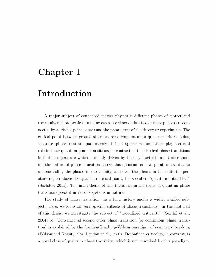
Figure 1.1: (a) The honeycomb lattice depicting monolayer graphene. The redand blue dots correspond to di↵erent sublattices. (b) The dispersion of monolayergraphene, showing only the low energy band. High energy band will be the inversionto the Ek = 0 plane. At half-filling (undoped graphene) the low energy band is com-pletely filled and high energy band is completely empty. Note the Dirac points are atK± = ±( 4⇡
3p3, 0).
points meet quadratically, and not linearly. The quadratic dispersion also leads to a
somewhat enhanced screening compared to monolayer graphene. Detailed derivation
of the dispersion of monolayer and bilayer graphene will follow.
The structure of graphene is a single layer honeycomb lattice of carbon atoms
(Fig. 1.1(a)). Each bond of this honeycomb lattice is a � bond, which is a covalent
bond between the sp2 hybridized orbitals of carbons. The remaining p orbital is
perpendicular to the plane of graphene, and this serves as the itinerant electron of
the system. This p orbital half-fills the ⇡ band, and therefore we consider one particle
per site in undoped graphene.
These facts are well represented in the following tight-binding model.
H = �tX
r2⇤A
3X
i=1
a†r br+si
+ h.c. (1.1)
Here, ⇤A and ⇤B are the sublattices of the honeycomb lattice, and si’s are the vectors
connecting nearest neighbors from ⇤A. In our coordinate system (Fig. 1.1(a)), we
4
Chapter 1: Introduction
define s1 = (0, 1), s2 = (p32,�1
2), and s3 = (�
p32,�1
2) (We set the nearest neighbor
spacing as 1). a†r (ar) and b†r (br) are the fermion creation (annihilation) operators
acting on ⇤A and ⇤B, respectively.
The energy spectrum of this Hamiltonian is shown in Fig. 1.1(b). It consist of
two distinct Dirac points, K± = ±( 4⇡3p3, 0), and the dispersion is linear at the Dirac
points. We can linearize the spectrum around the Dirac points, k = K±+p, and this
gives the expected linear dispersion of low-energy electrons.
✏p = ± |p| (1.2)
Now we turn to the dispersion of bilayer graphene. Distinguished by the stacking
structure, bilayer graphene exists in AA- and AB-stacked form. In this thesis, we
concentrate on the more common AB-stacked (or Bernal-stacked) form, where only
half of the carbon atoms are on top of each other. The tight-binding Hamiltonian for
the AB-stacked bilayer graphene is,
H = �tX
r2⇤A
3X
i=1
a†r br+si
� tX
r2⇤C
3X
i=1
c†r dr+si
� t?X
r2⇤A
a†rdr + h.c.. (1.3)
⇤C and ⇤D are the two sublattices in the additional layer, and c†(c), d†(d) are the
fermion creation (annihilation) operators acting on the sublattices. t? is the tight
binding hopping parameter between the layers which we assume is real. Note that
⇤A and ⇤D are the same in the plane of graphene.
After the same procedure as in the monolayer graphene, we obtain the low-energy
dispersion near the K± points. The new dispersion has four bands and now is
quadratic instead of being linear in the monolayer case.
✏p =1
2(±t? ±
q4|p|2 + t2?)
=
8<
:± |p|2
t2?+ O(p3)
±⇣t? + |p|2
t2?
⌘+ O(p3)
(1.4)
Note that in the first line of the above equation, two ±’s can have all four combi-
nations. There are two quadratic touching bands and two high-energy bands with a
gap of order ⇠ t?.
5
Chapter 1: Introduction
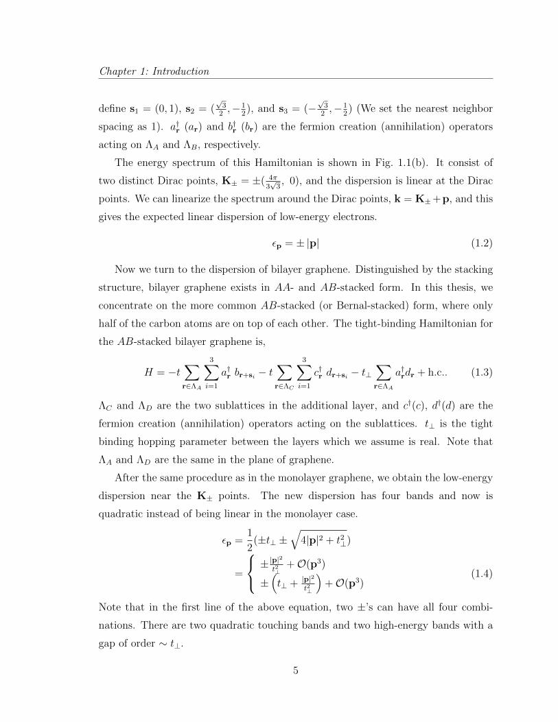
Figure 1.2: (Weitz et al., 2010) Conductivity data for suspended AB stacked bi-layer graphene. Magnetic and electric fields are both perpendicular to the plane ofgraphene. The dashed line is added to the original figure and indicates our domainof interest.
One interesting result of the dispersions calculated above is the anomalous integer
quantum Hall e↵ect seen in monolayer and bilayer graphene. Graphene systems in the
quantum Hall regime and the symmetry breaking of the SU(4) spin-valley symmetry
has been extensively investigated (Zhang et al., 2005; Novoselov et al., 2006; Nomura
and MacDonald, 2006; Bolotin et al., 2009; Weitz et al., 2010; Feldman et al., 2012).
The experimental result which will be the key motivation for Chapters 2 and 3 is also
from graphene in quantum Hall regime. Fig. 1.2 is the conductivity measurement
data in suspended bilayer graphene with both perpendicular magnetic and electric
fields (Weitz et al., 2010). One can see along the constant B-field line (depicted in
red dashed line), there exists an insulator-to-insulator phase transition. This phase
transition will be of the main focus of Chapters 2 and 3.
Finally, it is worth mentioning that graphene physics started a new field of two-
6

Chapter 1: Introduction
dimensional materials. Boron nitride, a cousin of graphene with the same honeycomb
lattice but with boron and nitrogen in the two sublattices, has been extensively stud-
ied after the advent of graphene, as well as transition-metal dichalcogenide monolay-
ers, which are single layer semiconductors. Moreover, the field is evolving into the
research of so-called “Van der Waals heterostructures,” which provides a very rich
arena of stacked two-dimensional materials (Geim and Grigorieva, 2013).
1.2 Deconfined criticality
Deconfined criticality is a critical theory of second order phase transition which is
out of the Landau-Ginzburg-Wilson paradigm (Senthil et al., 2004a,b). One classic
example of this phenomenon is the Neel to valence bond solid (VBS) transition in
square lattice. Neel phase breaks the SU(2) spin symmetry and VBS phase breaks
the translation symmetry. The symmetry of the two phases, together with their order
parameters, have very distinct structures. Therefore, the Landau’s theory of symme-
try breaking will suggest one of the following scenarios: (i) the phase transition is first
order; (ii) there are two second order phase transition, with coexistence region in the
middle; (iii) a single second order phase transition takes place with fine-tuned param-
eters. However, deconfined criticality suggests a direct continuous phase transition
without any fine-tuning of parameters. At the deconfined critical point, the theory
has fractionalized excitations, as well as a gapless ‘photon’ excitation. There is no
direct experimental signature of deconfined criticality yet, but numerical evidences
have been reported (Sandvik, 2007; Block et al., 2013).
The field theory of the Neel to VBS deconfined criticality is described in a CP 1
model. We write the Neel order parameter ~N in the CP 1 parameterization,
~N = z⇤↵~�↵�z�. (1.5)
Here, the z fields are the fractionalized spinon field, and ~� is the spin Pauli matrices.
The CP 1 parameterization has a gauge redundancy for the local phase rotation, and
therefore the spinons are coupled to a compact U(1) gauge field, aµ. The critical
7
Chapter 1: Introduction
theory of this spinon field coupled to the gauge field is written as a CP 1 model:
Lz =2X
↵
|(@µ � iaµ)z↵|2 + s|z|2 + u(|z|2)2 + (✏µ⌫�@⌫a�)2. (1.6)
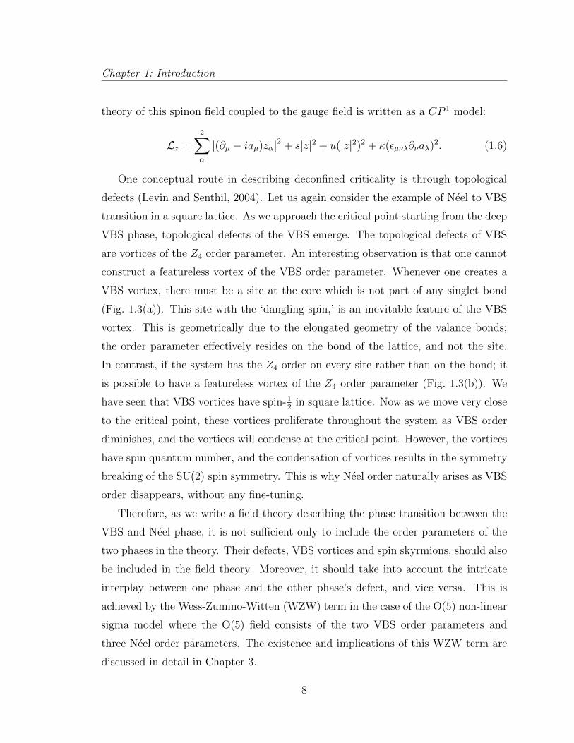
One conceptual route in describing deconfined criticality is through topological
defects (Levin and Senthil, 2004). Let us again consider the example of Neel to VBS
transition in a square lattice. As we approach the critical point starting from the deep
VBS phase, topological defects of the VBS emerge. The topological defects of VBS
are vortices of the Z4 order parameter. An interesting observation is that one cannot
construct a featureless vortex of the VBS order parameter. Whenever one creates a
VBS vortex, there must be a site at the core which is not part of any singlet bond
(Fig. 1.3(a)). This site with the ‘dangling spin,’ is an inevitable feature of the VBS
vortex. This is geometrically due to the elongated geometry of the valance bonds;
the order parameter e↵ectively resides on the bond of the lattice, and not the site.
In contrast, if the system has the Z4 order on every site rather than on the bond; it
is possible to have a featureless vortex of the Z4 order parameter (Fig. 1.3(b)). We
have seen that VBS vortices have spin-12in square lattice. Now as we move very close
to the critical point, these vortices proliferate throughout the system as VBS order
diminishes, and the vortices will condense at the critical point. However, the vortices
have spin quantum number, and the condensation of vortices results in the symmetry
breaking of the SU(2) spin symmetry. This is why Neel order naturally arises as VBS
order disappears, without any fine-tuning.
Therefore, as we write a field theory describing the phase transition between the
VBS and Neel phase, it is not su�cient only to include the order parameters of the
two phases in the theory. Their defects, VBS vortices and spin skyrmions, should also
be included in the field theory. Moreover, it should take into account the intricate
interplay between one phase and the other phase’s defect, and vice versa. This is
achieved by the Wess-Zumino-Witten (WZW) term in the case of the O(5) non-linear
sigma model where the O(5) field consists of the two VBS order parameters and
three Neel order parameters. The existence and implications of this WZW term are
discussed in detail in Chapter 3.
8
Chapter 1: Introduction
Figure 1.3: (a) VBS vortex in a square lattice, figure from Levin and Senthil (2004).The red arrows are the Z4 order parameter and the blue dashed lines are the domainboundaries. Note that there is a free-site at the core of the vortex. (b) Vortex of theZ4 order parameter at each site. In this case, the vortex is featureless.
1.3 Numerical methods in strongly correlated sys-
tems
There are many numerical methods which are widely used in strongly correlated
systems. While we study a number of model systems hoping it contains the important
physics of the much more complex real world, it is often true that we are not even able
to solve the models analytically. For example, even for the Hubbard model, which was
studied extensively for more than 50 years, analytical solutions exist only for the limit
of t/U ⌧ 1 or t/U � 1 (t is the hopping parameter and U is the on-site interaction).
Of course, many analytical methods are developed to investigate the intermediate
region t/U ⇠ 1, but these have a rather limited scope. Numerical methods may
provide “computational experiments” to certain models where analytical approach
is out of reach. Although the method itself usually cannot explain the fundamental
reasoning behind the result, it provides useful guidance and insights on constructing
microscopic theories.
A number of numerical methods stem from the Wilsonian renormalization group
(RG), each of which implements its own e�cient approximation schemes. We will
9
Chapter 1: Introduction
encounter the density matrix renormalization group (DMRG) in Chapter 4, and the
functional renormalization group (fRG) in Chapter 5.
1.3.1 Density matrix renormalization group
DMRG is a numerical method which is invented to e↵ectively calculate the ground
state of a strongly correlated system in one-dimension. In the core of its algorithm, we
use the empirical knowledge that entanglements in many-body Hamiltonian ground
states are relatively small (White, 1992; Schollwock, 2005, 2011). The renormalization
group in the name DMRG is in the sense of real space RG. However, an alternative
perspective of DMRG as a matrix product state (MPS) calculation is very useful and
can be generalized to other MPS methods such as projected entangled pair states
(PEPS) or multi-scale entanglement renormalization ansatz (MERA).
DMRG is an intrinsically one-dimensional method which is extremely powerful.
Its first result of S = 1 antiferromagnetic Heisenberg chain in White and Huse (1993)
was surprisingly accurate, considering the computing power 20 years ago. However,
the limitation of DMRG also comes from its one-dimensional nature. For its appli-
cations to two-dimensions, one needs to define a one-dimensional path covering the
system, and the calculation is not as e↵ective as in one-dimension. Two-dimensional
calculations are mostly done in cylinder geometry. The amount of computation scales
linearly as we increase the system size in the cylinder direction, but scales exponen-
tially in increasing circumference direction. Therefore, the circumference dimension
is the limiting factor in studying two-dimensional systems, and finite-size scaling is
needed for quantities for thermodynamic limit. Except for systems with very low
entanglement, computing the DMRG in the torus geometry is computationally very
costly. One can instead implement the infinite system DMRG, which performs DMRG
in an e↵ectively infinite cylinder.
DMRG also has much advantage when studying entanglement entropies of a sys-
tem (Laflorencie et al., 2006; Eisert et al., 2010; Jiang et al., 2012; Rodney et al., 2013).
Thanks to the MPS form of the DMRG wavefunction, the calculation of entanglement
entropy (and more generally the n-th Renyi entropy) is relatively straightforward.
10
Chapter 1: Introduction
We will use DMRG extensively in Chapter 4 to obtain the density profile of the
ground state and study the entanglement entropy of the system.
1.3.2 Functional renormalization group
fRG is a collection of methods which systematically approximates the Wilsonian
RG process (Salmhofer et al., 2004; Kopietz et al., 2010; Metzner et al., 2012). In the
center of fRG is the “exact flow equation”, also known as the “Wetterich equation,”
which is as follows,
d
d⇤�⇤R[�, �] =
1
2Str
⇢R⇤
h�(2)⇤R [�, �] +R⇤
i�1�. (1.7)
Here, � are the fields of the theory; it can be fermions, bosons, or a composite of
both. � is the cuto↵ dependent e↵ective action and it interpolates smoothly between
the bare action and the fully e↵ective action – when the cuto↵ scale (⇤) is at UV,
� is the bare action, and when ⇤ is at IR (⇠ 0), � becomes the e↵ective action.
The (2) in the superscript means it is a second derivative in the fields, and Str is
a supertrace which is same as the normal trace but includes a (�1) factor in the
fermionic sector. R is a cuto↵ which regulates the IR divergence. Among a number
of di↵erent cuto↵ schemes, we will be using an additive Litim cuto↵. Litim cuto↵ has
several advantages including the fact that it distorts the bare green’s function less,
and it is continuous, which is a benefit computation-wise. A detailed expression for
the Litim cuto↵ will be in the main text. This exact flow equation is exact in the
sense that this equation can be obtained by writing down the functional integration
form of the cuto↵ dependent e↵ective action, and di↵erentiating it with the cuto↵
scale.
The exact flow equation has a neat compact form, but it cannot be solved without
approximation. We have a number of approximation schemes to proceed. The first
is the vertex expansion. This procedure expands the e↵ective action in powers of the
field. As a result, we will get one flow equation for all field combinations and they
will compose an infinite hierarchy. Since it is impossible to solve the infinite sets of
equations, we truncate this hierarchy at some point. Although we have eliminated
11
Chapter 1: Introduction
infinite numbers of flow equations, the remaining equations are still very complicated.
This is because self-energy and vertex functions have momentum and frequency de-
pendence. The second approximation, derivative expansion, can be used to simplify
the each flow equations. Derivative expansion is expanding the self-energy and vertex
functions in powers of momenta and frequency, and keeping the most relevant terms
which are the lowest powers in the expansion. This gives a minimal and e�cient
scheme for obtaining critical exponents. Another popular alternative is to use a mo-
menta or frequency grid, and solving order of thousands of coupled flow equations
(Halboth and Metzner, 2000; Zanchi and Schulz, 2000; Honerkamp and Salmhofer,
2001).
One great advantage of fRG is that it is capable of considering every possible
instability in equal footing. Moreover, since the approximation scheme is very sys-
tematic, one can control the approximation relatively easily. The method of fRG will
be the central method of computation in Chapter 5.
1.4 Organization of the thesis
Starting from the next chapter, we will present a detailed study on novel quantum
phase transitions in graphene and cuprates, building upon the materials from this
chapter. The remainder of the thesis is organized as follows.
In Chapter 2 we propose that bilayer graphene can provide an experimental re-
alization of deconfined criticality. Current experiments indicate the presence of Neel
order in the presence of a moderate magnetic field. The Neel order can be destabilized
by application of a transverse electric field. The resulting electric field induced state
is likely to have valence bond solid order, and the transition can acquire the emergent
fractionalized and gauge excitations of deconfined criticality.
In Chapter 3 we consider the interplay between the antiferromagnetic and Kekule
valence bond solid orderings in the zero energy Landau levels of neutral monolayer
and bilayer graphene. We establish the presence of Wess-Zumino-Witten terms be-
tween these orders: this implies that their quantum fluctuations are described by
12

Chapter 1: Introduction
the deconfined critical theories of quantum spin systems. We present implications
for experiments, including the possible presence of excitonic superfluidity in bilayer
graphene.
In Chapter 4 we study a recently proposed quantum dimer model for the pseudo-
gap metal state of the cuprates. The model contains bosonic dimers, representing a
spin-singlet valence bond between a pair of electrons, and fermionic dimers, represent-
ing a quasiparticle with spin-1/2 and charge +e. By density matrix renormalization
group calculations on a long but finite cylinder, we obtain the ground state density
distribution of the fermionic dimers for a number of di↵erent total densities. From
the Friedel oscillations at open boundaries, we deduce that the Fermi surface consists
of small hole pockets near (⇡/2, ⇡/2), and this feature persists up to doping density
1/16. We also compute the entanglement entropy and find that it closely matches
the sum of the entanglement entropies of a critical boson and a low density of free
fermions. Our results support the existence of a fractionalized Fermi liquid (FL*) in
this model.
In Chapter 5 we present a functional renormalization group analysis of a quantum
critical point in two-dimensional metals involving Fermi surface reconstruction due
to the onset of spin-density wave order. Its critical theory is controlled by a fixed
point in which the order parameter and fermionic quasiparticles are strongly coupled
and acquire spectral functions with a common dynamic critical exponent. We obtain
results for critical exponents and for the variation in the quasiparticle spectral weight
around the Fermi surface. Our analysis is implemented on a two-band variant of
the spin-fermion model which will allow comparison with sign-problem-free quantum
Monte Carlo simulations.
13
Chapter 2
Deconfined criticality in bilayer
graphene
2.1 Introduction
Undoped graphene, in both its monolayer and bilayer forms, is nominally a semi-
metal. However, upon application of a moderate magnetic field, it turns into an
insulator (Checkelsky et al., 2009) (in the quantum Hall terminology, this state has
filling fraction ⌫ = 0). Evidence has been accumulating from recent experiments
(Weitz et al., 2010; Freitag et al., 2012; Velasco et al., 2012; Young et al., 2012;
Maher et al., 2013; Freitag et al., 2013; Young et al., 2014) that the insulator has
symmetry breaking due to the appearance of antiferromagnetic long-range order.
Because of the applied magnetic field, the antiferromagnetic order is expected to lie
in the plane orthogonal to the magnetic field, along with a ferromagnetic “canting”
of the spins along the direction of the magnetic field: this state is therefore referred
to as a canted antiferromagnet (CAF). For the case of bilayer graphene, experiments
(Weitz et al., 2010; Freitag et al., 2012; Velasco et al., 2012; Maher et al., 2013; Freitag
et al., 2013) have also induced what appears to be a quantum phase transition out
of the CAF state. This is done by applying an electric field transverse to the layers,
leading to states with layer polarization of electric charge, but presumably without
14
Chapter 2: Deconfined criticality in bilayer graphene
(a) (b) (c)
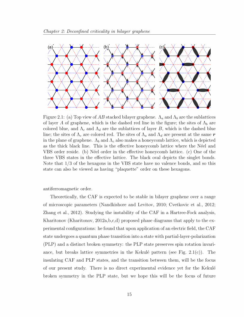
Figure 2.1: (a) Top view of AB stacked bilayer graphene. ⇤a and ⇤b are the sublatticesof layer A of graphene, which is the dashed red line in the figure; the sites of ⇤b arecolored blue, and ⇤c and ⇤d are the sublattices of layer B, which is the dashed blueline; the sites of ⇤c are colored red. The sites of ⇤a and ⇤d are present at the same rin the plane of graphene. ⇤b and ⇤c also makes a honeycomb lattice, which is depictedas the thick black line. This is the e↵ective honeycomb lattice where the Neel andVBS order reside. (b) Neel order in the e↵ective honeycomb lattice. (c) One of thethree VBS states in the e↵ective lattice. The black oval depicts the singlet bonds.Note that 1/3 of the hexagons in the VBS state have no valence bonds, and so thisstate can also be viewed as having “plaquette” order on these hexagons.
antiferromagnetic order.
Theoretically, the CAF is expected to be stable in bilayer graphene over a range
of microscopic parameters (Nandkishore and Levitov, 2010; Cvetkovic et al., 2012;
Zhang et al., 2012). Studying the instability of the CAF in a Hartree-Fock analysis,
Kharitonov (Kharitonov, 2012a,b,c,d) proposed phase diagrams that apply to the ex-
perimental configurations: he found that upon application of an electric field, the CAF
state undergoes a quantum phase transition into a state with partial-layer-polarization
(PLP) and a distinct broken symmetry: the PLP state preserves spin rotation invari-
ance, but breaks lattice symmetries in the Kekule pattern (see Fig. 2.1(c)). The
insulating CAF and PLP states, and the transition between them, will be the focus
of our present study. There is no direct experimental evidence yet for the Kekule
broken symmetry in the PLP state, but we hope this will be the focus of future
15
Chapter 2: Deconfined criticality in bilayer graphene
experiments.
From the perspective of symmetry, we are therefore investigating the quantum
phase transition between two insulating states in an electronic model that has spin
rotation symmetry and the space group symmetries of the honeycomb lattice. One
insulator breaks spin rotation symmetry by the appearance of antiferromagnetic long-
range order in the two-sublattice pattern shown in Fig. 2.1(b): we will henceforth
refer to this insulator as the Neel state. The second insulator breaks the space group
symmetry alone in the Kekule pattern of Fig. 2.1(c). A direct quantum phase tran-
sition between two insulators with precisely the same symmetries was first discussed
some time ago in Read and Sachdev (1990) in the very di↵erent context of correlated
electron models inspired by the cuprate high-temperature superconductors. In these
models, the Kekule state is referred to as a valence bond solid (VBS), as the space
group symmetry is broken by singlet valence bonds between spins on the sites of the
honeycomb lattice; we include the “plaquette” resonating state within the class of
VBS states, and it breaks the honeycomb lattice symmetry in the same pattern.
More recently, the Neel-VBS transition has been identified (Senthil et al., 2004a,b)
as a likely candidate for “deconfined criticality.” In this theory, the low-energy exci-
tations in the vicinity of the transition are described by neutral excitations carrying
spin S = 1/2 (“spinons”) coupled to each other by the “photon” of an emergent U(1)
gauge field. The quantum transition itself is either second order or weakly first order;
in either case, there is evidence for the presence of the emergent gauge excitations
(Sandvik, 2007; Block et al., 2013).
In the present chapter, we will apply a strong coupling perspective to models on
the bilayer honeycomb lattice linked to the physics of bilayer graphene. Our analysis
therefore complements that of Kharitonov, who perturbatively examined the e↵ect of
interactions after projecting to the lowest Landau level. We also note other theoretical
studies by Roy and collaborators (Roy, 2013, 2014; Roy et al., 2014), which do not
project to the lowest Landau level. Our perspective is more suited to addressing the
nature of quantum fluctuations near the quantum phase transition, and for describing
the possible emergence of exotic varieties of fractionalization. We will discuss some
16
Chapter 2: Deconfined criticality in bilayer graphene
of the experimental consequences of this new perspective in Chapter 2.8.
We will introduce our lattice model on the bilayer honeycomb lattice in Chap-
ter 2.2. We assume that the strongest coupling in the model is the on-site Hubbard
repulsion U , and perform a traditional 1/U expansion to obtain an e↵ective spin model
on the same lattice. In Chapter 2.3, we examine this spin model in a spin-wave ex-
pansion, and determine regimes where the Neel order is suppressed. An alternative
e↵ective spin model, related to those examined in recent numerical work, is studied
in Chapter 2.4. We study the geometric phases between the Neel and VBS orders in
Chapters 2.5 and 2.6, and comment on the structure of vortices in the VBS order in
Chapter 2.7.
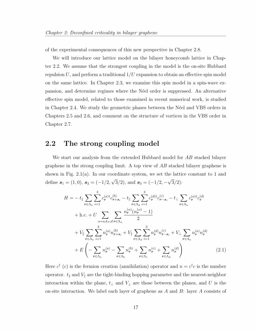
2.2 The strong coupling model
We start our analysis from the extended Hubbard model for AB stacked bilayer
graphene in the strong coupling limit. A top view of AB stacked bilayer graphene is
shown in Fig. 2.1(a). In our coordinate system, we set the lattice constant to 1 and
define s1 = (1, 0), s2 = (�1/2,p3/2), and s3 = (�1/2,�p3/2):
H =� tkX
r2⇤a
3X
i=1
c(a)†r c(b)r+si
� tkX
r2⇤d
3X
i=1
c(d)†r c(c)r�si
� t?X
r2⇤a
c(a)†r c(d)r
+ h.c. + UX
↵=a,b,c,d
X
r2⇤↵
n(↵)r (n(↵)
r � 1)
2
+ VkX
r2⇤a
3X
i=1
n(a)r n(b)
r+si
+ VkX
r2⇤d
3X
i=1
n(d)r n(c)
r�si
+ V?X
r2⇤a
n(a)r n(d)
r
+ E
�X
r2⇤a
n(a)r �
X
r2⇤b
n(b)r +
X
r2⇤c
n(c)r +
X
r2⇤d
n(d)r
!(2.1)
Here c† (c) is the fermion creation (annihilation) operator and n = c†c is the number
operator. tk and Vk are the tight-binding hopping parameter and the nearest-neighbor
interaction within the plane, t? and V? are those between the planes, and U is the
on-site interaction. We label each layer of graphene as A and B: layer A consists of
17
Chapter 2: Deconfined criticality in bilayer graphene
sublattices ⇤a and ⇤b, and layer B consists of sublattices ⇤c and ⇤d. Only one of
the sublattices in each layer has common in-plane coordinate in AB stacked bilayer
graphene, and we set those to be ⇤a and ⇤d. Elsewhere in the literature, the site
labels a, b, c, and d are often referred to as A1, B1, A2, and B2, respectively,
meaning sublattice A(B) or layer 1(2). However, we find it more convenient to use
the compact notation a, b, c, d. Hopping and interaction between the layers only
occurs between these sublattices. We also include an electric field transverse to the
plane of graphene, pointing from layer A to layer B. The electric field is minimally
coupled to the density of the fermions with coupling E. We assume that E is also
smaller than U , and so both layers will be half-filled at leading order in 1/U , and the
e↵ective Hamiltonian can be expressed only in terms of spin operators on the sites.
The subleading 1/U corrections will induce terms in the e↵ective Hamiltonian, but
also induce a polarization in the layer density when computed in terms of the bare
electron operators.
Our Hamiltonian does not explicitly include the influence of an applied magnetic
field. Such a field will modify H in two ways, via a Peierls phase factor on the
hopping terms tk,?, and a Zeeman coupling. In the context of our strong coupling
expansion, the influence of the Peierls phases will only be to modify the coe�cients of
ring-exchange terms in the e↵ective spin Hamiltonian. However, such ring-exchange
terms only appear at sixth order in tk, and this is higher order than our present
analysis; so we can safely drop the Peierls phases. The Zeeman term commutes with
all other terms in H, and so does not modify the analysis below, and can be included
as needed in the final e↵ective Hamiltonian.
From this Hamiltonian, we work on the strong coupling limit, where tk, t? ⌧U, V , and perform the t/U expansion up to O(t4/U3) order. In this expansion we
assume both tk and t? are much smaller than U , although this is not well satisfied
in the experiment (also, there is a significant di↵erence in the values of the hopping
parameters from Zhang et al. (2008), tk ⇠ 3.0 eV, t? ⇠ 0.40 eV). There are numerous
works on the t/U expansion of the Hubbard model in various lattices, including the
classic work of MacDonald et al. (1988) and Takahashi (1977) in square lattice. Extra
18
Chapter 2: Deconfined criticality in bilayer graphene
care is needed while dealing the similar procedure with the above model since we have
included nearest neighbor interaction and the lattice structure is more complicated.
First, we organize the Hamiltonian in Eq. (2.1) as H = HU +Ht, where HU is the
interaction term and Ht is the kinetic term. We consider Ht as the perturbation and
rearrange it by the change of interaction energy through the hopping process,
Ht =X
�
[T� + T��] . (2.2)
T� is the sum of all hopping terms that increases the interaction energy by �U . For
notational convenience, we restrict � to be positive and collect the decreasing energy
processes to T�� with an explicit negative sign.
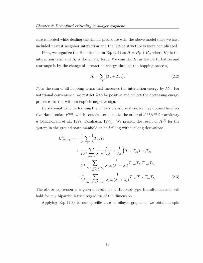
By systematically performing the unitary transformation, we may obtain the e↵ec-
tive Hamiltonian H(n), which contains terms up to the order of tn+1/Un for arbitrary
n (MacDonald et al., 1988; Takahashi, 1977). We present the result of H(3) for the
system in the ground-state manifold at half-filling without long derivation:
H(3)GS,HF =� 1
U
X
�
1
�T��T�
+1
2U3
X
�1,�2
1
�1�2
✓1
�1+
1
�2
◆T��1T�1T��2T�2
� 1
U3
X
�1+�2=�3+�4�1 6=�3
1
�1�4(�1 � �3)T��1T�3T��2T�4
� 1
U3
X
�1+�2=�3+�4
1
�1�4(�1 + �2)T��1T��2T�3T�4 . (2.3)
The above expression is a general result for a Hubbard-type Hamiltonian and will
hold for any bipartite lattice regardless of the dimension.
Applying Eq. (2.3) to our specific case of bilayer graphene, we obtain a spin
19

Chapter 2: Deconfined criticality in bilayer graphene
Hamiltonian that contains every term up to the order of t4/U3,
H = JkX
r2⇤a
3X
i=1
~S(a)r · ~S(b)
r+si
+ JkX
r2⇤d
3X
i=1
~S(d)r · ~S(c)
r�si
+ J?X
r2⇤a
~S(a)r · ~S(d)
r + J2X
↵=a,b,c,d
X
r2⇤↵
3X
i=1
~S(↵)r · ~S(↵)
r+ti
+ J⇥X
r2⇤a
3X
i=1
~S(a)r · ~S(c)
r�si
+ J⇥X
r2⇤d
3X
i=1
~S(d)r · ~S(b)
r+si
, (2.4)
with the exchange couplings as,
Jk =4 t2k
U � Vk �⇣
V 2?
U�Vk
⌘ , J? =4 t2?
U � V? �⇣
E2
U�V?
⌘ ,
J2 =4 t4k
(U � Vk)2 � V 2?
2(U � Vk)
�(U � Vk)2 + V 2
?�
�(U � Vk)2 � V 2
?�2 � 1
U
!,
(2.5)
and,
J⇥ =4 t2k t
2?
⇣(U � V 2
k )2 � V 2
?⌘2 �
(U � V?)2 � E2
�2((U + V?)2 � E2)
⇥
�(U � V?)2(U + V?)
⇥(U2 + V?U � VkV?)(U � Vk)2 � V 2
?(U2 � (4Vk � V?)U
+(2Vk � V?)Vk)⇤� E2
⇥2U5 � (4Vk + 5V?)U4 + (2V 2
k + 13VkV? + 8V 2?)U
3
� V?(Vk + V?)(11Vk + 2V?)U2 + V?(Vk + V?)(3Vk � V?)(Vk + 2V?)U
�V 2?(V
3k + 3V 2
k V? � VkV 2? + V 3
?)⇤+ E4(U � V?)[(U � Vk)2 + V 2
?] . (2.6)
We have additionally defined t1 = s2 � s3, t2 = s3 � s1, and t3 = s1 � s2. Without
the electric field, the lattice symmetry guarantees the J⇥ coupling in ~S(a)r · ~S(c)
r�si
and ~S(d)r · ~S(b)
r+si
to be the same. However, when the field is turned on, the layer
symmetry breaks and the two J⇥ values become di↵erent. Here, we take the average
value for simplicity. This will not change the qualitative behavior unless E is very
large. Di↵erent exchange couplings defined in Eq. (2.4) are shown schematically
in Fig. 2.2. We work in the parameter range where all four exchange couplings
20
Chapter 2: Deconfined criticality in bilayer graphene
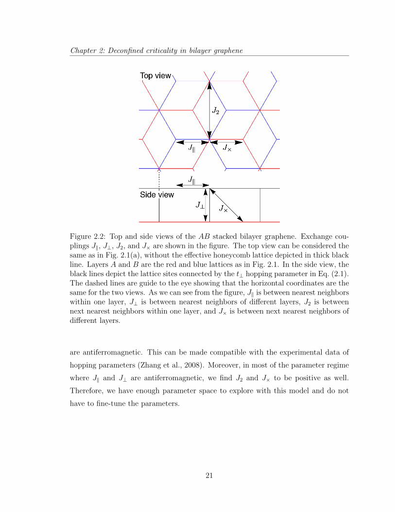
Figure 2.2: Top and side views of the AB stacked bilayer graphene. Exchange cou-plings Jk, J?, J2, and J⇥ are shown in the figure. The top view can be considered thesame as in Fig. 2.1(a), without the e↵ective honeycomb lattice depicted in thick blackline. Layers A and B are the red and blue lattices as in Fig. 2.1. In the side view, theblack lines depict the lattice sites connected by the t? hopping parameter in Eq. (2.1).The dashed lines are guide to the eye showing that the horizontal coordinates are thesame for the two views. As we can see from the figure, Jk is between nearest neighborswithin one layer, J? is between nearest neighbors of di↵erent layers, J2 is betweennext nearest neighbors within one layer, and J⇥ is between next nearest neighbors ofdi↵erent layers.
are antiferromagnetic. This can be made compatible with the experimental data of
hopping parameters (Zhang et al., 2008). Moreover, in most of the parameter regime
where Jk and J? are antiferromagnetic, we find J2 and J⇥ to be positive as well.
Therefore, we have enough parameter space to explore with this model and do not
have to fine-tune the parameters.
21
Chapter 2: Deconfined criticality in bilayer graphene
2.3 Spin-wave expansion
Previous studies of the bilayer antiferromagnet have focused on the square lattice
(Hida, 1990; Sandvik et al., 1995; Chubukov and Morr, 1995; Millis and Monien, 1996;
Wang et al., 2006) where the sites are stacked directly on top of each other. In these
models, as the interlayer coupling is increased, there is eventually a transition from
the Neel state to a “trivial” paramagnet in which the ground state is approximately
the product of interlayer valence bonds between superposed spins. However, here we
are considering a staggered stacking, in which no such trivial one-to-one identifica-
tion of spins between the two layers is possible. Any pairing of spins must break a
lattice symmetry, and this is a simple argument for the appearance of a VBS state.
Nevertheless, it is useful to apply the spin-wave expansion used for the square lattice
(Hida, 1990; Chubukov and Morr, 1995), and study how the intra- and inter-layer
couplings modify the staggered magnetization. This will help us determine the pa-
rameter regime over which the Neel order decreases, and a possible VBS state can
appear. However, a description of the transition to, and structure of, the VBS state
is beyond the regime of applicability of the spin-wave expansion.
Among the four exchange couplings listed in Eqs. (2.5) and (2.6), only J? and J⇥
depend on the electric field strength, E. The electric field breaks the layer symmetry,
so it is reasonable that E is only included in the exchange coupling between di↵erent
layers. We start from the Neel phase and calculate the staggered magnetization of
the bilayer graphene as a function of either J?, J⇥, or E. Since our starting point is
an SU(2) symmetry broken state, we use the Holstein-Primako↵ representation.
Starting from the e↵ective spin Hamiltonian derived in Eq. (2.4), we perform
the 1/S expansion (where S is the magnitude of the spin, and we are interested
in S = 1/2) about the antiferromagnetically ordered state by expressing the spin
22
Chapter 2: Deconfined criticality in bilayer graphene
operators in terms of bosons, a, b, c, d:
S(a)z = S � a†a, S(a)
+ =p2S(1� a†a/(2S))1/2a,
S(b)z = �S + b†b, S(b)
+ =p2Sb†(1� b†b/(2S))1/2,
S(c)z = S � c†c, S(c)
+ =p2S(1� c†c/(2S))1/2c,
S(d)z = �S + d†d, S(d)
+ =p2Sd†(1� d†d/(2S))1/2. (2.7)
Then, to the needed order, the Hamiltonian is,
H = JkX
r2⇤a
3X
i=1
⇣�S2 + S(a†rar + b†r+s
i
br+si
+ a†rb†r+s
i
+ arbr+si
)⌘
+ JkX
r2⇤d
3X
i=1
⇣�S2 + S(d†rdr + c†r�s
i
cr�si
+ d†rc†r�s
i
+ drcr�si
)⌘
+ J?X
r2⇤a
��S2 + S(a†rar + d†rdr + a†rd†r + ardr
�
+ J2X
r2⇤a
3X
i=1
⇣S2 + S(�a†rar � a†r+t
i
ar+ti
+ a†rar+ti
+ a†r+ti
ar)⌘
+ J2X
r2⇤b
3X
i=1
⇣S2 + S(�b†rbr � b†r+t
i
br+ti
+ b†rbr+ti
+ b†r+ti
br)⌘
+ J2X
r2⇤c
3X
i=1
⇣S2 + S(�c†rcr � c†r+t
i
cr+ti
+ c†rcr+ti
+ c†r+ti
cr)⌘
+ J2X
r2⇤d
3X
i=1
⇣S2 + S(�d†rdr � d†r+t
i
dr+ti
+ d†rdr+ti
+ d†r+ti
dr)⌘
+ J⇥X
r2⇤a
3X
i=1
⇣S2 + S(�a†rar � c†r�s
i
cr�si
+ a†rcr�si
+ c†r�si
ar)⌘
+ J⇥X
r2⇤d
3X
i=1
⇣S2 + S(�d†rdr � b†r+s
i
br+si
+ d†rbr+si
+ b†r+si
dr)⌘.
(2.8)
We write this in momentum space as,
H = �3NS(S + 1)(2Jk + J?/3� 4J2 � 2J⇥) + SX
k
†kM(k) k, (2.9)
23
Chapter 2: Deconfined criticality in bilayer graphene
where N is the number of sites in ⇤a, k is the boson spinor k = (ak, ck, b†�k, d
†�k),
and
M(k) =
0
BBBBB@
J(k) + J? J⇥�(�k) Jk�(k) J?
J⇥�(k) J(k) 0 Jk�(k)
Jk�(�k) 0 J(k) J⇥�(�k)J? Jk�(�k) J⇥�(k) J(k) + J?
1
CCCCCA,
with
J(k) = Jk + J2�(k)� 3J⇥,
�(k) =3X
i=1
eik·si ,
�(k) = �6 + 23X
i=1
cos (k · ti) .
The Hamiltonian can be diagonalized by a bosonic version of the Bogoliubov trans-
formation (which is not a unitary transformation) as described in Sachdev (1992).
Now the staggered magnetization of the bilayer graphene can be obtained from the
diagonalized Hamiltonian. The expression for the magnetization is very complicated
with all four exchange couplings, and hard to write down in a closed form. Therefore
we present numerical values for a selected set of parameters. Fig. 2.3 shows the
calculated magnetization as a function of J? and J⇥ for parameters Jk/U = 0.089,
J2/U = 0.0095, J⇥/U = 0.0018, and J?/U = 0.028 (unless one is the variable for the
graph). These correspond to tk/U = 0.1, t?/U = 0.07, Vk/U = 0.4, and V?/U = 0.3
for the parameters in the extended Hubbard model. Since the sublattices ⇤a(⇤d) and
⇤b(⇤c) are not symmetric in AB-stacked bilayer graphene, they will in general have
di↵erent magnetization, and therefore are plotted separately (for example, sites in
⇤a(⇤d) has coordination number of 4, whereas the sites in ⇤b(⇤c) has 3). As depicted
in Fig. 2.1, the Neel and VBS states of interest reside in ⇤b and ⇤c. We are therefore
more interested in the magnetization of ⇤b than ⇤a.
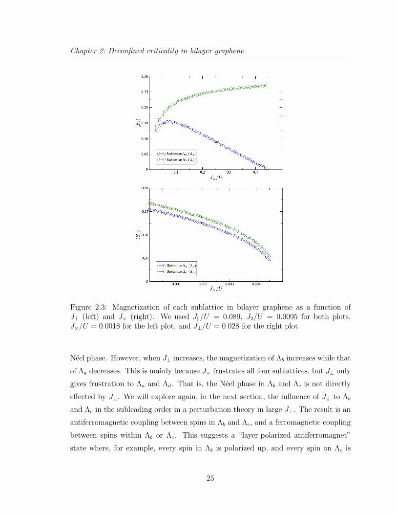
We observe that the magnetization in each sublattice decreases as J⇥ increases.
This is reasonable in the sense that antiferromagnetic J⇥ increases frustration of the
24
Chapter 2: Deconfined criticality in bilayer graphene
Figure 2.3: Magnetization of each sublattice in bilayer graphene as a function ofJ? (left) and J⇥ (right). We used Jk/U = 0.089, J2/U = 0.0095 for both plots,J⇥/U = 0.0018 for the left plot, and J?/U = 0.028 for the right plot.
Neel phase. However, when J? increases, the magnetization of ⇤b increases while that
of ⇤a decreases. This is mainly because J⇥ frustrates all four sublattices, but J? only
gives frustration to ⇤a and ⇤d. That is, the Neel phase in ⇤b and ⇤c is not directly
e↵ected by J?. We will explore again, in the next section, the influence of J? to ⇤b
and ⇤c in the subleading order in a perturbation theory in large J?. The result is an
antiferromagnetic coupling between spins in ⇤b and ⇤c, and a ferromagnetic coupling
between spins within ⇤b or ⇤c. This suggests a “layer-polarized antiferromagnet”
state where, for example, every spin in ⇤b is polarized up, and every spin on ⇤c is
25
Chapter 2: Deconfined criticality in bilayer graphene
polarized down. So the increased magnetization of ⇤b can be explained in this manner.
This is not the scenario we expect in the Neel to VBS phase transition, because the
Neel order is becoming stronger with an increase of J?. However, there will not be
a case where J? increases alone because J⇥ coupling will also increase as we increase
the electric field. This J⇥ gives frustration to the layer-polarized order, which will
result in the decrease of the staggered magnetization. Note that, in any case, the
magnetization is smaller for ⇤a than ⇤b, which contradicts our usual intuition that
a larger coordination number agrees better with the mean-field result. However, this
result is in accordance with Lang et al. (2012), where they find the same behavior
by quantum Monte Carlo simulation for a Heisenberg model with only Jk and J?
couplings, but in a wide range of J?.
To obtain the staggered magnetization for more realistic states, including the
ones in experiments, we need to consider the change of J? and J⇥ in a consistent
manner. This is done by tuning a single parameter E, the coupling of electric field.
Using the expressions in Eqs. (2.5) and (2.6), we can find the magnetizations for each
sublattice as a function of E. As for the previous results, we only show numerical
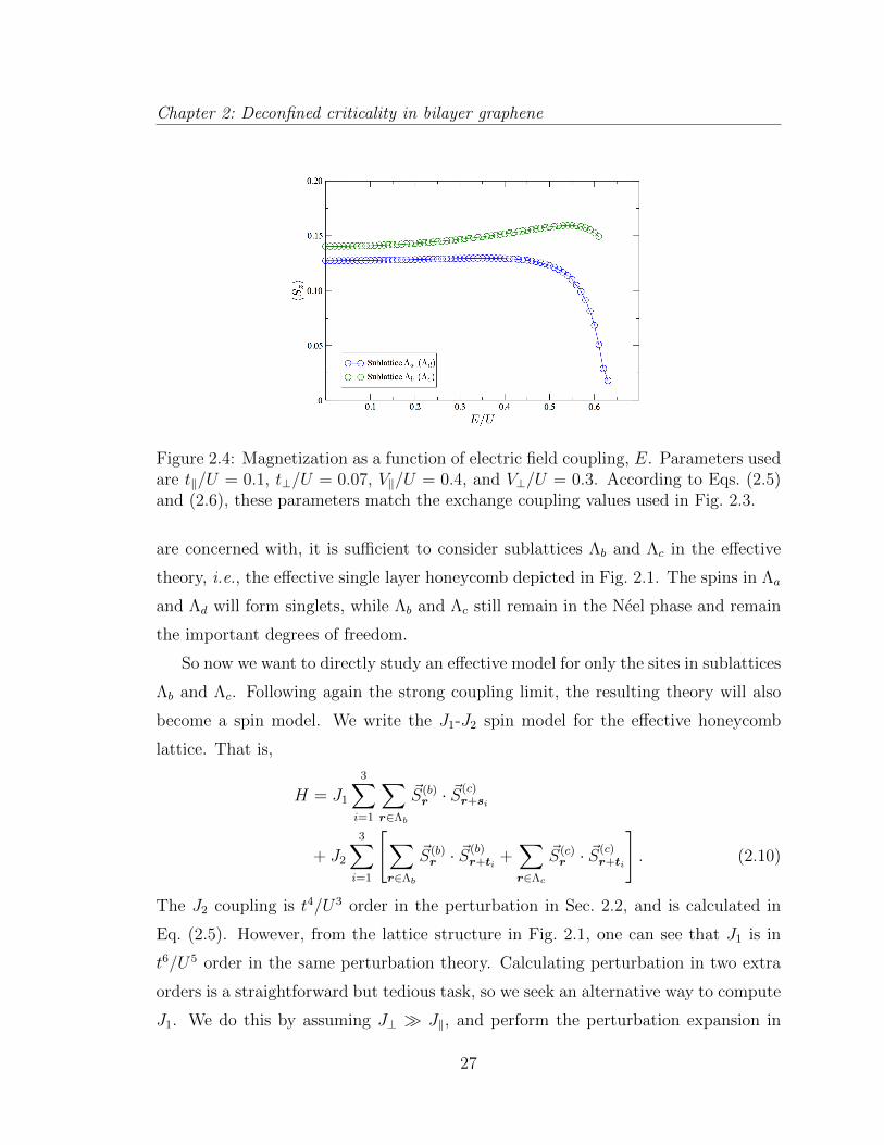
results for selected parameters. Fig. 2.4 shows the result for the same parameters as
in Fig. 2.3, tk/U = 0.1, t?/U = 0.07, Vk/U = 0.4, and V?/U = 0.3. We observe
the magnetization of ⇤a decrease drastically from E ⇠ 0.50U and that of ⇤b starts
to decrease from E ⇠ 0.55U , although we cannot see a significant decrease in ⇤b
before the Holstein-Primako↵ theory breaks down. However, from the two plots in
Fig. 2.3 where the magnetization of ⇤b saturates as increasing J? and vanishes as
increasing J⇥, we can argue that when both J?, J⇥ are increasing the magnetization
will decrease eventually, and Fig. 2.4 is showing the onset of the decrease. This result
shows explicitly how the Neel order decreases as the electric field increases.
2.4 J1-J2 model
The fact that the magnetization of ⇤a and ⇤d decreases faster than that of ⇤b and
⇤c in the previous section can be taken as evidence that, in the phase transition we
26
Chapter 2: Deconfined criticality in bilayer graphene
Figure 2.4: Magnetization as a function of electric field coupling, E. Parameters usedare tk/U = 0.1, t?/U = 0.07, Vk/U = 0.4, and V?/U = 0.3. According to Eqs. (2.5)and (2.6), these parameters match the exchange coupling values used in Fig. 2.3.
are concerned with, it is su�cient to consider sublattices ⇤b and ⇤c in the e↵ective
theory, i.e., the e↵ective single layer honeycomb depicted in Fig. 2.1. The spins in ⇤a
and ⇤d will form singlets, while ⇤b and ⇤c still remain in the Neel phase and remain
the important degrees of freedom.
So now we want to directly study an e↵ective model for only the sites in sublattices
⇤b and ⇤c. Following again the strong coupling limit, the resulting theory will also
become a spin model. We write the J1-J2 spin model for the e↵ective honeycomb
lattice. That is,
H = J1
3X
i=1
X
r2⇤b
~S(b)r · ~S(c)
r+si
+ J2
3X
i=1
"X
r2⇤b
~S(b)r · ~S(b)
r+ti
+X
r2⇤c
~S(c)r · ~S(c)
r+ti
#. (2.10)
The J2 coupling is t4/U3 order in the perturbation in Sec. 2.2, and is calculated in
Eq. (2.5). However, from the lattice structure in Fig. 2.1, one can see that J1 is in
t6/U5 order in the same perturbation theory. Calculating perturbation in two extra
orders is a straightforward but tedious task, so we seek an alternative way to compute
J1. We do this by assuming J? � Jk, and perform the perturbation expansion in
27
Chapter 2: Deconfined criticality in bilayer graphene
Jk/J?. Admittedly, because tk is actually significantly smaller than t? in graphene,
this perturbation expansion is rather far from the experimental situation; however,
the regime Jk � J? o↵ers a tractable limit for studying the phase transition using
existing results so seems worthwhile to explore. In the opposite limit of J? ⌧ Jk,
qualitatively, the magnetization of ⇤a and ⇤b will be the same although they may be
small. Therefore our assumption of J? � Jk will be true in regions where hS(b)z i �
hS(a)z i. In Fig. 2.4, this is the case when E/U > 0.55. This means that the large J?
limit is more valid near the phase transition, and thus suits our purpose of studying
the vicinity of the transition point.
The Jk/J? expansion has two contributions to the e↵ective honeycomb lattice in
the order of J2k/J?, one to the J1 term and the other to the J2 term. The contributions
from the Jk/J? expansion follows from the e↵ective Hamiltonian method (Cohen-
Tannoudji et al., 1992),
J1 =J2k
J?=
4 t4kt2?
U � V? �⇣
E2
U�V?
⌘
⇣U � Vk �
⇣V 2?
U�Vk
⌘⌘2 ,
J2 = �J2k
2J?= �2 t4k
t2?
U � V? �⇣
E2
U�V?
⌘
⇣U � Vk �
⇣V 2?
U�Vk
⌘⌘2 . (2.11)
From our assumption that Jk and J? are antiferromagnetic, it follows that the contri-
bution to J1 is antiferromagnetic and J2 is ferromagnetic. For a complete description
for the J1 � J2 model in the e↵ective honeycomb lattice up to the desired order, we
need to add the J2 contributions from the t/U expansion and Jk/J? expansion. The
28
Chapter 2: Deconfined criticality in bilayer graphene
final J1 � J2 model will be Eq. (2.10) with exchange couplings of
J1 =4 t4kt2?
U � V? �⇣
E2
U�V?
⌘
⇣U � Vk �
⇣V 2?
U�Vk
⌘⌘2 ,
J2 =4 t4k
(U � Vk)2 � V 2?
2(U � Vk)
�(U � Vk)2 + V 2
?�
�(U � Vk)2 � V 2
?�2 � 1
U
!
� 2 t4kt2?
U � V? �⇣
E2
U�V?
⌘
⇣U � Vk �
⇣V 2?
U�Vk
⌘⌘2 . (2.12)
The ground state of the above J1-J2 model can only be solved numerically. How-
ever, qualitative behaviors can be studied from the E dependence of J1 and J2. Di-
rectly from Eq. (2.12), one can see that J1 decreases and J2 increases as E increases.
Since the first term of J2 in Eq. (2.12) is positive, we always have a window of E where
both J1 and J2 are positive. Inside that window, the ratio of J2/J1 will increase as E
increases, until J1 decreases to 0. We know that for J2/J1 ⌧ 1 the ground state will
be a Neel state, including when J2 < 0, where J2 supports the Neel state. However, a
positive J2 starts to frustrate the Neel phase as J2/J1 increases. This will eventually
destroy the Neel state at a critical value of J2/J1, and a phase transition will occur.
Numerically, the J1-J2 model in a honeycomb lattice has recently been investigated
via a variety of methods (Clark et al., 2011; Albuquerque et al., 2011; Ganesh et al.,
2013; Zhu et al., 2013; Gong et al., 2013), and related models have been studied in
Pujari et al. (2013) and Lang et al. (2013). These studies all find a transition out of
the Neel state to a Kekule VBS state (or the closely related plaquette state, which
has the same pattern on symmetry breaking on the honeycomb lattice). Ganesh et al.
(2013), Zhu et al. (2013), and Gong et al. (2013) tune J2/J1, and find evidence for
an apparent second-order phase transition from Neel state at small J2/J1 to VBS
state at larger J2/J1, where the critical value J2/J1 ⇠ 0.22—0.26. The studies can
be therefore considered as the numerical analysis of our J1-J2 model in the window
of E where J1, J2 > 0. Since the critical value of J2/J1 in the DMRG study can be
always reached in our model through a certain value of E, we may argue that the
same phase transition from Neel to VBS happens in the bilayer graphene system as
29
Chapter 2: Deconfined criticality in bilayer graphene
well, when tuning the electric field. So the J1-J2 model in the e↵ective honeycomb
lattice not only supports the Neel to VBS phase transition in the bilayer graphene,
but also provides indirect evidence that the transition is in the deconfined category.
2.5 Geometric phases
Our analysis so far has examined the potential instability of the Neel phase to
a “quantum disordered” phase, which preserves spin rotation invariance. General
arguments were made in Read and Sachdev (1990) that any such phase in a model
with the symmetry of the honeycomb lattice must have VBS order: these arguments
relied on Berry phases of “hedgehog” tunneling events in the Neel order. In Fu
et al. (2011) (see also Yao and Lee (2010)), these arguments were recast in terms of
geometric phases associated with skyrmion textures, which led to a coupling in the
action between the temporal derivative of the VBS order and the skyrmion density
in the Neel order. This section will obtain a similar term for the case of the bilayer
antiferromagnet. This term will be obtained in a weak coupling model, and we will
comment on the relationship to the strong coupling results at the end of the present
section.
Since we already know the ground states around the critical point are Neel and
VBS states, we write a weak coupling Hamiltonian and later include interaction e↵ects
and the electric field as a Neel and VBS mean-field order parameter. The weak
coupling Hamiltonian in a bilayer honeycomb lattice is merely a tight-binding model.
Using the parameters and operators defined as in Sec. 2.2, this is
Hw =� tkX
r2⇤a
3X
i=1
c(a)†r c(b)r+si
� tkX
r2⇤d
3X
i=1
c(d)†r c(c)r�si
� t?X
r2⇤a
c(a)†r c(d)r � t2X
r2⇤b
3X
i=1
c(b)†r c(c)r+si
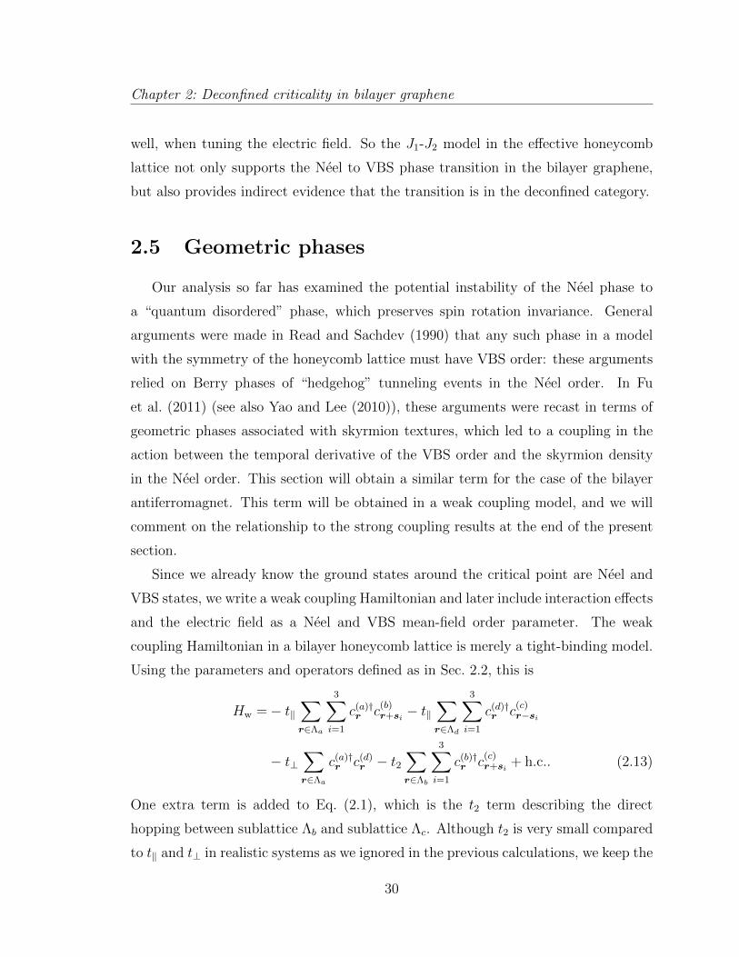
+ h.c.. (2.13)
One extra term is added to Eq. (2.1), which is the t2 term describing the direct
hopping between sublattice ⇤b and sublattice ⇤c. Although t2 is very small compared
to tk and t? in realistic systems as we ignored in the previous calculations, we keep the
30
Chapter 2: Deconfined criticality in bilayer graphene
t2 term in the current section to use it as a parameter interpolating between bilayer
and monolayer graphene (McCann and Fal’ko, 2006).
The band structure of this Hamiltonian consists of four bands where two of them
quadratically touch at the two K points, which we label them as K± = ±(0, 4⇡3p3). At
half-filling, the Fermi level is right at the touching points, and the low-energy physics
is govern by the K± points of the quadratically touching bands. Also at the K±
points, the band gap between the quadratically touching bands and the remaining
bands is t?. Therefore, by considering energies much smaller than t? near the K±
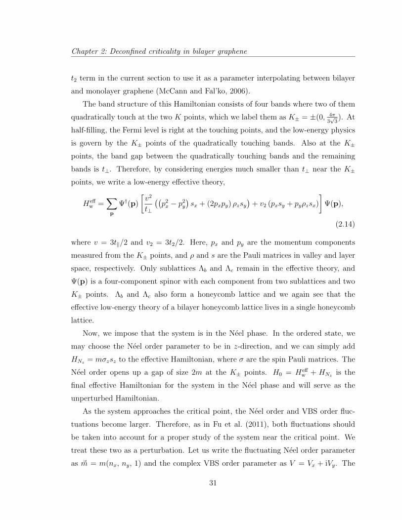
points, we write a low-energy e↵ective theory,
He↵w =
X
p
†(p)v2
t?
��p2x � p2y
�sx + (2pxpy) ⇢zsy
�+ v2 (pxsy + py⇢zsx)
� (p),
(2.14)
where v = 3tk/2 and v2 = 3t2/2. Here, px and py are the momentum components
measured from the K± points, and ⇢ and s are the Pauli matrices in valley and layer
space, respectively. Only sublattices ⇤b and ⇤c remain in the e↵ective theory, and
(p) is a four-component spinor with each component from two sublattices and two
K± points. ⇤b and ⇤c also form a honeycomb lattice and we again see that the
e↵ective low-energy theory of a bilayer honeycomb lattice lives in a single honeycomb
lattice.
Now, we impose that the system is in the Neel phase. In the ordered state, we
may choose the Neel order parameter to be in z-direction, and we can simply add
HNz
= m�zsz to the e↵ective Hamiltonian, where � are the spin Pauli matrices. The
Neel order opens up a gap of size 2m at the K± points. H0 = He↵w + HN
z
is the
final e↵ective Hamiltonian for the system in the Neel phase and will serve as the
unperturbed Hamiltonian.
As the system approaches the critical point, the Neel order and VBS order fluc-
tuations become larger. Therefore, as in Fu et al. (2011), both fluctuations should
be taken into account for a proper study of the system near the critical point. We
treat these two as a perturbation. Let us write the fluctuating Neel order parameter
as ~m = m(nx, ny, 1) and the complex VBS order parameter as V = Vx + iVy. The
31

Chapter 2: Deconfined criticality in bilayer graphene
Hamiltonian of nx, ny is HNxy
= msz (nx�x + ny�y). Recalling that the Kekule type
of bond order can be written as a modulation on the tight binding hopping parameter,
(Hou et al., 2007, 2010)
HV = �X
r2⇤b
3X
i=1
�tr,i c(b)†r c(c)r+s
i
+ h.c., (2.15)
�tr,i = V eiK+·siei(K+�K�)·r/3 + c.c.,
we find HV = �sx (Vx⇢x � Vy⇢y) as the Hamiltonian for the VBS order parameter. So
the perturbation H1 is H1 = HNxy
+HV and now we can write the full Hamiltonian,
H =H0 +H1
=
✓v2
t?
��p2x � p2y
�sx + (2pxpy) ⇢zsy
�+ v2 (pxsy + py⇢zsx) +m�zsz
◆
+ (m (nx�x + ny�y) sz � (Vx⇢x � Vy⇢y) sx) . (2.16)
Note that the terms proportional to the antiferromagnetic order, m, anti-commute
with all the terms in Eq. (2.14), indicating they will open up a gap in the electronic
spectrum. On the other hand, the terms proportional to the VBS order anti-commute
only with the v2 term, but not with the v2/t? term, indicating that VBS order alone
does not open a gap in the purely quadratic-band-touching spectrum.
Writing in a specific basis, †(p) = (c(b)†p+ , c(b)†p� , c(c)†p+ , c(c)†p� ), where ± corresponds
to the K± points the momentum is measured from
H =0
BBBBB@
~m · ~� 0 � v2
t?⇡2 + v2⇡† �Vx � iVy
0 ~m · ~� �Vx + iVy � v2
t?⇡† 2 � v2⇡
� v2
t?⇡† 2 + v2⇡ �Vx � iVy �~m · ~� 0
�Vx + iVy � v2
t?⇡2 � v2⇡† 0 �~m · ~�
1
CCCCCA. (2.17)
Here, ⇡ = ipx + py is defined for notational convenience. Now, it is more apparent
that v2 = 0 gives the Hamiltonian for bilayer graphene and v = 0 gives that of
the monolayer graphene with opposite chirality. Therefore, we may tune v2/v to
interpolate between monolayer and bilayer graphene.
32

Chapter 2: Deconfined criticality in bilayer graphene
Note that the electric field E in Eq. (2.1) is not included in this final form of
the Hamiltonian. However, it is encoded in the order parameters as we have seen
in the previous sections how electric field tunes the Neel to VBS transition. The
electric field has other e↵ects as well, as changing the energy gap of the VBS phase
for example, but this will have only quantitative e↵ects in the calculation. The result
of the calculation with explicit electric field will be presented in the following section.
From Eq. (2.16), we integrate out the fermions to get an e↵ective theory for the
fluctuating order parameters. The coupling between the Neel and VBS order pa-
rameters appears at fourth order of one-loop expansion. For notational simplicity,
we follow Fu et al. (2011) and combine the four real order parameters to a multi-
component bosonic field, Aµ(x, y, ⌧) = (Vx/m, Vy/m, nx, ny). µ = 0, 1, 2, 3 label the
di↵erent fields in Aµ and are not Lorentz indices. In momentum space, the four point
couplings between the bosonic fields are,
S1 =X
µ,⌫,�,�
Z 3Y
i=1
dpiKµ⌫�;�p1p2p3
Aµ(p1)A⌫(p2)A�(p3)
⇥A�(�p1 � p2 � p3). (2.18)
Among this bosonic coupling, we are most interested in the topological term,
Stop = i
Zdxdyd⌧
�KjN⌧ jV⌧ +K 0jNx jVx +K 0jNy jVy
�, (2.19)
which is the coupling term between the skyrmion current jN↵ and VBS current jV� :
jN↵ ⌘ ✏↵��✏abcna@�n
b@�nc,
jV� ⌘ Vx@�Vy � Vy@�Vx. (2.20)
This topological term is of interest to us because it provides an argument that the
system is in VBS phase in the disordered side; as mentioned in the beginning of this
section, this is analogous to arguments in Read and Sachdev (1990) and Fu et al.
(2011).
As explained in detail in Fu et al. (2011), we can extract the couplings K and K 0
33
Chapter 2: Deconfined criticality in bilayer graphene
from Kµ⌫�;�p1p2p3
in Eq. (2.18). The final expression for K is as follows:
8K = K234;1⌧xy +K243;1
⌧yx +K342;1xy⌧ +K324;1
x⌧y +K423;1y⌧x +K432;1
yx⌧
� �K243;1
⌧xy +K234;1⌧yx +K432;1
xy⌧ +K423;1x⌧y +K324;1
y⌧x +K342;1yx⌧
�
� �K134;2
⌧xy +K143;2⌧yx +K341;2
xy⌧ +K314;2x⌧y +K413;2
y⌧x +K431;2yx⌧
�
+K143;2⌧xy +K134;2
⌧yx +K431;2xy⌧ +K413;2
x⌧y +K314;2y⌧x +K341;2
yx⌧ , (2.21)
where K 0 can also be written in a similar way. Here, Kµ⌫�;�↵�� are defined as the
coe�cient of the term linear in p1p2p3:
Kµ⌫�;�p1p2p3
= · · · +Kµ⌫�;�↵�� p↵1p
�2p
�3 + · · · . (2.22)
The lowest order contribution to S1 arises from the one-loop expansion, when we
integrate out the fermion loop. Therefore, the calculation of Kµ⌫�;�↵�� eventually boils
down to calculating box diagrams, as in Fig. 2.5. Note that in Eq. (2.16), the vertex
functions between bosonic fields and fermions have no momentum dependence and
therefore the p↵1 , p�2 , p
�3 dependence comes from the propagator.
After evaluating a number of diagrams and substituting Kµ⌫�;�↵�� ’s to Eq. (2.21) and
its K 0 analog, we obtain the topological couplings K and K 0 of the system. First, we
consider the bilayer limit of v2/v = 0. The integral expressions for K and K 0 are,
K =1
8⇡3
Zdk0dkxdky
8m5t6?v4�k2x + k2
y
��(k2
0 +m2)t2? + (k2x + k2
y)2v4
�4 ,
K 0 =1
8⇡3
Zdk0dkxdky
4m5t6?v4�3(k2
x � k2y)(k
20 +m2)t2? � (k2
x + k2y)
2(13k2x + 3k2
y)v4�
�(k2
0 +m2)t2? + (k2x + k2
y)2v4
�5
=1
8⇡3
Zdk0dkxdky
4m5t6?v4�3(�k2
x + k2y)(k
20 +m2)t2? � (k2
x + k2y)
2(3k2x + 13k2
y)v4�
�(k2
0 +m2)t2? + (k2x + k2
y)2v4
�5 .
(2.23)
The first expression for K 0 is the coupling of jNx jVx and the second is of jNy jVy . They
map to each other by the transformation kx $ ky, which gives the same value when
integrated on a region which has kx $ ky symmetry as well. We can obtain the K
and K 0 of the e↵ective theory by integrating kx and ky in the whole space (Abanov
34

Chapter 2: Deconfined criticality in bilayer graphene
Figure 2.5: The box diagram needed for the calculation of K and K 0. The p↵1p�2p
�3
coe�cient of this box diagram givesKµ⌫�;�↵�� , whichK, K 0 consist of. The exact relation
between K and Kµ⌫�;�↵�� is given in Eq. (2.21). Note that every momentum dependence
comes from the propagator.
and Wiegmann, 2000). In zero temperature, performing the k0, kx, and ky integral
gives K = �1/16⇡ and K 0 = 1/16⇡. This is a quantized value that does not depend
on microscopic parameters m, t?, or v.
Next, we consider the monolayer limit of v2/v � 1. This can be integrated
analytically and gives K = K 0 = 3/32⇡. They are quantized as well as in the bilayer
limit, and the values are consistent with the result from Senthil and Fisher (2006).
We also compute K and K 0 as a function of v2/v and observe how it changes in
the intermediate regime of monolayer and bilayer. The result in Fig. 2.6 shows the
aforementioned limiting values of K = K 0 = 3/32⇡ for monolayer and K = �K 0 =
�1/16⇡ for bilayer, and a continuous interpolation in-between. K and K 0 of the
intermediate regime does not remain quantized, and thus depends on the parameters
of the theory. Through a number of numerical calculations, we observe that the
intermediate values at a given v2/v depend on a single parameter m/t?. Starting
from the bilayer (v2/v = 0), the convergence to the single layer limit occurs more
35

Chapter 2: Deconfined criticality in bilayer graphene
Figure 2.6: The topological couplings K and K 0 as a function of v2/v. We assumetk = t? = m, and the y-axis is in the unit of 1/16⇡. In the bilayer limit of v2/v = 0,the couplings are K = �1/16⇡ and K 0 = 1/16⇡. Both K and K 0 approaches 3/32⇡in the monolayer limit of v2/v � 0.
rapidly for smaller values of m/t?.
The presence of these non-zero terms supports the proposal that the general struc-
ture of the coupling between the Neel and VBS orders is the same as that in the single
layer honeycomb lattice. But the values of the geometric phases di↵er in the weak
coupling theory, although we expect them to coincide in the strong coupling theory
(by the arguments of Read and Sachdev (1990)). This di↵erence suggests that the
weak coupling analysis points to a first-order Neel-VBS transition, while deconfined
criticality is preferred at strong coupling.
2.6 Geometric phases in electric field
We revisit the geometric phase calculation in Sec. 2.5 including the electric field
to the Hamiltonian. As in Eq. (2.26), electric field couples to the layer space as an
36
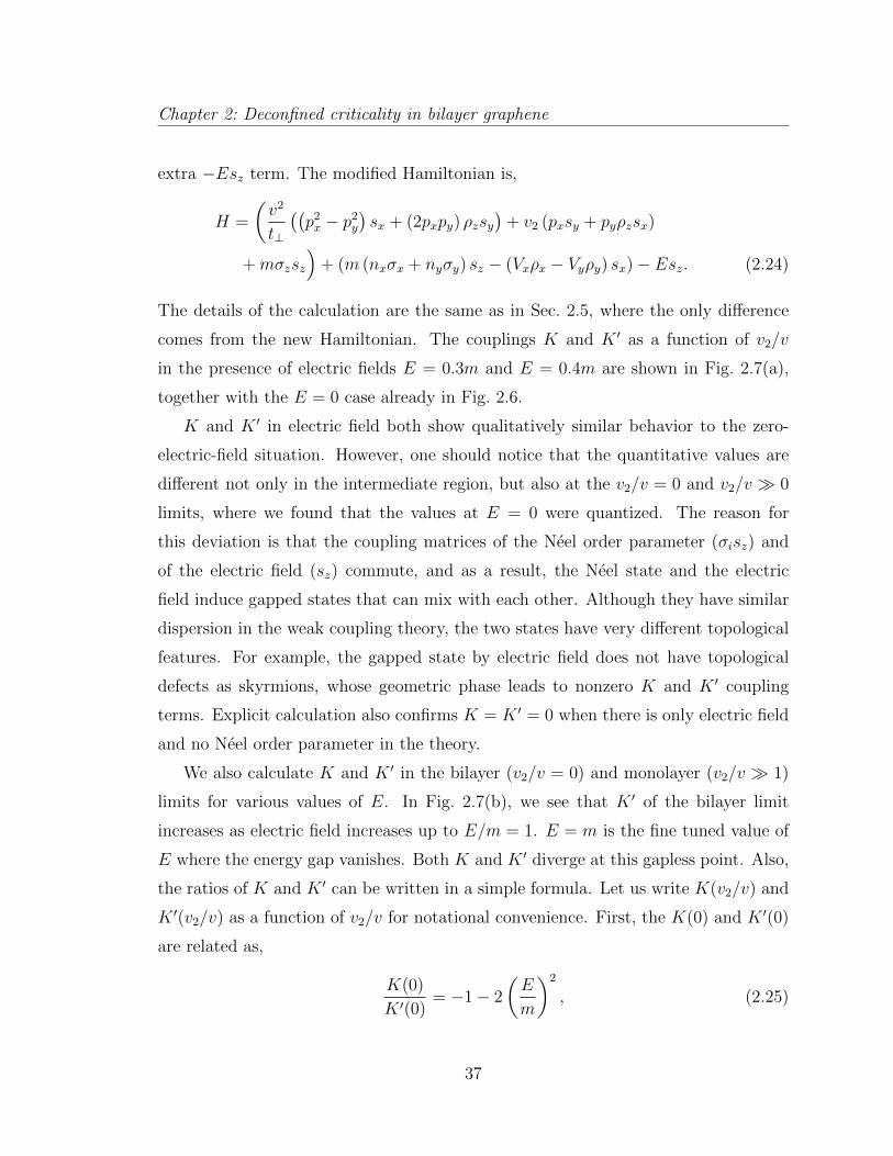
Chapter 2: Deconfined criticality in bilayer graphene
extra �Esz term. The modified Hamiltonian is,
H =
✓v2
t?
��p2x � p2y
�sx + (2pxpy) ⇢zsy
�+ v2 (pxsy + py⇢zsx)
+m�zsz⌘+ (m (nx�x + ny�y) sz � (Vx⇢x � Vy⇢y) sx)� Esz. (2.24)
The details of the calculation are the same as in Sec. 2.5, where the only di↵erence
comes from the new Hamiltonian. The couplings K and K 0 as a function of v2/v
in the presence of electric fields E = 0.3m and E = 0.4m are shown in Fig. 2.7(a),
together with the E = 0 case already in Fig. 2.6.
K and K 0 in electric field both show qualitatively similar behavior to the zero-
electric-field situation. However, one should notice that the quantitative values are
di↵erent not only in the intermediate region, but also at the v2/v = 0 and v2/v � 0
limits, where we found that the values at E = 0 were quantized. The reason for
this deviation is that the coupling matrices of the Neel order parameter (�isz) and
of the electric field (sz) commute, and as a result, the Neel state and the electric
field induce gapped states that can mix with each other. Although they have similar
dispersion in the weak coupling theory, the two states have very di↵erent topological
features. For example, the gapped state by electric field does not have topological
defects as skyrmions, whose geometric phase leads to nonzero K and K 0 coupling
terms. Explicit calculation also confirms K = K 0 = 0 when there is only electric field
and no Neel order parameter in the theory.
We also calculate K and K 0 in the bilayer (v2/v = 0) and monolayer (v2/v � 1)
limits for various values of E. In Fig. 2.7(b), we see that K 0 of the bilayer limit
increases as electric field increases up to E/m = 1. E = m is the fine tuned value of
E where the energy gap vanishes. Both K and K 0 diverge at this gapless point. Also,
the ratios of K and K 0 can be written in a simple formula. Let us write K(v2/v) and
K 0(v2/v) as a function of v2/v for notational convenience. First, the K(0) and K 0(0)
are related as,
K(0)
K 0(0)= �1� 2
✓E
m
◆2
, (2.25)
37
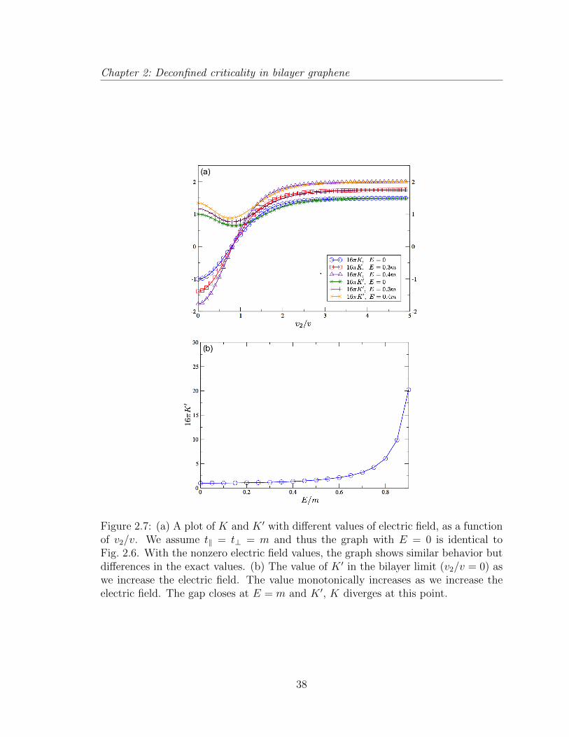
Chapter 2: Deconfined criticality in bilayer graphene
Figure 2.7: (a) A plot of K and K 0 with di↵erent values of electric field, as a functionof v2/v. We assume tk = t? = m and thus the graph with E = 0 is identical toFig. 2.6. With the nonzero electric field values, the graph shows similar behavior butdi↵erences in the exact values. (b) The value of K 0 in the bilayer limit (v2/v = 0) aswe increase the electric field. The value monotonically increases as we increase theelectric field. The gap closes at E = m and K 0, K diverges at this point.
38

Chapter 2: Deconfined criticality in bilayer graphene
when E < m. This gives the correct limiting value for the E = 0 case, where
K(0) = �K 0(0) = �1/16⇡. Also, as one can check roughly in Fig. 2.7(a), K(1) =
K 0(1) = 1.5K 0(0) strictly holds as in the E = 0 limit.
2.7 Zero mode in VBS vortex
Another approach to the theory of deconfined criticality is via the structure of
vortices in the VBS order parameter. Levin and Senthil (2004) presented general
arguments that each such vortex must carry spin S = 1/2. In some case, this fact is
already apparent by the presence of zero modes in a weak coupling theory of the VBS
state: this is the case in monolayer graphene (Hou et al., 2007, 2010). We present a
corresponding computation for the bilayer case, and do not find such zero modes. We
view this as a feature of the weak coupling approach, rather than the inapplicability
of the general strong coupling arguments of Read and Sachdev (1990).
We start in the deep VBS phase and may ignore the Neel order for now. Therefore
we adapt the Hamiltonian (2.16) with m = 0. In this section we return to t2 = 0,
and set the Fermi velocity v = 3tk/2 equal to one. VBS order parameter, V (r) =
Vx(r) + iVy(r), now has a nonzero expectation value, and let us allow it to fluctuate
over space. We will assume the fluctuation is in a much longer length scale than the
lattice constant, which is set to 1, so we can treat the order parameter as a constant
during Fourier transform. Moreover, we include the electric field explicitly as this
will open up an energy gap of the system. The Hamiltonian in the VBS phase is,
H =1
t?
�p2x � p2y
�sx +
1
t?(2pxpy) ⇢zsy
� (Vx(r)⇢x � Vy(r)⇢y) sx � Esz, (2.26)
where ⇢ and s are the Pauli matrices in valley and layer space, respectively. Note that
in the bilayer graphene, the Kekule VBS order does not open up a gap but create
nodal lines which form a circle in the Brillouin zone. The nodal line is protected
by the layer symmetry of the system. Discussing zero modes in a gapless system
is meaningless, however, the transition is at a nonzero electric field. Electric field
39
Chapter 2: Deconfined criticality in bilayer graphene
couples di↵erently with the density of the electrons in di↵erent layers and breaks the
layer symmetry. This opens up a gap at the nodal line and it is now legitimate to
discuss zero modes of the system.
As in Sec. 2.5, choosing a specific basis, †(p) = (c(b)†p+ , c(b)†p� , c(c)†p+ , c(c)†p� ), we can
represent the Hamiltonian as a 4⇥ 4 matrix:
H =
0
BBBBBB@
�E 0 � 1t?⇡2 � V (r)
0 � E � V (r) � 1t?⇡† 2
� 1t?⇡† 2 � V (r) E 0
�V (r) � 1t?⇡2 0 E
1
CCCCCCA. (2.27)
Changing to the real basis, †(r) = (u†b(r), v
†b(r), u
†c(r), v
†c(r)), where for example,
ub(r) =1pN
Pp e
ip·rbp+ and vb(r) =1pN
Pp e
ip·rbp�,
H = � 1
t?
0
BBBBBB@
E 0 4@2z V (r)
0 E V (r) 4@2z
4@2z V (r) � E 0
V (r) 4@2z 0 � E
1
CCCCCCA. (2.28)
Here, we included t? into the definition of V (r) and E for notational convenience and
used a complex coordinate z = x+ iy for 2@z = e�i✓(@r � ir@✓).
Now we assume that the VBS order parameter contains a vortex, V (r) = V0(r)ei✓.
Jackiw and Rossi (1981) provides an analytical method of obtaining the zero modes
when the fermions are Dirac-like. They count the number of zero modes by matching
the two asymptotic behaviors of the solutions of H (r) = 0. The quadratic dis-
persion of fermions can be easily implemented into this scheme, however, including
the electric field ruins the argument and we cannot follow the same step. Alterna-
tively, we have solved the problem numerically. We consider a bilayer honeycomb
lattice with 3600 sites with the corresponding lattice Hamiltonian (2.26), and in-
troduce a vortex at the center of the lattice. Open boundary condition is imposed
to deal with the vortex without including any Dirac strings. Introducing a vortex
and anti-vortex pair will also resolve the issue, but it will also e↵ectively decrease
40
Chapter 2: Deconfined criticality in bilayer graphene
the system size. With the open boundary condition, we turn on a small potential
at the boundary to eliminate zero-energy states arising from boundary e↵ects. We
then numerically diagonalize the system and search for zero-energy eigenvalues. We
also check the eigenfunctions of the states while moving the vortex center around to
confirm whether the wavefunctions are actually localized at the vortex. The result
clearly showed no zero modes in the presence of a vortex. As we noted earlier, we
believe this result is a feature of the weak coupling method, and that the needed zero
mode will appear in the strong coupling limit as argued in Levin and Senthil (2004).
We also mention previous reports about zero modes in vortices of bilayer graphene
(Moon, 2012; Lu and Herbut, 2012). In these works, the authors claim there are two
zero modes for a single vortex of valley ferromagnet order. Note that this order
breaks time reversal symmetry and is di↵erent from the Kekule VBS phase we have
considered above. In the notation of Eq. (2.26), the valley ferromagnet order will be
written as (Vx⇢y + Vy⇢x)sy, which anti-commutes with the kinetic energy terms. Lu
and Herbut (2012) concentrates in regions near the vortex and uses the method of
Jackiw and Rossi (1981) in momentum space. However, this is potentially danger-
ous because, as mentioned before, the number of zero modes is determined by the
matching of the asymptotic behavior of near-vortex and far-vortex regions. Indeed,
without the matching procedure, and only looking in the near-vortex region one can
find an infinite number of zero modes. However, by numerically diagonalizing the
lattice Hamiltonian as above, we indeed find two zero modes for their system with
valley ferromagnet order.
2.8 Conclusions
This chapter has examined the strong coupling limit of an extended Hubbard
model appropriate for undoped bilayer graphene. The results of our analyses are
that the application of a transverse electric field does indeed destabilize the Neel
insulator, and that resulting “quantum disordered” state is likely to have VBS order,
which breaks the space group symmetry of the lattice. These results are in accord with
41

Chapter 2: Deconfined criticality in bilayer graphene
the weak coupling analysis (Kharitonov, 2012b), and our strong coupling arguments
indicate that the Neel-VBS quantum phase transition in bilayer graphene can be in
the deconfined universality class (Senthil et al., 2004a,b).
On the experimental side, there is now good evidence for the Neel state in bilayer
graphene (Maher et al., 2013; Freitag et al., 2013), and also for a quantum transition
out of this state upon application of a transverse electric field (Weitz et al., 2010;
Freitag et al., 2012; Velasco et al., 2012). It would be of great interest to devise
experiments to measure the translational symmetry breaking associated with the VBS
order. The transition to the VBS state should exhibit quantum-critical scaling, and
this may be detected by a careful study of the temperature dependence of the influence
of the transverse electric field on conductance across the transition, and looking for a
“quantum-critical fan” (Sachdev and Keimer, 2011) in the electric-field/temperature
plane.
For experimental applications, the fundamental new idea that a “deconfined-
critical” perspective brings is that the transition out of the Neel state occurs as a
consequence of condensation of low-energy skyrmions in the Neel order (Senthil et al.,
2004a,b); so such low-energy skyrmions should be present in bilayer graphene near
the transition. In the presence of ferromagnetic order, a crucial feature of skyrmions
in the quantum Hall regime is that they carry electric charge (Lee and Kane, 1990;
Sondhi et al., 1993). In the present bilayer case, each layer has intra-layer ferromag-
netism in the Neel state, with opposite orientation in the two layers, and so we can
expect that the layers carry opposite charges in the presence of a skyrmion. With the
application of an electric field, the layer-exchange symmetry is broken, and then a
skyrmion current will carry a net electrical current. It is notable that the experiments
show enhanced conductivity in the region of the transition, (Weitz et al., 2010) and
this could be explained by the presence of low-energy skyrmions in the deconfined-
critical theory. In our present strong-coupling analysis, the orbital magnetic field
e↵ects have been suppressed, and so we have not accounted for the electrical nature
of the skyrmions: an extension of our analysis to include the physics of Landau levels
is required, and is being undertaken. On the experimental side, the opposite layers
42
Chapter 2: Deconfined criticality in bilayer graphene
charges carried by the skyrmion could be studied by driving currents in opposite
directions in the two layers. Also, optical experiments can detect the spin-chirality
fluctuations (Lee and Nagaosa, 1992) linked to the collective gauge excitations of de-
confined criticality; however, it will be necessary for the light to couple selectively to
one layer (i.e., one sublattice of the antiferromagnet).
43

Chapter 3
Wess-Zumino-Witten terms in
graphene Landau levels
3.1 Introduction
A number of recent experimental (Weitz et al., 2010; Freitag et al., 2012; Velasco
et al., 2012; Young et al., 2012; Maher et al., 2013; Freitag et al., 2013; Young et al.,
2014) and theoretical (Herbut, 2007; Jung and MacDonald, 2009; Nandkishore and
Levitov, 2010; Cvetkovic et al., 2012; Zhang et al., 2012; Kharitonov, 2012a,b,c,d;
Lee and Sachdev, 2014; Wu et al., 2014; Dhochak et al., 2015) works have focused
on the presence of antiferromagnetism in neutral monolayer and bilayer graphene
in an applied magnetic field. It has also been argued that a nonmagnetic state
with lattice symmetry breaking in the Kekule valence bond solid (VBS) pattern (see
Fig. 3.1) is proximate to the antiferromagnetic (AF) state (Kharitonov, 2012a,b; Lee
and Sachdev, 2014; Wu et al., 2014). Bilayer graphene o↵ers a particularly attractive
area for studying the interplay between the AF and VBS order because it may be
possible to tune between them by applying a transverse electric field (Weitz et al.,
2010; Kharitonov, 2012b; Lee and Sachdev, 2014).
The presence of the competing AF and VBS orders sets up the possibility (Lee
and Sachdev, 2014) of novel quantum criticality between these orders, similar to
44

Chapter 3: Wess-Zumino-Witten terms in graphene Landau levels
that found in insulating quantum spin models (Read and Sachdev, 1990; Senthil
et al., 2004a,b; Clark et al., 2011; Albuquerque et al., 2011; Ganesh et al., 2013; Zhu
et al., 2013; Block et al., 2013; Gong et al., 2013; Pujari et al., 2013; Lang et al.,
2013). However, these quantum spin models apply in the limit of very large on-site
Coulomb repulsion between the electrons, and this is not the appropriate parameter
regime for graphene. Here we examine a complementary limit of large magnetic
field and moderate interactions, so that it is permissible to project onto an e↵ective
Hamiltonian acting only on the zero energy Landau levels. Such a limit has been
widely used with considerable success in describing the properties of graphene. (Note,
however, that we are still in the regime where the cyclotron gap is still smaller than
the tight-binding hopping parameters, with magnetic fields smaller than 10 T.) Our
main new result is that the Landau level projected e↵ective action for the AF and
VBS orders has a topological Wess-Zumino-Witten (WZW) term (Wess and Zumino,
1971; Witten, 1983; Abanov and Wiegmann, 2000) for both the monolayer and bilayer
cases.
The WZW term has a quantized coe�cient, and it computes a Berry phase linking
together spatial and temporal textures in the AF and VBS orders. It can be viewed
as a higher dimensional generalization of the Berry phase of a single spin S degree
of freedom, which is equal to S times the area enclosed by the spin worldline on the
unit sphere. Similarly, the WZW term here measures the area on the surface of the
sphere in the five-dimensional AF and VBS order parameter space. The presence
of this term implies (Tanaka and Hu, 2005; Senthil and Fisher, 2006; Grover and
Senthil, 2008) that the field theories of deconfined criticality (Senthil et al., 2004a,b)
apply to graphene. Such theories describe the quantum phase transition not in the
conventional Landau terms of fluctuating order parameters, but using fractionalized
degrees of freedom coupled to emergent gauge fields. We will also discuss experimental
implications of these results.
45

Chapter 3: Wess-Zumino-Witten terms in graphene Landau levels
Figure 3.1: AF (left) and Kekule VBS states of bilayer graphene. The blue (red)lines indicate the honeycomb lattice of the top (bottom) layer. The ellipses in theVBS state denote the links between the top and bottom layers which are equivalentlydistorted with respect to the parent lattice.
3.2 Model and results
We begin by directly stating the Hamiltonian of the low energy graphene bands
(see, e.g., Kharitonov (2012d), Lee and Sachdev (2014) for details)
H = v
0 aq
a†q 0
!, (3.1)
where v is a Fermi velocity, a = px � ipy � (e/c)(Ax � iAy) with (px, py) the electron
momentum, (Ax, Ay) is the vector potential of the applied magnetic field, the matrix
acts on the graphene sublattice index, and q = 1 for monolayer graphene, while q = 2
for the bilayer case. For bilayers, the sublattice index coincides with the layer index.
For both monolayers and bilayers, there is an additional twofold valley degeneracy,
along with the usual twofold spin degeneracy (in the absence of a Zeeman coupling).
The a, a† obey commutation relations proportional to those of the ladder operators
of a harmonic oscillator, and so it is easy to diagonalize H. In this manner we obtain
q zero energy Landau levels, which are spanned by the orthonormal eigenfunctions
`(r), where ` = 1, . . . , qN�, with N� the number of flux quanta. So we write the
46
Chapter 3: Wess-Zumino-Witten terms in graphene Landau levels
electron annihilation field operator projected to the zero energy Landau levels as
(r) =qN�X
`=1
`(r)c`, (3.2)
where c` is canonical fermion annihilation operator. In the zero energy Landau levels,
the valley, sublattice, and layer indices all coincide; henceforth we will refer to this as
a valley index, and it can take two values. The fermion operators also carry a spin
index with two possible values, and we do not explicitly display the spin or valley
indices.
We now introduce Pauli matrices �x,y,z which acts on the spin space, and a sec-
ond set ⇢x,y,z which act on the valley space (here we follow the conventions of Lee
and Sachdev (2014)). In terms of these matrices, the three-component AF order
is measured by (⇢z�x, ⇢z�y, ⇢z�z) while the two-component VBS order parameter is
(⇢x, ⇢y).
It is convenient to write the above matrices as
�1 = ⇢z�x , �2 = ⇢z�y , �3 = ⇢z�z , �4 = ⇢x , �5 = ⇢y
and to notice that the 5 �a matrices anticommute and square to unity; indeed these
are the 5 Dirac gamma matrices. Their 10 products i�a�b (a 6= b) realize the Lie
algebra of SO(5), and the 15 matrices �a and i�a�b realize the Lie algebra of SU(4).
Next, we introduce a five-component unit vector na(r, ⌧), where r = (x, y) are
the spatial coordinates and ⌧ is imaginary time, representing the combined spacetime
fluctuations of the AF and VBS orders. Then the imaginary time Lagrangian of the
electrons projected to the zero energy Landau levels is
L =qN�X
`=1
c†`@c`@⌧� �
Zd2r na(r, ⌧)
†(r, ⌧)�a (r, ⌧) , (3.3)
where � is the coupling of the electrons to the AF and VBS orders, and there is an
implicit sum of a over five values, and also over the spin and valley indices. The � term
arises from a decoupling of the electron-electron interactions specified in Kharitonov
(2012a), Lee and Sachdev (2014), and Wu et al. (2014).
47
Chapter 3: Wess-Zumino-Witten terms in graphene Landau levels
Now we can state our primary result. We integrate over the the c` electrons in Land obtain an e↵ective action for unit vector na(r, ⌧). Apart from the usual terms
of the O(5) nonlinear sigma model considered in Wu et al. (2014) (and anisotropies
due to the Zeeman coupling, electron-electron interactions, and a possible transverse
electric field for bilayers), the e↵ective action has a topological WZW term at level q,
SWZW = 2⇡iq W [na], (3.4)
W [na] =3
8⇡2
Z 1
0
du
Zd2rd⌧✏abcdena@xnb@ync@⌧nd@une.
Here we have introduced the extra coordinate u, and na(r, ⌧, u) is any function which
smoothly extrapolates from the physical na(r, ⌧) at u = 1 to a fixed value (say)
na = (1, 0, 0, 0, 0) at u = 0. The choice of the extrapolation can only change W [na]
by integers, and so e2⇡iqW is well defined.
In the case of graphene in zero magnetic field and weak interactions, the same
WZW term between the Neel and VBS orders is also present (Fu et al., 2011). How-
ever, for the experimentally important case of bilayer graphene, there is no such WZW
term for the AF and VBS orders at zero field and weak interactions (Moon, 2012; Lee
and Sachdev, 2014) (although, E.-G. Moon has noted such a term for the quantum
spin Hall order (Moon, 2012)); so, in this case the zero energy Landau level projection
is crucial for obtaining the topological coupling.
Such a WZW term has a strong impact in the interplay between the order param-
eters. As we will review below, it topologically links AF order to defects of the VBS
order, and vice versa.
3.3 Derivation
We provide two derivations of Eq. (3.4).
First, pick any three of the five na components, say a = u, v, w, and set the other
two to zero. Then we have unit 3-vector field ~N = (nu, nv, nw). Now consider a static
Skyrmion texture in ~N(r). Then by a computation parallel to that in Section III.B
of Moon et al. (1995) (and its generalization to q = 2 (Abanin et al., 2009)), the
48

Chapter 3: Wess-Zumino-Witten terms in graphene Landau levels
Skyrmion acquires a “charge.” In the present situation the charge is measured by
i�u�v�w and its spatial density is
⌦ †(r) i�u�v�w (r)
↵=
q
2⇡~N · (@x ~N ⇥ @y ~N), (3.5)
where the angular brackets represent the expectation value over the occupied states
in the zero energy Landau level perturbed by the texture in ~N as in L. (A similar
relationship has been noted in monolayer graphene in zero magnetic field from Herbut
et al. (2012); however, no such relationship applies to bilayer graphene in zero field.)
A detailed derivation of Eq. (3.5) is provided in the next paragraph. Now consider a
VBS vortex, i.e., a 2⇡ vortex in (n4, n5) applied to L. For a two-component order, the
core of the vortex has a singularity, but this can be relieved by orienting na in a third
direction, say (±1, 0, 0, 0, 0). Now the VBS vortex is equivalent to a half-Skyrmion
in ~N = (n1, n4, n5), and after integrating Eq. (3.5) over all space, this vortex has
h�xi = ±q. Similarly, vortex cores in the directions (0,±1, 0, 0, 0) and (0, 0,±1, 0, 0)
yield h�yi = ±q and h�zi = ±q. So we reach the important conclusion that the VBS
vortex has total spin S = q/2, and has an associated (q + 1)-fold degeneracy. For
q = 1, note that this is precisely the situation considered in Levin and Senthil (2004)
for quantum spin models (see also Hou et al. (2010)). Alternatively, we can examine
the fate of SWZW in the presence of such VBS vortices: following a computation by
Grover and Senthil (Grover and Senthil, 2008), we find that the WZW term reduces
to the quantum Berry phase of a single spin with S = q/2. From this we conclude
that Eq. (3.5) implies Eq. (3.4).
Now we give a detailed derivation of Eq. (3.5). We work in Landau gauge and
separate the quantum number l in Eq. (3.2) into n and X, where n is the Landau level
index and X is the center of the magnetic oscillator. Recall for monolayer graphene
(q = 1) n is 0, and for bilayer graphene (q = 2) n is over 0 and 1. There are N� of X
labels, so the total number of states in the zero energy Landau level is qN�.
The spatial wavefunction n,X(r) in Eq. (3.2) is:
n,X(r) = eiXy'n,X(x), (3.6)
49

Chapter 3: Wess-Zumino-Witten terms in graphene Landau levels
where 'n,X(x) are the n-th harmonic oscillator eigenfunction:
'0,X(x) =1
⇡1/4e�(x�X)2/2,
'1,X(x) =
p2(x�X)
⇡1/4e�(x�X)2/2. (3.7)
Note that we work in the unit where the magnetic length lB = 1. We also set the
volume of the system as 1 to avoid volume factors in Fourier transform.
Now we can write the Hamiltonian in cn,X basis.
H = ��Z
d2r na(r) †(r)�a (r)
= ��Z
d2r d2q e�iq·rna(�q)X
n,X,n0,X0
c†n,X'n,X(x)e�iXy �a e
iX0y'n0,X0(x)cn0,X0
= ��Z
d2q na(�q)X
n,n0,X
e�iqx
Xc†n,X�qy
/2 �a cn0,X+qy
/2Fn,n0(q) (3.8)
The form factors Fn,n0(q) are calculated as,
F00(q) = e�q2/4,
F01(q) =(�iqx � qy)p
2e�q2/4,
F10(q) =(�iqx + qy)p
2e�q2/4,
F11(q) = (1� q2/2)e�q2/4. (3.9)
The di↵erence in Eq. (3.8) between q = 1 and q = 2 case comes from the summation
limit of n and n0.
Let us define the operator Oa(q) to be the last part of Eq. (3.8),
Oa(q) =X
n,n0,X
e�iqx
Xc†n,X�qy
/2 �a cn0,X+qy
/2Fn,n0(q). (3.10)
We can calculate the commutator of two Oa operators to the lowest order in momen-
50
Chapter 3: Wess-Zumino-Witten terms in graphene Landau levels
tum. In this derivation, we concentrate on the case of bilayer graphene, q = 2.
[Oa(q),Ob(k)]
=X
n,n0,m,Z
e�i(qx
+kx
)Zei(qxky�qy
kx
)/2Fnm(q)Fmn0(k)c†n,Z�(qy
+ky
)/2 �a�b cn0,Z+(qy
+ky
)/2
� (q $ k, a$ b)
=X
Z
e�i(qx
+kx
)Zc†1,Z�(qy
+ky
)/2
✓�a�b + �b�a
2
◆c1,Z+(q
y
+ky
)/2
⇥ �2i(kyqx � kxqy) + O(q,k)2
�
+X
n,Z
e�i(qx
+kx
)Zc†n,Z�(qy
+ky
)/2
✓�a�b � �b�a
2
◆cn,Z+(q
y
+ky
)/2 ⇥ (2 + O(q,k))
(3.11)
For the 3-vector field ~N(r) defined previously, we assume nw ! 1 as r !1, i.e.,
~N(r ! 1) = (0, 0, 1) ⌘ ~N0. This choice is arbitrary and may be rotated by any
SO(3) transformation. If we denote |GSi to be the ground state with ~N(r) = ~N0,
the expectation value of †(r)�w (r) will be,
hGS| †(r)�w (r)|GSi = 4
2⇡. (3.12)
We impose a Skyrmion texture to the ground state by rotating the spinors by an
operator O,
O =X
r
~⌦(r) · †(r)
~�
2 (r)
!
=X
q
~⌦(�q)2
~ON(q), (3.13)
where ~⌦(r) = ~N0 ⇥ ~N(r), ~� = (�u,�v,�w), and ~ON = (Ou,Ov,Ow). The Skyrmion
state is now e�iO|GSi. Let us also define the Fourier transform of the operator
†(r)i�u�v�w (r) to be O�(k).
Now we follow the derivation from Moon et al. (1995).
hO�(k)i = hGS|eiOO�(k)e�iO|GSi � hGS|O�(k)|GSi
= ihGS|[O,O�(k)]|GSi � 1
2hGS| [O, [O,O�(k)]] |GSi+ · · · (3.14)
51
Chapter 3: Wess-Zumino-Witten terms in graphene Landau levels
The first term vanishes and we ignore the higher order terms in O since we consider a
smooth texture. The derivation boils down to calculating the ground state expectation
value of [O, [O,O�(k)]].
First, we compute [O,O�(k)] using Eq. (3.11).
[O,O�(k)] =X
q
⌦a(�q)2
[OaN(q),O�(k)]
=X
q
⌦a(�q)2
(�kyqx + kxqy) ✏acd
⇥X
Z
e�i(qx
+kx
)Zc†1,Z�(qy
+ky
)/2 �c�d c1,Z+(qy
+ky
)/2. (3.15)
a = u, v, w is the vector index and repeated indices are summed implicitly. Since
[�a,�u�v�w] = 0 for all a, we considered only the symmetric term in Eq. (3.11). The
anti-symmetric tensor is ordered as ✏uvw = 1.
Now we calculate [O, [O,O�(k)]].
[O, [O,O�(k)]] =X
p
⌦b(�p)2
⇥ObN(p), [O,O�(k)]
⇤
=X
p,q
⌦a(�q)⌦b(�p)4
(�kyqx + kxqy) ✏acd
⇥"X
n,n0,X
e�ipx
Xc†n,X�py
/2 �b cn0,X+py
/2Fn,n0(p),
X
Z
e�i(qx
+kx
)Zc†1,Z�(qy
+ky
)/2 �c�d c1,Z+(qy
+ky
)/2
#(3.16)
We have assumed the ground state is uniform, ~N(r) = ~N0. Therefore, the expectation
value of the above expression is nonzero only when �p = q+k. When this condition is
satisfied, the last commutator simplifies toP
Z c†1,Z [�b,�c�d]c1,Z , to the lowest order of
52
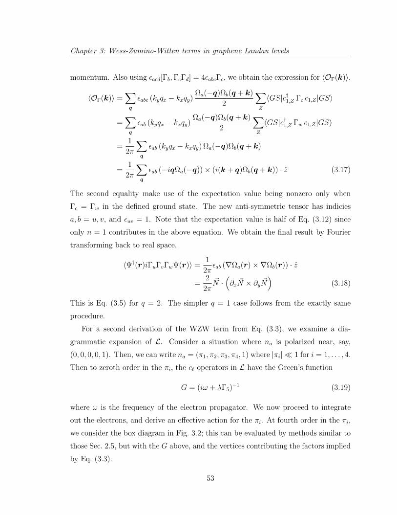
Chapter 3: Wess-Zumino-Witten terms in graphene Landau levels
momentum. Also using ✏acd[�b,�c�d] = 4✏abc�c, we obtain the expression for hO�(k)i.
hO�(k)i =X
q
✏abc (kyqx � kxqy)⌦a(�q)⌦b(q + k)
2
X
Z
hGS|c†1,Z �c c1,Z |GSi
=X
q
✏ab (kyqx � kxqy)⌦a(�q)⌦b(q + k)
2
X
Z
hGS|c†1,Z �w c1,Z |GSi
=1
2⇡
X
q
✏ab (kyqx � kxqy)⌦a(�q)⌦b(q + k)
=1
2⇡
X
q
✏ab (�iq⌦a(�q))⇥ (i(k + q)⌦b(q + k)) · z (3.17)
The second equality make use of the expectation value being nonzero only when
�c = �w in the defined ground state. The new anti-symmetric tensor has indicies
a, b = u, v, and ✏uv = 1. Note that the expectation value is half of Eq. (3.12) since
only n = 1 contributes in the above equation. We obtain the final result by Fourier
transforming back to real space.
h †(r)i�u�v�w (r)i = 1
2⇡✏ab (r⌦a(r)⇥r⌦b(r)) · z
=2
2⇡~N ·
⇣@x ~N ⇥ @y ~N
⌘(3.18)
This is Eq. (3.5) for q = 2. The simpler q = 1 case follows from the exactly same
procedure.
For a second derivation of the WZW term from Eq. (3.3), we examine a dia-
grammatic expansion of L. Consider a situation where na is polarized near, say,
(0, 0, 0, 0, 1). Then, we can write na = (⇡1, ⇡2, ⇡3, ⇡4, 1) where |⇡i|⌧ 1 for i = 1, . . . , 4.
Then to zeroth order in the ⇡i, the c` operators in L have the Green’s function
G = (i! + ��5)�1 (3.19)
where ! is the frequency of the electron propagator. We now proceed to integrate
out the electrons, and derive an e↵ective action for the ⇡i. At fourth order in the ⇡i,
we consider the box diagram in Fig. 3.2; this can be evaluated by methods similar to
those Sec. 2.5, but with the G above, and the vertices contributing the factors implied
by Eq. (3.3).
53
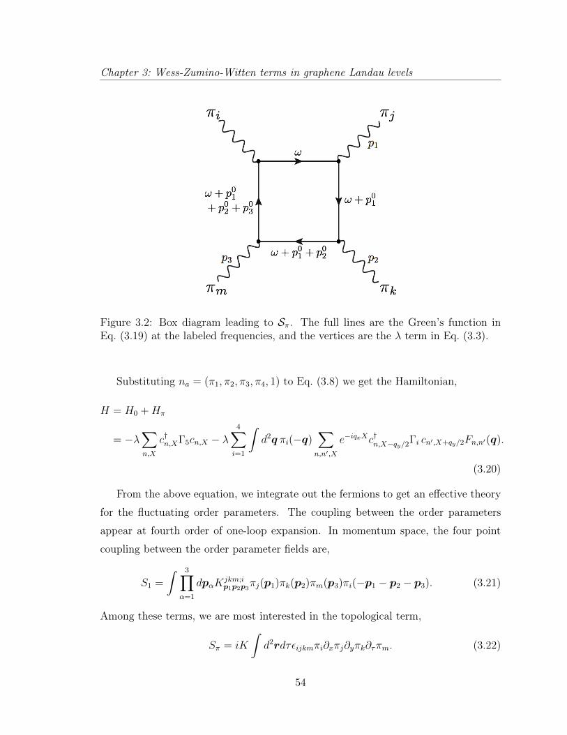
Chapter 3: Wess-Zumino-Witten terms in graphene Landau levels
Figure 3.2: Box diagram leading to S⇡. The full lines are the Green’s function inEq. (3.19) at the labeled frequencies, and the vertices are the � term in Eq. (3.3).
Substituting na = (⇡1, ⇡2, ⇡3, ⇡4, 1) to Eq. (3.8) we get the Hamiltonian,
H = H0 +H⇡
= ��X
n,X
c†n,X�5cn,X � �4X
i=1
Zd2q ⇡i(�q)
X
n,n0,X
e�iqx
Xc†n,X�qy
/2�i cn0,X+qy
/2Fn,n0(q).
(3.20)
From the above equation, we integrate out the fermions to get an e↵ective theory
for the fluctuating order parameters. The coupling between the order parameters
appear at fourth order of one-loop expansion. In momentum space, the four point
coupling between the order parameter fields are,
S1 =
Z 3Y
↵=1
dp↵Kjkm;ip1p2p3
⇡j(p1)⇡k(p2)⇡m(p3)⇡i(�p1 � p2 � p3). (3.21)
Among these terms, we are most interested in the topological term,
S⇡ = iK
Zd2rd⌧✏ijkm⇡i@x⇡j@y⇡k@⌧⇡m. (3.22)
54

Chapter 3: Wess-Zumino-Witten terms in graphene Landau levels
To extract the coe�cient K from S1 we expand Kjkm;ip1p2p3
in powers of momenta
and frequency, and consider the terms linear in p1p2p3:
Kjkm;ip1p2p3
= · · · +Kjkm;i↵�� p↵1p
�2p
�3 + · · · . (3.23)
Here, ↵, �, � are spacetime indices ⌧, x, y. In real space, these terms correspond to
the derivative expansion.
S1 = · · · + i4X
i,j,k,m=1
Kjkm;i↵��
Zd2rd⌧⇡i@↵⇡j@�⇡k@�⇡m + · · · . (3.24)
Comparing Eq. (3.22) with Eq. (3.24), we obtain the expression for K in terms of
Kjkm;i↵�� ’s.
24K = ✏↵��✏ijkmKjkm;i↵�� . (3.25)
Note the summation of repeated indices are implicit, and thus the right-hand side of
the above equation consists of 144 terms.
Now we only need to calculateKjkm;i↵�� to obtainK. This can be done by calculating
the box diagrams in Fig. 3.2. The kinetic energy of fermions are quenched, and
the propagators are momentum independent. Therefore, the momentum dependence
comes from the vertices and frequency dependence comes from the propagator.
Recalling Eq. (3.20), the inverse Green’s function is written as G�1 = �i! +H0,
where ! is the Matsubara frequency of the fermions. The e↵ective action of order ⇡4
in perturbation theory, which is of our interest according to Eq. (3.24), is:
S[⇡4] =1
4tr (GH⇡GH⇡GH⇡GH⇡) . (3.26)
Considering the momentum flow in Fig. 3.2, we obtain the expression for Kjkm;i↵�� .
Kjkm;i↵�� =
1
4
⇣@p↵1 @p�2
@p�3 tr�G(k)Hj
⇡(p1)G(k + p1)Hk⇡(p2)G(k + p1 + p2)
⇥Hm⇡ (p3)G(k + p1 + p2 + p3)H
i⇡(�p1 � p2 � p3)
����p1=p2=p3=0
.
(3.27)
We used a shorthand notation Ha⇡ for Ha
⇡ = H⇡(⇡i=a = 1, ⇡i 6=a = 0).
55

Chapter 3: Wess-Zumino-Witten terms in graphene Landau levels
We get the value of K by calculating Eq. (3.27). In zero temperature, the fre-
quency integral can be done analytically,
K =1
2⇡
Zd!
X
X
2q�5
(!2 + �2)3
=X
X
3q
8
=3q
16⇡. (3.28)
The individual diagram is independent of X, merely reflecting momentum conser-
vation. Therefore the X summation is just multiplying N�, which equals (sample
area)/(2⇡). This yields the following contribution to the action:
S⇡ =i3q
16⇡
Zd2rd⌧✏ijkm⇡i@x⇡j@y⇡k@⌧⇡m . (3.29)
It can be checked that Eq. (3.4) reduces to S⇡ for na = (⇡1, ⇡2, ⇡3, ⇡4, 1), and so SWZW
is the explicitly SO(5) invariant form of S⇡.
3.4 Theoretical consequences
We now turn to a discussion of the theoretical consequences of the WZW term for
the vicinity of the AF-VBS transition. For q = 1, it has been demonstrated in Levin
and Senthil (2004), Grover and Senthil (2008), Senthil and Fisher (2006) that the
O(5) nonlinear sigma model with O(3)⇥O(2) anisotropy and a level 1 WZW term is
equivalent to the CP1 model in 2+1 dimensions. This is the same model appearing in
the AF-VBS transition of SU(2) quantum spin models (Senthil et al., 2004a,b), and is
a relativistic field theory with a U(1) gauge field and a two-component complex scalar
z↵. In terms of these fields, the AF order is z⇤↵�s↵�z�, with s = x, y, z; so the vector
AF order has been “fractionalized” into spinons z↵. Alternatively, we can also view
the z↵ quanta as representing the vortices or antivortices in the VBS order (Levin
and Senthil, 2004) which, as we have just seen, carry spin S = 1/2.
Presently, the experimentally accessible case of the AF-VBS transition is in bilayer
graphene, so we focus now on the q = 2 case. With a level 2 WZW term, the VBS
56

Chapter 3: Wess-Zumino-Witten terms in graphene Landau levels
vortices carry spin S = 1, and therefore we need complex scalar fields with three
components: we write these as Zs, with s = x, y, z. The field theory of the Zs
quanta is now the CP2 model with anisotropic quartic terms; such a field theory was
considered in Grover and Senthil (2007) in a di↵erent context:
Lcp = |(@µ � iAµ)Zs|2 + g|Zs|2 + u1(|Zs|2)2 + u2(Z2s )(Z
⇤2t ).
Here µ is a spacetime index, Aµ is the emergent U(1) gauge field, g is the coupling
which tunes the AF to VBS transition, and u1,2 are quartic couplings. In terms of the
degrees of freedom in Lcp, the three-component AF order parameter is now i✏stuZ⇤t Zu,
while the complex VBS order h⇢x + i⇢yi ⇠ ei✓ is the monopole operator in the U(1)
gauge field (Read and Sachdev, 1990; Senthil et al., 2004b).
For both the CP1 and CP2 models mentioned above, both first and second order
transitions are possible between the AF and VBS states. A recent numerical study
(Wu et al., 2014) on a single layer model indicates a first order transition for the
parameters studied.
3.5 Experimental implications
Finally, we turn to experimental consequences for bilayer graphene. The defining
characteristic of deconfined criticality is the presence of a gapless “photon” excitation
of an emergent U(1) gauge field (Senthil et al., 2004a). This is associated with the Aµ
above, and can also be interpreted as a “spin-wave” excitation involving fluctuations
of the angle ✓. Our definition of ✓ shows that it is the angular phase associated
with o↵-diagonal-long-range order (ODLRO) in valley space. The valley anisotropy
terms in graphene are very small (Kharitonov, 2012a; Wu et al., 2014), because it is
suppressed by powers of the lattice spacing to the magnetic length; so we expect a
nearly gapless ✓ spin-wave mode to be present (and most of the remarks below to
also apply) even in the case of a first-order transition.
Now recall the fact, noted earlier, that in the zero energy Landau levels the valley
index coincides with the layer index of bilayer graphene (and also the sublattice
57

Chapter 3: Wess-Zumino-Witten terms in graphene Landau levels
index). So ODLRO in valley space is accompanied by ODLRO in the layer space;
i.e., ✓ is also the angular phase of interlayer excitonic superfluidity. Signatures of
excitonic superfluidity have been observed in quantum Hall states in GaAs bilayers
(Eisenstein, 2014). However, in the GaAs bilayers there is negligible tunneling of
electrons between the layers, and this crucial to the emergence of a U(1) symmetry
which is broken by the excitonic condensate. So it might seem surprising that a
similar superfluidity can be present in graphene bilayers, in the presence of very
strong tunneling between the layers. The resolution is the identification of the layer
and valley indices in the zero energy Landau levels of bilayer graphene: in the absence
of intervalley scattering by impurities, and the irrelevancy of valley anisotropy terms
to be presented below, there is also an emergent interlayer U(1) symmetry in bilayer
graphene.
The counterflow electrical current can be written in terms of the gauge field
Jtµ � Jbµ =4e
2⇡✏µ⌫�@⌫A� (3.30)
where Jt and Jb are the currents in the top and bottom layers, and e is the charge
of the electron. The factor of 4 is deduced from Eq. (3.5), which shows that a
AF Skyrmion in (n1, n2, n3) has excitonic charge density h⇢zi = 4 for q = 2. The
counterflow conductivity can be computed from Eq. (3.30) using Lcp; at the g = gc
deconfined quantum critical point this implies a universal value of order, the quantum
unit of conductance e2/h.
For g > gc, in the VBS state, the conductivity should be computed using an
e↵ective action for ✓ which includes the influence of monopoles. Now the current is
Jtµ � Jbµ = 4e⇢s@µ✓ (3.31)
where ⇢s is the sti↵ness of the excitonic superfluidity appearing the e↵ective La-
grangian density
L✓ =⇢s2(@µ✓)
2 � y3 cos(3✓), (3.32)
with y3 the fugacity of tripled monopoles which are allowed by the threefold rotational
symmetry of the underlying honeycomb lattice (Read and Sachdev, 1990). The sti↵-
ness vanishes as ⇢s ⇠ (g � gc)⌫ by the Josephson relation, where ⌫ is the correlation
58

Chapter 3: Wess-Zumino-Witten terms in graphene Landau levels
length exponent. Away from the critical point, the bare value y03 is proportional to
the very small threefold valley anisotropy term (Kharitonov, 2012a; Wu et al., 2014);
y3 has a further suppression (Chubukov et al., 1994; Senthil et al., 2004b) from the
critical fluctuations of Lcp leading to y3 = y03(g � gc)⌫�, where � is the scaling di-
mension of the tripled monopole operator. So the e↵ective “interlayer tunneling”
term, y3, is highly suppressed near the deconfined quantum critical point. We also
note that numerical studies on square lattice antiferromagnets have provided strik-
ing evidence for the emergent U(1) symmetry due to the suppression of monopoles
(Sandvik, 2007), and there is direct evidence for the suppression of monopoles on the
honeycomb lattice in the work of Block et al. (2013).
In GaAs bilayers (Eisenstein, 2014), the excitonic superfluidity is most directly
observed in counterflow experiments, where electric currents flow in the opposite di-
rection in the two layers. This would be technically more di�cult in bilayer graphene,
given the close spacing of the layers, but experiments of this type would be ideal. In
the bilayer graphene experiments of Weitz et al. (2010), there is a Zeeman coupling
to the magnetic field (whose consequences have been studied earlier in Senthil et al.
(2004b)), and an electric field is applied transverse to the layers. The electric field
provides a small breaking of the layer-exchange symmetry. In the presence of such
a symmetry breaking, there is a coupling between the counterflow and parallel cur-
rent modes, and a vestige of the counterflow superfluidity would also be present in a
measurement of the total current in both layers. Weitz et al. (2010) observe a phase
transition out of the (presumed) AF state, signaled by the enhancement of the con-
ductivity. We propose that this enhancement is due to the coupling to counterflow
superfluidity.
59
Chapter 4
Electronic quasiparticles in the
quantum dimer model:
density matrix renormalization
group results
4.1 Introduction
A recent paper (Punk et al., 2015) has proposed a simple quantum dimer model
for the pseudogap metal state of the hole-doped cuprates. The objective of this model
is to describe a metal with electron-like quasiparticles, carrying spin 1/2 and charge
e, but with a Fermi volume which violates the Luttinger theorem for a Fermi liquid
(FL). In particular, doping a density of p holes away from a half-filled insulator should
yield, in Fermi liquid theory, a hole Fermi surface of size 1+ p. And indeed, just such
a Fermi surface is observed at large p (Plate et al., 2005). However, for p ⇡ 0.1,
in the pseudogap metals, many physical properties are well described by a model of
electron-like quasiparticles with a Fermi surface of size p (Sachdev and Chowdhury,
2016). Such a Fermi surface can be obtained in a ‘fractionalized Fermi liquid’ (FL*)
(Senthil et al., 2003, 2004). The model of Punk et al. (2015) was designed to yield a
60
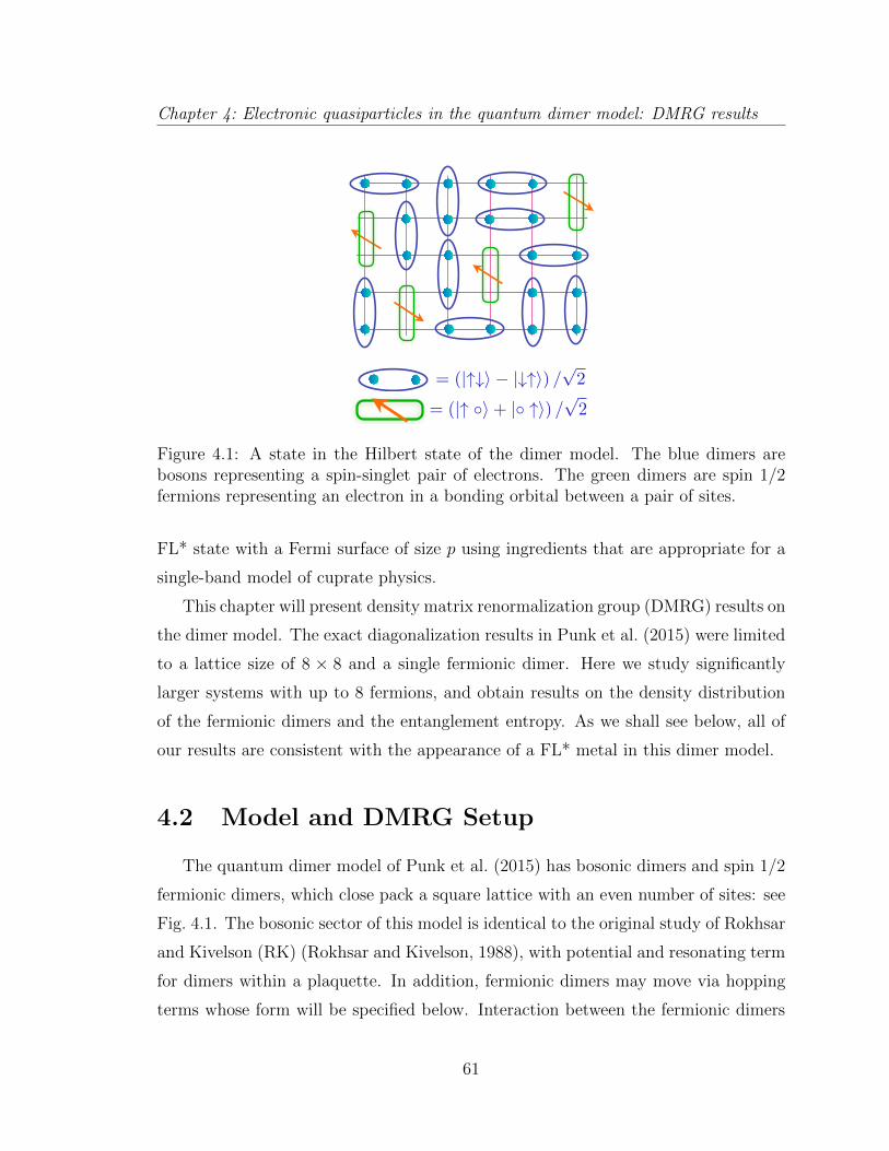
Chapter 4: Electronic quasiparticles in the quantum dimer model: DMRG results
= (|" �i + |� "i) /p
2
= (|"#i � |#"i) /p
2
Figure 4.1: A state in the Hilbert state of the dimer model. The blue dimers arebosons representing a spin-singlet pair of electrons. The green dimers are spin 1/2fermions representing an electron in a bonding orbital between a pair of sites.
FL* state with a Fermi surface of size p using ingredients that are appropriate for a
single-band model of cuprate physics.
This chapter will present density matrix renormalization group (DMRG) results on
the dimer model. The exact diagonalization results in Punk et al. (2015) were limited
to a lattice size of 8 ⇥ 8 and a single fermionic dimer. Here we study significantly
larger systems with up to 8 fermions, and obtain results on the density distribution
of the fermionic dimers and the entanglement entropy. As we shall see below, all of
our results are consistent with the appearance of a FL* metal in this dimer model.
4.2 Model and DMRG Setup
The quantum dimer model of Punk et al. (2015) has bosonic dimers and spin 1/2
fermionic dimers, which close pack a square lattice with an even number of sites: see
Fig. 4.1. The bosonic sector of this model is identical to the original study of Rokhsar
and Kivelson (RK) (Rokhsar and Kivelson, 1988), with potential and resonating term
for dimers within a plaquette. In addition, fermionic dimers may move via hopping
terms whose form will be specified below. Interaction between the fermionic dimers
61
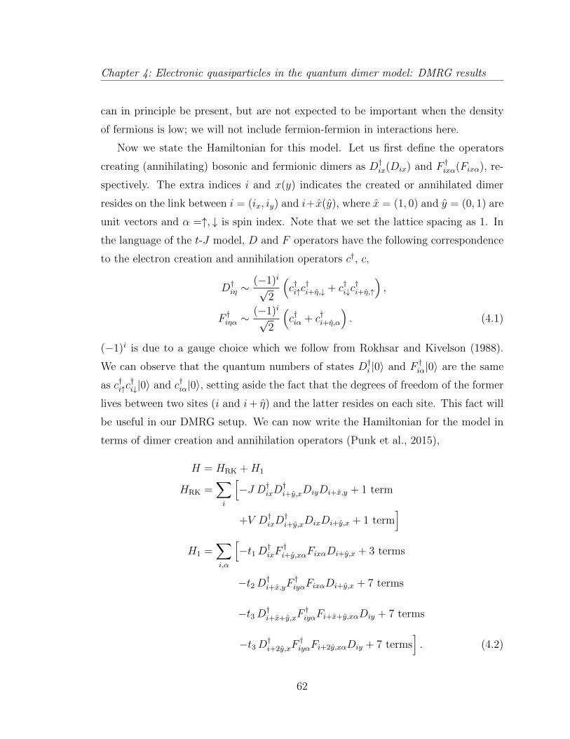
Chapter 4: Electronic quasiparticles in the quantum dimer model: DMRG results
can in principle be present, but are not expected to be important when the density
of fermions is low; we will not include fermion-fermion in interactions here.
Now we state the Hamiltonian for this model. Let us first define the operators
creating (annihilating) bosonic and fermionic dimers as D†ix(Dix) and F †
ix↵(Fix↵), re-
spectively. The extra indices i and x(y) indicates the created or annihilated dimer
resides on the link between i = (ix, iy) and i+x(y), where x = (1, 0) and y = (0, 1) are
unit vectors and ↵ =", # is spin index. Note that we set the lattice spacing as 1. In
the language of the t-J model, D and F operators have the following correspondence
to the electron creation and annihilation operators c†, c,
D†i⌘ ⇠
(�1)ip2
⇣c†i"c
†i+⌘,# + c†i#c
†i+⌘,"
⌘,
F †i⌘↵ ⇠
(�1)ip2
⇣c†i↵ + c†i+⌘,↵
⌘. (4.1)
(�1)i is due to a gauge choice which we follow from Rokhsar and Kivelson (1988).
We can observe that the quantum numbers of states D†i |0i and F †
i↵|0i are the same
as c†i"c†i#|0i and c†i↵|0i, setting aside the fact that the degrees of freedom of the former
lives between two sites (i and i+ ⌘) and the latter resides on each site. This fact will
be useful in our DMRG setup. We can now write the Hamiltonian for the model in
terms of dimer creation and annihilation operators (Punk et al., 2015),
H = HRK +H1
HRK =X
i
h�J D†
ixD†i+y,xDiyDi+x,y + 1 term
+V D†ixD
†i+y,xDixDi+y,x + 1 term
i
H1 =X
i,↵
h�t1 D†
ixF†i+y,x↵Fix↵Di+y,x + 3 terms
�t2 D†i+x,yF
†iy↵Fix↵Di+y,x + 7 terms
�t3 D†i+x+y,xF
†iy↵Fi+x+y,x↵Diy + 7 terms
�t3 D†i+2y,xF
†iy↵Fi+2y,x↵Diy + 7 terms
i. (4.2)
62
Chapter 4: Electronic quasiparticles in the quantum dimer model: DMRG results
The terms we have not explicitly written down are connected with the previous term
through a symmetry transformation of the square lattice. HRK is the pure bosonic
sector mentioned above; J is the coupling for the resonant term, and V is the coupling
for the potential term. H1 contains the hopping terms of the fermionic dimers; t1, t2,
and t3 correspond to three distinct types of hoppings.
In our DMRG calculation, we consider a lattice with geometry of a finite cylinder.
The circumference of the cylinder consists of four lattice sites, and the length of
the cylinder is up to 32 sites. In the second part of this chapter, we also compute
entanglement entropies in 64 ⇥ 2 cylinder to observe one-dimensional e↵ects. We
repeat our calculation in di↵erent fermionic dimer densities, from one to 8 fermionic
dimers. Note that in our lattice configuration, 8 fermionic dimers correspond to 1/16
doping in the typical cuprate phase diagram. We use two sets of parameters for
the couplings in Eq. (4.2). One is the parameters which is relevant to the physical
model for the cuprates in the pseudogap regime: t1 = �1.05J , t2 = 1.95J , and
t3 = �0.6J , at the RK point (J = V ). The other is the parameter which we choose
for comparison: t1 = t2 = t3 = J , at the RK point (J = V ). Single fermion
study in Punk et al. (2015) suggests the di↵erent hopping parameters change the
dispersion of the fermionic dimer: the Fermi surface consists of four hole pockets near
(±⇡/2, ±⇡/2) in the former parameter regime, and a single Fermi surface centered
at (0, 0) in the latter. We will confirm this behavior in our DMRG calculation below,
while studying a multiple fermion system.
The fact that we are interested in observing the hole pockets, is closely related
to the reason we chose the circumference as four lattice site for the first part of our
calculation. The center of the four hole pockets are at ~k ⇠ (±⇡/2, ±⇡/2), and the
minimum number of sites in y-direction needed to get information about ky = ±⇡/2is four. This is why we could not choose two sites in the circumference when our
focus is in the fermion dispersion. Later when we concentrate on the one-dimensional
scaling properties of the entanglement entropies, we compute the case of a cylinder of
two sites along the circumference, which allows us to calculate much longer system.
Now we comment on the topological sectors of the Hamiltonian. The Hilbert
63

Chapter 4: Electronic quasiparticles in the quantum dimer model: DMRG results
space we are considering consists of closely packed configurations of dimers. For each
configuration, we can define an integer quantity
wx =N
xX
ix
=1
(�1)ix(D†(i
x
,iy
)yD(ix
,iy
)y + F †(i
x
,iy
)y↵F(ix
,iy
)y↵), (4.3)
for any 1 iy Ny, where Nx(Ny) is the number of sites in the x(y) direction and
the spin ↵ implicitly summed. One can observe that every term in Eq. (4.2) preserves
this quantity, so the possible configurations of the dimers spanning the Hilbert space
can be divided in di↵erent sectors with di↵erent values of wx. The integer wx serves
as the topological winding number in the x direction in our model, similar to that
of the RK model on a torus (Rokhsar and Kivelson, 1988). The integer wy can be
defined in an analogous manner, but it is not meaningful since we do not have periodic
boundary condition in x-direction. In principle, we would like to restrict ourselves
in the zero winding number sector, wx = 0. However, this is not a local constraint
and thus we cannot prevent DMRG from accessing other topological sectors. Right
at the RK point, J = V , each topological sector has a unique ground state, which is
an equal superposition of all configurations (Rokhsar and Kivelson, 1988). Since the
number of configurations are largest at wx = 0, sectors with large absolute value of
wx have lower entanglement and will be preferred by DMRG. Therefore to force our
calculation within the wx = 0 sector, we tune V to be slightly smaller than J and
penalize states moving away from wx = 0. In all of our calculation, we have used
V = 0.9J .
Each bond in the square lattice can have four states: occupied by a bosonic dimer,
occupied by a spin up or down fermionic dimer, or empty. As mentioned previously,
one useful observation is that the quantum numbers of the bonds are the same as
the quantum numbers of the sites in a spin-half fermion model, with the bosonic
dimer occupied state corresponding to the filled (spin up and down) state. Therefore
we can map our dimer model to a fermion Hubbard model on the links, with dimer
constraints. The dimer constraint is to ensure each site is part of only one dimer, and
this is achieved in our DMRG as an additional potential term. We use a potential of
⇠ 20J to penalize overlapping dimers.
64
Chapter 4: Electronic quasiparticles in the quantum dimer model: DMRG results
All DMRG calculations in this chapter were performed with the ITensor library
(http://itensor.org/). We kept up to ⇠ 6000 states to keep the truncation error
per step to be ⇠ 10�12. The number of states needed to be increased as we increased
the fermionic dimer density.
4.3 Density Modulation
Now we show the results of the DMRG calculations where we can observe the
change in dispersions with di↵erent hopping parameters, and especially the existence
of a dispersion with Fermi pockets centered near ~k = (±⇡/2,±⇡/2). Extracting mo-
mentum information from DMRG is not trivial since it is a real-space calculation
(There are more recent schemes for DMRG in mixed real and momentum space pro-
posed in Motruk et al. (2016)). However, we may observe Friedel oscillations from
the open boundaries of our system, and these will reveal information of the fermionic
dimer’s momentum in the cylinder direction.
First we check whether the Friedel oscillation observed in the case of a single
fermionic dimer is consistent with Punk et al. (2015). Fig. 4.2 is the density profile of
the fermionic dimers when a single fermionic dimer is present among bosonic dimers
on a 16 ⇥ 4 lattice, for the two parameter sets we use. From Fig. 4.2(a), which is
the parameter set expected to have hole pockets, we can observe an oscillation of the
profile starting from the open boundary to the x-direction. This is especially clear
when looking at the vertical dimers. The period of the oscillation is roughly two
lattice sites. Since the Friedel oscillation has a wavevector of 2kF , this indicates that
the fermionic dimer in the ground state has crystal momentum of kx ⇠ ⇡/2. This fact
is consistent with the exact diagonalization study in Punk et al. (2015), which found
the energy minima of the single fermion spectrum to be near ~k = (⇡/2, ⇡/2). On the
other hand, Fig. 4.2(b) does not show any prominent oscillation near the boundary.
This calculation has been done with the parameters which is expected to have a single
band with the dispersion minima at ~k = (0, 0), so the absence of Friedel oscillation is
expected. We have performed the same calculation for a single fermionic dimer while
65
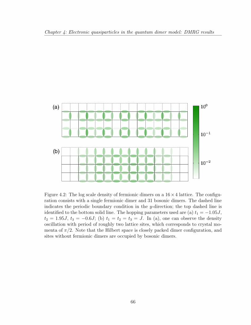
Chapter 4: Electronic quasiparticles in the quantum dimer model: DMRG results
Figure 4.2: The log scale density of fermionic dimers on a 16⇥4 lattice. The configu-ration consists with a single fermionic dimer and 31 bosonic dimers. The dashed lineindicates the periodic boundary condition in the y-direction; the top dashed line isidentified to the bottom solid line. The hopping parameters used are (a) t1 = �1.05J ,t2 = 1.95J , t3 = �0.6J ; (b) t1 = t2 = t3 = J . In (a), one can observe the densityoscillation with period of roughly two lattice sites, which corresponds to crystal mo-menta of ⇡/2. Note that the Hilbert space is closely packed dimer configuration, andsites without fermionic dimers are occupied by bosonic dimers.
66

Chapter 4: Electronic quasiparticles in the quantum dimer model: DMRG results
increasing the x-direction of lattice size, up to 32 ⇥ 4 lattice and observed the same
behavior, in both cases with dispersion minima at kx = ⇡/2 (Fig. 4.2(a)) and kx = 0
(Fig. 4.2(b)). A more quantitative analysis for the 32⇥4 lattice by Fourier transform
will follow below, together with the higher density calculation.
Note that Fig. 4.2(a) seems to break the translation symmetry in y-direction.
However, this is just a spontaneous symmetry breaking between the two degenerate
ground states; one being Fig. 4.2(a) and the other being Fig. 4.2(a) translated by
one lattice site in the y-direction. One can check this by computing the ground state
multiple times and obtaining both states. The fact that Fig. 4.2(b) does not break
the symmetry is also in accordance with our claim. Since the state of Fig. 4.2(b) has
only one Fermi surface centered at ~k = (0, 0), there are no degeneracy in the ground
state.
We would like to study the Friedel oscillation more quantitatively and verify
whether this feature survives when we increase the number of fermionic dimers, n. We
keep the lattice size as 32⇥4 and increase n up to 8, which corresponds to 1/16 doping.
Since the ‘defects’ of the system are the open boundaries, the Friedel oscillation is in
the cylinder direction. From the density profile ⇢(x, y), we define ⇢x(x) =P
y ⇢(x, y)
and perform Fourier transformation. The result is shown in Fig. 4.3. Note that we
have normalized the data by 1/n, and the magnitude 1 peak at kx = 0 indicates the
total density is n. Other than the kx = 0 peak, we can observe that there is a peak
at kx = 7⇡/8 in Fig. 4.3(a), where the parameter set used is the same as Fig. 4.2(a).
This peak is due to the Friedel oscillation, and indicates that kx = 7⇡/16 at the Fermi
level. Punk et al. (2015) showed the energy minimum is at ~k = (q, q) for q slightly
less than ⇡/2, and this is in good agreement with our result. Our calculation cannot
resolve the value of ky, but based on experiments and previous works one can argue
the energy minimum should be either at the origin (~k = (0, 0)) or along the diagonal
(~k = (q, q)). Therefore, we can conclude the dispersion of the dimer model in our
cylinder will have a minimum at ~k = (7⇡/16, ⇡/2), and in the large system limit this
will converge to a diagonal point ~k = (q, q) with 7⇡/16 q ⇡/2.
For Fig. 4.3(b), which used the same parameter set as Fig. 4.2(b), there is no peak
67
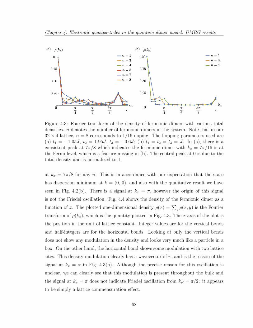
Chapter 4: Electronic quasiparticles in the quantum dimer model: DMRG results
Figure 4.3: Fourier transform of the density of fermionic dimers with various totaldensities. n denotes the number of fermionic dimers in the system. Note that in our32 ⇥ 4 lattice, n = 8 corresponds to 1/16 doping. The hopping parameters used are(a) t1 = �1.05J , t2 = 1.95J , t3 = �0.6J ; (b) t1 = t2 = t3 = J . In (a), there is aconsistent peak at 7⇡/8 which indicates the fermionic dimer with kx = 7⇡/16 is atthe Fermi level, which is a feature missing in (b). The central peak at 0 is due to thetotal density and is normalized to 1.
at kx = 7⇡/8 for any n. This is in accordance with our expectation that the state
has dispersion minimum at ~k = (0, 0), and also with the qualitative result we have
seen in Fig. 4.2(b). There is a signal at kx = ⇡, however the origin of this signal
is not the Friedel oscillation. Fig. 4.4 shows the density of the fermionic dimer as a
function of x. The plotted one-dimensional density ⇢(x) =P
y ⇢(x, y) is the Fourier
transform of ⇢(kx), which is the quantity plotted in Fig. 4.3. The x-axis of the plot is
the position in the unit of lattice constant. Integer values are for the vertical bonds
and half-integers are for the horizontal bonds. Looking at only the vertical bonds
does not show any modulation in the density and looks very much like a particle in a
box. On the other hand, the horizontal bond shows some modulation with two lattice
sites. This density modulation clearly has a wavevector of ⇡, and is the reason of the
signal at kx = ⇡ in Fig. 4.3(b). Although the precise reason for this oscillation is
unclear, we can clearly see that this modulation is present throughout the bulk and
the signal at kx = ⇡ does not indicate Friedel oscillation from kF = ⇡/2: it appears
to be simply a lattice commensuration e↵ect.
68

Chapter 4: Electronic quasiparticles in the quantum dimer model: DMRG results
Figure 4.4: One dimensional plot for fermionic dimer density (⇢(x) =P
y ⇢(x, y)) as afunction of distance in x direction, when n = 1. The x-axis unit is the lattice constant.Vertical bonds have integer x and colored yellow; horizontal bonds have half-integerx and colored blue. Notice the modulation is only present in the horizontal dimers.The system is a 32⇥ 4 cylinder with parameters t1 = t2 = t3 = J .
Note that we have not included the data obtained for n which mod (n, 4) = 2.
The calculations with such n had a stronger tendency towards wx 6= 0 topological
sector, and we had to decrease V further to keep the state in wx = 0 (For n = 2,
we needed V < 0.8). This seems to be an artifact of our system which is e↵ectively
one-dimensional and can only have four values of ky.
4.4 Entanglement entropy
We present the result for the computation of Renyi entropy to gain more infor-
mation about the ground state of the dimer model. First recall the definition of the
↵-th Renyi entanglement entropy:
S↵ =1
1� ↵ ln [Tr ⇢↵A] . (4.4)
Here, ⇢A is the reduced density matrix of partition A, i.e. ⇢A = TrB ⇢, where A[B is
the total system. Note that ↵-th Renyi entropy becomes the von Neumann entropy
in the ↵! 1 limit.
69
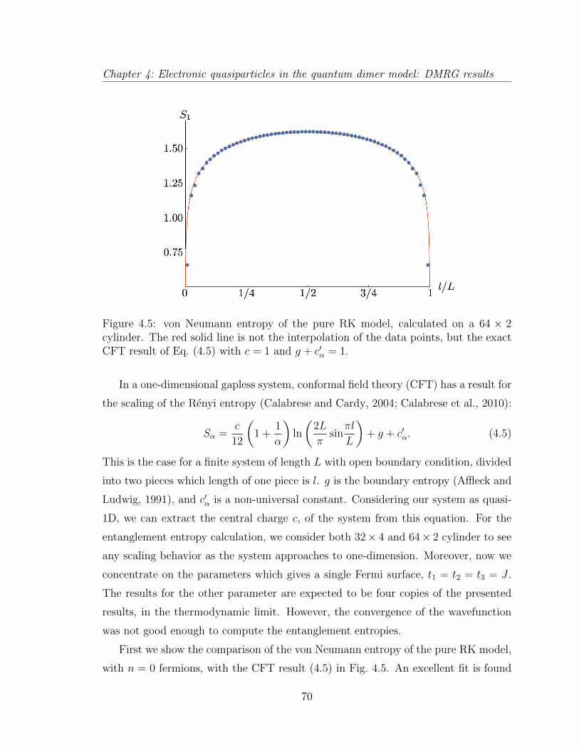
Chapter 4: Electronic quasiparticles in the quantum dimer model: DMRG results
Figure 4.5: von Neumann entropy of the pure RK model, calculated on a 64 ⇥ 2cylinder. The red solid line is not the interpolation of the data points, but the exactCFT result of Eq. (4.5) with c = 1 and g + c0↵ = 1.
In a one-dimensional gapless system, conformal field theory (CFT) has a result for
the scaling of the Renyi entropy (Calabrese and Cardy, 2004; Calabrese et al., 2010):
S↵ =c
12
✓1 +
1
↵
◆ln
✓2L
⇡sin
⇡l
L
◆+ g + c0↵. (4.5)
This is the case for a finite system of length L with open boundary condition, divided
into two pieces which length of one piece is l. g is the boundary entropy (A✏eck and
Ludwig, 1991), and c0↵ is a non-universal constant. Considering our system as quasi-
1D, we can extract the central charge c, of the system from this equation. For the
entanglement entropy calculation, we consider both 32⇥ 4 and 64⇥ 2 cylinder to see
any scaling behavior as the system approaches to one-dimension. Moreover, now we
concentrate on the parameters which gives a single Fermi surface, t1 = t2 = t3 = J .
The results for the other parameter are expected to be four copies of the presented
results, in the thermodynamic limit. However, the convergence of the wavefunction
was not good enough to compute the entanglement entropies.
First we show the comparison of the von Neumann entropy of the pure RK model,
with n = 0 fermions, with the CFT result (4.5) in Fig. 4.5. An excellent fit is found
70

Chapter 4: Electronic quasiparticles in the quantum dimer model: DMRG results
Figure 4.6: von Neumann entropy of the FL* phase with di↵erent fermionic dimerdensities. The system is a 64 ⇥ 2 cylinder with parameters t1 = t2 = t3 = J . L isthe length of the system, and l is the length of the subsystem. In the case of n = 0,which is a pure bosonic dimer model near the RK point, we get a nice fit to Eq. (4.5)with central charge 1.
for c = 1. The fermion-free dimer model is dual to a sine-Gordon model (Fradkin and
Kivelson, 1990; Read and Sachdev, 1990), and in 1+1 dimension this has a gapless
phase described by a massless relativistic boson with c = 1. The results of Fig. 4.5
are in accord with this expectation.
Turning to the case with fermions, the von Neumann entropy with dispersion
expected to have a single Fermi surface near ~k = (0, 0) is shown in Fig. 4.6. The
results are for 64⇥2 lattice. Data for 32⇥4 lattice are not shown, but are very similar
to the presented data (32⇥4 results are included in Fig. 4.7). We also include the data
from Fig. 4.5 for the case without any fermions. It is clear that these is an additional
contribution from the presence of the fermions, but it cannot be accounted for by
changing the central charge of the CFT. Fermions at non-zero density in an infinite
system should form a Fermi surface, and in the quasi-one dimensions geometry, each
Fermi point should yield an additional contribution of c = 1/2 of a chiral fermion. It
is clear that the data in Fig. 4.6 are not of this form.
Instead, we found that an excellent understanding of Fig. 4.6 is obtained by think-
ing about the limit of a very low density of fermions at the bottom of a quadratically
71
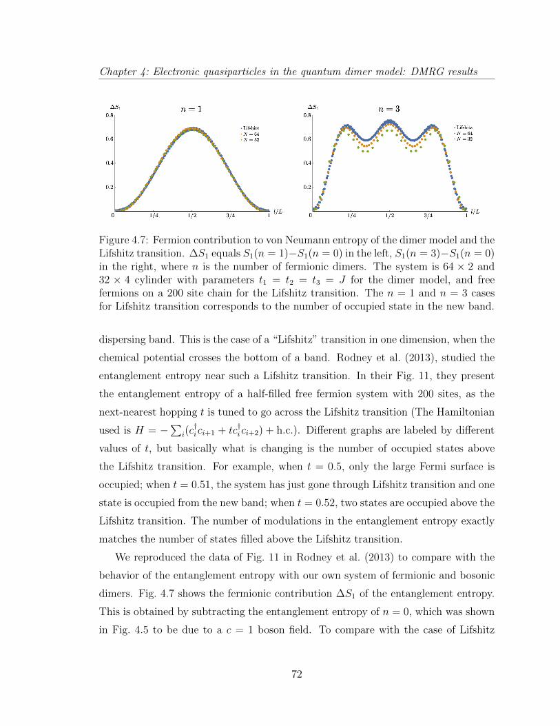
Chapter 4: Electronic quasiparticles in the quantum dimer model: DMRG results
Figure 4.7: Fermion contribution to von Neumann entropy of the dimer model and theLifshitz transition. �S1 equals S1(n = 1)�S1(n = 0) in the left, S1(n = 3)�S1(n = 0)in the right, where n is the number of fermionic dimers. The system is 64 ⇥ 2 and32 ⇥ 4 cylinder with parameters t1 = t2 = t3 = J for the dimer model, and freefermions on a 200 site chain for the Lifshitz transition. The n = 1 and n = 3 casesfor Lifshitz transition corresponds to the number of occupied state in the new band.
dispersing band. This is the case of a “Lifshitz” transition in one dimension, when the
chemical potential crosses the bottom of a band. Rodney et al. (2013), studied the
entanglement entropy near such a Lifshitz transition. In their Fig. 11, they present
the entanglement entropy of a half-filled free fermion system with 200 sites, as the
next-nearest hopping t is tuned to go across the Lifshitz transition (The Hamiltonian
used is H = �Pi(c†ici+1 + tc†ici+2) + h.c.). Di↵erent graphs are labeled by di↵erent
values of t, but basically what is changing is the number of occupied states above
the Lifshitz transition. For example, when t = 0.5, only the large Fermi surface is
occupied; when t = 0.51, the system has just gone through Lifshitz transition and one
state is occupied from the new band; when t = 0.52, two states are occupied above the
Lifshitz transition. The number of modulations in the entanglement entropy exactly
matches the number of states filled above the Lifshitz transition.
We reproduced the data of Fig. 11 in Rodney et al. (2013) to compare with the
behavior of the entanglement entropy with our own system of fermionic and bosonic
dimers. Fig. 4.7 shows the fermionic contribution �S1 of the entanglement entropy.
This is obtained by subtracting the entanglement entropy of n = 0, which was shown
in Fig. 4.5 to be due to a c = 1 boson field. To compare with the case of Lifshitz
72
Chapter 4: Electronic quasiparticles in the quantum dimer model: DMRG results
transition, we also subtract the entanglement entropy of the system with only one
large band occupied, which is t = 0.50 in the specific model, from the system with
one (three) state(s) occupied in the new band, corresponding to t = 0.51 (0.53); in
this case, the gapless fermions from the occupied large band contribute as a c = 1
field. As seen in Fig. 4.7, �S1 for n = 1 is nearly identical to the corresponding
entanglement entropy for the Lifshitz transition for free fermions with two di↵erent
lattice sizes. For n = 3, the value of �S1 decreases slightly as the length of the system
decreases, but the qualitative features remain the same. Note that in these data, only
the total length of the system was scaled to unity.
The above results provide strong evidence that the dimer model can be viewed as
two approximately independent systems: a background c = 1 boson corresponding
to the resonance between the dimers (both blue and green (Patel et al., 2016)), and
a dilute gas (of density p) of free fermions. These are precisely the characteristics
of the FL* state, which has an emergent gauge field (represented here by the c = 1
boson) and a Fermi surface of electron-like quasiparticles.
4.5 Outlook
The combination of our results on the density distribution and the entanglement
entropy confirm the expected appearance of a FL* state in the dimer model of Punk
et al. (2015). By general arguments (Senthil et al., 2004; Paramekanti and Vish-
wanath, 2004), the violation of the Luttinger theorem for a Fermi liquid requires that
the emergent gauge fields appear in the spectrum of the theory. Our results on the
entanglement entropy in a quasi-one-dimensional geometry are in accord with this
requirement, showing a background c = 1 boson that is expected from the gauge
theory of the dimer model (Fradkin and Kivelson, 1990; Read and Sachdev, 1990);
the boson represents the modes associated with the “resonance” between the dimers
around a plaquette. Above this gauge field background, we obtained evidence for a
gas of nearly-free fermions of density p, both in the density modulations and in the
entanglement entropy: in particular, the fermionic contribution to the entanglement
73
Chapter 4: Electronic quasiparticles in the quantum dimer model: DMRG results
entropy closely matched that of a dilute gas of free fermions near the bottom of a
quadratically dispersing band.
One possible direction to extend our work is to use the infinite-DMRG (iDMRG).
By using iDMRG we will be able to compute correlation functions of all length scales,
and can obtain momentum distribution and quasiparticle residue of Fermionic dimers.
Still, our momentum resolution in ky will be restricted by Ny.
Another approach is to use the recent proposal of DMRG in mixed real and
momentum space (Motruk et al., 2016). By this method we will be able to determine
ky more directly, which can be evidence of the existence of the hole pockets. Moreover,
Motruk et al. (2016) claims the computation time is reduced by more than an order
of magnitude, so this may allow us to include more sites in y-direction (in this case,
equivalently, more ky points).
74
Chapter 5
Quantum criticality of
reconstructing Fermi surfaces
5.1 Introduction
Quantum phase transitions between two Fermi liquids, one of which spontaneously
breaks translational symmetry and so reconstructs its Fermi surface, have been of
longstanding theoretical and experimental interest. Important new examples of ex-
perimental realizations have emerged in the past years, (Taillefer, 2010; Helm et al.,
2010; Nakai et al., 2010; Doiron-Leyraud and Taillefer, 2012) and so a full theo-
retical understanding is of some urgency. Next to immediate relevance for a class
of strongly correlated electron materials, the spin-fermion model has evolved into a
minimal model for itinerant lattice electrons with strong, commensurate magnetic
fluctuations that are believed to destroy the Fermi liquid behavior when tuned to the
critical point. How the compressible electron liquid, without Lorentz symmetry and
without particle-hole symmetry, behaves when its correlations become singular, could
provide some direction in the search for new universality classes beyond, for example,
the better-known Gross-Neveu model of Dirac fermions which enjoys more symme-
tries. However, despite several decades of theoretical work, key questions remain open
especially in the important case of two spatial dimensions.
75

Chapter 5: Quantum criticality of reconstructing Fermi surfaces
Early theories (Overhauser, 1962; Hertz, 1976; Millis, 1993; Sachdev et al., 1995;
Abanov et al., 2003; Moriya, 2012) for such quantum phase transitions focused on
e↵ective models for the quantum fluctuations of the order parameter, while treating
the Fermi surface reconstruction as an ancillary phenomenon. However, it has since
become clear (Abanov and Chubukov, 2000, 2004) that such an approach is inad-
equate, and the Fermi surface excitations are primary actors in the critical theory.
Metlitski and Sachdev (2010b) postulated a critical theory for Fermi surface recon-
struction, in which the Fermi surface excitations and the bosonic order parameter
were equally important and both acquired anomalous dimensions. These excitations
were strongly coupled to each other by a “Yukawa” coupling of universal strength,
and their correlators scaled with a common dynamic critical exponent, z. Explicit
computations were performed in the context of a 1/N expansion, where the physical
number of fermion flavors is generalized to N . Taking N large, one can formally reor-
ganize Wick’s theorem in powers of 1/N and then extrapolate results to the physical
number of fermion flavors. For the hot-spot field theory at the onset of spin-density
wave order, no such critical theory appeared at the two-loop level. Indeed, it was
pointed out that at higher loops (Lee, 2009; Metlitski and Sachdev, 2010a,b) there is
a breakdown of the 1/N expansion, and so it remained unclear whether the postulated
fixed point existed.
Here we address the problem of Fermi surface reconstruction at the onset of spin-
density wave order by an analysis based on a formally exact functional renormalization
group (fRG) approach. (Berges et al., 2002; Metzner et al., 2012) This RG approach
allows a computation of correlation function as a function of a continuous cuto↵ scale
⇤; from the “UV” at energies of the order of the bandwidth down to “infrared”
excitations at and in the vicinity of the Fermi surface. Nonuniversal quantities and
crossover scales can be extracted from the same solution which also yields the critical
exponents in the limit ⇤! 0. Combined with the potential to resolve the momentum
(and frequency) dependence or correlators along the Fermi surface, the fRG o↵ers
much more than the field theoretic RG or conventional ✏ expansion which is typically
used to extract the leading singularities only.
76
Chapter 5: Quantum criticality of reconstructing Fermi surfaces
In this chapter, we solve a set of coupled flow equations which treats the electrons
on equal footing to the collective, order-parameter fluctuations. We truncate the flow
equations to a set of discrete points on the Fermi surface. When projecting our cor-
relators onto the hot spot as a function of momenta, we establish the existence of a
fixed point with the scaling structure postulated in Metlitski and Sachdev (2010b),
describing the quantum phase transition between two Fermi liquids: from the metal
with preserved SU(2) spin symmetry to the metallic antiferromagnet which sponta-
neously breaks spin symmetry. A significant feature of our truncation is that it ties
the parameters controlling the order parameter fluctuations to those associated with
the fermion excitations, and this is important for a proper description of the scaling
structure. We present numerical estimates for the critical exponents of the boson and
fermion spectral functions, and for the variation in the fermionic quasiparticle residue
around the Fermi surface. During our computations, we keep the shape of the Fermi
surface fixed. In principle, one would have to allow for a flowing Fermi surface and
consequently a flowing hot spot. In such a truncation, the singular manifold becomes
a “moving target” and this significantly complicates the analysis.
The rest of our results are presented in Chapter 5.5. In Chapter 5.2, we introduce
the recently developed two-band spin-fermion model that has the additional appeal-
ing feature that it does not su↵er from the sign problem in quantum Monte Carlo
simulations. (Berg et al., 2012) In Chapter 5.3, we present the functional RG setup,
the truncation, and the cuto↵ functions. In Chapter 5.6, we conclude and suggest
interesting future directions resulting from this chapter.
5.2 Model
Our computation will be carried in the context of the “spin-fermion” model of
antiferromagnetic fluctuations in a Fermi liquid. (Abanov et al., 2003) This involves
a spin-density wave order parameter ~� at wave vector K = (⇡, ⇡) coupled to fermions
moving on a square lattice. The analytic analyses have focused on the vicinity of
the “hot spots” on the Fermi surface: These are the eight points on the Fermi surface
77
Chapter 5: Quantum criticality of reconstructing Fermi surfaces
which can generically be connected to each other by K. The fermion dispersions were
linearized and truncated around the hot spots. However a complete analysis requires
that we avoid the spurious singularities associated with truncated Fermi surfaces and
deal only with continuous Fermi surfaces. Here, we choose the Fermi surface config-
urations of a recent analysis (Berg et al., 2012) which allowed Monte Carlo studies
without a sign problem. The present work may be seen as complementary to Berg
et al. (2012): Here we especially focus on the universality class and critical properties.
This paves the way for an eventual comparison of our renormalization group results
with Monte Carlo. Our present method applies also to general Fermi surfaces and
provides access to real-time spectral functions which are not easily obtainable from
imaginary-time Monte Carlo.
The model of Berg et al. (2012) contains fermions in two bands, or two flavors, ↵,
↵ = 1, 2 (although our present method can also be applied to single band models),
coupled to ~� in the e↵ective action
�⇤UV
h , , ~�
i=
Z
k
X
↵=1,2
↵(k)
�ik0 + ⇠k,↵ 0
0 �ik0 + ⇠k,↵
! ↵(k)
+
Z
q
1
2~�(�q) �q2 + r
�~�(q) (5.1)
+
Z
k,q
� ~�(q)� 1(k + q)~� 2(k) + 2(k + q)~� 1(k)
�,
whereRkrepresents integrals over spatial momenta k = (kx, ky) over the Brillouin
zone, and frequencies k0. The fermion spinors are defined by ↵(k) =� ↵,"(k) ↵,#(k)
�,
↵ = 1, 2. We already introduce here the cuto↵ ⇤ along which we later integrate our
renormalization group flow toward ⇤ ! 0. With ⇤ = ⇤UV we have the bare lattice
action. The boson quadratic term consists of the control parameter r and a spatial
gradient squared to account for spatial variations of the order parameter field ~�. The
quantum dynamics of ~� will be generated in the RG flow; putting a q20 term into
Eq. (5.1) does not change our results. The fermion dispersions for nearest-neighbor
hopping are
⇠k,↵ = �2t↵,xcoskx � 2t↵,ycosky � µ↵. (5.2)
78
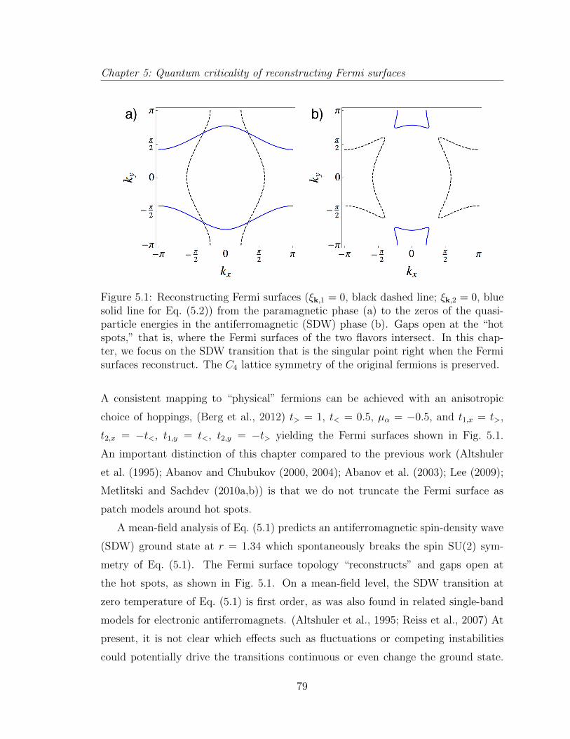
Chapter 5: Quantum criticality of reconstructing Fermi surfaces
Figure 5.1: Reconstructing Fermi surfaces (⇠k,1 = 0, black dashed line; ⇠k,2 = 0, bluesolid line for Eq. (5.2)) from the paramagnetic phase (a) to the zeros of the quasi-particle energies in the antiferromagnetic (SDW) phase (b). Gaps open at the “hotspots,” that is, where the Fermi surfaces of the two flavors intersect. In this chap-ter, we focus on the SDW transition that is the singular point right when the Fermisurfaces reconstruct. The C4 lattice symmetry of the original fermions is preserved.
A consistent mapping to “physical” fermions can be achieved with an anisotropic
choice of hoppings, (Berg et al., 2012) t> = 1, t< = 0.5, µ↵ = �0.5, and t1,x = t>,
t2,x = �t<, t1,y = t<, t2,y = �t> yielding the Fermi surfaces shown in Fig. 5.1.
An important distinction of this chapter compared to the previous work (Altshuler
et al. (1995); Abanov and Chubukov (2000, 2004); Abanov et al. (2003); Lee (2009);
Metlitski and Sachdev (2010a,b)) is that we do not truncate the Fermi surface as
patch models around hot spots.
A mean-field analysis of Eq. (5.1) predicts an antiferromagnetic spin-density wave
(SDW) ground state at r = 1.34 which spontaneously breaks the spin SU(2) sym-
metry of Eq. (5.1). The Fermi surface topology “reconstructs” and gaps open at
the hot spots, as shown in Fig. 5.1. On a mean-field level, the SDW transition at
zero temperature of Eq. (5.1) is first order, as was also found in related single-band
models for electronic antiferromagnets. (Altshuler et al., 1995; Reiss et al., 2007) At
present, it is not clear which e↵ects such as fluctuations or competing instabilities
could potentially drive the transitions continuous or even change the ground state.
79

Chapter 5: Quantum criticality of reconstructing Fermi surfaces
The same is true for the formation of SDWs with periods incommensurate with the
underlying lattice. In the present chapter, we ignore these complications and focus
our attention on continuous SDW transitions at zero temperature.
5.3 Functional Renormalization Group
Our RG analysis is based on the (formally exact) flow equation for the e↵ective
action �⇤R
h , , ~�
i, the generating functional for one-particle irreducible correlation
functions in the form derived by Wetterich. (Berges et al., 2002; Metzner et al.,
2012) The regulator R introduces a cuto↵ dependence into the e↵ective action so
that �⇤R smoothly interpolates between the bare action, Eq. (5.1), at the ultraviolet
scale �⇤=⇤UVR
h , , ~�
i= �⇤UV
h , , ~�
iand the fully renormalized e↵ective action
in the limit of vanishing cuto↵: lim⇤!0 �⇤R
h , , ~�
i= �
h , , ~�
i. The Wetterich
equation has a one-loop structure and in a vertex expansion the � functions for the
n-point correlators are determined by (cuto↵ derivatives of) one-particle irreducible
one-loop diagrams with fully dressed propagators and vertices. Upon self-consistent
integration of the coupled set of � functions, contributions of arbitrary high loop order
are generated. As we explain below, we truncate the e↵ective action to the full fermion
two-point function (including a fermion self-energy ⌃⇤f (k0,k)), the full bosonic two-
point function (including a bosonic self-energy ⌃⇤b (q0,q)), and the Yukawa coupling
�⇤.
Our results are obtained from the renormalization group flow of the action Eq. (5.1)
at the quantum-critical point (r = 0) under the formally exact evolution equation
(Metzner et al., 2012)
d
d⇤�⇤R [�, �] =
1
2Str
⇢R⇤
h�(2)⇤R [�, �] +R⇤
i�1�
. (5.3)
�(2)⇤R is the second derivative with respect to the fields defined below. R⇤ is a matrix
containing ⇤-dependent cuto↵ functions that regularizes the infrared singularities
of the fermion and boson propagators. The dot is shorthand notation for a scale
derivative R⇤ = @⇤R⇤. Both sides of this equation are projected onto a “super”-field
80
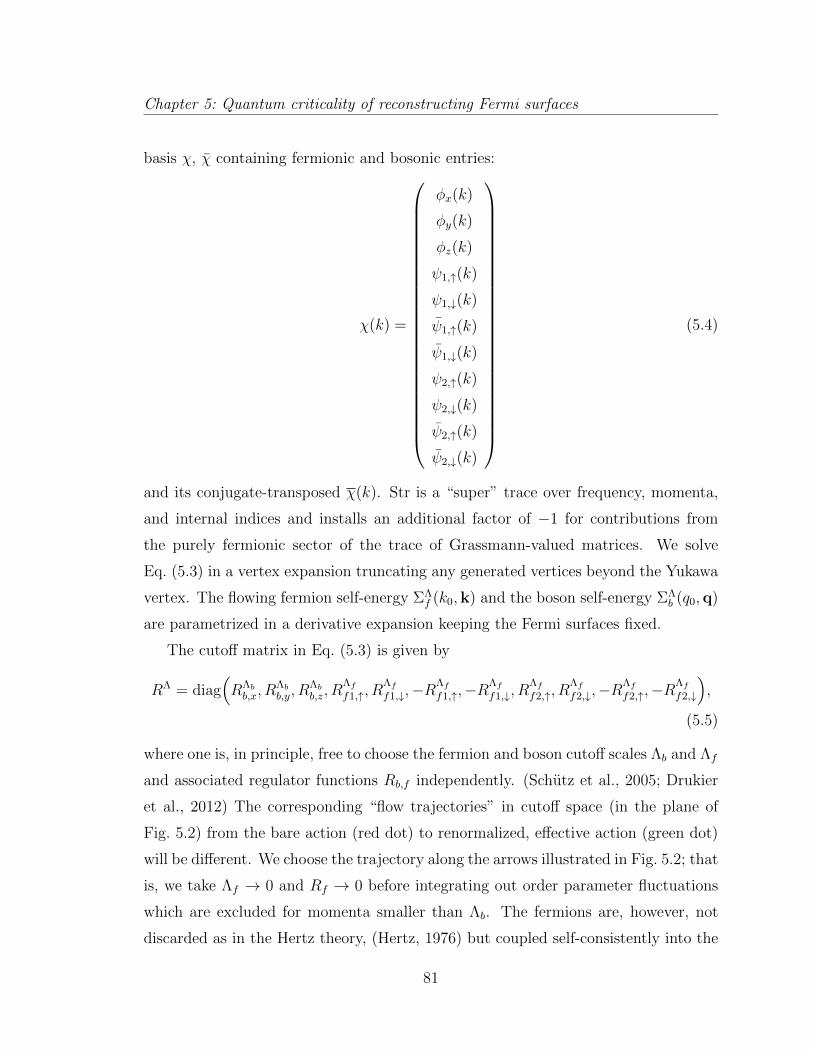
Chapter 5: Quantum criticality of reconstructing Fermi surfaces
basis �, � containing fermionic and bosonic entries:
�(k) =
0
BBBBBBBBBBBBBBBBBBBBBBBB@
�x(k)
�y(k)
�z(k)
1,"(k)
1,#(k)
1,"(k)
1,#(k)
2,"(k)
2,#(k)
2,"(k)
2,#(k)
1
CCCCCCCCCCCCCCCCCCCCCCCCA
(5.4)
and its conjugate-transposed �(k). Str is a “super” trace over frequency, momenta,
and internal indices and installs an additional factor of �1 for contributions from
the purely fermionic sector of the trace of Grassmann-valued matrices. We solve
Eq. (5.3) in a vertex expansion truncating any generated vertices beyond the Yukawa
vertex. The flowing fermion self-energy ⌃⇤f (k0,k) and the boson self-energy ⌃⇤
b (q0,q)
are parametrized in a derivative expansion keeping the Fermi surfaces fixed.
The cuto↵ matrix in Eq. (5.3) is given by
R⇤ = diag⇣R⇤
b
b,x, R⇤b
b,y, R⇤b
b,z, R⇤f
f1,", R⇤f
f1,#,�R⇤f
f1,",�R⇤f
f1,#, R⇤f
f2,", R⇤f
f2,#,�R⇤f
f2,",�R⇤f
f2,#⌘,
(5.5)
where one is, in principle, free to choose the fermion and boson cuto↵ scales ⇤b and ⇤f
and associated regulator functions Rb,f independently. (Schutz et al., 2005; Drukier
et al., 2012) The corresponding “flow trajectories” in cuto↵ space (in the plane of
Fig. 5.2) from the bare action (red dot) to renormalized, e↵ective action (green dot)
will be di↵erent. We choose the trajectory along the arrows illustrated in Fig. 5.2; that
is, we take ⇤f ! 0 and Rf ! 0 before integrating out order parameter fluctuations
which are excluded for momenta smaller than ⇤b. The fermions are, however, not
discarded as in the Hertz theory, (Hertz, 1976) but coupled self-consistently into the
81
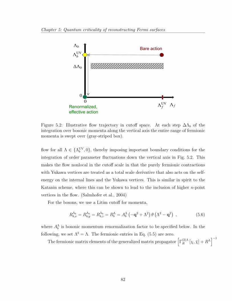
Chapter 5: Quantum criticality of reconstructing Fermi surfaces
Bare action
Renormalized, effective action
Figure 5.2: Illustrative flow trajectory in cuto↵ space. At each step �⇤b of theintegration over bosonic momenta along the vertical axis the entire range of fermionicmomenta is swept over (gray-striped box).
flow for all ⇤ 2 {⇤UVb , 0}, thereby imposing important boundary conditions for the
integration of order parameter fluctuations down the vertical axis in Fig. 5.2. This
makes the flow nonlocal in the cuto↵ scale in that the purely fermionic contractions
with Yukawa vertices are treated as a total scale derivative that also acts on the self-
energy on the internal lines and the Yukawa vertices. This is similar in spirit to the
Katanin scheme, where this can be shown to lead to the inclusion of higher n-point
vertices in the flow. (Salmhofer et al., 2004)
For the bosons, we use a Litim cuto↵ for momenta,
R⇤b
b,x = R⇤b
b,y = R⇤b
b,z = R⇤b = A⇤
b
��q2 + ⇤2�✓�⇤2 � q2
�, (5.6)
where A⇤b is bosonic momentum renormalization factor to be specified below. In the
following, we set ⇤b = ⇤. The fermionic entries in Eq. (5.5) are zero.
The fermionic matrix elements of the generalized matrix propagatorh�(2)⇤R [�, �] +R⇤
i�1
82

Chapter 5: Quantum criticality of reconstructing Fermi surfaces
occurring in Eq. (5.3) become
G⇤f1,�(k) = �h 1,�(k) 1,�(k)iR
= �" �!
�
��(k1)�⇤R[�,�]
��
��(k2)+R⇤
#�1
f1,��=�=0k1=k2=k
=�1
�ik0 + ⇠k,1 + ⌃⇤f1(k0,k)
, (5.7)
and analogously for the other flavor and spin components.
The explicitly cuto↵-dependent boson spin fluctuation propagators are
DR(q) ⌘ DRx (q) = �h�x(q)�x(�q)iR
= �" �!
�
��(q1)�⇤R[�,�]
��
��(q2)+R⇤
#�1
b,x�=�=0q1=q2=q
=�1
q2 + r + ⌃⇤b (q0,q) +R⇤
b
=
8<
:
�1q2+r+⌃⇤
b
(q0,q)|q| > ⇤
�1⇤2+r+⌃⇤
b
(q0,⇤)|q| < ⇤
, (5.8)
and analogously for the other spin projections y, z. The functional derivatives are
evaluated at zero fields here, as we approach the QCP from the paramagnetic phase.
The flow equation for the fermion self-energy (depicted diagrammatically in Fig. 5.3(a))
is
@⇤⌃⇤f1[k0,k] = 3
��⇤�2Z
q,R
G⇤f2(k + q)DR
b (q) , (5.9)
and similarly for flavor 2 upon interchanging 1 $ 2. We use a shorthand notation
encapsulating frequency, momentum integrations, and a cuto↵ derivative with respect
to the bosonic cuto↵ function:Rq,R
b
=R
dq02⇡
Rd2q(2⇡)2
h�R⇤
b @R⇤b
i.
The prefactors and signs of the flow equations are computed by comparing coe�-
cients between the left- and right-hand sides of Eq. (5.3) as outlined in Sec.II of Gies
and Wetterich (2002). The 11⇥11 Grassmann-valued (super-) matrices are evaluated
83

Chapter 5: Quantum criticality of reconstructing Fermi surfaces
Figure 5.3: Diagrammatic representation of the flow equation for the fermion self-energy ⌃⇤
f (k0,k) (a) and the Yukawa coupling (b). Straight lines denote Fermi prop-agators of flavors 1 and 2; wiggly line boson propagators are endowed with a regulatorR⇤. Intersections of wiggly with straight lines represent the Yukawa coupling. Thecuto↵ derivative with respect to R⇤ is implicit. All propagators and vertices are“dressed” self-consistently and are functions of ⇤.
using the GrassmannOps.m package in Mathematica. How to take a supertrace can
be found in Wegner (1998).
The boson self-energy is determined self-consistently from the particle-hole bubble
(Fig. 5.4) at all stages of the flow:
⌃⇤b (q0,q) = �
�⇧⇤(q0,q)� ⇧⇤(0,0)
�(5.10)
= 2��⇤�2Z
k
h �G⇤
f1(k + q)�G⇤f1(k)
�G⇤
f2(k)
+G⇤f1(k)
�G⇤
f2(k + q)�G⇤f2(k)
� i.
The following ansatz captures the leading frequency and momentum-dependence of
the particle-hole bubble:
⌃⇤b (q0,q) = Z⇤
b |q0| + (A⇤b � 1)q2 . (5.11)
At the yellow dot in Fig. 5.2, the Fermi propagators are still Fermi-liquid like (⌃⇤UVf↵ =
0) because we have not yet integrated out any order parameter fluctuations which,
by Fig. 5.3(a), generate a finite fermion self-energy. At that point, the coe�cients
Z⇤UVb , A⇤UV
b take finite numerical values. At all stages of the flow, when integrating
84

Chapter 5: Quantum criticality of reconstructing Fermi surfaces
Figure 5.4: Particle-hole bubbles used for the flow of the boson self-energy inEq. (5.11). All propagators and vertices are “dressed” self-consistently and dependon ⇤.
the flow down the vertical axis of Fig. 5.2, the bosonic Z and A factor are determined
self-consistently according to the prescription
Z⇤b = �⇧
⇤(q0,0)� ⇧⇤(0,0)
q0
���q0=⇤
,
A⇤b = 1� ⇧
⇤(0,q)� ⇧⇤(0,0)
q2
���qx
=⇤,qy
=0. (5.12)
This allows them to pick up potentially singular renormalizations during the flow.
The boson momentum factor is isotropic in momentum space; interchanging qx $ qy
delivers the same value for A⇤b .
The flow equation as per Fig. 5.3(b) for the Yukawa coupling is
@⇤�⇤ = � ��⇤�3
Z
q,R
G⇤f1(k + q)G⇤
f2(k + q)DRb (q)
���k0=0,k=kHS
. (5.13)
The explicit expressions of the flow equations and the numerical parameter used
are given in the next chapter.
85
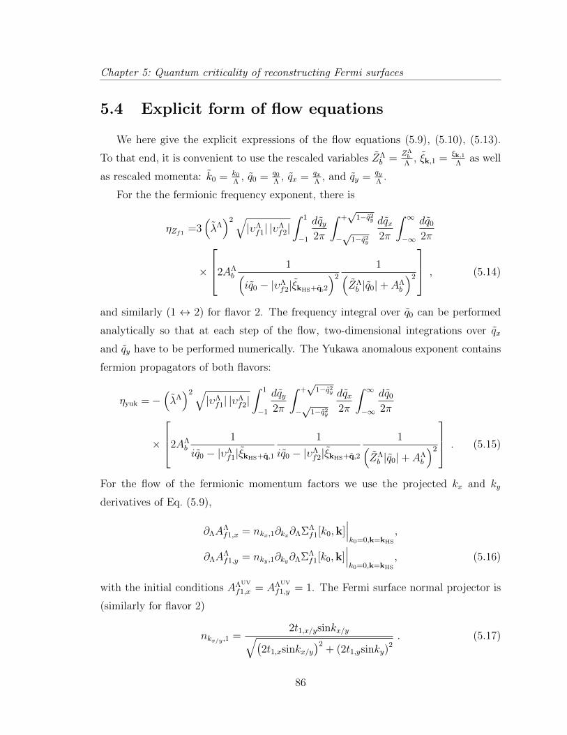
Chapter 5: Quantum criticality of reconstructing Fermi surfaces
5.4 Explicit form of flow equations
We here give the explicit expressions of the flow equations (5.9), (5.10), (5.13).
To that end, it is convenient to use the rescaled variables Z⇤b =
Z⇤b
⇤, ⇠k,1 =
⇠k,1⇤
as well
as rescaled momenta: k0 =k0⇤, q0 =
q0⇤, qx = q
x
⇤, and qy =
qy
⇤.
For the the fermionic frequency exponent, there is
⌘Zf1
=3⇣�⇤⌘2q
|�⇤f1| |�⇤f2|Z 1
�1
dqy2⇡
Z +p
1�q2y
�p
1�q2y
dqx2⇡
Z 1
�1
dq02⇡
⇥
2
642A⇤b
1⇣iq0 � |�⇤f2|⇠kHS+q,2
⌘2
1⇣Z⇤
b |q0| + A⇤b
⌘2
3
75 , (5.14)
and similarly (1 $ 2) for flavor 2. The frequency integral over q0 can be performed
analytically so that at each step of the flow, two-dimensional integrations over qx
and qy have to be performed numerically. The Yukawa anomalous exponent contains
fermion propagators of both flavors:
⌘yuk =�⇣�⇤⌘2q
|�⇤f1| |�⇤f2|Z 1
�1
dqy2⇡
Z +p
1�q2y
�p
1�q2y
dqx2⇡
Z 1
�1
dq02⇡
⇥
2
642A⇤b
1
iq0 � |�⇤f1|⇠kHS+q,1
1
iq0 � |�⇤f2|⇠kHS+q,2
1⇣Z⇤
b |q0| + A⇤b
⌘2
3
75 . (5.15)
For the flow of the fermionic momentum factors we use the projected kx and ky
derivatives of Eq. (5.9),
@⇤A⇤f1,x = nk
x
,1@kx
@⇤⌃⇤f1[k0,k]
���k0=0,k=kHS
,
@⇤A⇤f1,y = nk
y
,1@ky
@⇤⌃⇤f1[k0,k]
���k0=0,k=kHS
, (5.16)
with the initial conditions A⇤UV
f1,x = A⇤UV
f1,y = 1. The Fermi surface normal projector is
(similarly for flavor 2)
nkx/y
,1 =2t1,x/ysinkx/yq�
2t1,xsinkx/y�2
+ (2t1,ysinky)2. (5.17)
86
Chapter 5: Quantum criticality of reconstructing Fermi surfaces
The flow equations for the rescaled variables are A⇤f1,x =
A⇤f1,x
Z⇤f1
, A⇤f1,y =
A⇤f1,y
Z⇤f1
. With
⌘Zf1
given in Eq. (5.14), these take the form
⇤@⇤A⇤f1,x =
�⌘Z
f1� ⌘A
f1,x
�A⇤
f1,x,
⇤@⇤A⇤f1,y =
�⌘Z
f1� ⌘A
f1,y
�A⇤
f1,y , (5.18)
with the exponents ⌘Af1,x
= �d lnA⇤f1,x
d ln⇤, ⌘A
f1,y= �d lnA⇤
f1,y
d ln⇤.At every step of the flow,
we compute then per Eq. (5.25)
|�⇤f1| =
r⇣A⇤
f1,x
⌘2
+⇣A⇤
f1,y
⌘2
|r⇠1,k|k=kHS
. (5.19)
Expressions for the exponents:
⌘Af1,x
=� nkHS,x,1 3⇣�⇤⌘2q
|�⇤f1| |�⇤f2||�⇤f2|Af1,x
⇥Z 1
�1
dqy2⇡
Z +p
1�q2y
�p
1�q2y
dqx2⇡
Z 1
�1
dq02⇡
2A⇤b
2t2xsin (kHS,x + qx⇤)⇣iq0 � |�⇤f2|⇠kHS+q,2
⌘2
1⇣Z⇤
b |q0| + A⇤b
⌘2 ,
⌘Af1,y
=� nkHS,y,1 3⇣�⇤⌘2q
|�⇤f1| |�⇤f2||�⇤f1|Af1,y
⇥Z 1
�1
dqy2⇡
Z +p
1�q2y
�p
1�q2y
dqx2⇡
Z 1
�1
dq02⇡
2A⇤b
2t2ysin (kHS,y + qy⇤)⇣iq0 � |�⇤f2|⇠kHS+q,2
⌘2
1⇣Z⇤
b |q0| + A⇤b
⌘2 .
(5.20)
Finally, the (rescaled) boson frequency factor and momentum factor are self-
consistently determined from
Z⇤b =2
⇣�⇤⌘2q
|�⇤f1| |�⇤f2|Z ⇡
�⇡
dkx2⇡
Z ⇡
�⇡
dky2⇡
1
⇤2
⇥Z 1
�1
dk02⇡
" 1
i(k0 + 1)� |�⇤f1|⇠k,1� 1
ik0 � |�⇤f1|⇠k,1
!1
ik0 � |�⇤f2|⇠k,2+ (1$ 2)
#,
A⇤b =2
⇣�⇤⌘2q
|�⇤f1| |�⇤f2|Z ⇡
�⇡
dkx2⇡
Z ⇡
�⇡
dky2⇡
1
⇤2
⇥Z 1
�1
dk02⇡
" 1
ik0 � |�⇤f1|⇠k+qx
,1
� 1
ik0 � |�⇤f1|⇠k,1
!1
ik0 � |�⇤f2|⇠k,2+ (1$ 2)
#
qx
=⇤
.
(5.21)
87
Chapter 5: Quantum criticality of reconstructing Fermi surfaces
Equations (5.22), (5.14), (5.15), and (5.18)–(5.21) are solved numerically as a
function of flow parameter ⇤ = ⇤UVe�s so that s = 0 corresponds to the UV (⇤UV =
1). The hot spot coordinates are kHS,x = 1.0472, kHS,y = 2.0944. As initial conditions,
we choose �⇤UV = 0.25, Z⇤UVf1 = Z⇤UV
f2 = 1, and A⇤UVf1 = A⇤UV
f2 = 1. The initial values
for the boson propagator are Z⇤UVb = 0.052 and A⇤UV
b = 1.011.
5.5 Results
We now describe the key results obtained from a solution of the flow equations. (i)
We find an infrared strong-coupling fixed point for the Yukawa-coupling �⇤ which gov-
erns the RG flow of the coupled Fermi-Bose action down to the lowest scales ⇤! 0.
This induces scaling relations among the anomalous exponents for the Fermi velocity,
the quasiparticle weight, and the Yukawa vertex. (ii) Both the quasiparticle weight
and the Fermi velocity vanish as a power law when scaling the momenta toward the
hot spot; the Fermi velocity slower than the quasiparticle weight. (iii) The (quantum)
dynamical scaling of the electronic single-particle and collective spin fluctuations fol-
lows from an emergent dynamical exponent, attaining the same (fractional) value for
both fermions and bosons.
The centerpiece of our analysis is the flow equation for the Yukawa coupling:
⇤@⇤�⇤ =
✓1
4
�⌘Z
f1+ ⌘Z
f2+ ⌘A
f1+ ⌘A
f2
�� ⌘yuk � 1
2
◆�⇤ , (5.22)
where⇣�⇤⌘2
=��⇤�2
/(⇤q
Z⇤f1Z
⇤f2
qA⇤
f1A⇤f2) is rescaled by the frequency (Z⇤
f1) and
momentum (A⇤f1) derivatives of the fermion self-energy generated under the RG flow
as per Fig. 5.3(a). The power-law divergences as well as all other nonuniversal con-
tributions to the flow of the two fermion self-energy factors and the Yukawa coupling
itself are absorbed into the anomalous exponents:
⌘Zf1
= �d lnZ⇤f1
d ln⇤, ⌘A
f1= �d lnA⇤
f1
d ln⇤, ⌘yuk = �d ln�⇤
d ln⇤. (5.23)
⌘yuk is driven by the direct contribution to the flow of �⇤ exhibited in Fig. 5.3(b).
All couplings are projected to zero fermionic frequency, a discrete set of fermionic
88
Chapter 5: Quantum criticality of reconstructing Fermi surfaces
momenta on the Fermi surfaces, and zero bosonic frequency and momenta. This is
where the most singular renormalizations occur.
Specifically, the inverse quasi-particle weight is computed from the flowing self-
energy by (Honerkamp and Salmhofer, 2003)
Z⇤f1 = 1� @
@ik0⌃⇤
f1(k0,k)|k0=0,k=kF, (5.24)
where kF is a momentum on the Fermi surface and the initial condition is Z⇤UV
f1 = 1.
The momentum renormalization factor is obtained from a momentum gradient of the
fermion self-energy,
A⇤f1 = 1 +
|nk,1 ·r⌃⇤f1(k0,k)|
|r⇠k,1|���k0=0,k=kF
, (5.25)
with the initial condition A⇤UV
f1 = 1. Here, r =�@k
x
, @ky
�and nk,1 is unit normal
vector onto the Fermi surface of flavor 1. We see below that the momentum gradient
scales di↵erently than the frequency derivative at the quantum critical point. In a
di↵erent context, for Fermi systems with van Hove singularities, this asymmetry was
established to all orders in perturbation theory by Feldman and Salmhofer. (Feldman
and Salmhofer, 2008) Necessary conditions to discover this are (i) the codimension
of the Fermi surface manifold is greater than zero (it is zero in a one-dimensional
Fermi systems) and (ii) one includes the additional, relevant transversal momentum
direction parallel to the Fermi surface into the analysis.
With these definitions, the scale-dependent “dressed” fermion propagator which
occurs self-consistently in all RG equations becomes
G⇤f1(k) =
�1�ik0 + ⇠k,1 + ⌃⇤
f1(k0,k)=
Z⇤f1
ik0 � |�⇤f1|⇠k,1, (5.26)
with Z⇤f1 = 1/Z⇤
f1 resembling the quasiparticle weight at low energies and the e↵ective
modulus of the Fermi velocity |�⇤f1| =A⇤
f1
Z⇤f1.
A self-consistent numerical solution of the flow equations for the Yukawa vertex
�⇤, the fermion self-energy ⌃⇤f (k0,k), and the boson self-energy ⌃⇤
b (q0,q) is attracted
toward an infrared strong-coupling fixed point. As can be read o↵ from Fig. 5.5, the
89
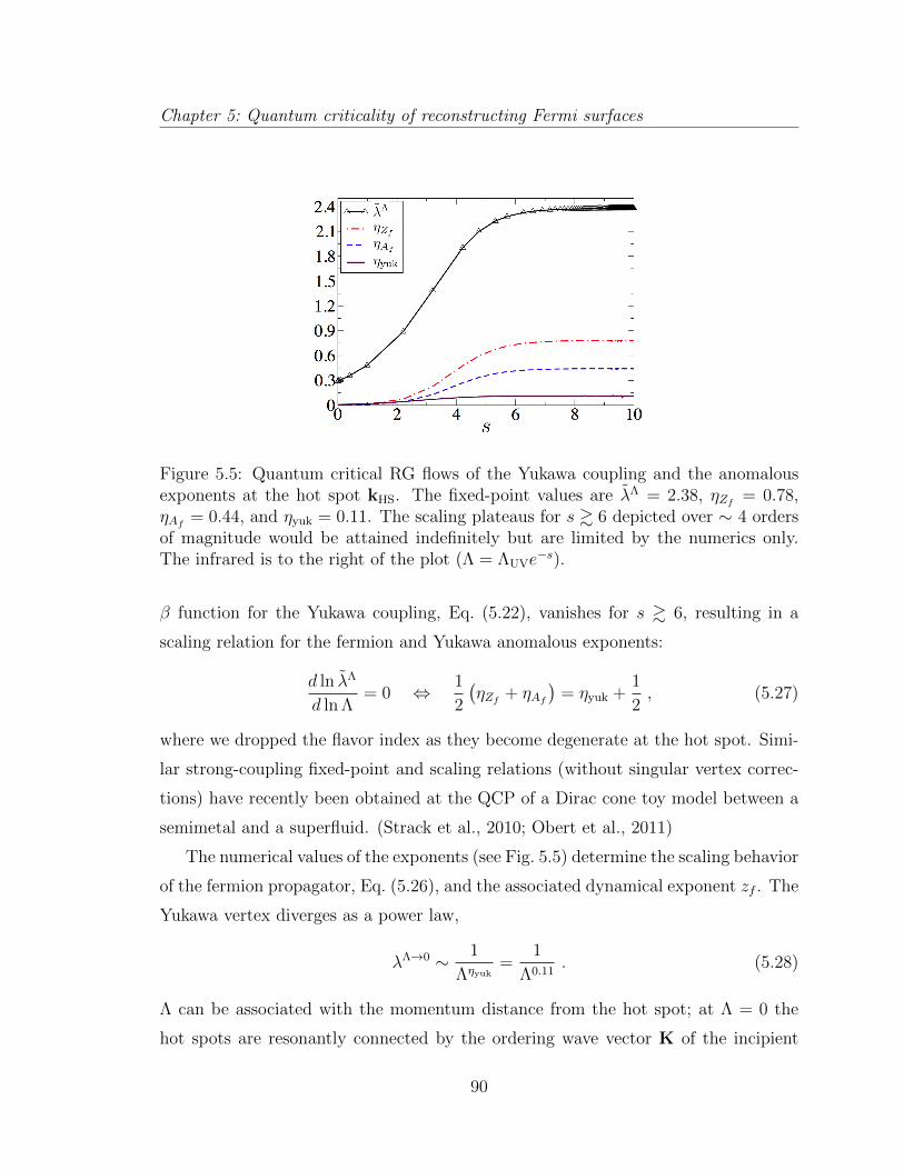
Chapter 5: Quantum criticality of reconstructing Fermi surfaces
Figure 5.5: Quantum critical RG flows of the Yukawa coupling and the anomalousexponents at the hot spot kHS. The fixed-point values are �⇤ = 2.38, ⌘Z
f
= 0.78,⌘A
f
= 0.44, and ⌘yuk = 0.11. The scaling plateaus for s & 6 depicted over ⇠ 4 ordersof magnitude would be attained indefinitely but are limited by the numerics only.The infrared is to the right of the plot (⇤ = ⇤UVe�s).
� function for the Yukawa coupling, Eq. (5.22), vanishes for s & 6, resulting in a
scaling relation for the fermion and Yukawa anomalous exponents:
d ln �⇤
d ln⇤= 0 , 1
2
�⌘Z
f
+ ⌘Af
�= ⌘yuk +
1
2, (5.27)
where we dropped the flavor index as they become degenerate at the hot spot. Simi-
lar strong-coupling fixed-point and scaling relations (without singular vertex correc-
tions) have recently been obtained at the QCP of a Dirac cone toy model between a
semimetal and a superfluid. (Strack et al., 2010; Obert et al., 2011)
The numerical values of the exponents (see Fig. 5.5) determine the scaling behavior
of the fermion propagator, Eq. (5.26), and the associated dynamical exponent zf . The
Yukawa vertex diverges as a power law,
�⇤!0 ⇠ 1
⇤⌘yuk=
1
⇤0.11. (5.28)
⇤ can be associated with the momentum distance from the hot spot; at ⇤ = 0 the
hot spots are resonantly connected by the ordering wave vector K of the incipient
90
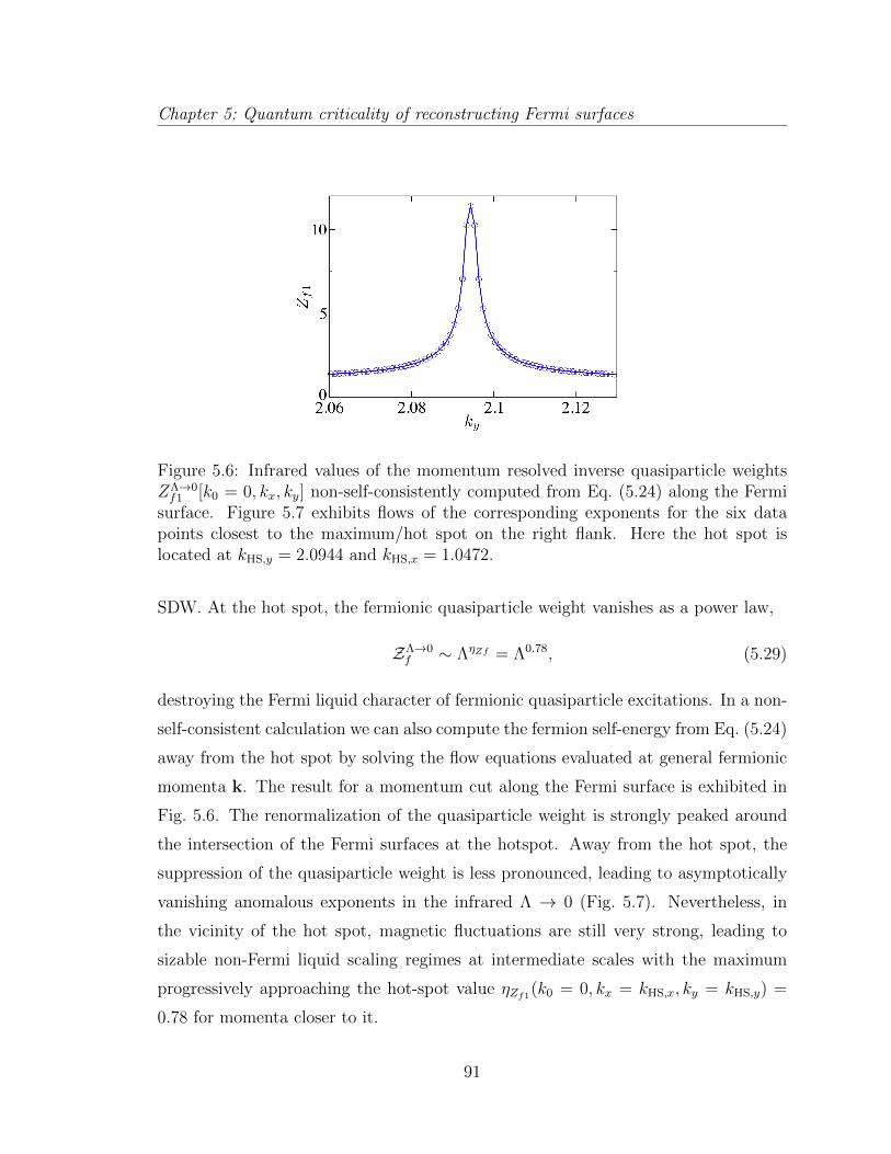
Chapter 5: Quantum criticality of reconstructing Fermi surfaces
Figure 5.6: Infrared values of the momentum resolved inverse quasiparticle weightsZ⇤!0
f1 [k0 = 0, kx, ky] non-self-consistently computed from Eq. (5.24) along the Fermisurface. Figure 5.7 exhibits flows of the corresponding exponents for the six datapoints closest to the maximum/hot spot on the right flank. Here the hot spot islocated at kHS,y = 2.0944 and kHS,x = 1.0472.
SDW. At the hot spot, the fermionic quasiparticle weight vanishes as a power law,
Z⇤!0f ⇠ ⇤⌘
Zf = ⇤0.78, (5.29)
destroying the Fermi liquid character of fermionic quasiparticle excitations. In a non-
self-consistent calculation we can also compute the fermion self-energy from Eq. (5.24)
away from the hot spot by solving the flow equations evaluated at general fermionic
momenta k. The result for a momentum cut along the Fermi surface is exhibited in
Fig. 5.6. The renormalization of the quasiparticle weight is strongly peaked around
the intersection of the Fermi surfaces at the hotspot. Away from the hot spot, the
suppression of the quasiparticle weight is less pronounced, leading to asymptotically
vanishing anomalous exponents in the infrared ⇤ ! 0 (Fig. 5.7). Nevertheless, in
the vicinity of the hot spot, magnetic fluctuations are still very strong, leading to
sizable non-Fermi liquid scaling regimes at intermediate scales with the maximum
progressively approaching the hot-spot value ⌘Zf1(k0 = 0, kx = kHS,x, ky = kHS,y) =
0.78 for momenta closer to it.
91
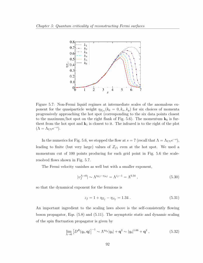
Chapter 5: Quantum criticality of reconstructing Fermi surfaces
Figure 5.7: Non-Fermi liquid regimes at intermediate scales of the anomalous ex-ponent for the quasiparticle weight ⌘Z
f1(k0 = 0, kx, ky) for six choices of momenta
progressively approaching the hot spot (corresponding to the six data points closestto the maximum/hot spot on the right flank of Fig. 5.6). The momentum k6 is fur-thest from the hot spot and k1 is closest to it. The infrared is to the right of the plot(⇤ = ⇤UVe�s).
In the numerics for Fig. 5.6, we stopped the flow at s = 7 (recall that ⇤ = ⇤UVe�s),
leading to finite (but very large) values of Zf1 even at the hot spot. We used a
momentum cut of 100 points producing for each grid point in Fig. 5.6 the scale-
resolved flows shown in Fig. 5.7.
The Fermi velocity vanishes as well but with a smaller exponent,
|�⇤!0f | ⇠ ⇤⌘
Zf
�⌘Af = ⇤z
f
�1 = ⇤0.34 , (5.30)
so that the dynamical exponent for the fermions is
zf = 1 + ⌘Zf
� ⌘Af
= 1.34 . (5.31)
An important ingredient to the scaling laws above is the self-consistently flowing
boson propagator, Eqs. (5.8) and (5.11). The asymptotic static and dynamic scaling
of the spin fluctuation propagator is given by
lim⇤!0
⇥DR(q0,q)
⇤�1 ⇠ ⇤⌘Z
b |q0| + q2 ⇠ |q0|1.66 + q2 , (5.32)
92
Chapter 5: Quantum criticality of reconstructing Fermi surfaces
with ⌘Zb
= 0.66. Remarkably, the boson dynamical exponent,
zb = 2� ⌘Zb
= 1.34 = zf , (5.33)
takes the same value as the fermion dynamical exponent. It is a distinguishing fea-
ture of this infrared fixed-point of electrons in metals at a SDW transition that the
dynamical exponent attains fractional value di↵erent from 1 (which is the exact value
for quantum-critical fermion systems with Lorentz-symmetry; see Janssen and Gies
(2012) and references therein) and di↵erent from 2 (which is the mean-field value of
the Hertz theory (Hertz, 1976)). Our fermion anomalous dimensions and z can be
mapped to those of Metlitski and Sachdev (2010b) for values of the Fermi velocity-
anisotropy in a range around ↵ ⇡ 0.5 and upon ignoring the marginal RG flow of ↵
(which is implicitly assumed in (5.25)); our boson anomalous dimension renormaliz-
ing the q2 term in the propagator is essentially zero, and we trace this to di↵erences
in the RG scheme from Metlitski and Sachdev (2010b).
5.6 Conclusion
This chapter was dedicated to the critical behavior of compressible, electronic
quantum matter in two-dimensional lattices interacting with self-generated, singular
antiferromagnetic fluctuations. We generalized previous hot-spot theories to full “UV-
completed” Fermi surfaces free of spurious edge singularities in a model that can
also be analyzed with quantum Monte Carlo. This should enable a cross-fertilizing
comparison of results obtained with di↵erent methods for this problem. We provided
first quantitative estimates for the critical exponents of the single-particle and spin
fluctuations correlators which deviate strongly from the Hertz-Millis values. The
solution of our RG equations was attracted toward a stable, strong-coupling fixed
point, resulting in a common dynamic exponent for the fermions and the bosons.
It would be interesting to classify all relevant operators to our fixed point and
investigate the stability of our strong-coupling fixed point further. As a first simple
step in this direction, we have extended the truncation for the fermion dispersions to
93

Chapter 5: Quantum criticality of reconstructing Fermi surfaces
allow for changes in the Fermi surface curvature (keeping the position of the hot spot
fixed). A scale-dependent ↵⇤ that modifies the hoppings, t1,x/y ! t1,x/y + ↵⇤ and
t2,x/y ! t2,x/y � ↵⇤, does the job. We found only relatively small, finite renormaliza-
tions of ↵⇤. However, a proper self-consistent investigation of a flowing Fermi surface
with the full dispersion used in this paper requires an advanced truncation and likely
also a self-consistent determination also of the position of the Fermi surfaces and
the hot spots as a function of ⇤. Potential tendencies toward magnetic ordering at
incommensurate wave vectors might also be captured that way. Such a state-of-the-
art truncation was recently presented for self-energy flows in the repulsive Hubbard
model close to van Hove filling. (Giering and Salmhofer, 2012)
Other promising future directions are the inclusion of (d-wave) superconductivity,
(Sedeki et al., 2012) an extension to the quantum-critical regime at finite tempera-
tures, and the exploration of the antiferromagnetic phase with broken symmetry close
to the quantum critical point. The latter can be achieved, for example, by generaliz-
ing Strack et al. (2008) from the superfluid O(2) case to the staggered O(3) case for
the spin-fermion model.
94
Bibliography
Abanin, D. A., Parameswaran, S. A., and Sondhi, S. L., 2009. Charge 2e Skyrmionsin Bilayer Graphene. Phys. Rev. Lett., 103:076802.
Abanov, A. and Chubukov, A., 2004. Anomalous Scaling at the Quantum CriticalPoint in Itinerant Antiferromagnets. Phys. Rev. Lett., 93:255702.
Abanov, A. and Chubukov, A. V., 2000. Spin-Fermion Model near the Quantum Crit-ical Point: One-Loop Renormalization Group Results. Phys. Rev. Lett., 84:5608.
Abanov, A., Chubukov, A. V., and Schmalian, J., 2003. Quantum-critical theoryof the spin-fermion model and its application to cuprates: Normal state analysis.Advances in Physics, 52(3):119.
Abanov, A. andWiegmann, P., 2000. Theta-terms in nonlinear sigma-models. NuclearPhysics B, 570(3):685 .
A✏eck, I. and Ludwig, A. W. W., 1991. Universal noninteger “ground-state degen-eracy” in critical quantum systems. Phys. Rev. Lett., 67:161.
Albuquerque, A. F., Schwandt, D., Hetenyi, B., et al., 2011. Phase diagram of a frus-trated quantum antiferromagnet on the honeycomb lattice: Magnetic order versusvalence-bond crystal formation. Phys. Rev. B, 84:024406.
Altshuler, B. L., Io↵e, L. B., and Millis, A. J., 1995. CriticalbehavioroftheT =0 2kFdensity-wave phase transition in a two-dimensional Fermi liquid. Phys. Rev. B,52:5563.
Berg, E., Metlitski, M. A., and Sachdev, S., 2012. Sign-Problem–Free Quantum MonteCarlo of the Onset of Antiferromagnetism in Metals. Science, 338(6114):1606.
Berges, J., Tetradis, N., and Wetterich, C., 2002. Non-perturbative renormalizationflow in quantum field theory and statistical physics. Physics Reports, 363(46):223 .Renormalization group theory in the new millennium. {IV}.
Block, M. S., Melko, R. G., and Kaul, R. K., 2013. Fate of CPN�1 Fixed Points withq Monopoles. Phys. Rev. Lett., 111:137202.
95
Bibliography
Bolotin, K. I., Ghahari, F., Shulman, M. D., et al., 2009. Observation of the fractionalquantum Hall e↵ect in graphene. Nature, 462(7270):196.
Calabrese, P., Campostrini, M., Essler, F., and Nienhuis, B., 2010. Parity E↵ectsin the Scaling of Block Entanglement in Gapless Spin Chains. Phys. Rev. Lett.,104:095701.
Calabrese, P. and Cardy, J., 2004. Entanglement entropy and quantum field theory.Journal of Statistical Mechanics: Theory and Experiment, 2004(06):P06002.
Castro Neto, A. H., Guinea, F., Peres, N. M. R., et al., 2009. The electronic propertiesof graphene. Rev. Mod. Phys., 81:109.
Checkelsky, J. G., Li, L., and Ong, N. P., 2009. Divergent resistance at the Diracpoint in graphene: Evidence for a transition in a high magnetic field. Phys. Rev.B, 79:115434.
Chubukov, A. V. and Morr, D. K., 1995. Phase transition, longitudinal spin fluctua-tions, and scaling in a two-layer antiferromagnet. Phys. Rev. B, 52:3521.
Chubukov, A. V., Sachdev, S., and Ye, J., 1994. Theory of two-dimensional quantumHeisenberg antiferromagnets with a nearly critical ground state. Phys. Rev. B,49:11919.
Clark, B. K., Abanin, D. A., and Sondhi, S. L., 2011. Nature of the Spin Liquid Stateof the Hubbard Model on a Honeycomb Lattice. Phys. Rev. Lett., 107:087204.
Cohen-Tannoudji, C., Grynberg, G., and Dupont-Roc, J., 1992. Atom-Photon Inter-actions: Basic Processes and Applications (Wiley, New York).
Cvetkovic, V., Throckmorton, R. E., and Vafek, O., 2012. Electronic multicriticalityin bilayer graphene. Phys. Rev. B, 86:075467.
Dhochak, K., Shimshoni, E., and Berg, E., 2015. Spontaneous layer polarization andconducting domain walls in the quantum Hall regime of bilayer graphene. Phys.Rev. B, 91:165107.
Doiron-Leyraud, N. and Taillefer, L., 2012. Quantum critical point for stripe order:An organizing principle of cuprate superconductivity. Physica C: Superconductivity,481:161 .
Drukier, C., Bartosch, L., Isidori, A., and Kopietz, P., 2012. Functional renormaliza-tion group approach to the Ising-nematic quantum critical point of two-dimensionalmetals. Phys. Rev. B, 85:245120.
96
Bibliography
Eisenstein, J., 2014. Exciton Condensation in Bilayer Quantum Hall Systems. AnnualReview of Condensed Matter Physics, 5(1):159.
Eisert, J., Cramer, M., and Plenio, M. B., 2010. Colloquium : Area laws for theentanglement entropy. Rev. Mod. Phys., 82:277.
Feldman, B. E., Krauss, B., Smet, J. H., and Yacoby, A., 2012. UnconventionalSequence of Fractional Quantum Hall States in Suspended Graphene. Science,337(6099):1196.
Feldman, J. and Salmhofer, M., 2008. Singular Fermi Surfaces II: The Two-Dimensional Case. Reviews in Mathematical Physics, 20(03):275.
Fradkin, E. and Kivelson, S. A., 1990. Short range resonating valence bond theoriesand superconductivity. Mod. Phys. Lett. B, 04(03):225.
Freitag, F., Trbovic, J., Weiss, M., and Schonenberger, C., 2012. SpontaneouslyGapped Ground State in Suspended Bilayer Graphene. Phys. Rev. Lett., 108:076602.
Freitag, F., Weiss, M., Maurand, R., et al., 2013. Spin symmetry of the bilayergraphene ground state. Phys. Rev. B, 87:161402.
Fu, L., Sachdev, S., and Xu, C., 2011. Geometric phases and competing orders in twodimensions. Phys. Rev. B, 83:165123.
Ganesh, R., van den Brink, J., and Nishimoto, S., 2013. Deconfined Criticality in theFrustrated Heisenberg Honeycomb Antiferromagnet. Phys. Rev. Lett., 110:127203.
Geim, A. K. and Grigorieva, I. V., 2013. Van der Waals heterostructures. Nature,499(7459):419.
Geim, A. K. and Novoselov, K. S., 2007. The rise of graphene. Nature Materials,6(3):183.
Giamarchi, T., 2004. Quantum physics in one dimension (Clarendon Press).
Giering, K.-U. and Salmhofer, M., 2012. Self-energy flows in the two-dimensionalrepulsive Hubbard model. Phys. Rev. B, 86:245122.
Gies, H. and Wetterich, C., 2002. Renormalization flow of bound states. Phys. Rev.D, 65:065001.
Gong, S.-S., Sheng, D. N., Motrunich, O. I., and Fisher, M. P. A., 2013. Phasediagram of the spin-1
2J1-J2 Heisenberg model on a honeycomb lattice. Phys. Rev.
B, 88:165138.
97
Bibliography
Grover, T. and Senthil, T., 2007. Quantum Spin Nematics, Dimerization, and De-confined Criticality in Quasi-1D Spin-One Magnets. Phys. Rev. Lett., 98:247202.
Grover, T. and Senthil, T., 2008. Topological Spin Hall States, Charged Skyrmions,and Superconductivity in Two Dimensions. Phys. Rev. Lett., 100:156804.
Halboth, C. J. and Metzner, W., 2000. Renormalization-group analysis of the two-dimensional Hubbard model. Phys. Rev. B, 61:7364.
Helm, T., Kartsovnik, M. V., Sheikin, I., et al., 2010. Magnetic Breakdown in theElectron-Doped Cuprate Superconductor Nd2�xCexCuO4: The Reconstructed FermiSurface Survives in the Strongly Overdoped Regime. Phys. Rev. Lett., 105:247002.
Herbut, I. F., 2007. SO(3) symmetry between Neel and ferromagnetic order parame-ters for graphene in a magnetic field. Phys. Rev. B, 76:085432.
Herbut, I. F., Lu, C.-K., and Roy, B., 2012. Conserved charges of order-parametertextures in Dirac systems. Phys. Rev. B, 86:075101.
Hertz, J. A., 1976. Quantum critical phenomena. Phys. Rev. B, 14:1165.
Hida, K., 1990. Low Temperature Properties of the Double Layer Quantum HeisenbergAntiferromagnet -Modified Spin Wave Method-. Journal of the Physical Society ofJapan, 59(6):2230.
Honerkamp, C. and Salmhofer, M., 2001. Temperature-flow renormalization groupand the competition between superconductivity and ferromagnetism. Phys. Rev. B,64:184516.
Honerkamp, C. and Salmhofer, M., 2003. Flow of the quasiparticle weight in the N-patch renormalization group scheme. Phys. Rev. B, 67:174504.
Hou, C.-Y., Chamon, C., and Mudry, C., 2007. Electron Fractionalization in Two-Dimensional Graphenelike Structures. Phys. Rev. Lett., 98:186809.
Hou, C.-Y., Chamon, C., and Mudry, C., 2010. Deconfined fractional electric chargesin graphene at high magnetic fields. Phys. Rev. B, 81:075427.
Jackiw, R. and Rossi, P., 1981. Zero modes of the vortex-fermion system. NuclearPhysics B, 190(4):681 .
Janssen, L. and Gies, H., 2012. Critical behavior of the (2 + 1)-dimensional Thirringmodel. Phys. Rev. D, 86:105007.
Jiang, H.-C., Wang, Z., and Balents, L., 2012. Identifying topological order by entan-glement entropy. Nature Physics, 8(12):902.
98
Bibliography
Jung, J. and MacDonald, A. H., 2009. Theory of the magnetic-field-induced insulatorin neutral graphene sheets. Phys. Rev. B, 80:235417.
Kharitonov, M., 2012a. Phase diagram for the ⌫ = 0 quantum Hall state in monolayergraphene. Phys. Rev. B, 85:155439.
Kharitonov, M., 2012b. Canted Antiferromagnetic Phase of the ⌫=0 Quantum HallState in Bilayer Graphene. Phys. Rev. Lett., 109:046803.
Kharitonov, M., 2012c. Edge excitations of the canted antiferromagnetic phase ofthe ⌫ = 0 quantum Hall state in graphene: A simplified analysis. Phys. Rev. B,86:075450.
Kharitonov, M., 2012d. Antiferromagnetic state in bilayer graphene. Phys. Rev. B,86:195435.
Kopietz, P., Bartosch, L., and Schutz, F., 2010. Introduction to the functional renor-malization group, volume 798 (Springer).
Kotov, V. N., Uchoa, B., Pereira, V. M., et al., 2012. Electron-Electron Interactionsin Graphene: Current Status and Perspectives. Rev. Mod. Phys., 84:1067.
Laflorencie, N., Sørensen, E. S., Chang, M.-S., and A✏eck, I., 2006. Boundary E↵ectsin the Critical Scaling of Entanglement Entropy in 1D Systems. Phys. Rev. Lett.,96:100603.
Landau, L. D., Lifshitz, E. M., and Pitaevskii, L. P., 1980. Statistical Physics(Butterworth-Heinemann).
Lang, T. C., Meng, Z. Y., Muramatsu, A., et al., 2013. Dimerized Solids and Res-onating Plaquette Order in SU(N)-Dirac Fermions. Phys. Rev. Lett., 111:066401.
Lang, T. C., Meng, Z. Y., Scherer, M. M., et al., 2012. Antiferromagnetism inthe Hubbard Model on the Bernal-Stacked Honeycomb Bilayer. Phys. Rev. Lett.,109:126402.
Lee, D.-H. and Kane, C. L., 1990. Boson-vortex-Skyrmion duality, spin-singlet frac-tional quantum Hall e↵ect, and spin-1/2 anyon superconductivity. Phys. Rev. Lett.,64:1313.
Lee, J. and Sachdev, S., 2014. Deconfined criticality in bilayer graphene. Phys. Rev.B, 90:195427.
Lee, P. A. and Nagaosa, N., 1992. Gauge theory of the normal state of high-Tc
superconductors. Phys. Rev. B, 46:5621.
99
Bibliography
Lee, S.-S., 2009. Low-energy e↵ective theory of Fermi surface coupled with U(1) gaugefield in 2 + 1 dimensions. Phys. Rev. B, 80:165102.
Levin, M. and Senthil, T., 2004. Deconfined quantum criticality and Neel order viadimer disorder. Phys. Rev. B, 70:220403.
Lu, C.-K. and Herbut, I. F., 2012. Zero Modes and Charged Skyrmions in GrapheneBilayer. Phys. Rev. Lett., 108:266402.
MacDonald, A. H., Girvin, S. M., and Yoshioka, D., 1988. tU
expansion for theHubbard model. Phys. Rev. B, 37:9753.
Maher, P., Dean, C. R., Young, A. F., et al., 2013. Evidence for a spin phase transitionat charge neutrality in bilayer graphene. Nature Physics, 9(3):154.
McCann, E. and Fal’ko, V. I., 2006. Landau-Level Degeneracy and Quantum HallE↵ect in a Graphite Bilayer. Phys. Rev. Lett., 96:086805.
Metlitski, M. A. and Sachdev, S., 2010a. Quantum phase transitions of metals in twospatial dimensions. I. Ising-nematic order. Phys. Rev. B, 82:075127.
Metlitski, M. A. and Sachdev, S., 2010b. Quantum phase transitions of metals in twospatial dimensions. II. Spin density wave order. Phys. Rev. B, 82:075128.
Metzner, W., Salmhofer, M., Honerkamp, C., et al., 2012. Functional renormalizationgroup approach to correlated fermion systems. Rev. Mod. Phys., 84:299.
Millis, A. J., 1993. E↵ect of a nonzero temperature on quantum critical points initinerant fermion systems. Phys. Rev. B, 48:7183.
Millis, A. J. and Monien, H., 1996. Bilayer coupling in the yttrium-barium family ofhigh-temperature superconductors. Phys. Rev. B, 54:16172.
Moon, E.-G., 2012. Skyrmions with quadratic band touching fermions: A way toachieve charge 4e superconductivity. Phys. Rev. B, 85:245123.
Moon, K., Mori, H., Yang, K., et al., 1995. Spontaneous interlayer coherence indouble-layer quantum Hall systems: Charged vortices and Kosterlitz-Thouless phasetransitions. Phys. Rev. B, 51:5138.
Moriya, T., 2012. Spin fluctuations in itinerant electron magnetism, volume 56(Springer Science & Business Media).
Motruk, J., Zaletel, M. P., Mong, R. S. K., and Pollmann, F., 2016. Density matrixrenormalization group on a cylinder in mixed real and momentum space. Phys.Rev. B, 93:155139.
100
Bibliography
Nakai, Y., Iye, T., Kitagawa, S., et al., 2010. Unconventional Superconduc-tivity and Antiferromagnetic Quantum Critical Behavior in the Isovalent-DopedBaFe2(As1�xPx)2. Phys. Rev. Lett., 105:107003.
Nandkishore, R. and Levitov, L., 2010. Electron interactions in bilayer graphene:Marginal Fermi liquid and zero-bias anomaly. Phys. Rev. B, 82:115431.
Nomura, K. and MacDonald, A. H., 2006. Quantum Hall Ferromagnetism inGraphene. Phys. Rev. Lett., 96:256602.
Novoselov, K. S., Geim, A. K., Morozov, S. V., et al., 2004. Electric Field E↵ect inAtomically Thin Carbon Films. Science, 306(5696):666.
Novoselov, K. S., McCann, E., Morozov, S. V., et al., 2006. Unconventional quantumHall e↵ect and Berry’s phase of 2⇡ in bilayer graphene. Nature Physics, 2(3):177.
Obert, B., Takei, S., and Metzner, W., 2011. Anomalous criticality near semimetal-to-superfluid quantum phase transition in a two-dimensional Dirac cone model.Annalen der Physik, 523(8-9):621.
Overhauser, A. W., 1962. Spin Density Waves in an Electron Gas. Phys. Rev.,128:1437.
Paramekanti, A. and Vishwanath, A., 2004. Extending Luttinger’s theorem to Z2
fractionalized phases of matter. Phys. Rev. B, 70(24):245118.
Patel, A. A., Chowdhury, D., Allais, A., and Sachdev, S., 2016. Confinement transi-tion to density wave order in metallic doped spin liquids. Phys. Rev. B, 93:165139.
Plate, M., Mottershead, J. D., Elfimov, I. S., et al., 2005. Fermi Surface and Quasi-particle Excitations of Overdoped Tl2Ba2CuO6+�. Phys. Rev. Lett., 95(7):077001.
Pujari, S., Damle, K., and Alet, F., 2013. Neel-State to Valence-Bond-Solid Transitionon the Honeycomb Lattice: Evidence for Deconfined Criticality. Phys. Rev. Lett.,111:087203.
Punk, M., Allais, A., and Sachdev, S., 2015. Quantum dimer model for the pseudogapmetal. Proceedings of the National Academy of Sciences, 112(31):9552.
Read, N. and Sachdev, S., 1990. Spin-Peierls, valence-bond solid, and Neel groundstates of low-dimensional quantum antiferromagnets. Phys. Rev. B, 42:4568.
Reiss, J., Rohe, D., and Metzner, W., 2007. Renormalized mean-field analysis ofantiferromagnetism and d-wave superconductivity in the two-dimensional Hubbardmodel. Phys. Rev. B, 75:075110.
101
Bibliography
Rodney, M., Song, H. F., Lee, S.-S., et al., 2013. Scaling of entanglement entropyacross Lifshitz transitions. Physical Review B, 87(11):115132.
Rokhsar, D. S. and Kivelson, S. A., 1988. Superconductivity and the Quantum Hard-Core Dimer Gas. Phys. Rev. Lett., 61:2376.
Roy, B., 2013. Classification of massive and gapless phases in bilayer graphene. Phys.Rev. B, 88:075415.
Roy, B., 2014. Theory of integer quantum Hall e↵ect in insulating bilayer graphene.Phys. Rev. B, 89:201401.
Roy, B., Kennett, M. P., and Das Sarma, S., 2014. Chiral symmetry breaking and thequantum Hall e↵ect in monolayer graphene. Phys. Rev. B, 90:201409.
Sachdev, S., 1992. Kagome- and triangular-lattice Heisenberg antiferromagnets: Or-dering from quantum fluctuations and quantum-disordered ground states with un-confined bosonic spinons. Phys. Rev. B, 45:12377.
Sachdev, S., 2011. Quantum phase transitions (Cambridge University Press).
Sachdev, S. and Chowdhury, D., 2016. The novel metallic states of the cuprates:topological Fermi liquids and strange metals. arXiv preprint arXiv:1605.03579.
Sachdev, S., Chubukov, A. V., and Sokol, A., 1995. Crossover and scaling in a nearlyantiferromagnetic Fermi liquid in two dimensions. Phys. Rev. B, 51:14874.
Sachdev, S. and Keimer, B., 2011. Quantum criticality. Physics Today, 64:29.
Salmhofer, M., Honerkamp, C., Metzner, W., and Lauscher, O., 2004. Renormal-ization Group Flows into Phases with Broken Symmetry. Progress of TheoreticalPhysics, 112(6):943.
Sandvik, A. W., 2007. Evidence for Deconfined Quantum Criticality in a Two-Dimensional Heisenberg Model with Four-Spin Interactions. Phys. Rev. Lett.,98:227202.
Sandvik, A. W., Chubukov, A. V., and Sachdev, S., 1995. Quantum critical behaviorin a two-layer antiferromagnet. Phys. Rev. B, 51:16483.
Schollwock, U., 2005. The density-matrix renormalization group. Reviews of modernphysics, 77(1):259.
Schollwock, U., 2011. The density-matrix renormalization group in the age of matrixproduct states. Annals of Physics, 326(1):96 . January 2011 Special Issue.
102

Bibliography
Schutz, F., Bartosch, L., and Kopietz, P., 2005. Collective fields in the functionalrenormalization group for fermions, Ward identities, and the exact solution of theTomonaga-Luttinger model. Phys. Rev. B, 72:035107.
Sedeki, A., Bergeron, D., and Bourbonnais, C., 2012. Extended quantum criticality oflow-dimensional superconductors near a spin-density-wave instability. Phys. Rev.B, 85:165129.
Senthil, T., Balents, L., Sachdev, S., et al., 2004b. Quantum criticality beyond theLandau-Ginzburg-Wilson paradigm. Phys. Rev. B, 70:144407.
Senthil, T. and Fisher, M. P. A., 2006. Competing orders, nonlinear sigma models,and topological terms in quantum magnets. Phys. Rev. B, 74:064405.
Senthil, T., Sachdev, S., and Vojta, M., 2003. Fractionalized Fermi Liquids. Phys.Rev. Lett., 90:216403.
Senthil, T., Vishwanath, A., Balents, L., et al., 2004a. Deconfined Quantum CriticalPoints. Science, 303(5663):1490.
Senthil, T., Vojta, M., and Sachdev, S., 2004. Weak magnetism and non-Fermi liquidsnear heavy-fermion critical points. Phys. Rev. B, 69:035111.
Sondhi, S. L., Karlhede, A., Kivelson, S. A., and Rezayi, E. H., 1993. Skyrmions andthe crossover from the integer to fractional quantum Hall e↵ect at small Zeemanenergies. Phys. Rev. B, 47:16419.
Strack, P., Gersch, R., and Metzner, W., 2008. Renormalization group flow forfermionic superfluids at zero temperature. Phys. Rev. B, 78:014522.
Strack, P., Takei, S., and Metzner, W., 2010. Anomalous scaling of fermions andorder parameter fluctuations at quantum criticality. Phys. Rev. B, 81:125103.
Taillefer, L., 2010. Scattering and Pairing in Cuprate Superconductors. Annual Re-view of Condensed Matter Physics, 1(1):51.
Takahashi, M., 1977. Half-filled Hubbard model at low temperature. Journal of PhysicsC: Solid State Physics, 10(8):1289.
Tanaka, A. and Hu, X., 2005. Many-Body Spin Berry Phases Emerging from the ⇡-Flux State: Competition between Antiferromagnetism and the Valence-Bond-SolidState. Phys. Rev. Lett., 95:036402.
Velasco, J., Jr, Jing, L., Bao, W., et al., 2012. Transport spectroscopy of symmetry-broken insulating states in bilayer graphene. Nature Nanotechnology, 7(3):156.
103
Bibliography
Wang, L., Beach, K. S. D., and Sandvik, A. W., 2006. High-precision finite-size scal-ing analysis of the quantum-critical point of S = 12 Heisenberg antiferromagneticbilayers. Phys. Rev. B, 73:014431.
Wegner, F., 1998. Grassmann-Variable. Lecture Notes (Universitt Heidelberg, Hei-delberg).
Weitz, R. T., Allen, M. T., Feldman, B. E., et al., 2010. Broken-Symmetry States inDoubly Gated Suspended Bilayer Graphene. Science, 330(6005):812.
Wess, J. and Zumino, B., 1971. Consequences of anomalous ward identities. PhysicsLetters B, 37(1):95 .
White, S. R., 1992. Density matrix formulation for quantum renormalization groups.Phys. Rev. Lett., 69:2863.
White, S. R. and Huse, D. A., 1993. Numerical renormalization-group study of low-lying eigenstates of the antiferromagnetic S= 1 Heisenberg chain. Physical ReviewB, 48(6):3844.
Wilson, K. G. and Kogut, J., 1974. The renormalization group and the ✏ expansion.Physics Reports, 12(2):75.
Witten, E., 1983. Global aspects of current algebra. Nuclear Physics B, 223(2):422 .
Wu, F., Sodemann, I., Araki, Y., et al., 2014. SO(5) symmetry in the quantum Halle↵ect in graphene. Phys. Rev. B, 90:235432.
Yao, H. and Lee, D.-H., 2010. Topological insulators and topological nonlinear �models. Phys. Rev. B, 82:245117.
Young, A. F., Dean, C. R., Wang, L., et al., 2012. Spin and valley quantum Hallferromagnetism in graphene. Nature Physics, 8(7):550.
Young, A. F., Sanchez-Yamagishi, J. D., Hunt, B., et al., 2014. Tunable symmetrybreaking and helical edge transport in a graphene quantum spin Hall state. Nature,505(7484):528.
Zanchi, D. and Schulz, H. J., 2000. Weakly correlated electrons on a square lattice:Renormalization-group theory. Phys. Rev. B, 61:13609.
Zhang, F., Min, H., and MacDonald, A. H., 2012. Competing ordered states in bilayergraphene. Phys. Rev. B, 86:155128.
Zhang, L. M., Li, Z. Q., Basov, D. N., et al., 2008. Determination of the electronicstructure of bilayer graphene from infrared spectroscopy. Phys. Rev. B, 78:235408.
104

Bibliography
Zhang, Y., Tan, Y.-W., Stormer, H. L., and Kim, P., 2005. Experimental observationof the quantum Hall e↵ect and Berry’s phase in graphene. Nature, 438(7065):201.
Zhu, Z., Huse, D. A., and White, S. R., 2013. Weak Plaquette Valence Bond Orderin the S=1/2 Honeycomb J1�J2 Heisenberg Model. Phys. Rev. Lett., 110:127205.
105