novel on-line speed proﬁle generation for industrial...

IEEE TRANSACTIONS ON INDUSTRIAL ELECTRONICS 1

Novel on-line speed profile generationfor industrial machine tool

based on flexible neuro-fuzzy approximationL. Rutkowski, Fellow, IEEE, A. Przybył, K. Cpałka, Member, IEEE

Abstract—Reference trajectory generation is one of the mostimportant task in the control of machine tools. Such a trajectorymust guarantee a smooth kinematics profile to avoid excitingthe natural frequencies of the mechanical structure or servocontrol system. Moreover, the trajectory must be generated on-line to enable some feedrate adaptation mechanism working. Thepaper presents the on-line smooth speed profile generator used intrajectory interpolation in milling machines. Smooth kinematicsprofile is obtained by imposing limit on the jerk - which is the firstderivative of acceleration. This generator is based on the neuro-fuzzy system and is able to adapt on-line the current feedrate tochanging external conditions. Such an approach improves themachining quality, reduces the tools wear and shortens totalmachining time. The proposed trajectory generation algorithmhas been successfully tested and can be implemented on a multiaxis milling machine.

Index Terms—control systems, fuzzy neural networks, intelli-gent control

I. INTRODUCTION

IN the Computer Numerical Controlled (CNC) machine(Fig. 1) the high feedrate of the tool, required by high

speed machining (HSM) technology, cannot be achieved atevery working point because of the mechanical and electricallimitations of the machine. For example every electrical motor,used as servo-drive, has limited output power, so it can producea limited component of centrifugal force along the toolpath.This results in a limited attainable feedrate, which dependson the current curvature of the geometrical path (Fig. 2) [1].Moreover, in the CNC system, the feedrate and accelerationcannot be changed abruptly, because of the possibility ofexciting the natural modes of the mechanical structure or servocontrol system. A non smooth trajectory results in a fast wearof a mechanical components of the machine.

Manuscript received December 1, 2010; revised March 18, 2011. Acceptedfor publication June 15, 2011.

Copyright (c) 2009 IEEE. Personal use of this material is permitted.However, permission to use this material for any other purposes must beobtained from the IEEE by sending a request to [email protected].

L.Rutkowski is with the Department of Computer Engineering,Czestochowa University of Technology, Czestochowa, Poland and Informa-tion Technology Institute, Academy of Management, Łodz, Poland (e-mail:[email protected]).

A.Przybył and K.Cpałka are with the Department of Computer Engineering,Czestochowa University of Technology, Czestochowa, Poland.

Fig. 1. Three axis milling machine used for testing the proposed algorithm.

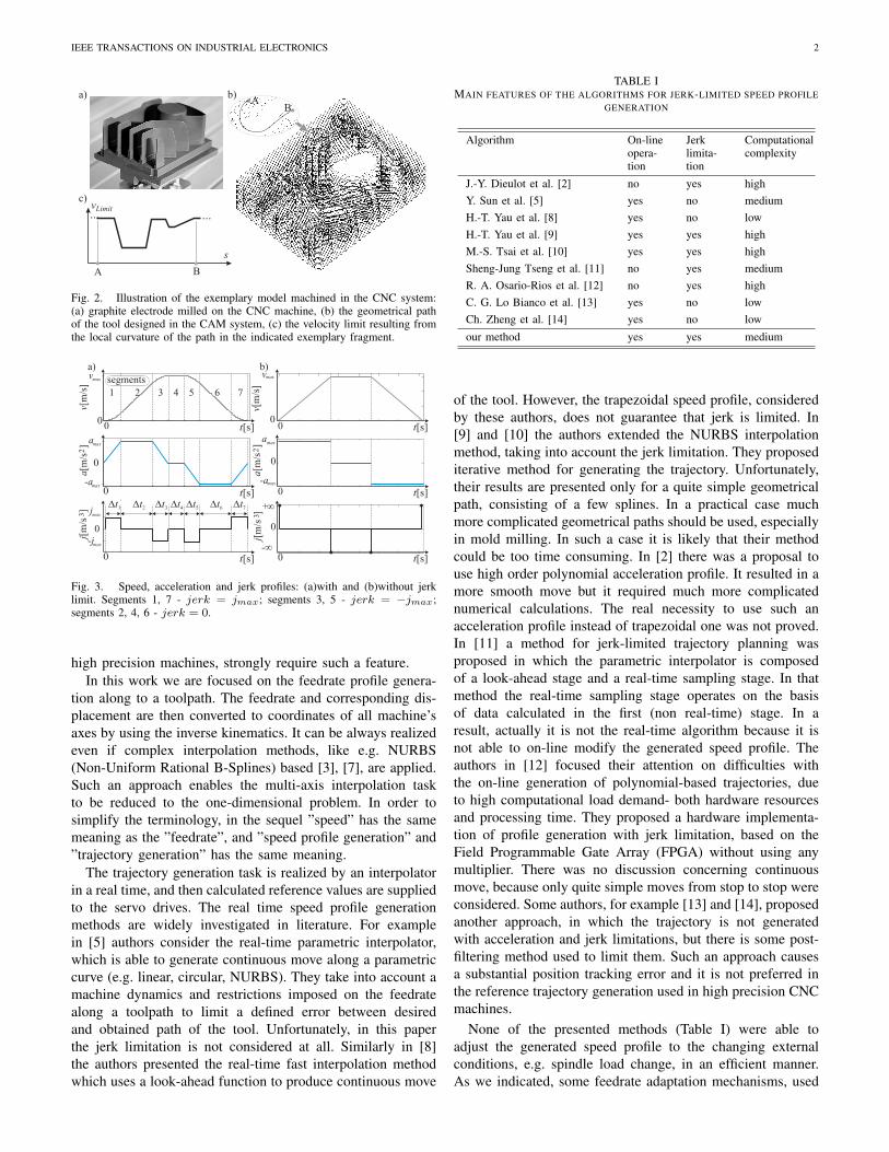
Any control system of a CNC machine should control theservo drives in such a way, that the feedrate is as closeas possible to the demanded value, and simultaneously thedefined speed limits are not violated. Moreover, the generatedtrajectory should be smooth, to avoid exciting the naturalfrequencies of the machine. The smooth trajectory can beobtained by imposing limits on the first and second timederivatives of feedrate, resulting in trapezoidal accelerationprofiles (Fig. 3.a). In Fig. 3.b a trapezoidal speed profile isshown. It is very popular and widely used because of itssimplicity. Unfortunately, it does not guarantee a high qualityof the machining because of discontinuities in accelerationreference values. In the other case, if a smooth speed profileis used (Fig. 3.a), the acceleration profile has no discontinuityand its trapezoidal form results from jerk limit. The sevensegments of that speed profile have maximal, minimal or zerovalues of the jerk. The trajectory presented in Fig. 3.a describesa simple move from stop to stop, but if a more complexmove is used (i.e. continuous move without stops) then thesesegments may occur in different sequences and/or amounts.

The on-line speed profile generation methods are widelyinvestigated in literature [2]-[6]. Unfortunately, none of thereported methods were able to adjust on-line the generatedspeed profile to the changing external conditions with simul-taneous limitation of the value of the jerk. However, it shouldbe emphasized that feedrate adaptation mechanisms, used in

Accepted for publication in IEEE Transactionson Industrial Electronics − 2012


AB

A B

s

vLimit

... ...

a) b)

c)

Fig. 2. Illustration of the exemplary model machined in the CNC system:(a) graphite electrode milled on the CNC machine, (b) the geometrical pathof the tool designed in the CAM system, (c) the velocity limit resulting fromthe local curvature of the path in the indicated exemplary fragment.

¥

¥

0

0

0

0

a[m

/s ]

00

v[m

/s]

0

j [m

/s ]

j[m

/s ]

-

+

0

0

0

Dt1 Dt2 Dt3 Dt4 Dt5 Dt6 Dt7

t[s]

t[s] t[s]

t[s]

t[s]

a[m

/s ]

a a

-a -a

v v

j

-j

00

v[m

/s]

23

23

t[s]

a) b)

segments

1 2 3 4 5 6 7

max max

maxmax

maxmax

max

max

Fig. 3. Speed, acceleration and jerk profiles: (a)with and (b)without jerklimit. Segments 1, 7 - jerk = jmax; segments 3, 5 - jerk = −jmax;segments 2, 4, 6 - jerk = 0.

high precision machines, strongly require such a feature.In this work we are focused on the feedrate profile genera-

tion along to a toolpath. The feedrate and corresponding dis-placement are then converted to coordinates of all machine’saxes by using the inverse kinematics. It can be always realizedeven if complex interpolation methods, like e.g. NURBS(Non-Uniform Rational B-Splines) based [3], [7], are applied.Such an approach enables the multi-axis interpolation taskto be reduced to the one-dimensional problem. In order tosimplify the terminology, in the sequel ”speed” has the samemeaning as the ”feedrate”, and ”speed profile generation” and”trajectory generation” has the same meaning.

The trajectory generation task is realized by an interpolatorin a real time, and then calculated reference values are suppliedto the servo drives. The real time speed profile generationmethods are widely investigated in literature. For examplein [5] authors consider the real-time parametric interpolator,which is able to generate continuous move along a parametriccurve (e.g. linear, circular, NURBS). They take into account amachine dynamics and restrictions imposed on the feedratealong a toolpath to limit a defined error between desiredand obtained path of the tool. Unfortunately, in this paperthe jerk limitation is not considered at all. Similarly in [8]the authors presented the real-time fast interpolation methodwhich uses a look-ahead function to produce continuous move

TABLE IMAIN FEATURES OF THE ALGORITHMS FOR JERK-LIMITED SPEED PROFILE

GENERATION

Algorithm On-lineopera-tion

Jerklimita-tion

Computationalcomplexity

J.-Y. Dieulot et al. [2] no yes highY. Sun et al. [5] yes no mediumH.-T. Yau et al. [8] yes no lowH.-T. Yau et al. [9] yes yes highM.-S. Tsai et al. [10] yes yes highSheng-Jung Tseng et al. [11] no yes mediumR. A. Osario-Rios et al. [12] no yes highC. G. Lo Bianco et al. [13] yes no lowCh. Zheng et al. [14] yes no low

our method yes yes medium

of the tool. However, the trapezoidal speed profile, consideredby these authors, does not guarantee that jerk is limited. In[9] and [10] the authors extended the NURBS interpolationmethod, taking into account the jerk limitation. They proposediterative method for generating the trajectory. Unfortunately,their results are presented only for a quite simple geometricalpath, consisting of a few splines. In a practical case muchmore complicated geometrical paths should be used, especiallyin mold milling. In such a case it is likely that their methodcould be too time consuming. In [2] there was a proposal touse high order polynomial acceleration profile. It resulted in amore smooth move but it required much more complicatednumerical calculations. The real necessity to use such anacceleration profile instead of trapezoidal one was not proved.In [11] a method for jerk-limited trajectory planning wasproposed in which the parametric interpolator is composedof a look-ahead stage and a real-time sampling stage. In thatmethod the real-time sampling stage operates on the basisof data calculated in the first (non real-time) stage. In aresult, actually it is not the real-time algorithm because it isnot able to on-line modify the generated speed profile. Theauthors in [12] focused their attention on difficulties withthe on-line generation of polynomial-based trajectories, dueto high computational load demand- both hardware resourcesand processing time. They proposed a hardware implementa-tion of profile generation with jerk limitation, based on theField Programmable Gate Array (FPGA) without using anymultiplier. There was no discussion concerning continuousmove, because only quite simple moves from stop to stop wereconsidered. Some authors, for example [13] and [14], proposedanother approach, in which the trajectory is not generatedwith acceleration and jerk limitations, but there is some post-filtering method used to limit them. Such an approach causesa substantial position tracking error and it is not preferred inthe reference trajectory generation used in high precision CNCmachines.

None of the presented methods (Table I) were able toadjust the generated speed profile to the changing externalconditions, e.g. spindle load change, in an efficient manner.As we indicated, some feedrate adaptation mechanisms, used


in high precision machines, require such a feature. Moreover,if a very complicated CAM model is machining, it is possiblethat the internal memory of the interpolator has not enoughcapacity to hold the whole path. In such a case the workmust be divided into separate parts, what is unfavorable. Thesolution is to treat the limited memory of the interpolator as adynamic buffer, which can be filling up while the machine isworking. The incoming new data should be taken into accountin the on-line trajectory generation method, because of anecessity to generate the continuous work without unnecessarystops.

In the paper the on-line speed profile generation methodwill be developed by making use of a flexible neuro-fuzzysystem proposed and studied in [15]-[18]. In our investigationsit is very important to achieve a very high accuracy of anapproximation at a certain stage of on-line speed profile gen-eration and the flexible neuro-fuzzy approximator satisfied ourrequirements. It should be noted that neuro-fuzzy structurescombine the advantages of neural networks and classical fuzzysystems and are frequently applied to solve various problemsof control, process modeling and fault diagnosis [4], [19]-[26].We will develop a new method for efficient generation of asmooth velocity profile for CNC machines. The unique featureof our method, which is distinguished from other solutions,is the ability to quickly adjust the generated trajectory tochanging speed limits. In our approach it is possible tomodify the demanded value of the feed rate of the tool duringmachine operation. This feature is very important for operatingCNC machines because of the need to protect the cutterfrom the brake and spindle from the overload in high speedmachining. To our best knowledge the approach presentedin this paper is the only method providing the efficient on-line smooth speed profile generator in milling machines. Theidea of a new method for the on-line trajectory generationis described in Section II. In Section III.A we describe theflexible Takagi-Sugeno neuro-fuzzy system used for the speedprofile generation, whereas Section III.B presents simulationresults. Conclusions are given in Section IV.

II. A NEW ALGORITHM FOR ON-LINE TRAJECTORYGENERATION

Our method is based on the proposed in this paper originalconcept of test trajectories (Fig. 4) which are generated infixed time periods TG.

A. Main idea

The interpolation of a displacement, speed and accelerationas a function of time tL, with the jerk limitation, is based onthe well known motion equations

a (tL) = a0 + j0 · tL, (1)

v (tL) = v0 + a0 · tL + j0 ·t2L2, (2)

and

k= , ,...1 2

Violating test trajectories

v

v

ss

a)

c) d)ss

v

v

Non-violating test trajectories Resultant trajectory

First (safe) trajectory

First test trajectory

First predicted

state =[ ]IP P P P

s , v , a1 1 1 1

k-th test trajectory

k-th safe trajectory

k

s , v , a

-th predicted

state =[ ]IP P P P

k k k k

1 1 1 1

b)

k k k k

First current state

[ ]IC C

= s , v , aC C

k

= s , v , a

-th current state

[ ]IC C C C

Fig. 4. Method for the on-line generation of the jerk limited trajectory(thick gray curve) taking into account the feedrate limitation (thick blackcurve). Thin gray and black curves represent test trajectories, violating andnot violating velocity limitation, respectively, along corresponding distance.

s (tL) = s0 + v0 · tL + a0 ·t2L2

+ j0 ·t3L6, (3)

where j0 is an applied value of the jerk, and (4) fully definesthe interpolator state

s = [s, v, a], (4)

where subscript zero denotes values at a moment of a relativetime tL = 0. Based on equations (1)-(3), the on-line speedprofile generator is designed. The detailed flowchart of ouralgorithm is presented in Fig. 5 and Fig. 9.

The interpolation is always based on a basis of a knowncurrent interpolator state

ICk =[sCk , v

Ck , a

Ck

](5)

and an initially known safe trajectory (step A3 in Fig. 5) whichis shown in Fig. 4.a. The trajectory is defined by a set ofstarting values

TSk =

{∆tSk,1, s

Sk,1, v

Sk,1, a

Sk,1

}, . . . ,{

∆tSk,7, sSk,7, v

Sk,7, a

Sk,7

} , (6)

i.e.: displacement s, velocity v, acceleration a, jerk j and valueof the time period ∆t for seven successive segments as it isshown in Fig. 6. The safe trajectory guides the CNC machinefrom the starting point to the stop, guarantying the velocity,acceleration and jerk limitations.

We can easily predict (step A4 in Fig. 5) a future state of theinterpolator (in a time distance TG from the current moment)along the safe trajectory

IPk =[sPk , v

Pk , a

Pk

]. (7)

Treating this predicted state as a starting point we can generateone test trajectory (step A7 in Fig. 5), defined by the followingset of parameters

TTk =

{∆tTk,1, s

Tk,1, v

Tk,1, a

Tk,1

}, . . . ,{

∆tTk,7, sTk,7, v

Tk,7, a

Tk,7

} . (8)


he data describing theStep A1. Load t velocity speed limitalong a toolpath, in a form of sets of parameters of a first-degree polynomials for every ( = 1,2, ... ) short block:q Q

L=[ {sL1

,vL1

},{sL2,vL

2},...{sL

q,vL

q},...{sL

Q,v L

Q} ].

Start the indexing of these blocks: :=1q

Start the online speed profile generator

Step A4.Increment index value:k:=k+1 and generate thepredicted interpolator state IP

k=[s P

k,v P

k,aP

k], valid after time

TG

relative to the current interpolator state ICk

Step A7.Calculate the parameters for the next test trajectory:

TT

k=[ { sT

k,1, vT

k,1, aT

k,1,DtT

k,1}, ... {sT

k,7, vT

k,7, aT

k,7, DtTk,7

which starts from the previously predicted interpolator state IPk

Step A8.Does the testtrajectory violate the speed limit?Call the function (Fig. 9):ValidationOfTheTestTrajectory(L, TT

k)

==true?

Step A3.Start the indexing of the generated testtrajectories (k=0) and calculate the parameters of the firstsafe trajectory, in a form of TS

1=[ { ss

1,1,v s

1,1 ,as

1,1, Dt s

1,1},

... {ss1,7

,vsk,7 ,

as1,7

,Dts1,7

} ], starting from the knowninterpolator state I

Ck

Step A11.Acceptanceof the test trajectory as a new safetrajectory: TS

k := TTk

Updating of the interpolator state: ICk

:= IPk

Step A2.Enter the starting values for the interpolator stateIC

1=[sC

1,vC

1,aC

1]=[0,0,0]

Step A5. Check the stop

condition:sPk >sL

Q

Step A6.Stop profile generator

Start the Interpolator

Step A10.Synchronization with the real time interpolator(waiting for the start of the next TG cycle)

Step A9.

TG cycle Y

Y

Step B1. Start newTG

cycle.Set the relative time value t

L=0

Step B5. Stopinterpolator

Step B3. Checkthe stop condition

s>sLQ ?

Y

Step B2. Interpolation of a refference signals (s, v, a) at a

moment of relative time tL on a basis of motion equations(1)-(3)and the current safe trajectory paramsTS

k

Step B4. Synchronize with a real time clock and increase

the relative time value tL:=tL+DtL

Step B6.tL < TG ?

Y

N

Syn

ch

ron

izati

on

} ],

Waiting for thestart of the next

N

N

Fig. 5. Algorithm for generating test trajectories.

The test trajectory has the task to speed up the move alittle bit - comparing with the move resulted from the safetrajectory (Fig. 7). This speed up can be is easily done byapplying a non zero time period (∆tT1 ,∆tT2 ,∆tT3 ) values in aseven segments speed profile. In our case sum of these threeparameters was chosen experimentally and is equal to the valueof parameter TG. After this time interval the move should beimmediately slowing down to the stop, in a way defined byseven segments trajectory, using segments marked as 5, 6 and7 (Fig. 3.a). The calculations required to determine parameters

ss

k, 1 sk, 2 s

k, 3 sk, 4 s

k, 7sk, 6

t

t

v

v

vk, 1

vk, 3

vk, 4 v

k, 5

vk, 6

vk, 7

sk, 2

sk, 4

sk, 5

sk, 6

sk, 7

vk, 2

sk, 3

s

sk, 1

b)

c)

d)

sk, 5

vk, 1

vk, 2 v

k, 3

vk, 4

vk, 5

vk, 6

vk, 7

Dtk,1Dt

k,2 Dtk, 3 Dt

k,4

T

Dtk, 5 Dt

k, 7Dtk, 6

t

a ak, 1

ak, 2 a

k, 3ak, 4 a

k, 5

ak, 7

a)

ak, 6

Fig. 6. Example of the seven segments trajectory, defined by a set of startingvalues: a)acceleration as a function of time, b)velocity as a function of time,c)displacement as a function of time, d)velocity as a function of displacement.

of seven segments trajectory are widely presented in literature[1], [27]-[29] and will not be presented here.

The generated test trajectory has to be validated (step A8 inFig. 5 and Fig. 9), to determine if it violates or not the velocitylimit along the toolpath (thick black curve in Fig. 4). The speedlimit depends on the local curvature of the geometrical pathdesigned by a CAM system [1] and this dependency can beapproximated by any piecewise function, for example by thezero or higher order polynomial [28]. In this paper we usethe first order polynomial described by the following sets ofreference knots (Fig. 2c and Fig. 7)

L =

[ {sL1 , v

L1

},{sL2 , v

L2

}, . . . ,{

sLq , vLq

}, . . . ,

{sLQ, v

LQ

} ], (9)

which gives satisfactory compromise between accuracy andcomputational complexity. The number of blocks Q of such apiecewise curve depends on the complexity and length of thegeometrical path. In our work we assume that the piecewisecurve was determined in advance by a separate algorithm [8]that will not be discussed in this paper.

If a validation algorithm determines that the test trajectoryviolates the speed limit, this trajectory will be discarded (thingray curve in Fig. 4) what is shown in the block diagramas step A9. Otherwise, this trajectory will be the new safetrajectory, valid after TG time period (steps A10 and A11 inFig. 5). This procedure is repeated in successive time periodsand consecutive test trajectories are generated, each startingfrom the new working point (Fig. 4.b, Fig. 4.c). The finalsmooth speed profile (Fig. 4.d) is formed by a merger of shortsubsequent fragments of the safe trajectory.

Simultaneously, in a real time, with generating and validat-ing the test trajectories, a motion controller is working (stepsB1-B6). It performs the interpolation of a displacement, speedand acceleration along a tool path in the fixed time steps ∆tL.At this point the proper (adequate) inverse kinematics is alsoused to generate the reference values for all machine’s servo


0s

end of test trajectory

q Q=end of the path

the first (safe) trajectory

T - test trajectoryS - save trajectory

q=2

L - velocity limit

...

s "N

sk, 1T sk, 2

T sk, 3T s =sk, k, 54

T sk, 7T

s 'N

q=1

r=2 r=3

r=7

sC

s = ... sL 0 D

I1C

sk, 6T

v

I1P

0

q=3q=4

vL0

vL1

q=5

sQs1

L s2L s3

L s4L s5

L L

DsA

DsT

DsL

[ , , ]v a j0 0 0

T

I =S

r=1

r=4r=5 r=6

Fig. 7. Example of a test trajectory as a function of distance and intersectionsof its segments with speed constraints blocks. Grey area shows the currentlyanalyzed sectors in the iterative validation algorithm of the test trajectory.

drives. This method is commonly known [29], [30] and willnot be presented in this paper.

B. Method of validation of the test trajectory

In our system the validation algorithm of a test trajectory(Fig. 9) plays a key role. Analytical solution of such a taskis very complicated, because velocity constraints are linearfunctions of a displacement given by

vLimit (sL) = vL0 + (vL1 − vL0) ·sL∆s

, (10)

where

sL = ⟨0 . . .∆s⟩ , (11)

and vL0, vL1 are parameters of currently analyzed sector∆s, resulting from the velocity constraint curve (Fig. 7), tLand sL are time and position relative to the origin of theconsidered sector (gray area in Fig. 7), while generated speedand displacement profile are polynomial functions of time,given by (2) and (3).

Note that in Fig. 6.d as well as in Fig. 7 the velocity profilesare shown as a function of a displacement. Creating thesefigures was only possible on a basis of a performed iterativesimulation.

It is clear that the validation of the test trajectory can notbe done in one step. The velocity limit curve and the testtrajectory are defined in blocks or segments, respectively. Asa result the validation algorithm must be an iterative, withthe number of the iterations resulting from the number ofblocks of the limit curve and values of parameters of thetest trajectory. A length of currently analyzed sector (∆s)in successive iterations results from an intersection of thetrajectory segments and the speed constraints blocks (Fig. 7).Analyzed sectors must be iterated in such a way that theydo not cross the boundaries resulting from the blocks of thevelocity limit curve and the segments of the test trajectory.

Our method, which is based on a quadratic approximation ofthe test trajectory, requires to satisfy the following limitation;the value of ∆s cannot be greater than parameter ∆sA,which is explained in the sequel in this section, otherwise theapproximation accuracy will be poor. As a result the sector’s

length is determined as a minimal value of three values (∆sA,∆sT , ∆sL), as it is shown in Fig. 7, i.e.

∆s = min(∆sA,∆sT ,∆sL). (12)

Appropriate iterations to determine ∆s are shown in Fig. 9 assteps C2-C6 and steps C13-C18.

To validate the whole test trajectory, all successive sectorsmust be tested until the trajectory segments (8) end (step C19in Fig. 9). If any of the tested sectors violates the speed limit

v (sL) ≤ vLimit (sL) , sL ∈< 0, . . . ,∆s >, (13)

where

v (sL) = v (sL, v0, a0, j0) , (14)

then the whole tested trajectory must be discarded (step C12in Fig. 9)

In order to check analytically if the test trajectory at agiven sector violates or not the speed limit, we should haveit in a form of a function of the displacement. Unfortunately,there is no simple analytical projection, converting the testtrajectory from a function of time (Fig. 6.b) to a function ofdistance (Fig. 6.d). It results from the fact that equation (14)is an implicit function. Therefore, we propose a neuro-fuzzystructure to build an efficient validation system checking if thetest trajectory violates the velocity limit. More precisely, wedevelop the algorithm, depicted in Fig. 8, in which the neuro-fuzzy structure efficiently aids the quadratic approximationgiven by

v (sL) ≈ vA (sL) = C0+C1 ·sL+C2 ·s2L, sL ∈< 0, . . . ,∆s >(15)

of function (14). The neuro-fuzzy system is used in ourconcept to aid the classical quadratic approximation of thespeed profile, but not to directly approximate this profile.Such an approximated function reduces mentioned earliercomplex calculation, checking condition (13), to a simple taskof solving a quadratic inequality, related to checking conditiongiven by

vA (sL) ≤ vLimit (sL) , sL ∈< 0, . . . ,∆s > . (16)

The effective method of determining the coefficients ofequation (15) with the help of neuro-fuzzy system will bepresented in the following part of this section.

The quadratic approximation of function (14) is alwayspossible with a defined maximum acceptable approximationerror ( vE < vEmax in Fig. 10), if the approximation distance∆s does not exceeds ∆sA, which depends on the currentcurvature of the approximated function (14). The value of∆sA, depends on the three parameters, i.e.

∆sA = ∆sA (v0, a0, j0) , (17)

which fully defines the interpolator state at the origin of theanalyzed sector (Fig. 7).

Unfortunately, this dependency is not known in advance andcan only be obtained by the trial and error method, based on


C , C C v v0 1 2 0 1and - determine based on , vH and

- determine based on the , and the e uation (2)T T1 Hv v1 H, q

T T1 H, the bisection method- determine based on

Ds - determine based on formula (12)

DsA - determine based on the by three neuro-v0 0 0, , , fuzzy

systems, which were trained with data obtainedfrom the offline trial and error method

a j

Fig. 8. Flowchart illustrating how the neuro-fuzzy structure efficientlyaids the quadratic approximation of the test trajectory, as a function of thedisplacement in the subsequent segments.

many repeated iterative simulations, with an usage of motionequations (1)-(3). Because the trial and error method is verytime consuming, it is not suitable to use in the validationsystem. Fortunately, we can use the neuro-fuzzy structure toapproximate dependency (17) in an efficient manner.

Finally, if we know the value of ∆sA, we can approximatefunction (14) in the form of (15) making additional analyticalcalculations, resulting from the use of Dirichlet boundaryconditions, i.e.:

C0 = v0, (18)

C1 = −3 · v0 + v1 − 4 · vH∆s

(19)

and

C2 =2 · v0 + 2 · v1 − 4 · vH

∆s2. (20)

The proposed in this paper boundary conditions require theequality of the values of the approximated function (14) andtheir quadratic approximation (15) at the start point (v0), halfpoint (vH ) and end point (v1) of the approximation distance∆s (Fig. 10). The velocity v0 at the origin of the sector isalready known (Fig. 7), but the value of vH and value of v1are not known and should be determined here. At first thecorresponding values of the relative times (∆TH ) and (∆T1)must be determined. It can be easily done by a commonlyknown bisection method with the utilization of the motionequation (3) and the values of the interpolator state describedby

IS = [s0, v0, a0] (21)

at the origin of analyzed sector. The move defined by the testtrajectory is progressive (i.e. v (tL) ≥ 0) within consideredrange, so the bisection method with over a dozen simpleiterations is sufficient to obtain satisfactory accuracy (step C8in Fig. 9). In the bisection method the maximum value of∆Tmax for search algorithm is set to a minimal positive valueof relative time, at which the velocity described by formula(2), reaches the value equal to zero. If the velocity does notreach the zero for any positive value of the relative time, then

Estimation ofthe maxsector's length

Start ValidationOfTheTestTrajectory(L, TTk)

Step C1. Enter starting values of local variables:

r :=1, s0:=sT

k,r, v

0:=vT

k,r, a

0:=aT

k,r

Steps C2,3. Compute sN’ := sT

k,r+1; DsT=s

N’-s

0

Step C6. Find the sector’s length: Ds := min(DsT , DsL, DsA)

Step C7. Calculate the local parameters of the the velocity limit L

q

Step C17. Switch to the next

segment of the test trajectory:

0s :=s

N’

v0:=vT

k,r+1

0 ,ra :=aT

k +1

r := r+1

Step C18. Updating values of the local variables

s0:=s

0+Ds v0 := v0+a0•T1 +j0•T1

2 /2 a0:=a

0+j

0•T

1

Y

N

YStep C14. Check the stop condition:End of the segments of the test trajectory?

sN’’ := sLq+1; DsL=sN”-s0

Step C5b. j0=+jmax; DsA =NF1(v0, a0)

Step C5c. j0=-jmax; DsA =NF3(v0, a0)

Step C5a. j0=0; DsA =NF2(v0, a0)

Step C4. Select

the appropriate

jerk value

Step C8. Compute the local variables (T1, TH) using the bisectionmethod and the motion equations at known starting values:v

0,a

0, j

0:

- time to reach the given displacementT , T1 H D Ds and s/2, respectively

T1

:=CalculateTDs(Ds, v0, a

0j0);

,

TH :=CalculateTDs(Ds/2, v0, a0, j0)

Step C10. Calculate the parameters C0, C1, C2 (18)-(20) of thequadratic equation (15)

Step C11. Is there at least one real root of the quadratic equation

(16) in the range [0..DS], or total time duration limit is reached ?

Y

Step C15. Does theend of the sector

indicate the next block

of the velocity limitcurve L?

(sN’<s

N”) and

( ” D AsN <s0+ s )?N

Step C16. Switch to a next block of

the velocity limit curve q:=q+1

Step C9. Calculate the auxiliary local variables v1

and vH

-

velocities at a given point of the test trajectory tL=T

1and t

L=T

H,

respectively, based on the motion equations (2)

Designation of the next sector to check

r=1 or r=7 ? r=2 or r=4 or r=6 ?

r=3

r=5?or

YY

r >6 ?

Step C19. Return false

Quadratic approximation of the analysed sector

VL 0

= vL + tangVL

•(s0

- sL )

tangVL

:=(vLq+1

- vLq

)/(s Lq+1

- sL )q

q VL 1 = VL 0 + tangVL•Ds;

Checking the speed limit violationand the total duration time limit of the validation process

Step C12. Return true

Y

Step C13. Does the end of the sector indicate a newsegment of the trajectory? (s

N’<s

N”) and (s

N’ <s

0+DsA )?

the auxiliary values:

Fig. 9. Flowchart illustrating validation of the test trajectory.

value of ∆Tmax is set to reasonable limit equal to one second.The minimal value for search algorithm is set to zero.

If the values of (∆TH ) and (∆T1) are calculated, thenthe values of vH and v1 can be easily determined (step C9)on a basis of the motion equation (2). Finally at step C10of the presented algorithm, parameters C0, C1 and C2 of


v1

vH

v0

v (s )Lv (s )L

A

( ) ( )| |max0...

max

L

A

E E L Ls s

v v v s v sÎ D

> = -

sL0 Ds1 Ds/2

Fig. 10. Quadratic approximation of a velocity profile as a function ofdisplacement.

the quadratic function (15) can be simply calculated usingformulas (18)-(20). As a result we can use the quadraticinequality (16) instead of the complicated formula (13) whichsignificantly simplifies the trajectory validation algorithm. Inthe next step (C11) we should solve the quadratic inequality(16) to check whether the analyzed sector of the test trajectoryviolates or not the speed limit. It can be easily done bychecking if the adequate quadratic equation has at least onereal root in the range [0,∆s]. Because v0 has always valueless than vL0 (Fig. 7), the real root within a range [0,∆s] isthe velocity violation point. As it was previously explained,in such a case validation of the test trajectory is completed(step C12) with a result equal to true. This procedure is alsoterminated with a result equal to true if the total duration timelimit (TG) of the validation procedure is reached. In anothercase the steps C13-C19 are performed to switch to the nextsector in the iterative validation algorithm.

III. FLEXIBLE TAKAGI-SUGENO NEURO-FUZZY SYSTEMFOR THE SPEED PROFILE GENERATION

A. Description of the system

The flexible Takagi-Sugeno neuro-fuzzy approximator isan important part of the proposed in the paper an originalalgorithm or the on-line speed profile generation. It allows toimplement our approach in a typical real-time controller andto eliminate the lookup table method, which cannot be usedbecause of the limited amount of the memory.

In the last decade different structures of neuro-fuzzy net-works have been presented, often referred to in the worldliterature as neuro-fuzzy systems [6], [15], [17], [18]. As itwas indicated in the Introduction, they combine the advantagesof neural networks and classical fuzzy systems. In particular,the neuro-fuzzy networks are characterized - in contrast withneural networks - by a interpretable representation of knowl-edge represented by fuzzy rules. As generally known, theknowledge in neural networks is represented by the values ofsynaptic weights, and therefore is completely not interpretable,for instance, for a user of a medical expert system basedon neural networks. Moreover, neuro-fuzzy networks can betrained, using the idea of error backpropagation method, whichis the basis of learning of multilayer neural networks. Thelearning usually applies to membership function parametersof the IF and THEN parts of the fuzzy rules. It should beemphasized that neuro-fuzzy systems are universal approxi-mators.

The advantages of neuro-fuzzy networks are the reason fortheir common application in classification, approximation andprediction problems. Most of neuro-fuzzy structures describedin the world literature utilizes the Mamdani type inferenceor the Takagi-Sugeno schema. The Mamdani type inferenceconsists in connecting the antecedents and the consequents ofrules using a t-norm (most often the t-norm of the min type orof the product type). Then the aggregation of particular rules ismade using a t-conorm. In case of the Takagi-Sugeno schema,the consequents of the rules are not fuzzy in nature, but arefunctions of the input variables. Less often the logical infer-ence is applied, which consists in connecting the antecedentsand the consequents of rules using a fuzzy implication thatsatisfies the conditions of definition of fuzzy implication.In case of an inference of logical type the aggregation ofparticular rules is made using a t-conorm [17], [18].

It is well know [18] that introducing additional parametersto be tuned in neuro fuzzy systems improves their performanceand they are able to better represent the patterns encoded inthe data. Therefore, in this paper, we incorporate flexibilityconcepts into the neuro-fuzzy system: certainty weights to theaggregation of rules and to the connectives of antecedents.

The flexible neuro-fuzzy system was used in our methodbecause it is an excellent tool for solving approximationproblems. However, alternatively other techniques (e.g. neuralnetworks), can be incorporated into scheme depicted in Fig.9, instead of flexible neuro-fuzzy systems. The novelty of ourapproach lies in developing the original algorithm for speedprofile generation, by using the concept of the test trajectories,rather than in developing an approximator.

The algorithm in Fig. 9 uses the flexible neuro-fuzzy Takagi-Sugeno system. The neuro-fuzzy system determines the max-imum value of the sector’s length (steps C5a-C5c in Fig. 9),for which the quadratic approximation of the trajectory at k-thstep is possible with an accuracy not worse than vEmax (Fig.10)). The neuro-fuzzy system determines the value of ∆sA

(Fig. 12 and Fig. 8) for current values of v0, a0, and for givenvalues of jerk (j0 = −jmax, j0 = 0, j0 = +jmax).

We will apply the two-input and single-output flexibleTakagi-Sugeno neuro-fuzzy system mapping X → Y, whereX ⊂ R2 and Y ⊂ R. The rule base is given by

R(r) :

IF x1 isA

r1

(wτ

1,r

)AND x2 isA

r2

(wτ

2,r

)THEN

f (r) (x) = cf0,r +2∑

i=1

cfi,rxi

(wdef

r

), (22)

where r = 1, 2, . . . , N . The construction of the system isbased on the following parameters and weights:

- parameters of membership functions µAki(xi), i = 1, 2,

r = 1, 2, . . . , N ,- parameters cf0,r, cfi,r, i = 1, 2, r = 1, 2, . . . , N , in linearmodels describing consequences,

- certainty weights wτi,r ∈ [0, 1], i = 1, 2, r = 1, 2, . . . , N ,

describing importance of antecedents in the rules,- certainty weights wdef

r ∈ R, r = 1, 2, . . . , N , describingimportance of the rules.


( )xAm

.

.

.

( )x

( )x

( )x1f

.

.

.

( )x2

f

( )xN

f

1x

2x

ydef

1

Am 2

Am N

Fig. 11. Flexible Takagi-Sugeno neuro-fuzzy system used for the validationof the test trajectory.

The aggregation in the Takagi-Sugeno model, described bythe rule base (22), is in the form

y = f (x) =

N∑r=1

wdefr · f (r) (x) · µAr (x)

N∑r=1

µAr (x)

, (23)

where

µAr (x) = T ∗ {µAr1(x1) , µAr

2(x2) ;w

τ1,r, w

τ2,r

}(24)

and T ∗ is a weighted t-norm [17], [18]. Weighted t-norm inthe two-dimensional case is defined as follows

T ∗{

µAr1(x1) , µAr

2(x2) ;

wτ1,r, w

τ2,r

}=

T

{1 +

(µAr

1(x1)− 1

)· wτ

1,r,1 +

(µAr

2(x2)− 1

)· wτ

2,r

} . (25)

The weights wτ1,r and wτ

2,r are certainties (credibilities) of bothantecedents in (25). Observe that:

- If wτ1,r = wτ

2,r = 1 then the weighted t-norm is reducedto the standard t-norm.

- If wτ1,r = 0 then T ∗ {µAr

1(x1) , µAr

2(x2) ; 0, w

τ2,r

}=

1 +(µAr

2(x2)− 1

)· wτ

2,r.The general architecture of the flexible Takagi-Sugeno sys-

tem is depicted in Fig. 11. As we can see, it is a multilayernetwork structure. To train it, the idea of the error backprop-agation method may be applied [17], [18]. Let us define thelearning sequence as (x1,d1) , (x2,d2) , . . . , (xZ ,dZ), wherexz = [v0z, a0z], dz =

[∆sAz

], z = 1, 2, . . . , Z. Based on the

learning sequence we determine all parameters and weights offuzzy system (23).

B. Experimental results

The neuro-fuzzy structure (23) aids the validation algorithmused in the trajectory generation system. This system is usedas an approximator of the highly nonlinear dependency (17).Because the jerk can have only three discrete values (Fig. 3.a),we can use three simple neuro-fuzzy system for these threeseparate cases instead of a complex one. In that case each ofthe three neuro-fuzzy systems approximate a highly nonlinearfunction (Fig. 12) for different values of the jerk (steps C5a,C5b and C5c in Fig. 9). We use neuro-fuzzy system NFS1given by

0

0.4

-5

50

10

0

0.4

-5

50

10

a) b)

v [m/s] v [m/s]

Ds [mm] Ds [mm]

a [m/s ]20 0a [m/s ]20 0

AA

Fig. 12. Graphical representation of ∆sA obtained from simulations as afunction of velocity and acceleration at given values of the jerk: a)j0 = 0,b)j0 = 250.

∆sA = NFS1 (v0, a0) , (26)

when we analyze segments r = 1, 7, neuro-fuzzy system NFS2given by

∆sA = NFS2 (v0, a0) (27)

for segments r = 2, 4, 6 or neuro-fuzzy system NFS3 givenby

∆sA = NFS3 (v0, a0) , (28)

for segments r=3, 5.A minor disadvantage of such a simplification is the neces-

sity to declare the value of jmax at the stage of designing thecontrol system, in principle before training the neuro-fuzzysystem. This is not a big drawback because the value of jmax

is never changed during the entire use of the machine. Theselection and fixing the value of the jmax as well as theinitial tuning phase of the used neuro-fuzzy system must bedone only once, at the stage of designing the system. It ispossible to prepare several flexible neuro-fuzzy systems, eachlearned in advance (for different values of the jmax typicallyused in practice) and use them later without modification. Thesignificant advantage of such an approach is the simplificationof the neuro-fuzzy system and the whole algorithm is moreefficient in a real time implementation.

Three independent flexible neuro-fuzzy Takagi-Sugeno sys-tems were prepared for the verification of the test trajectory(steps C5a-C5c in Fig. 9). Each of these systems (26)-(28) determines the output ∆sA for another jerk j0 fromthe set {−jmax, 0,+jmax}. Training data, which were usedin the learning process, were generated by trial and errormethod. The idea of generate the training data was based onthe assumption, that the outputs ∆sA, should have greatervalues, what results in decreasing number of steps valida-tion algorithm of a test trajectory. Obviously, the conditionVE < VEmax should be satisfied (Fig. 10).

We used neuro-fuzzy systems given by (23) characterizedby the Gaussian fuzzy sets, 30 rules (N = 30) and algebraict-norms. We employed the Fuzzy C-Mans algorithm to findinitial values of membership functions parameters (m = 2.0,1000 steps) [15], [17], [18]. We also initialized weights ofantecedents wτ

i,r = 1, i = 1, 2, r = 1, 2 . . . , N , and weightsof the rules wagr

r = 1, r = 1, 2 . . . , N . The learning datalength for each of three neuro-fuzzy systems (26)-(28) was


s [mm]20 40

1[mm/s]a)

5[mm/s]

60 70

b)

c)5[mm/s]

Startthe demanded speed

decreasing

503010

v [mm/s]

100

d)

Fig. 13. The velocity limit (thick black), the smooth trajectory obtained withthe three neuro-fuzzy systems (thin black), and the smooth trajectory obtainedwith the trial and errors method (gray).

Z = 1682. The system was learned by the backpropagationmethod (µ = 0.15) with momentum (λ = 0.10) by 100000epochs. The final average root mean square error (RMSE)was equal 0.0996 for three used neuro-fuzzy systems. Ourapproach allows to easily implement the presented algorithmin a microprocessor system used in the CNC machine.

The final trajectory obtained with the help of the threeneuro-fuzzy systems (26)-(28) is shown in Fig. 13. Thecomparison with the trajectory obtained by the trial and errorsmethod shows that there are some insignificant differencesbetween them, resulting from the neuro-fuzzy systems approx-imation errors. Despite the slight differences between thesetwo cases, the ”neuro-fuzzy based” trajectory fully guaranteesthe required limits of jerk, acceleration and velocity, and inresult it is suitable to use in the CNC system.

In Fig. 13 some areas are enlarged to better illustratethe specific features of the presented algorithm. In the firstindicated area (Fig. 13.a) the small velocity fluctuations arevisible. It results from the fact, that the final trajectory isformed by a merger of short fragments of the successive testtrajectories. Generally this is a drawback of the presentedalgorithm. However, if the amplitudes of these fluctuationsare small, then it does not influence negatively on the qualityof the work. Their amplitude is proportional to the lengthof the connecting pieces, which depends in turn on the timeperiod TG used to generate and validate the subsequent testtrajectories. Decreasing this time period causes the reductionof the amplitude, but it requires more computational powerof the computer system. In our work we used TG withexperimentally chosen value equal to 2 milliseconds.

The next enlarged fragment (Fig. 13.b) shows that un-favorable slowdown occurs if the speed limit curve dropssharply. This drawback results from the lack of the globalvelocity optimization techniques. However, preprocessing ofthe velocity limit curve, i.e. eliminating the sharp drops, couldbe used to prevent that adverse slowdown (Fig. 13.c).

Despite of these minor drawbacks, a great advantage of ouralgorithm is that it is able to adjust the generated speed profileto the changing external conditions, e.g. spindle load change,in an efficient manner. As it was indicated in the Introduction,in our approach it is possible to modify the demanded valueof the feed rate of the tool during machine operation. This isillustrated in simulation presented in Fig. 13.d in which thespeed limit is decreased in order to protect the spindle from

the overload. As we can see, the algorithm is able to on-linemodify the generated speed profile.

IV. CONCLUSIONS

In this paper we presented a new algorithm for the on-line speed profile generation for industrial machine tool. Theunique feature of our method is the ability to quickly adjustthe generated trajectory to changing speed limits. It is possibleto modify the requested value of the feed rate of the toolduring machine operation. This feature is very importantfor operating CNC machines because of the need to protectthe cutter from the brake and spindle from the overload inhigh speed machining. Our method, based on the neuro-fuzzyapproach, allows the system to work properly and quickly,and to construct the trajectory generator operating on-line. Itshould be noted that neuro-fuzzy structures can be adopted forrealization in hardware, e.g. in the CMOS technology [31].

ACKNOWLEDGMENT

This paper was prepared under project operated within theFoundation for Polish Science Team Programme co-financedby the EU European Regional Development Fund, OperationalProgram Innovative Economy 2007-2013, Polish-SingaporeResearch Project 2008-2011 and also supported by NationalScience Center NCN.

The authors would like to thank the reviewers for veryhelpful suggestions and comments in the revision process.

REFERENCES

[1] M.-T. Lin, M.-S. Tsai, H.-T. Yau, Development of an dynamics-basedNURBS interpolator with real-time look-ahead algorithm, InternationalJournal of Machine Tools & Manufacture, vol. 47, pp.2246-2262, 2007.

[2] J.-Y. Dieulot, I. Thimoumi, F. Colas, R. Bare, Numerical aspects andperformances of trajectory planning methods of flexible axes, Interna-tional Journal of Computers, Communications & Control, vol. I, no. 4,pp. 35-44, 2006.

[3] W. T. Lei, M. P. Sung, L. Y. Lin, J. J. Huang, Fast real-time NURBS pathinterpolation for CNC machine tools, International Journal of MachineTools & Manufacture, vol. 47, pp.1530-1541, 2007.

[4] Fuchun Sun, Li Li, Han-Xiong Li, Huaping Liu, Neuro-Fuzzy Dynamic-Inversion-Based Adaptive Control for Robotic Manipulators-DiscreteTime Case, IEEE Transactions on Industrial Electronics, vol. 54, no.3, 2007, pp. 1342-1351.

[5] Y. Sun, J. Wang, D. Guo, Guide curve based interpolation scheme ofparametric curves for precision CNC machining, Parametric NURBSCurve Interpolators: A Review, International Journal of Machine Tools& Manufacture, vol. 46, pp. 235-242, 2006.

[6] T. Takagi and M. Sugeno. Fuzzy identification of systems and itsapplication to modeling and control, IEEE Trans. Syst., Man, Cybern.,vol. 15, pp. 116 132, 1985.

[7] S. Mohan, S.-H. Kweon1, D.-M. Lee1 and S.-H. Yang, ParametricNURBS curve interpolators: A Review, International Journal of Pre-cision Engineering and Manufacturing, vol. 9, no. 2, pp. 84-92, 2008.

[8] H.-T. Yau, J.-B. Wang, Fast Bezier interpolator with real-time lookaheadfunction for high-accuracy machining, International Journal of MachineTools & Manufacture,vol. 47, pp. 1518-1529, 2007.

[9] H.-T. Yau, J.-B. Wang, C.-Y. Hsu and C.-H- Yeh, PC-based controllerwith real-time look-ahead NURBS interpolator, Computer-Aided Design& Applications, vol. 4, 1-4, pp 331-340, 2007.

[10] M.-S. Tsai, H.-W. Nien, H.-T. Yau, Development of an integratedlook-ahead dynamics-based NURBS interpolator for high precisionmachinery, Computer-Aided Design, vol. 40, pp. 554-566, 2008.

[11] Sheng-Jung Tseng, Kuan-Yuan Lin, Jiing-Yih Lai, and Wen-Der Ueng, ANURBS curve interpolator with jerk-limited trajectory planning, Journalof the Chinese Institute of Engineers, vol. 32, no. 2, pp. 215-228, 2009.


[12] R. A. Osario-Rios, R. d. J. Romero-Trosncoso, G. Herera-Ruiz, R.Casteneda-Miranda, FPGA implementation of higher degree polynomialacceleration profiles for peak jerk reduction in servomotors, Roboticsand Computer-Integrated Manufacturing, vol. 25, pp. 379-392, 2009.

[13] C. G. Lo Bianco, R. Zanasi, Smooth profile generation for a tile printingmachine, IEEE Transactions on Industrial Electronics, vol. 50, No. 3,pp. 471-477, 2003.

[14] Ch. Zheng, Y. Su, P. C. Muller, Simple on-line smooth trajectorygeneration for industrial systems, Mechatronics, vol. 19, pp.571-576,2009.

[15] K. Cpałka, A New Method for design and reduction of neuro-fuzzyclassification systems, IEEE Transactions on Neural Networks, vol. 20,No. 4, 2009, pp. 701-714.

[16] L. Rutkowski, Flexible Neuro-Fuzzy Systems. Kluwer Academic Pub-lishers, 2004.

[17] L. Rutkowski and K. Cpałka, Designing and learning of adjustable quasitriangular norms with applications to neuro-fuzzy systems, IEEE Trans.Fuzzy Syst., vol. 13, no. 1, pp. 140-151, 2005.

[18] L. Rutkowski and K. Cpałka, Flexible neuro-fuzzy systems, IEEE Trans.Neural Networks, vol. 14, no. 3, pp. 554-574, 2003.

[19] B.K. Bose, N.R. Patel, K. Rajashekara, A neuro-fuzzy-based on-lineefficiency optimization control of a stator flux-oriented direct vector-controlled induction motor drive, IEEE Transactions on IndustrialElectronics, vol. 44, no. 2, 1997, pp. 270-273.

[20] A. Chatterjee, R. Chatterjee, F. Matsuno, T. Endo, Augmented StableFuzzy Control for Flexible Robotic Arm Using LMI Approach andNeuro-Fuzzy State Space Modeling, IEEE Transactions on IndustrialElectronics, vol. 55, no. 3, 2008, pp. 1256-1270.

[21] D. Fuessel, R. Isermann, Hierarchical motor diagnosis utilizing structuralknowledge and a self-learning neuro-fuzzy scheme, IEEE Transactionson Industrial Electronics, vol. 47, no. 5, 2000, pp. 1070-1077.

[22] P.Z. Grabowski, M.P. Kazmierkowski, B.K. Bose, F. Blaabjerg, A simpledirect-torque neuro-fuzzy control of PWM-inverter-fed induction motordrive, IEEE Transactions on Industrial Electronics, vol. 47, no. 4, 2000,pp. 863-870.

[23] P. Melin, O. Castillo, Intelligent control of complex electrochemicalsystems with a neuro-fuzzy-genetic approach, IEEE Transactions onIndustrial Electronics, vol. 48, no. 5, 2001, pp. 951-955.

[24] T. Orlowska-Kowalska, M. Dybkowski, K. Szabat, Adaptive Sliding-Mode Neuro-Fuzzy Control of the Two-Mass Induction Motor DriveWithout Mechanical Sensors, IEEE Transactions on Industrial Electron-ics, vol. 57, no. 2, 2010, pp. 553-564.

[25] T. Orlowska-Kowalska, K. Szabat, Control of the Drive System WithStiff and Elastic Couplings Using Adaptive Neuro-Fuzzy Approach,IEEE Transactions on Industrial Electronics, vol. 54, no. 1, 2007, pp.228-240.

[26] C.K. Kwong, K.Y. Chan, H. Wong, Takagi-Sugeno neural fuzzy model-ing approach to fluid dispensing for electronic packaging, Expert Systemswith Applications, vol. 34, issue 3, 2008, pp. 2111-2119.

[27] K. Erkorkmaz, Y. Altintas, High speed CNC system design. Part I: jerklimited trajectory generation and quintic spline interpolation, Interna-tional Journal of Machine Tools & Manufacture, vol. 41, pp.1323-1345,2001.

[28] N.Y. Ki, A new velocity profile generation for high efficiency CNCmachining application, City University of Hong Kong, Master Thesis,pp.1-83, 2008.

[29] S. Macfarlane, On-Line smooth trajectory planning for manipulators,The University of British Columbia, Master Thesis, pp.1-146, 2001.

[30] D. W. Pessen, Industrial automation. Circuit Design and Components,John Willey & Sons, Inc., pp.478-483, 1989.

[31] B.M. Wilamowski, R.C. Jaeger, M.O. Kaynak, Neuro-fuzzy architecturefor CMOS implementation, IEEE Transactions on Industrial Electronics,vol. 46, no. 6, pp. 1132-1136, 1999.

Leszek Rutkowski (F’05) received the M.Sc. andPh.D. degrees in 1977 and 1980, respectively, bothfrom the Technical University of Wroclaw, Poland.Since 1980, he has been with the Technical Uni-versity of Czestochowa where he is currently aProfessor and Chairman of the Computer Engi-neering Department. From 1987 to 1990 he helda visiting position in the School of Electrical andComputer Engineering at Oklahoma State Univer-sity. His research interests include neural networks,fuzzy systems, computational intelligence, pattern

classification and expert systems. In May and July 2004 he presented inthe IEEE Transaction on Neural Networks a new class of probabilisticneural networks and generalized regression neural networks working in atime-varying environment. He published over 170 technical papers including20 in various series of IEEE Transactions. He is the author of the booksComputational Intelligence published by Springer (2008), New Soft Com-puting Techniques For System Modeling, Pattern Classification and ImageProcessing published by Springer (2004), Flexible Neuro-Fuzzy Systemspublished by Kluwer Academic Publishers (2004), Methods and Techniques ofArtificial Intelligence (2005, in Polish), Adaptive Filters and Adaptive SignalProcessing (1994, in Polish), and co-author of two others (1997 and 2000, inPolish) Neural Networks, Genetic Algorithms and Fuzzy Systems and NeuralNetworks for Image Compression. Dr. Leszek Rutkowski is President andFounder of the Polish Neural Networks Society. He organized and served asa General Chair of the International Conferences on Artificial Intelligence andSoft Computing held in 1996, 1997, 1999, 2000, 2002, 2004, 2006, 2008 and2010. Dr. Leszek Rutkowski is past Associate Editor of the IEEE Transactionson Neural Networks (1998-2005) and IEEE Systems Journal (2007-2010). Heis Editor-in-Chief of Journal of Artificial Intelligence and Soft ComputingResearch and he is on the editorial board of the International Journal ofApplied Mathematics and Computer Science (1996-present) and InternationalJournal of Biometric (2008-present). Dr. Leszek Rutkowski was awarded bythe IEEE Fellow Membership Grade for contributions to neurocomputing andflexible fuzzy systems. He is a recipient of the IEEE Transactions on NeuralNetworks 2005 Outstanding Paper Award. Dr. Leszek Rutkowski served in theIEEE Computational Intelligence Society as the Chair of the DistinguishedLecturer Program (2008-2009) and the Chair of the Standards Committee.He is the Founding Chair of the Polish Chapter of the IEEE ComputationalIntelligence Society which won 2008 Outstanding Chapter Award. In 2004 hewas elected as a member of the Polish Academy of Sciences.

Andrzej Przybył received his Ph.D. in automaticsand robotics from the Poznan University of Technol-ogy in 2003. He is an assistant professor in the De-partment of Computer Engineering at CzestochowaUniversity of Technology. He is working on devel-oping new control methods used in mechatronicssystems. His research interests center around motioncontrol systems, real-time Ethernet, FPGA devicesand soft computing algorithms for electrical drives.Dr. Andrzej Przybył designed various micropro-cessors, digital signal processors and FPGA based

embedded systems. He has published about 20 technical papers.

Krzysztof Cpałka (M’11) was born inCzestochowa, Poland, in 1972. He receivedthe M.Sc. degree in electrical engineering in 1997and the Ph.D. degree (Honors) in 2002 in computerengineering, both from the Czestochowa Universityof Technology, Poland.

Since 2010, he has been an associate professorin the Department of Computer Engineeringat Czestochowa University of Technology. Hisresearch interests include fuzzy systems, neuralnetworks, evolutionary algorithms and artificial

intelligence. He published over 60 technical papers in journals and conferenceproceedings. Krzysztof Cpałka is a recipient of the 2005 IEEE Transactionson Neural Networks Outstanding Paper Award.

novel on-line speed proﬁle generation for industrial...

Documents