1

Novel Classifier Fusion Approaches for FaultDiagnosis in Automotive Systems

Kihoon Choi, Satnam Singh, Anuradha Kodali, Krishna R. Pattipati,

John W. Sheppard, Setu Madhavi Namburu, Shunsuke Chigua,

Danil V. Prokhorov, and Liu Qiao

Abstract

Faulty automotive systems significantly degrade the performance and efficiency of vehi-

cles, and oftentimes are the major contributors of vehicle breakdown; they result in large

expenditures for repair and maintenance. Therefore, intelligent vehicle health-monitoring

schemes are needed for effective fault diagnosis in automotive systems. Previously, we de-

veloped a data-driven approach using a data reduction technique, coupled with a variety of

classifiers, for fault diagnosis in automotive systems. In this paper, we consider the prob-

lem of fusing classifier decisions to reduce diagnostic errors. Specifically, we develop three

novel classifier fusion approaches: class-specific Bayesian fusion, joint optimization of fusion

center and of individual classifiers, and dynamic fusion. We evaluate the efficacies of these

fusion approaches on an automotive engine data. The results demonstrate that the proposed

fusion techniques outperform traditional fusion approaches. We also show that learning the

parameters of individual classifiers as part of the fusion architecture can provide better

classification performance.

Index Terms

Fault diagnosis, hidden Markov models, MPLS, SVM, PNN, KNN, PCA, data reduction,

classifier fusion, parameter optimization.

This paper first appeared in its original form at AUTOTESTCON, Baltimore, MD, USA ISBN: 1-4244-1239-0,pp. 260-269, September 2007. The study reported in this paper was supported by Toyota Technical Center at theUniversity of Connecticut under agreement AG030699-02.

K. Choi, S. Singh, A. Kodali, and K. R. Pattipati are with the Dept. of the Electrical and Computer Engineering,University of Connecticut, Storrs, CT 06269 USA , e-mail: [kihoon, satnam, anuradha, krishna]@engr.uconn.edu

J. W. Sheppard is with the Dept.of Computer Science, The Johns Hopkins University, Baltimore, MD 21218 USA,e-mail: jsheppa2@jhu.edu

S. M. Namburu, S. Chigua, D. V. Prokhorov, and L. Qiao are with Toyota Technical Center, Ann Arbor, MI 48105USA, e-mail: [setumadhavi.namburu, shunsuke.chigusa, danil.prokhorov, liu.qiao]@tema.toyota.com

2

I. Introduction

MODERN automobiles are being equipped with increasingly sophisticated electronic

systems. Operational problems associated with degraded components, failed sen-

sors, improper installation, poor maintenance, and improperly implemented controls affect

the efficiency, safety, and reliability of the vehicles. Failure frequency increases with age and

leads to loss of comfort, degraded operational efficiency, and increased wear and tear of ve-

hicle components. An intelligent on-board fault detection and diagnosis (FDD) system can

ensure uninterrupted and reliable operation of vehicular systems, and aid in vehicle health

management.

In our previous research, we considered a data-driven approach to fault diagnosis in an

automotive engine system [1]. A data-driven approach to FDD has close relationship with

pattern recognition, wherein one learns classification rules directly from the data, rather

than using analytical models or a knowledge-based approach. The data-driven approach

is attractive when one has difficulty in developing an accurate system model. In order

to diagnose the faults of interest in the engine system, we employed several classifiers for

fault isolation. These include: multivariate statistical techniques exemplified by the princi-

pal component analysis (PCA) [2] and linear/quadratic discriminant analysis (L/QDA) [4],

and pattern classification techniques epitomized by the support vector machines (SVM) [5],

probabilistic neural network (PNN), and the k-nearest neighbor (KNN) classifier [4]. We

employed multi-way partial least squares (MPLS1) as a data reduction technique to accom-

modate the processed information (i.e., transformed data) within the limited memory space

available in the electronic control units (ECUs) for control and diagnosis. Adaptive boosting

(AdaBoost) [6] was used to improve the classifier performance. We validated and compared

1 This algorithm was used as a data reduction technique to convert the 3-D matrix data (samples x measurementsx time), which we collected from CRAMAS R© [20] into a 2-D matrix (samples x features).

3

the accuracies and memory requirements of various fault diagnosis schemes. We successfully

applied the FDD scheme to an automotive engine, and showed that it resulted in significant

reductions in computation time and data size without loss in classification accuracy.

It has been well recognized that typical pattern recognition techniques, which focus

on finding the best single classifier, have one major drawback [7, 26]: any complementary

discriminatory information that other classifiers may provide is not tapped. Classifier fusion

appears to be a natural step when a critical mass of knowledge for a single classifier has

been accumulated [8]. The objective of classifier fusion is to reduce the diagnostic errors by

combining the results of individual classifiers. The fusion process also allows analysts to use

the strengths and weaknesses of each algorithm to reduce the overall diagnostic errors.

In this paper, we propose three novel approaches to classifier fusion: class-specific

Bayesian fusion, joint optimization of fusion center and of individual classifiers, and dynamic

fusion. These were motivated by our previous work on multi-target tracking and distributed

M -ary hypothesis testing [10-11] and on dynamic multiple fault diagnosis (DMFD) [12-13],

respectively. Our primary focus in this paper is on evaluating how effectively our proposed

classifier fusion approaches can reduce the diagnostic errors, as compared to traditional fusion

methods and the individual classifiers.

The paper is organized as follows. An overview of diagnostic and fusion process, including

our proposed approaches, is provided in Section 2. Simulations and results are discussed in

Sections 3 and 4, respectively. We conclude the paper in Section 5 with a summary and

directions for future research.

II. Diagnostic and Fusion Process Overview

A block diagram of the diagnostic and classifier fusion schemes in our proposed approach

is shown in Fig. 1. The proposed fusion scheme is a three-step process: data reduction to

4

Nomenclature

FDD Fault detection and diagnosis

CRAMAS ComputeR Aided Multi-Analysis System

MPLS Multi-way partial least squares

SVM Support vector machine

PNN Probabilistic neural network

KNN k-nearest neighbor

PCA Principal component analysis

LDA Linear discriminant anal sisLDA Linear discriminant analysis

QDA Quadratic discriminant analysis

ECU Electronic control unit

AdaBoost Adaptive boosting

HMM Hidden Markov model

FHMM Factorial hidden Markov model

DMFD Dynamic multiple fault diagnosis

ECC Error correcting code

convert 3-D tensors to 2-D matrices, fault isolation via individual classifiers, and classifier

fusion with and without parameter optimization as part of the fusion architecture.

A. Data Reduction

Due to memory-constrained ECUs of automotive systems, intelligent data reduction

techniques are needed for on-board implementation of data-driven classification techniques.

Traditional methods of data collection and storage capabilities often become untenable be-

cause of the increase in the number of observations (measurements), but mainly because

of the increase in the number of variables associated with each observation (“dimension

of the data”) [15]. Using data reduction techniques, the entire data is projected onto a

low-dimensional space, and the reduced space often gives information about the important

structure of the high-dimensional data space. Among widely used dimension reduction tech-

niques [15], an MPLS-based data reduction technique was examined in this paper. The ad-

vantage of this technique is that it provides good classification accuracy on high-dimensional

5

Field/Simulated Data

Isolation Decisions

SVM PNNKNN PCA

Data

Reduction

MPLS

Posterior Probabilities

0.6 0.1 0.1 0.1 0.1 ...0.2 0.5 0.1 0.1 0.1 ....

.

.

Class-specific Bayesian Fusion/ Joint Opt. of Fusion Center and of Ind. Classifiers

Cla

ssifier

Fu

sion

Raw

Fault

Isolat

ion

Dynamic Fusion

Classification using SVM in ECC Parameter Learning

Parameter Optimization

Fig. 1. Block diagram of proposed FDD fusion scheme.

datasets, and is also computationally efficient. The goal of MPLS algorithm is to reduce the

dimensionality of the input and output spaces to find latent variables which are most highly

correlated, i.e., those that not only explain the variation in X, but their variations which are

most predictive of Y . The three-dimensional tensor X is decomposed into one set of score

vectors (latent variables) t and two set of weight vectors wj and vk in the second and third

dimensions, respectively [3]. The Y matrix is decomposed into score vectors t and loading

vectors q.

X =U∑

f=1tf

(wjf ⊗ vkf

)+ E

Y =U∑

f=1tfq

Tf

+ B.(1)

Here U is the number of factors, j is number of measurement index, k is time index, the symbol

⊗ is the Kronecker product, and E and B are residual matrices. The problem of finding t, wj,

6

vk, and qT is accomplished by nonlinear iterative partial least squares (NIPALS) algorithm

[18]. This reduced data (arranged as a score matrix) was applied to the classifiers considered

in this paper, and we found that it is very efficient in reducing the data size (by a factor of

2000 from the original size). Consequently, the classification algorithm could be embedded

in existing ECUs with limited memory [26].

B. Fault Isolation

The following classification techniques are used as individual classifiers for fault isolation:

• Pattern classification techniques: SVM, PNN, and KNN

• Multivariate statistical technique: PCA

B.1 Support Vector Machines (SVM)

Support vector machines transform the data to a higher dimensional feature space, and

find an optimal hyperplane that maximizes the margin between the classes [16]. There are

two distinct features of SVM. One is that it is often associated with the physical meaning of

data, so that it is easy to interpret, and the other one is that it requires only a small number

of data samples, called support vectors, to implement the classifier. A kernel function is used

for fitting nonlinearly separable models by transforming the data into a higher dimensional

feature space before finding the optimal hyperplane. In this paper, we employ a radial basis

function to transform the data into the feature space.

B.2 Probabilistic Neural Networks (PNN)

The probabilistic neural network (PNN) is a supervised method to estimate the prob-

ability distribution function of each class [4]. The likelihood of an input vector being part

of a learned category, or class is estimated from these functions. A priori probabilities and

misclassification costs can be used to weight the learned patterns to determine the most

7

likely class for a given input vector. If the a priori probability (relative frequency) of the

classes is not known, then all the classes can be assumed to be equally likely. In this case,

the determination of the class of an input vector is solely based on the closeness to the

distribution function of a class.

B.3 k -Nearest Neighbor (KNN)

The k-nearest neighbor classifier is a simple non-parametric method for classification.

Despite the simplicity of the algorithm, it performs very well, and is an important benchmark

method [17]. The KNN classifier requires a metric d and a positive integer k. Classification

of the input vector x is accomplished using the subset of k–feature vectors that are closest

to x with respect to the given metric d. The input vector x is then assigned to the class

that appears most frequently within the k–subset. Ties can be broken by choosing an odd

number for k (e.g., 1, 3, 5, etc.). Mathematically this can be viewed as computing the a

posteriori class probabilities P (cj|x ) via,

P (cj|x) =kj

kP (cj) (2)

where kj is the number of vectors belonging to class cj within the subset of k vectors and

P (cj) is the prior probability of class cj. A new input vector x is assigned to the class cj

with the highest a posteriori class probability P (cj|x ).

B.4 Principal Component Analysis (PCA)

Principal component analysis transforms correlated variables into a smaller number of

uncorrelated variables, called principal components. PCA calculates the covariance matrix of

the training data, and the corresponding eigenvalues and eigenvectors. The eigenvalues are

then sorted, and the vectors (called scores) with the highest values are selected to represent

the data in a smaller dimensional space. The number of principal components is determined

8

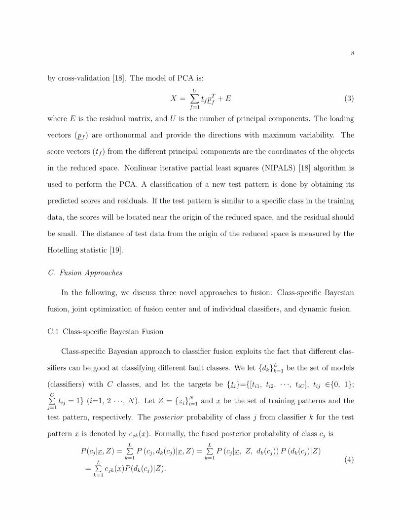
by cross-validation [18]. The model of PCA is:

X =U∑

f=1

tfpTf

+ E (3)

where E is the residual matrix, and U is the number of principal components. The loading

vectors (pf ) are orthonormal and provide the directions with maximum variability. The

score vectors (tf ) from the different principal components are the coordinates of the objects

in the reduced space. Nonlinear iterative partial least squares (NIPALS) [18] algorithm is

used to perform the PCA. A classification of a new test pattern is done by obtaining its

predicted scores and residuals. If the test pattern is similar to a specific class in the training

data, the scores will be located near the origin of the reduced space, and the residual should

be small. The distance of test data from the origin of the reduced space is measured by the

Hotelling statistic [19].

C. Fusion Approaches

In the following, we discuss three novel approaches to fusion: Class-specific Bayesian

fusion, joint optimization of fusion center and of individual classifiers, and dynamic fusion.

C.1 Class-specific Bayesian Fusion

Class-specific Bayesian approach to classifier fusion exploits the fact that different clas-

sifiers can be good at classifying different fault classes. We let {dk}Lk=1 be the set of models

(classifiers) with C classes, and let the targets be {t i}={[ti1, ti2, · · ·, tiC ], tij ∈{0, 1};C∑

j=1tij = 1} (i=1, 2 · · ·, N). Let Z = {zi}N

i=1 and x be the set of training patterns and the

test pattern, respectively. The posterior probability of class j from classifier k for the test

pattern x is denoted by ejk(x ). Formally, the fused posterior probability of class cj is

P (cj|x, Z) =L∑

k=1P (cj, dk(cj)|x, Z) =

L∑k=1

P (cj|x, Z, dk(cj)) P (dk(cj)|Z)

=L∑

k=1ejk(x)P (dk(cj)|Z).

(4)

9

Note that

P (dk(cj)|Z) =P (Z|dk(cj))P (dk(cj))

P (Z)=

P (Z|dk(cj))P (dk(cj))L∑

l=1P (Z|dl(cj))P (dl(cj))

. (5)

We can initialize P (dk(cj))=1/L assuming that all classifiers perform equally on class cj, or

make it proportional to the overall accuracies of classifiers on class cj, i.e.,

P (dk(cj)) =ak(cj)

L∑l=1

al(cj)(6)

where ak(cj) is the accuracy of classifier k on the jth class. Evidently,

ln P (Z|dk(cj)) =N∑

i=1

tij ln ejk(zi). (7)

This simply sums the logs of posterior probabilities for the target class, tij ∈ {0, 1}, over all

the samples corresponding to class cj. Larger this number (closer to zero because the sum is

negative), better is the classifier. So, the numerator of P (dk(cj)|Z) can be evaluated in log

form as:

nkj = ln P (Z|dk(cj)) + ln P (dk(cj)) =N∑

i=1

tij ln ejk(zi) + ln P (dk(cj)). (8)

Then,

P (dk(cj)|Z) =exp(nkj)

L∑l=1

exp(nlj). (9)

Using this, Eq. (4) is used to compute the posterior probability of class cj for a given test

pattern, x.

C.2 Joint Optimization of Fusion Center and of Individual Classifiers

The second approach, motivated by the fact that the decision rules of fusion center

and of individual classifiers are coupled [11], involves the joint optimization of fusion center

10

and of individual classifier decision rules. Given the classifiers, we develop the necessary

conditions for the optimal fusion rule, taking into account costs of decisions. Assume that

there are L classifiers, a fusion center, C fault classes, and the N training targets {t i}. The

decisions of individual classifiers are denoted by {uk}Lk=1while that of fusion center by u0.

The classification rule of kth classifier is uk ∈{1, 2, ..., C} =γk(x ) and that of fusion center

is u0 ∈{1, 2, ..., C}=γ0(u1, u2, ..., uL). The fusion center must decide which one of the

classes has occurred based on the evidence from the L classifiers. The prior probabilities

of each class cj is Pj = Nj/N , where Nj is number of training patterns of class cj. We let

J(u0, cj) be the cost of decision u0 by the committee of classifiers when the true class is cj.

The problem is to find the joint committee strategy γc=(γ0, γ1, γ2, ..., γL) such that the

expected cost E{J(u0, cj)} is a minimum, where E denotes expectation over {x , uk, 0 ≤ k

≤ L} and {cj, 1 ≤ j ≤ C}. The necessary conditions of optimality for the optimal decision

rule is given by [11]:

γ0 : u0 = arg mind0∈{1, 2,···, C}

C∑j=1

{P (u1, u2, · · · , uL|cj) PjJ (d0, cj)} . (10)

The key problem here is to obtain P (u1, u2, ..., uL|cj). For C classes, this would involve

building a table of CL entries, which is clearly intractable in practice. The probability

computation is simplified by correlating each classifier with respect to only the best classifier

from the training data. The best classifier may change during iterations. Formally,

P (u1, u2, · · · , uL|cj) =L∏

k=1P (uk|cj, u1, u2, · · · , uL−1)

≈ P (ubest|cj)L∏

k=1k �=best

P (uk|cj, ubest).(11)

We can estimate P (uk|cj, ubest) by

P (uk = dk|cj, ubest = h) = edkjh (12)

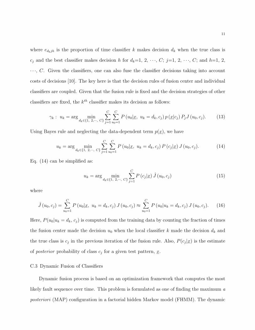
11

where edkjh is the proportion of time classifier k makes decision dk when the true class is

cj and the best classifier makes decision h for dk=1, 2, · · ·, C; j=1, 2, · · ·, C; and h=1, 2,

· · ·, C. Given the classifiers, one can also fuse the classifier decisions taking into account

costs of decisions [10]. The key here is that the decision rules of fusion center and individual

classifiers are coupled. Given that the fusion rule is fixed and the decision strategies of other

classifiers are fixed, the kth classifier makes its decision as follows:

γk : uk = arg mindk∈{1, 2,···, C}

C∑j=1

C∑u0=1

P (u0|x, uk = dk, cj) p (x|cj) PjJ (u0, cj). (13)

Using Bayes rule and neglecting the data-dependent term p(x ), we have

uk = arg mindk∈{1, 2,···, C}

C∑j=1

C∑u0=1

P (u0|x, uk = dk, cj) P (cj|x) J (u0, cj). (14)

Eq. (14) can be simplified as:

uk = arg mindk∈{1, 2,···, C}

C∑j=1

P (cj|x) J (u0, cj) (15)

where

J (u0, cj) =C∑

u0=1

P (u0|x, uk = dk, cj) J (u0, cj) ≈C∑

u0=1

P (u0|uk = dk, cj) J (u0, cj). (16)

Here, P (u0|uk = dk, cj) is computed from the training data by counting the fraction of times

the fusion center made the decision u0 when the local classifier k made the decision dk and

the true class is cj in the previous iteration of the fusion rule. Also, P (cj|x ) is the estimate

of posterior probability of class cj for a given test pattern, x .

C.3 Dynamic Fusion of Classifiers

Dynamic fusion process is based on an optimization framework that computes the most

likely fault sequence over time. This problem is formulated as one of finding the maximum a

posteriori (MAP) configuration in a factorial hidden Markov model (FHMM). The dynamic

12

fusion problem is a specific formulation of the dynamic multiple fault diagnosis (DMFD)

problem [12-14]. In the DMFD problem, the objective is to isolate multiple faults based on

test (classifier) outcomes observed over time. The dynamic fusion problem consists of a set of

possible fault states in a system, and a set of binary classifier outcomes that are observed at

each time (observation, decision) epoch. Evolution of fault states is independent, i.e., there is

no direct coupling among the component states. Each classifier outcome provides information

on a subset of the fault states (the entries with ones in the corresponding column of the

error correcting code (ECC) matrix). Thus, the component states are coupled via classifier

outcomes. At each sample epoch, a subset of classifier outcomes is available. Classifiers are

imperfect in the sense that the outcomes of some of the classifiers could be missing, and

classifiers have missed-detection and false-alarm probabilities associated with them.

Formally, we represent the dynamic fusion problem as DF={S, κ, D, O, ECC, P , A},where S={s1, s2, . . . , sC} is a finite set of C components (failure sources, classes) associated

with the system. The state of a component m is denoted by sm(t) at discrete time epoch t,

where sm(t)=1 if failure source sm is present; sm(t)=0, otherwise. Here κ = {0, 1, . . . , t,. . . ,

T} is the set of discretized observation epochs. The status of all component states at epoch

t is denoted by s(t)={s1(t), s2(t), ..., sC(t)}. We assume that the probability distribution

of initial state is known. The observations at each epoch are subsets of binary outcomes

of classifiers O= {o1, o2, ..., oL}, i.e., on(t) ∈ {pass, fail} = {0, 1}. Let the set of passed

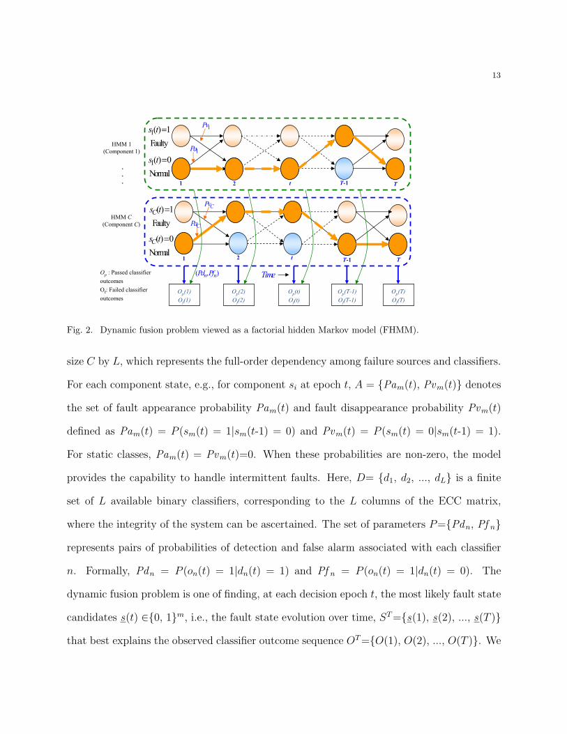
classifier outcomes be Op and that of failed classifiers be Of . Fig. 2 shows the DMFD

problem viewed as a FHMM. The hidden system fault state of mth HMM at discrete time

epoch t is denoted by sm(t). Each fault state sm(t) is modeled as a two-state HMM. Here,

the true states of the component states and of classifiers are hidden.

We also define the ECC matrix ECC = [emn] as the diagnostic matrix (D-matrix) of

13

HMM 1(Component 1)

Op(1)Of(1)

Op(2)Of(2)

Op(t)Of(t)

Op(T-1)Of(T-1)

Op(T)Of(T)

1 2 t T-1 T

( ) 0NormalCs t =

( ) 1FaultyCs t =

Time

1 2 t T-1 T

1( ) 0Normals t =

HMM C(Component C)

1Pa

1Pv

( , )n nPd Pf

1( ) 1Faultys t =

Op : Passed classifier outcomesOf: Failed classifier outcomes

.

.

.

CPv

CPa

Fig. 2. Dynamic fusion problem viewed as a factorial hidden Markov model (FHMM).

size C by L, which represents the full-order dependency among failure sources and classifiers.

For each component state, e.g., for component si at epoch t, A = {Pam(t), Pvm(t)} denotes

the set of fault appearance probability Pam(t) and fault disappearance probability Pvm(t)

defined as Pam(t) = P (sm(t) = 1|sm(t-1) = 0) and Pvm(t) = P (sm(t) = 0|sm(t-1) = 1).

For static classes, Pam(t) = Pvm(t)=0. When these probabilities are non-zero, the model

provides the capability to handle intermittent faults. Here, D= {d1, d2, ..., dL} is a finite

set of L available binary classifiers, corresponding to the L columns of the ECC matrix,

where the integrity of the system can be ascertained. The set of parameters P={Pdn, Pf n}represents pairs of probabilities of detection and false alarm associated with each classifier

n. Formally, Pdn = P (on(t) = 1|dn(t) = 1) and Pf n = P (on(t) = 1|dn(t) = 0). The

dynamic fusion problem is one of finding, at each decision epoch t, the most likely fault state

candidates s(t) ∈{0, 1}m, i.e., the fault state evolution over time, ST ={s(1), s(2), ..., s(T )}that best explains the observed classifier outcome sequence OT ={O(1), O(2), ..., O(T )}. We

14

formulate this as one of finding the maximum a posteriori (MAP) configuration:

ST

= arg maxST

P (ST |OT ). (17)

This problem is computationally intractable. A near optimal polynomial time algorithm

based on Lagrangian relaxation and Viterbi decoding was developed. The details of this

technique, termed a primal-dual optimization framework, may be found in [12-14].

Since the dynamic fusion algorithm is a multiple fault diagnosis algorithm, we may have

both missed classifications as well as spurious faults. We used the following metrics from

[12, 27] to evaluate the performance of the dynamic fusion algorithm.

Missed classification rate (MC): MC is the percentage of faults not inferred by the

algorithm at epoch t. Let s (t) be the inferred states of all failure sources, and s (t) is the

true states. Then MC and average MC over all epochs are obtained as follow:

MC (t) = 1 − |s (t) ∩ s (t)||s (t)| (18)

MC =

T∑t=1

MC (t)

T(19)

False (spurious) classification rate (FC): FC is percentage of fault states which are falsely

inferred by the algorithm as fault states at epoch t. FC and average FC are computed as

FC (t) =|s (t) ∩ ¬s (t)|

C − |s (t)| (20)

FC =

T∑t=1

FC (t)

T(21)

Under single fault assumption, FC can be made zero at the cost of higher MC.

15

III. Simulations

The proposed schemes are evaluated on an engine data set. A realistic automotive engine

model is simulated under various fault conditions in a custom-built ComputeR Aided Multi-

Analysis System (CRAMASR©) [20]. CRAMASR©, a vehicle engine simulator, which is used to

develop vehicular ECUs, is a high-speed, multi-purpose, and expandable system. The engine

system is subject to the following 8 faults: air flow sensor fault (misreading the air flow mass),

leakage in air intake manifold (a hole in the intake tube), blockage of air filter (blocking the

incoming air), throttle angle sensor fault (misreading the throttle angle), air/fuel ratio sensor

fault (misreading the A/F ratio), engine speed sensor fault (misreading the engine speed),

less fuel injection (delivering less fuel from the fuel pump), and added friction (increasing

the friction in cylinders). It also contains the following 5 sensors: air flow meter reading,

air/fuel ratio, vehicle speed, turbine speed, and engine speed. We collected observations of

the 5 sensor readings (measurements) from the CRAMASR© hardware-in-the-loop simulator.

The model was simulated under a steady-state condition, and the operating condition for

the simulation was as follows: 2485 rpm (engine speed), 18◦ (pedal angle), and 86◦ (water

temperature). For each fault class, we performed simulations for 40 different severity levels

(0.5% ∼ 20%); each run is sampled at 2,000 time points with a 0.005-sec sampling interval

(10 seconds of data). The generalized likelihood ratio test(GLRT)-based fault detection tests

[25] for this data set were perfect, i.e., each test had unity probability and zero false alarm

rate. Thus, data consisted of faulty cases only. Consequently, our focus is on fault isolation

only in this paper. We applied our proposed fusion techniques to the data set and compared

them to individual classifier performance measures. Here, 10 randomized data sets of 2-fold

cross-validation were used to assess the classification performance.

16

IV. Results

We implemented and experimented with the three proposed fusion approaches on the

CRAMASR© engine data. Widely used fusion techniques, the majority voting and the naıve

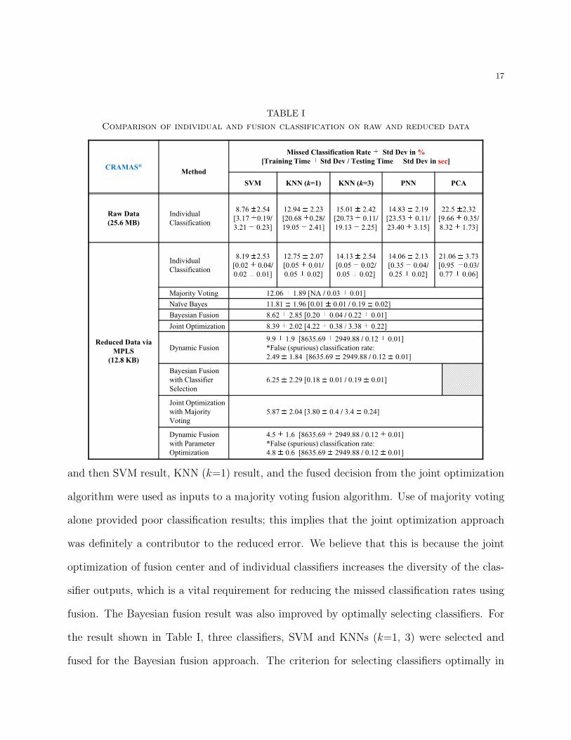
Bayes, were also evaluated and compared with our approaches. The diagnostic results,

measured in terms of missed classification rates and testing times for the 8 faults, are shown

in Table 1. Testing time was computed using MatlabR© software on a 2.3 GHz Intel Pentium

4 processor with 1 GB of RAM. We expect that time shown could be further reduced by a

factor of at least 10 by implementing in the C language. As shown in Table 1, we not only

achieved lower missed classification rates, but also obtained significant data reduction (25.6

MB → 12.8 KB), a factor of 2000. Since data reduction improved classifier performance, the

proposed fusion approaches were mainly evaluated on the reduced data set.

Although majority voting, naıve Bayes, proposed Bayesian fusion and dynamic fusion

(without parameter optimization) approaches for this problem helped marginal classifiers

(PNN, KNNs, and PCA) in reducing the missed classification rates, they were unable to

overcome the best single classifier, SVM. For the CRAMASR© data, SVM algorithm found

for 59 and 44 support vectors for the raw and reduced data, respectively. However, the

proposed Bayesian and dynamic fusion are comparable to the single best classifier, and out-

performed the majority voting and naıve Bayes fusion approaches. Initially the results from

joint optimization approach and class-specific Bayesian fusion were quite similar to that from

the single best classifier (virtually tied statistically to SVM based on McNemar’s test [25]).

However, we were able to reduce the missed classification rates using the joint optimization

approach on marginal classifiers (PNN, KNN (k =3) and PCA) and then applying majority

voting on the fused decision and those from SVM and KNN (k =1). Specifically, the posterior

probabilities from PNN, KNN (k=3), and PCA were fed to the joint optimization algorithm,

17

TABLE IComparison of individual and fusion classification on raw and reduced data

CRAMAS®Method

Missed Classification Rate Std Dev in %[Training Time Std Dev / Testing Time Std Dev in sec]

SVM KNN (k=1) KNN (k=3) PNN PCA

Raw Data(25.6 MB)

IndividualClassification

8.76 2.54[3.17 0.19/3.21 0.23]

12.94 2.23[20.68 0.28/19.05 2.41]

15.01 2.42[20.73 0.11/19.13 2.25]

14.83 2.19[23.53 0.11/23.40 3.15]

22.5 2.32[9.66 0.35/8.32 1.73]

IndividualClassification

8.19 2.53[0.02 0.04/

12.75 2.07[0.05 0.01/

14.13 2.54[0.05 0.02/

14.06 2.13[0.35 0.04/

21.06 3.73[0.95 0.03/Classification 0.02 0.01] 0.05 0.02] 0.05 0.02] 0.25 0.02] 0.77 0.06]

Majority Voting 12.06 1.89 [NA / 0.03 0.01]Naïve Bayes 11.81 1.96 [0.01 0.01 / 0.19 0.02]Bayesian Fusion 8.62 2.85 [0.20 0.04 / 0.22 0.01]Joint Optimization 8.39 2.02 [4.22 0.38 / 3.38 0.22]

9 9 1 9 [8635 69 2949 88 / 0 12 0 01]Reduced Data via MPLS(12.8 KB)

Dynamic Fusion9.9 1.9 [8635.69 2949.88 / 0.12 0.01]*False (spurious) classification rate: 2.49 1.84 [8635.69 2949.88 / 0.12 0.01]

Bayesian Fusion with Classifier Selection

6.25 2.29 [0.18 0.01 / 0.19 0.01]

Joint OptimizationJoint Optimization with Majority Voting

5.87 2.04 [3.80 0.4 / 3.4 0.24]

Dynamic Fusion with Parameter Optimization

4.5 1.6 [8635.69 2949.88 / 0.12 0.01]*False (spurious) classification rate: 4.8 0.6 [8635.69 2949.88 / 0.12 0.01]

and then SVM result, KNN (k=1) result, and the fused decision from the joint optimization

algorithm were used as inputs to a majority voting fusion algorithm. Use of majority voting

alone provided poor classification results; this implies that the joint optimization approach

was definitely a contributor to the reduced error. We believe that this is because the joint

optimization of fusion center and of individual classifiers increases the diversity of the clas-

sifier outputs, which is a vital requirement for reducing the missed classification rates using

fusion. The Bayesian fusion result was also improved by optimally selecting classifiers. For

the result shown in Table I, three classifiers, SVM and KNNs (k=1, 3) were selected and

fused for the Bayesian fusion approach. The criterion for selecting classifiers optimally in

18

class-specific Bayesian fusion and joint optimization was based on both cross-validation and

a coarse optimization. For the dynamic fusion approach, we ran the fusion algorithm with

a sampling interval of 0.5 seconds in order to suppress the noise in the data. Thus, we used

a down sampling rate of 100, and obtained 20 time epochs for the dynamic fusion process.

The results in Table 1 were obtained using 15 SVM classifiers, which are represented by

the columns of the ECC matrix. The ECC matrix was generated using the Hamming code

generation method [21]. The dynamic fusion achieved lower missed classification rate results

as compared to any single classifier results. We experimented with two different approaches

for Pd and Pf in the dynamic fusion process. The first approach used Pd and Pf learned

from the training data of individual classifiers, while a coarse optimization was applied to

learn Pd and Pf, and the optimal parameters were Pd = 0.5∼0.6 and Pf = 0∼0.02 when

they are part of the dynamic fusion. We found that the dynamic fusion approach with pa-

rameter optimization significantly reduces diagnostic error by 45.1% (as compared to SVM,

the single best classifier on the reduced data).

Fig. 3 shows that dynamic fusion with parameter optimization provided the most sig-

nificant improvement and also was the best in classification accuracy. Note that the training

time for the dynamic fusion method depends on how many classifiers (ECC columns) are

used. The more the number of classifiers, the larger is the training time.

Fig. 4 provides a plot of missed classification rate vs. testing time per pattern for all

the approaches considered in this paper, as well as the Pareto efficiency (dashed line) [22].

Pareto efficiency curve indicates all of the potentially optimal approaches to the problem

in that analysts can tradeoff missed classification rate and testing time in an informed way,

rather than considering the full range of fusion approaches. Since our primary focus is on

diagnostic error, the lower values of this measure are preferred to the higher values. The figure

19

e (%

) No Optimization Optimization

8.628.39

9.9

6.25 5.874.5

Cla

ssification

Rate

Mis

sed

C

Fusion Approaches

Joint OptimizationBayesian Fusion Dynamic Fusion

Fig. 3. Comparison of fusion approaches with no parameter optimization and optimization.

18

20

22Individual ClassifiersClassifier Fusion

PCA

)

12

14

16

18

on Error

(%)

Naïve BayesMajority Voting

PNNKNN (k=1)

KNN (k=3)

ficat

ion

Rate

(%)

6

8

10

12

Cla

ssificatio

SVM

Joint Optimization with Majority Voting

Bayesian Fusion with Classifier Selection

Joint OptimizationBayesian Fusion

Dynamic FusionNaïve Bayes

Mis

sed

Cla

ssifi

0 0.5 1 1.5 2 2.5 32

4

6

Testing T ime (sec)

Dynamic Fusion with Parameter Optimization

Bayesian Fusion with Classifier Selection

Testing T ime (sec)

Fig. 4. Comparison of individual and fusion classification on reduced data.

clearly shows that our dynamic fusion with parameter optimization is superior to all other

approaches. However, if one’s focus is on training time or the need for a faster response,

Bayesian fusion with classifier selection would be adequate, while joint optimization with

majority voting would also be a good choice, if the analyst is concerned about training time.

20

V. Conclusions

In this paper, we have proposed and developed three new approaches to classifier fusion.

In addition to individual classifiers, such as the support vector machine (SVM), probabilistic

neural network (PNN), k -nearest neighbor (KNN), and principal component analysis (PCA)

for fault isolation, posterior probabilities from these classifiers were fused by class-specific

Bayesian fusion, joint optimization of fusion center and individual classifiers, and dynamic

fusion. All the approaches were validated on the CRAMASR© engine data (raw and reduced

data sets). Although in terms of missed classification rate, the results of the proposed

approaches before applying optimization were quite close to the single best classifier perfor-

mance, they are generally better than the majority voting and the naıve Bayes-based fusion

approaches. It confirms again that fusing marginal classifiers can increase the diagnostic

performance substantially. We showed that classifier selection in the context of class-specific

Bayesian fusion, majority voting among the best classifiers and fused marginal classifiers,

and parameter optimization in dynamic fusion significantly reduced the overall diagnostic

errors. The key empirical result here is that one needs to learn parameters as part of the

fusion architecture (not standalone) to obtain the best classification performance from a

team of classifiers. This is consistent with the finding in distributed detection theory that

the individual sensors (classifiers in our case) operate at different operating points when part

of a team (fusion in our case) than when they operate alone [23].

Our future research will focus on evaluating the proposed classifier fusion techniques on

various real-world data sets, such as automotive field data, UCI repository, etc. Furthermore,

we plan to explore and compare other fusion techniques that can be applied to fault diagnosis

in automotive systems. For the dynamic fusion research, we also plan to explore relaxation

of the independence assumption and solve the dynamic fusion problem when faults are

21

dependent. Coupled hidden Markov models offer a promising mathematical framework for

the solution of this problem [24]. We also plan to extend the joint optimization approach to

correlated faults via Bayesian network/influence diagram framework.

References

[1] K. Choi, J. Luo, K. R. Pattipati, S. M. Namburu, L. Qiao, and S. Chigusa, “Data

reduction techniques for intelligent fault diagnosis in automotive systems,” Proc. of the

IEEE Autotestcon, Anaheim, CA, September 2006.

[2] P. Nomikos and K. F. MacGregor, “Monitoring batch processes using multiway principal

component analysis,” Amer. Inst. Chem. Eng., vol. 40, no. 8, pp. 1361-1375, 1994.

[3] B. Rasmus, “Multiway calibration. multilinear PLS,” Journal of Chemometrics, vol. 10,

no. 1, pp. 259-266, 1996.

[4] R. O. Duda, P. E. Hart, and D. G. Stork, Pattern Classification, second edition, New

York: Wiley-Interscience, 2001.

[5] C-W. Hsu and C-J. Lin, “A comparison of methods for multi-class support vector ma-

chines,” IEEE Tran. on Neural Networks, vol. 13, no. 2, pp. 415-425, 2002.

[6] Y. Freund and R. E. Schapire, “A decision-theoretic generalization of on-line learning

and an application to boosting,” Journal of Computer and System Sciences, vol. 55, no.1,

pp. 119-139, 1997.

[7] J. Kittler, M. Hatef, R. Duin, and J. Matas “On combining classifiers,” IEEE Tran. on

Patterns Analysis and Machine Intelligence, vol. 20, no. 3, pp. 226-239, March 1998.

[8] L.I.Kuncheva, Combining Pattern Classifiers, John Wiley, 2004.

[9] D. Ruta and B. Gabrys, “An overview of classifier fusion methods,” Computing and

Information Systems, pp. 1-10, 2000.

[10] Y. Bar-Shalom, X. R. Li, and T. Kirubarajan, Estimation with Applications to Tracking

22

and Navigation: Algorithms and Software for Information Extraction, John Wiley and

Sons, 2001.

[11] Z. B. Tang, K. R. Pattipati, and D. L. Kleinman, “A distributed M-ary hypothesis

testing problem with correlated observations,” IEEE Tran. on Automatic Control, vol.

37, no. 7, pp. 1042-1046, July 1992.

[12] S. Singh, K. Choi, A. Kodali, K. R. Pattipati, J. W. Sheppard, S. M. Namburu, S.

Chigusa, D. V. Prokhorov, and L. Qiao, “Dynamic multiple fault diagnosis: mathematical

formulations and solution techniques,” accepted for publication in IEEE Trans. on SMC:

Part A, SMCA07-08-0255, January 2008.

[13] S. Singh, S. Ruan, K. Choi, K. R. Pattipati, P. Willett, S. M. Namburu, S. Chigusa, D.

V. Prokhorov and L. Qiao, “An optimization-based method for dynamic multiple fault

diagnosis problem,” IEEE Aerospace Conference, Big Sky, Montana, March 2007.

[14] S. Singh, K. Choi, A. Kodali, K. R. Pattipati, S. M. Namburu, S. Chigusa, D. V.

Prokhorov, and L. Qiao, “Dynamic fusion of classifiers for fault diagnosis,” IEEE SMC

Conference, Montreal, Canada, October 2007.

[15] I. K. Fodor and C. Kamath, “Dimension reduction techniques and the Classification of

Bent Double Galaxies,” Computational Statistics and Data Analsysis Journal, vol. 41, no.

1, pp. 91-122, November 2002.

[16] C. J. C. Burges, “A tutorial on support vector machines for pattern recognition,” Data

Mining and Knowledge Discovery, vol. 2, pp. 121-167, 1998.

[17] J. K. Shah, Sequential k-NN Pattern Recognition for Usable Speech Classification – A

Revised Report, Speech Processing Lab, Temple Univ., 2004.

[18] S. Wold, P. Geladi, K. Esbensen, and J. Ohman, “Principal component analysis,”

Chemometrics and Intell. Lab. Sys., vol. 2, no. 1-3, pp. 37-52, 1987.

23

[19] P. Nomikos, “Detection and diagnosis of abnormal batch operations based on multi-way

principal component analysis,” ISA Tran., vol. 35, no. 3, pp. 259-266, 1996.

[20] F. Takeshi, Y. Norio, Y. Takeshi, and K. Naoya, “Development of PC-based HIL sim-

ulator CRAMAS 2001,” FUJITSU TEN Technical Journal, vol. 19, no. 1, pp. 12-21,

2001.

[21] R. W. Hamming, “Error detecting and error correcting codes,” Journal of Bell Sys.

Tech., vol 26, no. 2, April 1950.

[22] M. J. Osborne and A. Rubenstein, A Course in Game Theory, MIT Press, 1994.

[23] A. Pete, K. R. Pattipati and D.L. Kleinman, “Optimal team and individual decision

rules in uncertain dichotomous situations,” Public Choice, 75, pp. 205-230, 1993.

[24] L. Xie and Z-Q. Liu, “A coupled HMM approach to video-realistic speech animation,”

Pattern Recognition, vol. 40, no. 8, pp. 2325-2340, August 2007.

[25] K. Choi, M. Azam, J. Luo, S. M. Namburu, and K. R. Pattipati, “Fault diagnosis in

HVAC chillers using data-driven techniques,” IEEE Instrumentation and Measurement

Magazine, vol. 8, no. 3, pp. 24-32, August 2005.

[26] W. Donat, K. Choi, W. An, S. Singh, K. R. Pattipati, “Data visualization, data re-

duction and classifier fusion for intelligent fault detection and diagnosis in gas turbine

engines,” accepted for publication in ASME Journal of Engineering for Gas Turbines and

power, January 2008.

[27] F. Yu, F. Tu, H. Tu, and K. R. Pattipati, “A Lagrangian relaxation algorithm for finding

the MAP configuration in QMR-DT,” IEEE Trans. on SMC: Part A, vol. 37, no. 5, pp.

746-757, September 2007.