TeesRep Teesside Universitys Research Repository httpteesopenrepositorycomtees

This full text version available on TeesRep is the final version of this PhD Thesis

Seetohul L N (2009) Novel applications of optical analytical techniques Unpublished PhD

Thesis Teesside University

This document was downloaded from httpteesopenrepositorycomteeshandle10149117905

All items in TeesRep are protected by copyright with all rights reserved unless otherwise indicated

Novel Applications of Optical

Analytical Techniques

by

Lalitesh Nitin Seetohul

Thesis submitted to the University of Teesside in partial fulfilment of

the requirements for the degree of Doctor of Philosophy

University of Teesside

January 2009

L N Seetohul

ii

AUTHORrsquoS DECLARATION

This thesis is entirely my own work and has at no time been submitted for

another degree

I certify that this statement is correct

L N Seetohul

L N Seetohul

v

Abstract

Novel applications of optical analytical techniques have been demonstrated in

three general areas namely application of broadband cavity enhanced

absorption spectroscopy (BBCEAS) to the detection of liquid phase analytes

the use of total luminescence spectroscopy to discriminate between different

type of teas and the development of an optical sensor to detect ammonia gas

based on the fluorescence quenching of a dye immobilised in a sol gel matrix

A simple BBCEAS setup has been developed with a view to perform

sensitive visible wavelength measurements on liquid phase solutions In the

present work a simple low-cost experimental setup has been demonstrated for

the measurement of the visible spectra of representative liquid-phase analytes

in a 2 mm quartz cuvette placed at normal incidence to the cavity mirrors

Measurements on Ho3+ and sudan black with a white LED and the R ge 099

mirrors covered a broad wavelength range (~250 nm) and represents the

largest wavelength range covered to date in a single BBCEAS experiment The

sensitivity of the technique as determined by the best αmin value was 51 x 10-5

cm-1 and was obtained using the R ge 099 mirrors The best limit of detection

(LOD) for the strong absorber brilliant blue-R was approximately 620 pM

The optical setup was then optimised for the application of BBCEAS

detection to an HPLC system A 1 cm pathlength HPLC cell with a nominal

volume of 70 l was used in this study The cavity was formed by two R ge 099

plano-concave mirrors with a bandwidth of ~ 420 ndash 670 nm Two analytes

rhodamine 6G and rhodamine B were chosen for separation by HPLC as they

were chemically similar species with distinctive visible spectra and would co-

elute in an isocratic separation The lowest value of min obtained was 19 x 10-5

cm-1 The most significant advantage of the HPLC-BBCEAS study over previous

studies arose from the recording of the absorption spectrum over a range of

wavelengths It was demonstrated that the spectral data collected could be

represented as a contour plot which was useful in visualising analytes which

nearly co-eluted The LOD values for the two analytes studied indicated that the

L N Seetohul

vi

developed HPLC-BBCEAS setup was between 54 and 77 times more sensitive

than a commercial HPLC system

For improved sensitivity and lower detection limits the low cost BBCEAS

setup was used with a significantly longer 20 cm pathlength cell where the

mirrors were in direct contact with the liquid phase analyte This also reduced

interface losses The experiments were carried out using both R 099 and R

0999 mirrors The lowest αmin value obtained in this study was 28 x 10-7 cm-1

which is the lowest reported value to date for a liquid phase measurement

making this study the most sensitive liquid phase absorption measurement

reported The lowest LOD recorded was 46 pM and was obtained for

methylene blue with the R 0999 mirrors

A novel application of total luminescence spectroscopy to discriminate

between different types of teas objectively was also investigated A pattern

recognition technique based on principal component analysis (PCA) was

applied to the data collected and resulted in discrimination between both

geographically similar and dissimilar teas This work has shown the potential of

fluorescence spectroscopy to distinguish between seven types of teas from

Africa India Sri Lanka and Japan Geographically similar black teas from 15

different plantation estates in Sri Lanka were also studied The visualisation

technique allowed the separation of all 11 types of teas when the first two

principal components were utilised

The final part of the thesis describes the development of an optical

sensor for the detection of ammonia gas The operation of the sensor depended

on the fluorescence quenching of the dye 9 amino acridine hydrochloride (9

AAH) immobilised in a sol gel matrix It was also shown that the sensor

response was not affected by the presence of acidic gases such as HCl and

SO2 The final version of the sensor made use of dual channel monitoring to

improve the sensitivity of the sensor Measurements using diluted mixtures of

ammonia gas in the range 5 -70 ppm showed that the response of the sensor

was nonlinear with the sensitivity increasing at lower concentrations The

measurement of the baseline noise allowed the LOD to be estimated at ~400

ppb

L N Seetohul

vii

ACKNOWLEDGEMENTS

I would like to express my gratitude to my first supervisor Dr Meez Islam for all

his support patience and constant encouragement throughout my study at the

University of Teesside and also for allowing me to pursue all the ideas I have

had along the way

I am also grateful to my second supervisor Prof Zulfiqur Ali for offering me the

opportunity to be part of his research group for much precious advice and also

for good values and principles he has instilled in me

I would like to acknowledge my third supervisor Dr Steve Connolly

Many thanks to Dr Simon Scott and Dr David James as our numerous

discussions have given me the most interesting insights into various aspects of

research

Thanks to Dr Simon Bateson for his help in development of the miniaturised

ammonia sensor

Thanks to Dr Liam O‟Hare my MSc project supervisor for his support

Furthermore I am thankful to all the staff and technicians involved especially

Helen Hodgson and Doug McLellan for their excellent technical assistance and

co-operation

Thanks to my uncle and aunt for their love affection and continued support

I am indebted to my brothers sister sister in law niece and last but not the

least my parents for all their love encouragement and also for having always

been supportive of my dreams and aspirations Thank you for being such a

wonderful family

NITIN

L N Seetohul

viii

TABLE OF CONTENTS

10 NOVEL APPLICATIONS OF OPTICAL ANALYTICAL TECHNIQUES 1

11 INTRODUCTION 1

12 THESIS OUTLINE 3

13 PUBLICATIONS RELATED TO THIS DISSERTATION 4

14 OTHER PUBLICATIONS 4

15 PRESENTATIONS 4

16 PUBLICATIONS IN PREPARATION 5

17 REFERENCES 5

20 INTRODUCTION TO CAVITY BASED ABSORPTION

SPECTROSCOPY 6

21 INTERACTION OF LIGHT WITH MATTER 6

211 Absorption spectroscopy 9

212 Derivation of the Beer-Lambert law 10

22 COMMON TYPES OF INSTRUMENTS USED FOR ABSORPTION

MEASUREMENTS 12

221 Application of absorption spectroscopy 13

23 CAVITY BASED TECHNIQUES 14

231 Cavity Mirrors 15

232 Types of optical cavities 16

233 Cavity mirrors arrangements 17

234 Mode structures of cavities 18

235 Types of detectors 20

24 THE DEVELOPMENT OF CRDS 22

241 Experimental implementations of CRDS 23

242 Advantages of CRDS 25

243 Disadvantages of CRDS 25

25 BASIC THEORETICAL ASPECTS OF CAVITY RING DOWN SPECTROSCOPY

(CRDS) BASED ON PULSED LASER CAVITY RING DOWN SPECTROSCOPY (PL-

CRDS) 26

26 CAVITY ENHANCED ABSORPTION SPECTROSCOPY 27

L N Seetohul

ix

261 CEAS ndash Theoretical Background 29

262 Sensitivity of CEAS and CRDS 31

27 REFERENCES 32

30 BROADBAND CAVITY ENHANCED ABSORPTION SPECTROSCOPY

(BBCEAS) MEASUREMENTS IN A 2 MM CUVETTE 34

31 OPTICAL SETUP AND MEASUREMENT PROCEDURES 35

311 Light Source 35

312 The Cavity 37

313 Charge-Coupled Device Spectrograph 38

32 EXPERIMENTAL METHODOLOGY 43

33 RESULTS 47

331 Measurement of the dynamic range of the technique 50

34 DISCUSSION 53

341 Comparison with Previous Liquid-Phase Cavity Studies 56

35 CONCLUSION 60

36 REFERENCES 61

40 APPLICATION OF BROADBAND CAVITY ENHANCED ABSORPTION

SPECTROSCOPY (BBCEAS) TO HIGH PERFORMANCE LIQUID

CHROMATOGRAPHY (HPLC) 62

41 EXPERIMENTAL SETUP AND METHODOLOGY FOR HPLC-BBCEAS 68

42 CHOICE OF ANALYTES 71

43 EXPERIMENTAL SETUP AND METHODOLOGY FOR THE COMMERCIAL HPLC

SYSTEM 72

44 RESULTS 73

441 Rhodamine 6G 75

442 Rhodamine B 80

443 Discrimination of co-eluting substances using HPLC-BBCEAS 84

45 DISCUSSION 88

451 Comparison of figures of merit obtained from this study 88

452 Comparison with previous studies 91

46 FURTHER WORK 97

47 CONCLUSION 99

48 REFERENCES 100

L N Seetohul

x

50 LIQUID PHASE BROADBAND CAVITY ENHANCED ABSORPTION

SPECTROSCOPY (BBCEAS) STUDIES IN A 20 CM CELL 101

51 OPTICAL SETUP AND MEASUREMENT PROCEDURES 103

511 Experimental methodology 105

512 Choice of analytes 108

52 RESULTS 109

521 Methylene Blue 110

522 Sudan Black 114

53 DISCUSSION 116

54 CONCLUSIONS 125

55 REFERENCES 126

60 DISCRIMINATION OF TEAS BASED ON TOTAL LUMINESCENCE

AND PATTERN RECOGNITION 127

61 CLASSIFICATION OF TEA 128

62 CONSUMPTION OF TEA 130

621 Quality of tea 130

622 Chemical constituents of tea responsible for taste 131

623 Chemical constituents and biochemistry 132

624 Thermal formation of aroma compounds in tea 135

63 FLUORESCENCE AND TOTAL LUMINESCENCE SPECTROSCOPY 136

631 Principal Components Analysis with TLS 139

64 TOTAL LUMINESCENCE SPECTROSCOPY AND MEASUREMENT PROCEDURES

FOR GEOGRAPHICALLY DIFFERENT TEAS 140

641 Preparation of leaf tea samples for fluorescence analysis (Assam

Kenya and Ceylon) 141

642 Preparation of bottled tea for fluorescence analysis 141

643 Total luminescence analysis 141

644 Statistical analysis 142

65 RESULTS AND DISCUSSIONS 143

66 THE APPLICATION OF TOTAL LUMINESCENCE SPECTROSCOPY TO

DISCRIMINATE BETWEEN GEOGRAPHICALLY SIMILAR TEAS 147

661 Alternative preparation of leaf tea samples for fluorescence

analysis 149

L N Seetohul

xi

662 Total luminescence analysis and statistical analysis 150

67 RESULTS AND DISCUSSIONS 151

68 CONCLUSION 156

69 REFERENCES 157

70 AN OPTICAL AMMONIA SENSOR BASED ON FLUORESCENCE

QUENCHING OF A DYE IMMOBILISED IN A SOL GEL MATRIX 160

71 INTRODUCTION 160

711 The role of ammonia and its detection 164

712 Properties of 9 AAH 169

713 Choice of sol gel matrix 171

714 The sol gel process 171

72 INVESTIGATION OF XEROGEL MATERIALS 173

721 Materials and methodology 174

722 Results and discussions 175

73 MEASUREMENT PROCEDURES FOR THE INITIAL PROTOTYPE 178

731 Materials 178

732 The experimental setup 179

733 Results and discussions 181

734 Effect of acidic gases 183

74 MEASUREMENT PROCEDURES FOR SMALL SCALE PROTOTYPE 185

741 Optimisation of the waveguide sensor 185

742 The dual channel optical sensor 187

743 Discussion and Further Work 192

744 Conclusions 196

75 REFERENCES 197

80 GENERAL CONCLUSIONS 203

81 REFERENCES 206

APPENDIX A 207

L N Seetohul

ix

LIST OF FIGURES

FIGURE 11 ENERGY DIAGRAM SHOWING EXCITATION AND POSSIBLE RELAXATION

MECHANISMS 2

FIGURE 21 ABSORPTION OF RADIATION BY A MOLECULE 8

FIGURE 22 ILLUSTRATION OF THE BEER-LAMBERT LAW 10

FIGURE 23 SCHEMATIC OF THE BASIC COMPONENTS OF A SINGLE BEAM

SPECTROMETER 12

FIGURE 24 SCHEMATIC OF THE BASIC COMPONENTS IN A DOUBLE BEAM

SPECTROMETER 13

FIGURE 25 SCHEMATIC DIAGRAM OF A DIELECTRIC MIRROR COMPOSED OF

ALTERNATING LAYERS OF HIGH AND LOW REFRACTIVE INDEX MATERIALS 15

FIGURE 26 CONFIGURATIONS OF LINEAR OPTICAL CAVITIES 16

FIGURE 27 CAVITY MIRROR ARRANGEMENTS 17

FIGURE 28 CAVITY MODES STRUCTURES 18

FIGURE 29 SCHEMATIC DIAGRAM OF TYPICAL CRDS SETUPS 24

FIGURE 210 SCHEMATIC DIAGRAM OF CEAS EXPERIMENTAL SETUPS 28

FIGURE 211 SCHEMATIC OF BEAM PROPAGATION WITHIN A CEAS SETUP 29

FIGURE 31 WHITE LUXEON bdquoO STAR‟ LED 35

FIGURE 32 RELATIVE INTENSITY VERSUS WAVELENGTH SPECTRA FOR LUXEON LEDS

36

FIGURE 33 LUXEON WHITE LED SPECTRUM 36

FIGURE 34 SCHEMATIC OF AVANTES AVS2000 SPECTROMETER 38

FIGURE 35 A SCHEME OF THE EXPERIMENTAL SETUP FOR LIQUID-PHASE BBCEAS

MEASUREMENTS 39

FIGURE 36 SINGLE PASS ABSORPTION SPECTRA OF BRILLIANT BLUE SUDAN BLACK

COUMARIN 334 AND HO3+ 41

FIGURE 37 ABSORPTION SPECTRUM FOR SUDAN BLACK AND CALCULATED CAVITY

ENHANCEMENT FACTOR 44

FIGURE 38 THE BBCEAS SPECTRA OF 31 X 10-3 M HO

3+ IN WATER 48

FIGURE 39 THE BBCEAS SPECTRA OF 79 X 10-8 M BRILLIANT BLUE-R IN WATER 49

FIGURE 310 THE BBCEAS SPECTRUM OF 40 X 10-6 M SUDAN BLACK IN HEXANE AND

31X 10-3M HO3+

IN WATER IN THE RANGE 420ndash670 NM OBTAINED WITH THE

L N Seetohul

x

WHITE LED AND THE R ge 099 MIRROR SET A SCALED SINGLE-PASS SPECTRUM

OF SUDAN BLACK IS ALSO SHOWN 50

FIGURE 311 BBCEAS SPECTRA OF BRILLIANT BLUE-R FOR A RANGE OF LOW

CONCENTRATIONS FROM ~7 NM TO ~50 NM OBTAINED USING THE RED LED AND

THE R ge 099 MIRROR SET 51

FIGURE 312 AN ABSORBANCE VERSUS CONCENTRATION PLOT OF BRILLIANT BLUE-R

IN THE RANGE ~7 NM TO ~5 microM 52

FIGURE 41 SCHEMATIC OF A TYPICAL HPLC SETUP 62

FIGURE 42 A SCHEME OF THE EXPERIMENTAL SETUP FOR LIQUID-PHASE HPLC-

BBCEAS MEASUREMENTS 68

FIGURE 43 A REPRESENTATIVE CHROMATOGRAM OF RHODAMINE 6G OBTAINED USING

THE HPLC-BBCEAS SETUP THE INSET SHOWS FULL ABSORPTION PROFILES AT

SELECTED TIMES 70

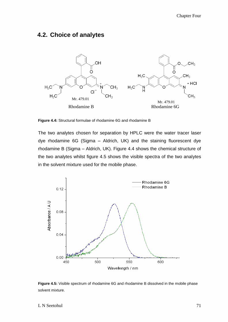
FIGURE 44 STRUCTURAL FORMULAE OF RHODAMINE 6G AND RHODAMINE B 71

FIGURE 45 VISIBLE SPECTRUM OF RHODAMINE 6G AND RHODAMINE B DISSOLVED IN

THE MOBILE PHASE SOLVENT MIXTURE 71

FIGURE 46 PHOTOGRAPH OF THE PERKIN ELMER 200 SERIES INSTRUMENT USED IN

THIS STUDY 72

FIGURE 47 CHROMATOGRAMS OF RHODAMINE 6G MEASURED AT 527 NM 75

FIGURE 48 CHROMATOGRAMS OF RHODAMINE 6G MEASURED AT 527 NM 76

FIGURE 49 AN ABSORBANCE VERSUS CONCENTRATION PLOT FOR RHODAMINE 6G 77

FIGURE 410 AN ABSORBANCE VERSUS CONCENTRATION PLOT FOR RHODAMINE 6G

78

FIGURE 411 AN ABSORBANCE VERSUS CONCENTRATION PLOT FOR RHODAMINE 6G

79

FIGURE 412 AN ABSORBANCE VERSUS CONCENTRATION PLOT FOR RHODAMINE B IN

THE BBCEAS SETUP 80

FIGURE 413 AN ABSORBANCE VERSUS CONCENTRATION PLOT FOR RHODAMINE B 82

FIGURE 414 AN ABSORBANCE VERSUS CONCENTRATION PLOT FOR RHODAMINE B 83

FIGURE 415 A CHROMATOGRAM COMPILED FROM BBCEAS DATA COLLECTED AT 541

NM FOR RHODAMINE 6G AND RHODAMINE B 84

FIGURE 416 A CHROMATOGRAM COMPILED FROM PERKIN ELMER HPLC DATA

COLLECTED AT 541 NM FOR RHODAMINE 6G AND RHODAMINE B 85

L N Seetohul

xi

FIGURE 417 CONTOUR PLOT FOR RHODAMINE B AND RHODAMINE 6G DYE MIXTURE

86

FIGURE 418 CONTOUR PLOT FOR RHODAMINE B AND RHODAMINE 6G DYE MIXTURE

FOR DATA OBTAIN BY THE HPLC- BBCEAS SYSTEM 87

FIGURE 51 A SCHEMATIC OF THE EXPERIMENTAL SETUP FOR LIQUID-PHASE BBCEAS

MEASUREMENTS IN A 20 CM CELL 103

FIGURE 52 SINGLE PASS ABSORPTION SPECTRA OF HEXANE ACETONITRILE

DIETHYLETHER ETHANOL AND WATER RECORDED IN A 10 CM PATHLENGTH CELL

WITH A DOUBLE BEAM SPECTROMETER 106

FIGURE 53 SCALED ABSORPTION SPECTRA OF SUDAN BLACK DISSOLVED IN

ACETONITRILE HEXANE DIETHYLETHER AND ETHANOL RECORDED IN THE 20 CM

CAVITY WITH THE R 099 MIRROR SET 107

FIGURE 54 STRUCTURAL FORMULAE OF SUDAN BLACK AND METHYLENE BLUE 108

FIGURE 55 THE BBCEAS SPECTRUM OF METHYLENE BLUE IN ACETONITRILE IN THE

RANGE 550ndash700 NM 110

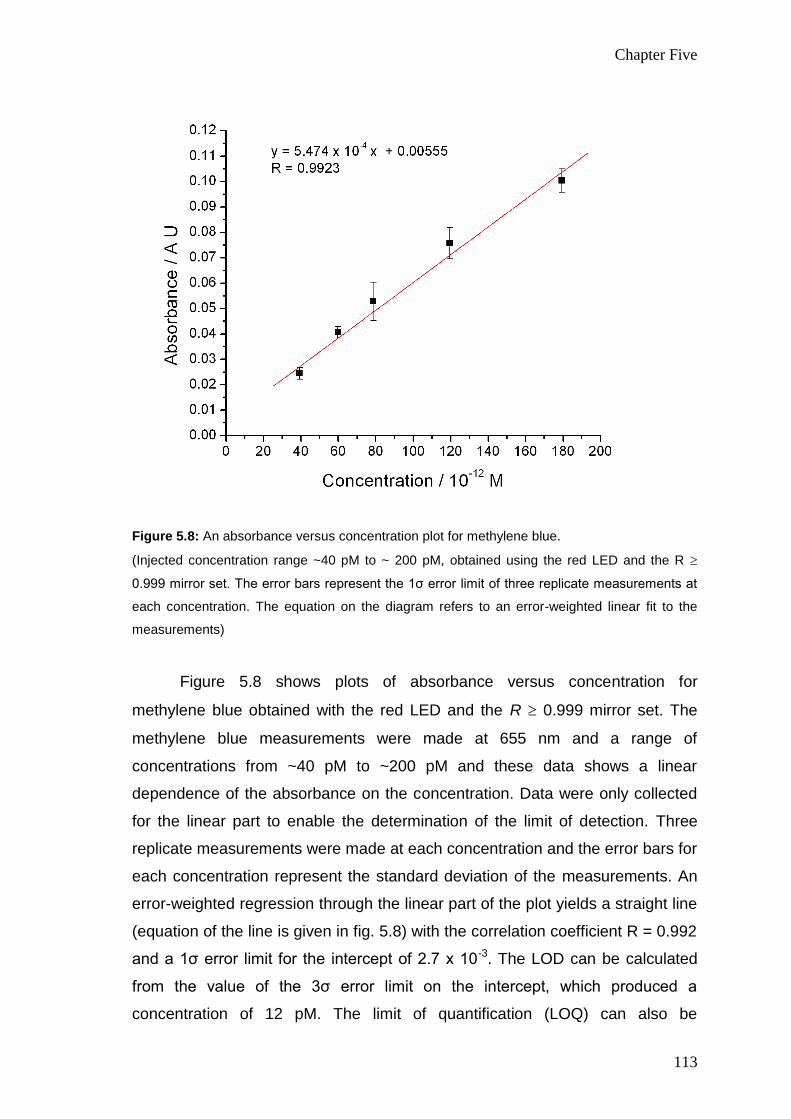
FIGURE 56 AN ABSORBANCE VERSUS CONCENTRATION PLOT FOR METHYLENE BLUE

111

FIGURE 57 THE BBCEAS SPECTRUM OF METHYLENE BLUE IN ACETONITRILE IN THE

RANGE 630ndash660 NM OBTAINED WITH THE RED LED AND THE R ge 0999 MIRROR

SET 112

FIGURE 58 AN ABSORBANCE VERSUS CONCENTRATION PLOT FOR METHYLENE BLUE

113

FIGURE 59 THE BBCEAS SPECTRUM OF SUDAN BLACK IN ACETONITRILE IN THE

RANGE 450ndash700 NM 114

FIGURE 510 AN ABSORBANCE VERSUS CONCENTRATION PLOT FOR SUDAN BLACK 115

FIGURE 61 CLASSIFICATION OF TEA ACCORDING TO THEIR PROCESSING TECHNIQUES

128

FIGURE 62 THE STRUCTURE OF COMMON FLAVANOIDS (CATECHINS) 131

FIGURE 63 STRUCTURE OF HEX-2-ENAL (GREEN FLAVOUR) AND BENZALDEHYDE

(ALMOND FLAVOUR) 134

FIGURE 64 STRUCTURE OF LINALOOL (BITTER FLAVOUR) 134

FIGURE 65 OXIDATIVE DEGRADATION OF CAROTENES DURING TEA FERMENTATION

135

FIGURE 66 A JABLONSKI DIAGRAM 136

L N Seetohul

xii

FIGURE 67 EEM OF BOTTLED BLACK TEA 143

FIGURE 68 EEM OF BOTTLED JAPANESE BLACK TEA WITH THE RESIDUAL EXCITATION

LIGHT REMOVED 143

FIGURE 69 EXCITATION-EMISSION MATRICES OF (A) ASSAM TEA (B) CEYLON TEA (C)

KENYA TEA (D) JAPANESE BLACK TEA (E) JAPANESE GREEN TEA (F) JAPANESE

HOUJI TEA (G) JAPANESE OOLONG TEA 144

FIGURE 610 PCA SCORES PLOT FROM THE TLS OF THE SEVEN VARIETIES OF TEAS

145

FIGURE 611 SOXHLET APPARATUS FOR SOLVENT EXTRACTION 149

FIGURE 612 PCA SCORES LOADING PLOT FOR TOTAL LUMINESCENCE OF SRI LANKAN

BLACK TEAS 151

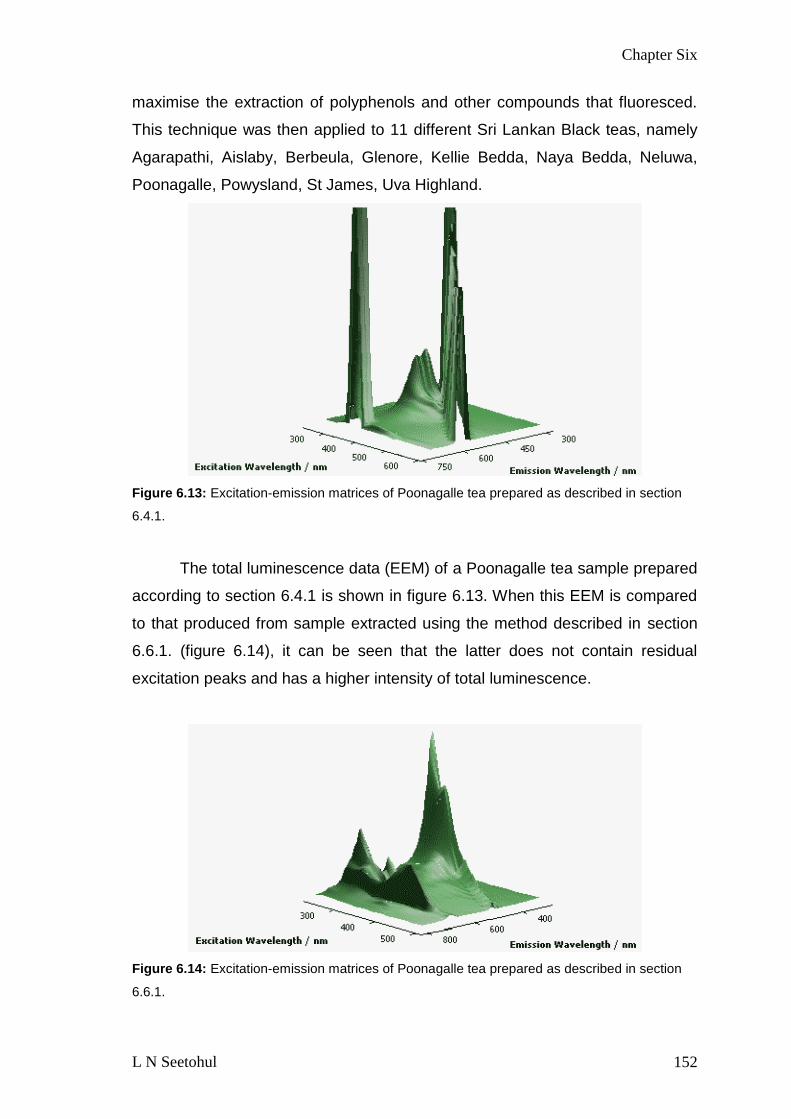
FIGURE 613 EXCITATION-EMISSION MATRICES OF POONAGALLE TEA PREPARED AS

DESCRIBED IN SECTION 641 152

FIGURE 614 EXCITATION-EMISSION MATRICES OF POONAGALLE TEA PREPARED AS

DESCRIBED IN SECTION 661 152

FIGURE 615 PCA SCORES PLOT FOR TOTAL LUMINESCENCE OF SRI LANKAN BLACK

TEAS PREPARED ACCORDING TO SECTION 661 153

FIGURE 616 3D PCA PLOT FOR TOTAL LUMINESCENCE OF SRI LANKAN BLACK TEAS

PREPARED ACCORDING TO SECTION 661 154

FIGURE 71 SCHEMATIC OF DYNAMIC QUENCHING (WHERE F(T) IS THE CONSTANT

EXCITATION FUNCTION Γ IS THE DECAY RATE OF THE FLUOROPHORE IN THE

ABSENCE OF THE QUENCHER KQ IS THE BIMOLECULAR QUENCHING CONSTANT)

161

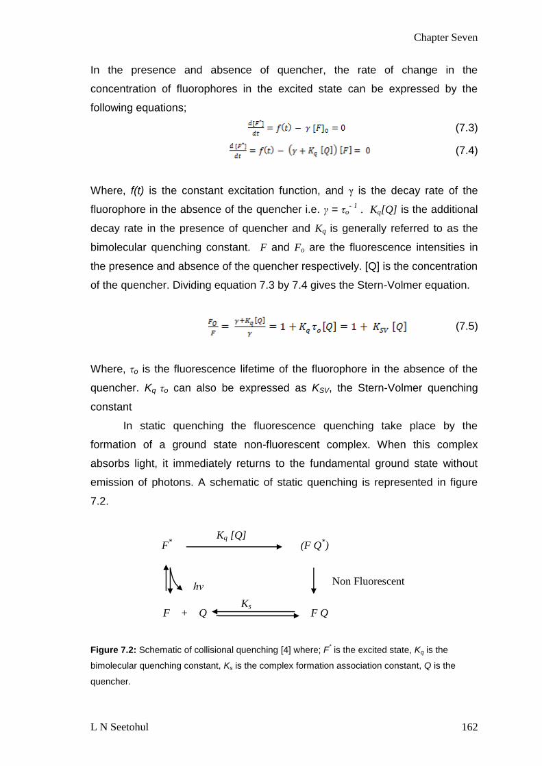
FIGURE 72 SCHEMATIC OF COLLISIONAL QUENCHING [4] WHERE F IS THE EXCITED

STATE KQ IS THE BIMOLECULAR QUENCHING CONSTANT KS IS THE COMPLEX

FORMATION ASSOCIATION CONSTANT Q IS THE QUENCHER 162

FIGURE 73 A SCHEMATIC OF THE NITROGEN CYCLE 165

FIGURE 74 MOLECULAR STRUCTURE OF 9 AAH (C13H10N2 middot HCl) 169

FIGURE 75 FLUORESCENCE SPECTRUM OF 9 AAH IN WATER ETHANOL AND SOL GEL

170

FIGURE 76 SOME OF THE REACTIONS WHICH OCCUR IN THE SOL GEL PROCESS 172

FIGURE 77 SCHEMATIC OUTLINING THE SOL GEL PROCESSING USED IN THIS STUDY

174

FIGURE 78 SEM PICTURES OF REPRESENTATIVE SOL GEL FILMS 176

L N Seetohul

xiii

FIGURE 79 SEM PICTURES OF XEROGEL COATED SLIDE A ndash 50 PTEOS ON

UNCLEANED SLIDE A‟ - 50 PTEOS ON CLEANED SLIDE B ndash 50 MTEOS ON

UNCLEANED SLIDE B‟ - 50 MTEOS ON CLEANED SLIDE C - 50 OTEOS ON

UNCLEANED SLIDE C‟ - 50 OTEOS ON CLEANED SLIDE 177

FIGURE 710 A SCHEMATIC OF THE OPTICAL SENSOR SETUP 179

FIGURE 711 FLUORESCENCE QUENCHING OF THE DYE DOPED SOL GEL ON EXPOSURE

TO CONCENTRATION OF AMMONIA IN THE RANGE 0 ndash 37 times10-6 M (0 ndash 63 PPM) 181

FIGURE 712 A STERN-VOLMER PLOT OF THE FLUORESCENCE QUENCHED DATA 182

FIGURE 713 THE EFFECT OF HIGH CONCENTRATIONS OF (A) HCl AND (B) SO2 ON THE

FLUORESCENCE INTENSITY OF THE SENSOR 184

FIGURE 714 SCHEMATIC OF SETUP TO DETERMINE THE BEST ANGLE FOR THE

DETECTION OF MAXIMUM FLUORESCENCE INTENSITY EXITING THE SUBSTRATE

LAYER 186

FIGURE 715 FLUORESCENCE INTENSITY AT 0O 5O 10O 15O 20O 25O AND 30O 186

FIGURE 716 A SCHEMATIC OF THE DUAL CHANNEL OPTICAL SENSOR 187

FIGURE 717 A BLOCK DIAGRAM OF THE ELECTRONIC DESIGN FOR THE DUAL CHANNEL

SENSOR 188

FIGURE 718 SENSOR RESPONSE WITH 38 PPM AMMONIA 190

FIGURE 719 THE RESPONSE OF THE SENSOR TO AMMONIA GAS IN THE RANGE 5 ndash 70

PPM 190

L N Seetohul

xiii

LIST OF TABLES

TABLE 21 BASIC PARAMETERS OF DIFFERENT DETECTORS 21

TABLE 31 A SUMMARY OF THE RESULTS OBTAINED IN TERMS OF ANALYTE THE LED

USED THE WAVELENGTH OF MEASUREMENT THE REFLECTIVITY OF THE MIRRORS

THE CEF VALUE THE MINIMUM DETECTABLE CHANGE IN ABSORPTION ΑMIN 47

TABLE 32 A COMPARISON BETWEEN THIS STUDY AND PREVIOUS LIQUID-PHASE

CAVITY STUDIES AS A FUNCTION OF TECHNIQUE THE MIRROR REFLECTIVITY BASE

PATHLENGTH THE WAVELENGTH OF MEASUREMENT THE LOWEST VALUE OF αmin

56

TABLE 41 EQUATIONS FOR ISOCRATIC AND GRADIENT ELUTION 64

TABLE 42 A SUMMARY OF THE RESULTS OBTAINED IN TERMS OF ANALYTE USED THE

WAVELENGTH OF MEASUREMENT THE CEF VALUE THE MINIMUM DETECTABLE

CHANGE IN ABSORPTION ΑMIN THE MOLAR EXTINCTION COEFFICIENT Ε AT THE

WAVELENGTH OF MEASUREMENT AND THE LOD OF THE ANALYTE 74

TABLE 43 A COMPARISON BETWEEN THIS STUDY AND PREVIOUS LIQUID-PHASE

CAVITY STUDIES AS A FUNCTION OF TECHNIQUE THE MIRROR REFLECTIVITY BASE

PATHLENGTH THE WAVELENGTH OF MEASUREMENT THE LOWEST VALUE OF αmin

92

TABLE 51 A SUMMARY OF THE RESULTS OBTAINED IN TERMS OF ANALYTE THE

WAVELENGTH OF MEASUREMENT THE REFLECTIVITY OF THE MIRRORS THE CEF

VALUE THE MINIMUM DETECTABLE CHANGE IN ABSORPTION αmin 109

TABLE 52 A COMPARISON BETWEEN THIS STUDY AND PREVIOUS SELECTED LIQUID-

PHASE CAVITY STUDIES 121

TABLE 61 VOLATILE COMPOUNDS CLASSES AND SENSORY CHARACTERISTICS OF

GREEN TEA 133

TABLE 62 ELEVATION AND REGION OF THE SRI LANKAN BLACK TEAS 148

TABLE 71 RATIO OF ALKOXIDE PRECURSORS USED FOR SOL GEL PROCESSING AND

THEIR RESPECTIVE PHYSICAL APPEARANCE 176

TABLE 72 SUMMARY OF CURRENT REQUIREMENTS IN AMMONIA GAS SENSING 193

Chapter One

L N Seetohul 1

Chapter One

10 Novel applications of optical analytical

techniques

11 Introduction

Spectroscopic techniques have the ability to provide sensitive and accurate

determinations of trace and ultratrace species in samples such as

environmental materials high purity solutions biological and medical fluids or

nuclear and radioactive waste substances [1-4] This provides the necessary

information to design experimental probes for trace analysis and discrimination

of complex analytes In most quantitative application of spectroscopic

techniques there is a direct relationship between the analyte concentration and

the luminescence intensity

Spectral data from spectroscopic techniques can also be used for

qualitative analysis and allow characterisation of complex mixtures Often large

amounts of data are generated by spectroscopic techniques and hence there is

a need for effective data analysis to identify trends and relationships in these

data Statistical chemometric techniques can be used as an indirect way to

measure the properties of substances that otherwise would be very difficult to

measure directly [5 6] Multivariate analysis techniques can be applied for

visualisation and pattern recognition One of the most commonly used

visualisation technique is principal component analysis (PCA) [7]

Spectroscopy provides fundamental information about atomic and

molecular properties Much of the current knowledge of the molecular structure

and dynamics of matter is based on the study of the interaction of

electromagnetic radiation with matter through processes such as absorption

emission or scattering Figure 11 is a schematic energy diagram that describes

some of the electronic transitions possible between the ground and excited

state in a molecule (adapted from Wang et al [8])

Chapter One

L N Seetohul 2

Figure 11 Energy diagram showing excitation and possible relaxation mechanisms

During absorption spectroscopy the incident photon (hνA) distorts the

electronic distribution of absorbing molecules and results in energy being

absorbed from the electric field of the photon The experimental determination

of an absorption spectrum requires the measurement of a small change in the

intensity of the incident radiation against a large background and consequently

the sensitivity of the technique in its standard form is poor when compared to

fluorescence measurements Although it should be noted that absorption is an

absolute technique

Fluorescence is a comparatively sensitive technique as measurements

are made against essentially a zero background and consists of three main

stages The first stage being the excitation (absorption) which occurs on the

femtosecond timescale The second stage is the internal conversion (vibrational

relaxation) and the final stage is the loss of excess energy (hνF) on the time

scale of 10-11 ndash 10-7 s [1 9]

Raman spectroscopy is another commonly used spectroscopic technique

and relies on scattering of monochromatic light In Raman scattering the

molecule is excited to a virtual state and relaxes to the ground state with

emission of a photon (hνR) Since vibrational information is specific for the

chemical bonds in molecules the scattered light provides a fingerprint by which

Ground State

hν R

Excited State

Virtual State

Ab

sorp

tio

n

Flu

ore

scen

ce

No

n R

adia

tiv

e

rela

xat

ion

hν F

hν A hν A

Ram

an

Where hν is photon energy and the subscripts A F and R denotes Absorption Fluorescence and Raman scattering respectively

Chapter One

L N Seetohul 3

molecules can be identified Raman scattering is a powerful technique which

provides complimentary information to infrared absorption spectroscopy

12 Thesis outline

The thesis is structured as follows Chapter two provides an introduction to

absorption spectroscopy and its variants with particular emphasis on cavity

based techniques such as cavity ring down spectroscopy (CRDS) and cavity

enhanced absorption spectroscopy (CEAS) Chapter three details a new

implementation of broadband cavity enhanced absorption spectroscopy

(BBCEAS) to perform sensitive visible wavelength measurements on liquid-

phase solutions in a 2 mm cuvette placed at normal incidence to the cavity

mirrors In Chapter four a novel application of BBCEAS to High Performance

Liquid Chromatography (HPLC-BBCEAS) is described and the experimental

results are compared to previous CRDS based studies Chapter five describes

sensitive liquid phase absorption measurements using the low cost BBCEAS

setup from chapter three with a significantly longer 20 cm pathlength cell where

the mirrors were in direct contact with the liquid phase analyte In chapter six a

novel application of total luminescence spectroscopy is used to discriminate

between several types of teas Discrimination of the teas is performed by the

application of multivariate statistical techniques to the spectral data Chapter

seven details the application of a fluorescence based technique for the

detection of ammonia gas A reversible optical sensor based on the

fluorescence quenching of an immobilised fluorophore in a sol gel matrix is

discussed In the final chapter the main results obtained during this PhD

project are summarised

Chapter One

L N Seetohul 4

13 Publications related to this dissertation

SeetohulLN Islam M Ali Z Broadband Cavity Enhanced Absorption

Spectroscopy as a detector for HPLC Analytical Chemistry Volume 81 Issue

10 May 2009 Pages 4106-4112

Islam M Seetohul LN Ali Z Liquid-phase broadband cavity-enhanced

absorption spectroscopy measurements in a 2 mm cuvette Applied

Spectroscopy Volume 61 Issue 6 June 2007 Pages 649-658

Seetohul LN Islam M OHare WT Ali Z Discrimination of teas based on

total luminescence spectroscopy and pattern recognition Journal of the Science

of Food and Agriculture Volume 86 Issue 13 October 2006 Pages 2092-2098

14 Other Publications

Andrew P Henderson Lalitesh N Seetohul Andrew K Dean Paul Russell

Stela Pruneanu and Zulfiqur Ali A Novel Isotherm Modeling Self-Assembled

Monolayer Adsorption and Structural Changes Langmuir Volume 25 Issue 2

January 2009 Pages 639-1264

Novel Optical Detection in Microfluidic Device Z Ali L N Seetohul V Auger M

Islam S M Scott Pub No WO2008065455 International Application No

PCTGB2007050734

15 Presentations

(The name of presenter is underlined)

Liquid phase BBCEAS studies in 20 cm cavity M Islam L Nitin Seetohul and Z

Ali 7th Cavity Ring-Down User Meeting Greifswald Germany (2007)

Fluorescence quenching of dye doped sol gel by ammonia gas L N Seetohul

M Islam and Z Ali University Innovation Centre for Nanotechnology Showcase

Conference UK (2007)

Chapter One

L N Seetohul 5

Broadband liquid phase cavity enhanced absorption spectroscopy Meez Islam

Nitin Seetohul Zulf Ali Cork and UCC 6th Cavity Ring-Down User Meeting

(2006)

16 Publications in preparation

Chapter five Liquid Phase Broadband Cavity Enhanced Absorption

Spectroscopy (BBCEAS) studies in a 20 cm cell (Submitted to Analyst)

Chapter six Total luminescence spectroscopy and measurement procedures

for geographically similar teas

Chapter seven An optical ammonia sensor based on fluorescence quenching

of a dye immobilised in a sol gel matrix

17 References

[1] Schulman G S (Ed) Molecular Luminescence spectroscopy Methods and applications John Wiley amp Sons USA 1985 p 826

[2] Hollas M J (Ed) Modern Spectroscopy Wiley UK 2003 p 480

[3] Becker J S TrAC Trends in Analytical Chemistry 24 (2005) 243

[4] Jose S Luisa B Daniel An Introduction to the Optical Spectroscopy of Inorganic Solids J John Wiley and Sons England 2005 p 304

[5] Miller JN Miller JC An Introduction to the Optical Spectroscopy of Inorganic Solids Pearson education limited UK 2000 p 271

[6] Otto M An Introduction to the Optical Spectroscopy of Inorganic Solids Wiley-VCH Germany 1999 p 314

[7] Gardiner WP Multivariate Analysis Methods in Chemistry (1997) 293

[8] Wang V L Wu H Statistical analysis methods for chemists Wiley-Interscience UK 2007 p 362

[9] Lakowicz J R Principles of Fluorescence Spectroscopy Springer US 2006 p 954

Chapter Two

L N Seetohul 6

Chapter Two

20 Introduction to Cavity Based Absorption Spectroscopy

Spectroscopy provides fundamental information about atomic and molecular

properties A significant fraction of present knowledge on molecular structure

and dynamics of matter is based on the study of the interaction of

electromagnetic radiation with matter through processes such as absorption

emission or scattering One of the most common spectroscopic techniques is

optical absorption which is widely used in chemical and life sciences

Absorption spectroscopy is a simple non-invasive in situ technique which

provides quantitative information about concentration and also absolute

frequency dependent absorption cross section

21 Interaction of light with matter

The nature of light can be described by wave particle duality that is an

electromagnetic wave or a stream of particles (photons) If it is considered as an

oscillating electromagnetic field physical phenomena such as reflection

refraction and diffraction can be understood The Planck equation [1] (equation

21) can be used to show how if light is considered as a stream of photons the

energy of a single photon can be calculated

hch (21)

Where

E = Amount of energy per photon λ = Wavelength of light (nm)

h = Planck‟s constant (663 x 10-34 J s) ν = Frequency of light (Hz)

c = Speed of light (2998 x 108 m s-1)

Chapter Two

L N Seetohul 7

When a beam of light is passed through a medium several effects can

result The simplest possibility would be that the beam emerges in the same

direction with the same intensity This phenomenon is normally described as

transmission Refraction can also occur where the electromagnetic light wave

would have setup transient oscillations in the electrons of the molecules of the

medium and hence slowing down in transit It should be noted that during these

two phenomena no intensity is lost Scattering of light is another observable

phenomenon but one in which some intensity is lost as photons are diverted to

emerge in a direction different to the incident beam A further possibility is that

light can induce some chemical change in the molecules of the medium an

example would be the photoelectric effect where when enough energy is

provided an electron may be expelled completely from a molecule resulting in a

highly reactive free radical [2 3]

The final possibility is that of absorption of light by molecules If the

wavelength of the incident light is such that the energy per photon precisely

matches the energy required for example to excite an electronic transition

these photons do not emerge and are absorbed in the medium [4] Measuring

the absorption of electromagnetic radiation as a function of wavelength allows

the determination of the different types of energy levels present within atomic or

molecular species

The absorption of UV or visible radiation usually corresponds to the

excitation of the outer electrons in atomic or molecular species There are three

types of electronic transition which can typically be considered

(i) Transitions involving π σ and n electrons (mostly exhibited by large organic

molecules)

(ii) Transitions involving charge-transfer electrons (mostly exhibited by inorganic

species called charged transfer complexes)

(iii) Transitions involving d and f electrons (exhibited by atomic species or

compounds containing the transition metals and the lanthanides and actinides)

Chapter Two

L N Seetohul 8

Excited State (π)

Ground State (π)

Excitation corresponding to the absorption of one quantum of energy

A simple molecular electronic transition involving a bonding to anti-

bonding transition ( ) is illustrated in figure 21

Figure 21 Absorption of radiation by a molecule

Most absorption spectroscopy of organic compounds is based on

transitions of n (non-bonding) or π electrons to the π excited state This is

because the absorption peaks for these transitions fall in an experimentally

convenient region of the spectrum (200 - 700 nm) This variation in absorption

with wavelength makes the phenomenon of light absorption a valuable tool for

qualitative and quantitative analysis of chemical and biological molecules [5]

Chapter Two

L N Seetohul 9

211 Absorption spectroscopy

Absorption spectroscopy is considered a universal technique as all species will

display an absorption spectrum at some given wavelength in the

electromagnetic spectrum The strength of absorption is found to depend on a

number of factors namely (i) the pathlength (l) (ii) the concentration (c) of

absorbing molecules and a constant of proportionality which depends on the

identity of the species

Mathematically the phenomenon of absorption can be represented by the

Beer-Lambert Law (commonly known as the Beer‟s Law)

ccI

IAabsorbance

32log 0

10 (22)

Where I = transmitted intensity of light at distance in cm and 0I the

respective incident initial value (when = 0) is the bdquodecay constant‟ which is

dependent on the type of species present The composite proportionality

constant 32 can be replaced by the symbol ε (molar absorbtivity at the

wavelength and it has dimensions M-1 cm-1) which is a property of the

absorbing species c is the molar concentration From equation 22 we can

directly observe that absorbance is linearly related to concentration Hence

absorbance is widely used in life sciences to measure concentration of species

In biology and biochemistry the absorbance of a solution when = 1 cm is

commonly coined by the term optical density (OD) of the solution

Chapter Two

L N Seetohul 10

212 Derivation of the Beer-Lambert law

Figure 22 Illustration of the Beer-Lambert law

The Beer-Lambert law can be derived from the fractional amount of light

absorbed (light transmitted) which is related to the thickness and concentration

of a sample The solution can be regarded as a multilayered arrangement Each

layer is equally populated by light absorbing solute molecules [6]

The change in intensity dI can be expressed as

dLIkdI (23)

Where kλ is the wavelength dependent proportionality constant As L increases I

become smaller hence a negative sign is required

Rearranging equation 23

dLkI

dI (24)

Integrating this equation between limit I to Io and for L between 0 and L gives

LI

IdLk

I

dI

o 0

LkI

I

o

ln (25)

Pathlength of liquid L

I1 ndash dI

dL

Io I1

I

Where Io =Intensity of incident light I1 is the intensity entering the infinitesimal layer dI = Intensity of light absorbed by the layer I = Intensity of a parallel beam of monochromatic light of wavelength λ

passing though the layer dL

Chapter Two

L N Seetohul 11

Since 2303 log10 (x) = ln(x)

Then

3032log 10

Lk

I

Io (26)

Assuming the concentration C is an independent variable we can write

dCIkdI (27)

Integrating equation 8 between limit Io to I and for C between 0 and C gives

CI

IdCk

I

dIo

0

3032log

10

Ck

I

I o (28)

The equations 6 and 8 can be combined for both L and C to give

3032log

10

LCk

I

I o (29)

I

I o

10log is the absorbance (A) 3032

k

is the molar absorbtivity (ε) when the

concentration (C) is given in g mol dm-3

The equation can be expressed as

A = εCL (210)

Chapter Two

L N Seetohul 12

22 Common types of instruments used for absorption

measurements

Figure 23 highlights the basic components of a single beam

spectrophotometer Single beam spectrometers are widely used in routine

laboratory measurements over a range of wavelength most commonly in the

UV-visible range

Figure 23 Schematic of the basic components of a single beam spectrometer

Light emitted by the light source typically an incandescent lamp passes

through a monochromator which can be scanned to select a particular

wavelength and then through the sample cuvette and onto the detector

(typically a photomultiplier tube or photodiode) The intensity reaching the

detector in presence and absence of the sample is used to calculate the

absorbance of the sample at a particular wavelength The monochromator is

then scanned through a range of wavelengths to obtain the absorption spectrum

of the sample The sensitivity of the instrument is limited by fluctuations in the

intensity of the light source which manifests itself as noise on the absorption

spectrum Additional sources of noise arise from the detector and associated

electronic components [4]

Light

source Monochromator Cuvette Detector

Chapter Two

L N Seetohul 13

Figure 24 Schematic of the basic components in a double beam spectrometer

A convenient way to reduce instrumental noise from fluctuations in the

intensity of the light source is to use a double beam spectrometer Figure 24

shows a schematic of a double beam spectrometer (also known as a split beam

spectrometer) the monochromated light is split into two where one beam

passes through the sample and the other through the reference cell The

difference in intensity between the reference and sample beam therefore

represent the light absorbed by the sample [4] The double beam configuration

offers several advantages over single beam spectrometers In the double beam

configuration fluctuations in the intensity of the light source are removed from

the absorption spectrum Hence better sensitivity is achieved

221 Application of absorption spectroscopy

Direct absorption spectroscopy of atoms and molecules in the gas phase yields

both absolute quantitative concentrations as well as absolute frequency-

dependent cross-sections and is a very powerful tool in analytical and physical

chemistry [3 7] Sensitive absorption spectroscopy techniques are commonly

applied as diagnostic techniques In a conventional absorption experiment one

measures the amount of light that is transmitted through a sample A drawback

of conventional absorption spectroscopy is that its sensitivity is limited

compared to spectroscopic techniques which are based on the detection of

phenomena induced by absorption of light such as pressure changes in

photoacoustic spectroscopy fluorescence in laser induced fluorescence (LIF)

or ion production in resonant enhanced multiphoton ionization (REMPI) The

main reason is that these techniques are background free whereas in direct

absorption a small attenuation in transmitted light has to be measured on top of

Sample cuvette Monochromator Detector

Reference cuvette

Light

source

Chapter Two

L N Seetohul 14

a large background A disadvantage is that these techniques do not provide an

absolute measure of the concentration of a given analyte and must be first

calibrated Often the calibration process is complex and time consuming

Several methods exist for increasing the sensitivity of absorption

spectroscopy These include frequency and wavelength modulation schemes

that have been discussed in several reviews [8-11] and will not be discussed

further here and also by increasing the absorption pathlength though cavity

based techniques

23 Cavity based techniques

The biggest advances in improving the sensitivity of absorption measurements

have occurred over the last 20 years [9 12] as a result of the application of

cavity based techniques These have utilised optical cavities formed from two

high reflectivity dielectric mirrors (R gt 099) to increase the effective pathlength

of measurement and have resulted in two general techniques namely cavity

ring down spectroscopy (CRDS) and cavity enhanced absorption spectroscopy

(CEAS) The following sections firstly describe some of the methodology

common to both techniques and then a consideration of the important

characteristics of each technique in turn

Chapter Two

L N Seetohul 15

231 Cavity Mirrors

Figure 25 Schematic diagram of a dielectric mirror composed of alternating layers of high and

low refractive index materials

Dielectric mirrors are preferred over metallic mirrors for use in cavities as they

can be constructed to have much higher reflectivities also the transmission

through dielectric mirrors can be made close to (1-R) even for high reflectivities

and multiple layer depositions For metallic mirrors the transmission through the

mirrors falls off to zero for deposition thicknesses beyond a few hundred

nanometres Figure 25 as expressed by Busch et al [8] shows a schematic

diagram of the cross-section of a multilayer dielectric mirror These mirrors are

wavelength selective and high reflectivity is obtained over a selected range of

wavelengths or frequencies by constructive interference of the waves reflected

at each discontinuity in refractive index Each layer is made a quarter of a

wavelength thick and of a suitable material so as to make all the reflected

waves in phase Hence the dielectric mirrors function on the basis of

constructive interference of light reflected from the different layers of the

dielectric stack Typical high reflectance mirrors may have up to forty quarter-

wavelength dielectric layers that alternate between a high and low refractive

index coatings Common dielectric materials used to fabricate the layers that

make up the reflecting sandwich of these mirrors include silicon dioxide (SiO2)

titanium dioxide (TiO2) zirconia (ZrO2) and thorium fluoride (ThF4) [9] The

multilayer dielectric mirrors have characteristics such as resistance to abrasion

High refractive

index material Low refractive

index material frac14 wave optical path

Chapter Two

L N Seetohul 16

and resistance to chemical attack that makes them ideal for cavity based

spectroscopy State of the art dielectric mirrors can be fabricated to have ultra-

high reflectivities of R ge 099999 over a narrow range of wavelengths (typically

~50 nm in the visible part of the spectrum) by depositing several hundred

dielectric layers [9] Alternatively they can be fabricated to have moderately

high reflectivity (R 0995) but over a much wider wavelength range eg the

entire visible spectrum (400 ndash 700 nm) This is achieved by depositing multiple

dielectric stacks with slightly different central wavelength One practical

consequence is that the variation of the reflectivity profile with wavelength is no

longer smooth as is the case for single wavelength dielectric stacks and instead

contains bdquospikes‟ in the profile where the reflectivity abruptly changes

232 Types of optical cavities

Optical cavities can be produced by arranging at least two mirrors facing each

other and placed at some distance from each other so that light is reflected

back and forth between the mirrors The three possible optical arrangements

that produce linear cavities are shown in figure 26

Figure 26 Configurations of linear optical cavities

Optical cavities can be classified into two categories stable or unstable

according to their losses A cavity is geometrically stable if a paraxial ray bundle

is refocused within the cavity after successive reflection off the mirrors so that

the optical energy is trapped within the cavity On the other hand if the optical

energy escapes the cavity after several reflections then it is said to have an

unstable geometry A stable cavity can be achieved when at least one of the

cavity mirrors is concave

(a) plano-plano (b) plano-concave (c) plano-concave

Chapter Two

L N Seetohul 17

R1= R2 = L (Confocal)

R1= R2 = L2 (Concentric)

R1= R2 gt L (Long-radius)

233 Cavity mirrors arrangements

By varying the distance between a pair of concave mirrors different types of

cavities can be produced Figure 27 shows some of the configurations that can

be achieved

Figure 27 Cavity mirror arrangements

The cavities show different properties in terms of spot size and sensitivity

with regard to misalignment For application in cavity based experiments the

preferred configuration is one which shows insensitivity towards misalignment

whilst the optimum spot size generally depends on the application When R1 =

R2 = L2 the cavity is referred to as a concentric cavity When R1 = R2 = L the

focal points of both mirrors coincides halfway between mirror separation and it

is referred to as a confocal cavity A confocal cavity is relatively insensitive to

misalignment but produces a rather small spot size A long-radius cavity

(variation of a Fabry-Perot cavity) is produced when R1 = R2 gt L This cavity

produces a large spot size but requires careful alignment procedures to

achieve a stable cavity For any given experimental setup the wavelength

range that can be covered depends on the reflectivity characteristics of the

mirrors used in the cavity [9 13]

Chapter Two

L N Seetohul 18

234 Mode structures of cavities

Interference occurs between pulse fragments propagating in the same direction

inside the cavity for laser pulses whose length exceeds the round-trip length of

a cavity These interference effects can be explained by the FabryndashPerot theory

of resonators [14] The FabryndashPerot resonant cavity is essentially a pair of

highly reflective mirrors When a monochromatic laser source is incident on the

cavity such that the distance between the two mirrors is an integer multiple of

the laser wavelength the light experiences constructive interference as it

bounces back and forth inside the cavity Under such conditions the light

intensity builds inside the cavity to an equilibrium value and a small portion of

the signal escapes through each mirror Therefore the interference pattern

formed in a cavity shows resonance enhancement of intensity for the

frequencies interfering bdquobdquoin phase‟‟ and quenching of intensity for the

frequencies interfering bdquobdquoout of phase‟‟ [15]

0

002

004

006

008

01

012

014

0 5 10 15 20

Frequency

Tra

nsm

itta

nce

Light Source

Resonant

cavity modesΔν

Figure 28 Cavity modes structures

The cavity modes are shown in figure 28 and the frequency interval

between two modes the free spectral range (FSR) can be expressed as [15]

L

c

2 (211)

Where c = speed of light L is the cavity length

Chapter Two

L N Seetohul 19

It is this interference pattern that is the source of etalon effects that

cause variation of the intensity of light transmitted through a cavity as a function

of frequency The optical frequencies for which the intensity of light inside the

cavity is resonantly enhanced give rise to the longitudinal modes of the cavity

[13 14 16] The gap between resonant frequencies of the Fabry-Perot etalon is

the Free Spectral Range (FSR) and it can be described by the following

equation [15]

nL

cFSR

2 (212)

Where c ndash is the speed of light n ndash is the refractive index of the medium and L

ndash is the length of the cavity

The mode structure of optical cavities introduces experimental

consequences for CRDS and CEAS setups where the linewidth of the laser

source is less or comparable to the FSR of the cavity For these setups the

transmission of the cavity can be zero unless the laser wavelength is in

resonance with the cavity modes and consequently it is common practice to

rapidly change the length of the cavity by placing one of the cavity mirrors on a

piezoelectric transducer (PZT) This allows the laser wavelength to be partly in

resonance with one or more of the cavity modes during the timescale of the

experiment For setups using broadband light sources such as BBCEAS the

mode structure of the cavity is normally not an issue as several thousand cavity

modes will typically be accessible by the light source ensuring substantial

transmission through the cavity

Chapter Two

L N Seetohul 20

235 Types of detectors

Despite the large number of detectors available they can be classified under

two major groups namely thermal and photoelectric (quantum) detectors The

thermal detectors respond to heat energy gained by the absorption of photons

The intensity of the incident light can therefore be determined by monitoring a

temperature dependent physical magnitude of the material (ie change in

electrical resistance) As thermal detectors depends on the total amount of heat

energy reaching the detector their response is independent of wavelength [4

5] Since the detector is based on heating a thermocouple the time response is

slow One advantage of these detectors is the flat response towards incoming

radiation Examples of common thermal detectors used in spectroscopy are

thermopiles and pyroelectric detectors [3]

In photoelectric detectors a change in physical magnitude occurs when

quanta of light energy interact with electrons in the detector material generating

free electrons Therefore theoretically single photons could be detected When

light of an adequate wavelength reaches a photoelectric detector and is

absorbed the carrier density changes causing a change in electrical

conductivity of the semiconductor The change in conductivity is proportional to

the intensity of incident light The main limitation of this kind of detector is the

noise caused by thermal excitation If there is a large current generated by the

detector in the absence of incident light (dark currentnoise) the sensitivity of

the photoelectric detector becomes poor Hence they are sometimes cooled

during operation in order to reduce the dark currentnoise Commonly used

photoelectric detectors include photoconduction detectors photodiodes and

photomultipliers Even in the absence of incident light these detectors

generate output signals that are usually randomly distributed in intensity and

time and these signals are due to noise The two main type of noise in

photoelectric detectors are dark noise which has been described above and

shot noise

Shot noise is the inherent noise in counting a finite number of photons

per unit time Photons reaching the detector are statistically independent and

uncorrelated events Although the mean number of photons arriving per unit

Chapter Two

L N Seetohul 21

time is constant on average at each measured time interval the number of

detected photons may vary The major source of shot noise in semiconductors

is due to the random variations in the rate at which charge carriers are

generated and recombine [5] Table 21 describes basic parameters such as the

spectral range and time constant of different types of detectors [17]

Table 21 Basic parameters of different detectors

Detector Spectral range (nm) Time constant

Thermopile 100 ndash 4000 20 ms

Pyroelectric 100 ndash 4000 10 ns ndash 100 ps

Photomultiplier 100 ndash 1500 05 ndash 5 ns

Photodiodes 200 ndash 4000 10 ndash 100 ns

Avalanche photodiodes 200 ndash 1000 10ps ndash 1 ns

Photoconduction 1000 ndash 20000 ~ μs

The thermal detectors have a large spectral range from ultraviolet to mid-

infrared region of the electromagnetic spectrum and the pyroelectric detectors

shows faster time constant compared to thermopile detectors Photoelectric

detectors mainly have a working range from the UV region of the

electromagnetic spectrum to the mid infrared The working range of

photomultipliers span from the ultraviolet to the near-infrared The intensity of

light involved in cavity enhanced spectroscopy tends to be very low Under

these conditions the noise produced by the detector can be greater than the

detected signal The simplest method to minimise the level of noise is through

signal averaging by performing consecutive measurements and then calculating

the average signal If the source of noise is randomly distributed in time then

the signal to noise ratio (SN) should improve by radicn (where n is the number of

measurements)

Chapter Two

L N Seetohul 22

24 The development of CRDS

Herbelin et al [18] were the first to propose the use of an optical cavity for

measuring the reflectance of mirror coatings The reflection losses are in a way

the absorption of the optical cavity The reflectance of their mirrors was

accurately determined by modulating the intensity of a continuous wave (CW)

light beam and measuring the phase shift introduced by the optical cavity The

phase shift was inversely related to the sum of the reflected losses in the cavity

There were major limitations to the precision of their technique due to the noisy

character of the transmitted laser intensity

Anderson et al [19] in 1984 unaware of previous work carried out by

Kastler [14] demonstrated that the high reflectance of mirrors could be

measured with higher accuracy by suddenly switching off the CW light source

when the intracavity field exceeded a certain threshold value and recording the

subsequent intensity decay of the light in the optical cavity

O‟Keefe and Deacon [20] in 1988 showed that the problems associated

with mode coincidences could be bypassed by using a pulsed laser and

achieved sensitivity greater than that attained by using stabilised continuous

wave light sources Furthermore they were the first to propose that a simple

experimental design for measuring cavity losses could be achieved as no

electronics were needed for monitoring the intracavity power or switching off the

laser before observing the decay transient They also demonstrated the

sensitivity by measuring the Cavity Ring Down (CRD) absorption spectrum of

the weak bands of molecular oxygen They reported the first minimum

detectable loss which was 2 x 10-8 cm-1 for a cavity of 25 cm with cavity mirrors

of R ge 09999 [20] Their study is generally acknowledged as the first

experimental demonstration of CRDS

Chapter Two

L N Seetohul 23

241 Experimental implementations of CRDS

CRDS is a sensitive absorption technique in which the rate of absorption rather

than the magnitude of the absorption of a light pulse confined in an optical

cavity are measured [21] A schematic of the experimental setup of a

conventional CRDS system is shown in figure 8 (a) Typically a tuneable pulsed

laser having pulse duration of ~ 15 ns is used as the light source [10] The

radiation from the laser is introduced into the cavity with the appropriate mode-

matching optics required as there is a need to match the field distribution of the

incident laser source to that of the recipient cavity mode CRDS cavities

generally consist of two identical plano-concave high reflectivity mirrors (R ge

0999) with radius of curvature between 25 cm and 1 m separated by a distance

such that the cavity is optically stable [10] The sample is placed inside the high-

finesse optical cavity consisting of the two mirrors The short laser pulse that is

coupled into the cavity is reflected back and forth inside the cavity and every

time the light pulse is reflected off one of the mirrors a small fraction of the light

leaks out of the cavity Instead of measuring the total intensity of light exiting the

cavity one determines the decay time by measuring the time dependence of

the light leaking out of the cavity Hence the rate of absorption can be

obtained the more the sample absorbs the shorter is the measured decay time

[9]

Laser

Resonant Cavity

Cavity Mirrors

Detector

AD Converter

Pulsed Cavity

Ring Down

(CRD) Setup

(a)

Chapter Two

L N Seetohul 24

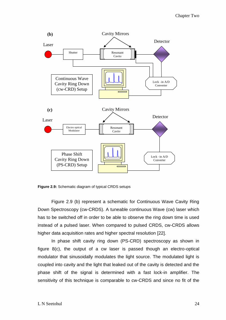
Figure 29 Schematic diagram of typical CRDS setups

Figure 29 (b) represent a schematic for Continuous Wave Cavity Ring

Down Spectroscopy (cw-CRDS) A tuneable continuous Wave (cw) laser which

has to be switched off in order to be able to observe the ring down time is used

instead of a pulsed laser When compared to pulsed CRDS cw-CRDS allows

higher data acquisition rates and higher spectral resolution [22]

In phase shift cavity ring down (PS-CRD) spectroscopy as shown in

figure 8(c) the output of a cw laser is passed though an electro-optical

modulator that sinusoidally modulates the light source The modulated light is

coupled into cavity and the light that leaked out of the cavity is detected and the

phase shift of the signal is determined with a fast lock-in amplifier The

sensitivity of this technique is comparable to cw-CRDS and since no fit of the

Laser

Resonant Cavity

Cavity Mirrors

Detector

Lock ndashin AD Converter

Electro optical

Modulator

Phase Shift

Cavity Ring Down

(PS-CRD) Setup

(c)

Laser

Resonant Cavity

Cavity Mirrors

Detector

Shutter

Lock ndashin AD

Converter

Continuous Wave

Cavity Ring Down

(cw-CRD) Setup

(b)

Chapter Two

L N Seetohul 25

ring down transient is required PS-CRDS can easily be performed with

analogue detection electronics [8 11 18 20 23]

242 Advantages of CRDS

Since the absorption is determined from the time dependent behaviour of the

signal it is independent of pulse to pulse fluctuations of the laser The effective

absorption pathlength which depends on the reflectivity of the cavity mirrors

can be very long (up to several kilometres) while the sample volume can be

kept rather small The main advantage of CRDS is that the absorption

coefficient can be calculated directly from the measured ringdown time constant

and thus the concentration of species can be determined absolutely if the

absorption cross section is known [10]

243 Disadvantages of CRDS

Cavity ring down spectroscopy cannot be applied effectively to liquids The

large scattering losses in liquids coupled with short cavity lengths results in a

very short ring down time that is difficult to accurately measure Most liquid

cells especially those used in HPLC and CE have pathlengths on the order of

1 ndash 10 mm Even with high reflectivity mirrors the ringdown time of these cells

is less than 100 nanoseconds which require highly specialised experimental

setups with short pulsewidth (lt 1 ns) light sources and fast response detection

systems with instrumental response times of less than 1 ns [11 24] CRDS is

an order of magnitude more expensive than some alternative spectroscopic

techniques due to the experimental complexity requirement for laser systems

fast detection system and high reflectivity mirrors

Chapter Two

L N Seetohul 26

25 Basic theoretical aspects of Cavity Ring Down

Spectroscopy (CRDS) based on Pulsed Laser

Cavity Ring Down Spectroscopy (PL-CRDS)

In a typical CRDS experiment a light pulse with a spectral intensity distribution

I(v) and a duration which is shorter than the CRD time τ is coupled into a non-

confocal optical cavity consisting of two highly reflecting mirrors The fraction of

the light that is successfully coupled into the cavity bounces back and forth

between the mirrors The intensity of the light inside the cavity decays as a

function of time since at each reflection off a mirror a small fraction of the light

is coupled out of the cavity The time dependence of the intensity inside the

cavity is easily monitored by measuring the intensity of the light exiting the

cavity In an empty cavity this ring down time is a single-exponentially decaying

function of time with a 1e CRD time τ which is solely determined by the

reflectivity R of the mirrors and the optical pathlength d between the mirrors

The presence of absorbing species in the cavity gives an additional loss

channel for the light cavity and will still decay exponentially resulting in a

decrease in the CRD time τ The intensity of light exiting the cavity is given by

[11]

tc

d

RdItI o

lnexp)(

(213)

Where the reciprocal ring-down time (decay time for non exponential decay) is

given by

d

cRcCRD ln

1

(214)

The absorption coefficient α can be represented by

cavityemptycavityfilledc

CRDCRD

111 (215)

Chapter Two

L N Seetohul 27

26 Cavity enhanced absorption spectroscopy

The quantitative measurement of absorbing species using cw-CRDS

measurements can be carried out without the performing independent

calibration and offers great sensitivity Nevertheless such performance is not

always required from a sensitive absorption technique[11] The complexity and

cost of cw-CRDS experiments can be high especially in systems where a high

speed data acquisition scheme is required The weak signals leaking out of the

cavity is captured by fast response expensive detectors then amplified and

digitised without degradation of the time resolution in order to be able to fit the

low noise ring down decays In order to simplify CRDS Cavity enhanced

absorption spectroscopy (CEAS) was developed to eliminate the constraint of

digitalisation of the low noise ring down decays [12] In CEAS the steady state

transmission though the cavity is dependent upon the attenuation of the light

trapped within the cavity by an absorbing species [25 26] Therefore rather than

looking at the cavity ring down time this technique is based on the detection of

the time integrated intensity of the light passing through the cavity and uses the

properties of high finesse passive optical resonator to enhance the effective

pathlength The technique associated with this process has been coined with

different terminologies either CEAS (Cavity Enhanced Absorption

Spectroscopy) [25] or ICOS (Integrated cavity output Spectroscopy) [26] This

technique will henceforth be referred to by the more commonly used

abbreviation CEAS Although standard implementation of CRDS is about 50

times more sensitive than CEAS as showed from comparable studies from

Murtz et al [27] and Peeters et al [28] CEAS does show some obvious

advantages

CEAS allows cheaper simpler experimental setups and alignment

procedures It is much less demanding on the speed associated with the

detection system and also has lower requirements for the mechanical stability of

the cavity when compared to CRDS Work has been carried out to make CEAS

more sensitive by using phase sensitive detection [30] although this does

impact on one of the main advantages of CEAS due to the associated

complicated and expensive experimental setup

Chapter Two

L N Seetohul 28

Figure 210 Schematic diagram of CEAS experimental setups

As shown in the schematic in figure 210 (a) no modulator shutter or

switch is used in CEAS The laser light is coupled directly into the cavity and the

time integrated intensity of the light leaking out is measured with a detector

placed behind the cavity of the end mirror CEAS spectra can generally be

obtained in various ways depending on the scanning speed of the laser [30] As

the rate at which light is coupled into the cavity depends on the mode structures

of the cavity For a laser that can be scanned several times at a high repetitive

rate the signal is recorded as a function of time which is proportional to the

wavelength of the laser When a laser that can be scanned slowly is used the

cavity modes are reduced using a piezoelectric transducer mounted on one of

the mirrors [8] A further simplification of CEAS can be achieved through

Broadband Cavity Enhanced Absorption Spectroscopy (BBCEAS) which is a

Broadband

Light source

Resonant Cavity

Cavity Mirrors

Detector

(b)

Diode array

detector

Focusing optics

Collimating optics

Laser

Resonant Cavity

Cavity Mirrors

Photo detector

(a)

Optical

isolator

Integrator

Chapter Two

L N Seetohul 29

technique that allows sensitive measurement of absorptions over a broad

wavelength range Figure 29 (b) shows a schematic of a BBCEAS setup and

consist of a broadband light source (ie Xenon arc lamp or high intensity LED)

Light leaking from the cavity is dispersed by a polychromator and detected by a

charge coupled detector (CCD) BBCEAS does not suffer from the mode

structures problem associated with narrow linewidth light sources as a

broadband light source excites a large number of transverse electromagnetic

modes and modes with off-axis intensity distribution Therefore the light exiting

the cavity represents a superposition of all the excited modes [11 31]

261 CEAS ndash Theoretical Background

The number of passes in the cavity experiments depends on mirror spacing and

radii of curvature and angle of incidence of the beam with respect to the cavity

axis CEAS detects the light leaking out of the high finesse cavity The

measured absorption is a function of the different intensities passing through

the cavities with and without an absorbing medium [32] For cavity illuminated

by an incoherent broadband light source the cavity mode structures of the

cavity intensity may be neglected [33 34] In the case of broadband CEAS

(modeless linear cavity) the cavity transmission is determined only by the

reflectivity of the mirrors and the one pass absorption by the medium inside the

cavity Figure 211 as described by Mazurenka et al [11] illustrates the

propagation of a beam of light in a cavity of length L formed from two mirrors of

reflectivity R Iin denotes the incident intensity and Iout representing the light

leaking out of the cavity

Figure 211 Schematic of beam propagation within a CEAS setup

R R 1 - A

Iin(1-R) (1-A) Iin(1-R)

Iin(1-R) (1-A) R Iin(1-R) (1-A)2 R

Iin(1-R) (1-A) R2

Iin

Iout

L

Chapter Two

L N Seetohul 30

Mazurenka et al [11] derived the transmission for R lt 1 and A lt 1 as the sum

of a geometrical progression and the following derivations (equation 216 to

219) are as described in the review

22

2

11

11

AR

ARII inout

(216)

Where

Iin - Incident light R - Mirror reflectivity Iout - Transmitted light

A ndash One-pass absorption by the medium inside the cavity

Considering an empty cavity with loss A = 0 and same mirror reflectivity R the

time integrated transmitted intensity of light Io is given by the following equation

2

1

1

1 RI

R

RII inino

(217)

The fractional losses at each round trip in the cavity can be expressed as a

function of the ratio of intensities measured with and without absorption losses

ie out

o

I

I

2

2

2

2

2

2 1

2

111

4

11

R

R

I

I

RR

R

I

IA

out

o

out

o

(218)

With substitution of the one-pass fractional intensity change caused by

absorption (1-A) = e-αL (according to Beer-Lambert law) the absorption

coefficient α can be denoted as

2

2

202

2114

2

1ln

1R

I

IR

I

IR

RL out

o

out

(219)

Equation 219 is valid for large absorptions and small reflectivities as no

approximation of the reflectivity R or the absorption cross section α was carried

out

Chapter Two

L N Seetohul 31

262 Sensitivity of CEAS and CRDS

CEAS is not as sensitive as comparable CRDS measurements because it

relies on an intensity measurement rather than a time domain measurement A

major source of noise in CEAS measurements is due to residual mode

structures that are not completely removed Limitations arises as for CEAS it is

necessary to measure the ratio of the light intensities as precisely as possible

and also working with mirrors reflectivity as close as possible to R = 1 This

depends on the mirror coatings calibration of the mirrors by CRDS and also

intensity of the light source available

A serious limitation to the sensitivity when using very high reflectivity

mirrors is the limited amount of light reaching the detector The accuracy of

CEAS measurements tends to be affected two major factors the mirrors

reflectivity and the uncertainty in absorption coefficient [25 35 36] If the

calibration of the CEAS setup is made by measurements of the absorption of

well known concentrations of molecules with accurately determined absorption

cross sections the accuracy and sensitivity will be limited by the noise levels or

fluctuation of light reaching the detector and also the sensitivity of detector The

limiting noise source is generally the statistical fluctuation commonly known as

the shot noise of the photon stream exiting the cavity With high reflectivity

mirrors the shot noise increases due to the low cavity transmission hence

resulting in poorer sensitivity

Chapter Two

L N Seetohul 32

27 References

[1] Ellis A Feher M Wright T Electronic and photoelectron spectroscopy Fundamentals and case studies Cambridge University Press UK 2005 p 286

[2] Eland J H D Photoelectron spectrscopy An introduction to ultraviolet photoelectron spectroscopy Butterworth amp Co Ltd UK 1984 p 271

[3] Hollas M J Modern spectroscopy John Wiley amp Sons Ltd UK 2007 p 452

[4] Harris A D Light spectroscopy Bios scientific publishers Ltd UK 1996 p 182

[5] Knowles A Burgess C (Eds) Practical Absorption Spectroscopy Ultraviolet spectrometry group Chapman amp Hall Ltd London 1984 p 234

[6] Skoog AD West MD Holler JF Fundamentals of analytical chemistry Harcourt Asia PTE Ltd India 2001 p 870

[7] Sole GJ Bausa EL Jaque D An introduction to the optical spectroscopy of inorganic solids John Wiley amp Sons Ltd England 2005 p 282

[8] Busch K W Busch M A in KW Busch and MA Busch (Eds) cavity-ringdown spectroscopy An ultratrace-Absorption measurement technique Oxford University Press USA 1999 p 7

[9] Busch K W Busch M A (Eds) An introduction to the optical spectroscopy of inorganic solids Oxford University Press USA 1999 p 269

[10] Berden G Peeters R Meijer G International reviews in physical chemistry 19 (2000) 565

[11] Mazurenka M Annual reports on the progress of chemistry Section C Physical chemistry 101 (2005) 100

[12] Paldus B A Canadian journal of physics 83 (2005) 975

[13] Hernandez G Applied Optics 9 (1970) 1591

[14] Kastler A Nouvelle Revue dOptique 5 (1974) 133

[15] Ingle DJ Crouch RS Prentice-Hall Inc US 1988 p 590

[16] Zalicki P Zare RN The Journal of Chemical Physics 102 (1995) 2708

[17] Jose S Luisa B Daniel J An Introduction to the Optical Spectroscopy of Inorganic Solids John Wiley and Sons England 2005 p 304

Chapter Two

L N Seetohul 33

[18] Herbelin J M Applied optics 19 (1980) 144

[19] Anderson D Z Frisch JC Masser C S Applied Optics 23 (1984) 1238

[20] OKeefe A Deacon D A G Rev Sci Instrum 59 (1988) 2544

[21] Fidric B G Optics and photonics news 14 (2003) 24

[22] He Y Chemical Physics Letters 319 (2000) 131

[23] Brown S S Chemical reviews 103 (2003) 5219

[24] Paldus B A Zare R N in Busch M A and Busch K W (Eds) Cavity-ringdown spectroscopy An ultratrace-absorption measurement technique Oxford University press USA 1999 p 1

[25] Engeln R Berden G Peeters R Meijer G Review of scientific instruments 69 (1998) 3763

[26] OKeefe A Chemical Physics Letters 293 (1998) 331

[27] Mu rtz M Frech v Urban W Applied Physics B Lasers and Optics 68 (1999) 243

[28] Peeters R Berden G lafsson A Laarhoven L J J Meijer G Chemical Physics Letters 337 (2001) 231

[29] Chan M Yeung S Chemical Physics Letters 373 (2003) 100

[30] Bakowski B Applied physics B Lasers and optics 75 (2002) 745

[31] He Y Journal of the Chinese Chemical Society 48 (2001) 591

[32] Paldus B Provencal R Katchanov A Cavity enhanced optical detector -US patent 7154595 (2006)

[33] Bakhirkin Y A Kosterev A A Roller C Curl R F Tittel F K Applied Optics 43 (2004) 2257

[34] Fiedler S E Hese A Ruth A A Chemical Physics Letters 371 (2003) 284

[35] Gianfrani L Proceedings of SPIE--the international society for optical engineering 3821 (1999) 90

[36] Mazurenka M Analytical chemistry 78 (2006) 6833

Chapter Three

L N Seetohul 34

Chapter Three

30 Broadband Cavity Enhanced Absorption Spectroscopy (BBCEAS) measurements in a 2 mm cuvette

Conventional absorption measurements are a common means for detecting

analytes in solution but typically lack sensitivity It is known that for example

UV-visible absorption spectroscopy suffers from comparatively poor sensitivity

as an absorbance measurement relies on small differences between two

relatively large signals being measured Recently the sensitivity of absorption

measurements in the gas phase has been greatly increased by several orders

of magnitude This gain in sensitivity has been achieved by using CRDS CEAS

and variants of these techniques [1-5] Simpler variations on CEAS have been

demonstrated and applied successfully to spectroscopy on different wavelength

region in the visible [1 6-8] near infrared [9 10] and mid infrared [11]

The aim of this study was to demonstrate a novel implementation of

broadband cavity enhanced absorption spectroscopy (BBCEAS) to perform

sensitive visible wavelength measurements on liquid-phase solutions in a 2 mm

cuvette placed at normal incidence to the cavity mirrors Previous studies have

placed optical components in the cavity at Brewster‟s angle in order to minimize

loss due to reflection Where the Brewsters angle is the angle of incidence at

which light with a particular polarisation is perfectly transmitted through a

surface with no reflection (ie angle at which least losses is observed) Xu et al

[12] were the first to demonstrate this idea experimentally by inserting a UV-

Visible cuvette oriented at Brewster‟s angle into a ring-down cavity to study the

C-H stretching fifth vibration overtone of benzene [12] A similar approach was

also used by Alexander [13] to study the reaction kinetics of nitrate radicals with

terpenes in solution Xu‟s technique was rather limited because the refractive

index of the liquid sample needed to be close to that of the fused-silica cuvette

used Synder and Zare [14] resolved these limitations by designing a flowcell

with wedged angles that could be used for liquid samples of any given refractive

Chapter Three

L N Seetohul 35

index This technique was also used by Bechtel and co-workers [15] Fielder et

al [1] showed that a similar local minimum in the reflectivity also existed at 0

degrees angle of incidence Even though there was a 4 reflection loss per

surface at 0 degrees in a cavity this reflected light was in theory recycled into

the cavity This local minimum varied more sharply than the minimum at

Brewster‟s angle [116] but allowed easier alignment of the optical component

and was also present for unpolarized light unlike the Brewster‟s angle

minimum which required p-polarized light

31 Optical setup and measurement procedures

The experimental setup for liquid-phase BBCEAS consisted of three major

components the broadband light source the cavity and the multiplex detector

311 Light Source

Recently high intensity LEDs have become available Although significantly

less powerful than a Xenon arc lamp these are available at a range of visible

wavelengths with power outputs greater than 200 mW low power consumption

long lifetimes and very low cost

Figure 31 White Luxeon bdquoO star‟ LED

The LEDs used for this study were from the bdquoO star‟ range of Luxeon 1 W

devices (Lumileds San Jose CA) They consisted of a Luxeon emitter and

integrated collimator (lens) moulded from optical grade acrylic and mounted to a

Chapter Three

L N Seetohul 36

square aluminium sub-mount that included 2 slotted mounting holes The O star

produced a narrow collimated beam due to the inclusion of the collimating

optics The divergence of the output was reduced to 10 degrees The LEDs

were powered with a DC forward current of 350 mA The central emission

wavelength of the red green and blue LEDs were 630 535 and 455 nm

respectively whilst the bandwidths were approximately 20 35 and 20 nm

respectively as shown in figure 32 A white LED covering the range 450ndash700

nm was also used for some of the measurements as shown in figure 33

Figure 32 Relative intensity versus wavelength spectra for Luxeon LEDs

(Technical data sheet DS23 (0306) httpwwwlumiledscompdfsDS23pdf accessed 2008)

Figure 33 Luxeon white LED spectrum

(Technical data sheet DS23 (0306) httpwwwlumiledscompdfsDS23pdf accessed 2008)

Chapter Three

L N Seetohul 37

312 The Cavity

The cavity was formed by two high reflectivity concave mirrors separated by 5

cm A near confocal arrangement which is normally insensitive to misalignment

was not used as the intensity of light detected after the cavity was found to be

too low Therefore a near long radius arrangement was adopted A quartz

cuvette with a 2 mm path (Optiglass Ltd UK) was mounted on a rotation stage

(Thorlabs UK) and placed in the cavity at 0 degrees angle of incidence

The choice of high reflectivity mirrors for BBCEAS experiments was not

straightforward Initially the requirement was for high reflectivity mirrors (R ge

0999) with a bandwidth of 300 nm covering the visible range of the spectrum

Although such dielectric mirrors can be fabricated the large bandwidth requires

multistack designs that result in significant ripples in the reflectivity curve as a

function of wavelength At certain points the reflectivity can vary by more than a

factor of 10 This introduces problems when the output from the cavity is

detected with a CCD spectrograph because the variation of intensity as a

function of wavelength can result in saturation at certain pixels and low counts

at others As a result of this information it was decided to instead obtain

bdquobdquostandard‟‟ design high reflectivity mirrors which have a bandwidth of 100 nm

and a relatively flat variation of reflectivity with wavelength

Three mirror sets nominally of blue green and red wavelengths were

obtained (Laseroptik Germany) covering the range 400 ndash 700 nm with R ge

0999 a diameter of 25 mm and a radius of curvature of ~1500 mm Initial

experiments however revealed that aside from the red LED and red mirror set

insufficient light intensity after the cavity could be detected with the CCD

spectrograph once the cuvette was inserted into the cavity

Consequently a set of lower reflectivity mirrors (R ge 099) was obtained

(Layertec Germany) These had an effective range from 420 to 670 nm and

although there were ripples in the reflectivity curve as a function of wavelength

at this lower reflectivity their effect on the variation of the intensity of the cavity

light as a function of wavelength was significantly smaller and did not limit

detection with a CCD spectrograph In addition to the high reflectivity and low

Chapter Three

L N Seetohul 38

reflectivity mirror sets an intermediate reflectivity mirror set could be created by

combining the mirror sets

21 RRR (31)

= 0999x990 09945

These mirror reflectivities assumed the minimum manufacturer‟s specification

and were not verified by independent CRDS measurements

313 Charge-Coupled Device Spectrograph

Figure 34 Schematic of Avantes AVS2000 spectrometer

(1-SMA Connector 2-Slit 3- Filter 4-Collimating Mirror 5-Grating 6-Focusing Mirror 7-L2 Detector Collection Lens 8-CCD Detector)

Figure 34 shows a schematic of the Avantes AVS2000 spectrometer

The light exiting the cavity was detected by the compact CCD spectrograph

This low-cost device consisted of a factory-sealed unit that contained an f4 42

mm focal length asymmetrically crossed CzernyndashTurner design spectrograph

bench The detector was an uncooled 2048 element linear silicon CCD array

(Sony ILX511) A 600 linesmm grating with a blaze wavelength of 400 nm

provided a spectral range of 200 to 850 nm and in combination with a 25 μm

entrance slit resulted in a spectral resolution of 15 nm Light was coupled into

the spectrometer through an SMA905 fibre-optic connector

The device was powered through a USB port which also allowed data

transfer The software package Avasoft (Avantes The Netherlands) was used

Chapter Three

L N Seetohul 39

to control the spectrometer and record spectra The lack of thermoelectric

cooling of the CCD sensor resulted in relatively high levels of dark noise and

restricted the use of long integration time The maximum integration time that

could be used with acceptable noise was three seconds

Figure 35 A scheme of the experimental setup for liquid-phase BBCEAS measurements

A schematic of the experimental setup is shown in figure 35 The red O

star LED exhibited a lambertian beam pattern and hence a higher luminous

output compared to the other LEDs used in this study The blue green and

white LED had a more divergent bdquobatwing‟ beam pattern Although all the O star

Luxeon LEDs were quoted to have the same divergence within the

experimental setup it was found that the red LED was better collimated than

either the blue green or white LEDs The output from the LED was partially

collimated by the integrated optic to a divergence angle of ~10 degrees

however this was insufficient for alignment through the cavity A series of

lenses and irises were used to further collimate the beam This resulted in only

a small fraction of the initial output from the LED reaching the first mirror of the

cavity The optimum geometry of the lenses was quite complex to calculate

from first principles therefore the optical setup was empirically assessed by trial

and error to achieve maximum light leaking out of the cavity At best only about

1 of the LED output remained after collimation and this remains a

disadvantage of using astigmatic light sources such as LEDs which are

Chapter Three

L N Seetohul 40

inherently difficult to collimate sufficiently By contrast laser light sources are

generally well collimated and most of the output can be used The narrow

beam from the LED was coupled in the optical cavity formed by two plano-

concave mirrors with a diameter of 25 mm and a radius of curvature of 15 m

The higher luminous power and better collimation of the red LED resulted in

experiments with two R ge 0999 mirrors being possible whilst this was not

possible with the other LEDs as insufficient light reached the detector with this

mirror reflectivity combination

The quartz cuvette was mounted on a rotation stage and placed

equidistant between the two high finesse cavity mirrors which were separated

by 5 cm The typical alignment procedure for the cavity involved firstly alignment

of the cavity without the cuvette by maximising the amount of light that leaked

out hence maximising the output from the LED reaching the spectrograph at a

given integration time by iterative adjustment of the front and back cavity

mirrors The cuvette was then placed in the cavity with a blank solvent solution

(typically acetonitrile) This resulted in a large decrease in the intensity of light

reaching the spectrograph due to interface losses at the cuvette windows and

the solvent The integration time was increased appropriately to ensure the

signal from the LED was significantly above the dark noise level but not high

enough to saturate the detector Typical integration times for the 3 mirror sets

with the red LED were ~10 ms for the R ge 099 set ~150 ms for the R ge 09945

set and ~2 s for the R ge 0999 set As mentioned earlier the use of the green

and blue LEDs resulted in lower light intensities reaching the detector and thus

longer integration times for the R ge 099 and 09945 mirror sets had to be used

whilst insufficient intensity was present for use with the R ge 0999 mirror set

Likewise the white LED produced even lower intensities and could only be used

with the R ge 099 mirror set The cuvette was then rotated to maximise the

intensity reaching the detector and the rotation stage was locked The front and

back cavity mirrors were then further adjusted iteratively to maximize the output

reaching the detector The cuvette was subsequently filled and emptied with a

syringe ensuring minimum disturbance to the optimum alignment The light

leaking out of the cavity was focussed by a 50 mm focal length lens onto the

entrance of a 600 m diameter 1 m length 022 numerical aperture quartz fibre

Chapter Three

L N Seetohul 41

(Thorlabs UK) This was connected to the entrance slit of the spectrograph by

an SMA905 fibre connection

The experimental setup in principle allowed the measurement of the

absorption spectrum of liquid or solution phase analytes at selected

wavelengths in the range 400 - 700 nm depending on the output of the LED

light source used Many species are known to absorb in this region so the

choice of potential analytes was large In general most liquid phase absorption

spectra are broad (linewidths gt 50 nm) and featureless Exceptions to this

include the solution phase spectra of lanthanide ions which have relatively

sharp features (~5 nm linewidths) in their absorption spectrum Holmium

chloride which produces Ho3+ ions in aqueous solution was chosen as a

species for study as some of the absorption features were coincident with the

output of the red green and blue LEDs and thus this species could be studied

at 3 separate wavelengths regions The use of a white LED with the R ge 099

mirrors allowed the simultaneous measurement of all 3 absorption features

Figure 36 Scaled single pass absorption spectra of brilliant blue sudan black coumarin 334

and Ho3+

Chapter Three

L N Seetohul 42

As shown by the scaled absorption profile (figure 36) the other species

chosen for study were the water soluble food dye brilliant blue-R (Sigma ndash

Aldrich UK) which had a broad absorption peaking at ~630 nm The staining

dye sudan black (Sigma ndash Aldrich UK) which had a broad absorption peaking at

~570 nm and which was soluble in non polar solvents such as hexane The

fluorescent dye coumarin 334 (Sigma ndash Aldrich UK) which was soluble in polar

solvents such as ethanol and had a broad absorption peaking at ~450 nm was

also chosen for study All the dyes had large molar extinction coefficients (104 ndash

105 M-1 cm-1) whilst that of Ho3+ was much smaller (~4 M-1 cm-1)

The choice of solvents required some consideration as previous studies

had noted problems with the use of hydrogen bonded solvents such as water

and methanol in the red part of the spectrum [15] This was due to the presence

of background solvent absorption as a result the 4th overtone of the O-H stretch

at ~640 nm Preliminary experiments were performed with brilliant blue-R

dissolved in water and non hydrogen bonded polar solvents such as

acetonitrile For measurements in our 2 mm cell no difference in the maximum

number of passes possible at around 640 nm could be discerned It should be

noted that the previous study where this issue was raised involved

measurements in a much longer 21 cm cell with higher reflectivity mirrors than

used in this study Consequently 18 Mcm ultra pure water (Millipore USA)

was used as the solvent for the Ho3+ and brilliant blue-R measurements For the

other analytes spectrophotometric grade solvents were used Hexane (Fisher

Scientific UK) was used as the solvent for sudan black whilst ethanol (Fisher

Scientific UK) was used as the solvent for coumarin 334

Chapter Three

L N Seetohul 43

32 Experimental Methodology

As noted earlier one of the main disadvantages of CEAS based techniques is

that unlike CRDS experiments the absorption coefficient (ε) cannot be directly

calculated and instead must be obtained through a separate calibration In order

to calculate absorption coefficients either the mirror reflectivities must be known

or calibration with molecules of known cross section and number density must

be undertaken For the liquid phase BBCEAS experiments reported in this study

the calibration and the experimental methodology could be performed in a

straightforward manner and were very similar to the experimental methodology

for conventional UV-visible absorption spectroscopy The calibration could be

used to obtain in the first instance the cavity enhancement factor (CEF) or the

number of passes made within the cavity Once the effective pathlength had

been calculated the minimum detectable change in the absorption coefficient

αmin could also be calculated

The first step in the calibration was to obtain a single-pass spectrum of

the analyte to be studied This was performed in a standard 1 cm pathlength

cuvette with a tungsten halogen light source and the same Avantes AVS2000

spectrometer The concentration of the solution was typically a factor of ten

higher than in the 2 mm cuvette in the cavity An absorption spectrum was

obtained by recording a background spectrum with just the solvent in the

cuvette I0 followed by the sample spectrum I and then the calculation of the

absorbance from the equation below

I

IABS 0

10log (32)

The BeerndashLambert law was then used to scale the peak of the absorption

spectrum to the concentration used in the cavity and the 2 mm cuvette

pathlength This gave the single-pass absorbance under cavity conditions

ABSsp The cavity enhanced absorption spectrum was obtained by first

recording a background solvent only spectrum with the 2 mm cuvette inside the

cavity A sample spectrum was then recorded and the absorbance spectrum

calculated The value of the cavity-enhanced absorbance at the peak

Chapter Three

L N Seetohul 44

wavelength of the single-pass spectrum was measured for an analyte This

gave the cavity absorbance ABScav The number of passes within the cavity or

the cavity enhancement factor (CEF) could be calculated as the ratio of ABScav

to ABSsp

sp

cav

ABS

ABSCEF (33)

Let‟s consider the ABScav to ABSsp values for sudan black collected at a

wavelength of 564 nm When substituted in equation 33

851003650

1890CEF asymp 52

The CEF could be calculated for the whole wavelength range using the same

equation and a representative graph of the CEF for sudan black is shown in

figure 37

Figure 37 Absorption spectrum for sudan black and calculated cavity enhancement factor

(singlepass absorbance in 1 cm cuvette conc of 25 x 10-5

M Multipass absorbance in 02 cm

cuvette conc of 13 x 10-6

M Scaled singlepass absorbance for 02 cm cuvette and conc 13 x

10-6

M)

Chapter Three

L N Seetohul 45

The effective pathlength of the measurement (leff) could also be calculated by

the following equation

cuvetteofwidthCEFleff (34)

Given that the base pathlength was 2 mm

cmCEFleff 20 (35)

For the CEF value calculated for sudan black (wavelength = 564 nm) above the

effective pathlength was

2052 effl = 104 cm

Determination of the sensitivity of the measurement required the

calculation of αmin For each measurement to obtain a CEF value ten replicate

measurements were also performed The standard deviation in the absorbance

value as a function of wavelength was calculated using a spreadsheet program

(Microsoft Excel) The mean of the standard deviation values corresponded to

the minimum detectable absorbance change ΔABSmin The value of αmin could

be obtained by dividing ΔABSmin by leff in cm A factor of 2303 was required to

convert the absorbance values from log10 units to loge (ln) units which are the

typical units of measurement for αmin The calculated value of αmin was

essentially the minimum detectable change in the absorption coefficient

effl

ABS minmin

3032 (36)

The limit of detection (LOD) of an analyte is usually calculated from the

99 three standard deviations (3σ) confidence limit of the noise on the

baseline of an absorption spectrum Therefore the LOD could be calculated by

using the equation below

3032

3 minLOD (37)

Chapter Three

L N Seetohul 46

Where ε is the value of the molar extinction coefficient for the analyte under

study at the wavelength of measurement The ε values were experimentally

determined using conventional UV-visible spectroscopy in a 1 cm cuvette from

plots of absorbance versus concentration data for the analytes at the

wavelength of measurement The mean values obtained from ten replicate

measurements are listed in Table 31 along with the wavelength of

measurement

321 Precautionary measures taken to avoid contamination

To avoid contamination and ensure accuracy during preparation of very dilute

solutions special cleaning procedures of glassware and other precautions were

adopted

The following cleaning procedure consisting of a number of wash dry

steps was used to clean glassware for the low concentration work (lt 10-6 M) As

an initial step all glassware were washed with detergent (Decon 90 (Fisher

Scientific UK)) triple rinsed with deionised water followed by rinses with

analytical grade methanol and dried in an oven at 110 oC prior to acid rinse

Note Volumetric flasks were not dried in an oven as they were either air dried

or blow dried with nitrogen after the methanol rinse If the glassware was not

clean the above step was repeated and physical abrasion was applied using a

bottle brush The glassware was then cleaned with 50 Nitric acid solution

(Fisher Scientific UK) rinsed three times with deionised water and dried prior to

use Some glassware required cleaning with acid peroxide solution consisting of

equal volume of concentrated sulphuric acid and 3 hydrogen peroxide and

was tripled rinses with deionised water prior to the Nitric acid cleaning step

All solutions were prepared at room temperature in calibrated grade A

glassware‟s using calibrated Gilson pipettes (Anachem Ltd UK) for volumetric

solution transfer Transfer devices were never placed into standard solutions to

avoid possible contamination Instead aliquots from the standard solution were

transferred in a suitable container Standard stock solutions were weighed

before storage in a darkened cupboard If there was any significant change in

the weight before the next use the solution was discarded

Chapter Three

L N Seetohul 47

33 RESULTS

Table 31 A summary of the results obtained in terms of analyte the LED used the wavelength of measurement the reflectivity of the mirrors the CEF value

the minimum detectable change in absorption αmin the molar extinction coefficient ε at the wavelength of measurement and the LOD of the analyte

Analyte

LED

Wavelength (nm)

Reflectivity

CEF

αmin (cm-1)

ε (M-1 cm-1)

LOD (M)

Ho3+ Red 641 099 46 plusmn 02 67 x 10-5 335 26 x 10-5

Ho3+ Red 641 09945 64 plusmn 11 39 x 10-4 335 15 x 10-4

Ho3+ Red 641 0999 104 plusmn 21 48 x 10-4 335 19 x 10-4

Ho3+ Green 537 099 40 plusmn 02 16 x 10-4 467 44 x 10-5

Ho3+ Green 537 09945 58 plusmn 12 64 x 10-4 467 18 x 10-4

Ho3+ Blue 452 099 44 plusmn 05 18 x 10-4 361 63 x 10-5

Ho3+ Blue 452 09945 65 plusmn 22 85 x 10-4 361 31 x 10-4

Ho3+ White 641 099 47 plusmn 04 21 x 10-4 335 81 x 10-5

Ho3+ White 537 099 40 plusmn 03 20 x 10-4 467 55 x 10-5

Ho3+ White 452 099 44 plusmn 08 41 x 10-4 361 15 x 10-4

Brilliant blue- R Red 630 099 51 plusmn 01 51 x 10-5 106 x 105 62 x 10-10

Brilliant blue- R Red 630 09945 60 plusmn 09 30 x 10-4 106 x 105 37 x 10-9

Brilliant blue- R Red 630 0999 104 plusmn 31 60 x 10-4 106 x 105 74 x 10-9

Sudan black Red 620 099 59 plusmn 04 53 x 10-5 176 x 103 39 x 10-8

Sudan black Red 620 09945 74 plusmn 08 18 x 10-4 176 x 103 13 x 10-7

Sudan black Red 620 0999 93 plusmn 27 39 x 10-4 176 x 103 29 x 10-7

Sudan black White 564 099 52 plusmn 03 19 x 10-4 472 x 103 51 x 10-8

Coumarin 334 Blue 456 099 45 plusmn 05 20 x 10-4 507 x 104 52 x 10-9

Coumarin 334 Blue 456 09945 53 plusmn 24 12 x 10-3 507 x 104 31 x 10-8

Chapter Three

L N Seetohul 48

Liquid-phase BBCEAS measurements have been carried out in a 2 mm cuvette

for four different analytes mostly at the peak absorption wavelength using

appropriate LEDs and high reflectivity mirror sets Table 31 summarizes the

measurements made in terms of the analyte studied the LED used the

wavelength of measurement the reflectivity of the mirror set used the CEF or

number of passes obtained for each analyte (the 1σ error limit on the

measurement is also shown) the calculated αmin values for each measurement

the molar extinction coefficient ε of the analyte at the wavelength of

measurement and an estimation of the LOD for each analyte

Figure 38 BBCEAS spectra of 31 x 10-3

M Ho3+

in water

(Obtained using the red green and blue LEDs and the R ge 099 09945 and 0999 mirror sets

for the red LED and the R ge 099 and 09945 mirror sets for the green and blue LEDs)

Figure 38 shows representative absorption spectra of Ho3+ collected

with the R ge 099 and 09945 mirror sets for the green and blue LEDs and the R

ge 099 09945 and 0999 mirror sets for the red LED

Chapter Three

L N Seetohul 49

Figure 39 BBCEAS spectra of 79 x 10-8

M brilliant blue-R in water

(Obtained using the red LED and the R ge 099 09945 and 0999 mirror sets A scaled single-

pass spectrum is also shown)

Figure 39 shows representative absorption spectra of brilliant blue-R

recorded with the red LED and the R ge 099 09945 and 0999 mirror sets

between 610 and 670 nm

Chapter Three

L N Seetohul 50

Figure 310 BBCEAS spectrum of 40 x 10-6

M sudan black in hexane and 31x 10-3

M Ho3+

in

water in the range 420ndash670 nm obtained with the white LED and the R ge 099 mirror set A

scaled single-pass spectrum of sudan black is also shown

Figure 310 shows representative absorption spectra recorded over a

~250 nm wavelength range in a single measurement for Ho3+ and sudan black

using the white LED and the R ge 099 mirror set

331 Measurement of the dynamic range of the technique

To investigate the suitability of liquid-phase BBCEAS as an analytical tool

measurements were made on a selected analyte over a range of concentrations

to determine the dynamic range of the technique and also provide an

independent measurement of the LOD of the selected analyte The analyte

chosen was the dye brilliant blue-R which was studied with the red LED and

the R ge 099 mirror set as previous measurements with this combination of LED

and mirror set yielded the lowest αmin value and LOD

Chapter Three

L N Seetohul 51

Figure 311 BBCEAS spectra of brilliant blue-R for a range of low concentrations from ~7 nM

to ~50 nM obtained using the red LED and the R ge 099 mirror set

Figure 311 shows spectra of brilliant blue-R at a range of low

concentrations from ~7 nM to ~50 nM recorded between 610 and 670 nm with

the R ge 099 mirror set

Chapter Three

L N Seetohul 52

Figure 312 An absorbance versus concentration plot of brilliant blue-R in the range ~7 nM to

~5 microM obtained using the red LED and the R ge 099 mirror set The inset shows the

measurements in the linear range from ~7 nM to ~200 nM The error bars represent the 1σ error

limit of three replicate measurements at each concentration The equation on the diagram refers

to an error-weighted linear fit to the measurements of the linear region

Figure 312 shows plots of absorbance versus concentration for brilliant

blue-R The brilliant blue-R measurements were made at 630 nm and a range

of concentrations from ~7 nM to ~5 microM Three replicate measurements were

made at each concentration and the error bars for each concentration represent

the standard deviation of the measurements The plot can be broken into two

parts The insert shows measurements in the range ~7 nM to ~200 nM which

show a linear dependence of the absorbance on the concentration The

measurements at higher concentrations up to ~5 microM are nonlinear An error-

weighted regression through the linear part of the plot yields a straight line

(equation of the line is given in figure 312) with the correlation coefficient R2 =

0999 and a 1σ error limit for the intercept of 3 x 10-4 The LOD can be

calculated from the value of the 3σ error limit on the intercept which produces a

concentration of 11 nM This value is similar to the 620 pM LOD that was

obtained from previous measurements with the red LED and the R ge 099 mirror

Chapter Three

L N Seetohul 53

set using the standard deviation of the noise on the absorbance measurement

to determine the LOD The limit of quantification (LOQ) can also be determined

from the 10σ error limit on the intercept and yields a concentration of 36 nM At

absorbance values above ~025 the plot in figure 312 is no longer linear with

respect to increasing concentration but measurements of absorbance values of

up to ~12 were made without significantly visible increases in the 1σ error limit

on three replicate measurements

34 DISCUSSION

For each analyte results have been obtained for values of the CEF the αmin

and also the LOD These values are discussed in turn The CEF values show

the expected general trend of increasing for each analyte as the reflectivity of

the cavity mirrors increases The values of the CEF are however lower than

would be expected in comparison with gas-phase measurements for which in

the limit of very high mirror reflectivity (R rarr 1) and low absorption (α rarr 0) it can

be shown that [3]

R

l

I

I

110

(38)

A conventional single-pass experiment can be expressed as

lI

I10 (39)

That is the increase in the number of passes and sensitivity for a cavity-based

experiment is given by (1 minus R)-1 This assumes that absorption and scattering

losses by the mirrors are low and that scattering losses by the gas-phase

sample are insignificant and the absorption is small For most gas-phase

measurements all these conditions are satisfied For the liquid-phase

measurements in this study apart from the losses due to imperfect mirror

reflectivities the cavity is subject to additional losses due to scattering and

absorption by the solvent as well as the cuvette windows These losses could

be measured for the system in this study by recording the intensity of light

Chapter Three

L N Seetohul 54

exiting the cavity in the absence and presence of the cuvette and solvent and

from the knowledge of the number of passes for a given mirror set

Measurements with the R ge 099 mirror set showed that the combined

cuvette and solvent losses were ~1 x 10-2 per pass which is consistent with the

lower than expected increase of the CEF values with increasing mirror

reflectivity This value is however rather high compared with the only other

liquid-phase BBCEAS study of Fielder et al [1] They reported cuvette losses

of ~10-3 per pass and solvent losses of ~10-3 cm-1 Single-pass measurements

on the solvents in a 1 cm cuvette indicated losses of ~10-3 cm-1 across the 450

to 650 nm range and so suggest that the solvents are unlikely to be responsible

for the higher than expected loss Possible explanations for the higher than

expected loss include the lack of fine adjustment for the vertical alignment of the

cuvette in the cavity lack of co-planarity of the cuvette windows and less than

optimal polishing of cuvette windows leading to increased scattering from the

optical surfaces

One advantage of the BBCEAS experiment was that measurements

could be made over a wide wavelength range usually limited by the bandwidth

of the cavity mirrors used or the bandwidth of the light source The

measurements on Ho3+ and sudan black with the white LED and the R ge 099

mirrors covered a wavelength range of ~250 nm and represents the largest

wavelength range covered to date in a single BBCEAS experiment As

demonstrated by the Ho3+ measurements coverage of a broad wavelength

range allowed in principle several transitions to be measured in a single

experiment

The separate measurement of the Ho3+ transitions with the white LED as

well as the red green and blue LEDs and the R ge 099 mirror set allowed the

reproducibility and robustness of the technique to be assessed The

independent CEF values for the red green and blue transitions obtained using

the two separate light sources were almost identical within the error limits of the

measurement thus indicating that the CEF values were highly reproducible

The variation in the CEF values between the red green and blue transitions

was most likely due to variations in the reflectivity profile of the R ge 099 mirror

set as a function of wavelength For the other analytes the CEF values showed

the general trend of increasing with mirror reflectivity For a given mirror

Chapter Three

L N Seetohul 55

reflectivity the differences in values between the analytes were again most likely

due to variations in the reflectivity profile of the mirror sets The ripples in the

reflectivity versus wavelength profile were most significant for the R ge 099

mirror set due to the nature of their design The ripples occurred over ~50 nm

and for narrow linewidths spectra such as Ho3+ resulted in no visible distortion

of the shape of the spectral features Even for moderately broad absorptions

such as that of brilliant blue-R in figure 39 the spectral distortion at least

visually was marginal For broad absorptions such as that of sudan black in

figure 310 the spectral distortion was more significant The single-pass

spectrum of sudan black was by comparison broad and featureless

The spectral distortion could be corrected by knowledge of the form of

the reflectivity profile either from the manufacturer‟s data sheet or from

independent CRDS measurements A simpler procedure could be to obtain the

form of the reflectivity profile by taking the ratio of the BBCEAS spectrum of a

broad absorber to the single-pass spectrum and using that data to correct all

other spectra The sensitivity of most cavity-based experiments is determined

from the minimum detectable change in the absorption coefficient min This

typically refers to the standard deviation of the noise on the baseline of the

measurement From Table 31 it can be seen that the values obtained in this

study range from 51 x 10-5 cm-1 to 12 x 10-3 cm-1 Standard gas-phase cavity

measurements typically report αmin values of 10-7 cm-1 [2] In comparison the

values from this study are significantly higher however this is not surprising

because the αmin values are inversely proportional to the total pathlength and

hence are affected by both the short base pathlength of 2 mm and also the

relatively low number of passes In gas-phase studies a base pathlength of ~1

m and more than a 1000 passes through the sample are common It is

consequently more appropriate to make comparisons with other liquid-phase

cavity-based studies

Chapter Three

L N Seetohul 56

341 Comparison with Previous Liquid-Phase Cavity Studies

Table 32 A comparison between this study and previous liquid-phase cavity studies as a function of technique the mirror reflectivity base pathlength the

wavelength of measurement the lowest value of αmin the minimum LOD for an analyte and the molar extinction coefficient ε for that analyte

Study

Technique

Mirror

reflectivity

Base path

length (cm)

Wavelength

(nm)

min (cm-1)

LOD (M)

(M-1 cm-1)

This work BBCEAS 099 02 630 51 x 10-5 62 x 10-10 106 x 105

Xu et al[13] CRDS 09997 1 607 1 x 10-5 - -

Van der Sneppen

et al[18]

CRDS 099993 02 457 10 x 10-5 12 x 10-8 36 x 104

Fiedler et al[1] BBCEAS 099 1 607 2 x 10-5 - -

Fiedler et al[2] BBCEAS 099 01 607 3 x 10-5 - -

McGarvey et

al[19]

CEAS 099998 0175 783 3 x 10-6 2 x 10-10 6 x 104

Alexander [14] CRDS 09998 232 x 10-3 628 54 x 10-3 71 x 10-8 1 x 105

Chapter Three

L N Seetohul 57

Table 32 summarizes some of the figures of merit obtained from this study

such as the lowest value of αmin obtained the lowest LOD obtained and the

molar absorption coefficient for the analyte in question These are compared

with corresponding data where available from the small number of previous

liquid-phase cavity studies Table 32 also lists the base pathlength of the

measurement the wavelength of measurement and the reflectivity of the cavity

mirrors used in the studies A discussion of the min values and the LOD values

is undertaken in the paragraphs below The CRDS studies related to HPLC

detection have typically quoted the baseline noise in absorbance units (AU) but

these can be converted to αmin values by multiplying by 2303 to convert from

log10 units to ln (loge) units and then dividing by the pathlength of the cell in cm

Care must be taken that the comparison is made with the root mean squared

(rms) 1σ noise value rather than the peak-to-peak 3σ noise value which is often

stated For example van der Sneppen et al [18] reported the baseline noise in

their study to be 27 x 10-6 AU peak to peak in a 2 mm pathlength cell This

corresponds to an rms value of ~9 x 10-7 AU which produces an min value of

10 x 10-5 cm-1

Comparing with the results from this study it can be seen that the mirror

reflectivities used in the previous liquid-phase studies are generally much

higher The lowest min value obtained in this study 51 x 10-5 cm-1 was

obtained using R ge 099 mirrors The base pathlength of 2 mm is in the middle

of the range of those used in the previous studies The values of min obtained

consequently compare surprisingly favourably with the previous studies given

the simplicity of the experimental setup and the data analysis The study carried

out by Fiedler et al [1] is the most similar to the current one Their

measurements using a modified double-beam UV-visible spectrometer and a 1

cm cell with R ge 099 mirrors yielded similar values of min of ~2 x 10-5 cm-1

albeit with a five times longer base pathlength and a double beam setup

Separate measurements in a 1 mm cell using a high intensity Xe arc lamp as

the light source and a CCD spectrograph detector produced an min of ~3 x 10-5

cm-1 which is similar to our values but using a significantly more expensive light

source

Chapter Three

L N Seetohul 58

The values of αmin in Table 31 are generally seen to increase as the

reflectivity of the mirrors increases This counterintuitive trend is attributable to

the decrease in the intensity of light reaching the detector as the reflectivity of

the mirrors increases This required the integration time on the CCD array to be

increased to enhance the signal but due to the lack of thermoelectric cooling of

the CCD array integration times longer than ~100 ms resulted in nonlinear

increases in the dark noise This manifested itself in increased noise on the

absorbance measurement and consequently higher values of min Aside from

the R ge 099 mirror sets all the other mirror sets required the use of integration

times in excess of 100 ms Thus even though the effective pathlength

increased with the use of higher reflectivity mirror sets the increase in noise

due to increased dark noise from longer integration times usually resulted in

poorer values of αmin Table 31 also lists the LOD values for the analytes

studied based on the calculated value of min and ε of the analyte For the

strong absorber brilliant blue-R (ε ~106 x 105 M-1 cm-1 at 630 nm) it has been

shown that the minimum LOD is approximately 620 pM The value of the LOD

of an analyte will depend on both ε and the pathlength of the measurement

In general longer pathlengths and larger values of ε will produce lower

LODs The most appropriate comparison is with the CEAS study carried out by

McGarvey et al[18] which reported an LOD for bacteriochlorophyll a (ε ~ 6 x 104

M-1 cm-1 at 783 nm) of approximately 200 pM using much higher reflectivity R ge

099998 mirrors and a significantly more complex and expensive experimental

setup Comparisons of the LOD values obtained in this study can also be made

with the previous studies related to CRDS measurements on HPLC systems as

these typically report LOD measurements on strong absorbers such as dye

molecules It should be noted that in general the HPLC studies report LODs

based on the injected concentration before LC separation Chromatographic

broadening results in the concentration in the detection cell being significantly

lower

Taking into account differences in the base pathlength as well as the

molar extinction coefficients of the analytes studied the LOD values from this

study compare very favourably with the previous studies especially given the

simplicity of the experimental setup and the data analysis For BBCEAS

measurements a linear dynamic range of measurement of about two orders of

Chapter Three

L N Seetohul 59

magnitude from the LOD of ~1 x 10-3 AU to 02 AU has been shown For larger

absorbance values up to the maximum measured value of 12 where the

response becomes nonlinear and the concentration can in principle still be

quantified using a calibration curve The nonlinear behaviour at higher

concentrations is attributed to the increasing absorbance due to the analyte

resulting in a reduction in the number of passes in the cavity and consequently

a reduction in the effective pathlength The multiplex nature of detection used in

BBCEAS also offers the advantage of detecting simultaneously over a range of

wavelengths and thus does not require the analytes to all absorb at a single

wavelength

The sensitivity of the experimental setup could be improved in a number

of ways The simplest improvement would be to increase the pathlength of the

cuvette Most conventional implementations of liquid-phase UV-visible

spectroscopy tend to use 1 cm cuvettes and this would in principle decrease

the min values by a factor of five without increasing the experimental difficulty

or the applicability of the technique It has been shown that the use of R ge 0999

mirrors increases the effective pathlength by a factor of approximately 25

compared to R ge 099 mirrors but there is not a corresponding improvement in

the sensitivity due to increased noise from the uncooled CCD detector at longer

integration times This could be addressed by using either a cooled detector

which would allow the use of longer integration times without the associated

increase in dark noise or a higher intensity light source which would allow

shorter integration times to be used

Given that at best only about 1 of the output of the LED could be

effectively used a more efficient method of coupling the LED output into the

cavity would also allow the use of shorter integration times for the higher

reflectivity mirrors These changes would in principle improve the sensitivity of

the technique such that an min of ~ 2 x 10-6 cm-1 could be achieved allowing

the detection of strong absorbers (ε ~1 x 105 M-1 cm-1) down to the 50 pM level

Further improvements could be made by reducing the reflection and scattering

losses in the cavity which would lead to greater effective pathlengths with the

higher reflectivity mirrors This could be achieved by better fine control of the

vertical alignment of the cuvette in the cavity polishing the cuvette windows

Chapter Three

L N Seetohul 60

and also ensuring that the cuvette windows are as parallel as possible during

manufacture

35 CONCLUSION

A simple low-cost BBCEAS experimental setup has been demonstrated for the

measurement of four representative liquid-phase analytes in a 2 mm quartz

cuvette at a range of wavelengths in the visible part of the electromagnetic

spectrum and using mirror sets with three different reflectivities The

methodology for the measurement of the absorption spectrum required a simple

calibration and is conceptually similar to standard UV-visible absorption

spectroscopy The results yielded the number of passes through the sample or

the CEF as well as the sensitivity of the measurement through the minimum

detectable change in absorbance min The limit of detection for each analyte

was also calculated The use of a white LED and R ge 099 mirrors allowed

measurements in the range 420 ndash 670 nm to be made in a single experiment

The CEF values were found to generally increase with higher mirror

reflectivities although the increase was significantly less than expected in

comparison with gas-phase measurements This was attributed to relatively

large scattering and absorption losses from the cuvette windows The min

values tended to increase with increasing mirror reflectivities due to lower levels

of light reaching the detector and consequently increasing amounts of dark

noise from the detector at the longer integration times needed to make the

measurements Consequently for the current experimental setup the most

sensitive measurements were made with the lowest reflectivity R ge 099 mirror

set In comparison with previous cavity based studies on liquids the lowest min

values from this study were found to offer similar levels of sensitivities to the

best previous measurements using in general much lower reflectivity mirrors

and a simpler experimental setup and data analysis Finally some suggestions

to improve the sensitivity of the experimental setup were made and some

technical challenges that need to be overcome to make BBCEAS a widely

applicable analytical technique were identified

Chapter Three

L N Seetohul 61

36 References [1] Fiedler S E Review of scientific instruments 76 (2005) 023107-1-023107

[2] Paldus B A Kachanov A A Canadian Journal of Physics 83 (2005) 975

[3] Mazurenka M Annual reports on the progress of chemistry Section C Physical chemistry 101 (2005) 100

[4] Berden G Peeters R Meijer G International reviews in physical chemistry 19 (2000) 565

[5] Busch K W Busch M A (Eds) Cavity-Ringdown Spectroscopy An untratrace-Absorption measurement technique Oxford University Press USA 1999 p 269

[6] Engeln R Berden G Peeters R Meijer G Review of scientific instruments 69 (1998) 3763

[7] Ball S M Langridge J M Jones R L Chemical Physics Letters 398 (2004) 68

[8] Langridge J M Ball S M Jones R L The Analyst 131 (2006) 916

[9] Berden G Peeters R Meijer G Chemical Physics Letters 307 (1999) 131

[10] Barry H R Corner L Hancock G Peverall R Ritchie G A D Chemical Physics Letters 333 (2001) 285

[11] Peeters R Berden G lafsson A Laarhoven L J J Meijer G Chemical Physics Letters 337 (2001) 231

[12] Xu S Sha G Xie J Xu SReview of scientific instruments 73 (2002) 255

[13] Alexander A JChemical Physics Letters 393 (2004) 138

[14] Snyder K L Zare R N Analytical Chemistry 75 (2003) 3086

[15] Bechtel K L Zare R N Kachanov A A Sanders S S Paldus B A Analytical Chemistry 77 (2005) 1177

[16] Fiedler S E Hese A Ruth A A Chemical Physics Letters371(2003) 284

[17] van der Sneppen L Wiskerke A Ariese F Gooijer C Ubachs W Analytica Chimica Acta 558 (2006) 2

[18] McGarvey T Conjusteau A Mabuchi H Optics express 14 (2006) 10441

Chapter Four

L N Seetohul 62

Chapter Quatre

40 Application of Broadband Cavity Enhanced

Absorption Spectroscopy (BBCEAS) to High

Performance Liquid Chromatography (HPLC)

High pressure or high performance liquid chromatography (HPLC) is one of

the most important analytical methods for the separation of a mixture of

compounds Its many uses include checking the purity of compounds

monitoring changes during scale up revision of synthetic procedures

evaluating new formulations and running controlassurance of the final product

in numerous area of research and industry [1]

Figure 41 Schematic of a typical HPLC setup

A simplified schematic of a typical HPLC setup is shown in figure 41

Briefly a solvent is degassed and pumped through the system using a high

pressure pump Typical flow rates in conventional columns are 1 ml min-1 [2]

The liquid sample mixture is usually injected into the LC column though the

injection valve of the injection port using a syringe The sample is carried by the

flowing solvent through the column where the separation occurs as the sample

flows across the stationary phase The analytes can be detected by a variety of

techniques based on physical characteristics such as absorption fluorescence

HPLC Column Sample Injection

Detector

High

Pressure

Pump

Waste

Degasser

Solvent Reservoir

Injector Port

Chapter Four

L N Seetohul 63

conductivity and refractive index The major components in an HPLC setup

solvent (mobile phase) column (stationary phase) and detectors are discussed

in turn below

Before discussing the major parts it should be noted that there are two

main variants in use in HPLC namely bdquoNormal phase HPLC‟ and bdquoReversed

phase HPLC‟ and they depend on the relative polarity of the solvent and the

stationary phase The mobile phase in HPLC refers to the solvent which is

continuously applied to the stationary phase (column) When a sample solution

is injected into the mobile phase of an assay through the injector port the

mobile phase acts as a carrier for the sample solution As the sample solution

flows through the column with the mobile phase the components of that

solution migrate according to the non-covalent interactions of the compound

with the column [1 3] The chemical interactions of the mobile phase and

sample with the column determine the degree of migration and separation of

components contained in the sample Samples which have stronger

interactions with the mobile phase tend to elute from the column faster and thus

have a shorter retention time while those that show stronger interactions with

the stationary phase elute more slowly The mobile phase can be altered in

order to manipulate the interactions of the sample and the stationary phase

The two most commonly used type of elution are isocratic and gradient

In isocratic chromatography all conditions and settings of the separation

are held constant That is the compounds are eluted using a constant mobile

phase This type of chromatography is both simple and inexpensive but with

poor resolution of some compounds and also separation may not be achieved

in a reasonable amount of time In gradient chromatography one or more of the

parameters is varied The most typical gradient is a continuous variation of the

mobile phase composition from low elution to high elution strength [3]

Chapter Four

L N Seetohul 64

There are several equations that can be use to describe isocratic and gradient

elution [1-3]

Table 41 Equations for isocratic and gradient elution

Where tg ndash Retention time to ndash Column hold up time k‟ ndash Capacity or retention factor σg ndash Bandwidth N ndash Number of theoretical plates Vm ndash column hold up volume Rs ndash Resolution F ndash phase ratio α ndash Separation factor Ф ndash Volume fraction S ndash gradient elution constant tG ndash

gradient time k - gradient retention factor ko ndash value of k at the start of gradient elution

Equations for isocratic elution Equations for gradient elution

Retention

Time (s)

0

0 tkttg

_

0_

0

32log

k

kkttg

Bandwidth

(ml) 2

1

1

NkVmg

2

)1( 2

1_

NkVm

g

Resolution

(ΔtR4σ or

Δtg 4σg)

2

1

1

141

k

kNRs

_

_

2

1

1

141

k

kNRs

Capacity

Factor

0

0

t

ttk R

m

GG

VS

Ft

tS

tk

0

_

The stationary phase (column) is one of the most important components

of the HPLC because the separation of the sample components is achieved

when the components pass through the column Several types of column are

available and they are generally classified according to their function

i) Normal phase column

The retention in this type of column is governed by the interaction of the polar

parts of the stationary phase and solute The packing must be more polar than

the mobile phase with respect to the sample for retention to occur in the normal

phase Therefore the stationary phase is usually silica Typical mobile phases

are relatively non polar solvents such as hexane methylene chloride

chloroform and diethyl ether

Chapter Four

L N Seetohul 65

ii) Reverse phase column

The packing material in this type of column is relatively nonpolar and the solvent

is more polar when compared to the sample Retention is due to the interaction

of the nonpolar components of the solutes and the nonpolar stationary phase

Typical stationary phases are nonpolar hydrocarbons waxy liquids or bonded

hydrocarbons The stationary phase is generally made up of hydrophobic alkyl

chains ( -CH2-CH2-CH2-CH3 ) that interact with the analyte There are three

common chain lengths C4 C8 and C18 and the solvents are usually polar

aqueous-organic mixtures such as methanol-water or acetonitrile-water [1 2 4]

iii) Size exclusion column

Molecules are separated according to their size in this type of column Small

molecules penetrate into the pores within the packing while larger molecules

only partially penetrate the pores Hence larger molecules elute before the

smaller once

iv) Ion exchange column

In this type of column the components are separated based upon the attractive

ionic forces between molecules carrying charged groups of opposite charge to

those charges on the stationary phase Separations are made between a polar

mobile phase usually water containing salts or small amounts of alcohols and

a stationary phase containing either acidic or basic fixed sites

A large number of detection methods are available for identifying the

separated solutes Some of the conventional detection methods include UV-

visible absorption fluorescence and conductivity detection More recent

detection methods include Fourier transform infrared (FTIR) mass

spectrometry and laser induced fluorescence [2 4] The most widely used

detection technique for HLPC is UV-visible absorption spectroscopy This is

probably because many compounds have an absorption spectrum in this part of

the electromagnetic spectrum also the technique is relatively simple and

reasonably sensitive However the sensitivity is poor when compared to

detection techniques such as fluorescence or mass spectrometry which have

detection limits several orders of magnitude lower but are either not as widely

applicable (fluorescence) or are considerably more expensive (mass

spectrometry) As has been described in chapter 2 cavity techniques based on

CRDS and CEAS have lead to a considerable improvement in the sensitivity of

Chapter Four

L N Seetohul 66

absorption spectroscopy through an increase in the effective pathlength of

measurement Most previous cavity based studies have reported

measurements on gas phase species [5-10] as the scattering and absorption

losses are significantly lower than measurements for liquid and solid phase

species and thus greater number of passes through the sample can be

achieved In principle however there are more species of interest for study in

the liquid phase Given the importance of HPLC as an analytical tool the

application of cavity based techniques to potentially enhance the sensitivity of

UV-visible detection is a logical test case for the technique Consequently of

the few liquid phase cavity studies reported to date a large fraction have

involved the application of liquid phase CRDS to high performance liquid

chromatography (HPLC) systems [5 11-15] Snyder et al [11] constructed a

custom built flow cell which had the correct Brewster‟s angle at both the air

glass and glass liquid interfaces to minimise reflection losses The system

developed by Snyder et al[11] used a NdYAG laser operating at 10 Hz with

nanosecond timescale pulse duration as the light source whilst a

photomultiplier tube was used for detection Their analyte was studied at a

wavelength of 470 nm Bechtel et al [12] in a follow up study employed a

compact doubled-diode cw-laser operating at 488 nm as light source with the

Brewster‟s angle flow cell The output was monitored by a photodiode van der

Sneppen et al[13] exploited the advantage of a liquid only cavity in which

mirrors were clamped leak tight around a 2 mm silicon rubber spacer such that

surfaces or Brewster‟s angles inside the cavity needed not to be considered

The light source used in this study was a NdYAG laser operated at a

wavelength of 532 nm with a repetition rate of 10 Hz and 5 ns pulse duration

The detection system consisted of a photodiode coupled to an amplifier The

system also required an auxiliary photodiode to trigger the detection system

van der Sneppen et al[14] in a later study also explored using a 1 cm cuvette

placed inside a ring down cavity at normal incidence geometry for LC-CRDS

measurements in the ultraviolet region This system had a NdYAG laser as the

light source but it was operated at 355 nm with a photodiode detector Further

measurements at 273 nm were also made using a frequency doubled dye laser

as the light source It should be noted that all the previous studies have used

CRDS as the technique of choice for measurement As discussed previously

Chapter Four

L N Seetohul 67

CRDS allows the absorption coefficient of the analyte to be directly measured

whilst CEAS measurements first require a calibration also in the gas phase

CRDS measurements tend to be more sensitive than comparable CEAS

measurements However CRDS suffers from the disadvantages that the

detection scheme is complex and expensive compared to CEAS due to the

requirement to measure ringdown events on the s to high ns timescale [10

16] This requirement is pushed to even shorter timescales by experimental

schemes which have short cavity lengths such as that used by van der

Sneppen et al[15] and the inherent high losses present in liquid phase studies

These limit the range of analyte concentrations which can be studied before the

ringdown time becomes too short to measure In addition all the previous HPLC

studies with CRDS detection have made measurements at a single wavelength

This was to emulate HPLC UV-visible detectors which operated at a single

wavelength such as those based on a mercury lamp operating at 254 nm

However this type of detection scheme suffers from a number of

disadvantages namely that the analyte under study can only be detected if it

has an absorbance at the detection wavelength also co-eluting analytes which

absorb at the detection wavelength cannot be distinguished These problems

have been largely addressed by modern UV-visible detection schemes in

commercial HPLC systems These are based on multiplex detection at a range

of wavelengths using a broadband UV-visible light source (typically a

combination of a deuterium lamp and a tungsten halogen lamp) and a diode

array detector coupled to a spectrograph Using this approach an analyte can

be detected provided it has an absorbance in the range 200 ndash 1000 nm (usually

limited by the output range of the light source and the sensitivityworking range

of the spectrograph and diode array detector) Even analytes which co-elute

can be distinguished provided they have sufficiently different UV-visible

absorption spectra

It became apparent during the course of our liquid phase BBCEAS studies

that BBCEAS detection applied to a HPLC system would be analogous to the

modern day UV-visible detection scheme used in HPLC systems It would

overcome the problems associated with single wavelength detection mentioned

above and also address some of the problems inherent with CRDS

measurements such as the requirement for complex fast and expensive

Chapter Four

L N Seetohul 68

detection schemes a laser light source and experimental problems with short

cavity lengths The aims of our study were to demonstrate the application of

BBCEAS detection to an HPLC system measure the sensitivity of the setup

which would allow comparison with the previous CRDS based detection studies

and also make a direct comparison with a modern commercial HPLC system

which used UV-visible detection

41 Experimental setup and methodology for HPLC-

BBCEAS

Figure 42 A scheme of the experimental setup for liquid-phase HPLC-BBCEAS

measurements

A schematic of the experimental setup is shown in figure 42 The

optimum geometry of the lenses was difficult to calculate and so the optical

setup was empirically determined by trial and error to achieve the maximum

light intensity exiting the cavity At best ~1 of the LED output remained after

collimation The narrow beam from the white LED (Luxeon O star) was coupled

into the 5 cm optical cavity formed by two plano-concave R 099 mirrors with a

diameter of 25 mm radius of curvature (roc) = -50 cm with a bandwidth ~420 ndash

670 nm (Layertec Germany) The 1 cm pathlength HPLC cell (Starna UK) had

Chapter Four

L N Seetohul 69

quartz windows with a 3 mm diameter circular aperture and a nominal volume of

70 l

The typical alignment procedure for the cavity involved firstly alignment

of the cavity without the HPLC cell by maximising the amount of light which

leaked out hence maximising the output of the LED reaching the spectrograph

at a given integration time by iterative adjustment of the front and back cavity

mirrors The HPLC cell which was mounted on a modified standard 1 inch

mirror mount was then placed in the cavity with a blank solvent solution

(typically acetonitrile) This resulted in a large decrease in the intensity of light

reaching the spectrograph due to interface losses at the 3 mm windows and

also from the solvent The integration time was increased appropriately to

ensure the signal from the LED was significantly above the dark noise level but

not high enough to saturate the detector Typical integration times for the R ge

099 mirror set with the white LED were ~240 ms The HPLC cell was then

rotated about both the horizontal and vertical plane to maximise the intensity

reaching the detector The front and back cavity mirrors were then further

adjusted iteratively to maximize the output reaching the detector The HPLC cell

was coupled to a Genesis C18 (4 microm particle size 150mm x 46 mm Alltech

Associates Inc) column which was attached to a pump and degasser (Knauer)

and injection port with a 20 microl loop The mobile phase used was 85

acetonitrile (CH3CN) HPLC grade (Fisher Scientific UK) 149 HPLC water

(H2O) (Fisher Scientific UK) and 01 formic acid (HCOOH) (Fisher Scientific

UK) under isocratic elution at a flow rate of 1 ml min-1 The test samples were

injected through the injector port ensuring minimum disturbance to the optimum

alignment The light leaking out of the cavity was focussed by a 50 mm focal

length lens onto the entrance of a 600 m diameter 1 m length 022 numerical

aperture quartz fibre (Thorlabs UK) This was connected to the entrance slit of

the spectrograph by an SMA905 fibre connection The output of the cavity was

monitored by the same spectrograph described in chapter 3 section 313 and

spectral data was acquired using the Avasoft software After introduction of the

analyte through the injection port data acquisition was manually started for

each run These data were then continuously acquired at a sampling rate of

approximately one sample point every 3 seconds and streamed to the PC for 3

minutes for each run on the system The sampling rate arose from a

Chapter Four

L N Seetohul 70

combination the spectral integration time of ~240 ms and the 10 consecutive

spectra recorded for each point Performance limitation on data throughput was

introduced by the hard disk buffer on the PC and resulted in a timing error of

about plusmn02 s between each spectrum These data were then processed using a

custom built Excel macro (Appendix A) Figure 3 shows representative data

collected and processed using Excel Each chromatogram consisted of up to

75 data points These data points represent the peak absorbance of the

analyte which were extracted manually from the full wavelength profile of the

given analyte The inset in figure 43 shows representative absorbance profiles

for rhodamine 6G collected at their respective sampling time over the

wavelength range 450 ndash 600 nm

Figure 43 Representative chromatogram of rhodamine 6G obtained using the HPLC-BBCEAS

setup The inset shows full absorption profiles at selected times

Chapter Four

L N Seetohul 71

42 Choice of analytes

Figure 44 Structural formulae of rhodamine 6G and rhodamine B

The two analytes chosen for separation by HPLC were the water tracer laser

dye rhodamine 6G (Sigma ndash Aldrich UK) and the staining fluorescent dye

rhodamine B (Sigma ndash Aldrich UK) Figure 44 shows the chemical structure of

the two analytes whilst figure 45 shows the visible spectra of the two analytes

in the solvent mixture used for the mobile phase

Figure 45 Visible spectrum of rhodamine 6G and rhodamine B dissolved in the mobile phase

solvent mixture

Mr 47901

Rhodamine B Rhodamine 6G

Mr 47901

Chapter Four

L N Seetohul 72

It can be seen that the two species have distinctive visible spectra with

rhodamine 6G showing a peak absorption at 527 nm whilst that for rhodamine B

is at 556 nm (these peaks are shifted from 530 nm and 543 nm respectively

when dissolved in ethanol [10] The rationale for the choice of the two analytes

was twofold Firstly both species had high molar extinction coefficients at their

peak absorption wavelengths (see table 42) and thus were good test case

molecules to obtain the best possible LOD for HPLC-BBCEAS experiments

Secondly both were chemically similar species but had distinctive visible

spectra which would mean that they would likely co-elute in an isocratic

separation However in principle they could be distinguished by their visible

spectra This would allow the construction of an experiment where the

advantage of multiplex detection following HPLC could be tested The mobile

phase used was 85 acetonitrile (CH3CN) HPLC grade (Fisher Scientific UK)

149 HPLC water (H2O) (Fisher Scientific UK) and 01 formic acid

(HCOOH) (Fisher Scientific UK)

43 Experimental setup and methodology for the

commercial HPLC system

Figure 46 Photograph of the Perkin Elmer 200 series instrument used in this study

The commercial HPLC system used for comparative measurements was a

Perkin Elmer series 200 HPLC instrument as shown in figure 46 The unit

consisted of an auto sampler with dual syringe system (sample syringe and the

Chapter Four

L N Seetohul 73

flush syringe) The sample syringe drew up the sample through the needle into

the sample loop which had a volume of 20 μl The sample was then injected

into the injection valve port The flush syringe flushed the sample loop needle

and sample tubing between injections A Perkin Elmer pump (PE 200

Quaternary Pump) was use to propel the reagent solution through the system

HPLC separations were performed with the same Genesis C18 (4 microm particle

size 150mm x 46 mm) column (Alltech Associates Inc) used for the HPLC-

BBCEAS experiments

Samples were chromatographed with a (85 CH3CN 149 H2O 01

HCOOH) mobile phase with an isocratic elution for 5 min at a flow rate of 1 ml

min-1 20 microl of the sample solution was analysed under the conditions

mentioned above After separation of the rhodamine dyes by the column

analysis by UV-visible absorption spectroscopy in the range 200 ndash 900 nm in a

1 cm pathlength HPLC cuvette was performed using a series 200EP photodiode

array detector Spectral data were collected at a sample rate of 1 s-1The

operation of the HPLC system was controlled by PerkinElmers TotalChromreg

Chromatography Data Systems software whilst these spectral data generated

by the Series 200EP PDA Detector were processed by the IRISreg Spectral

Processing Software

44 Results

HPLC-BBCEAS measurements have been performed in a 1 cm cuvette for the

dyes rhodamine 6G and rhodamine B at their peak absorption wavelength

using a white LED and a cavity formed by two high reflectivity R ge 099 mirrors

The first series of measurements were made on each dye passing individually

through the HPLC-BBCEAS system to test the performance of the setup

These measurements are summarised in table 42 which lists important figures

of merit obtained from these data such as the cavity enhancement factor (CEF)

the LOD obtained both from a linear regression through a plot of concentration

versus absorbance and also the standard deviation of noise on a spectrum The

LOD values refer to injected concentrations Chromatographic broadening by

the column means the actual detected concentrations in the cuvette are

significantly lower The sensitivity of the measurement is given by the listed αmin

Chapter Four

L N Seetohul 74

values The methodology for obtaining these parameters from raw spectral data

has been described in detail in chapter 3 section 32 The LOD values obtained

from the HPLC-BBCEAS measurements are compared with single pass

measurements in the HPLC-BBCEAS setup where one of the cavity mirrors had

been removed and also the LOD values obtained from measurements in the

commercial Perkin Elmer HPLC system The following section shows

representative data used to obtain the LOD values for rhodamine 6G and

rhodamine B This in turn is followed by a description of the results obtained

from separation of a mixture of the two dyes using HPLC-BBCEAS

Table 42 A summary of the results obtained in terms of analyte used the wavelength of

measurement the CEF value the minimum detectable change in absorption αmin the molar

extinction coefficient ε at the wavelength of measurement and the LOD of the analyte

Rhodamine 6G (527nm) Rhodamine B (556nm)

Number of passes (CEF) 40 45

LOD BBCEAS (nM)

Regression method 21 21

LOD BBCEAS (pM)

Spectral method 426 271

αmin (cm-1) 29 times 10-5 19 times 10-5

LOD Singlepass (nM)

Regression method 14 13

LOD Perkin Elmer (nM) 23 21

ε (M-1 cm-1) 90558 92676

Chapter Four

L N Seetohul 75

441 Rhodamine 6G

Figure 47 Chromatograms of rhodamine 6G measured at 527 nm

(HPLC-BBCEAS setup at selected injected concentrations The inset shows the full absorption

spectra of rhodamine 6G at the chromatogram maxima)

The determination of the LOD for rhodamine 6G and rhodamine B required

plots of maximum absorbance versus injected concentrations As described in

section 41 individual chromatograms for a given injected concentration of

analyte were stitched together using an Excel macro to extract the

absorbance at the peak wavelength for a spectral time series Figure 47 shows

a series of chromatograms obtained for injected concentrations of rhodamine

6G between 10 times 10-7 M and 42 times 10-7 M These were obtained by recording

the absorbance at the peak wavelength of 527 nm as a function of time The

inset shows the full absorption spectrum recorded between 450 and 600 nm for

the peak maximum of each chromatogram The value of the peak absorbance

for each chromatogram was then used in an absorbance versus injected

concentration plot to determine the LOD for the given analyte

Chapter Four

L N Seetohul 76

Figure 48 Chromatograms of rhodamine 6G measured at 527 nm

(Using the Perkin Elmer HPLC system at selected injected concentrations The inset shows the

full absorption spectra of rhodamine 6G at the chromatogram maxima)

Individual chromatograms for a given injected concentration of analyte

were obtained from the Perkin Elmer HPLC software and the absorbance at the

peak wavelength was extracted from the chromatograms Figure 48 shows a

series of chromatograms obtained for injected concentrations of rhodamine 6G

between 16 times 10-6 M and 77 times 10-6 M These were obtained by recording the

absorbance at the peak wavelength of 527 nm as a function of time The inset

shows the full absorption spectrum recorded between 450 and 600 nm for the

peak maximum of each chromatogram The value of the peak absorbance

which represents the peak of the chromatogram was then used in an

absorbance versus injected concentration plot to determine the LOD for the

given analyte

Chapter Four

L N Seetohul 77

Figure 49 Absorbance versus concentration plot for rhodamine 6G

(Injected concentration range ~01 microM to ~06 microM obtained using the white LED and the R ge

099 mirror set The line shows the measurements in the linear range from ~01 microM to ~06 microM

The error bars represent the 1σ error limit of three replicate measurements at each

concentration The equation on the diagram refers to an error-weighted linear fit to the

measurements)

Figure 49 show the plot of absorbance versus concentration for

rhodamine 6G The rhodamine 6G measurements were made at 527 nm and a

range of ~01 microM to ~2 microM for the injected concentration of the dye Three

replicate measurements were made at each concentration and the error bars for

each concentration represents the standard deviation of the measurements

The plot shows measurements in the range ~01 microM to ~06 microM which exhibit a

linear dependence of the absorbance on the concentration The measurements

at higher concentrations up to ~2 microM were nonlinear An error-weighted

regression through the linear part of the plot yields a straight line (equation of

the line is given in figure 49) with a correlation coefficient R2 = 09982 and a 1σ

error limit for the intercept of 248 x 10-3 The LOD can be calculated from the

value of the 3σ error limit on the intercept which produces a concentration of

21 nM The limit of quantification (LOQ) can also be determined from the 10σ

Chapter Four

L N Seetohul 78

error limit on the intercept and yields a concentration of 68 nM At absorbance

values above ~02 the plot in figure 49 is no longer linear with respect to

increasing concentration but measurements of absorbance values of up to

~035 were made without significantly visible increases in the 1σ error limit on

three replicate measurements

Figure 410 Absorbance versus concentration plot for rhodamine 6G

(Injected concentration range ~1 microM to ~10 microM obtained using the white LED and with one of

the cavity mirrors removed The error bars represent the 1σ error limit of three replicate

measurements at each concentration The equation on the diagram refers to an error-weighted

linear fit to the measurements)

Figure 410 show the plot of absorbance versus concentration for

rhodamine 6G made in a single-pass measurement where one of the cavity

mirrors had been removed The rhodamine 6G measurements were made at

527 nm and a range of ~1 microM to ~10 microM for the injected concentration of the

dye Three replicate measurements were made at each concentration and the

error bars for each concentration represents the standard deviation of the

measurements The line shows a linear dependence of the absorbance on the

concentration An error-weighted regression through the linear part of the plot

Chapter Four

L N Seetohul 79

yields a straight line (equation of the line is given in figure 410) with a

correlation coefficient R2 = 09989 and a 1σ error limit for the intercept of 42 x

10-4 The LOD can be calculated from the value of the 3σ error limit on the

intercept which produces a concentration of 14 nM The limit of quantification

(LOQ) can also be determined from the 10σ error limit on the intercept and

yields a concentration of 46 nM Absorbance measurements were only taken

within the range where there was a linear dependence between absorbance

and concentration

Figure 411 Absorbance versus concentration plot for rhodamine 6G

(Injected concentration range ~1 microM to ~10 microM obtained using a Perkin Elmer series 200

HPLC system The error bars represent the 1σ error limit of three replicate measurements at

each concentration The equation on the diagram refers to an error-weighted linear fit to the

measurements)

Figure 411 show the plot of absorbance versus concentration for

rhodamine 6G made using an HPLC (Perkin Elmer 200 series) The rhodamine

6G measurements were made at 527 nm and a range of ~1 microM to ~10 microM

injected concentration Three replicate measurements were made at each

concentration and the error bars for each concentration represents the standard

Chapter Four

L N Seetohul 80

deviation of the measurements The plot shows a linear dependence of the

absorbance on the concentration An error-weighted regression through the

linear part of the plot yields a straight line (equation of the line is given in figure

411) with a correlation coefficient R2 = 09956 and a 1σ error limit for the

intercept of 69 x 10-4 The LOD can be calculated from the value of the 3σ error

limit on the intercept which produces a concentration of 23 nM The limit of

quantification (LOQ) can also be determined from the 10σ error limit on the

intercept and yields a concentration of 77 nM Absorbance measurements were

only taken within the range where there was a linear dependence between

absorbance and concentration

442 Rhodamine B

Figure 412 Absorbance versus concentration plot for rhodamine B in the BBCEAS setup

(Injected concentration range ~01 microM to ~06 microM obtained using the white LED and R ge 099

mirror set The line shows the measurements in the linear range from ~01 microM to ~06 microM The

error bars represent the 1σ error limit of three replicate measurements at each concentration

The equation on the diagram refers to an error-weighted linear fit to the measurements)

Figure 412 show the plot of absorbance versus concentration for

rhodamine B in the BBCEAS setup The rhodamine B measurements were

Chapter Four

L N Seetohul 81

made at 556 nm and a range of ~01 microM to ~06 microM injected concentration

Three replicate measurements were made at each concentration and the error

bars for each concentration represents the standard deviation of the

measurements The plot shows measurements in the range ~01 microM to ~06

microM which exhibit a linear dependence of the absorbance on the concentration

The measurements at higher concentrations up to ~2 microM were nonlinear An

error-weighted regression through the linear part of the plot yields a straight line

(equation of the line is given in figure 412) with a correlation coefficient R2 =

09955 and a 1σ error limit for the intercept of ~3 x 10-3 The LOD can be

calculated from the value of the 3σ error limit on the intercept which produces a

concentration of 22 nM The limit of quantification (LOQ) can also be

determined from the 10σ error limit on the intercept and yields a concentration

of 72 nM Absorbance measurements were only taken within the range where

there was a linear dependence between absorbance and concentration

Chapter Four

L N Seetohul 82

Figure 413 Absorbance versus concentration plot for rhodamine B

(Injected concentration range ~1 microM to ~10 microM obtained using the white LED and with one of

the cavity mirrors removed The error bars represent the 1σ error limit of three replicate

measurements at each concentration The equation on the diagram refers to an error-weighted

linear fit to the measurements)

Figure 413 show the plot of absorbance versus concentration for

rhodamine B made in a single-pass measurement where one of the cavity

mirrors had been removed The rhodamine B measurements were made at 556

nm and a range of ~1 microM to ~10 microM injected concentration Three replicate

measurements were made at each concentration and the error bars for each

concentration represents the standard deviation of the measurements The plot

shows a linear dependence of the absorbance on the concentration An error-

weighted regression through the linear part of the plot yields a straight line

(equation of the line is given in figure 413) with a correlation coefficient R2 =

09993 and a 1σ error limit for the intercept of 4 x 10-4 The LOD can be

calculated from the value of the 3σ error limit on the intercept which produces a

concentration of 13 nM The limit of quantification (LOQ) can also be

determined from the 10σ error limit on the intercept and yields a concentration

Chapter Four

L N Seetohul 83

of 43 nM Absorbance measurements were only taken within the range where

there was a linear dependence between absorbance and concentration

Figure 414 Absorbance versus concentration plot for rhodamine B

(Injected concentration range ~1 microM to ~10 microM obtained using a Perkin Elmer series 200

HPLC system The error bars represent the 1σ error limit of three replicate measurements at

each concentration The equation on the diagram refers to an error-weighted linear fit to the

measurements)

Figure 414 show the plot of absorbance versus concentration for

rhodamine B made using an HPLC (Perkin Elmer 200 series) The rhodamine B

measurements were made at 556 nm and a range of ~1 microM to ~10 microM injected

concentration Three replicate measurements were made at each concentration

and the error bars for each concentration represents the standard deviation of

the measurements The plot shows a linear dependence of the absorbance on

the concentration An error-weighted regression through the linear part of the

plot yields a straight line (equation of the line is given in figure 414) with a

correlation coefficient R2 = 09992 and a 1σ error limit for the intercept of 646 x

10-4 The LOD can be calculated from the value of the 3σ error limit on the

intercept which produces a concentration of 21 nM The limit of quantification

Chapter Four

L N Seetohul 84

(LOQ) can also be determined from the 10σ error limit on the intercept and

yields a concentration of 70 nM Absorbance measurements were only taken

within the range where there was a linear dependence between absorbance

and concentration

443 Discrimination of co-eluting substances using HPLC-

BBCEAS

Figure 415 Chromatogram compiled from BBCEAS data collected at 541 nm for rhodamine

6G and rhodamine B

To simulate conditions under which multiplex detection offers a clear advantage

over single wavelength detection a dye mixture of rhodamine 6G and

rhodamine B was analysed using the BBCEAS setup The injected

concentrations of the two dyes were 26 times 10-7 M and 24 times 10-7 M respectively

Under the isocratic conditions applied for the HPLC-BBCEAS experiment the

dyes nearly co-eluted Figure 415 shows the chromatogram plot of absorbance

versus time for rhodamine B and rhodamine 6G made in a multipass

Chapter Four

L N Seetohul 85

measurement with R ge 099 cavity mirrors Absorbance spectra were recorded

for ~180 s at a sample rate of approximately one sample point every three

seconds using the spectrometer software The chromatogram was then

complied using Excel and the absorbance data at 541nm wavelength as

described in section 41

541 nm was chosen as the wavelength for constructing the

chromatogram as it was approximately the midpoint between the peak

absorption wavelengths of the two analytes The inset shows representative

absorption spectra at 43 46 50 58 and 70 seconds recorded between 450 and

600 nm A similar comparative experiment was performed on the commercial

Perkin Elmer HPLC system

Figure 416 Chromatogram compiled from Perkin Elmer HPLC data collected at 541 nm for

rhodamine 6G and rhodamine B

A dye mixture of rhodamine 6G and rhodamine B was analysed using the

detection system of the Perkin Elmer HPLC setup The injected concentrations

of the two dyes were in the same ratio to that used for the HPLC-BBCEAS set -

up Under the isocratic conditions applied for the HPLC experiment the dyes

Chapter Four

L N Seetohul 86

nearly co-eluted Figure 416 shows the chromatogram plot of absorbance

versus time for rhodamine B and rhodamine 6G The data for the chromatogram

was obtained from the HPLC software As for the HPLC-BBCEAS setup 541

nm was chosen as the wavelength for recording the chromatogram as it was

approximately the midpoint between the peak absorption wavelengths of the

two analytes The inset shows representative absorption spectra at 27 30 32

39 48 and 58 seconds recorded between 450 and 600 nm

These spectral data can also be represented in the form of a contour

plot where the x axis represents time the y axis represents wavelength and a

colour code is used to represent absorbance intensity This type of plot can be

useful in the visualisation of analytes which nearly co-elute

Figure 417 Contour plot for rhodamine B and rhodamine 6G dye mixture

Figure 417 shows a contour plot for a mixture of rhodamine 6G and

rhodamine B which was chromatographed using the commercial Perkin Elmer

HPLC system

Wavel

ength

n

m

Time min

Chapter Four

L N Seetohul 87

Figure 418 Contour plot for rhodamine B and rhodamine 6G dye mixture for data obtain by the

HPLC- BBCEAS system

Figure 418 shows a contour plot obtained from spectral data collected

from the HPLC- BBCEAS system when a dye mixture of rhodamine 6G and

rhodamine B was injected though the system

HPLC - BBCEAS

Chapter Four

L N Seetohul 88

45 Discussion

The first reported application of BBCEAS detection to an HPLC system has

been demonstrated by this study Furthermore the application of BBCEAS has

allowed the identification of co-eluting analytes to be shown which again

represents the first time this has been reported for the application of cavity

based techniques to HPLC It is pertinent to firstly discuss some of the figures of

merit obtained from this study and then make a detailed comparison with the

previous HPLC-CRDS studies and finally conclude with some suggestions on

how the experimental setup could be improved

451 Comparison of figures of merit obtained from this study

The main figures of merit obtained were the CEF value αmin and the LOD for

the 2 analytes as listed in table 42 Comparative LOD values for a single pass

measurement and also a commercial HPLC system were also obtained The

CEF values of 40 and 45 for rhodamine 6G and rhodamine B respectively are

consistent with the values obtained previously from our studies on a 2 mm

cuvette placed in a cavity with R ge 099 mirrors chapter 3 (section 33) Given

that the setup of the optical detection is essentially the same aside from a

longer 1 cm pathlength cuvette these values are to be expected The slight

difference in CEF values between rhodamine 6G and rhodamine B probably

arises as a result of the variation in reflectivity of the cavity mirrors with

wavelength as has been discussed previously in chapter 3 (section 34) in

relation to some of the results obtained with the 2 mm cuvette The CEF values

are limited by scattering losses from the cuvette of ~1times10-2 per pass This value

implies that the CEF values for the current experimental setup cannot be

improved significantly by simply using higher reflectivity mirrors and that the R ge

099 mirrors used in this study are close to the optimum mirror reflectivity for

maximising the CEF value whilst also allowing sufficient transmission through

the cavity The scattering losses from the cuvette could be reduced by

bdquosuperpolishing‟ the surfaces [14] This would allow the CEF to be improved by

Chapter Four

L N Seetohul 89

about a factor of ten when using appropriate higher reflectivity mirrors but

would also add extra expense to the experimental setup which in its present

incarnation benefits from the use of standard off the shelf HPLC cuvettes

The αmin value is a measure of the sensitivity of the experiment and

figures of 29 times 10-5 cm-1 and 19 times 10-5 cm-1 were obtained for the

measurements on rhodamine 6G and rhodamine B respectively The difference

between the two analytes arises from the variation in the intensity output of the

white LED as a function of wavelength (figure 23) The photon flux at 556 nm is

significantly higher than that at 527 nm (the wavelength of measurement for the

two analytes) Thus to maintain approximately the same photon count level for

the two analytes at their peak absorption wavelengths the integration time on

the CCD spectrometer has to be increased for the rhodamine 6G

measurements relative to those for rhodamine B As discussed in chapter 3

(section 34) this results in an increase in dark noise from the uncooled CCD

detector which manifests itself in increased baseline noise in the absorption

spectrum and hence a higher αmin value relative to rhodamine B as this is

determined from the 1 noise on the absorption spectrum The αmin values can

also be compared with our earlier measurements in a 2 mm cell using

essentially the same experimental setup chapter 3 (section 31) The lowest

αmin value obtained was 51 times 10-5 cm-1 for measurements on brilliant blue-R at

630 nm using a red LED and the R 099 mirror set Given the base pathlength

for the current study is five times longer one would expect based on simple

scaling for the αmin value to be five times smaller ie ~1 times 10-5 cm-1 The best

value obtained for the HPLC-BBCEAS measurements is however 19 times 10-5

cm-1 The reason for the discrepancy is most probably because a red LED was

used for the measurements on the 2 mm cuvette These have a significantly

higher photon flux per nanometre than the white LED and thus could be used

with a shorter integration time on the CCD detector which led to lower levels of

dark noise on the absorption spectrum and consequently a smaller αmin value

The LOD values for the two analytes have been measured by two

means firstly from the calculated αmin value and also from an error weighted

linear regression through a plot of absorbance versus concentration There are

significant differences between the LOD values obtained by the two methods

The LOD value for rhodamine 6G obtained by the regression method was

Chapter Four

L N Seetohul 90

approximately five times higher than the value obtained by the spectral method

whilst that for rhodamine B was approximately eight times higher One would

expect the LOD values obtained by the regression method to be approximately

two times lower as the regression method involves three replicate

measurements at each concentration with each measurement resulting from

the average of 10 successive spectra recorded for each sample point whilst the

spectral method involves just one measurement arising from the average

standard deviation between 10 successive spectra Initially this discrepancy

appeared puzzling but further investigation revealed the source to be the timing

error between successive sample points on the chromatogram introduced by

the limitations of the hard disk buffer on the PC As mentioned previously this

results in an error of approximately plusmn02 s between successive sample points

This means for replicate measurements the peak absorbance will differ for

each measurement as a result of the timing jitter between sample points By

comparison these data collected from the commercial Perkin Elmer HPLC

instrument which sampled at a faster rate of around 1 sample per second and

showed no detectable timing jitter between sample points Consequently the

LODs obtained by the spectral method are probably a more accurate reflection

of what is possible with the HPLC-BBCEAS setup whilst the LODs obtained by

the regression method highlight what is obtainable for replicate measurements

with the current experimental limitations The LOD determined by the regression

method was also obtained for a single pass measurement in the HPLC-

BBCEAS setup and also from a commercial Perkin Elmer HPLC instrument

When compared to the single pass measurement the LOD for the BBCEAS

measurement is approximately seven times lower for both analytes At first

glance this is surprising given that the CEF value for the two analytes is

between 40 and 45 and one would assume a similar improvement in the LOD

values However this difference can be explained by the method for making the

single pass measurement which involved removing one of the cavity mirrors

This led to a large increase in the intensity of light reaching the detector and

consequently a much shorter integration time could be used to record the

absorption spectrum As a result much lower levels of dark noise from the CCD

detector were present on the absorption spectrum leading to less variation

between replicate measurements and thus a lower LOD than might have been

Chapter Four

L N Seetohul 91

expected Comparing the HPLC-BBCEAS LODs obtained by the regression

method with those from the commercial Perkin Elmer instrument it can be seen

that our values are between 10 and 11 times lower This is a significant

improvement over the commercial instrument achieved using an experimental

setup which is simple and low cost and with the potential for considerable

further improvement if issues such as the timing jitter between sample points

can be addressed If the LODs from the spectral method are seen as a fairer

indication of what is obtainable from HPLC-BBCEAS then the values from the

current study are between 54 and 77 times better

452 Comparison with previous studies

Comparison with the previous HPLC-CRDS measurements can also be made

Table 43 summarises some of the figures of merit from these studies and

compares them with those obtained from this study The sensitivity of the

HPLC-CRDS measurements is usually quoted in terms of the baseline noise on

the measurement in absorbance units However for our measurements we

cannot determine the sensitivity in these units and quote the sensitivity in terms

of αmin in cm-1 units Instead it is possible to convert the absorbance unit values

of the HPLC-CRDS to αmin values by multiplying by 2303 to convert from log10

units to ln (loge) units and then dividing by the pathlength of the cell in cm Care

is taken that the comparison is made with the root mean squared (rms) 1σ noise

value rather than the peak-to-peak 3σ noise value which is often stated Table

43 also lists the base pathlength of the measurement the wavelength of

measurement and the reflectivity of the cavity mirrors used in the studies

Chapter Four

L N Seetohul 92

Table 43 A comparison between this study and previous liquid-phase cavity studies as a function of technique the mirror reflectivity base pathlength the

wavelength of measurement the lowest value of αmin the minimum LOD for an analyte and the molar extinction coefficient ε for that analyte

Study

Technique

Mirror

reflectivity

Flow cell

volume

(microL)

Base path

length (cm)

Wavelength

(nm)

min (cm-1)

LOD (M)

(M-1 cm-1)

This work BBCEAS 099 70 1 450 - 600 19 x 10-5 21 x 10-9 93 x 104

Bechtel et al[12] CRDS - 10 003 488 26 x 10-6 1 x 10-7 -

Snyder et al [11] CRDS 09993 10 003 470 25 x 10-4 92 x 10-8 9 x 103

Bahnev et al[5] CRDS 09998 12 02 532 16 x 10-4 25 x 10-9 54 x 104

van der Sneppen

et al[13]

CRDS 099996 12 02 532 10 x 10-5 15 x 10-8 14 x 104

van der Sneppen

et al[13]

CRDS 099993 12 02 457 10 x 10-5 12 x 10-8 36 x 104

van der Sneppen

et al[13]

CRDS 09995 12 02 355 50 x 10-5 75 x 10-8 102 x 104

van der Sneppen

et al[14]

CRDS 09995 80 1 355 30 times 10-5 4 x 10-8 102 times 104

van der Sneppen

et al[14]

CRDS 09991 80 1 273 10 times 10-3 5 x 10-7 -

Chapter Four

L N Seetohul 93

The earliest HPLC-CRDS studies were performed in the research group

of Professor Richard Zare at Stanford University USA[11] These utilised a

custom built HPLC cell which had the cell windows at the correct Brewster‟s

angle at both the air glass and glass liquid interfaces to minimise reflection

losses The base pathlength of the cell was only 300 m which allowed very

small cell volumes to be used High reflectivity (R 0999) mirrors were used to

form the optical cavity (although the actual reflectivity of the mirrors in Bechtel et

al[12] is not stated) P-polarised light from a dye laser at 470 nm and a

compact argon ion laser at 488 nm were used as the CRDS light sources [11

12] The sensitivity of the experiments were very high considering the short

base pathlength reflecting the extremely low losses at the cell interfaces

However it can be argued that the experimental complexity was also high given

the requirement for the expensive custom built HPLC cell The remaining four

previous HPLC-CRDS studies have all been performed in the research group of

Professor Freek Ariese at Vrije University The Netherlands The first three

experiments utilised a simple 2 mm pathlength HPLC cell which had been

constructed by using a rubber spacer with a 12 L elliptical hole to separate

compact high reflectivity cavity mirrors which were in direct contact with the

analyte The first two studies were performed at 532 nm whilst the last study

made measurements at 457 and 355 nm The use of high reflectivity mirrors

and the lack of interface losses resulted in low values of αmin for the

measurement at 532 and 457 nm (10 x 10-5 cm-1) The measurement at 355 nm

had a significantly worse αmin value of 50 x 10-5 cm-1 as the fabrication of high

reflectivity mirrors becomes increasingly more difficult at UV wavelengths

However the applicability and usefulness of the technique also increases the

further into the UV measurements can be made as a large fraction of potential

analytes have strong absorptions in the 200 ndash 300 nm range The final study is

the one most similar to ours as it utilised a 1 cm pathlength HPLC cell This cell

however was not a standard item and had been bdquosuperpolished‟ to reduce

scattering losses when placed in the cavity This allowed ~500 passes at 355

nm when the cuvette filled with a blank eluent was placed in the cavity with R

09995 mirrors Measurements were made in the UV at 355 and 273 nm The

αmin value at 355 nm was slightly better than the previous measurement in the 2

Chapter Four

L N Seetohul 94

mm cell (30 x 10-5 cm-1) whilst that at 273 nm was relatively poor (10 x 10-3 cm-

1) as a result of lower performance high reflectivity mirrors and the instrumental

response being significantly longer

The results obtained in this study compare surprisingly well with the

previous measurements The sensitivity of the technique as determined by the

best αmin value of 19 x 10-5 cm-1 is towards the lower end of the values obtained

from the six previous HPLC-CRDS It should be pointed out that the value of

αmin is proportional to the base pathlength and at 1 cm the pathlength used in

this study is the joint longest However this is the standard pathlength for cells

used in most commercial HPLC systems and consequently there is no major

disadvantage in using such a cell These αmin values have been obtained using

relatively low reflectivity R 099 mirrors and only 45 passes The previous

studies have all used R gt 0999 mirrors and typically in excess of 1000 passes

The flow cell volume of 70 L is amongst the highest when compared to the

previous studies and in general smaller flow cell volumes will result in less

chromatographic broadening However the cell used is a standard HPLC cell

and thus its impact on performance should be negligible if comparison is made

with commercial HPLC instruments

The novelty of this study lies in the demonstration of the first application

of CEAS detection to an HPLC system and in particular a variant of BBCEAS

The major advantages of the technique include the low cost of the experimental

setup The LED light source cost ~pound3 compared to the ~pound10000+ of the pulsed

laser light sources used in the HPLC-CRDS studies The cavity mirrors are off

the shelf items from Layertec (Germany) which are normally used as an output

coupler for a dye laser These cost ~pound400 for a pair of mirrors The high

reflectivity R gt 0999 mirrors used in the previous studies typically require

custom coating runs for production where the price of the coating run can be on

the order of pound2000 - pound3000 The HPLC cell was a standard item which cost

~pound150 unlike the custom built cells used in some of the previous studies which

cost considerably more The CCD spectrograph was the most expensive item in

the experimental setup and cost ~pound1500 This however is still considerably

cheaper than the detection system for CRDS measurements which typically use

high bandwidth sampling oscilloscopes which can cost ~pound10000 Given that a

typical commercial HPLC system costs ~pound30000 the addition of BBCEAS

Chapter Four

L N Seetohul 95

detection might only add ~10 to the system cost whilst CRDS detection would

at least double the cost

The simplicity of the experimental methodology and data analysis is

another advantage of the HPLC-BBCEAS technique The experimental

complexity of CRDS based measurements arises from the need for fast

detection techniques to measure ringdown times on the order of nanoseconds

to microseconds whereas BBCEAS measurements only require relative

intensities to be recorded on the timescale of several seconds Also HPLC-

CRDS requires the extraction of ringdown times from exponential decays in the

intensity of light exiting the cavity followed by further data manipulation to

obtain an absorption spectrum The methodology for BBCEAS measurements

on the other hand is very similar to conventional UV-visible absorption

spectroscopy and the calibration to calculate the CEF value is straightforward

The most significant advantage of the current HPLC-BBCEAS study over

the previous HPLC-CRDS studies arises from the recording of the absorption

spectrum over a range of wavelengths in each measurement The

measurements on rhodamine 6G and rhodamine B were all recorded between

450 and 600 nm whilst the previous HPLC-CRDS studies only made a

measurement at a single wavelength As discussed earlier there are important

advantages in having the ability to record the absorption spectrum of the

analyte over a range of wavelengths Namely any analyte which absorbs in the

detection range of the measurement can be studied rather than only those

which absorb at the single wavelength of measurement of the HPLC-CRDS

studies In addition analytes that co-elute or nearly co-elute can be

distinguished provided they have sufficient differences in their UV-visible

spectrums The measurements in this study cover a significant part of the

visible spectrum (450 ndash 600 nm) in fact usable data was collected up to 700

nm These spectra are only displayed to 600 nm as both rhodamine 6G and

rhodamine B have negligible absorption beyond 600 nm The wavelength range

of measurement meant that data at the peak absorption of both analytes could

be used to obtain the best possible LOD value whereas with a single

wavelength measurement the determination of the LOD would be restricted to

one wavelength which may be quite far removed from the peak absorption of

the analyte

Chapter Four

L N Seetohul 96

The experiments outlined in section 443 demonstrate the case where

HPLC-BBCEAS can be used to distinguish between two nearly co-eluting

analytes This type of experiment would be difficult if not impossible to tackle

using single wavelength detection as the only information regarding the

separation of analytes would arise from the chromatogram which would show a

single peak indicating the presence of only one analyte HPLC-BBCEAS adds

an extra dimension of spectral data such that every point on the chromatogram

also contains a visible spectrum between 450 and 600 nm The two analytes

chosen for this experiment (rhodamine 6G and rhodamine B) are chemically

similar and hence would be expected to have very similar retention times in an

HPLC separation The shapes of the visible spectra are also very similar but the

peak absorption of rhodamine B (λmax = 556 nm) is red shifted by 29 nm relative

to rhodamine 6G (λmax = 527 nm) If the two analytes co-eluted one would

expect the visible spectrum of each point around the peak of the chromatogram

to have the same shape and show two maxima corresponding to the peak

absorption of the two dyes Even in the case of an unknown mixture if the

identity of the analytes could not be easily determined by comparison with

reference spectra it could nevertheless be stated unambiguously that the

single peak on the chromatogram is in fact a mixture of co-eluting dyes

Provided the reference spectra of the components in the mixture are known

The studies on a mixture of rhodamine 6G and rhodamine B show that they

nearly co-elute under the experimental conditions used Figure 415 shows the

chromatogram obtained from plotting the absorbance at 541 nm as a function of

time This shows a single peak which given the absence of any other

information would indicate the presence of a single compound HPLC-BBCEAS

however provides an absorption spectrum for each chromatogram point and

the inset to figure 415 shows the absorption spectrum between 450 and 600

nm for selected time points on the chromatogram From this one can see that

the shape of the absorption spectrum changes markedly across the

chromatogram peak If this was a true unknown mixture this information would

provide unambiguous proof that the chromatogram peak was indeed due to a

nearly co-eluting mixture even if the reference spectra of the components in the

mixture did not exist Given that the reference spectra of the two analytes are

known in this case the time evolution of the absorption spectra allows the order

Chapter Four

L N Seetohul 97

of elution for the 2 analytes to be determined The earliest time point at 43 s

shows a single peak in the absorption spectrum at 527 nm which indicates that

rhodamine 6G is the major analyte at this point There is a minor protuberance

at 556 nm compared to the rhodamine 6G reference spectrum indicating the

presence of a small amount of rhodamine B By 50 s this protuberance has

become a secondary peak at 556 nm which suggests that similar amounts of

rhodamine 6G and rhodamine B are eluting at this point At 58 s the peak at 556

nm has become the major peak whilst the relative intensity of the peak at 527

nm is diminishing and by 70 s it has all but disappeared This behaviour is

consistent with rhodamine 6G eluting slightly faster than rhodamine B These

data can also be represented in the form of a contour plot as shown in figures

417 and 418 The y axis shows the wavelength scale whilst the x axis

represents the timescale The intensity of any xy point is represented by a

colour coded scale This type of plot also allows nearly co-eluting analytes to be

discriminated If the two dyes co-eluted then the peak intensity decrease would

be parallel to the x axis In figure 418 however at increasing times the peak

intensity shifts to slightly longer wavelengths indicating the presence of a more

slowly eluting analyte

46 Further work

Although the performance of our HPLC-BBCEAS system compares favourably

with the commercial Perkin Elmer system and also the previous HPLC-CRDS

studies the sensitivity could be improved by a number of modifications The

discrepancy between LODs obtained by the spectral method and the regression

method highlighted the problem of excessive timing jitter between sample points

limiting the precision of replicate measurements This could be addressed

simply by using a faster PC with a larger hard disk buffer The experimental

sensitivity is mainly limited by the dark noise produced by the uncooled CCD

detector as was the case for our earlier BBCEAS experiments The dark noise

could be reduced by using a spectrograph with a thermoelectrically cooled

detector although this would significantly increase the cost of the experimental

setup Typical spectrograph systems with thermoelectrically cooled CCD

detectors cost ~pound15000 Alternatively a more powerful light source could be

Chapter Four

L N Seetohul 98

used as this would shorten the integration times needed resulting in lower

levels of dark noise from the CCD detector More powerful white LED sources

are now available (5W devices versus the 1W devices used in this study at little

extra cost) and it is likely that the power output will continue to increase in the

future as a primary motivation for the development of these devices is to

replace conventional light bulbs Therefore this would represent a cost effective

improvement to the experimental setup provided the extra light intensity could

be efficiently coupled into the optical cavity If the integration time for

measurement could be reduced from 200 ms to 20 ms then the dark noise level

and also the sensitivity of the experiment could be improved by a factor of ~3 If

a cooled CCD detector was also used then further improvement would be

achieved

The current measurements have been made in the wavelength range

450 ndash 600 nm and in fact usable spectral data to 700 nm has been recorded

The applicability of the technique would however be greatly increased if

measurements could be extended to shorter wavelengths into the UV as most

common analytes have strong absorptions in the UV region from 200 to 400

nm The technical challenges involve finding suitable high intensity broadband

light sources which operate in the UV and also broadband high reflectivity

dielectric mirrors which function in the UV Recent advances have resulted in

high intensity LEDs which operate at wavelengths as short as 240 nm these

however only have typical bandwidths of 10 ndash 20 nm which means that several

different LEDs would be needed to cover the UV wavelength range High

intensity xenon arc lamps similar to the one used by Fielder et al in their

studies offer a source of broadband radiation down to about 200 nm whilst the

long wavelength output extends into the near infrared Their main

disadvantages compared to LED sources is a much larger size and power

consumption and also a much greater cost (typically gt pound1000) High reflectivity

mirrors tend to be more difficult to manufacture for operation in the UV as the

quarter wave stacks require thinner depositions to be made for each layer and

thus tighter control of manufacturing tolerances In addition the materials used

for the dielectric layers tend to show greater scattering and absorption losses at

UV wavelengths The bandwidth of the mirror also narrows at UV wavelengths

Nevertheless leading mirrors manufacturers are currently able to produce

Chapter Four

L N Seetohul 99

custom broadband UV mirrors which would cover the range 250 ndash 400 nm with

R 099 reflectivity Consequently the application of BBCEAS to HPLC

detection at UV wavelengths looks both feasible and promising

47 Conclusion

The first reported application of a CEAS based detection method attached to

an HPLC system has been demonstrated by this study Furthermore the use of

HPLC-BBCEAS has allowed the absorption spectrum of the analyte in the

range 450 ndash 600 nm to be recorded for every point on the chromatogram The

experimental methodology is very similar to that used in commercial HPLC

systems and offers a number of advantages over the previous single

wavelength HPLC-CRDS studies The overall cost of the experimental setup is

also very low when compared to the HPLC-CRDS studies Experiments have

been performed on the dyes rhodamine 6G and rhodamine B and comparisons

have been made with single pass measurements a commercial Perkin Elmer

HPLC system as well as the previous HPLC-CRDS studies The CEF values

were limited by scattering and absorption losses from the cuvette and suggest

that the R 099 mirrors used have almost the optimum reflectivity The LOD

values for the two analytes obtained by the regression method indicate that our

HPLC-BBCEAS setup is an order of magnitude more sensitive than the

commercial HPLC system This is presently limited by errors introduced by a

timing jitter between sample points A comparison of the min values with the

previous HPLC-CRDS studies showed that our measurements were amongst

the most sensitive whilst using a low cost experimental setup and a simple

experimental methodology which would be relatively easy to implement onto

existing commercial HPLC systems Finally experiments were performed on a

mixture of the two dyes which nearly co-eluted under the conditions used The

use of BBCEAS detection allowed the presence of the two dyes to be

determined even though the chromatogram consisted of a single peak

Chapter Four

100

48 References

[1] Neue U D HPLC Columns Theory Technology and Practice Wiley-VCH New York 1997

[2] Colins H Guiochon M Martin M in Engelhardt H (Ed) Practice of high performance liquid chromatography applications equipment and quantitative analysis Springer-Verlag Berlin 1986 p 4

[3] Snyder L R Stadalius M A Quarry M A Analytical Chemistry 55 (1983)

[4] Majors R E American Laboratory 35 (2003) 46

[5] Bahnev B van der Sneppen L Wiskerke A E Ariese F Gooijer C Ubachs W Analytical Chemistry 77 (2005) 1188

[6] Brown S S Chemical reviews 103 (2003) 5219

[7] Berden G Peeters R Meijer G International reviews in physical chemistry 19 (2000) 565

[8] Pei S Spectroscopy and Spectral Analysis 25 (2005) 1908

[9] Zalicki P Zare R N Journal of Chemical Physics 102 (1995) 2708

[10] Mazurenka M Annual reports on the progress of chemistry Section C Physical chemistry 101 (2005) 100

[11] Snyder K L Zare R N Analytical Chemistry 75 (2003) 3086

[12] Bechtel K L Zare R N Kachanov A A Sanders S S Paldus B A Analytical Chemistry 77 (2005) 1177

[13] van der Sneppen L Wiskerke A Ariese F Gooijer C Ubachs W Analytica Chimica Acta 558 (2006) 2

[14] van der Sneppen L Ariese F Gooijer C Ubachs W Journal of Chromatography A 1148 (2007) 184

[15] van der Sneppen L Wiskerke A E Ariese F Goouer C Ubachs W Applied Spectroscopy 60 (2006) 931

[16] Paldus B A Kachanov A A Canadian Journal of Physics 83 (2005) 975

Chapter Five

101

Chapter Five

50 Liquid Phase Broadband Cavity Enhanced

Absorption Spectroscopy (BBCEAS) studies

in a 20 cm cell

The quest for greater sensitivity for absorption based measurements has made

great progress in the gas phase through the introduction of CRDS and CEAS

techniques such that detection of certain species at the sub part per trillion

(ppt) level is now possible [1 2] In the liquid phase as mentioned in chapter 3

the number of cavity based studies reported to date is fairly small and most of

these have not been geared towards obtaining the highest sensitivity possible

Traditionally absorption based measurements in the liquid phase have been

considered a very useful but relatively insensitive technique with LODs in the

nanomolar range for strongly absorbing species and standard experimental

setups Higher sensitivity spectroscopic measurements in the pico ndash femto

molar range require the use of fluorescence based techniques which often are

not applicable to many common analytes

The aim was to demonstrate sensitive liquid phase absorption

measurements using the low cost BBCEAS setup from our previous study

however instead of using a 2 mm cuvette a 20 cm pathlength cell where the

mirrors were in direct contact with the liquid phase analyte was used In

principle this should allow more sensitive measurements to be made due to the

longer base pathlength also the previous BBCEAS on 2 mm cuvette

measurements (chapter three) suffered from rather high cavity losses from the

use of a cuvette in the cavity leading to only small improvements in the number

of passes when higher reflectivity mirrors were used The lack of additional

optical components in the cavity should lead to lower cavity losses and a

greater number of passes with higher reflectivity mirrors [3 4]

Most of the cavity studies have reported measurements on gas phase

species as the scattering and absorption losses are significantly lower than

measurements for liquid and solid phase species and thus greater number of

Chapter Five

102

passes through the sample can be achieved Of the few previous liquid phase

cavity based studies the most directly relevant are the ones which have made

measurements in cavities where the liquid under study is in direct contact with

the cavity mirrors The earliest of these studies and also the ones most similar

to the present study were the CRDS based measurements of Hallock et al [5

6] Their first study [6] was made in a 21 cm cell where the cavity was formed by

one flat and one concave R 09998 (between 620 ndash 670 nm) mirror which

were in direct contact with the liquid phase analytes The light source was a

tuneable pulsed NdYAG pumped dye laser which was operated at selected

wavelengths between 620 and 670 nm A photomultiplier tube connected to an

oscilloscope formed the detection system They noted that careful choice of

solvent had to be made as many of the common ones showed strong

absorptions in the 620 ndash 670 nm regions Spectrophotometric grade

cyclohexane hexane toluene and acetonitrile were identified as suitable

solvents They stated that measurements had been made on a range of

inorganic and organic compounds although only very general measurements of

sensitivity and LODs were given In a later study Hallock et al [5] reported

kinetic measurements on methylene blue in a 23 cm cavity formed by two R

09998 (at 655 nm) mirrors A simpler experimental setup was used based on

cw-CRDS This utilised a cheap laser diode operating at 655 nm as the light

source An acousto optic modulator (AOM) was used to chop the laser beam on

the Hz to MHz timescale As before a photomultiplier tube connected to an

oscilloscope was used as the detection system

The more recent studies of Bahnev et al [7] and van der Sneppen et al

[3] are all related to the application of CRDS to HPLC detection and have

consequently used a much shorter 2 mm base pathlength cell This was formed

by squeezing two 5 mm diameter high reflectivity mirrors onto a 2 mm thick

silicon rubber spacer which had a 12 L hole in the middle to allow the passage

of light Capillary tubes inserted into the top and bottom of the spacer allowed

the flow of analyte through the cell The light source in all three studies was

short pulse length NdYAG lasers although the laser wavelength used varied

between the studies The first two studies used laser radiation at 532 nm whilst

the latter study also made measurements at 355 nm [3 7] The detection

Chapter Five

103

system used in all three studies was a fast photomultiplier tube connected to a

high bandwidth oscilloscope

Only one previous study where the liquid phase analyte was in direct

contact with the cavity mirrors has used CEAS McGarvey et al [8]reported

CEAS measurements on the biomolecule bacteriochlorophyll a made at 783 nm

using a Titanium Sapphire laser system locked to a cavity resonance and high

reflectivity mirrors in direct contact with the liquid sample in a 175 mm cavity

51 Optical setup and measurement procedures

Figure 51 A schematic of the experimental setup for liquid-phase BBCEAS measurements in

a 20 cm cell

A schematic of the experimental setup is shown in figure 51 The optimum

geometry of the lenses was difficult to calculate therefore the optical setup was

empirically assessed by trial and error to achieve maximum light leaking out of

the 20 cm cavity The high intensity LED light source the high reflectivity cavity

mirrors and the CCD spectrograph detector are the same as used in our

previous study reported in chapter 3 The experimental methodology is also

largely similar To avoid unnecessary repetition only brief descriptions of these

items is made here and the reader is referred to the relevant parts of chapter 3

for more details

Chapter Five

104

The output from a high intensity 1W LED (Luxeon O star white or red)

was collimated into a 20 cm liquid tight cavity formed by two high reflectivity

mirrors which were in direct contact with the liquid phase analytes The body of

the cavity was constructed from 2mm thick stainless steel tubing which had an

internal diameter of 25 mm The volume of the cavity was 98 cm3 Stoppered

ports on the top and bottom of the stainless steel tubing allowed the cavity to be

filled and emptied Some of the experiments required the use of R 099

mirrors 25 mm diameter radius of curvature (roc) = -50 cm with a bandwidth

~420 ndash 670 nm (Layertec Germany) Other experiments utilised higher

reflectivity R 0999 mirrors 25 mm diameter roc = -15 m (Laseroptik

Germany) These had a narrower bandwidth of ~100 nm and covered the range

600 ndash 700 nm For measurements with the R ge 0999 mirrors a red Luxeon O

star 1W LED was used as the intensity from the white LED at the detector was

insufficient for use with this mirror reflectivity combination The light exiting the

cavity was focussed into a 600 m diameter 1m length fibre optic cable

(Thorlabs UK) which was connected to a compact CCD spectrograph (Avantes

AVS2000 The Netherlands) The spectrometer operated over the range 200 ndash

850 nm with a spectral resolution of ~15 nm The lack of thermoelectric cooling

of the CCD sensor resulted in relatively high levels of dark noise and restricted

the use of long integration time The maximum integration time that could be

used with acceptable noise was ~3 seconds

The typical alignment procedure for the cavity was though the iterative

adjustments of the front and back mirrors to maximise the amount of light that

leaks out hence maximising the output of the LED reaching the spectrograph at

a given integration time The 20 cm cell was then filled with a blank solvent

solution (typically acetonitrile) This resulted in a large decrease in the intensity

of light reaching the spectrograph due to absorption and scattering by the

solvent The integration time was increased appropriately to ensure the signal

from the LED was significantly above the dark noise level but not high enough

to saturate the detector Typical integration times for the R ge 099 mirror set

with the white LED were ~30 ms whilst those with the R ge 0999 mirrors and the

red LED needed higher integration times of ~ 25 s The front and back cavity

mirrors were then further adjusted iteratively to maximize the output reaching

Chapter Five

105

the detector The spectrometer was connected to a personal computer via a

USB cable and spectral data were recorded using the Avasoft program

511 Experimental methodology

As noted in chapter 3 one of the main disadvantages of CEAS based

techniques is that unlike CRDS experiments the absorption coefficient ()

cannot be directly calculated and instead must be obtained through a separate

calibration For the liquid phase BBCEAS experiments reported in this study the

calibration and the experimental methodology could be performed in a

straightforward manner similar to the experimental methodology for

conventional UV-visible absorption spectroscopy as described earlier in chapter

3 (section 31) The calibration could be used to obtain in the first instance the

cavity enhancement factor (CEF) or the number of passes made within the

cavity Once the effective pathlength had been calculated the minimum

detectable change in the absorption coefficient min could also be calculated

The first step in the calibration was to obtain a single pass spectrum of the

analyte to be studied This could be performed in a standard 1cm pathlength

cuvette with a tungsten halogen light source and the same Avantes AVS2000

spectrometer The concentration of the solution was typically a factor of 1000

higher than in the 20 cm cavity The number of passes within the cavity (CEF)

the effective pathlength and the sensitivity min for each measurement were

calculated as described in chapter 3 as was the limit of detection (LOD) for the

analytes under study

The linear dynamic range of measurement could be determined by

making absorbance measurements for a series of different concentrations in the

cavity Three separate measurements at each concentration were made An

error weighted regression through the linear part of the plot also allowed an

independent determination of the LOD from the 3 error limit on the intercept

divided by the product of the effective pathlength and the molar extinction

coefficient The mechanical stability of the system could also be estimated as

the three replicate measurements required the cavity to be emptied and refilled

for each measurement

Chapter Five

106

Figure 52 Single pass absorption spectra of hexane acetonitrile diethylether ethanol and

water recorded in a 10 cm pathlength cell with a double beam spectrometer

Some new experimental challenges arose as a result of the hundredfold

increase in the base pathlength from our previous measurements in a 2 mm

cuvette It was noticed early on that the background absorption from the

solvents used was far more significant than in the 2 mm cuvette The

background absorptions were due to high CH and OH overtone vibrations found

in most common solvents Single pass absorption measurements on a range of

common solvents in a 10 cm pathlength cell were recorded with a commercial

double beam spectrometer (Jasco V630) between 500 and 700 nm at 15 nm

resolution to identify the location of these overtone vibrations The reference

background was air These spectra are shown in figure 52 Although the

absolute values of the absorbances were small in the 10 cm cell the use of the

double beam spectrometer allowed the absorption features to be clearly seen

Water had the broadest absorption presumably due to the 4th overtone of the

OH stretch The other solvents displayed clear absorption features above ~610

nm due to the 5th overtone of the CH stretch It was even possible to see the

Chapter Five

107

absorption due to the weaker 6th overtone of the CH stretch at ~550 nm The

presence of the absorption features meant that the maximum number of passes

at these wavelengths would be greatly reduced especially for higher reflectivity

mirrors

Consequently additional preliminary cavity measurements were

performed on the staining dye sudan black with the R 099 mirror set and

spectrophotometric grade hexane acetonitrile diethyl ether and ethanol in an

attempt to identify the most suitable solvent These absorption spectra are

shown in figure 53 It can be seen by comparing with the single pass spectrum

of sudan black that significant spectral distortion occurs at ~620 nm and 550

nm as a result of the 5th and 6th overtone CH vibration limiting the cavity

enhancement at these wavelengths Additional distortions arose from the

ripples in reflectivity profile of the R 099 mirror set

Figure 53 Scaled absorption spectra of sudan black dissolved in acetonitrile hexane

diethylether and ethanol recorded in the 20 cm cavity with the R 099 mirror set

Chapter Five

108

By comparing with a single pass spectrum of a known concentration of

sudan black the CEF as a function of wavelength could be calculated for each

solvent between 450 and 670 nm It was found that acetonitrile

(spectrophotometric grade Fisher Scientific UK) offered the highest CEF value

that is the greatest transparency over the largest wavelength range with the R

099 mirrors and consequently it was chosen as the solvent for subsequent

measurements Use of diethyl ether which had similar transmission properties

was ruled out as a result of its high volatility which caused condensation of the

solvent on the external face of the cavity mirrors

512 Choice of analytes

Figure 54 Structural formulae of sudan black and methylene blue

The two analytes chosen for study were the dye molecules sudan black and

methylene blue as shown in figure 54 Sudan black had already been studied

in the 2 mm cuvette and was chosen as it had a very broad absorption

spectrum covering most of the visible spectrum and thus could be used to

demonstrate the wavelength coverage of BBCEAS in the 20 cm cell The

second analyte needed to have a high molar extinction coefficient so that the

measured LOD would be as low as possible also its peak wavelength of

absorption needed to coincide with the output of the red LED so that it could be

studied with the higher reflectivity R 0999 mirror set Our initial choice was

brilliant blue-R which had been also studied in the 2 mm cuvette Unfortunately

its peak absorption wavelength coincided with the 5th overtone of the CH stretch

in acetonitrile which would have greatly restricted the CEF value at this

wavelength After some experimentation with a number of other strongly

Sudan black Methylene blue

Chapter Five

109

absorbing dyes methylene blue was identified as the most suitable candidate

for study as it was sufficiently soluble in acetonitrile and also it peak absorption

wavelength of 655 nm was far enough removed from the background solvent

absorption peak of acetonitrile

52 Results

Liquid-phase BBCEAS measurements have been carried out in a 20 cm cavity

for two different analytes dissolved in acetonitrile at the peak absorption

wavelength using appropriate LEDs and high reflectivity mirror sets

Table 51 A summary of the results obtained in terms of analyte the wavelength of

measurement the reflectivity of the mirrors the CEF value the minimum detectable change in

absorption αmin the LOD of the analyte calculated by both the spectral method (LODs) and the

regression method (LODr) and the molar extinction coefficient ε at the wavelength of

measurement

Table 51 summarizes the measurements made in terms of the analyte

studied the wavelength of measurement the reflectivity of the mirror set used

the CEF or number of passes obtained for each analyte the calculated αmin

values for each measurement an estimation of the LOD for each analyte

obtained by two independent means namely a spectral method (LODs) and a

regression method (LODr) and finally the molar extinction coefficient ε of the

analyte at the wavelength of measurement

Analyte R

ge

CEF Wavelength

nm

min cm-1 Conc M LODs

M

LODr

M

M-1 cm-1

Methylene

Blue

099 78 655 44 times 10-7 42 x 10-10 71 10-12 32 10-11 79 x 104

Methylene

Blue

0999 429 655 28 times 10-7 60 x 10-10 46 10-12 12 10-11 79 x 104

Sudan Black 099 82 584 34 times 10-7 11 x 10-9 18 10-11 16 10-10 25 x 104

Chapter Five

110

521 Methylene Blue

Figure 55 The BBCEAS spectrum of methylene blue in acetonitrile in the range 550ndash700 nm

obtained with the white LED and the R 099 mirror set A scaled single-pass spectrum of

methylene blue is also shown

Figure 55 shows representative absorption spectra recorded over a ~150 nm

wavelength range in a single measurement for methylene blue using the white

LED and the R ge 099 mirror set When compared to the scaled single pass

measurement the absorption effect due to the solvent can be observed at ~

620 nm

Chapter Five

111

Figure 56 An absorbance versus concentration plot for methylene blue

(Injected concentration range ~01 nM to ~ 6 nM obtained using the white LED and the R

099 mirror set The inset shows the measurements in the linear range from ~01 nM to ~15

nM The error bars represent the 1σ error limit of three replicate measurements at each

concentration The equation on the diagram refers to an error-weighted linear fit to the

measurements shown in the insert)

Figure 56 shows plots of absorbance versus concentration for

methylene blue The methylene blue measurements were made at 655 nm and

a range of concentrations from ~01 nM to ~ 5 nM Three replicate

measurements were made at each concentration and the error bars for each

concentration represent the standard deviation of the measurements The plot

can be broken into two parts These data in the inset show measurements in

the range ~ 01 nM to ~15 nM which show a linear dependence of the

absorbance on the concentration The measurements at higher concentrations

up to ~ 6 nM are nonlinear An error-weighted regression through the linear part

of the plot yields a straight line (equation of the line is given in fig 56) with the

correlation coefficient R2 = 0998 and a 1σ error limit for the intercept of 13 x

10-3 The LOD can be calculated from the value of the 3σ error limit on the

Chapter Five

112

intercept which produces a concentration of 32 pM The limit of quantification

(LOQ) can also be determined from the 10σ error limit on the intercept and

yields a concentration of 109 pM At absorbance values above ~02 the plot in

fig 56 is no longer linear with respect to increasing concentration but

measurements of absorbance values of up to ~045 were made without

significantly visible increases in the 1σ error limit on three replicate

measurements

Figure 57 The BBCEAS spectrum of methylene blue in acetonitrile in the range 630ndash660 nm

obtained with the red LED and the R ge 0999 mirror set

Figure 57 shows representative absorption spectra recorded over a ~30

nm wavelength range in a single measurement for methylene blue using the red

LED and the R ge 0999 mirror set The transmission through the cavity was

much lower than with the R 099 mirrors consequently the use of much longer

integration times (~25 s) resulted in the visible effects of dark noise on these

absorption spectra

Chapter Five

113

Figure 58 An absorbance versus concentration plot for methylene blue

(Injected concentration range ~40 pM to ~ 200 pM obtained using the red LED and the R

0999 mirror set The error bars represent the 1σ error limit of three replicate measurements at

each concentration The equation on the diagram refers to an error-weighted linear fit to the

measurements)

Figure 58 shows plots of absorbance versus concentration for

methylene blue obtained with the red LED and the R 0999 mirror set The

methylene blue measurements were made at 655 nm and a range of

concentrations from ~40 pM to ~200 pM and these data shows a linear

dependence of the absorbance on the concentration Data were only collected

for the linear part to enable the determination of the limit of detection Three

replicate measurements were made at each concentration and the error bars for

each concentration represent the standard deviation of the measurements An

error-weighted regression through the linear part of the plot yields a straight line

(equation of the line is given in fig 58) with the correlation coefficient R = 0992

and a 1σ error limit for the intercept of 27 x 10-3 The LOD can be calculated

from the value of the 3σ error limit on the intercept which produced a

concentration of 12 pM The limit of quantification (LOQ) can also be

Chapter Five

114

determined from the 10σ error limit on the intercept and yields a concentration

of 41 pM

522 Sudan Black

Figure 59 The BBCEAS spectrum of sudan black in acetonitrile in the range 450ndash700 nm

(Obtained with the white LED and the R ge 099 mirror set A scaled single-pass spectrum of

sudan black is also shown)

Figure 59 shows representative absorption spectra recorded over a

~250 nm wavelength range in a single measurement for sudan black using the

white LED and the R 099 mirror set When compared to the scaled single

pass measurement background absorption due to the solvent can be observed

at ~ 550 nm and ~620nm whilst the other ripples were caused by the variation

in the reflectivity profile of the R 099 mirror set

Chapter Five

115

Figure 510 An absorbance versus concentration plot for sudan black

(Concentration range ~ 1 nM to ~ 50 nM obtained using the white LED and the R 099 mirror

set The inset shows the measurements in the linear range from ~1 nM to ~5 nM The error bars

represent the 1σ error limit of three replicate measurements at each concentration The

equation on the diagram refers to an error-weighted linear fit to the measurements shown in the

insert)

Figure 510 shows plots of absorbance versus concentration for sudan

black The sudan black measurements were made at 584 nm and a range of

concentrations from ~1 nM to ~50 nM Three replicate measurements were

made at each concentration and the error bars for each concentration represent

the standard deviation of the measurements The plot can be broken into two

parts These data in the inset shows measurements in the range ~1 nM to ~5

nM which show a linear dependence of the absorbance on the concentration

The measurements at higher concentrations up to ~50 nM were nonlinear An

error-weighted regression through the linear part of the plot yields a straight line

(equation of the line is given in fig 510) with the correlation coefficient R2 =

0997 and a 1σ error limit for the intercept of 21 x 10-3 The LOD can be

calculated from the value of the 3σ error limit on the intercept which produces a

Chapter Five

116

concentration of 156 pM The limit of quantification (LOQ) can also be

determined from the 10σ error limit on the intercept and yields a concentration

of 521 pM At absorbance values above ~02 the plot in fig 510 is no longer

linear with respect to increasing concentration but measurements of

absorbance values of up to ~ 07 were made without significantly visible

increases in the 1σ error limit on three replicate measurements

53 Discussion

Results have been obtained for liquid phase BBCEAS measurements in a 20

cm cavity with the analytes methylene blue and sudan black dissolved in

acetonitrile This represents the first time that BBCEAS has been applied to

liquid phase analytes in such a long pathlength cavity The main figures of merit

obtained were values of the CEF the αmin and also the LODs by two

independent methods These are discussed after initial comments on some of

the experimental challenges presented by this study and the general

applicability of the technique This is followed by a comparison with previous

cavity studies in which the mirrors were in direct contact with the liquid phase

analytes and finally some suggestions as to how the experimental setup could

be improved are made

The motivation for making this study arose from trying to make ultra

sensitive absorption measurements on liquid phase analytes using BBCEAS

The previous study in a 2 mm cuvette (chapter three) suggested that major

improvements would arise from the hundred fold increase in base pathlength

and also the lack of a cuvette in the cavity should lead to lower background

interface scattering and absorption losses which would allow improvements in

the sensitivity with higher reflectivity mirrors These improvements have been

largely realised but the experimental difficulties raised by the solvents proved

something of a surprise Hallock et al [6] had hinted at the problems raised by

the choice of solvent and had made suggestions for measurements in the 620 ndash

670 nm range but no information was given for measurements at shorter

wavelengths Our preliminary studies with a range of solvents showed that

absorptions due to high overtone CH and OH stretches either precluded their

Chapter Five

117

use in measurements beyond 600 nm or introduced restrictions for the

wavelength range in which the maximum number of passes could be achieved

The long effective pathlength of ~16 m with the R 099 mirror set also

accentuated differences in the transmission of the solvents at other

wavelengths It is recommended to use the highest purity spectrophotometric

grade solvent that can be afforded Acetonitrile which was the solvent chosen

for use in this study had significant absorptions at ~620 nm and ~550 nm due to

the 5th and 6th CH overtones The widths of the absorptions were ~20 and ~30

nm respectively This represents at least ~20 of the visible spectrum (400 ndash

700 nm) where it will be difficult to obtain a large number of passes The higher

CH overtones (eg 7th overtone at ~475 nm) should get progressively weaker

but will have a greater effect if higher reflectivity mirrors are used The

applicability of this technique is consequently limited for those analytes where

the peak absorption coincides with the CH overtones However most liquid

phase analytes which absorb in the visible have broad absorption spectra with

peak widths gt50 nm and even if the BBCEAS spectra are distorted by solvent

absorptions the technique can still be usefully applied

The CEF values obtained with the R 099 mirror set for methylene blue

(CEF = 78) and sudan black (CEF = 82) are approximately the same The small

difference is most probably due to the variation in reflectivity profile of the mirror

set as a function of wavelength Comparing these values with those obtained

using the 2 mm cuvette one can see that the best value obtained in that study

(CEF = 52 with the R 099 mirror set) is significantly lower which is good

evidence to show that as expected the background cavity losses are

considerably reduced in this study This is further confirmed when comparing

the CEF values obtained using the higher reflectivity R 0999 mirror set For

the 2 mm cuvette study the highest CEF value was only 104 that is only a

twofold increase in the number of passes on increasing the mirror reflectivity

tenfold which was attributed to the limiting interface losses from the cuvette

For the present study measurements with the R 0999 mirror set were made

on methylene blue and a CEF value of 429 was obtained This is a ~55 fold

increase in the number of passes on increasing the mirror reflectivity tenfold

However it is still lower than what would be expected from gas-phase

Chapter Five

118

measurements for which the number of passes is given by (1 - R)-1 [6] That is

R 0999 mirrors should result in 1000 passes This however assumes that

background scattering and absorption losses are insignificant also the stated

reflectivity of mirrors is quoted for contact with air When the mirrors are in

contact with a liquid the actual reflectivity can decrease significantly especially

for higher reflectivity mirrors

The sensitivity of the BBCEAS measurements as determined by the αmin

value has been calculated for all the measurements in this study For the

experiments on methylene blue and sudan black with the R 099 mirror set

values of 44 times 10-7 and 34 times 10-7 cm-1 have been obtained The difference in

the values arises from the fact that the spectral intensity of the white LED used

for these measurements was significantly higher at 584 nm (the peak

absorption wavelength for sudan black) than at 655 nm (the peak absorption

wavelength for methylene blue) Consequently shorter integration times could

be used for the sudan black measurements which resulted in lower levels of

dark noise from the CCD detector and thus a lower αmin value Comparing these

values with those obtained from the 2 mm cuvette it can be seen that the

current values for the R 099 mirror set are approximately one hundredfold

better which is what one might expect given that the base pathlength is 100

times longer and the CEF values are slightly higher However the lower

background losses in the 20 cm cavity allowed these values to be obtained with

a white LED whilst the best values with the 2 mm cuvette required the use of a

higher intensity red LED If the best values with the white LED in the 2 mm

cuvette are compared then the present values are approximately 500 times

better The differences increase to a factor of approximately 1400 when the

measurements with the R 0999 mirror set and the red LED are compared

The greater losses in the 2 mm cuvette setup resulted in far worse αmin values

than obtained with the R 099 mirror set whilst in the 20 cm cell the lower

cavity losses allowed a ~55 fold increase in the number of passes which

compensated for the increased noise from a longer integration time and actually

resulted in a small improvement in the αmin value compared to the R 099

mirror set

Chapter Five

119

The LOD for all the analytes has been calculated by two independent

methods The spectral method used the αmin value calculated from the 10

successive absorption spectra (see chapter 32) whilst the regression method

obtained the LOD from the error limit on the intercept of a plot of absorbance

versus concentration and knowledge of the effective pathlength of

measurement and molar extinction coefficient of the analyte It is clear that the

LOD values obtained by the regression method are substantially higher than

those obtained by the spectral method Initially this difference appeared

puzzling as the regression method involved three replicate measurements at

each concentration which have should in principle led to a more accurate value

than the spectral method which essentially was obtained from one

measurement However on further investigation it appeared that the replicate

measurements introduced a new source of error due to the mechanical stability

of the optical cavity Emptying and refilling the cavity resulted in small changes

in the cavity alignment leading to small changes in the measured absorbance It

was not possible to adjust the cavity mirrors to get exactly the same cavity

alignment for each replicate measurement and thus this variation becomes the

limiting factor in obtaining the LOD by the regression method We would

suggest that the LODs obtained by the spectral method are a fairer indication of

what is achievable with the BBCEAS setup

The linear dynamic range for the BBCEAS measurements were nearly

two orders of magnitude for the experiments carried out using the R ge 099

mirror sets For larger absorbance values the response became non linear as

shown in figure 56 and 510 but in principle could still be quantified using a

calibration curve The nonlinear behaviour at higher concentrations was

attributed to the increasing absorbance of the analyte resulting in lower number

of passes and subsequently a reduction in the effective pathlength

For the moderately broad absorptions of methylene blue in figure 5

spectral distortion can be observed at ~620 nm from background solvent

absorption For broad absorptions such as that of sudan black in figure 59

spectral distortion is present at ~550 nm and ~620 nm from background solvent

absorption whilst the other spectral distortions arise from the mirror reflectivity

profile The single-pass spectrum of sudan black is by comparison broad and

featureless These spectral distortions could in principle be corrected by

Chapter Five

120

knowledge of the form of the reflectivity profile of the mirrors either from the

manufacturer‟s data sheet or from independent CRDS measurements along

with accurate measurement of the background absorption of common solvents

A simpler procedure could be to obtain the form of the reflectivity and

background absorption profile by taking the ratio of the BBCEAS spectrum of a

broad absorber in a given solvent to the single-pass spectrum and using those

data to correct all other spectra

Chapter Five

L N Seetohul 121

Table 52 A comparison between this study and previous selected liquid-phase cavity studies as a function of technique the mirror reflectivity base

pathlength the wavelength of measurement the lowest value of αmin the minimum LOD for an analyte and the molar extinction coefficient for that analyte

Study

Technique

Mirror

reflectivity

Base path

length (cm)

Wavelength

(nm)

min (cm-1)

LOD (M)

(M-1 cm-1)

This work BBCEAS 0999 20 655 28 times 10-7 46 10-12 79 x 104

Hallock et al [6] CRDS 09998 21 620-670 1 x 10-6 ~1 x 10-11 1 x 105

Hallock et al [5] CRDS 09998 23 655 33 x 10-7 - -

Bahnev et al [7] CRDS 09998 02 532 16 x 10-4 25 x 10-9 54 x 104

van der Sneppen

et al [3]

CRDS 099996 02 532 10 x 10-5 15 x 10-8 14 x 104

van der Sneppen

et al [3]

CRDS 09995 02 355 50 x 10-5 75 x 10-8 102 x 104

McGarvey et al [8] CEAS 099998 0175 783 3 x 10-6 2 x 10-10 6 x 104

Chapter Five

L N Seetohul 122

Table 52 summarises some of the figures of merit from this study such

as lowest value of αmin obtained the lowest LOD obtained and the molar

absorption coefficient for the particular analyte These are compared with

corresponding data where available from the small number of reported

previous liquid phase cavity studies where the analyte was in direct contact with

the cavity mirrors Comparing with the results from this study it can be

observed that the mirror reflectivities used in the previous studies were

generally much higher The best figures of merit for this study were obtained

with the R 0999 mirror set but the values obtained with the R 099 mirror

set were only slightly worse The lowest αmin value obtained in this study is 28 x

10-7 cm-1 which is the lowest reported value to date for a liquid phase

measurement making these the most sensitive liquid phase absorption

measurement reported It should be pointed out that αmin is directly proportional

to the base pathlength and at 20 cm the base pathlength used in this study is

amongst the longest used to date It is most similar to those used in previous

studies by Hallock et al [5] and it is with these studies that closest comparison

should be made The first study by Hallock et al [6] made CRDS measurements

in a 21 cm base pathlength cell A wide range of analytes were apparently

studied but firm figures such as range of concentrations used were only given

for copper acetate dissolved in acetonitrile The sensitivity of the experimental

setup was determined from a calibration plot of absorbance versus

concentration and also considering the standard deviation in the ring down time

as a function of time in a sample of pure acetonitrile This led to a value of min

=1 times 10-6 cm-1 which is about four times higher than our best value and was

obtained using a far more expensive experimental setup and considerably more

complex experimental methodology The second study by Hallock et al [5]

used a simpler experimental setup based on cw-CRDS in a 23 cm cavity using

a cheap red laser diode It was mainly concerned with demonstrating ultratrace

kinetic measurements on methylene blue but the sensitivity of the technique

was stated to be ~33 times 10-7 cm-1 This is similar to our best value and although

the experimental setup is cheaper than the first study by Hallock et al [6] it is

still substantially more expensive than the setup used in this study as an AOM

had to be used as a fast shutter to facilitate ringdown of the cavity and fast

response detection was still needed The other studies in table 52 used much

Chapter Five

L N Seetohul 123

shorter base pathlengths and consequently the listed αmin values are much

higher than those obtained in this study Table 52 also lists the best LOD value

for the analytes studied where available For this study the lowest LOD of 46

pM was obtained for methylene blue with the R 0999 mirrors To our

knowledge this represents the lowest reported LOD for a liquid phase

absorption measurement Hallock et al [6] state that LODs of 10 pM could be

achieved with their experimental setup for strong absorbers with molar

extinction coefficients of 1 times 105 M cm-1 but no actual measurements on suitable

analytes were reported The second Hallock et al study [5] did not report a

LOD for their kinetic measurements on methylene blue whilst the other studies

in table 52 have much higher reported LODs as a result of much shorter base

pathlengths

One advantage of the BBCEAS experiments as shown in figure 55 and

59 is that experiments can be made over a wide wavelength range in a single

measurement usually limited by the bandwidth of the cavity mirrors used or the

bandwidth of the light source The measurements on methylene blue and sudan

black with the white LED and the R ge 099 mirrors covered a wavelength range

of ~150 nm and ~250 nm respectively This allows the full spectral profile of the

analyte to be obtained in a single measurement By comparison the previous

liquid phase cavity studies listed in table 52 were predominantly CRDS

measurements and were carried out at a single wavelength

Although this study has demonstrated the most sensitive liquid phase

absorption measurements to date it is possible to improve the experimental

setup in several ways The simplest method for improving the sensitivity of the

measurements would be to increase the base pathlength of the cavity This

would however also increase the volume of the cavity and make it less suitable

for analytes which were only available in small quantities This disadvantage

could be addressed by using narrower diameter tubing to form the cavity

although this would make alignment of the cavity more difficult

Further improvements could be achieved either through changing the

CCD spectrograph used andor increasing the intensity of light transmitted

through the cavity As noted earlier the uncooled CCD detector used in this

study suffered from large amounts of dark noise at longer integration times

resulting in poorer than expected results A thermoelectrically cooled CCD

Chapter Five

L N Seetohul 124

detector operating at ~-70oC would largely eliminate this problem but would cost

in the region of pound10000 to implement This would mainly benefit the

measurements with the R 0999 mirror set as these required integration times

of ~25 s in the current study Assuming that the min values scale with the CEF

values if dark noise is no longer a factor one would expect min values in the

region of 6 times 10-8 cm-1 which would lead to a LOD for methylene blue of 990 fM

A cheaper alternative could be to use a higher intensity light source

Already more powerful 5W white LED light sources are available for only a

small increase in price Provided this extra photon flux could be collimated into

the cavity this would lead to shorter integration times being used and thus less

dark noise A similar result would be achieved if more efficient collimation of the

light source and alignment of the cavity to create greater cavity transmission

were possible

A final method for improving the sensitivity of the measurements would

be to use higher reflectivity cavity mirrors to increase the number of passes

through the cavity and thus the effective pathlength These would only be

effective in regions removed from background solvent absorptions Analysis of

the results from Hallock et al [6] show they achieved ~3000 passes in their

study with R ge 09998 mirrors which is about seven times greater than that

achieved in this study The use of higher reflectivity mirrors would however

reduce the transmission through the cavity and so would have to be

implemented with some of the other improvements suggested above to be fully

effective It would also be advisable to use mirrors where the design

specification takes into account the direct contact between the analyte and the

mirrors

The applicability of the BBCEAS technique would benefit from extension

into both the UV and near infrared (NIR) regions as a greater number of

analytes could potentially be studied This would require the use of high

reflectivity mirror sets which covered the UV and NIR regions as well as suitable

light sources The background solvent absorption would be stronger in the NIR

as lower CH and OH overtone vibrations are present in this region whilst

measurements in the UV region would be hindered by the onset of electronic

transitions in the solvent but these potential problems may well provide an

Chapter Five

L N Seetohul 125

alternative use for this technique as a sensitive means for studying weak

absorptions in solvents

54 Conclusions

A simple low cost experimental setup based on BBCEAS in a 20 cm cavity in

which the solvent was in direct contact with the cavity mirrors has been

demonstrated on the analytes sudan black and methylene blue dissolved in

acetonitrile The experimental methodology was simple and similar to

conventional UV-visible absorption spectroscopy Background solvent

absorptions due to the 5th and 6th overtone CH stretch resulted in significant

distortion of the absorption spectra around 620 and 550 nm respectively and

resulted in some restrictions on the choice of analytes Measurements were

made with a white LED and the R ge 099 mirror set on sudan black (between

450 and 700 nm) and methylene blue (between 550 and 700 nm) whilst the use

of a red LED also allowed measurements on methylene blue (between 635 and

670 nm) with the higher reflectivity R ge 0999 mirror set In the wavelength

regions removed from the solvent absorptions the cavity losses were much

lower than the previous measurements with the 2 mm cuvette and with the R ge

0999 mirror set a CEF value of 429 was achieved indicating the number of

passes was no longer restricted by background cavity losses The sensitivity of

the experiments was determined through calculation of the minimum detectable

change in the absorption coefficient min The best value of 28 times 10-7 cm-1 was

obtained with the R ge 0999 mirror set although this value was restricted by

dark noise from the long integration time needed and was only marginally

better than the figures obtained with the R ge 099 mirror set Nevertheless in

comparison to previous studies this value represents the most sensitive liquid

phase absorption reported to date Likewise the best LOD value for methylene

blue of 46 pM is to our knowledge the lowest recorded detection limit for a

liquid phase absorption measurement Improvements to the experimental setup

could be made through the use of a thermoelectrically cooled CCD detector

which produces lower levels of dark noise at long integration times a higher

intensity light source better cavity alignment and the use of higher reflectivity

cavity mirrors

Chapter Five

L N Seetohul 126

55 References

[1] Venables D S Environmental science technology 40 (2006) 6758

[2] Venables D S Proceedings of SPIE--the international society for optical engineering 5826 (2005) 202

[3] van der Sneppen L Wiskerke A Ariese F Gooijer C Ubachs W Analytica Chimica Acta 558 (2006) 2

[4] van der Sneppen L Ariese F Gooijer C Ubachs W Journal of Chromatography A 1148 (2007) 184

[5] Hallock A J Berman E S F Zare R N Applied Spectroscopy 57 (2003) 571

[6] Hallock A J Analytical chemistry 74 (2002) 1741

[7] Bahnev B van der Sneppen L Wiskerke A E Ariese F Gooijer C Ubachs W Analytical Chemistry 77 (2005) 1188

[8] McGarvey T Optics express 14 (2006) 10441

Chapter Six

L N Seetohul 127

Chapter Six

60 Discrimination of teas based on total

luminescence and pattern recognition

The main aim of this work was to develop a novel application of total

luminescence spectroscopy to discriminate between several types of teas

objectively Firstly teas from geographically different regions were investigated

Following this teas from similar region in Sri Lanka was discriminated using

pattern recognition on total luminescence data collected

This chapter begins with a brief history on tea description of its

constituents and a review of previous studies which have attempted to classify

tea A description of the principles of fluorescence detection is also given

followed by an explanation of principal component analysis the pattern

recognition technique used in this study

Tea is the most widely consumed non alcoholic beverage in the world

aside from water [1 2] with an annual production of 18 million tonnes of dry

leaves It is estimated that somewhere between 18 and 20 billion 6 oz cups of

tea are drunk daily on our planet [3 4] According to Chinese mythology tea

was first discovered accidentally in China in 2737 BC when tea leaves fell in

boiling water and Emperor Shen Nung enjoyed the resulting dark liquid Since

3000 BC tea has been consumed for its medicinal properties

Tea is usually made from the tender leaves of two varieties of the plant

Camellia Sinensis It is grown in about 30 countries but is consumed worldwide

although at greatly varying levels Tea is extensively cultivated in China Japan

Assam Java Bengal Ceylon Sicily Portugal Brazil and Jamaica Botanically

tea is a tree but for commercial farming it is grown as a bonsai by repeated

pruning and clipping with a usual life span of over 100 years Tea bushes take

about 7 years to reach maturity but are ready for commercial plucking in 5

years and the yield is high during the first 30 to 50 years The quality is

subjected to the climatic influences and it is also dependent on soil growing

Chapter Six

L N Seetohul 128

environment culture and manufacturing conditions size of ground tea leaves

and infusion preparation [5-8]

61 Classification of tea

Tea is generally classified as white Green Oolong and Black depending on

the amount of fermentation it has undergone and also based on the apparent

colour

CAMELLIA SINENSIS

Tightly rolled buds Partial withering Indoor withering Indoor withering

Fired or steamed Steaming Parching Rolling

to prevent oxidation Rolling amp drying

No rolling Rolling and drying Partial fermentation Fermentation

Or

bruising Final firing Firingstop fermentation Final firing

White Tea Green Tea Oolong Tea Black Tea

(Non-Oxidised) (Non-Oxidised) (Partially Oxidised) (Oxidised)

Figure 61 Classification of tea according to their processing techniques

White tea is made from just the tightly rolled buds and does not undergo any

oxidation or fermentation process In order to prevent enzymatic oxidation the

buds are immediately fired or steamed and then air dried (withered) The dried

buds have silver like appearance and white tea is also known as Silver Needle

Green tea is made by inactivating the fresh tender leaves either by firing or

steaming them to prevent the enzymatic oxidation of catechins Processed

products are generally described as roasted green tea and steamed green tea

The common name for green tea is Sencha

Oolong tea also known as brown tea is prepared by firing the leaves shortly

after rolling and drying the leaves It is partially fired and then steamed The

Chapter Six

L N Seetohul 129

firing process ends the fermentation process Hence Oolong tea is called as

semi fermented tea Its characteristics are found to be in between black and

green tea

Black tea is made by a fermentation process during which simple polyphenols

are oxidised giving black tea its astringent flavour Fermentation is stopped by

drying (firing) the leaf with hot dry air The process deactivates the enzymes

and reduces the moisture content to 2- 4 Before the firing process the taste

is harsh and metallic but the subsequent combination of polyphenols with leaf

proteins decreases the astringency Leaves can be processed as orthodox or

CTC (Cut Tear and Curl) CTC production accelerates fermentation and gives a

higher cuppage (almost twice) for the same quantity of tea and produces a

stronger liquor [6 20]

Researchers have endeavoured to develop methods for classifying

different types of teas Teas has been classified according to their metal content

[2 21 22][15] chemical composition and colour difference [23] Volatile

components [24] Physico chemical properties [25] infrared spectroscopy [26]

and also using an electronic nose [27] and electronic tongue [28]

In the manufacturing of tea the human senses (Tea tasters) of smell and

sight are used as important tools for quality diagnosis Sensory evaluation can

be subjective but with careful design of a scoring system and rigorous training

of the assessors the evaluation can become more objective However this

remains an expensive option Costly and time consuming instrumentations that

require trained personnel have been used for the determination of odour colour

and taste These include methods such as gas chromatographymass

spectrometry (GC-MS) high performance liquid chromatography (HPLC) colour

difference meters inductively coupled plasma atomic emission spectrometry

(ICP-AES) and inductively coupled plasma mass spectrometry (ICP-MS) As a

result there has been an effort to investigate devices or instrumental methods

for more objective and inexpensive analysis of tea that do not require specialist

technicians Fluorescence spectroscopy is a well established simple fast

accurate and non destructive technique and this study represents the first

reported use of this technique for the classification of teas

Chapter Six

L N Seetohul 130

62 Consumption of tea

Black tea is more common in the western countries and it was brought to

Europe during the second half of the seventeenth century while Green tea is

most common in Asian countries like China Japan and Taiwan Black teas

mostly come from plantation in Africa India Sri Lanka and Indonesia whilst

Green teas come from countries in the Far East such as China and Japan India

is the largest producer and consumer in the world Being an agricultural

commodity the quality of tea is very sensitive to weather conditions whilst

labour costs usually account for about 60 of the total cost of production

621 Quality of tea

Tea quality mainly depends on the variety of leaf growing environment

manufacturing particular size of ground tea leaves and infusion preparation

also its quality is measured on the basis of liquor aroma (flavour) and leaf

appearance The best teas are produced at altitudes of 1000 to 2000 m

because tea plants grow more slowly in cooler air and the leaves yield a better

flavour High quality tea is made from the young shoots consisting of the bud

and the first two leaves The consumers of tea generally perceive quality

differences on the attributes of taste pungency strength freshness colour

brightness briskness and packing One of the most popular forms of value

addition is selling branded tea This involves blending of many varieties of tea to

maintain the consistency of taste and the blend is reached when tea taster

samples hundreds of liquors Tea tasting is a highly specialised occupation

where the tea tasters differentiate between the various flavours of tea and help

to brand the varieties according to quality [6-8]

Chapter Six

L N Seetohul 131

622 Chemical constituents of tea responsible for taste

Tea leaf in common with all plant leaf matter contains enzymes biochemical

intermediates carbohydrates protein lipids and structural elements normally

associated with plant growth and photosynthesis In addition tea leaf is

distinguished by its remarkable content of methylxathines and polyphenols

These two groups of compounds are predominantly responsible for those

unique properties of tea that account for its popularity as beverage The most

important chemical constituent that influences the taste and flavour in tea

infusions are polyphenols flavonols caffeine sugars organic acids amino

acids and volatile flavour compounds Phenolic compounds of tea such as

theaflavins and thearubignins are very important from an intrinsic quality point of

view and constitute 60 of the total water-soluble constituents of black tea

Moreover they are responsible for the major organoleptic properties of colour

brightness (bright orangered tone) and astringency [7 9-11] Tea catechins

(Flavonols)- Epigallocatechin gallate (EGCE) Epigallocatechin (EGC)

Epicatechin (EC) etc are colourless water soluble compounds which impart

bitterness and astringency to green tea infusion Green Tea leaves are rich in

polyphenolic compounds that belong to the flavonoid group Flavonoids are

compounds whose structure is based on the flavone structure as shown in

figure 62 [6]

Figure 62 The structure of common flavonoids (Catechins)

Chapter Six

L N Seetohul 132

Almost all the characteristics of manufactured tea including taste colour

and aroma are associated directly or indirectly with the modification of

catechins During black tea manufacture catechins decrease is associated with

the increase of monoterpene alcohols Degalloation from ester catechins to

non-ester catechins results in bitterness and astringency of green tea [12-14]

Other important constituents are theine (caffeine) varying in commercial

specimens from 25 ndash 55 of the dry matter of tea leaves Caffeine is

responsible for the briskness Large quantities of tannic acid identical with

gallotannic acid from 7 to 21 per cent gallic acid oxalic acid and quercetin

Kossel (1888) found theophylline in tea extract a compound which was similar

to theobromine The biosynthesis of these two compounds involves methylation

of hypoxanthine or xanthine which forms caffeine The chemicals observed by

Rochleder and Kossel show the interest in tea analysis already present in the

late nineteenth century [15]

Green tea contains more tannic acid than black tea which is prepared

from the same lot of fresh leaves Hence it can be concluded that it

decomposes during fermentation The amount of theine is practically the same

in both Theine was discovered in tea 1827 and found to be identical with

caffeine in 1838 The strength of tea is not necessarily proportionate to the

amount of theine present David Hooper [16] determined the tannin in 65

specimens of India and Ceylon teas and found them to vary from 10 to 21 per

cent the finest grades contained the most tannin The quality or strength of tea

is determined by the proportion of theine to total tannin including that which is

altered in the fermentation process In the finest teas the proportion of theine is

large [17 18]

623 Chemical constituents and biochemistry

Many volatile have been detected in green tea but about 30 of them have been

identified including benzyl phenylmethyl alcohols hexenol linalool geraniol

and methyl salicylate as the main constituents The first major classification of

flavour compounds could be by its volatility or how easily the compound

evaporates in air A single compound can evoke many different flavour

characteristics but normally arouses one type of response from one type of

Chapter Six

L N Seetohul 133

receptor in the nose An overview of flavour chemicals in green tea is shown in

Table 61

Table 61 Volatile compounds classes and sensory characteristics of green tea

(A VFC data report 1999 [1 5 8 19])

CHEMICAL CLASSES

SENSORY CHARACTER

EXAMPLES

Acids

Urine sweat rancid sweaty rancid butter sour

Benzoic acid Octanoic acid Pentanoic acid Butanoic acid 2-Methyl propanoic acid Acetic acid

Alcohols

Bitter Medicinal Piney Caramel geranium Sweet

Linalool Methanol α ndash Terpineol Benzyl alcohol Cadinol 1 5-Octadien-3-ol

Aldehydes

Fruity Green Oxidised Sweet Soapy Almond

Acetaldehyde Hexanal Decanal Vanilin Nonanal Benzaldehyde

Bases

Popcorn nutty earthy pea 26 dimethyl pyrazine Methylpyrazine Indole Ethylpyrazine Ethyl amine

Esters

Fruity Dibutylphthalate Benzyl acetate Methyl jasmonate

Hydrocarbons

Naphthalene (Alkanes are usually odourless)

Tar

Ketones

Almond Pungent Mushroom Geranium Butter

Acetophenone Alpha-Ionone 1-Octen-3-one Teaspirone Jasmone

Maillard reaction products

Brown Burnt Caramel Earthy

Pyrazine(s) Pyridine Furans

Phenolics

Medicinal Smokey Phenol(s) Thymol Anethole

Terpenoids

Citrus Piney Limonene Pinene

With the invention of gas chromatography many volatile compounds

have been identified Identification and quantification of flavour chemicals

cannot be the sole objective of the modern day flavour chemists as gas

chromatography analysis does not establish the contribution of individual

volatile compounds to flavour It has also been found that large peaks on the

Chapter Six

L N Seetohul 134

chromatogram do not necessarily correlate to flavour Hydrocarbons like long

chain alkanes are sometime present in high quantity in green tea but often

show weak aromas The hydrocarbons are quite helpful in bringing the flavours

to the nose as they acts as solvents and combine with other flavour compounds

and form azeotropic mixtures that evaporate easily In green tea aldehydes like

hex-2-enal (Figure 63) impart the green flavour whereas benzaldehyde imparts

a strong almond flavour

Figure 63 Structure of hex-2-enal (green flavour) and benzaldehyde (almond flavour)

Alcohol has an odour threshold higher than corresponding aldehydes

hence they are normally less important to flavour profiles Aldehydes and

ketones are converted to alcohols on prolonged storage Benzyl alcohol imparts

a nice caramel aroma to tea and 1 5-octadien-3-ol produces a sweet flavour

and linalool (Figure 64) has a bitter flavour

Figure 64 Structure of linalool (bitter flavour)

Chapter Six

L N Seetohul 135

624 Thermal formation of aroma compounds in tea

In 1948 Ketrovich and Tokareva [19] showed that at high temperature

aldehydes are produced by the interaction of amino acids and sugars and in

1962 Popov and Skobeleva [19] also observed the formation of carbonyl

compounds on oxidation of amino acids by tea catechins at temperatures of

about 70 to 95 0C They also reported an increase in aldehydes when green

tea was exposed to a temperature of 70 0C Before thermal treatment the

amount of tea aldehydes was found to be 484 ppm but after heating for 4

hours and 6 hours the amount of aldehydes were 631 ppm and 705 ppm

respectively They also showed that when phenylalanine and tea catechins

were reacted at 70 0C a rose flavour was detected [19] Formation of flavour

compounds from the oxidative degradation of beta-carotene in tea fermentation

was shown by Mikhail et al (1986) [19] and illustrated in figure 65

Figure 65 Oxidative degradation of carotenes during tea fermentation

O

O

O

O

O

O

O

β - Carotene

β - Ionone Limonene

Terpinolene

Linalool

6-methylndashtrans-hepta-

35-dien-2one

Theospirone Dihydroactinidiolide

226-Trimethyl-

cyclohexanone

Chapter Six

L N Seetohul 136

63 Fluorescence and Total luminescence

spectroscopy

Fluorescence can be described as an optical phenomenon in which a molecule

absorbs a high-energy photon and re-emits it typically as a lower energy

(longer wavelength) photon Usually the photon is absorbed in the ultraviolet

and emitted (luminescence) in the visible range of the electromagnetic

spectrum Unlike absorption spectroscopy fluorescence spectroscopy is not a

universal technique as only a fraction of analytes contain energy levels which

firstly are fluorescent and also are accessible at convenient wavelengths for

qualitative and quantitative analytical purposes However the sensitivity of

fluorescence based detection is typically several orders of magnitude greater

than conventional absorption spectroscopy

Figure 66 A Jablonski diagram

Fluorescence activity in a hypothetical material can be schematically

illustrated by the three stages of the classical Jablonski diagram shown in figure

66 In the first stage a photon of energy hυEx is supplied by an external source

such as an incandescent lamp or a laser and absorbed by the fluorophore

creating an excited electronic singlet state S1rsquo In the second stage the excited

state exists for a short time (1 ndash 10 ns) during which the fluorophore undergoes

conformational changes and is also subjected to interactions with the molecular

environment The two important consequences of these processes are firstly

the energy of S1rsquo is partially dissipated yielding a relaxed singlet excited state

2

3

1

Ener

gy

hυEx

hυEm

So

S1rsquo

S1

Chapter Six

L N Seetohul 137

S1 from which fluorescence emission originates Secondly not all the molecule

initially excited by absorption of stage 1 returns to the ground state So by

fluorescence emission Other processes such as collisional quenching

fluorescence resonance energy transfer (FRET) and intersystem crossing may

also depopulate the excited state The third stage consist of a photon of energy

hυEm being emitted returning the fluorophore to its ground state So As a result

of the vibrational relaxation of the excited state the energy of this photon is

lower and therefore of a longer wavelength than the excited photon hυEx The

difference in energy or wavelength represented by (hυEx - hυEx) is called the

Stokes shift The Stokes shift is fundamental to the application of fluorescence

as a sensitive analytical technique as it allows emission photons to be detected

against effectively a zero background isolated from the excitation photons in

the wavelength domain In contrast as described in chapter two absorption

spectroscopy requires measurement of small changes in the intensity of the

transmitted light relative to high levels of incident light levels at the same

wavelength

The fluorescence quantum yield ΦF which is the ratio of the number of

fluorescence photons emitted (Stage 3) to the number of photon absorbed

(Stage 2) is a measure of the relative extent to which these processes occur

The following equations and derivations (equations 61 to 66) has been

adapted from Schulman‟s book on ldquoMolecular Luminescence spectroscopyrdquo [29]

and describes the process of total luminescence spectroscopy

The quantum yield is expressed by the following equation

df

f

Fkk

k

(61)

Where kf is the rate of fluorescence and kd is the rate of the competing

deactivation processes

If the intensity of the incident light Io is known then the intensity of light that is

absorbed I can be calculated using the Beer-Lambert law

cl

oII 101 (62)

Chapter Six

L N Seetohul 138

The fluorescence intensity IF can be derived by combining equation 61 and

62 for a fluorophore at a set excitation (λi) and emission wavelength (λi)

Assuming Io(λi) is the intensity of excitation at wavelength λi and γ(λi) is the

fraction of IF at wavelength λi

jFioFij lcII 10ln (63)

Total luminescence spectroscopy (TLS) is a multi dimensional technique

that involves simultaneous acquisition of multiple excitation and emission

wavelengths in order to increase the method selectivity If the experimental

fluorescence excitation spectrum is x(λi) and the experimental fluorescence

emission spectrum is y(λi) and if IFij is measured for numerous wavelengths the

total luminescence spectrum can be represented by equation 64 for numerous

wavelengths

jiF ycxI (64)

The TLS can be represented in terms of a matrix with vectors X = x(λi) and Y =

y(λj) where equation 64 can be expressed as

T

F cXYI (65)

Plotting fluorescence intensity as a combined function of excitation and

emission wavelength is known as the excitation emission matrix (EEM) If there

are i components equation 65 may be expanded on the condition that none of

the mixture components interact

T

iiiFiF YXcII (66)

The excitation emission matrix can be used as a fingerprint for a single or a

mixture of fluorescent components as they provide multidimensional

fluorescence intensity information for both the emission and excitation

wavelengths The distinctive shapes of EEMs may be visually examined or

Chapter Six

L N Seetohul 139

combined with pattern recognition for qualitative and quantitative

measurements

631 Principal Components Analysis with TLS

Pattern recognition is commonly used with fluorescence spectra especially in

interpreting EEMs with multiple components due to the large amount of data

involved As the TLS of tea is related to the content of polyphenols and

flavanoids and these compounds are responsible for the major organoleptic

properties it is proposed that TLS could be used as a measure of quality for

tea It is further proposed that rather than calibrate the TLS data to quantify

individual components and then relate these concentrations to organoleptic

quality it might be possible to relate the data more directly to quality using

statistical methods such as principal component analysis (PCA)

PCA is a statistical tool commonly used for unsupervised (ie no prior

knowledge is assumed of the data) classification of multivariate data The main

aim of PCA is to reduce the dimensionality of the data so that it may be

examined in lower dimensional space This method allows natural clustering of

the data to be observed as well as providing an insight into how effectively a

pattern recognition system could classify the data PCA works by finding a new

set of axis principal components (PC) which are linear combinations of the

combinations of the original variables

nn XaXaXaY 22111

nn XaXaXaY 22221212 (67)

Where Yx - Principal component x Xx ndash original variable x xa ndash Coefficient x

The coefficients are chosen in such as way that each new variable is

uncorrelated with the others The PCs also are chosen so that they account for

the maximum variation in the data The components are calculated so that the

principal component PC1 accounts for the largest variance the second principal

component PC2 accounts for the next largest variance and so on Usually the

Chapter Six

L N Seetohul 140

first three principal components will account for ge 85 of the variation of the

data The natural clustering of multidimensional data can be displayed either in

a three dimensional plot with the first 3 principal component or a two

dimensional plot with just the first two principal components PC1 and PC2

Several applications of PCA may be found in the literature with respect to

establishing the difference between dissimilar teas using quality control data

[30] trace metal contents [2 31] colour [3] volatile components [23] and

organic components [26]

In this study TLS has been used as a fingerprint and pattern recognition

applied to these fingerprints has allowed the discrimination of different types of

teas TLS is a non-invasive technique where the sample is subjected only to

excitation light and has been used successfully for many varied applications

such as discrimination of fuels [32] water monitoring [33] and classification of

oils [34]

64 Total luminescence spectroscopy and

measurement procedures for geographically

different teas

Total luminescence measurements were carried out using a Hitachi F- 2000

(Tokyo Japan) spectrofluorimeter with a quartz cell (VWR Leicestershire UK)

of 10 mm pathlength The apparatus was remotely operated using the F3D

software (Hitachi) on a PC connected via an RS232 port The light source was a

long life 150 W xenon lamp with ozone self dissociation function The

wavelength scan rate and the band pass were maintained at 1200 nmmin and

10 nm respectively

Seven different types of Tea were used in this study Three leaf teas

Assam (Sainsbury) Kenya (Sainsbury) Ceylon (Tea Pucker pure Ceylon tea)

and four PET bottled Japanese Tea Black Tea (Kirin Beverages) Oolong tea

(Suntory) Green tea (Ito ndash En Beverages) Houji tea (Ito ndash En Beverages) The

Japanese teas were kindly donated by the GEN foundation (London UK)

Water purified by reverse osmosis was used throughout

Chapter Six

L N Seetohul 141

641 Preparation of leaf tea samples for fluorescence analysis

(Assam Kenya and Ceylon)

Tea samples (05 g) were weighed and transferred into 60ml brown glass

bottles Hot water (80 oC 30 ml) was added to each bottle by means of a

pipette The tea was allowed to simmer for 5 min and the liquor was then filtered

through Whatmanreg No 1 filter papers (125mm diameter) The filtration process

removed tea particles that produced scattering of the incident excitation light

The filtrate was collected and stored in brown glass flask for 15 min to allow the

brew to cool to room temperature before being analysed using the fluorimeter

This sample procedure was repeated for each tea sample

642 Preparation of bottled tea for fluorescence analysis

The bottled teas were used without further filtration It was found that they did

not contain any particles that might interfere with the fluorescence analysis as

they are filtered during the manufacturing process The bottled teas available for

this study were found to be too concentrated as self quenching was observed

when the EEMs were recorded Hence the teas were diluted two fold with

reverse osmosis purified water and then stored in brown glass bottles before

analysis with the fluorimeter as this produced an active concentration similar to

that of the leaf infusion

643 Total luminescence analysis

The diluted solutions were placed in the 10 mm pathlength quartz cuvette and

the total luminescence measurement was carried out using the fluorimeter The

temperature of the samples was recorded before each run hence ensuring that

they were at room temperature The excitation wavelength was set from 250 to

590 nm with an interval of 20nm The emission was set from 300 to 700 nm with

an interval of 5nm The contour interval was set at 10nm

Chapter Six

L N Seetohul 142

644 Statistical analysis

These data were standardised using Minitab version 14 (Minitab Inc State

College PA 16801-3008 USA) The 3D EEMs were constructed and the PCA

was carried out using Unscrambler Version 9 (CAMEO Software Inc

WoodbridgeUSA)

Chapter Six

L N Seetohul 143

65 Results and discussions

The total luminescence spectra were recorded for the different teas Residual

excitation peaks were observed in the EEMs for excitation wavelengths at 20

nm intervals between 350 and 590 nm and emission wavelengths at 5 nm

intervals between 340 and 605 nm

Figure 67 EEM of bottled black tea

Figure 67 shows the EEM of Japanese black tea It can be observed that

because the residual excitation peaks have a relatively high intensity the

fluorescence from the tea is masked

Figure 68 EEM of bottled Japanese black tea with the residual excitation light removed

Residual excitation Light

Chapter Six

L N Seetohul 144

The residual excitation peaks were manually removed using excel from

all the data collected and Figure 68 shows the EEM of the same Japanese

tea that was used to produce the EEM of in figure67 but without the excitation

peaks The TLS data collected were standardized from 1 to -1 using Minitab 14

Hence the highest peak was given a score of 1 and the lowest peak a score of -

1 This process was carried out in order to standardise all samples according to

the proportion of the chemicals responsible for luminescence in the teas The

standardisation process reduced problems due to slight variations in infusion

strength and was also less difficult than trying to standardise infusion strengths

Figure 69 Excitation-emission matrices of (a) Assam tea (b) Ceylon tea (c) Kenya tea (d)

Japanese Black tea (e) Japanese green tea (f) Japanese Houji tea (g) Japanese Oolong tea

(f)

(a) (b)

(d) (c)

(e)

(g)

Chapter Six

L N Seetohul 145

Figure 69 shows the EEMs for the standardized data The x axis

represents the emission wavelength and the y axis represents the excitation

wavelength while the z axis represents the fluorescence intensity The TLS of

the Black teas are shown in figure 69 (a) to (d)The 3D fluorescence spectra

show different emission spectra for the different type of teas The distinct

shapes can be visually analyzed for discrimination between Assam Kenya and

Japanese Black tea as they have completely different patterns However the

small difference between Assam and Kenya tea is less obvious apart from the

difference in intensity Therefore a statistical method can be applied to

discriminate between the teas The statistical method will also be useful if small

changes in fluorescence produced during blending or adulteration of tea is

being investigated

The TLS of the bottled Japanese teas are shown in figure 69 (e) to

(g)The 3D fluorescence spectra show different emission spectrum for the

different type of teas The small differences between Green Houji and Oolong

tea are less obvious A PCA was performed on these data from the 7 different

types of tea and Figure 610 shows the resulting PCA scores plot It can be

seen that the seven tea groups occupy seven regions within the variance

space

Figure 610 PCA scores plot from the TLS of the seven varieties of teas

Chapter Six

L N Seetohul 146

Thus the different teas (Oolong Green Houji Kenya Assam Ceylon

and Black) are sufficiently separate without any classification errors In the first

principal component (PC1) the Black teas shows positive scores in contrast to

unfermented teas which are found on the left The Black teas are found on the

right quadrants with Kenya tea on the top (positive score for PC1 and positive

score for PC2) Japanese Black tea on the bottom right (positive score for PC1

and negative score for PC2) and Assam and Ceylon in the mid right portion

(positive score for PC1) of the variance space In the first principal component

(PC1) the Black teas (Kenya Assam Ceylon Japanese PET black tea) shows

positive scores in contrast to unfermented teas (Green Oolong and Houji Tea)

which are found on the left quadrant Oolong tea showed a positive score for

both PC‟s whereas Green tea and Houji tea showed negative score for both

PC‟s According to the results obtained PCA provides very good discrimination

between the different classes of tea

According to the statistical analysis Green Houji and Oolong tea are

different from Black teas This can be explained by the fact that Green tea is

unoxidised Brown teas (Oolong tea and Houji tea) are not fully oxidized whilst

Black tea is fully oxidized The Black teas show a broader emission spectrum

due to the formation of more compounds during the Malliard‟s reaction The

data from the PCA plot would potentially be a useful tool in the tea industry for

discriminating between different types of teas and also as a monitoring tool for

the processing of tea

Chapter Six

L N Seetohul 147

66 The application of total luminescence

spectroscopy to discriminate between

geographically similar teas

Although the discrimination of the seven different types of teas demonstrated in

the last section was promising in many ways it was not a challenging problem

as some of the teas could be discriminated merely by visual inspection It was

therefore decided to try and apply the method to the far more difficult task of

discriminating between geographically similar teas Black teas from a total of 15

different plantation estates in Sri Lanka were used in this study These are listed

in table 62 Black tea is classified according to the size of the leaves and the

origin of the tea The elevation of the estate where the tea is grown has a big

influence on the quality of the tea and this is also listed in table 62 Tea grows

from sea level up to approximately 2400 metres above sea level All teas used

in this research were Black teas harvested in Sri Lanka

Chapter Six

L N Seetohul 148

Table 62 Elevation and region of the Sri Lankan Black teas

TEA ELEVATION (M) REGION

Karavita 0-300 Low Country

Berbeula 0-300 Low Country

Neluwa 508 Malwatta Valley

Kenilworth 625 Mid Country

Aislaby 1219-1372 Malwatta Valley

Poonagalla 1230 Bandarawela

Highforest 1252 Udapussellewa

Mattakelle

Naya Bedda

1430

-

Dimbula Lindula

Talawakelle

Bandarawela

Diyagama west

Powysland

1510

-

Dimbula Lindula

Talawakelle

Dimbula Lindula

Talawakelle

Glenore 1524 Bandarawela

Loinorngroup 1800 Bogawantalawa

St James

Agarapathi

gt1200

-

Malwatta Valley

-

Kellie Bedde gt1200 Uva

Uva Highland gt1200 Malwatta Valley

Pedro estate gt1200 Nuwara Eliya

Total luminescence measurements were carried out using the same

spectrofluorimeter apparatus described in section 63 The wavelength scan

rate and the band pass were maintained at 1200 nmmin and 10 nm

respectively

Chapter Six

L N Seetohul 149

661 Alternative preparation of leaf tea samples for

fluorescence analysis

A more efficient means of sample preparation was later on adopted for the

geographically similar teas as the initial experiments carried out on 9 teas

(Aislaby Diyagama west Highforest Karavita Kenliworth Loinorngroup

Mattakelle Pedro estate Poonagalle) showed that the simple sample

preparation described in section 631 did not yield good discrimination between

the different types of Sri Lankan Black teas Figure 611 illustrates a schematic

diagram of the Soxhlet apparatus which was used for solvent extraction of the

tea samples

Figure 611 Soxhlet apparatus for solvent extraction

Condenser

Thimble

Solvent Ethyl acetate +

Dichloromethane

Water

Cotton

Tea

Chapter Six

L N Seetohul 150

Tea samples (10 g) were weighed and transferred into a thimble

covered with glass wool and placed in the Soxhlet apparatus 75 ml of ethyl

acetate (Fisher Scientific UK) was added to 75 ml of dichloromethane (Fisher

Scientific UK) in a 250 ml round bottom flask The extraction was carried out for

45 minutes at a temperature of 78 oC After extraction the content of the round

bottom flask was evaporated to dryness in a steam rotary evaporator Rotavapor

reg Buchi CH) The content of the flask was then dissolved in 10 ml water and

stored in a brown bottle prior to fluorescence analysis

662 Total luminescence analysis and statistical analysis

The total luminescence analysis was initially carried out using the same

conditions as in section 633 and the residual excitation peaks were removed

as described in section 65 These data collected were standardised and the

PCA was carried out using Minitab version 14 (Minitab Inc State College PA

16801-3008USA)

Chapter Six

L N Seetohul 151

67 Results and discussions

The total luminescence spectra were recorded initially for nine different Sri

Lankan Black teas Residual excitation peaks were observed in the EEMs for

excitation and they were removed as described in section 65 A PCA was

carried out on the data from the different type Sri Lankan Black teas and Figure

612 represents the PCA scores loading plot and shows the observed

correlation between the teas The inset in Figure 612 is the 3D PCA

representation of the total luminescence data of the different teas

Figure 612 PCA scores loading plot for total luminescence of Sri Lankan Black teas

It can be seen from the loading plot that Pedro estate tea is different from

the other teas and the other teas overlap each other However when the first 3

PCs are utilised the 3D PCA scores plot shows that Poonagalle and Pedro

estate were uncorrelated to the other teas and this correlates with the fact that

these two teas are from different regions namely Bandarawela and Nuwara

eliya respectively Due to the poor visual separation in the PCA loading plot a

new sample preparation method was adopted as described in section 661 to

Chapter Six

L N Seetohul 152

maximise the extraction of polyphenols and other compounds that fluoresced

This technique was then applied to 11 different Sri Lankan Black teas namely

Agarapathi Aislaby Berbeula Glenore Kellie Bedda Naya Bedda Neluwa

Poonagalle Powysland St James Uva Highland

Figure 613 Excitation-emission matrices of Poonagalle tea prepared as described in section

641

The total luminescence data (EEM) of a Poonagalle tea sample prepared

according to section 641 is shown in figure 613 When this EEM is compared

to that produced from sample extracted using the method described in section

661 (figure 614) it can be seen that the latter does not contain residual

excitation peaks and has a higher intensity of total luminescence

Figure 614 Excitation-emission matrices of Poonagalle tea prepared as described in section

661

Chapter Six

L N Seetohul 153

Figure 615 PCA scores plot for total luminescence of Sri Lankan Black teas prepared

according to section 661

The resulting PCA loading plot from the Sri Lankan teas prepared

according to section 661 is shown in figure 615 As in the case of all previous

PCA plots these data were normalised by autoscaling The plot shows an

excellent result as all the eleven Sri Lankan teas are visually separable when

the first two PCs are utilised As we are compressing a large data set with

many variables to a few latent dimensions in a new variance space the

variations between samples can be observed and drift in replicate data sets can

also be identified Previous studies have also used PCA as a technique to

visualise drift in large data sets [35 36 37]

Chapter Six

L N Seetohul 154

Figure 616 3D PCA plot for total luminescence of Sri Lankan Black teas prepared according to

section 661

The 3D PCA scores plot in figure 616 shows an even better separation

of all eleven teas Although the 3rd PC in the data only represents 13 of the

variance in the data by allowing the axes to be observed from a different

perspective a visual separation of all the groups is possible As described by

Pardo et al [35] the first PC displays the highest percentage of the total

variance and has most information about drift in the data sets Therefore when

the 3rd PC is used it can be observed in figure 616 that the drift in replicate data

is reduced

Previous studies have attempted to discriminate between teas Herrador

et al [38] graded Green Black and Oolong tea according to their metal content

using inductive coupled plasma atomic emission spectroscopy The sample

preparation was over 2 hours and consisted of digestion with concentrated

acids Applying PCA on their data set did not result in a neat separation of the

three classes of tea and they suggest that this behaviour indicates that tea

classes could not be separable when using classification techniques such as

linear discriminant analysis (LDA) A complex data analysis technique artificial

neural networks trained by back propagation of errors (BP-ANN) was used to

enable excellent classification Fernandez et al [21] applied PCA to multi-

element data obtained from three kinds of tea beverages ie infusions instant

and soft drinks Only separation between soft drinks and the rest of the samples

was achieved A supervised pattern recognition technique was required to

Chapter Six

L N Seetohul 155

achieve a recognition ability of 946 Liu et al [39] reported the discrimination

of three categories of tea (Black Green and Oolong) based on their content of

cellulose hemicelluloses lignin polyphenols caffeine and amino acids

Excellent discrimination between the different categories of tea was visualised

by plotting the first two principal components although clear distinction between

varieties in each category was not achieved

This work on the application of PCA to total luminescence data from teas

has laid the foundation for further work which will be required to develop a

cheap robust and objective apparatus for discrimination between different types

and quality of tea More data would be required to apply robust pattern

recognition techniques such as LDA which would result in quantitative

classification of the teas This objective device could be further correlated with

sensory analysis by trained tea tasters The TLS data has been shown to allow

discrimination of teas (both geographically similar and dissimilar) but it is

unlikely that all the TLS data points collected are needed It is more likely that

much of the data is redundant as only a maximum of 3 PCs were required for

good visual discrimination Therefore it would be useful to apply data reduction

techniques to select the most significant data points This would allow reduced

analysis time and may improve the classification of the teas

The information obtained from the optimisation of data collection (after

data reduction) could be used with a cheap LED based EEM fluorescence

spectrometer similar to that developed by Hart and Jiji [40] to develop an LED

based optical array The device would make use of a series of LEDs to cover

the excitation wavelength range from the UV through to the visible spectrum

The data reduction process would be used to identify the most important

excitation wavelengths The resultant fluorescence light could be detected using

a compact CCD spectrograph similar to that used in chapter 3 4 and 5 An

even simpler detector array could be made from a series of selective

photodiodes chosen to be sensitive to the wavelengths identified to be most

important for classification from data reduction An alternative simple fluorimeter

could be constructed by using a filter wheel in front of a broadband excitation

source such as a tungsten halogen lamp in conjunction with a similar filter

wheel in front of a photodiode detector

Chapter Six

L N Seetohul 156

68 Conclusion

Discrimination between several types of teas has been achieved by applying a

simple visualisation technique (PCA) to geographically similar and dissimilar

teas based on data collected by total luminescence spectroscopy Initially the

ability to discriminate between seven types of teas from Africa India Sri Lanka

and Japan was investigated Seven well separated groups were visualised in

the first two principal components Some structuring in the plots related to the

variety of the teas investigated This technique could be applied as an objective

tool in the tea industry to achieve the right blend of teas and also as a

monitoring tool in the tea industry The second part of this study explored the

ability to discriminate eleven teas from Sri Lanka Preliminary experiments on

tea samples prepared by normal infusion did allow good discrimination between

the varieties of tea After a solvent extraction technique was applied to prepare

the tea samples clear separation could be achieved and well separated groups

were observed in the PCA plot Further work is required to develop more

quantitative classification of the tea and to construct a simple apparatus for

discrimination between classes of teas The device could be potentially useful to

tea manufacturers as they currently have to use trained tea tasters who can

only make subjective judgements

Chapter Six

L N Seetohul 157

69 References

[1] Harbowy M E Balentine D A Crit Rev Plant Sci 16 (1997) 415

2 Fern ndez-C ceres P L Mart n M J Pablos F Gonz lez A G Journal

of Agricultural and Food Chemistry 49 (2001) 4775

[3] Weisburger J H Cancer Letters 114 (1997) 315

[4] International Tea Committee Annual Bulletin of Statistics (1990)

[5] Ramadurai N Planters Chronical (2000) 537

[6] Ponce E Taylor A J Flavour Chemistry of Ethnic Foods (1997) 197

[7] Astill C Birch M R Dacombe C Humphrey P G Martin P T Journal

of Agricultural and Food Chemistry 49 (2001) 5340

[8] Englehardt U Caffeinated Beverages Symp 219th Am Chem Soc Meet

(1999) 111

[9] Larger PJ Jones AD Dacombe C Journal of Chromatography A 799

(1998) 309

[10] Bonoli M Colabufalo P Pelillo M Toschi T G Lercker G Journal of

Agricultural and Food Chemistry 51 (2003) 1141

[11] Obanda M Owuor P O Mangoka R Kavoi M M Food Chemistry 85

(2004) 163

[12] T Miyazawa K Nakagawa Bioscience Biotechnology and Biochemistry

62 (1998) 829

[13] Yang C S Wang Z Journal of the National Cancer Institute 85 (1993)

1038

[14] Wang H Provan G J Helliwell K Trends in Food Science and

Technology 11 (2000) 152

Chapter Six

L N Seetohul 158

[15] Andersson H C Hallstroumlm H Kihlman B A Intake of caffeine and other

methylxanthines during pregnancy and risk for adverse effects in pregnant

women and their foetuses Nordic Council of Ministers ISBN 92-893-1098-7

(2005)

[16] Felter W H Lloyd U J httpwwwhenriettesherbalcomeclectickings

camellia-sinehtml accessed 02122008

[17] Roberts E A H Smith R F The Analyst 86 (1961) 94

[18] Takino Y Imagawa H Horikawa H Tanaka A Agric Biol Chem 28

(1964) 64

[19] Mikhail A Bokuchava Skobeleva N I (Eds) Morton I D and Macleod

A J Food Flavours Part B Elsevier Science Amsterdam 1986 p 49

[20] Kawakami M Ganguly S N Banerjee J Kobayashi A Journal of

Agricultural and Food Chemistry 43 (1995) 200

[21] Fern ndez P L Pablos F Mart n M J Gonz lez A G Food

Chemistry 76 (2002) 483

[22] Liang Y Lu J Zhang L Wu S Wu Y Food Chemistry 80 (2003) 283

[23] Togari N Kobayashi A Aishima T Food Res Int 28 (1995) 495

[24] Borse B B Rao L J M Nagalakshmi S Krishnamurthy N Food

Chemistry 79 (2002) 419

25 Bud nov G Vl c il D Mestek O Volka K Talanta 47 (1998) 255

[26] Dutta R Hines E L Gardner J W Kashwan K R Bhuyan M Sensors

and Actuators B Chemical 94 (2003) 228

[27] Ivarsson P Holmin S Ho jer N Krantz-Ru lcker C Winquist F

Sensors and Actuators B Chemical 76 (2001) 449

[28] Pecore S Kellen L Food Quality and Preference 13 (2002) 369

Chapter Six

L N Seetohul 159

[29] Schulman G S (Ed) Molecular Luminescence spectroscopy Methods

and applications Part 1 John Wiley amp Sons USA 1985 p 826

[30] Tzouros NE Arvanitoyannis I S Critical Reviews in Food Science and

Nutrition 41 (2001) 287

31 Moreda-Pi eiro A Fisher A Hill S J Journal of Food Composition and

Analysis 16 (2003) 195

[32] Patra D Sireesha L K Mishra A K Indian Journal of Chemistry -

Section A Inorganic Physical Theoretical and Analytical Chemistry 40 (2001)

374

[33] Baker A Water Research 36 (2002) 189

[34] Scott S M James D Ali Z OHare WT Rowell F J Analyst 128

(2003) 966

[35] Pardo M Niederjaufner G Benussi G Comini E Faglia G

Sberveglieri G Holmberg M Lundstrom I Sensors and Actuators B

Chemical 69 (2000) 397

[36] Holmin S Krantz-Ru lcker C Lundstro m I Winquist F

Measurement Science and Technology 12 (2001) 1348

[37] Hui D Jun-Hua L Zhong-Ru S Sensors and Actuators B Chemical 96

(2003) 354

[38] Herrador M A Gonz lez A G Talanta 53 (2001) 1249

[39] Liu X van Espen P Adams F Yan S H Vanbelle M Analytica

Chimica Acta 200 (1987) 421

[40] Hart S J JiJi R D Analyst 127 (2002) 1693

Chapter Seven

L N Seetohul 160

Chapter Seven

70 An optical ammonia sensor based on

fluorescence quenching of a dye

immobilised in a sol gel matrix

71 Introduction

Fluorescence spectroscopy as described in chapter six is a highly sensitive

technique for the quantitative and qualitative detection of suitable species with

limits of detection in the parts per trillion (ppt) being reported for state of the art

measurements [1] Amongst the species commonly studied using fluorescence

detection are gaseous atmospheric pollutants such as NO2 and NO (through

chemiluminescence) and also SO2 The standard method for fluorescence

detection involves the measurement of emitted photons from a fluorescent

species against a bdquozero background‟

A related method can be used for species which cause a decrease in the

fluorescence intensity of a fluorescent compound with increasing concentration

This is known as fluorescence quenching Demas et al described quenching of

a reporter M by an analyte Q by the following processes

Photon absorption

Luminescence

Nonradiative decay

Dynamic quenching

A more rapid depletion of the excited state detected as either a decrease in

steady state fluorescence or a shorter fluorescence lifetime is observed in the

presence of a quencher Quenching can be described as either dynamic or

Chapter Seven

L N Seetohul 161

static A variety of processes such as excited state reactions energy transfer

complex formation and collisional encounters can result in quenching

Dynamic quenching is the result of collisional encounters between the quencher

and the fluorophore whereas static quenching is due to formation of a

nonfluorescent complex [2 3] The optical properties (ie high optical density or

turbidity) of a sample can also be responsible for decrease in fluorescence

intensity This is generally described as bdquotrivial quenching‟ and contains little

molecular information Dynamic quenching occurs when an excited fluorophore

interacts with an atom or molecule that can facilitate non-radiative transitions to

the ground state as shown in figure 71

Figure 71 Schematic of dynamic quenching [4] (where f(t) is the constant excitation function

γ is the decay rate of the fluorophore in the absence of the quencher Kq is the bimolecular

quenching constant)

Dynamic quenching of fluorescence intensity can be described by the

Stern-Volmer equation [5]

(71)

The equation can be derived by describing the fluorescence intensity of a

fluorophore in the presence or absence of a quencher The fluorescence

intensity for a fluorophore is directly proportional to its concentration in the

excited state [F] When under constant illumination a steady state population

of fluorophores is established and the rate of change in fluorescence intensity is

zero ie

(72)

f(t)

(F)

γ = τo-1

Q

kq [Q]

Q

Chapter Seven

L N Seetohul 162

In the presence and absence of quencher the rate of change in the

concentration of fluorophores in the excited state can be expressed by the

following equations

(73)

(74)

Where f(t) is the constant excitation function and γ is the decay rate of the

fluorophore in the absence of the quencher ie γ = τo- 1

Kq[Q] is the additional

decay rate in the presence of quencher and Kq is generally referred to as the

bimolecular quenching constant F and Fo are the fluorescence intensities in

the presence and absence of the quencher respectively [Q] is the concentration

of the quencher Dividing equation 73 by 74 gives the Stern-Volmer equation

(75)

Where τo is the fluorescence lifetime of the fluorophore in the absence of the

quencher Kq τo can also be expressed as KSV the Stern-Volmer quenching

constant

In static quenching the fluorescence quenching take place by the

formation of a ground state non-fluorescent complex When this complex

absorbs light it immediately returns to the fundamental ground state without

emission of photons A schematic of static quenching is represented in figure

72

Figure 72 Schematic of collisional quenching [4] where F is the excited state Kq is the

bimolecular quenching constant Ks is the complex formation association constant Q is the

quencher

Non Fluorescent

F (F Q

)

F + Q F Q

Kq [Q]

Ks

hν

Chapter Seven

L N Seetohul 163

Static quenching can be described by the following equation

(76)

Where F and Fo are the fluorescence intensities in the presence and absence

of the quencher respectively [Q] is the concentration of the quencher Ks is the

association constant for complex formation and described by [3]

(77)

[F ndash Q] is the concentration of the non-fluorescent complex [F] is the

concentration of uncomplexed fluorophore and [F0] is the total concentration of

fluorophore It can be observed from equation 71 and 76 that the dependence

of fluorescence intensities for static quenching appears identical to dynamic

quenching but it should be noted that the quenching constant is the association

constant for complex formation The absorption profile of a fluorophore can be

use to discriminate between static and dynamic quenching During static

quenching the absorption profile changes while it doesn‟t for dynamic

quenching A fluorescence lifetime measurement is normally the best method

to discriminate between static and dynamic quenching During static quenching

a fraction of the fluorophore is removed as it becomes non fluorescent while the

other fraction still shows the same lifetime and hence a change in fluorescence

lifetime is not observed Whereas in dynamic quenching the fluorescence

lifetime is proportional to the change in fluorescence intensity [5 6]

The main aim of this work was to develop and investigate an optical

sensor for the detection of ammonia gas based on fluorescence quenching of a

novel dye 9 aminoacridine hydrochloride (9 AAH) (C13H10N2 HCl) immobilised

in a suitable sol gel matrix

Firstly a working prototype using standard macro scale optical

components was demonstrated Following this a simpler and lower cost optical

sensor was developed and tested This chapter begins by describing the role of

gaseous ammonia in the natural environment and reviewing previous studies

Chapter Seven

L N Seetohul 164

which have attempted to measure ammonia gas A description of the novel

fluorescent dye is given followed by optimisation of the sol gel process used to

immobilise the fluorescent dye The development and measurements performed

with the initial prototype optical sensor are then described followed by the

development and measurements obtained with the simplified optical sensor

711 The role of ammonia and its detection

Ammonia gas is naturally present in the atmosphere although anthropogenic

sources now account for most of its presence It is an airborne pollutant largely

emitted directly or indirectly by activities such as agriculture the fertilizer

industry industrial combustion processes petrol vehicles fitted with catalytic

converters and industrial coolants The best estimate according to Defra

(Department for Environment Food and Rural Affairs) of the total emission in

the UK for 2000 was 032 Tg [7] Agriculture was identified as the major

contributor of ammonia to the atmosphere Most of the ammonia emitted from

agricultural sources is from livestock production (mainly cattle farming) with the

rest coming from fertilizers and crops Non-agricultural sources account for

around 005ndash006 Tg of ammonia A wide range of non-agricultural sources

contribute to ammonia emissions in the UK including pets wild animals

sewage sludge industrial and combustion processes and petrol vehicles fitted

with catalytic converters

In order to protect sensitive habitats the UK has signed a number of

international agreements to reduce ammonia emissions Total UK ammonia

emissions (excluding natural emissions from wild animals and humans) fell

overall by 18 per cent between 1990 and 2006 to 0315 Tg This compares with

the target for 201 of 0297 Tg under the UNECE Gothenburg Protocol and the

EU National Emissions Ceiling Directive Emissions in 2006 were similar to

those in 2005 [7] Ammonia is a primary irritant to humans and the

recommended threshold limit for human exposure is set at a concentration of 25

ppm [8 9] The gas is released mainly during naturally occurring processes ie

the breakdown of the urea excreted by farm livestock and other mammals or of

the uric acid excreted by birds Ammonia is very soluble in water and readily

Chapter Seven

L N Seetohul 165

reacts with other substances in the atmosphere to form ammonium compounds

such as ammonium sulphate and nitrate Figure 73 shows a schematic

representation of the nitrogen cycle [10]

Figure 73 A schematic of the Nitrogen cycle

Three major classes of current ammonia sources are nitrogen fixation

ammonification and combustion The contribution of nitrogen fixation to the

worldwide ammonia emission is estimated to be 10 Tg year A larger source is

ammonification a series of metabolic activities that decompose organic nitrogen

such as manure from agriculture and wildlife or leaves and is responsible for

producing 20 ndash 35 Tgyear The third source combustion from chemical plants

and motor vehicles accounts for 21-81 Tgyear [11]

Ammonia has profound effects on natural ecosystems [10] Ammonia is

a source of nitrogen and can increase soil fertility and hence damage

ecosystems which have naturally low levels of soil nitrogen Deposition of

acidifying pollutants such as ammonium compounds and nitrogen oxides have a

range of detrimental effects such as [12]

Increased acidity of freshwaters which leads to the loss aquatic

organisms

Increased acidity of soils which alters the soil chemistry and can leave

terrestrial ecosystems vulnerable to drought disease and insect attack

Decay

Denitrifying

Bacteria

Industrial

Fixation

Ammonia

NH3

Nitrates

NO3-

Atmospheric

Nitrogen

Animal

Protein

Protein (Plants

and microbes)

Nitrites

NO2-

Nitrifying bacteria

Biotic

Nitrogen

Fixation

Lightning

Chapter Seven

L N Seetohul 166

Increased levels of harmful metals in drinking water (leaching of

ammonium salts)

Excessive nutrient enrichment of natural ecosystems from deposition of

the nitrogen-containing atmospheric pollutants NOx and NH3

Ammonia emissions are also associated with secondary particulate

formation (ammonium sulphates and ammonium nitrates) and thus have

implications for human health and climate change

Background ammonia levels in the natural environment can be very low down

to sub-ppb concentration levels To monitor atmospheric ammonia levels

accurate detectors with detection limit of 1 ppb or lower are required Whereas

near intensive farming areas ammonia concentrations are considerably higher

and hence detectors in the sensitivity range of about 10 ppm are required [13

14]

Ammonia is also produced naturally by the human body There is a need

for monitoring breath ammonia level as it can be a fast diagnostic method for

biological conditions such as disturbed urea balance (kidney disorder) andor

ulcers caused by Helicobactor pylori stomach bacterial infection Sensors that

are able to measure down to 50 ppb level of ammonia in exhaled air would be

required for breath analysis [11] Another area where the medical community is

interested in monitoring levels of ammonia is in sport medicine Ammonia can

diffuse out of the blood into the lungs when the ammonia levels become higher

than the ammonia levels in the air The expired ammonia levels can increase

exponentially with increasing workload Thus a sensor capable of making

measurements in the range 01 to 10 ppm is needed [11]

Hence to meet the increasing demand for methods suitable for

continuous monitoring of ammonia a variety of sensors have been developed

Most are based on electrochemical and optical transduction Many

spectroscopic studies have been carried out in the past on ammonia detection

using absorption [14-17] fluorescence [9 18] and infrared spectroscopy [11]

Cavity enhanced absorption spectroscopy (CEAS) has recently been

used to qualify and quantify ammonia gas [19-22] Kassi et al [23] have

reported limit of detection of 14 ppb for ammonia in volcanic gases This work

demonstrated the first in-situ application of GaSb diode lasers capable of room

temperature operation in the 2ndash27 microm range The sensor showed little

Chapter Seven

L N Seetohul 167

interference from water vapour and carbon dioxide and in this spectral region

several important atmospheric and volcanic trace gases showed strong

absorption lines Peeters et al [24] developed a compact open path optical

ammonia detector based on CEAS A tunable external cavity diode laser

operating at 15 microm was used Low ammonia concentration was measured in air

at atmospheric pressure and the limit of detection achieved was 100 ppb with a

fast response time of few seconds

Conventionally ammonia is quantified using potentiometric sensors A

potentiometric sensor is an electrochemical sensor whose output gives an

electromotive force (emf) The emf is generated by the exchange process of

elemental charge taking place at the interfaces between an electronic and ionic

conductor There are a few potentiometric sensors that have been developed

for ammonium ion and ammonia gas The diffused gas causes a change in the

pH within the aqueous layer in contact with the electrode surface The

potentiometric sensors have major drawbacks such as slow response time and

interference from other volatile and non volatile acids and bases These sensors

are not suitable for analysis of blood ammonia at pH 74 [25 26]

Conductometric gas sensors have been used for the detection of ammonia

using a sensitive layer (ie ZnO SnO2 or CuBr) [27] These types of gas

sensors show a lack of selectivity because the gas detection mechanism is

quite unspecific and generally any type of reducing gas is detected

Ammonia has also been quantified using a quartz crystal micro balance

[28] Ali et al [29] reported the detection of gaseous ammonia with a

piezoelectric quartz crystal coated with pyridoxine hydrochloride the ammonia

was thermally desorbed onto the crystal from a tungsten oxide coated

cylindrical denuder tube The linear dynamic range was 31 to 82 μg L-1

The sample constituents can easily poison currently available sensors as

they generally work on changes in pH These limitations have led researchers

to extend their effort to develop optically based ammonia sensors that have high

sensitivity fast response time and remote controllability [11] A range of optical

sensors have been described in the literature that exploits the interaction of

ammonia vapour with a pH dependent dye material which experiences a colour

change [11 30 31]

Chapter Seven

L N Seetohul 168

Optical methods have always played a major role in different fields of

analytical chemistry Chemical and biochemical species have been quantified

using optical methods such a colorimetry photometry and spot tests The

history of optical sensors can be traced back to the pH indicator strips which

were pH sensitive indicators immobilised on cellulose Bergman [32] was the

first to exploit the quenching effect of oxygen on the fluorescence of

polyaromatic hydrocarbons His instrument consisted of a UV light source a

sensing layer a flow through chamber and a photocell at the opposite wall of

the chamber Optical sensors offer many other advantages such as

electromagnetic immunity and electrical isolation They are also lightweight low

cost robust and rugged

In general these sensors work by monitoring the absorption

phosphorescence or fluorescence characteristics of an indicator dye in a

suitable matrix Ammonia interacts with the indicator dye causing a change in

the absorbance or emission spectrum which is monitored using a suitable

detector [33-38] There are also some ammonia sensors based on evanescent

absorption and optical wave-guide phenomena that have been reported in the

literature [15 39 40]

Chapter Seven

L N Seetohul 169

712 Properties of 9 AAH

The sensor used in this study exploits the effect of ammonia quenching the

fluorescence intensity of 9 amino acridine hydrochloride (9 AAH) (C13H10N2 middot

HCl) immobilised in a xerogel using tetramethylorthosilicate as the primary

alkoxide precursor 9 AAH has previously found use in biochemistry as a DNA

intercalator antibacterial agent topical antiseptic for humans and an anticancer

drug [41-44] It has earlier been studied in solution [44 45] At higher

concentrations it undergoes excimer formation at room temperature and

exhibits a dimerndashexcimer equilibrium at low temperatures [46]

Figure 74 Molecular structure of 9 AAH (C13H10N2 middot HCl)

As shown in figure 75 9 AAH was found to fluoresce at the same

wavelength when in different matrices such as ethanol water and sol gel

Hence showing the same wavelength profile in sol gel as compared to 9 AAH in

ethanol

Chapter Seven

L N Seetohul 170

0

40

80

120

160

200

400 450 500 550 600

Wavelength nm

Inte

ns

ity

C

ou

nts

Ethanol

Sol gel

Water

Figure 75 Fluorescence spectrum of 9 AAH in water ethanol and sol gel

Only one previous study has attempted to use the fluorescence

quenching of 9 AAH for the detection of ammonia Ali and co workers [9] (a

member of the PhD supervision team) first reported the fluorescence quenching

of 9 AAH in the solution phase by NH3 This study indicated that 9 AAH would

be an attractive candidate as a sensor dye Furthermore the fluorescence

showed little or no interference from acidic gases such as SO2 HCl and H2S

These findings directly led to the choice of 9 AAH as the sensor material which

would be immobilised in a sol gel matrix and used for the detection of gas

phase ammonia

Chapter Seven

L N Seetohul 171

713 Choice of sol gel matrix

A sol gel matrix was chosen as it has a unique chemistry which is suitable for

incorporating a fluorophore into porous inorganic glass hosts and allows the

analyte to be evenly distributed into the matrix Out of the three most common

immobilisation techniques [47] the encapsulation method showed advantages

over the adsorption and covalent binding methods and was used in this study

The reagents trapped in the matrix usually do not leach out or only leach out

very slowly when an appropriate entrapment procedure is used for the

encapsulation method The sol gel matrix can be prepared at low temperature

(xerogel) shows good mechanical and chemical resistance and also allows one

to control the pore size and thickness of the films [47 48] Immobilisation in a

sol gel matrix has further advantages of chemical inertness porosity low cost

photochemical stability and transparency for optical measurement [49]

In 1984 Avnir et al [48] first demonstrated the incorporation of a dye

within a sol gel matrix but it was not until the early 1990s that this dye

encapsulation technique was used for the development of an optical sensor

[50] In recent years the use of sol gels has become increasingly popular in the

field of sensor research [30 50-54]

714 The sol gel process

As described by Trinkel et al [55] (part of the Wolfbeis group) critical

parameters in ammonia sensing or gas sensing in general are the permeability

and permeation selectivity of the matrix used The ability to trap organic and

bio-organic molecules in organic oxides through the sol gel process was first

introduced in 1984 [56] which opened the road to a whole new class of

materials and intense activity in many laboratories The sol gel process may be

used to produce thin glasses that have well defined optical and physical

characteristics The sol gel process is a method that may be used to synthesize

thin glass films from silicon alkoxide precursors at room temperature A sol is

any colloidal system with dispersed phase of droplet or particles usually 10microm

ndash 1nm in size in a continuous phase which can be composed of solids liquids

Chapter Seven

L N Seetohul 172

and gases that is to say colloidal suspension of solid particles in a liquid The

solid particles in the colloidal phase are stable due to short-range forces such

as van der Waals attraction and surface charges A gel is defined as a

substance that contains a continuous solid skeleton enclosing a continuous

liquid phase Gels consist of continuous solid and fluid phases of colloidal

dimensions The sol gel process is a name given to the hydrolysis and

polycondensation of organic compounds to form ceramic materials In the sol

gel process a sol of a given precursor is prepared which then undergoes some

chemical amp physical changes grows in size and forms a gel This gel when

dried under suitable temperature conditions yields the product [57]

A particular example of the sol gel process involves the reaction of

tetramethylorthosilicate (TMOS) with ethanol and water During sol gel

processing a one phase solution (ie TMOS) undergoes a transition to a rigid

two phase system of solid silica and solvent filled pores

Si OH

MeO

MeO

OMe

CH3OHSi OMe

OMe

MeO

MeO OH2

Si OH

MeO

MeO

OMe

Si

OMe

OMe

MeO

MeO Si OSi

MeO

MeO

OMe

OMe

OMeMeO

Si OH

MeO

MeO

OMe

Si OH

MeO

MeO

OMeSi

O

SiMeO

MeOOMe

MeO

OMe

OMe

CH3OH

OH2

++(Hydrolysis)

+(Condensation)

+(Condensation)

+

+

Figure 76 Some of the reactions which occur in the sol gel process

Hydrolysis occurs when TMOS and water are mixed together in ethanol

or any other mutual solvent The reaction is called hydrolysis because a

hydroxyl ion becomes attached to the metal atom as shown in the reaction in

figure 76 The partially hydrolysed alkoxides give either one or two silanols that

reacts with another silanol or ethoxy group forming a condensed polymer of

silica with elimination of water and ethanol respectively [54]

Chapter Seven

L N Seetohul 173

Gels dried under atmospheric pressure and at temperature close to room

temperature are normally referred to as xerogels These are the result of gentle

drying to avoid cracking associated with the very low permeability of the solid

network [53]

Lobnik et al [58] reported a sensor system for dissolved ammonia using

tetramethylorthosilicate (TMOS) and diphenyldimethylorthosilicate (Diph-

DiMOS) as the alkoxides The sensor showed high permeability to ammonia

impermeability to protons and good photostability The doped sol gel was

prepared by magnetically stirring a mixture of aminofluoroscein TMOS and

ethanol before hydrochloric acid catalyst was added The spectrum was found

to be similar to that shown by the dye in solution

72 Investigation of xerogel materials

Metal alkoxides are popular precursors for sol gel processing due to their

reactivity they tend to undergo hydrolysis and polycondensation reactions to

produce highly condensed and branched network polymers The networking

depends on the functionality of the metal Silicon (Si) with coordination number

of 4 forms highly branched networks The starting materials used in the

preparation of the sol gels are usually inorganic metal salts or organometallic

compounds such as metal alkoxides In a sol gel process the precursor

undergoes reactions to form a colloidal suspension (ie sol) Further

processing of the sol allows one to make glass type materials in different

forms Thin films for sensor applications are produced on a piece of substrate

(for example glass) by spin-coating or dip-coating

Chapter Seven

L N Seetohul 174

721 Materials and methodology

The choice of sol gel matrix for immobilisation of the sensing material required

some consideration as early studies had noted problems due to cracking of the

thin films [59] On the other hand recent studies have also demonstrated that

not only is it possible to develop suitable techniques for sol gel materials but

rather simple processes are normally enough to yield high quality films [51 60]

The quality of the sol gel is crucial in the preparation of an optical sensor If the

sensing material is granular or has cracks this will alter its optical properties

and affect the sensitivity and response time of the sensing layer Therefore

twelve types of xerogels were prepared in a systematic manner to assess

which would be the best one for use in the optical sensor The sol gels films

were characterised and the best ones had the least cracks showed greatest

optical clarity and highest fluorescence intensity The alkoxides used for the

preparation of the different sol gels were tetramethoxysilane (TMOS) (Sigma

Aldrich UK) methyltriethoxysilane (MTES) (Sigma Aldrich UK)

dimethoxydimethylsilane (DDMS) (Sigma Aldrich UK) phenyltriethoxysilane

(PTES) (Fluka Switzerland) and octyltriethoxysilane (OTES) (Fluka

Switzerland)

Xerogels were synthesised using the method described below The

method was modified for different xerogel processing by changing the alkoxides

ratio in the step shown in figure 77

Figure 77 Schematic outlining the sol gel processing used in this study

Alkoxides+H2O Dye + Ethanol

Sonication Conc HCl

Spin coating

Sonication

Drying

NH3 Detection

Chapter Seven

L N Seetohul 175

Figure 77 is a schematic representation of the sol gel process A typical

sol gel preparation was carried out as follows 010g of 9 aminoacridine

hydrochloride (9 AAH) (Sigma Aldrich) was added to 25 ml of ethanol (Fisher

Scientific UK) and was placed in an ultrasonic bath (Kerry UK) for rapid

dissolution of the dye 10g of alkoxide was added to 040g of distilled water and

25 ml of ethanol and 9 AAH mixture All compounds were inserted in a sample

bottle and 2 drops of hydrochloric acid (HCl) was added The solution was

sonicated for 1 hour The dye doped sol gels were spin coated (2000 rpm for 30

sec) onto the glass sides Prior to coating the glass slides (76 x 26x 08 mm)

were cleaned according to a modified version of the protocol used by Lobnik et

al [58]The glass slides were washed with piranha solution (11 mixture of

conc Nitric acid Hydrogen peroxide (35)) activated in concentrated nitric

acid for 12 hr washed with deionised water and ethanol and dried at 100 0C for

2 hours Coated slides were dried at room temperature in a desiccator for at

least one week before they were used for sensing The reaction conditions ie

high acidity low water content and long drying time were chosen so that the sol

gels produced would have low leaching rates of the immobilised dye [61]

722 Results and discussions

The sol gel films produced by varying the ratios of the alkoxides (TMOS

PTEOS MTEOS OTEOS and DDMS) were studied using a scanning electron

microscopy (SEM) (JEOL JSM-35C) The thicknesses of the films were found to

be approximately 200 nm when measured by the SEM The response time of

the sol gel based sensor is usually limited by diffusion which in turn is

dependent on various parameters such as sizes of pores thickness of the film

size and concentration of the analyte [62] Hence the xerogel was spun at a

high speed to produce a thin sensing layer

Chapter Seven

L N Seetohul 176

As summarised in Table 71 the SEM pictures illustrated that out of the

12 different types of xerogel synthesised only those synthesised with a 50

mixture of TMOS and 50 PTEOS MTEOS or OTEOS produced uniform crack

free sol gels films

Table 71 Ratio of alkoxide precursors used for sol gel processing and their respective physical

appearance

TMOS PTEOS (1) MTEOS (2) OTEOS (3) DDMS (4)

25 Cracks Cracks Cracks Granular

50 Uniform Uniform Uniform Granular

75 Non uniform Non uniform Non uniform Granular

The sol gel produced by mixing varying ratios of TMOS to DDMS all

produced granular film whereas the films with 25 of PTEOS MTEOS and

OTEOS had cracks and sol gel films with 75 of additives were non uniform

with some crystallisation Figure 78 shows representative SEM pictures of the

different sol gel films produced

Figure 78 SEM pictures of representative sol gel films

50 DDMS

25 OTEOS

75 PTEOS

Chapter Seven

L N Seetohul 177

The effect of cleaning the glass slides was also investigated by spin

coating sol gel mixtures that produced uniform coating on a clean and also on

normal uncleaned glass slides As observed in figure 79 the slides that had

undergone the cleaning regime produced better quality sol gel films The matrix

used for immobilisation of 9 AAH was therefore the 50 OTEOS xerogel as it

gave the best film in terms of optical clarity and was crack free

Figure 79 SEM pictures of xerogel coated slide A ndash 50 PTEOS on uncleaned slide A‟ -

50 PTEOS on cleaned slide B ndash 50 MTEOS on uncleaned slide B‟ - 50 MTEOS on

cleaned slide C - 50 OTEOS on uncleaned slide C‟ - 50 OTEOS on cleaned slide

A

B

C Crsquo

Brsquo

Arsquo

Chapter Seven

L N Seetohul 178

73 Measurement procedures for the initial prototype

Preliminary measurements on the optical sensor were performed using a

prototype experimental setup consisting of an excitation source the optical

sensor and a fluorescence detector The choice of instrumentation was largely

dictated by what was then readily available in the laboratory It was planned that

the results obtained with this prototype experimental setup would allow a

simpler and more robust sensor to be designed at a later stage

731 Materials

Tetra methyl orthosilicate 98 (Sigma Aldrich) 9 aminoacridine hydrochloride

(9 AAH) 98 (Sigma Aldrich) Hydrochloric acid (Fisher Scientific ) Nitric acid

(Fisher Scientific ) Sulphuric acid (Fisher Scientific) Sodium hydroxide (Sigma

Aldrich) Ethanol (Fisher Scientific ) Nitrogen balanced ammonia gas at a

certified concentration of 952 ppm was obtained from BOC Hydrogen sulphide

(BDH) Sulphur dioxide (BDH) Nitrogen gas (Air product) Deionised water was

used thought out

Chapter Seven

L N Seetohul 179

732 The experimental setup

Fluorescence measurements were performed with an Avantes fiberoptic

spectrometer (AVS 2000) as the detector The lamp output from a Hitachi F-

2000 spectrofluorimeter was used as the light source

Figure 710 A schematic of the optical sensor setup

A schematic of the experimental setup is shown in figure 710 the sensor

system was coupled to a Hitachi F-2000 spectrofluorimeter by a bifurcated

optical fibre The xenon lamp of the spectrofluorimeter was used as the

excitation light source to illuminate the dye doped sol gel which was spin coated

onto the glass slide The gas chamber was micro machined in aluminium The

sensing slide was placed over the gas chamber and a rubber bdquoO‟ ring provided a

sufficient gas tight seal The resultant fluorescence was directed into the second

arm of the bifurcated optical fibre and detected by a compact UV-visible

spectrometer (Avantes AVS2000) The spectrometer was connected to a

personal computer and controlled through the Avasoft program The excitation

wavelength was set at 410 nm as it was found that this produced the most

intense fluorescence at the detection wavelength 494 nm

The gas flow was controlled by a series of rotameters (Supelco Inc) A

certified mixture of ammonia gas (952 ppm ammonia in nitrogen (BOC)) was

used for subsequent experiments Different concentrations of ammonia were

Am

monia

gas

Nitro

gen g

as

Chapter Seven

L N Seetohul 180

produced by dilution of the standard ammonia gas with a separate controllable

flow of nitrogen gas (Air product UK) The steps in a typical experiment were as

follows Firstly nitrogen gas was allowed to flow through the system for 15 min

and a bdquoblank‟ background fluorescence reading was recorded using the UV-

visible spectrometer Then a given concentration of ammonia gas was passed

through the sensor and the subsequent fluorescence quenched spectrum was

recorded The concentration of the ammonia gas flowing through the sensor

was changed by varying the flowrate of the certified ammonia gas with respect

to the separate nitrogen flow whilst keeping the total flowrate at a constant 100

ml min-1 This allowed concentrations of ammonia in the range ~5-100 ppm to

be achieved Typically measurements at six to nine different concentrations

were made for each experiment A linear regression through a Stern-Volmer

plot of these data allowed the Stern-Volmer constant (Ksv) and the limit of

detection (LOD) to be determined

Chapter Seven

L N Seetohul 181

733 Results and discussions

Quenching of the fluorescence intensity was observed on exposure of the dye

doped sol gel to different concentration of ammonia as shown in figure 711

Figure 711 Fluorescence quenching of the dye doped sol gel on exposure to concentration of

ammonia in the range 0 ndash 37 times10-6

M (0 ndash 63 ppm) Some spectra were omitted for clarity the

full data set can be found in figure 712

Chapter Seven

L N Seetohul 182

Figure 712 A Stern-Volmer plot of the fluorescence quenched data

Figure 712 shows the Stern-Volmer plot for the fluorescence quenching

of the dye by ammonia at 494 nm The error bars represent the 1σ error limit of

six replicate measurements at each concentration The equation on the diagram

refers to an error-weighted linear fit to the measurements of the line with the

correlation coefficient R 2 = 09932 and a 1σ error limit for the intercept of 3 x

10 -4 The Ksv value for 9 aminoacridine hydrochloride in the sol gel matrix was

found to be 32 x 104 M-1 The LOD can be calculated from the value of the 3σ

error limit on the intercept and produces a concentration of 238 nM (~ 4

ppm)The limit of quantification (LOQ) can also be determined from the 10σ

error limit on the intercept and yields a concentration of 793 nM (~13 ppm)

Chapter Seven

L N Seetohul 183

734 Effect of acidic gases

Generally most optical based ammonia sensors utilise fluorophores whose

fluorescence are altered with a change in pH These sensors have low

selectivity as charged species such as protons and other interfering compounds

usually affect the fluorescence intensity of the fluorophores The effects of

acidic gases were investigated by flowing different concentration of the gases

hydrogen sulphide (BDH) and sulphur dioxide (Air product) through the sensor

and recording the resultant fluorescence intensity The concentrations of the

acidic gases were diluted down with nitrogen using a series of rotameters

Sulphur dioxide and hydrogen sulphide concentration were determined by

collecting the gas in sodium hydroxide solution and back titrating with sulphuric

acid The fluorescence was detected and recorded using the same optical setup

described earlier

Chapter Seven

L N Seetohul 184

Figure 713 The effect of high concentrations of (a) HCl and (b) SO2 on the fluorescence

intensity of the sensor

(a)

(b)

Chapter Seven

L N Seetohul 185

The concentrations of the acidic gases were about 1000 times greater than

that of the target analyte and yet no quenching of the fluorescence intensity at

494 nm was observed This provided good evidence that the sensor was highly

selective to ammonia and was not affected by acidic gases Other basic

analytes could theoretically interfere with the sensor but as ammonia is the

most significant basic gas in the atmosphere [63] the effect of other basic gases

was not studied

74 Measurement procedures for small scale prototype

741 Optimisation of the waveguide sensor

The fibre optic sensor described in 732 had limitations due to the arrangement

of the optical setup and the low Stokes shift of the fluorescent dye 9 AAH [45]

The detection of fluorescence at 90o to the sensing layer resulted in a large

amount of background signal from the excitation source The small difference

between the excitation and emission wavelengths made it difficult to spectrally

discriminate between the two To overcome these limitations a simpler optical

setup based on a waveguide sensor and using an LED excitation source was

developed The principle of the waveguide sensor is based on a fraction of the

fluorescence from the sensing layer penetrating the glass slide below at an

angle greater than the critical angle and thus undergoing total internal reflection

along the glass slide and exiting from the edge of the slide at a particular angle

This provides some spatial discrimination against the excitation light which exits

the slide at a slightly different angle A simple empirical experiment was carried

out to determine the ideal detection angle for the fluorescence exiting the

sensing layer

Chapter Seven

L N Seetohul 186

Figure 714 Schematic of setup to determine the best angle for the detection of maximum

fluorescence intensity exiting the substrate layer

A schematic of the setup used to determine the bdquomagic angle‟ at which

the maximum fluorescence intensity leaves the substrate layer is shown in

figure 714 The fluorophore was illuminated at right angle using a 5 mm

diameter blue LED (ETG Corporation USA) with a peak emission wavelength of

410 nm The emitted fluorescence exiting the substrate was collected by an

optical fibre coupled to a compact CCD spectrophotometer (Avantes AVS2000)

The data acquisition was carried out using the Ocean Optics software

Figure 715 Fluorescence intensity at 0o 5

o 10

o 15

o 20

o 25

o and 30

o

30 o

0 o

LED

Detecto

r

Sensing layer

Chapter Seven

L N Seetohul 187

Figure 715 shows the fluorescence intensity collected at 0 5 10 15 20

25 30 degrees from the edge of the substrate The optimum geometry of the

detector was empirically assessed by varying the angle at which maximum

intensity of the fluorescence exited the edge of the glass slide Light exiting the

sensing layer at 20 degrees was found to have the highest intensity and was

therefore chosen as the best angle for the subsequent development of the

ammonia sensor

742 The dual channel optical sensor

Figure 716 A schematic of the dual channel optical sensor

The next stage of development involved simplifying the detection setup

by replacing the CCD spectrometer with a photodiode and also using a

referencing system to improve the sensitivity of the sensor Figure 716 shows a

schematic of the dual channel optical sensor The system consisted of two

sensing chambers equipped with two glass slides coated with the dye doped sol

gel One of the sensing chambers served as the reference channel for the

LED

N2

NH

3

Gas Mixing

Manifold

Gas Outlets

Mass flow controller

Photodiode

Ammonia gas (952 ppm)

Photodiode

Chapter Seven

L N Seetohul 188

measurements allowing for temperature compensation during acquisition time

of the sensor The sensing layer was illuminated at right angles using a 5 mm

blue LED (ETG Corporation USA) with a peak emission wavelength of 410 nm

The fluorescence signal was detected using a selective photodiode (EPIGAP

EPD-520) The associated electronics consisted of a microprocessor interfaced

to an analog-digital converter as described in figure 717

Oscillator UV LEDs Detectors

High-pass filter Synchronous Switch Averaging ADC Data Logging

Sum

Phase Reference

Signal

Figure 717 A Block diagram of the electronic design for the dual channel sensor

To improve the sensitivity and stability of the optical measurement a

dual channel differential system was designed along with a lock-in amplifier

based on a AD698 universal LVDT signal conditioner (Analog devices USA)

This included a stable sinewave oscillator with complementary outputs two

synchronous demodulators and a ratiometric circuit which gave an output

dependant on the ratio of two signals For maximum sensitivity the difference

between the two channels was measured rather than the ratio To simplify the

subtraction a non conventional arrangement was devised where the cells were

illuminated by complementary (out-of-phase) sinewaves and the output from the

detectors was added rather than subtracted The ratiometric feature of the

AD698 was still used the oscillator signal fed it through a phase shift network

adjusted to compensate for phase shifts in the rest of the system and ensured

that any amplitude variation in the oscillator signal was compensated

Chapter Seven

L N Seetohul 189

The optical sensor was linked to a gas dilution system with flow

controllers (Brooksreg instruments Holland) and a computer for data collection

and analysis Nitrogen gas (BOC) was used as the dilution gas The

concentration and flow of the ammonia gas and nitrogen gas were precisely

controlled by two mass flow controllers which were plugged into a control unit

(MFC Brooksreg instrument The Netherlands) The concentration of ammonia

gas in the measuring chamber was varied by mixing different level of ammonia

gas with nitrogen in a gas line The concentration of ammonia (in ppm) was

defined as the ratio of the pressure of ammonia gas to the total pressure of

ammonia and nitrogen gases The gas pressure was monitored using 10 and

1000 torr range capacitance manometers (Baratronreg US) from MKS

instruments The ammonia concentration was varied between 5ppm and 952

ppm Concentrations lower than 5ppm could not be measured reliably due to

experimental setup limitations associated with the gas mixing capability in the

gas manifold

After inserting the dye sensing layer on top of the gas chamber nitrogen

gas was introduced into the measuring chamber When the detector output was

constant for 1 minute ammonia gas was introduced into the system and the

interaction between ammonia gas and the 9 AAH doped sol gel film led to a

change in the output signal Ammonia gas was passed over the sensor for nine

minutes for each measurement as this was the maximum amount the mixing

container could handle After each measurement the sensor was purged by

passing pure nitrogen gas through the gas chamber for 5 minutes which caused

the detector output to return to baseline levels

Chapter Seven

L N Seetohul 190

Figure 718 Sensor response with 38 ppm ammonia

The sensor response for an ammonia concentration of 38 ppm is shown

in figure 718 The standard deviation of the blank signal was used to calculate

the minimum detectable concentration of ammonia

Figure 719 The response of the sensor to ammonia gas in the range 5 ndash 70 ppm

Chapter Seven

L N Seetohul 191

Figure 719 shows shows a plot of the response of the sensor as a

function of increasing ammonia concentration The non-linear behaviour may

reflect the combined response of 9 AAH molecules accessible to ammonia and

those in the densified region of the support sol gel structure which are not

Figure 719 also suggests that the sensor shows highest sensitivity at

concentrations lower than 5 ppm as the slope of the curve is steeper It is also

possible that the response might become linear at lower concentrations

Unfortunately as mentioned previously the gas handling setup did not allow

concentrations of ammonia lower than 5 ppm to be reliably generated The

standard deviation of the blank signal for all the measurements was found to be

on average 16 of the maximum total change in signal The minimal

detectable concentration calculated from the average standard deviation of the

blank signal was 387 ppb

Chapter Seven

L N Seetohul 192

743 Discussion and Further Work

Although further development work is required this work shows the great

potential of the sol gel approach for the fabrication of ammonia sensors The sol

gel approach enables sensor fabrication in a simple manner for a range of

configurations It has been tested for gaseous ammonia monitoring and possibly

could be extended to monitoring of ammonia in solution

Ammonia has widespread use in several sectors the main uses being

industrial refrigeration systems fertilisers explosives and chemicals production

Ammonia is also generated in agriculture farming and is evolved in catalysed

combustion processes in heat and power generation Table 72 summarises the

requirement for ammonia sensors with regards to their application limit of

detection response time and the temperature at which they will be used The

detection of ammonia gas is traditionally performed by potentiometric sensors

within a laboratory and such static sampling devices have significant limitations

such as high consumption of the analyte high expense and require the

presence of an experienced operator [16] Ammonia sensing devices for

atmospheric monitoring farming and vehicles emission includes infrared gas

analysers These commercially available instruments although sensitive are

nevertheless expensive bulky and have certain restrictions in terms of

reproducibility stability sensitivity and selectivity [16]

Chapter Seven

L N Seetohul 193

Table 72 Summary of current requirements in ammonia gas sensing

Applications Detection methods Detection limit range

required

Response

Time required

Temperature

range

Authors

Monitoring of

atmospheric ammonia

Electrochemical

Catalytic metal

Photoacoustic spectroscopy

Open path IR analyser

01 ppb to ~ 200 ppm Minutes 0 ndash 40 o C ErismanJW et al [64]

Barrett et al [65]

Winquist F et al [66]

HuszaacuterHelga et al [13]

CaoW et al [16]

MalinsC et al [15]

Livestock inventory Absorption Spectroscopy

Open path IR analyser

1 to 35 ppm Minutes 10 ndash 40 o C Mount et al [14]

NiJQ et al [67]

Vehicles emission FTIR spectroscopy 4 ndash 200 mg min Seconds Up to 300 o C DurbinTD et al [68]

Exhaust gases Selective catalytic reaction

Electrical resistance

1 ndash 100 ppm Seconds up to 600 o C MoosR et al [69]

XuCN et al [52]

Chemical industry

Electroconducting polymer

20 - 1000 ppm Minutes up to 500 o C De La HozRE et al

[70] KuklaAL et al [71]

Breath Analysis

Medical applications

Potentiometric 50 ndash 2000 ppb Minutes 20 ndash 40 o C AmentW et al [72]

KearneyDJ et al [73]

Chapter Seven

L N Seetohul 194

The US Occupational Safety and Health Administration (OSHA) has set

a maximum exposure time of 15 min to ammonia levels of 35 ppm in the air and

an 8 h exposure limit of 25 ppm The equipment and setup cost for current

methods can be around pound600 for small animal establishments and more than

pound13000 for large animal buildings [67] Our dual channel sensor system would

comparatively be much cheaper to manufacture due to the low cost of LEDs

photodiodes and other associated electronic components

Malins et al [15] developed a reversible personal ammonia sensor for

the industrial environment that used a pH sensitive dye The sensitivity was in

the 5 ndash 100 ppm range with a response time of around 2 minutes The

drawback of this sensor was that it was not very selective and was based on

absorption measurements which are comparatively less sensitive than

fluorescence measurements Other such sensors have been developed by Cao

et al [16] their sensor had a linear dynamic range from 10 to 1000 ppm with a

response time of 10 seconds The developed sensor system compared

favourably well with the personal ammonia sensor as it was reversible and had

a similar working range

Catalytic oxide materials are widely used for ammonia gas sensing

membranes due to their good sensitivity and fast response time The drawback

of these sensors is that reaction energy needs to be supplied by heating the

sensor to high temperatures [74] Potentiometric detection based ammonia

measurement in air has been carried out by West et al [75] using a sensor

based on an ionophore with a range between 2 ppb and 100 ppm and a

response time up to ~ 4 minutes Traditional ammonia sensors such as

electrochemical and semiconductor detectors have serious drawbacks in terms

of selectivity lifetime and functional safety in explosive environments [11]

Given the requirements for ammonia gas sensing the optical sensor

developed in this study could be used as a sensor for ammonia detection in

farming and the industrial environment as it has a working range in the low ppm

levels and a response time in minutes The fluorescent dye 9 AAH used for

ammonia sensing is selective to ammonia and does not act as a pH sensitive

dye as its fluorescence intensity is not affected by acidic gases Other types of

basic gases may interfere but are found at very low (ppb) levels in the

atmosphere [76] The study by Calderon et al [77] estimated the total amine

Chapter Seven

L N Seetohul 195

concentration to be 160 ndash 2800 pmol mminus3 in southern Sweden The sensor

could also find application in areas such as refrigeration plants as at

temperatures below freezing the vapour pressure of any gaseous amines from

deterioration of foodstuffs would be negligible [15] The small size and flexibility

of the sensor design would make it ideal as a tool for onsite measurements The

optical fibre setup can easily transmit chemical information between the

spectrometer and a remote sample A fibre optic sensor would be suitable for

monitoring environmental hazards including either hostile or not easily

accessible events Optical fibres are relatively insensitive to sources of noise

such as radioactivity and electric fields and signals acquired with optical fibres

are much less prone to environmental interferences than those transmitted

through electrical wires

The limitations of dye based sensors are mainly due to the sensitivity of

their response to temperature [16] The dual channel sensor setup described in

section 742 is able to overcome temperature drifts and noise due to the

electronics as all measurements are made in comparison to a reference

measurement The selectivity could be improved with membranes such as

metal phosphonate thin films which may offer a route to better gas selectivity

[78] The sensitivity of the sensor could be increased by applying phase

sensitive detection This reduces background noise In order to improve the

response time of the waveguide ammonia sensor the effect of elevated

ambient temperatures could be thoroughly investigated as previous studies

have shown this to have a positive effect [16]

Ammonia is also produced in small quantities by the human body The

normal level can be altered as a result of kidney disorder or ulcer where urea

conversion leads to presence of ammonia in breath A measurement of

ammonia in exhaled air at the 50-100 ppb level would allow fast and non-

invasive diagnostics The small scale prototype currently has a minimum

detection limit in the high ppb range and with implementation of the further work

suggested a non invasive sensor could be developed for use in the medical

diagnostics sector

Chapter Seven

L N Seetohul 196

744 Conclusions

An optical sensor for the detection of ammonia gas has been developed in

several stages The operation of the sensor depends on the fluorescence

quenching of the dye 9 AAH immobilised in a sol gel matrix Initial experiments

on a large scale prototype were used to identify the best formulation which

produced a crack free xerogel matrix These experiments also showed that the

sensor response was not affected by the presence of acidic gases such as HCl

and SO2 The second stage involved simplifying the optical setup and

redesigning the optical sensor to function as a waveguide sensor which

reduced the background contribution from the excitation source The final stage

consisted of further simplification of the detection setup and the use of dual

channel monitoring to improve the sensitivity of the sensor Measurements

using diluted mixtures of ammonia gas in the range 5 -70 ppm showed that the

response of the sensor was nonlinear with the sensitivity increasing at lower

concentrations The measurement of the baseline noise allowed the LOD to be

estimated at ~400 ppb In its current form the sensor is a simple lightweight

and low cost device which would be suitable for use in farming and industrial

applications However modifications to the method of detection may allow the

sensitivity to be improved to the 50 ppb level which may make it suitable for

medical diagnostics

Chapter Seven

L N Seetohul 197

75 References

[1] Nagl S Schaeferling M Wolfbeis O S Microchimica Acta 151 (2005) 1

[2] Albani J R Principles and Applications of Fluorescence Spectroscopy

Blackwell UK 2007 p 255

[3] Lakowicz J R Principles of Fluorescence Spectroscopy Kluwer

AcademicPlenum New York 1999 p 698

[4] Lakowicz J R Principles of Fluorescence Spectroscopy Springer US

2006 p 954

[5] Lakowicz J R Principles of Fluorescence Spectroscopy Plenum Press

New York 1983 p 258

[6] Albani J R Structure and Dynamics of Macromolecules Absorption and

Fluorescence Studies Elsevier Science Amsterdam 2004 p 141

[7] Derfa httpusersrcncomjkimballmaultranetBiologyPages NNitrogen

Cyclehtml (accessed 23082008)

8 C ag lar P Narayanaswamy R The Analyst 112 (1987) 1285

[9] Sharma A Ali Z Higgins I J Proceedings of SPIE - The International

Society for Optical Engineering 1637 (1992) 107

[10] httpusersrcncomjkimballmaultranetBiologyPages NNitrogen

Cyclehtml (accessed on 20032007)

[11] Timmer B Olthuis W Van Den Berg A Sensors and Actuators B

Chemical 107 (2005) 666

[12] Shialis T Reis S Searl A Ammonia damage costs Final report

London Entec UK Ltd (2007) p 26

[13] Huszaacuter H Pogaacuteny A Bozoacuteki Z Mohaacutecsi Aacute Horvaacuteth L Szaboacute G

Sensors and Actuators B Chemical 134 (2008) 1027

Chapter Seven

L N Seetohul 198

[14] Mount G H Rumburg B Havig J Lamb B Westberg H Yonge D

Johnson K Kincaid R Atmospheric Environment 36 (2002) 1799

[15] Malins C Doyle A MacCraith B D Kvasnik F Landl M S imon P

Kalvoda L Lukas R Pufler K Babus k I Journal of Environmental

Monitoring 1 (1999) 417

[16] Cao W Duan Y Sensors and Actuators B Chemical 110 (2005) 252

[17] Yagodina O V Nikolskaya E B Analytica Chimica Acta 385 (1999) 137

[18] Buckley S G Applied Optics 37 (1998) 8382

[19] Vasudev R Applied Physics B Lasers and Optics 87 (2007) 163

[20] Thorpe M J Moll K D Jones J R Safdi B J Science 311 (2006)

1595

[21] Berden G Peeters R Meijer G Chemical Physics Letters 307 (1999)

131

[22] OLeary D M Orphal J Ruth A A Heitmann U Chelin P Fellows C

E Journal of Quantitative Spectroscopy and Radiative Transfer 109 (2008)

1004

[23] Kassi S Chenevier M Gianfrani L Salhi A Rouillard Y Ouvrard A

Romanini D Optics Express 14 (2006) 11442

[24] Peeters R Chemical Physics Letters 337 (2001) 231

[25] Meyerhoff M E Robins R H Analytical Chemistry 52 (1980) 2383

[26] Meyerhoff M E Analytical Chemistry 52 (1980) 1532

[27] Bendahan M Lauque P Seguin J Aguir K Knauth P Sensors and

Actuators B Chemical 95 (2003) 170

Chapter Seven

L N Seetohul 199

[28] Rechenbach T Schramm U Boeker P Horner G Roesky C E O

Trepte J Winter S Pollex R Bargon J Weber E Schulze Lammers P

Sensors and Actuators B Chemical 57 (1999) 255

[29] Ali Z Thomas C L P Alder J F Marshall G B The Analyst 117

(1992) 899

[30] Wolfbeis O S Analytical Chemistry 78 (2006) 3859

[31] Nivens D A Schiza M V Angel S M Talanta 58 (2002) 543

[32] Bergman I Nature 218 (1968) 396

[33] Grady T Butler T MacCraith B D Diamond D McKervey M A

Analyst 122 (1997) 803

[34] Jin Z Su Y Duan Y Sensors and Actuators B Chemical 72 (2001) 75

[35] Ismail F Malins C Goddard NJ Analyst 127 (2002) 253

[36] Landl M Simon P Kvasnik F Sensors and Actuators B Chemical 51

(1998) 114

37 S imon P Landl M Breza M Kvasnik F Sensors and Actuators B

Chemical 90 (2003) 9

[38] Scorsone E Christie S Persaud K Simon P Kvasnik F Proceedings

of SPIE - The International Society for Optical Engineering 4829 II (2003) 978

[39] Yimit A Itoh K Murabayashi M Sensors and Actuators B Chemical 88

(2003) 239

[40] Malins C Butler T M MacCraith B D Thin Solid Films 368 (2000) 105

[41] Wirth M Buchardt O Koch T Nielsen P E Nord n B Journal of the

American Chemical Society 110 (1988) 932

[42] Wainwright M Journal of Antimicrobial Chemotherapy 47 (2001) 1

Chapter Seven

L N Seetohul 200

[43] Morrissey R E Lamb J C Morris R W Chapin R E Gulati D K

Heindel J Fundamental and Applied Toxicology 13 (1989) 747

[44] Gangola P Joshi N B Pant D D Chemical Physics Letters 80 (1981)

418

[45] Pant D D Joshi G C Tripathi H B Pramana 27 (1986) 161

[46] Gangola P Joshi N B Pant D D Chemical Physics Letters 80 (1981)

418

[47] Levy D Reisfeld R Avnir D Chemical Physics Letters 109 (1984) 593

[48] Avnir D Levy D Reisfeld R Journal of Physical Chemistry 88 (1984)

5956

[49] Kandimalla V Tripathi V S Ju H Critical Reviews in Analytical

Chemistry 36 (2006) 73

[50] MacCraith B D McDonagh C M OKeeffe G McEvoy A K Butler T

Sheridan F R Sensors and Actuators B Chemical B29 (1995) 51

[51] Mitzi D B Chemistry of Materials 13 (2001) 3283

[52] Xu C N Miura N Ishida Y Matsuda K Yamazoe N Sensors and

Actuators B Chemical 65 (2000) 163

[53] J Phalippou httpwwwsolgelcomarticlesJune00phalipintrosolgelhtm

(accessed 01122008)

[54] Hu M Z Zielke J T Byers C H Lin J S Harris M T Journal of

Materials Science 35 (2000) 1957

[55] Trinkel M Trettnak W Reininger F Benes R OLeary P Wolfbeis O

S Analytica Chimica Acta 320 (1996) 235

[56] Bein T (Ed) Supramolecular Architecture Synthetic Control in Thin Films

and Solids ACS Washington D C 1992

Chapter Seven

L N Seetohul 201

[57] Binner J Advanced Ceramics Report 1990 (1990) 13

[58] Lobnik A Wolfbeis O S Sensors and Actuators B Chemical 51 (1998)

203

[59] Innocenzi P Abdirashid M O Guglielmi M Journal of Sol-Gel Science

and Technology 3 (1994) 47

60 Jer nimo P C A Ara jo A N Conceic o M Montenegro B S M

Talanta 72 (2007) 13

[61] Aharonson N Altstein M Avidan G Avnir D Bronshtein A Lewis A

Liberman K Ottolenghi M Polevaya Y Rottman C Samuel J Shalom

S Strinkovski A Turniansky A Materials Research Society Symposium -

Proceedings 346 (1994) 519

[62] Lee JE Saavedra S S Analytica Chimica Acta 285 (1994) 265

[63] Trinkel M Trettnak W Reininger F Benes R Leary P O Wolfbeis

O S Int J Environ Anal Chem 67 (1997) 237

[64] Erisman J W Otjes R Hensen A Jongejan P Van Den Bulk P

Khlystov A Mo ls H Slanina S Atmospheric Environment 35 (2001) 1913

[65] Barrett K Atmospheric Environment 32 (1998) 381

[66] Winquist F Spetz A Lundstroumlm I Danielsson B Analytica Chimica

Acta 164 (1984) 127

[67] Ni J Heber A J Advances in Agronomy 98 (2008) 201

[68] Durbin T D Wilson R D Norbeck J M Miller J W Huai T Rhee S

H Atmospheric Environment 36 (2002) 1475

[69] Moos R Mu ller R Plog C Knezevic A Leye H Irion E Braun T

Marquardt K Binder K Sensors and Actuators B Chemical 83 (2002) 181

Chapter Seven

L N Seetohul 202

[70] De La Hoz R E Schlueter D P Rom W N American Journal of

Industrial Medicine 29 (1996) 209

[71] Kukla A L Shirshov Y M Piletsky S A Sensors and Actuators B

Chemical 37 (1996) 135

[72] Ament W Huizenga J R Kort E Van Der Mark T W Grevink R G

Verkerke G J International Journal of Sports Medicine 20 (1999) 71

[73] Kearney D J Hubbard T Putnam D Digestive Diseases and Sciences

47 (2002) 2523

[74] Lee Y Song K Huh J Chung W Lee D Sensors and Actuators B

Chemical 108 (2005) 292

[75] West S J Ozawa S Seiler K Tan S S S Simon W Analytical

Chemistry 64 (1992) 533

[76] Oberg K I Hodyss R Beauchamp J L Sensors and Actuators B

Chemical 115 (2006) 79

[77] Calderoacuten S M Poor N D Campbell S W Atmospheric Environment

41 (2007) 4281

[78] Brousseau L C Aoki K Yang H C Mallouk T E Interfacial Design

and Chemical Sensing American Chemical Society (ACS) Symposium Series

561 American Chemical Society US 1994 p 60

Chapter Eight

L N Seetohul 203

Chapter Eight

80 General Conclusions

Three general areas of new applications of optical analytical techniques

have been investigated in this thesis Firstly innovative application of broadband

cavity enhanced absorption spectroscopy (BBCEAS) to the detection of liquid

phase analytes has been demonstrated Secondly the use of total luminescence

spectroscopy to discriminate between different types of teas has been

investigated Finally an optical gas sensor has been developed which is based

on ammonia gas quenching the fluorescence intensity of a dye immobilised in a

sol gel matrix

This thesis initially investigated BBCEAS measurements in a 2 mm

cuvette as a means of sensitive liquid phase analysis It has been shown that a

low cost setup could be used to achieve sensitivities similar to those previously

obtained using substantially more expensive cavity based experimental setups

[1] Four analytes namely Ho3+ brilliant blue-R sudan black and coumarin 334

were investigated in the appropriate wavelengths range of the visible part of the

electromagnetic spectrum from 400 ndash 700 nm Measurements on Ho3+ and

sudan black with the white LED and the R ge 099 mirrors covered a broad

wavelength range of ~250 nm and represents the largest wavelength range

covered to date in a single CEAS experiment The lowest value of the minimum

detectable change in the absorption coefficient min obtained in this study was

51 x 10-5 cm-1 and obtained using R ge 099 mirrors The best LOD was

obtained for the strong absorber brilliant blue-R and was approximately 620

pM The CEF values were found to generally increase with higher mirror

reflectivities although the increase was significantly less than expected in

comparison with gas phase measurements This could be attributed to relatively

large scattering and absorption losses from the cuvette windows

Measurements with the R ge 099 mirror set showed a combined cuvette and

solvent losses of ~1 x 10-2 per pass which is rather high compared with the only

other comparable liquid phase BBCEAS study [2] which reported cuvette

Chapter Eight

L N Seetohul 204

losses of ~10-3 per pass and solvent losses of ~10-3 cm-1 A linear dynamic

range of measurement of about two orders of magnitude from the LOD of ~1 x

10-3 AU to 02 AU has been shown with a non linear behaviour at higher

concentrations

In latter experiments the BBCEAS optical setup was applied as the

detection method for a home built HPLC system A 1 cm pathlength HPLC cell

with quartz windows having a nominal volume of 70 l was used in this study

The cavity was formed by two plano-concave R ge 099 mirrors with a bandwidth

of ~420 ndash 670 nm Two analytes rhodamine 6G and rhodamine B were chosen

for separation by HPLC The rationale for the choice was because they were

chemically similar species with distinctive visible spectra and would co-elute in

an isocratic separation The sensitivity of the technique as determined by the

best αmin value was 19 x 10-5 cm-1 This αmin value was obtained using relatively

low reflectivity R 099 mirrors and only 45 passes through the cavity The

results obtained in this study compared surprisingly well with the previous

CRDS based measurements The most significant advantage of the current

HPLC-BBCEAS study over the previous studies arose from the recording of the

absorption spectrum over a range of wavelengths for each measurement The

measurements on rhodamine 6G and rhodamine B were all recorded between

450 and 600 nm whereas previous studies only made measurements at a

single wavelength The spectral data collected was also represented in the form

of a contour plot which was useful in visualising the two nearly co-eluting

analytes The LOD values for the two analytes studied indicated that the HPLC-

BBCEAS setup was between 54 and 77 times more sensitive than a

commercial Perkin Elmer HPLC system

The final application of BBCEAS in this thesis was to a significantly

longer 20 cm pathlength cell where the mirrors were in direct contact with the

liquid phase analyte Hallock et al [3] reported that careful choice of solvent

should to be made as many of the common ones showed strong absorptions in

the 620 ndash 670 nm regions In this study it was found that acetonitrile offered the

greatest transparency over the largest wavelength range with the R 099

mirrors and consequently was chosen as the solvent for subsequent

measurements The experiments were carried out using different cavity mirrors

Chapter Eight

L N Seetohul 205

(R 099 amp R 0999 mirrors) The CEF values obtained with the R 099

mirror set for methylene blue (CEF = 78) and sudan black (CEF = 82) were

approximately the same Measurements with the R 0999 mirror set were

made on methylene blue and a CEF value of 429 was obtained The lowest αmin

value obtained in this study was 28 x 10-7 cm-1 which is the lowest reported

value to date for a liquid phase measurement making this study the most

sensitive liquid phase absorption measurement reported The lowest LOD

recorded was 46 pM and was obtained for methylene blue with the R 0999

mirrors

A novel application of total luminescence spectroscopy to discriminate

between several types of teas objectively was also investigated This work

demonstrated the potential of fluorescence spectroscopy to distinguish between

seven types of tea namely Oolong Green Houji Kenya Assam Ceylon and

Japanese Black tea The EEM generated from the data collected produced

distinct shapes that allowed visual discrimination between the black teas

However the small differences between the brown and green tea was less

obvious A pattern recognition technique based on PCA was applied to all the

data collected and resulted in discrimination between all geographically

dissimilar teas without any classification error This study was further extended

to geographically similar Black teas from 11 different plantation estates in Sri

Lanka After implementation of a new solvent extraction regime the PCA plot

produced excellent results as all eleven Sri Lankan teas were visually separable

without classification errors when the first two principal components were used

This work lays the foundation for further work that could lead to the

development of a cheap robust objective sensor system to determine the

quality of tea rather than using the costly subjective assessment of tea tasters

The final part of the thesis dealt with the development of an optical

sensor for the detection of ammonia gas The operation of the sensor was

based on the fluorescence quenching of the dye 9 AAH immobilised in a sol gel

matrix The matrix used for immobilisation was a 50 OTEOS 50 TMOS

xerogel as it gave the best film in terms of optical clarity and was crack free

compared the other 11 xerogels investigated The limit of detection for the initial

prototype was 4 ppm and it was also shown that the sensor response was not

Chapter Eight

L N Seetohul 206

affected by the presence of acidic gases such as HCl and SO2 This sensor was

comparable in sensitivity to the personal ammonia sensor for industrial

environments developed by Malins et al [4] The final version of the sensor

made use of a dual channel monitoring system to improve the sensitivity of the

sensor Measurements using diluted mixtures of ammonia gas in the range 5 -

70 ppm showed that the response of the sensor was nonlinear with the

sensitivity increasing at lower concentrations The measurement of the baseline

noise allowed the LOD to be estimated at ~400 ppb Further development of

this sensor could potentially lead to a cheap handheld portable device for the

screening of several medical conditions

81 References

[1] Islam M Seetohul L N Ali Z Applied Spectroscopy 61 (2007) 649

[2] Fiedler S E Review of scientific instruments 76 (2005) 1

[3] Hallock A J Analytical chemistry 74 (2002) 1741

[4] Malins C Doyle A MacCraith B D Kvasnik F Landl M S imon P

Kalvoda L Lukas R Pufler K Babus k I Journal of Environmental

Monitoring 1 (1999) 417

Chapter Eight

L N Seetohul 207

Appendix A

Macro modules for data sorting

(Macro developed with considerable help from Dr

Simon Scott)

Sub FileOpener(pfilename As String pcount As Integer)

FileOpener Macro Opens data file copies data in worksheet

Dim pname As String

WorkbooksOpenText filename=pfilename _

Origin=437 StartRow=1 DataType=xlDelimited TextQualifier= _

xlDoubleQuote ConsecutiveDelimiter=False Tab=True

Semicolon=False _

Comma=False Space=False Other=False FieldInfo=Array(1 1) _

TrailingMinusNumbers=True

pname = ApplicationActiveWorkbookName

Windows(SpectDataRipperxls)Activate

Range(I3N228)Select

ApplicationCutCopyMode = False

Call SetBackcolour(pname)

Call copyMacro(pname SpectrometerDataxls pcount)

Call ChartPlotMacro(pname)

Windows(pname)Activate

pname = Replace(pname txt xls) Change file type from text to Excel

ChDir Test

ActiveWorkbookSaveAs Filename=pname FileFormat=xlExcel9795 _

Password= WriteResPassword= ReadOnlyRecommended=False _

CreateBackup=False

ActiveWorkbookClose

ApplicationCutCopyMode = False

ActiveWindowClose SaveChanges=False

Chapter Eight

L N Seetohul 208

End Sub

Option Explicit

Insert and remove custom menu into a workbook

Sub createCustomMenus()

Create Custom Menus in Workbook

Dim cbc As CommandBarControl

Set cbc = ApplicationCommandBars(Worksheet menu

bar)FindControl(Type=msoControlPopup Tag=SimonCustomMenu)

If Not cbc Is Nothing Then cbcDelete

createPopup

End Sub

Sub deleteCustomMenus()

Delete the Custom Menus

Dim cbc As CommandBarControl

Set cbc = ApplicationCommandBars(Worksheet menu

bar)FindControl(Type=msoControlPopup Tag=SimonCustomMenu)

If Not cbc Is Nothing Then cbcDelete

End Sub

Sub createPopup()

create a custom popup control on the main menu bar

Dim cbpop As CommandBarControl

Dim cbctl As CommandBarControl

Set cbpop = ApplicationCommandBars(Worksheet Menu

Bar)ControlsAdd(Type=msoControlPopup Temporary=True)

With cbpop

Caption = ampNitins Data Manipulation

Tag = SimonCustomMenu

Visible = True

End With

Add a menu item (since there is no sub-menu then this is a ControlButton)

Set cbctl = cbpopControlsAdd(Type=msoControlButton Temporary=True)

With cbctl

Caption = Fiample Chooser user visible caption

Tag = SimonCustomMenu internal tag for identification

Chapter Eight

L N Seetohul 209

OnAction = ChooseDirAndFiles run this macro when clicked

Parameter = ThisWorkbook to pass this on

Visible = True

Enabled = True

End With

Set cbctl = cbpopControlsAdd(Type=msoControlButton Temporary=True)

With cbctl

Caption = About user visible caption

BeginGroup = True put a separator line above this menu item

Tag = SimonCustomMenu internal tag for identification

OnAction = showAbout run this macro when clicked

Parameter = ThisWorkbook to pass this on

Visible = True

Enabled = True

End With

End Sub

-----------------------------------------------------------------------

Run this code only once will create the directory dialog

Sub dialog_creator()

DialogSheetsAdd

ActiveSheetName = Directory Switcher

Set DLG = DialogSheets(Directory Switcher)

With DLGDialogFrame

Left = 0

Top = 0

Caption = Directory Switcher

Height = 215

Width = 202

End With

DLGLabelsAdd Top=25 Left=20 Width=160 Height=15

With DLGLabels(1)

Name = Path_String

Caption = CurDir()

End With

Chapter Eight

L N Seetohul 210

DLGLabelsAdd Top=21 Left=1995 Width=160 Height=33

With DLGLabels(2)

Name = instructions

Caption = Double click an entry to select it amp _

Select the to ascend one level

End With

DLGButtonsAdd Left=310 Top=100 Width=60 Height=15

Set dfltbtn = DLGButtons(3)

With dfltbtn

Caption = Dont click

OnAction = GoToIt

DismissButton = False

DefaultButton = True

End With

DLGListBoxesAdd Left=20 Top=45 Width=160 Height=100

Set lb = DLGListBoxes(1)

lbName = SwitcherLB

DLGButtonsAdd Left=21 Top=15675 Width=1575 Height=1575

Set drvchgr = DLGButtons(4)

drvchgrCaption = Change Drive

drvchgrName = Drvchanger

drvchgrOnAction = DrvSwitcher

Set OKbtn = DLGDrawingObjects(Button 2)

With OKbtn

Left = 21

Top = 17775

Name = OKButton

OnAction = Dismiss_Click

End With

Set Cnclbtn = DLGDrawingObjects(Button 3)

With Cnclbtn

Left = 126

Top = 17775

Name = CancelButton

Chapter Eight

L N Seetohul 211

OnAction = Dismiss_Click

End With

End Sub

Option Explicit

This module contains the code to run and control

the dialogs that select the files for processing

Dim KeepShowing As Boolean

Dim StartDirect As String

Dim DirList As String

Dim ChoiceDir As String

Dim DLG As DialogSheet

Public drv As String 1

Sub ChooseDirAndFiles()

show the file dialog to run the macro set (everything is run from this dialog)

dlgFilesShow

End Sub

Sub showAbout()

show About Dialog

dlgAboutShow vbModal

End Sub

Do not call any of the macros below directly

----------------------------------------------------------------------

This procedure runs Directory Dialog (called from the File Dialog)

Sub Master()

KeepShowing = True

StartDirect = CurDir()

ChoiceDir = StartDirect

InitializeTheList

Showit

End Sub

Sub InitializeTheList()

dimension the object variable for the dialog

Set DLG = DialogSheets(Directory Switcher)

make the label show where you are now

Chapter Eight

L N Seetohul 212

DLGLabels(Path_String)Text = CurDir()

clear out the list box on the dialog

DLGListBoxes(SwitcherLB)RemoveAllItems

if the chosen directory is the root directory

If Len(ChoiceDir) = 3 Then

this returns only directories to the list

DirList = Dir(ChoiceDir amp vbDirectory)

Else

append a to the list and then get the directories there

DirList = Dir(ChoiceDir amp vbDirectory)

End If

Use a loop to recall the dir function as long as there are

directories at this level

Do While Len(DirList) gt 0

Select Case DirList

Case Is =

doing nothing jumps the code to the end select

Case Is =

doing nothing jumps the code to the end select

Case Else

Dim analysis As Integer

bitwise comparison analyzes if the file is a directory

analysis = GetAttr(DirList) And vbDirectory

if it IS a directory

If analysis gt 0 Then

jump to the endif statement below

Else

otherwise force the code to the end of the loop

GoTo endlooper

End If

End Select

add dirlist to the list

DLGListBoxes(SwitcherLB)AddItem DirList

endlooper

Chapter Eight

L N Seetohul 213

look for the next file

DirList = Dir()

return to the top of the do loop

Loop

End Sub

Sub Showit()

show the dialog within a loop which repeats until the KeepShowing

variable is set to false (see the Dismiss_Click procedure)

Do While KeepShowing = True

if the user clicked OK then

If DLGShow = True Then

do nothing special

Else

If the user clicked cancel return the current directory

to the one that was there before starting this procedure

ChDir (StartDirect)

End If

return to the top of the loop

Loop

End Sub

Sub GoToIt()

This is called by the default button (labeled Dont click) which

is not shown within the dialog frame

Dim childtofind As String

childtofind holds the value of which choice was made from the list

childtofind = DLGListBoxes(1) _

List(DLGListBoxes(1)ListIndex)

if the current directory is the root

If Len(CurDir()) gt 3 Then

append a character to it before changing directories

ChDir (CurDir() amp amp childtofind)

Else

just concatenate the choice made with the current directory

and switch to it

Chapter Eight

L N Seetohul 214

ChDir (CurDir() amp childtofind)

End If

refresh the value of the choicedir variable for evaluation in the _

initializing procedure

ChoiceDir = CurDir()

InitializeTheList

End Sub

Sub Dismiss_Click()

this is called by the OK and cancel buttons

KeepShowing = False

End Sub

Sub DrvSwitcher()

enable an escape route

ApplicationEnableCancelKey = xlInterrupt

error handler

On Error GoTo oops

assign value to drv

drv = Left(InputBox(prompt=Enter a valid drive letter _

Default=Left(CurDir() 1) _

Title=Choose another drive) 1)

Check to see if Cancel was pressed

If Trim(drv) = Then Exit Sub

change drive to drv If an error occurs it will be here

ChDrive drv

update the choicedir variable for evaluation during the

initialize the list routine

ChoiceDir = CurDir() this added to debug problem drive switching

InitializeTheList

if no errors encountered relinquish control to the calling _

procedure

Exit Sub

In case the drive letter you entered is invalid this will handle

the error

oops

Chapter Eight

L N Seetohul 215

MsgBox The drive you have entered is invalid amp Chr(13) amp _

Please enter a valid drive

A second chance

drv = Left(InputBox(prompt=Enter a valid drive letter _

Default=Left(CurDir() 1) _

Title=Choose another drive) 1)

return to the line after where the error occurred (most likely

the line above where choicedir is reassigned its value before

calling initialize the list)

Resume Next

End Sub

• OLE_LINK5
• OLE_LINK6
• OLE_LINK1
• OLE_LINK2
• OLE_LINK3
• OLE_LINK4

L N Seetohul

ii

AUTHORrsquoS DECLARATION

This thesis is entirely my own work and has at no time been submitted for

another degree

I certify that this statement is correct

L N Seetohul

L N Seetohul

v

Abstract

Novel applications of optical analytical techniques have been demonstrated in

three general areas namely application of broadband cavity enhanced

absorption spectroscopy (BBCEAS) to the detection of liquid phase analytes

the use of total luminescence spectroscopy to discriminate between different

type of teas and the development of an optical sensor to detect ammonia gas

based on the fluorescence quenching of a dye immobilised in a sol gel matrix

A simple BBCEAS setup has been developed with a view to perform

sensitive visible wavelength measurements on liquid phase solutions In the

present work a simple low-cost experimental setup has been demonstrated for

the measurement of the visible spectra of representative liquid-phase analytes

in a 2 mm quartz cuvette placed at normal incidence to the cavity mirrors

Measurements on Ho3+ and sudan black with a white LED and the R ge 099

mirrors covered a broad wavelength range (~250 nm) and represents the

largest wavelength range covered to date in a single BBCEAS experiment The

sensitivity of the technique as determined by the best αmin value was 51 x 10-5

cm-1 and was obtained using the R ge 099 mirrors The best limit of detection

(LOD) for the strong absorber brilliant blue-R was approximately 620 pM

The optical setup was then optimised for the application of BBCEAS

detection to an HPLC system A 1 cm pathlength HPLC cell with a nominal

volume of 70 l was used in this study The cavity was formed by two R ge 099

plano-concave mirrors with a bandwidth of ~ 420 ndash 670 nm Two analytes

rhodamine 6G and rhodamine B were chosen for separation by HPLC as they

were chemically similar species with distinctive visible spectra and would co-

elute in an isocratic separation The lowest value of min obtained was 19 x 10-5

cm-1 The most significant advantage of the HPLC-BBCEAS study over previous

studies arose from the recording of the absorption spectrum over a range of

wavelengths It was demonstrated that the spectral data collected could be

represented as a contour plot which was useful in visualising analytes which

nearly co-eluted The LOD values for the two analytes studied indicated that the

L N Seetohul

vi

developed HPLC-BBCEAS setup was between 54 and 77 times more sensitive

than a commercial HPLC system

For improved sensitivity and lower detection limits the low cost BBCEAS

setup was used with a significantly longer 20 cm pathlength cell where the

mirrors were in direct contact with the liquid phase analyte This also reduced

interface losses The experiments were carried out using both R 099 and R

0999 mirrors The lowest αmin value obtained in this study was 28 x 10-7 cm-1

which is the lowest reported value to date for a liquid phase measurement

making this study the most sensitive liquid phase absorption measurement

reported The lowest LOD recorded was 46 pM and was obtained for

methylene blue with the R 0999 mirrors

A novel application of total luminescence spectroscopy to discriminate

between different types of teas objectively was also investigated A pattern

recognition technique based on principal component analysis (PCA) was

applied to the data collected and resulted in discrimination between both

geographically similar and dissimilar teas This work has shown the potential of

fluorescence spectroscopy to distinguish between seven types of teas from

Africa India Sri Lanka and Japan Geographically similar black teas from 15

different plantation estates in Sri Lanka were also studied The visualisation

technique allowed the separation of all 11 types of teas when the first two

principal components were utilised

The final part of the thesis describes the development of an optical

sensor for the detection of ammonia gas The operation of the sensor depended

on the fluorescence quenching of the dye 9 amino acridine hydrochloride (9

AAH) immobilised in a sol gel matrix It was also shown that the sensor

response was not affected by the presence of acidic gases such as HCl and

SO2 The final version of the sensor made use of dual channel monitoring to

improve the sensitivity of the sensor Measurements using diluted mixtures of

ammonia gas in the range 5 -70 ppm showed that the response of the sensor

was nonlinear with the sensitivity increasing at lower concentrations The

measurement of the baseline noise allowed the LOD to be estimated at ~400

ppb

L N Seetohul

vii

ACKNOWLEDGEMENTS

I would like to express my gratitude to my first supervisor Dr Meez Islam for all

his support patience and constant encouragement throughout my study at the

University of Teesside and also for allowing me to pursue all the ideas I have

had along the way

I am also grateful to my second supervisor Prof Zulfiqur Ali for offering me the

opportunity to be part of his research group for much precious advice and also

for good values and principles he has instilled in me

I would like to acknowledge my third supervisor Dr Steve Connolly

Many thanks to Dr Simon Scott and Dr David James as our numerous

discussions have given me the most interesting insights into various aspects of

research

Thanks to Dr Simon Bateson for his help in development of the miniaturised

ammonia sensor

Thanks to Dr Liam O‟Hare my MSc project supervisor for his support

Furthermore I am thankful to all the staff and technicians involved especially

Helen Hodgson and Doug McLellan for their excellent technical assistance and

co-operation

Thanks to my uncle and aunt for their love affection and continued support

I am indebted to my brothers sister sister in law niece and last but not the

least my parents for all their love encouragement and also for having always

been supportive of my dreams and aspirations Thank you for being such a

wonderful family

NITIN

L N Seetohul

viii

TABLE OF CONTENTS

10 NOVEL APPLICATIONS OF OPTICAL ANALYTICAL TECHNIQUES 1

11 INTRODUCTION 1

12 THESIS OUTLINE 3

13 PUBLICATIONS RELATED TO THIS DISSERTATION 4

14 OTHER PUBLICATIONS 4

15 PRESENTATIONS 4

16 PUBLICATIONS IN PREPARATION 5

17 REFERENCES 5

20 INTRODUCTION TO CAVITY BASED ABSORPTION

SPECTROSCOPY 6

21 INTERACTION OF LIGHT WITH MATTER 6

211 Absorption spectroscopy 9

212 Derivation of the Beer-Lambert law 10

22 COMMON TYPES OF INSTRUMENTS USED FOR ABSORPTION

MEASUREMENTS 12

221 Application of absorption spectroscopy 13

23 CAVITY BASED TECHNIQUES 14

231 Cavity Mirrors 15

232 Types of optical cavities 16

233 Cavity mirrors arrangements 17

234 Mode structures of cavities 18

235 Types of detectors 20

24 THE DEVELOPMENT OF CRDS 22

241 Experimental implementations of CRDS 23

242 Advantages of CRDS 25

243 Disadvantages of CRDS 25

25 BASIC THEORETICAL ASPECTS OF CAVITY RING DOWN SPECTROSCOPY

(CRDS) BASED ON PULSED LASER CAVITY RING DOWN SPECTROSCOPY (PL-

CRDS) 26

26 CAVITY ENHANCED ABSORPTION SPECTROSCOPY 27

L N Seetohul

ix

261 CEAS ndash Theoretical Background 29

262 Sensitivity of CEAS and CRDS 31

27 REFERENCES 32

30 BROADBAND CAVITY ENHANCED ABSORPTION SPECTROSCOPY

(BBCEAS) MEASUREMENTS IN A 2 MM CUVETTE 34

31 OPTICAL SETUP AND MEASUREMENT PROCEDURES 35

311 Light Source 35

312 The Cavity 37

313 Charge-Coupled Device Spectrograph 38

32 EXPERIMENTAL METHODOLOGY 43

33 RESULTS 47

331 Measurement of the dynamic range of the technique 50

34 DISCUSSION 53

341 Comparison with Previous Liquid-Phase Cavity Studies 56

35 CONCLUSION 60

36 REFERENCES 61

40 APPLICATION OF BROADBAND CAVITY ENHANCED ABSORPTION

SPECTROSCOPY (BBCEAS) TO HIGH PERFORMANCE LIQUID

CHROMATOGRAPHY (HPLC) 62

41 EXPERIMENTAL SETUP AND METHODOLOGY FOR HPLC-BBCEAS 68

42 CHOICE OF ANALYTES 71

43 EXPERIMENTAL SETUP AND METHODOLOGY FOR THE COMMERCIAL HPLC

SYSTEM 72

44 RESULTS 73

441 Rhodamine 6G 75

442 Rhodamine B 80

443 Discrimination of co-eluting substances using HPLC-BBCEAS 84

45 DISCUSSION 88

451 Comparison of figures of merit obtained from this study 88

452 Comparison with previous studies 91

46 FURTHER WORK 97

47 CONCLUSION 99

48 REFERENCES 100

L N Seetohul

x

50 LIQUID PHASE BROADBAND CAVITY ENHANCED ABSORPTION

SPECTROSCOPY (BBCEAS) STUDIES IN A 20 CM CELL 101

51 OPTICAL SETUP AND MEASUREMENT PROCEDURES 103

511 Experimental methodology 105

512 Choice of analytes 108

52 RESULTS 109

521 Methylene Blue 110

522 Sudan Black 114

53 DISCUSSION 116

54 CONCLUSIONS 125

55 REFERENCES 126

60 DISCRIMINATION OF TEAS BASED ON TOTAL LUMINESCENCE

AND PATTERN RECOGNITION 127

61 CLASSIFICATION OF TEA 128

62 CONSUMPTION OF TEA 130

621 Quality of tea 130

622 Chemical constituents of tea responsible for taste 131

623 Chemical constituents and biochemistry 132

624 Thermal formation of aroma compounds in tea 135

63 FLUORESCENCE AND TOTAL LUMINESCENCE SPECTROSCOPY 136

631 Principal Components Analysis with TLS 139

64 TOTAL LUMINESCENCE SPECTROSCOPY AND MEASUREMENT PROCEDURES

FOR GEOGRAPHICALLY DIFFERENT TEAS 140

641 Preparation of leaf tea samples for fluorescence analysis (Assam

Kenya and Ceylon) 141

642 Preparation of bottled tea for fluorescence analysis 141

643 Total luminescence analysis 141

644 Statistical analysis 142

65 RESULTS AND DISCUSSIONS 143

66 THE APPLICATION OF TOTAL LUMINESCENCE SPECTROSCOPY TO

DISCRIMINATE BETWEEN GEOGRAPHICALLY SIMILAR TEAS 147

661 Alternative preparation of leaf tea samples for fluorescence

analysis 149

L N Seetohul

xi

662 Total luminescence analysis and statistical analysis 150

67 RESULTS AND DISCUSSIONS 151

68 CONCLUSION 156

69 REFERENCES 157

70 AN OPTICAL AMMONIA SENSOR BASED ON FLUORESCENCE

QUENCHING OF A DYE IMMOBILISED IN A SOL GEL MATRIX 160

71 INTRODUCTION 160

711 The role of ammonia and its detection 164

712 Properties of 9 AAH 169

713 Choice of sol gel matrix 171

714 The sol gel process 171

72 INVESTIGATION OF XEROGEL MATERIALS 173

721 Materials and methodology 174

722 Results and discussions 175

73 MEASUREMENT PROCEDURES FOR THE INITIAL PROTOTYPE 178

731 Materials 178

732 The experimental setup 179

733 Results and discussions 181

734 Effect of acidic gases 183

74 MEASUREMENT PROCEDURES FOR SMALL SCALE PROTOTYPE 185

741 Optimisation of the waveguide sensor 185

742 The dual channel optical sensor 187

743 Discussion and Further Work 192

744 Conclusions 196

75 REFERENCES 197

80 GENERAL CONCLUSIONS 203

81 REFERENCES 206

APPENDIX A 207

L N Seetohul

ix

LIST OF FIGURES

FIGURE 11 ENERGY DIAGRAM SHOWING EXCITATION AND POSSIBLE RELAXATION

MECHANISMS 2

FIGURE 21 ABSORPTION OF RADIATION BY A MOLECULE 8

FIGURE 22 ILLUSTRATION OF THE BEER-LAMBERT LAW 10

FIGURE 23 SCHEMATIC OF THE BASIC COMPONENTS OF A SINGLE BEAM

SPECTROMETER 12

FIGURE 24 SCHEMATIC OF THE BASIC COMPONENTS IN A DOUBLE BEAM

SPECTROMETER 13

FIGURE 25 SCHEMATIC DIAGRAM OF A DIELECTRIC MIRROR COMPOSED OF

ALTERNATING LAYERS OF HIGH AND LOW REFRACTIVE INDEX MATERIALS 15

FIGURE 26 CONFIGURATIONS OF LINEAR OPTICAL CAVITIES 16

FIGURE 27 CAVITY MIRROR ARRANGEMENTS 17

FIGURE 28 CAVITY MODES STRUCTURES 18

FIGURE 29 SCHEMATIC DIAGRAM OF TYPICAL CRDS SETUPS 24

FIGURE 210 SCHEMATIC DIAGRAM OF CEAS EXPERIMENTAL SETUPS 28

FIGURE 211 SCHEMATIC OF BEAM PROPAGATION WITHIN A CEAS SETUP 29

FIGURE 31 WHITE LUXEON bdquoO STAR‟ LED 35

FIGURE 32 RELATIVE INTENSITY VERSUS WAVELENGTH SPECTRA FOR LUXEON LEDS

36

FIGURE 33 LUXEON WHITE LED SPECTRUM 36

FIGURE 34 SCHEMATIC OF AVANTES AVS2000 SPECTROMETER 38

FIGURE 35 A SCHEME OF THE EXPERIMENTAL SETUP FOR LIQUID-PHASE BBCEAS

MEASUREMENTS 39

FIGURE 36 SINGLE PASS ABSORPTION SPECTRA OF BRILLIANT BLUE SUDAN BLACK

COUMARIN 334 AND HO3+ 41

FIGURE 37 ABSORPTION SPECTRUM FOR SUDAN BLACK AND CALCULATED CAVITY

ENHANCEMENT FACTOR 44

FIGURE 38 THE BBCEAS SPECTRA OF 31 X 10-3 M HO

3+ IN WATER 48

FIGURE 39 THE BBCEAS SPECTRA OF 79 X 10-8 M BRILLIANT BLUE-R IN WATER 49

FIGURE 310 THE BBCEAS SPECTRUM OF 40 X 10-6 M SUDAN BLACK IN HEXANE AND

31X 10-3M HO3+

IN WATER IN THE RANGE 420ndash670 NM OBTAINED WITH THE

L N Seetohul

x

WHITE LED AND THE R ge 099 MIRROR SET A SCALED SINGLE-PASS SPECTRUM

OF SUDAN BLACK IS ALSO SHOWN 50

FIGURE 311 BBCEAS SPECTRA OF BRILLIANT BLUE-R FOR A RANGE OF LOW

CONCENTRATIONS FROM ~7 NM TO ~50 NM OBTAINED USING THE RED LED AND

THE R ge 099 MIRROR SET 51

FIGURE 312 AN ABSORBANCE VERSUS CONCENTRATION PLOT OF BRILLIANT BLUE-R

IN THE RANGE ~7 NM TO ~5 microM 52

FIGURE 41 SCHEMATIC OF A TYPICAL HPLC SETUP 62

FIGURE 42 A SCHEME OF THE EXPERIMENTAL SETUP FOR LIQUID-PHASE HPLC-

BBCEAS MEASUREMENTS 68

FIGURE 43 A REPRESENTATIVE CHROMATOGRAM OF RHODAMINE 6G OBTAINED USING

THE HPLC-BBCEAS SETUP THE INSET SHOWS FULL ABSORPTION PROFILES AT

SELECTED TIMES 70

FIGURE 44 STRUCTURAL FORMULAE OF RHODAMINE 6G AND RHODAMINE B 71

FIGURE 45 VISIBLE SPECTRUM OF RHODAMINE 6G AND RHODAMINE B DISSOLVED IN

THE MOBILE PHASE SOLVENT MIXTURE 71

FIGURE 46 PHOTOGRAPH OF THE PERKIN ELMER 200 SERIES INSTRUMENT USED IN

THIS STUDY 72

FIGURE 47 CHROMATOGRAMS OF RHODAMINE 6G MEASURED AT 527 NM 75

FIGURE 48 CHROMATOGRAMS OF RHODAMINE 6G MEASURED AT 527 NM 76

FIGURE 49 AN ABSORBANCE VERSUS CONCENTRATION PLOT FOR RHODAMINE 6G 77

FIGURE 410 AN ABSORBANCE VERSUS CONCENTRATION PLOT FOR RHODAMINE 6G

78

FIGURE 411 AN ABSORBANCE VERSUS CONCENTRATION PLOT FOR RHODAMINE 6G

79

FIGURE 412 AN ABSORBANCE VERSUS CONCENTRATION PLOT FOR RHODAMINE B IN

THE BBCEAS SETUP 80

FIGURE 413 AN ABSORBANCE VERSUS CONCENTRATION PLOT FOR RHODAMINE B 82

FIGURE 414 AN ABSORBANCE VERSUS CONCENTRATION PLOT FOR RHODAMINE B 83

FIGURE 415 A CHROMATOGRAM COMPILED FROM BBCEAS DATA COLLECTED AT 541

NM FOR RHODAMINE 6G AND RHODAMINE B 84

FIGURE 416 A CHROMATOGRAM COMPILED FROM PERKIN ELMER HPLC DATA

COLLECTED AT 541 NM FOR RHODAMINE 6G AND RHODAMINE B 85

L N Seetohul

xi

FIGURE 417 CONTOUR PLOT FOR RHODAMINE B AND RHODAMINE 6G DYE MIXTURE

86

FIGURE 418 CONTOUR PLOT FOR RHODAMINE B AND RHODAMINE 6G DYE MIXTURE

FOR DATA OBTAIN BY THE HPLC- BBCEAS SYSTEM 87

FIGURE 51 A SCHEMATIC OF THE EXPERIMENTAL SETUP FOR LIQUID-PHASE BBCEAS

MEASUREMENTS IN A 20 CM CELL 103

FIGURE 52 SINGLE PASS ABSORPTION SPECTRA OF HEXANE ACETONITRILE

DIETHYLETHER ETHANOL AND WATER RECORDED IN A 10 CM PATHLENGTH CELL

WITH A DOUBLE BEAM SPECTROMETER 106

FIGURE 53 SCALED ABSORPTION SPECTRA OF SUDAN BLACK DISSOLVED IN

ACETONITRILE HEXANE DIETHYLETHER AND ETHANOL RECORDED IN THE 20 CM

CAVITY WITH THE R 099 MIRROR SET 107

FIGURE 54 STRUCTURAL FORMULAE OF SUDAN BLACK AND METHYLENE BLUE 108

FIGURE 55 THE BBCEAS SPECTRUM OF METHYLENE BLUE IN ACETONITRILE IN THE

RANGE 550ndash700 NM 110

FIGURE 56 AN ABSORBANCE VERSUS CONCENTRATION PLOT FOR METHYLENE BLUE

111

FIGURE 57 THE BBCEAS SPECTRUM OF METHYLENE BLUE IN ACETONITRILE IN THE

RANGE 630ndash660 NM OBTAINED WITH THE RED LED AND THE R ge 0999 MIRROR

SET 112

FIGURE 58 AN ABSORBANCE VERSUS CONCENTRATION PLOT FOR METHYLENE BLUE

113

FIGURE 59 THE BBCEAS SPECTRUM OF SUDAN BLACK IN ACETONITRILE IN THE

RANGE 450ndash700 NM 114

FIGURE 510 AN ABSORBANCE VERSUS CONCENTRATION PLOT FOR SUDAN BLACK 115

FIGURE 61 CLASSIFICATION OF TEA ACCORDING TO THEIR PROCESSING TECHNIQUES

128

FIGURE 62 THE STRUCTURE OF COMMON FLAVANOIDS (CATECHINS) 131

FIGURE 63 STRUCTURE OF HEX-2-ENAL (GREEN FLAVOUR) AND BENZALDEHYDE

(ALMOND FLAVOUR) 134

FIGURE 64 STRUCTURE OF LINALOOL (BITTER FLAVOUR) 134

FIGURE 65 OXIDATIVE DEGRADATION OF CAROTENES DURING TEA FERMENTATION

135

FIGURE 66 A JABLONSKI DIAGRAM 136

L N Seetohul

xii

FIGURE 67 EEM OF BOTTLED BLACK TEA 143

FIGURE 68 EEM OF BOTTLED JAPANESE BLACK TEA WITH THE RESIDUAL EXCITATION

LIGHT REMOVED 143

FIGURE 69 EXCITATION-EMISSION MATRICES OF (A) ASSAM TEA (B) CEYLON TEA (C)

KENYA TEA (D) JAPANESE BLACK TEA (E) JAPANESE GREEN TEA (F) JAPANESE

HOUJI TEA (G) JAPANESE OOLONG TEA 144

FIGURE 610 PCA SCORES PLOT FROM THE TLS OF THE SEVEN VARIETIES OF TEAS

145

FIGURE 611 SOXHLET APPARATUS FOR SOLVENT EXTRACTION 149

FIGURE 612 PCA SCORES LOADING PLOT FOR TOTAL LUMINESCENCE OF SRI LANKAN

BLACK TEAS 151

FIGURE 613 EXCITATION-EMISSION MATRICES OF POONAGALLE TEA PREPARED AS

DESCRIBED IN SECTION 641 152

FIGURE 614 EXCITATION-EMISSION MATRICES OF POONAGALLE TEA PREPARED AS

DESCRIBED IN SECTION 661 152

FIGURE 615 PCA SCORES PLOT FOR TOTAL LUMINESCENCE OF SRI LANKAN BLACK

TEAS PREPARED ACCORDING TO SECTION 661 153

FIGURE 616 3D PCA PLOT FOR TOTAL LUMINESCENCE OF SRI LANKAN BLACK TEAS

PREPARED ACCORDING TO SECTION 661 154

FIGURE 71 SCHEMATIC OF DYNAMIC QUENCHING (WHERE F(T) IS THE CONSTANT

EXCITATION FUNCTION Γ IS THE DECAY RATE OF THE FLUOROPHORE IN THE

ABSENCE OF THE QUENCHER KQ IS THE BIMOLECULAR QUENCHING CONSTANT)

161

FIGURE 72 SCHEMATIC OF COLLISIONAL QUENCHING [4] WHERE F IS THE EXCITED

STATE KQ IS THE BIMOLECULAR QUENCHING CONSTANT KS IS THE COMPLEX

FORMATION ASSOCIATION CONSTANT Q IS THE QUENCHER 162

FIGURE 73 A SCHEMATIC OF THE NITROGEN CYCLE 165

FIGURE 74 MOLECULAR STRUCTURE OF 9 AAH (C13H10N2 middot HCl) 169

FIGURE 75 FLUORESCENCE SPECTRUM OF 9 AAH IN WATER ETHANOL AND SOL GEL

170

FIGURE 76 SOME OF THE REACTIONS WHICH OCCUR IN THE SOL GEL PROCESS 172

FIGURE 77 SCHEMATIC OUTLINING THE SOL GEL PROCESSING USED IN THIS STUDY

174

FIGURE 78 SEM PICTURES OF REPRESENTATIVE SOL GEL FILMS 176

L N Seetohul

xiii

FIGURE 79 SEM PICTURES OF XEROGEL COATED SLIDE A ndash 50 PTEOS ON

UNCLEANED SLIDE A‟ - 50 PTEOS ON CLEANED SLIDE B ndash 50 MTEOS ON

UNCLEANED SLIDE B‟ - 50 MTEOS ON CLEANED SLIDE C - 50 OTEOS ON

UNCLEANED SLIDE C‟ - 50 OTEOS ON CLEANED SLIDE 177

FIGURE 710 A SCHEMATIC OF THE OPTICAL SENSOR SETUP 179

FIGURE 711 FLUORESCENCE QUENCHING OF THE DYE DOPED SOL GEL ON EXPOSURE

TO CONCENTRATION OF AMMONIA IN THE RANGE 0 ndash 37 times10-6 M (0 ndash 63 PPM) 181

FIGURE 712 A STERN-VOLMER PLOT OF THE FLUORESCENCE QUENCHED DATA 182

FIGURE 713 THE EFFECT OF HIGH CONCENTRATIONS OF (A) HCl AND (B) SO2 ON THE

FLUORESCENCE INTENSITY OF THE SENSOR 184

FIGURE 714 SCHEMATIC OF SETUP TO DETERMINE THE BEST ANGLE FOR THE

DETECTION OF MAXIMUM FLUORESCENCE INTENSITY EXITING THE SUBSTRATE

LAYER 186

FIGURE 715 FLUORESCENCE INTENSITY AT 0O 5O 10O 15O 20O 25O AND 30O 186

FIGURE 716 A SCHEMATIC OF THE DUAL CHANNEL OPTICAL SENSOR 187

FIGURE 717 A BLOCK DIAGRAM OF THE ELECTRONIC DESIGN FOR THE DUAL CHANNEL

SENSOR 188

FIGURE 718 SENSOR RESPONSE WITH 38 PPM AMMONIA 190

FIGURE 719 THE RESPONSE OF THE SENSOR TO AMMONIA GAS IN THE RANGE 5 ndash 70

PPM 190

L N Seetohul

xiii

LIST OF TABLES

TABLE 21 BASIC PARAMETERS OF DIFFERENT DETECTORS 21

TABLE 31 A SUMMARY OF THE RESULTS OBTAINED IN TERMS OF ANALYTE THE LED

USED THE WAVELENGTH OF MEASUREMENT THE REFLECTIVITY OF THE MIRRORS

THE CEF VALUE THE MINIMUM DETECTABLE CHANGE IN ABSORPTION ΑMIN 47

TABLE 32 A COMPARISON BETWEEN THIS STUDY AND PREVIOUS LIQUID-PHASE

CAVITY STUDIES AS A FUNCTION OF TECHNIQUE THE MIRROR REFLECTIVITY BASE

PATHLENGTH THE WAVELENGTH OF MEASUREMENT THE LOWEST VALUE OF αmin

56

TABLE 41 EQUATIONS FOR ISOCRATIC AND GRADIENT ELUTION 64

TABLE 42 A SUMMARY OF THE RESULTS OBTAINED IN TERMS OF ANALYTE USED THE

WAVELENGTH OF MEASUREMENT THE CEF VALUE THE MINIMUM DETECTABLE

CHANGE IN ABSORPTION ΑMIN THE MOLAR EXTINCTION COEFFICIENT Ε AT THE

WAVELENGTH OF MEASUREMENT AND THE LOD OF THE ANALYTE 74

TABLE 43 A COMPARISON BETWEEN THIS STUDY AND PREVIOUS LIQUID-PHASE

CAVITY STUDIES AS A FUNCTION OF TECHNIQUE THE MIRROR REFLECTIVITY BASE

PATHLENGTH THE WAVELENGTH OF MEASUREMENT THE LOWEST VALUE OF αmin

92

TABLE 51 A SUMMARY OF THE RESULTS OBTAINED IN TERMS OF ANALYTE THE

WAVELENGTH OF MEASUREMENT THE REFLECTIVITY OF THE MIRRORS THE CEF

VALUE THE MINIMUM DETECTABLE CHANGE IN ABSORPTION αmin 109

TABLE 52 A COMPARISON BETWEEN THIS STUDY AND PREVIOUS SELECTED LIQUID-

PHASE CAVITY STUDIES 121

TABLE 61 VOLATILE COMPOUNDS CLASSES AND SENSORY CHARACTERISTICS OF

GREEN TEA 133

TABLE 62 ELEVATION AND REGION OF THE SRI LANKAN BLACK TEAS 148

TABLE 71 RATIO OF ALKOXIDE PRECURSORS USED FOR SOL GEL PROCESSING AND

THEIR RESPECTIVE PHYSICAL APPEARANCE 176

TABLE 72 SUMMARY OF CURRENT REQUIREMENTS IN AMMONIA GAS SENSING 193

Chapter One

L N Seetohul 1

Chapter One

10 Novel applications of optical analytical

techniques

11 Introduction

Spectroscopic techniques have the ability to provide sensitive and accurate

determinations of trace and ultratrace species in samples such as

environmental materials high purity solutions biological and medical fluids or

nuclear and radioactive waste substances [1-4] This provides the necessary

information to design experimental probes for trace analysis and discrimination

of complex analytes In most quantitative application of spectroscopic

techniques there is a direct relationship between the analyte concentration and

the luminescence intensity

Spectral data from spectroscopic techniques can also be used for

qualitative analysis and allow characterisation of complex mixtures Often large

amounts of data are generated by spectroscopic techniques and hence there is

a need for effective data analysis to identify trends and relationships in these

data Statistical chemometric techniques can be used as an indirect way to

measure the properties of substances that otherwise would be very difficult to

measure directly [5 6] Multivariate analysis techniques can be applied for

visualisation and pattern recognition One of the most commonly used

visualisation technique is principal component analysis (PCA) [7]

Spectroscopy provides fundamental information about atomic and

molecular properties Much of the current knowledge of the molecular structure

and dynamics of matter is based on the study of the interaction of

electromagnetic radiation with matter through processes such as absorption

emission or scattering Figure 11 is a schematic energy diagram that describes

some of the electronic transitions possible between the ground and excited

state in a molecule (adapted from Wang et al [8])

Chapter One

L N Seetohul 2

Figure 11 Energy diagram showing excitation and possible relaxation mechanisms

During absorption spectroscopy the incident photon (hνA) distorts the

electronic distribution of absorbing molecules and results in energy being

absorbed from the electric field of the photon The experimental determination

of an absorption spectrum requires the measurement of a small change in the

intensity of the incident radiation against a large background and consequently

the sensitivity of the technique in its standard form is poor when compared to

fluorescence measurements Although it should be noted that absorption is an

absolute technique

Fluorescence is a comparatively sensitive technique as measurements

are made against essentially a zero background and consists of three main

stages The first stage being the excitation (absorption) which occurs on the

femtosecond timescale The second stage is the internal conversion (vibrational

relaxation) and the final stage is the loss of excess energy (hνF) on the time

scale of 10-11 ndash 10-7 s [1 9]

Raman spectroscopy is another commonly used spectroscopic technique

and relies on scattering of monochromatic light In Raman scattering the

molecule is excited to a virtual state and relaxes to the ground state with

emission of a photon (hνR) Since vibrational information is specific for the

chemical bonds in molecules the scattered light provides a fingerprint by which

Ground State

hν R

Excited State

Virtual State

Ab

sorp

tio

n

Flu

ore

scen

ce

No

n R

adia

tiv

e

rela

xat

ion

hν F

hν A hν A

Ram

an

Where hν is photon energy and the subscripts A F and R denotes Absorption Fluorescence and Raman scattering respectively

Chapter One

L N Seetohul 3

molecules can be identified Raman scattering is a powerful technique which

provides complimentary information to infrared absorption spectroscopy

12 Thesis outline

The thesis is structured as follows Chapter two provides an introduction to

absorption spectroscopy and its variants with particular emphasis on cavity

based techniques such as cavity ring down spectroscopy (CRDS) and cavity

enhanced absorption spectroscopy (CEAS) Chapter three details a new

implementation of broadband cavity enhanced absorption spectroscopy

(BBCEAS) to perform sensitive visible wavelength measurements on liquid-

phase solutions in a 2 mm cuvette placed at normal incidence to the cavity

mirrors In Chapter four a novel application of BBCEAS to High Performance

Liquid Chromatography (HPLC-BBCEAS) is described and the experimental

results are compared to previous CRDS based studies Chapter five describes

sensitive liquid phase absorption measurements using the low cost BBCEAS

setup from chapter three with a significantly longer 20 cm pathlength cell where

the mirrors were in direct contact with the liquid phase analyte In chapter six a

novel application of total luminescence spectroscopy is used to discriminate

between several types of teas Discrimination of the teas is performed by the

application of multivariate statistical techniques to the spectral data Chapter

seven details the application of a fluorescence based technique for the

detection of ammonia gas A reversible optical sensor based on the

fluorescence quenching of an immobilised fluorophore in a sol gel matrix is

discussed In the final chapter the main results obtained during this PhD

project are summarised

Chapter One

L N Seetohul 4

13 Publications related to this dissertation

SeetohulLN Islam M Ali Z Broadband Cavity Enhanced Absorption

Spectroscopy as a detector for HPLC Analytical Chemistry Volume 81 Issue

10 May 2009 Pages 4106-4112

Islam M Seetohul LN Ali Z Liquid-phase broadband cavity-enhanced

absorption spectroscopy measurements in a 2 mm cuvette Applied

Spectroscopy Volume 61 Issue 6 June 2007 Pages 649-658

Seetohul LN Islam M OHare WT Ali Z Discrimination of teas based on

total luminescence spectroscopy and pattern recognition Journal of the Science

of Food and Agriculture Volume 86 Issue 13 October 2006 Pages 2092-2098

14 Other Publications

Andrew P Henderson Lalitesh N Seetohul Andrew K Dean Paul Russell

Stela Pruneanu and Zulfiqur Ali A Novel Isotherm Modeling Self-Assembled

Monolayer Adsorption and Structural Changes Langmuir Volume 25 Issue 2

January 2009 Pages 639-1264

Novel Optical Detection in Microfluidic Device Z Ali L N Seetohul V Auger M

Islam S M Scott Pub No WO2008065455 International Application No

PCTGB2007050734

15 Presentations

(The name of presenter is underlined)

Liquid phase BBCEAS studies in 20 cm cavity M Islam L Nitin Seetohul and Z

Ali 7th Cavity Ring-Down User Meeting Greifswald Germany (2007)

Fluorescence quenching of dye doped sol gel by ammonia gas L N Seetohul

M Islam and Z Ali University Innovation Centre for Nanotechnology Showcase

Conference UK (2007)

Chapter One

L N Seetohul 5

Broadband liquid phase cavity enhanced absorption spectroscopy Meez Islam

Nitin Seetohul Zulf Ali Cork and UCC 6th Cavity Ring-Down User Meeting

(2006)

16 Publications in preparation

Chapter five Liquid Phase Broadband Cavity Enhanced Absorption

Spectroscopy (BBCEAS) studies in a 20 cm cell (Submitted to Analyst)

Chapter six Total luminescence spectroscopy and measurement procedures

for geographically similar teas

Chapter seven An optical ammonia sensor based on fluorescence quenching

of a dye immobilised in a sol gel matrix

17 References

[1] Schulman G S (Ed) Molecular Luminescence spectroscopy Methods and applications John Wiley amp Sons USA 1985 p 826

[2] Hollas M J (Ed) Modern Spectroscopy Wiley UK 2003 p 480

[3] Becker J S TrAC Trends in Analytical Chemistry 24 (2005) 243

[4] Jose S Luisa B Daniel An Introduction to the Optical Spectroscopy of Inorganic Solids J John Wiley and Sons England 2005 p 304

[5] Miller JN Miller JC An Introduction to the Optical Spectroscopy of Inorganic Solids Pearson education limited UK 2000 p 271

[6] Otto M An Introduction to the Optical Spectroscopy of Inorganic Solids Wiley-VCH Germany 1999 p 314

[7] Gardiner WP Multivariate Analysis Methods in Chemistry (1997) 293

[8] Wang V L Wu H Statistical analysis methods for chemists Wiley-Interscience UK 2007 p 362

[9] Lakowicz J R Principles of Fluorescence Spectroscopy Springer US 2006 p 954

Chapter Two

L N Seetohul 6

Chapter Two

20 Introduction to Cavity Based Absorption Spectroscopy

Spectroscopy provides fundamental information about atomic and molecular

properties A significant fraction of present knowledge on molecular structure

and dynamics of matter is based on the study of the interaction of

electromagnetic radiation with matter through processes such as absorption

emission or scattering One of the most common spectroscopic techniques is

optical absorption which is widely used in chemical and life sciences

Absorption spectroscopy is a simple non-invasive in situ technique which

provides quantitative information about concentration and also absolute

frequency dependent absorption cross section

21 Interaction of light with matter

The nature of light can be described by wave particle duality that is an

electromagnetic wave or a stream of particles (photons) If it is considered as an

oscillating electromagnetic field physical phenomena such as reflection

refraction and diffraction can be understood The Planck equation [1] (equation

21) can be used to show how if light is considered as a stream of photons the

energy of a single photon can be calculated

hch (21)

Where

E = Amount of energy per photon λ = Wavelength of light (nm)

h = Planck‟s constant (663 x 10-34 J s) ν = Frequency of light (Hz)

c = Speed of light (2998 x 108 m s-1)

Chapter Two

L N Seetohul 7

When a beam of light is passed through a medium several effects can

result The simplest possibility would be that the beam emerges in the same

direction with the same intensity This phenomenon is normally described as

transmission Refraction can also occur where the electromagnetic light wave

would have setup transient oscillations in the electrons of the molecules of the

medium and hence slowing down in transit It should be noted that during these

two phenomena no intensity is lost Scattering of light is another observable

phenomenon but one in which some intensity is lost as photons are diverted to

emerge in a direction different to the incident beam A further possibility is that

light can induce some chemical change in the molecules of the medium an

example would be the photoelectric effect where when enough energy is

provided an electron may be expelled completely from a molecule resulting in a

highly reactive free radical [2 3]

The final possibility is that of absorption of light by molecules If the

wavelength of the incident light is such that the energy per photon precisely

matches the energy required for example to excite an electronic transition

these photons do not emerge and are absorbed in the medium [4] Measuring

the absorption of electromagnetic radiation as a function of wavelength allows

the determination of the different types of energy levels present within atomic or

molecular species

The absorption of UV or visible radiation usually corresponds to the

excitation of the outer electrons in atomic or molecular species There are three

types of electronic transition which can typically be considered

(i) Transitions involving π σ and n electrons (mostly exhibited by large organic

molecules)

(ii) Transitions involving charge-transfer electrons (mostly exhibited by inorganic

species called charged transfer complexes)

(iii) Transitions involving d and f electrons (exhibited by atomic species or

compounds containing the transition metals and the lanthanides and actinides)

Chapter Two

L N Seetohul 8

Excited State (π)

Ground State (π)

Excitation corresponding to the absorption of one quantum of energy

A simple molecular electronic transition involving a bonding to anti-

bonding transition ( ) is illustrated in figure 21

Figure 21 Absorption of radiation by a molecule

Most absorption spectroscopy of organic compounds is based on

transitions of n (non-bonding) or π electrons to the π excited state This is

because the absorption peaks for these transitions fall in an experimentally

convenient region of the spectrum (200 - 700 nm) This variation in absorption

with wavelength makes the phenomenon of light absorption a valuable tool for

qualitative and quantitative analysis of chemical and biological molecules [5]

Chapter Two

L N Seetohul 9

211 Absorption spectroscopy

Absorption spectroscopy is considered a universal technique as all species will

display an absorption spectrum at some given wavelength in the

electromagnetic spectrum The strength of absorption is found to depend on a

number of factors namely (i) the pathlength (l) (ii) the concentration (c) of

absorbing molecules and a constant of proportionality which depends on the

identity of the species

Mathematically the phenomenon of absorption can be represented by the

Beer-Lambert Law (commonly known as the Beer‟s Law)

ccI

IAabsorbance

32log 0

10 (22)

Where I = transmitted intensity of light at distance in cm and 0I the

respective incident initial value (when = 0) is the bdquodecay constant‟ which is

dependent on the type of species present The composite proportionality

constant 32 can be replaced by the symbol ε (molar absorbtivity at the

wavelength and it has dimensions M-1 cm-1) which is a property of the

absorbing species c is the molar concentration From equation 22 we can

directly observe that absorbance is linearly related to concentration Hence

absorbance is widely used in life sciences to measure concentration of species

In biology and biochemistry the absorbance of a solution when = 1 cm is

commonly coined by the term optical density (OD) of the solution

Chapter Two

L N Seetohul 10

212 Derivation of the Beer-Lambert law

Figure 22 Illustration of the Beer-Lambert law

The Beer-Lambert law can be derived from the fractional amount of light

absorbed (light transmitted) which is related to the thickness and concentration

of a sample The solution can be regarded as a multilayered arrangement Each

layer is equally populated by light absorbing solute molecules [6]

The change in intensity dI can be expressed as

dLIkdI (23)

Where kλ is the wavelength dependent proportionality constant As L increases I

become smaller hence a negative sign is required

Rearranging equation 23

dLkI

dI (24)

Integrating this equation between limit I to Io and for L between 0 and L gives

LI

IdLk

I

dI

o 0

LkI

I

o

ln (25)

Pathlength of liquid L

I1 ndash dI

dL

Io I1

I

Where Io =Intensity of incident light I1 is the intensity entering the infinitesimal layer dI = Intensity of light absorbed by the layer I = Intensity of a parallel beam of monochromatic light of wavelength λ

passing though the layer dL

Chapter Two

L N Seetohul 11

Since 2303 log10 (x) = ln(x)

Then

3032log 10

Lk

I

Io (26)

Assuming the concentration C is an independent variable we can write

dCIkdI (27)

Integrating equation 8 between limit Io to I and for C between 0 and C gives

CI

IdCk

I

dIo

0

3032log

10

Ck

I

I o (28)

The equations 6 and 8 can be combined for both L and C to give

3032log

10

LCk

I

I o (29)

I

I o

10log is the absorbance (A) 3032

k

is the molar absorbtivity (ε) when the

concentration (C) is given in g mol dm-3

The equation can be expressed as

A = εCL (210)

Chapter Two

L N Seetohul 12

22 Common types of instruments used for absorption

measurements

Figure 23 highlights the basic components of a single beam

spectrophotometer Single beam spectrometers are widely used in routine

laboratory measurements over a range of wavelength most commonly in the

UV-visible range

Figure 23 Schematic of the basic components of a single beam spectrometer

Light emitted by the light source typically an incandescent lamp passes

through a monochromator which can be scanned to select a particular

wavelength and then through the sample cuvette and onto the detector

(typically a photomultiplier tube or photodiode) The intensity reaching the

detector in presence and absence of the sample is used to calculate the

absorbance of the sample at a particular wavelength The monochromator is

then scanned through a range of wavelengths to obtain the absorption spectrum

of the sample The sensitivity of the instrument is limited by fluctuations in the

intensity of the light source which manifests itself as noise on the absorption

spectrum Additional sources of noise arise from the detector and associated

electronic components [4]

Light

source Monochromator Cuvette Detector

Chapter Two

L N Seetohul 13

Figure 24 Schematic of the basic components in a double beam spectrometer

A convenient way to reduce instrumental noise from fluctuations in the

intensity of the light source is to use a double beam spectrometer Figure 24

shows a schematic of a double beam spectrometer (also known as a split beam

spectrometer) the monochromated light is split into two where one beam

passes through the sample and the other through the reference cell The

difference in intensity between the reference and sample beam therefore

represent the light absorbed by the sample [4] The double beam configuration

offers several advantages over single beam spectrometers In the double beam

configuration fluctuations in the intensity of the light source are removed from

the absorption spectrum Hence better sensitivity is achieved

221 Application of absorption spectroscopy

Direct absorption spectroscopy of atoms and molecules in the gas phase yields

both absolute quantitative concentrations as well as absolute frequency-

dependent cross-sections and is a very powerful tool in analytical and physical

chemistry [3 7] Sensitive absorption spectroscopy techniques are commonly

applied as diagnostic techniques In a conventional absorption experiment one

measures the amount of light that is transmitted through a sample A drawback

of conventional absorption spectroscopy is that its sensitivity is limited

compared to spectroscopic techniques which are based on the detection of

phenomena induced by absorption of light such as pressure changes in

photoacoustic spectroscopy fluorescence in laser induced fluorescence (LIF)

or ion production in resonant enhanced multiphoton ionization (REMPI) The

main reason is that these techniques are background free whereas in direct

absorption a small attenuation in transmitted light has to be measured on top of

Sample cuvette Monochromator Detector

Reference cuvette

Light

source

Chapter Two

L N Seetohul 14

a large background A disadvantage is that these techniques do not provide an

absolute measure of the concentration of a given analyte and must be first

calibrated Often the calibration process is complex and time consuming

Several methods exist for increasing the sensitivity of absorption

spectroscopy These include frequency and wavelength modulation schemes

that have been discussed in several reviews [8-11] and will not be discussed

further here and also by increasing the absorption pathlength though cavity

based techniques

23 Cavity based techniques

The biggest advances in improving the sensitivity of absorption measurements

have occurred over the last 20 years [9 12] as a result of the application of

cavity based techniques These have utilised optical cavities formed from two

high reflectivity dielectric mirrors (R gt 099) to increase the effective pathlength

of measurement and have resulted in two general techniques namely cavity

ring down spectroscopy (CRDS) and cavity enhanced absorption spectroscopy

(CEAS) The following sections firstly describe some of the methodology

common to both techniques and then a consideration of the important

characteristics of each technique in turn

Chapter Two

L N Seetohul 15

231 Cavity Mirrors

Figure 25 Schematic diagram of a dielectric mirror composed of alternating layers of high and

low refractive index materials

Dielectric mirrors are preferred over metallic mirrors for use in cavities as they

can be constructed to have much higher reflectivities also the transmission

through dielectric mirrors can be made close to (1-R) even for high reflectivities

and multiple layer depositions For metallic mirrors the transmission through the

mirrors falls off to zero for deposition thicknesses beyond a few hundred

nanometres Figure 25 as expressed by Busch et al [8] shows a schematic

diagram of the cross-section of a multilayer dielectric mirror These mirrors are

wavelength selective and high reflectivity is obtained over a selected range of

wavelengths or frequencies by constructive interference of the waves reflected

at each discontinuity in refractive index Each layer is made a quarter of a

wavelength thick and of a suitable material so as to make all the reflected

waves in phase Hence the dielectric mirrors function on the basis of

constructive interference of light reflected from the different layers of the

dielectric stack Typical high reflectance mirrors may have up to forty quarter-

wavelength dielectric layers that alternate between a high and low refractive

index coatings Common dielectric materials used to fabricate the layers that

make up the reflecting sandwich of these mirrors include silicon dioxide (SiO2)

titanium dioxide (TiO2) zirconia (ZrO2) and thorium fluoride (ThF4) [9] The

multilayer dielectric mirrors have characteristics such as resistance to abrasion

High refractive

index material Low refractive

index material frac14 wave optical path

Chapter Two

L N Seetohul 16

and resistance to chemical attack that makes them ideal for cavity based

spectroscopy State of the art dielectric mirrors can be fabricated to have ultra-

high reflectivities of R ge 099999 over a narrow range of wavelengths (typically

~50 nm in the visible part of the spectrum) by depositing several hundred

dielectric layers [9] Alternatively they can be fabricated to have moderately

high reflectivity (R 0995) but over a much wider wavelength range eg the

entire visible spectrum (400 ndash 700 nm) This is achieved by depositing multiple

dielectric stacks with slightly different central wavelength One practical

consequence is that the variation of the reflectivity profile with wavelength is no

longer smooth as is the case for single wavelength dielectric stacks and instead

contains bdquospikes‟ in the profile where the reflectivity abruptly changes

232 Types of optical cavities

Optical cavities can be produced by arranging at least two mirrors facing each

other and placed at some distance from each other so that light is reflected

back and forth between the mirrors The three possible optical arrangements

that produce linear cavities are shown in figure 26

Figure 26 Configurations of linear optical cavities

Optical cavities can be classified into two categories stable or unstable

according to their losses A cavity is geometrically stable if a paraxial ray bundle

is refocused within the cavity after successive reflection off the mirrors so that

the optical energy is trapped within the cavity On the other hand if the optical

energy escapes the cavity after several reflections then it is said to have an

unstable geometry A stable cavity can be achieved when at least one of the

cavity mirrors is concave

(a) plano-plano (b) plano-concave (c) plano-concave

Chapter Two

L N Seetohul 17

R1= R2 = L (Confocal)

R1= R2 = L2 (Concentric)

R1= R2 gt L (Long-radius)

233 Cavity mirrors arrangements

By varying the distance between a pair of concave mirrors different types of

cavities can be produced Figure 27 shows some of the configurations that can

be achieved

Figure 27 Cavity mirror arrangements

The cavities show different properties in terms of spot size and sensitivity

with regard to misalignment For application in cavity based experiments the

preferred configuration is one which shows insensitivity towards misalignment

whilst the optimum spot size generally depends on the application When R1 =

R2 = L2 the cavity is referred to as a concentric cavity When R1 = R2 = L the

focal points of both mirrors coincides halfway between mirror separation and it

is referred to as a confocal cavity A confocal cavity is relatively insensitive to

misalignment but produces a rather small spot size A long-radius cavity

(variation of a Fabry-Perot cavity) is produced when R1 = R2 gt L This cavity

produces a large spot size but requires careful alignment procedures to

achieve a stable cavity For any given experimental setup the wavelength

range that can be covered depends on the reflectivity characteristics of the

mirrors used in the cavity [9 13]

Chapter Two

L N Seetohul 18

234 Mode structures of cavities

Interference occurs between pulse fragments propagating in the same direction

inside the cavity for laser pulses whose length exceeds the round-trip length of

a cavity These interference effects can be explained by the FabryndashPerot theory

of resonators [14] The FabryndashPerot resonant cavity is essentially a pair of

highly reflective mirrors When a monochromatic laser source is incident on the

cavity such that the distance between the two mirrors is an integer multiple of

the laser wavelength the light experiences constructive interference as it

bounces back and forth inside the cavity Under such conditions the light

intensity builds inside the cavity to an equilibrium value and a small portion of

the signal escapes through each mirror Therefore the interference pattern

formed in a cavity shows resonance enhancement of intensity for the

frequencies interfering bdquobdquoin phase‟‟ and quenching of intensity for the

frequencies interfering bdquobdquoout of phase‟‟ [15]

0

002

004

006

008

01

012

014

0 5 10 15 20

Frequency

Tra

nsm

itta

nce

Light Source

Resonant

cavity modesΔν

Figure 28 Cavity modes structures

The cavity modes are shown in figure 28 and the frequency interval

between two modes the free spectral range (FSR) can be expressed as [15]

L

c

2 (211)

Where c = speed of light L is the cavity length

Chapter Two

L N Seetohul 19

It is this interference pattern that is the source of etalon effects that

cause variation of the intensity of light transmitted through a cavity as a function

of frequency The optical frequencies for which the intensity of light inside the

cavity is resonantly enhanced give rise to the longitudinal modes of the cavity

[13 14 16] The gap between resonant frequencies of the Fabry-Perot etalon is

the Free Spectral Range (FSR) and it can be described by the following

equation [15]

nL

cFSR

2 (212)

Where c ndash is the speed of light n ndash is the refractive index of the medium and L

ndash is the length of the cavity

The mode structure of optical cavities introduces experimental

consequences for CRDS and CEAS setups where the linewidth of the laser

source is less or comparable to the FSR of the cavity For these setups the

transmission of the cavity can be zero unless the laser wavelength is in

resonance with the cavity modes and consequently it is common practice to

rapidly change the length of the cavity by placing one of the cavity mirrors on a

piezoelectric transducer (PZT) This allows the laser wavelength to be partly in

resonance with one or more of the cavity modes during the timescale of the

experiment For setups using broadband light sources such as BBCEAS the

mode structure of the cavity is normally not an issue as several thousand cavity

modes will typically be accessible by the light source ensuring substantial

transmission through the cavity

Chapter Two

L N Seetohul 20

235 Types of detectors

Despite the large number of detectors available they can be classified under

two major groups namely thermal and photoelectric (quantum) detectors The

thermal detectors respond to heat energy gained by the absorption of photons

The intensity of the incident light can therefore be determined by monitoring a

temperature dependent physical magnitude of the material (ie change in

electrical resistance) As thermal detectors depends on the total amount of heat

energy reaching the detector their response is independent of wavelength [4

5] Since the detector is based on heating a thermocouple the time response is

slow One advantage of these detectors is the flat response towards incoming

radiation Examples of common thermal detectors used in spectroscopy are

thermopiles and pyroelectric detectors [3]

In photoelectric detectors a change in physical magnitude occurs when

quanta of light energy interact with electrons in the detector material generating

free electrons Therefore theoretically single photons could be detected When

light of an adequate wavelength reaches a photoelectric detector and is

absorbed the carrier density changes causing a change in electrical

conductivity of the semiconductor The change in conductivity is proportional to

the intensity of incident light The main limitation of this kind of detector is the

noise caused by thermal excitation If there is a large current generated by the

detector in the absence of incident light (dark currentnoise) the sensitivity of

the photoelectric detector becomes poor Hence they are sometimes cooled

during operation in order to reduce the dark currentnoise Commonly used

photoelectric detectors include photoconduction detectors photodiodes and

photomultipliers Even in the absence of incident light these detectors

generate output signals that are usually randomly distributed in intensity and

time and these signals are due to noise The two main type of noise in

photoelectric detectors are dark noise which has been described above and

shot noise

Shot noise is the inherent noise in counting a finite number of photons

per unit time Photons reaching the detector are statistically independent and

uncorrelated events Although the mean number of photons arriving per unit

Chapter Two

L N Seetohul 21

time is constant on average at each measured time interval the number of

detected photons may vary The major source of shot noise in semiconductors

is due to the random variations in the rate at which charge carriers are

generated and recombine [5] Table 21 describes basic parameters such as the

spectral range and time constant of different types of detectors [17]

Table 21 Basic parameters of different detectors

Detector Spectral range (nm) Time constant

Thermopile 100 ndash 4000 20 ms

Pyroelectric 100 ndash 4000 10 ns ndash 100 ps

Photomultiplier 100 ndash 1500 05 ndash 5 ns

Photodiodes 200 ndash 4000 10 ndash 100 ns

Avalanche photodiodes 200 ndash 1000 10ps ndash 1 ns

Photoconduction 1000 ndash 20000 ~ μs

The thermal detectors have a large spectral range from ultraviolet to mid-

infrared region of the electromagnetic spectrum and the pyroelectric detectors

shows faster time constant compared to thermopile detectors Photoelectric

detectors mainly have a working range from the UV region of the

electromagnetic spectrum to the mid infrared The working range of

photomultipliers span from the ultraviolet to the near-infrared The intensity of

light involved in cavity enhanced spectroscopy tends to be very low Under

these conditions the noise produced by the detector can be greater than the

detected signal The simplest method to minimise the level of noise is through

signal averaging by performing consecutive measurements and then calculating

the average signal If the source of noise is randomly distributed in time then

the signal to noise ratio (SN) should improve by radicn (where n is the number of

measurements)

Chapter Two

L N Seetohul 22

24 The development of CRDS

Herbelin et al [18] were the first to propose the use of an optical cavity for

measuring the reflectance of mirror coatings The reflection losses are in a way

the absorption of the optical cavity The reflectance of their mirrors was

accurately determined by modulating the intensity of a continuous wave (CW)

light beam and measuring the phase shift introduced by the optical cavity The

phase shift was inversely related to the sum of the reflected losses in the cavity

There were major limitations to the precision of their technique due to the noisy

character of the transmitted laser intensity

Anderson et al [19] in 1984 unaware of previous work carried out by

Kastler [14] demonstrated that the high reflectance of mirrors could be

measured with higher accuracy by suddenly switching off the CW light source

when the intracavity field exceeded a certain threshold value and recording the

subsequent intensity decay of the light in the optical cavity

O‟Keefe and Deacon [20] in 1988 showed that the problems associated

with mode coincidences could be bypassed by using a pulsed laser and

achieved sensitivity greater than that attained by using stabilised continuous

wave light sources Furthermore they were the first to propose that a simple

experimental design for measuring cavity losses could be achieved as no

electronics were needed for monitoring the intracavity power or switching off the

laser before observing the decay transient They also demonstrated the

sensitivity by measuring the Cavity Ring Down (CRD) absorption spectrum of

the weak bands of molecular oxygen They reported the first minimum

detectable loss which was 2 x 10-8 cm-1 for a cavity of 25 cm with cavity mirrors

of R ge 09999 [20] Their study is generally acknowledged as the first

experimental demonstration of CRDS

Chapter Two

L N Seetohul 23

241 Experimental implementations of CRDS

CRDS is a sensitive absorption technique in which the rate of absorption rather

than the magnitude of the absorption of a light pulse confined in an optical

cavity are measured [21] A schematic of the experimental setup of a

conventional CRDS system is shown in figure 8 (a) Typically a tuneable pulsed

laser having pulse duration of ~ 15 ns is used as the light source [10] The

radiation from the laser is introduced into the cavity with the appropriate mode-

matching optics required as there is a need to match the field distribution of the

incident laser source to that of the recipient cavity mode CRDS cavities

generally consist of two identical plano-concave high reflectivity mirrors (R ge

0999) with radius of curvature between 25 cm and 1 m separated by a distance

such that the cavity is optically stable [10] The sample is placed inside the high-

finesse optical cavity consisting of the two mirrors The short laser pulse that is

coupled into the cavity is reflected back and forth inside the cavity and every

time the light pulse is reflected off one of the mirrors a small fraction of the light

leaks out of the cavity Instead of measuring the total intensity of light exiting the

cavity one determines the decay time by measuring the time dependence of

the light leaking out of the cavity Hence the rate of absorption can be

obtained the more the sample absorbs the shorter is the measured decay time

[9]

Laser

Resonant Cavity

Cavity Mirrors

Detector

AD Converter

Pulsed Cavity

Ring Down

(CRD) Setup

(a)

Chapter Two

L N Seetohul 24

Figure 29 Schematic diagram of typical CRDS setups

Figure 29 (b) represent a schematic for Continuous Wave Cavity Ring

Down Spectroscopy (cw-CRDS) A tuneable continuous Wave (cw) laser which

has to be switched off in order to be able to observe the ring down time is used

instead of a pulsed laser When compared to pulsed CRDS cw-CRDS allows

higher data acquisition rates and higher spectral resolution [22]

In phase shift cavity ring down (PS-CRD) spectroscopy as shown in

figure 8(c) the output of a cw laser is passed though an electro-optical

modulator that sinusoidally modulates the light source The modulated light is

coupled into cavity and the light that leaked out of the cavity is detected and the

phase shift of the signal is determined with a fast lock-in amplifier The

sensitivity of this technique is comparable to cw-CRDS and since no fit of the

Laser

Resonant Cavity

Cavity Mirrors

Detector

Lock ndashin AD Converter

Electro optical

Modulator

Phase Shift

Cavity Ring Down

(PS-CRD) Setup

(c)

Laser

Resonant Cavity

Cavity Mirrors

Detector

Shutter

Lock ndashin AD

Converter

Continuous Wave

Cavity Ring Down

(cw-CRD) Setup

(b)

Chapter Two

L N Seetohul 25

ring down transient is required PS-CRDS can easily be performed with

analogue detection electronics [8 11 18 20 23]

242 Advantages of CRDS

Since the absorption is determined from the time dependent behaviour of the

signal it is independent of pulse to pulse fluctuations of the laser The effective

absorption pathlength which depends on the reflectivity of the cavity mirrors

can be very long (up to several kilometres) while the sample volume can be

kept rather small The main advantage of CRDS is that the absorption

coefficient can be calculated directly from the measured ringdown time constant

and thus the concentration of species can be determined absolutely if the

absorption cross section is known [10]

243 Disadvantages of CRDS

Cavity ring down spectroscopy cannot be applied effectively to liquids The

large scattering losses in liquids coupled with short cavity lengths results in a

very short ring down time that is difficult to accurately measure Most liquid

cells especially those used in HPLC and CE have pathlengths on the order of

1 ndash 10 mm Even with high reflectivity mirrors the ringdown time of these cells

is less than 100 nanoseconds which require highly specialised experimental

setups with short pulsewidth (lt 1 ns) light sources and fast response detection

systems with instrumental response times of less than 1 ns [11 24] CRDS is

an order of magnitude more expensive than some alternative spectroscopic

techniques due to the experimental complexity requirement for laser systems

fast detection system and high reflectivity mirrors

Chapter Two

L N Seetohul 26

25 Basic theoretical aspects of Cavity Ring Down

Spectroscopy (CRDS) based on Pulsed Laser

Cavity Ring Down Spectroscopy (PL-CRDS)

In a typical CRDS experiment a light pulse with a spectral intensity distribution

I(v) and a duration which is shorter than the CRD time τ is coupled into a non-

confocal optical cavity consisting of two highly reflecting mirrors The fraction of

the light that is successfully coupled into the cavity bounces back and forth

between the mirrors The intensity of the light inside the cavity decays as a

function of time since at each reflection off a mirror a small fraction of the light

is coupled out of the cavity The time dependence of the intensity inside the

cavity is easily monitored by measuring the intensity of the light exiting the

cavity In an empty cavity this ring down time is a single-exponentially decaying

function of time with a 1e CRD time τ which is solely determined by the

reflectivity R of the mirrors and the optical pathlength d between the mirrors

The presence of absorbing species in the cavity gives an additional loss

channel for the light cavity and will still decay exponentially resulting in a

decrease in the CRD time τ The intensity of light exiting the cavity is given by

[11]

tc

d

RdItI o

lnexp)(

(213)

Where the reciprocal ring-down time (decay time for non exponential decay) is

given by

d

cRcCRD ln

1

(214)

The absorption coefficient α can be represented by

cavityemptycavityfilledc

CRDCRD

111 (215)

Chapter Two

L N Seetohul 27

26 Cavity enhanced absorption spectroscopy

The quantitative measurement of absorbing species using cw-CRDS

measurements can be carried out without the performing independent

calibration and offers great sensitivity Nevertheless such performance is not

always required from a sensitive absorption technique[11] The complexity and

cost of cw-CRDS experiments can be high especially in systems where a high

speed data acquisition scheme is required The weak signals leaking out of the

cavity is captured by fast response expensive detectors then amplified and

digitised without degradation of the time resolution in order to be able to fit the

low noise ring down decays In order to simplify CRDS Cavity enhanced

absorption spectroscopy (CEAS) was developed to eliminate the constraint of

digitalisation of the low noise ring down decays [12] In CEAS the steady state

transmission though the cavity is dependent upon the attenuation of the light

trapped within the cavity by an absorbing species [25 26] Therefore rather than

looking at the cavity ring down time this technique is based on the detection of

the time integrated intensity of the light passing through the cavity and uses the

properties of high finesse passive optical resonator to enhance the effective

pathlength The technique associated with this process has been coined with

different terminologies either CEAS (Cavity Enhanced Absorption

Spectroscopy) [25] or ICOS (Integrated cavity output Spectroscopy) [26] This

technique will henceforth be referred to by the more commonly used

abbreviation CEAS Although standard implementation of CRDS is about 50

times more sensitive than CEAS as showed from comparable studies from

Murtz et al [27] and Peeters et al [28] CEAS does show some obvious

advantages

CEAS allows cheaper simpler experimental setups and alignment

procedures It is much less demanding on the speed associated with the

detection system and also has lower requirements for the mechanical stability of

the cavity when compared to CRDS Work has been carried out to make CEAS

more sensitive by using phase sensitive detection [30] although this does

impact on one of the main advantages of CEAS due to the associated

complicated and expensive experimental setup

Chapter Two

L N Seetohul 28

Figure 210 Schematic diagram of CEAS experimental setups

As shown in the schematic in figure 210 (a) no modulator shutter or

switch is used in CEAS The laser light is coupled directly into the cavity and the

time integrated intensity of the light leaking out is measured with a detector

placed behind the cavity of the end mirror CEAS spectra can generally be

obtained in various ways depending on the scanning speed of the laser [30] As

the rate at which light is coupled into the cavity depends on the mode structures

of the cavity For a laser that can be scanned several times at a high repetitive

rate the signal is recorded as a function of time which is proportional to the

wavelength of the laser When a laser that can be scanned slowly is used the

cavity modes are reduced using a piezoelectric transducer mounted on one of

the mirrors [8] A further simplification of CEAS can be achieved through

Broadband Cavity Enhanced Absorption Spectroscopy (BBCEAS) which is a

Broadband

Light source

Resonant Cavity

Cavity Mirrors

Detector

(b)

Diode array

detector

Focusing optics

Collimating optics

Laser

Resonant Cavity

Cavity Mirrors

Photo detector

(a)

Optical

isolator

Integrator

Chapter Two

L N Seetohul 29

technique that allows sensitive measurement of absorptions over a broad

wavelength range Figure 29 (b) shows a schematic of a BBCEAS setup and

consist of a broadband light source (ie Xenon arc lamp or high intensity LED)

Light leaking from the cavity is dispersed by a polychromator and detected by a

charge coupled detector (CCD) BBCEAS does not suffer from the mode

structures problem associated with narrow linewidth light sources as a

broadband light source excites a large number of transverse electromagnetic

modes and modes with off-axis intensity distribution Therefore the light exiting

the cavity represents a superposition of all the excited modes [11 31]

261 CEAS ndash Theoretical Background

The number of passes in the cavity experiments depends on mirror spacing and

radii of curvature and angle of incidence of the beam with respect to the cavity

axis CEAS detects the light leaking out of the high finesse cavity The

measured absorption is a function of the different intensities passing through

the cavities with and without an absorbing medium [32] For cavity illuminated

by an incoherent broadband light source the cavity mode structures of the

cavity intensity may be neglected [33 34] In the case of broadband CEAS

(modeless linear cavity) the cavity transmission is determined only by the

reflectivity of the mirrors and the one pass absorption by the medium inside the

cavity Figure 211 as described by Mazurenka et al [11] illustrates the

propagation of a beam of light in a cavity of length L formed from two mirrors of

reflectivity R Iin denotes the incident intensity and Iout representing the light

leaking out of the cavity

Figure 211 Schematic of beam propagation within a CEAS setup

R R 1 - A

Iin(1-R) (1-A) Iin(1-R)

Iin(1-R) (1-A) R Iin(1-R) (1-A)2 R

Iin(1-R) (1-A) R2

Iin

Iout

L

Chapter Two

L N Seetohul 30

Mazurenka et al [11] derived the transmission for R lt 1 and A lt 1 as the sum

of a geometrical progression and the following derivations (equation 216 to

219) are as described in the review

22

2

11

11

AR

ARII inout

(216)

Where

Iin - Incident light R - Mirror reflectivity Iout - Transmitted light

A ndash One-pass absorption by the medium inside the cavity

Considering an empty cavity with loss A = 0 and same mirror reflectivity R the

time integrated transmitted intensity of light Io is given by the following equation

2

1

1

1 RI

R

RII inino

(217)

The fractional losses at each round trip in the cavity can be expressed as a

function of the ratio of intensities measured with and without absorption losses

ie out

o

I

I

2

2

2

2

2

2 1

2

111

4

11

R

R

I

I

RR

R

I

IA

out

o

out

o

(218)

With substitution of the one-pass fractional intensity change caused by

absorption (1-A) = e-αL (according to Beer-Lambert law) the absorption

coefficient α can be denoted as

2

2

202

2114

2

1ln

1R

I

IR

I

IR

RL out

o

out

(219)

Equation 219 is valid for large absorptions and small reflectivities as no

approximation of the reflectivity R or the absorption cross section α was carried

out

Chapter Two

L N Seetohul 31

262 Sensitivity of CEAS and CRDS

CEAS is not as sensitive as comparable CRDS measurements because it

relies on an intensity measurement rather than a time domain measurement A

major source of noise in CEAS measurements is due to residual mode

structures that are not completely removed Limitations arises as for CEAS it is

necessary to measure the ratio of the light intensities as precisely as possible

and also working with mirrors reflectivity as close as possible to R = 1 This

depends on the mirror coatings calibration of the mirrors by CRDS and also

intensity of the light source available

A serious limitation to the sensitivity when using very high reflectivity

mirrors is the limited amount of light reaching the detector The accuracy of

CEAS measurements tends to be affected two major factors the mirrors

reflectivity and the uncertainty in absorption coefficient [25 35 36] If the

calibration of the CEAS setup is made by measurements of the absorption of

well known concentrations of molecules with accurately determined absorption

cross sections the accuracy and sensitivity will be limited by the noise levels or

fluctuation of light reaching the detector and also the sensitivity of detector The

limiting noise source is generally the statistical fluctuation commonly known as

the shot noise of the photon stream exiting the cavity With high reflectivity

mirrors the shot noise increases due to the low cavity transmission hence

resulting in poorer sensitivity

Chapter Two

L N Seetohul 32

27 References

[1] Ellis A Feher M Wright T Electronic and photoelectron spectroscopy Fundamentals and case studies Cambridge University Press UK 2005 p 286

[2] Eland J H D Photoelectron spectrscopy An introduction to ultraviolet photoelectron spectroscopy Butterworth amp Co Ltd UK 1984 p 271

[3] Hollas M J Modern spectroscopy John Wiley amp Sons Ltd UK 2007 p 452

[4] Harris A D Light spectroscopy Bios scientific publishers Ltd UK 1996 p 182

[5] Knowles A Burgess C (Eds) Practical Absorption Spectroscopy Ultraviolet spectrometry group Chapman amp Hall Ltd London 1984 p 234

[6] Skoog AD West MD Holler JF Fundamentals of analytical chemistry Harcourt Asia PTE Ltd India 2001 p 870

[7] Sole GJ Bausa EL Jaque D An introduction to the optical spectroscopy of inorganic solids John Wiley amp Sons Ltd England 2005 p 282

[8] Busch K W Busch M A in KW Busch and MA Busch (Eds) cavity-ringdown spectroscopy An ultratrace-Absorption measurement technique Oxford University Press USA 1999 p 7

[9] Busch K W Busch M A (Eds) An introduction to the optical spectroscopy of inorganic solids Oxford University Press USA 1999 p 269

[10] Berden G Peeters R Meijer G International reviews in physical chemistry 19 (2000) 565

[11] Mazurenka M Annual reports on the progress of chemistry Section C Physical chemistry 101 (2005) 100

[12] Paldus B A Canadian journal of physics 83 (2005) 975

[13] Hernandez G Applied Optics 9 (1970) 1591

[14] Kastler A Nouvelle Revue dOptique 5 (1974) 133

[15] Ingle DJ Crouch RS Prentice-Hall Inc US 1988 p 590

[16] Zalicki P Zare RN The Journal of Chemical Physics 102 (1995) 2708

[17] Jose S Luisa B Daniel J An Introduction to the Optical Spectroscopy of Inorganic Solids John Wiley and Sons England 2005 p 304

Chapter Two

L N Seetohul 33

[18] Herbelin J M Applied optics 19 (1980) 144

[19] Anderson D Z Frisch JC Masser C S Applied Optics 23 (1984) 1238

[20] OKeefe A Deacon D A G Rev Sci Instrum 59 (1988) 2544

[21] Fidric B G Optics and photonics news 14 (2003) 24

[22] He Y Chemical Physics Letters 319 (2000) 131

[23] Brown S S Chemical reviews 103 (2003) 5219

[24] Paldus B A Zare R N in Busch M A and Busch K W (Eds) Cavity-ringdown spectroscopy An ultratrace-absorption measurement technique Oxford University press USA 1999 p 1

[25] Engeln R Berden G Peeters R Meijer G Review of scientific instruments 69 (1998) 3763

[26] OKeefe A Chemical Physics Letters 293 (1998) 331

[27] Mu rtz M Frech v Urban W Applied Physics B Lasers and Optics 68 (1999) 243

[28] Peeters R Berden G lafsson A Laarhoven L J J Meijer G Chemical Physics Letters 337 (2001) 231

[29] Chan M Yeung S Chemical Physics Letters 373 (2003) 100

[30] Bakowski B Applied physics B Lasers and optics 75 (2002) 745

[31] He Y Journal of the Chinese Chemical Society 48 (2001) 591

[32] Paldus B Provencal R Katchanov A Cavity enhanced optical detector -US patent 7154595 (2006)

[33] Bakhirkin Y A Kosterev A A Roller C Curl R F Tittel F K Applied Optics 43 (2004) 2257

[34] Fiedler S E Hese A Ruth A A Chemical Physics Letters 371 (2003) 284

[35] Gianfrani L Proceedings of SPIE--the international society for optical engineering 3821 (1999) 90

[36] Mazurenka M Analytical chemistry 78 (2006) 6833

Chapter Three

L N Seetohul 34

Chapter Three

30 Broadband Cavity Enhanced Absorption Spectroscopy (BBCEAS) measurements in a 2 mm cuvette

Conventional absorption measurements are a common means for detecting

analytes in solution but typically lack sensitivity It is known that for example

UV-visible absorption spectroscopy suffers from comparatively poor sensitivity

as an absorbance measurement relies on small differences between two

relatively large signals being measured Recently the sensitivity of absorption

measurements in the gas phase has been greatly increased by several orders

of magnitude This gain in sensitivity has been achieved by using CRDS CEAS

and variants of these techniques [1-5] Simpler variations on CEAS have been

demonstrated and applied successfully to spectroscopy on different wavelength

region in the visible [1 6-8] near infrared [9 10] and mid infrared [11]

The aim of this study was to demonstrate a novel implementation of

broadband cavity enhanced absorption spectroscopy (BBCEAS) to perform

sensitive visible wavelength measurements on liquid-phase solutions in a 2 mm

cuvette placed at normal incidence to the cavity mirrors Previous studies have

placed optical components in the cavity at Brewster‟s angle in order to minimize

loss due to reflection Where the Brewsters angle is the angle of incidence at

which light with a particular polarisation is perfectly transmitted through a

surface with no reflection (ie angle at which least losses is observed) Xu et al

[12] were the first to demonstrate this idea experimentally by inserting a UV-

Visible cuvette oriented at Brewster‟s angle into a ring-down cavity to study the

C-H stretching fifth vibration overtone of benzene [12] A similar approach was

also used by Alexander [13] to study the reaction kinetics of nitrate radicals with

terpenes in solution Xu‟s technique was rather limited because the refractive

index of the liquid sample needed to be close to that of the fused-silica cuvette

used Synder and Zare [14] resolved these limitations by designing a flowcell

with wedged angles that could be used for liquid samples of any given refractive

Chapter Three

L N Seetohul 35

index This technique was also used by Bechtel and co-workers [15] Fielder et

al [1] showed that a similar local minimum in the reflectivity also existed at 0

degrees angle of incidence Even though there was a 4 reflection loss per

surface at 0 degrees in a cavity this reflected light was in theory recycled into

the cavity This local minimum varied more sharply than the minimum at

Brewster‟s angle [116] but allowed easier alignment of the optical component

and was also present for unpolarized light unlike the Brewster‟s angle

minimum which required p-polarized light

31 Optical setup and measurement procedures

The experimental setup for liquid-phase BBCEAS consisted of three major

components the broadband light source the cavity and the multiplex detector

311 Light Source

Recently high intensity LEDs have become available Although significantly

less powerful than a Xenon arc lamp these are available at a range of visible

wavelengths with power outputs greater than 200 mW low power consumption

long lifetimes and very low cost

Figure 31 White Luxeon bdquoO star‟ LED

The LEDs used for this study were from the bdquoO star‟ range of Luxeon 1 W

devices (Lumileds San Jose CA) They consisted of a Luxeon emitter and

integrated collimator (lens) moulded from optical grade acrylic and mounted to a

Chapter Three

L N Seetohul 36

square aluminium sub-mount that included 2 slotted mounting holes The O star

produced a narrow collimated beam due to the inclusion of the collimating

optics The divergence of the output was reduced to 10 degrees The LEDs

were powered with a DC forward current of 350 mA The central emission

wavelength of the red green and blue LEDs were 630 535 and 455 nm

respectively whilst the bandwidths were approximately 20 35 and 20 nm

respectively as shown in figure 32 A white LED covering the range 450ndash700

nm was also used for some of the measurements as shown in figure 33

Figure 32 Relative intensity versus wavelength spectra for Luxeon LEDs

(Technical data sheet DS23 (0306) httpwwwlumiledscompdfsDS23pdf accessed 2008)

Figure 33 Luxeon white LED spectrum

(Technical data sheet DS23 (0306) httpwwwlumiledscompdfsDS23pdf accessed 2008)

Chapter Three

L N Seetohul 37

312 The Cavity

The cavity was formed by two high reflectivity concave mirrors separated by 5

cm A near confocal arrangement which is normally insensitive to misalignment

was not used as the intensity of light detected after the cavity was found to be

too low Therefore a near long radius arrangement was adopted A quartz

cuvette with a 2 mm path (Optiglass Ltd UK) was mounted on a rotation stage

(Thorlabs UK) and placed in the cavity at 0 degrees angle of incidence

The choice of high reflectivity mirrors for BBCEAS experiments was not

straightforward Initially the requirement was for high reflectivity mirrors (R ge

0999) with a bandwidth of 300 nm covering the visible range of the spectrum

Although such dielectric mirrors can be fabricated the large bandwidth requires

multistack designs that result in significant ripples in the reflectivity curve as a

function of wavelength At certain points the reflectivity can vary by more than a

factor of 10 This introduces problems when the output from the cavity is

detected with a CCD spectrograph because the variation of intensity as a

function of wavelength can result in saturation at certain pixels and low counts

at others As a result of this information it was decided to instead obtain

bdquobdquostandard‟‟ design high reflectivity mirrors which have a bandwidth of 100 nm

and a relatively flat variation of reflectivity with wavelength

Three mirror sets nominally of blue green and red wavelengths were

obtained (Laseroptik Germany) covering the range 400 ndash 700 nm with R ge

0999 a diameter of 25 mm and a radius of curvature of ~1500 mm Initial

experiments however revealed that aside from the red LED and red mirror set

insufficient light intensity after the cavity could be detected with the CCD

spectrograph once the cuvette was inserted into the cavity

Consequently a set of lower reflectivity mirrors (R ge 099) was obtained

(Layertec Germany) These had an effective range from 420 to 670 nm and

although there were ripples in the reflectivity curve as a function of wavelength

at this lower reflectivity their effect on the variation of the intensity of the cavity

light as a function of wavelength was significantly smaller and did not limit

detection with a CCD spectrograph In addition to the high reflectivity and low

Chapter Three

L N Seetohul 38

reflectivity mirror sets an intermediate reflectivity mirror set could be created by

combining the mirror sets

21 RRR (31)

= 0999x990 09945

These mirror reflectivities assumed the minimum manufacturer‟s specification

and were not verified by independent CRDS measurements

313 Charge-Coupled Device Spectrograph

Figure 34 Schematic of Avantes AVS2000 spectrometer

(1-SMA Connector 2-Slit 3- Filter 4-Collimating Mirror 5-Grating 6-Focusing Mirror 7-L2 Detector Collection Lens 8-CCD Detector)

Figure 34 shows a schematic of the Avantes AVS2000 spectrometer

The light exiting the cavity was detected by the compact CCD spectrograph

This low-cost device consisted of a factory-sealed unit that contained an f4 42

mm focal length asymmetrically crossed CzernyndashTurner design spectrograph

bench The detector was an uncooled 2048 element linear silicon CCD array

(Sony ILX511) A 600 linesmm grating with a blaze wavelength of 400 nm

provided a spectral range of 200 to 850 nm and in combination with a 25 μm

entrance slit resulted in a spectral resolution of 15 nm Light was coupled into

the spectrometer through an SMA905 fibre-optic connector

The device was powered through a USB port which also allowed data

transfer The software package Avasoft (Avantes The Netherlands) was used

Chapter Three

L N Seetohul 39

to control the spectrometer and record spectra The lack of thermoelectric

cooling of the CCD sensor resulted in relatively high levels of dark noise and

restricted the use of long integration time The maximum integration time that

could be used with acceptable noise was three seconds

Figure 35 A scheme of the experimental setup for liquid-phase BBCEAS measurements

A schematic of the experimental setup is shown in figure 35 The red O

star LED exhibited a lambertian beam pattern and hence a higher luminous

output compared to the other LEDs used in this study The blue green and

white LED had a more divergent bdquobatwing‟ beam pattern Although all the O star

Luxeon LEDs were quoted to have the same divergence within the

experimental setup it was found that the red LED was better collimated than

either the blue green or white LEDs The output from the LED was partially

collimated by the integrated optic to a divergence angle of ~10 degrees

however this was insufficient for alignment through the cavity A series of

lenses and irises were used to further collimate the beam This resulted in only

a small fraction of the initial output from the LED reaching the first mirror of the

cavity The optimum geometry of the lenses was quite complex to calculate

from first principles therefore the optical setup was empirically assessed by trial

and error to achieve maximum light leaking out of the cavity At best only about

1 of the LED output remained after collimation and this remains a

disadvantage of using astigmatic light sources such as LEDs which are

Chapter Three

L N Seetohul 40

inherently difficult to collimate sufficiently By contrast laser light sources are

generally well collimated and most of the output can be used The narrow

beam from the LED was coupled in the optical cavity formed by two plano-

concave mirrors with a diameter of 25 mm and a radius of curvature of 15 m

The higher luminous power and better collimation of the red LED resulted in

experiments with two R ge 0999 mirrors being possible whilst this was not

possible with the other LEDs as insufficient light reached the detector with this

mirror reflectivity combination

The quartz cuvette was mounted on a rotation stage and placed

equidistant between the two high finesse cavity mirrors which were separated

by 5 cm The typical alignment procedure for the cavity involved firstly alignment

of the cavity without the cuvette by maximising the amount of light that leaked

out hence maximising the output from the LED reaching the spectrograph at a

given integration time by iterative adjustment of the front and back cavity

mirrors The cuvette was then placed in the cavity with a blank solvent solution

(typically acetonitrile) This resulted in a large decrease in the intensity of light

reaching the spectrograph due to interface losses at the cuvette windows and

the solvent The integration time was increased appropriately to ensure the

signal from the LED was significantly above the dark noise level but not high

enough to saturate the detector Typical integration times for the 3 mirror sets

with the red LED were ~10 ms for the R ge 099 set ~150 ms for the R ge 09945

set and ~2 s for the R ge 0999 set As mentioned earlier the use of the green

and blue LEDs resulted in lower light intensities reaching the detector and thus

longer integration times for the R ge 099 and 09945 mirror sets had to be used

whilst insufficient intensity was present for use with the R ge 0999 mirror set

Likewise the white LED produced even lower intensities and could only be used

with the R ge 099 mirror set The cuvette was then rotated to maximise the

intensity reaching the detector and the rotation stage was locked The front and

back cavity mirrors were then further adjusted iteratively to maximize the output

reaching the detector The cuvette was subsequently filled and emptied with a

syringe ensuring minimum disturbance to the optimum alignment The light

leaking out of the cavity was focussed by a 50 mm focal length lens onto the

entrance of a 600 m diameter 1 m length 022 numerical aperture quartz fibre

Chapter Three

L N Seetohul 41

(Thorlabs UK) This was connected to the entrance slit of the spectrograph by

an SMA905 fibre connection

The experimental setup in principle allowed the measurement of the

absorption spectrum of liquid or solution phase analytes at selected

wavelengths in the range 400 - 700 nm depending on the output of the LED

light source used Many species are known to absorb in this region so the

choice of potential analytes was large In general most liquid phase absorption

spectra are broad (linewidths gt 50 nm) and featureless Exceptions to this

include the solution phase spectra of lanthanide ions which have relatively

sharp features (~5 nm linewidths) in their absorption spectrum Holmium

chloride which produces Ho3+ ions in aqueous solution was chosen as a

species for study as some of the absorption features were coincident with the

output of the red green and blue LEDs and thus this species could be studied

at 3 separate wavelengths regions The use of a white LED with the R ge 099

mirrors allowed the simultaneous measurement of all 3 absorption features

Figure 36 Scaled single pass absorption spectra of brilliant blue sudan black coumarin 334

and Ho3+

Chapter Three

L N Seetohul 42

As shown by the scaled absorption profile (figure 36) the other species

chosen for study were the water soluble food dye brilliant blue-R (Sigma ndash

Aldrich UK) which had a broad absorption peaking at ~630 nm The staining

dye sudan black (Sigma ndash Aldrich UK) which had a broad absorption peaking at

~570 nm and which was soluble in non polar solvents such as hexane The

fluorescent dye coumarin 334 (Sigma ndash Aldrich UK) which was soluble in polar

solvents such as ethanol and had a broad absorption peaking at ~450 nm was

also chosen for study All the dyes had large molar extinction coefficients (104 ndash

105 M-1 cm-1) whilst that of Ho3+ was much smaller (~4 M-1 cm-1)

The choice of solvents required some consideration as previous studies

had noted problems with the use of hydrogen bonded solvents such as water

and methanol in the red part of the spectrum [15] This was due to the presence

of background solvent absorption as a result the 4th overtone of the O-H stretch

at ~640 nm Preliminary experiments were performed with brilliant blue-R

dissolved in water and non hydrogen bonded polar solvents such as

acetonitrile For measurements in our 2 mm cell no difference in the maximum

number of passes possible at around 640 nm could be discerned It should be

noted that the previous study where this issue was raised involved

measurements in a much longer 21 cm cell with higher reflectivity mirrors than

used in this study Consequently 18 Mcm ultra pure water (Millipore USA)

was used as the solvent for the Ho3+ and brilliant blue-R measurements For the

other analytes spectrophotometric grade solvents were used Hexane (Fisher

Scientific UK) was used as the solvent for sudan black whilst ethanol (Fisher

Scientific UK) was used as the solvent for coumarin 334

Chapter Three

L N Seetohul 43

32 Experimental Methodology

As noted earlier one of the main disadvantages of CEAS based techniques is

that unlike CRDS experiments the absorption coefficient (ε) cannot be directly

calculated and instead must be obtained through a separate calibration In order

to calculate absorption coefficients either the mirror reflectivities must be known

or calibration with molecules of known cross section and number density must

be undertaken For the liquid phase BBCEAS experiments reported in this study

the calibration and the experimental methodology could be performed in a

straightforward manner and were very similar to the experimental methodology

for conventional UV-visible absorption spectroscopy The calibration could be

used to obtain in the first instance the cavity enhancement factor (CEF) or the

number of passes made within the cavity Once the effective pathlength had

been calculated the minimum detectable change in the absorption coefficient

αmin could also be calculated

The first step in the calibration was to obtain a single-pass spectrum of

the analyte to be studied This was performed in a standard 1 cm pathlength

cuvette with a tungsten halogen light source and the same Avantes AVS2000

spectrometer The concentration of the solution was typically a factor of ten

higher than in the 2 mm cuvette in the cavity An absorption spectrum was

obtained by recording a background spectrum with just the solvent in the

cuvette I0 followed by the sample spectrum I and then the calculation of the

absorbance from the equation below

I

IABS 0

10log (32)

The BeerndashLambert law was then used to scale the peak of the absorption

spectrum to the concentration used in the cavity and the 2 mm cuvette

pathlength This gave the single-pass absorbance under cavity conditions

ABSsp The cavity enhanced absorption spectrum was obtained by first

recording a background solvent only spectrum with the 2 mm cuvette inside the

cavity A sample spectrum was then recorded and the absorbance spectrum

calculated The value of the cavity-enhanced absorbance at the peak

Chapter Three

L N Seetohul 44

wavelength of the single-pass spectrum was measured for an analyte This

gave the cavity absorbance ABScav The number of passes within the cavity or

the cavity enhancement factor (CEF) could be calculated as the ratio of ABScav

to ABSsp

sp

cav

ABS

ABSCEF (33)

Let‟s consider the ABScav to ABSsp values for sudan black collected at a

wavelength of 564 nm When substituted in equation 33

851003650

1890CEF asymp 52

The CEF could be calculated for the whole wavelength range using the same

equation and a representative graph of the CEF for sudan black is shown in

figure 37

Figure 37 Absorption spectrum for sudan black and calculated cavity enhancement factor

(singlepass absorbance in 1 cm cuvette conc of 25 x 10-5

M Multipass absorbance in 02 cm

cuvette conc of 13 x 10-6

M Scaled singlepass absorbance for 02 cm cuvette and conc 13 x

10-6

M)

Chapter Three

L N Seetohul 45

The effective pathlength of the measurement (leff) could also be calculated by

the following equation

cuvetteofwidthCEFleff (34)

Given that the base pathlength was 2 mm

cmCEFleff 20 (35)

For the CEF value calculated for sudan black (wavelength = 564 nm) above the

effective pathlength was

2052 effl = 104 cm

Determination of the sensitivity of the measurement required the

calculation of αmin For each measurement to obtain a CEF value ten replicate

measurements were also performed The standard deviation in the absorbance

value as a function of wavelength was calculated using a spreadsheet program

(Microsoft Excel) The mean of the standard deviation values corresponded to

the minimum detectable absorbance change ΔABSmin The value of αmin could

be obtained by dividing ΔABSmin by leff in cm A factor of 2303 was required to

convert the absorbance values from log10 units to loge (ln) units which are the

typical units of measurement for αmin The calculated value of αmin was

essentially the minimum detectable change in the absorption coefficient

effl

ABS minmin

3032 (36)

The limit of detection (LOD) of an analyte is usually calculated from the

99 three standard deviations (3σ) confidence limit of the noise on the

baseline of an absorption spectrum Therefore the LOD could be calculated by

using the equation below

3032

3 minLOD (37)

Chapter Three

L N Seetohul 46

Where ε is the value of the molar extinction coefficient for the analyte under

study at the wavelength of measurement The ε values were experimentally

determined using conventional UV-visible spectroscopy in a 1 cm cuvette from

plots of absorbance versus concentration data for the analytes at the

wavelength of measurement The mean values obtained from ten replicate

measurements are listed in Table 31 along with the wavelength of

measurement

321 Precautionary measures taken to avoid contamination

To avoid contamination and ensure accuracy during preparation of very dilute

solutions special cleaning procedures of glassware and other precautions were

adopted

The following cleaning procedure consisting of a number of wash dry

steps was used to clean glassware for the low concentration work (lt 10-6 M) As

an initial step all glassware were washed with detergent (Decon 90 (Fisher

Scientific UK)) triple rinsed with deionised water followed by rinses with

analytical grade methanol and dried in an oven at 110 oC prior to acid rinse

Note Volumetric flasks were not dried in an oven as they were either air dried

or blow dried with nitrogen after the methanol rinse If the glassware was not

clean the above step was repeated and physical abrasion was applied using a

bottle brush The glassware was then cleaned with 50 Nitric acid solution

(Fisher Scientific UK) rinsed three times with deionised water and dried prior to

use Some glassware required cleaning with acid peroxide solution consisting of

equal volume of concentrated sulphuric acid and 3 hydrogen peroxide and

was tripled rinses with deionised water prior to the Nitric acid cleaning step

All solutions were prepared at room temperature in calibrated grade A

glassware‟s using calibrated Gilson pipettes (Anachem Ltd UK) for volumetric

solution transfer Transfer devices were never placed into standard solutions to

avoid possible contamination Instead aliquots from the standard solution were

transferred in a suitable container Standard stock solutions were weighed

before storage in a darkened cupboard If there was any significant change in

the weight before the next use the solution was discarded

Chapter Three

L N Seetohul 47

33 RESULTS

Table 31 A summary of the results obtained in terms of analyte the LED used the wavelength of measurement the reflectivity of the mirrors the CEF value

the minimum detectable change in absorption αmin the molar extinction coefficient ε at the wavelength of measurement and the LOD of the analyte

Analyte

LED

Wavelength (nm)

Reflectivity

CEF

αmin (cm-1)

ε (M-1 cm-1)

LOD (M)

Ho3+ Red 641 099 46 plusmn 02 67 x 10-5 335 26 x 10-5

Ho3+ Red 641 09945 64 plusmn 11 39 x 10-4 335 15 x 10-4

Ho3+ Red 641 0999 104 plusmn 21 48 x 10-4 335 19 x 10-4

Ho3+ Green 537 099 40 plusmn 02 16 x 10-4 467 44 x 10-5

Ho3+ Green 537 09945 58 plusmn 12 64 x 10-4 467 18 x 10-4

Ho3+ Blue 452 099 44 plusmn 05 18 x 10-4 361 63 x 10-5

Ho3+ Blue 452 09945 65 plusmn 22 85 x 10-4 361 31 x 10-4

Ho3+ White 641 099 47 plusmn 04 21 x 10-4 335 81 x 10-5

Ho3+ White 537 099 40 plusmn 03 20 x 10-4 467 55 x 10-5

Ho3+ White 452 099 44 plusmn 08 41 x 10-4 361 15 x 10-4

Brilliant blue- R Red 630 099 51 plusmn 01 51 x 10-5 106 x 105 62 x 10-10

Brilliant blue- R Red 630 09945 60 plusmn 09 30 x 10-4 106 x 105 37 x 10-9

Brilliant blue- R Red 630 0999 104 plusmn 31 60 x 10-4 106 x 105 74 x 10-9

Sudan black Red 620 099 59 plusmn 04 53 x 10-5 176 x 103 39 x 10-8

Sudan black Red 620 09945 74 plusmn 08 18 x 10-4 176 x 103 13 x 10-7

Sudan black Red 620 0999 93 plusmn 27 39 x 10-4 176 x 103 29 x 10-7

Sudan black White 564 099 52 plusmn 03 19 x 10-4 472 x 103 51 x 10-8

Coumarin 334 Blue 456 099 45 plusmn 05 20 x 10-4 507 x 104 52 x 10-9

Coumarin 334 Blue 456 09945 53 plusmn 24 12 x 10-3 507 x 104 31 x 10-8

Chapter Three

L N Seetohul 48

Liquid-phase BBCEAS measurements have been carried out in a 2 mm cuvette

for four different analytes mostly at the peak absorption wavelength using

appropriate LEDs and high reflectivity mirror sets Table 31 summarizes the

measurements made in terms of the analyte studied the LED used the

wavelength of measurement the reflectivity of the mirror set used the CEF or

number of passes obtained for each analyte (the 1σ error limit on the

measurement is also shown) the calculated αmin values for each measurement

the molar extinction coefficient ε of the analyte at the wavelength of

measurement and an estimation of the LOD for each analyte

Figure 38 BBCEAS spectra of 31 x 10-3

M Ho3+

in water

(Obtained using the red green and blue LEDs and the R ge 099 09945 and 0999 mirror sets

for the red LED and the R ge 099 and 09945 mirror sets for the green and blue LEDs)

Figure 38 shows representative absorption spectra of Ho3+ collected

with the R ge 099 and 09945 mirror sets for the green and blue LEDs and the R

ge 099 09945 and 0999 mirror sets for the red LED

Chapter Three

L N Seetohul 49

Figure 39 BBCEAS spectra of 79 x 10-8

M brilliant blue-R in water

(Obtained using the red LED and the R ge 099 09945 and 0999 mirror sets A scaled single-

pass spectrum is also shown)

Figure 39 shows representative absorption spectra of brilliant blue-R

recorded with the red LED and the R ge 099 09945 and 0999 mirror sets

between 610 and 670 nm

Chapter Three

L N Seetohul 50

Figure 310 BBCEAS spectrum of 40 x 10-6

M sudan black in hexane and 31x 10-3

M Ho3+

in

water in the range 420ndash670 nm obtained with the white LED and the R ge 099 mirror set A

scaled single-pass spectrum of sudan black is also shown

Figure 310 shows representative absorption spectra recorded over a

~250 nm wavelength range in a single measurement for Ho3+ and sudan black

using the white LED and the R ge 099 mirror set

331 Measurement of the dynamic range of the technique

To investigate the suitability of liquid-phase BBCEAS as an analytical tool

measurements were made on a selected analyte over a range of concentrations

to determine the dynamic range of the technique and also provide an

independent measurement of the LOD of the selected analyte The analyte

chosen was the dye brilliant blue-R which was studied with the red LED and

the R ge 099 mirror set as previous measurements with this combination of LED

and mirror set yielded the lowest αmin value and LOD

Chapter Three

L N Seetohul 51

Figure 311 BBCEAS spectra of brilliant blue-R for a range of low concentrations from ~7 nM

to ~50 nM obtained using the red LED and the R ge 099 mirror set

Figure 311 shows spectra of brilliant blue-R at a range of low

concentrations from ~7 nM to ~50 nM recorded between 610 and 670 nm with

the R ge 099 mirror set

Chapter Three

L N Seetohul 52

Figure 312 An absorbance versus concentration plot of brilliant blue-R in the range ~7 nM to

~5 microM obtained using the red LED and the R ge 099 mirror set The inset shows the

measurements in the linear range from ~7 nM to ~200 nM The error bars represent the 1σ error

limit of three replicate measurements at each concentration The equation on the diagram refers

to an error-weighted linear fit to the measurements of the linear region

Figure 312 shows plots of absorbance versus concentration for brilliant

blue-R The brilliant blue-R measurements were made at 630 nm and a range

of concentrations from ~7 nM to ~5 microM Three replicate measurements were

made at each concentration and the error bars for each concentration represent

the standard deviation of the measurements The plot can be broken into two

parts The insert shows measurements in the range ~7 nM to ~200 nM which

show a linear dependence of the absorbance on the concentration The

measurements at higher concentrations up to ~5 microM are nonlinear An error-

weighted regression through the linear part of the plot yields a straight line

(equation of the line is given in figure 312) with the correlation coefficient R2 =

0999 and a 1σ error limit for the intercept of 3 x 10-4 The LOD can be

calculated from the value of the 3σ error limit on the intercept which produces a

concentration of 11 nM This value is similar to the 620 pM LOD that was

obtained from previous measurements with the red LED and the R ge 099 mirror

Chapter Three

L N Seetohul 53

set using the standard deviation of the noise on the absorbance measurement

to determine the LOD The limit of quantification (LOQ) can also be determined

from the 10σ error limit on the intercept and yields a concentration of 36 nM At

absorbance values above ~025 the plot in figure 312 is no longer linear with

respect to increasing concentration but measurements of absorbance values of

up to ~12 were made without significantly visible increases in the 1σ error limit

on three replicate measurements

34 DISCUSSION

For each analyte results have been obtained for values of the CEF the αmin

and also the LOD These values are discussed in turn The CEF values show

the expected general trend of increasing for each analyte as the reflectivity of

the cavity mirrors increases The values of the CEF are however lower than

would be expected in comparison with gas-phase measurements for which in

the limit of very high mirror reflectivity (R rarr 1) and low absorption (α rarr 0) it can

be shown that [3]

R

l

I

I

110

(38)

A conventional single-pass experiment can be expressed as

lI

I10 (39)

That is the increase in the number of passes and sensitivity for a cavity-based

experiment is given by (1 minus R)-1 This assumes that absorption and scattering

losses by the mirrors are low and that scattering losses by the gas-phase

sample are insignificant and the absorption is small For most gas-phase

measurements all these conditions are satisfied For the liquid-phase

measurements in this study apart from the losses due to imperfect mirror

reflectivities the cavity is subject to additional losses due to scattering and

absorption by the solvent as well as the cuvette windows These losses could

be measured for the system in this study by recording the intensity of light

Chapter Three

L N Seetohul 54

exiting the cavity in the absence and presence of the cuvette and solvent and

from the knowledge of the number of passes for a given mirror set

Measurements with the R ge 099 mirror set showed that the combined

cuvette and solvent losses were ~1 x 10-2 per pass which is consistent with the

lower than expected increase of the CEF values with increasing mirror

reflectivity This value is however rather high compared with the only other

liquid-phase BBCEAS study of Fielder et al [1] They reported cuvette losses

of ~10-3 per pass and solvent losses of ~10-3 cm-1 Single-pass measurements

on the solvents in a 1 cm cuvette indicated losses of ~10-3 cm-1 across the 450

to 650 nm range and so suggest that the solvents are unlikely to be responsible

for the higher than expected loss Possible explanations for the higher than

expected loss include the lack of fine adjustment for the vertical alignment of the

cuvette in the cavity lack of co-planarity of the cuvette windows and less than

optimal polishing of cuvette windows leading to increased scattering from the

optical surfaces

One advantage of the BBCEAS experiment was that measurements

could be made over a wide wavelength range usually limited by the bandwidth

of the cavity mirrors used or the bandwidth of the light source The

measurements on Ho3+ and sudan black with the white LED and the R ge 099

mirrors covered a wavelength range of ~250 nm and represents the largest

wavelength range covered to date in a single BBCEAS experiment As

demonstrated by the Ho3+ measurements coverage of a broad wavelength

range allowed in principle several transitions to be measured in a single

experiment

The separate measurement of the Ho3+ transitions with the white LED as

well as the red green and blue LEDs and the R ge 099 mirror set allowed the

reproducibility and robustness of the technique to be assessed The

independent CEF values for the red green and blue transitions obtained using

the two separate light sources were almost identical within the error limits of the

measurement thus indicating that the CEF values were highly reproducible

The variation in the CEF values between the red green and blue transitions

was most likely due to variations in the reflectivity profile of the R ge 099 mirror

set as a function of wavelength For the other analytes the CEF values showed

the general trend of increasing with mirror reflectivity For a given mirror

Chapter Three

L N Seetohul 55

reflectivity the differences in values between the analytes were again most likely

due to variations in the reflectivity profile of the mirror sets The ripples in the

reflectivity versus wavelength profile were most significant for the R ge 099

mirror set due to the nature of their design The ripples occurred over ~50 nm

and for narrow linewidths spectra such as Ho3+ resulted in no visible distortion

of the shape of the spectral features Even for moderately broad absorptions

such as that of brilliant blue-R in figure 39 the spectral distortion at least

visually was marginal For broad absorptions such as that of sudan black in

figure 310 the spectral distortion was more significant The single-pass

spectrum of sudan black was by comparison broad and featureless

The spectral distortion could be corrected by knowledge of the form of

the reflectivity profile either from the manufacturer‟s data sheet or from

independent CRDS measurements A simpler procedure could be to obtain the

form of the reflectivity profile by taking the ratio of the BBCEAS spectrum of a

broad absorber to the single-pass spectrum and using that data to correct all

other spectra The sensitivity of most cavity-based experiments is determined

from the minimum detectable change in the absorption coefficient min This

typically refers to the standard deviation of the noise on the baseline of the

measurement From Table 31 it can be seen that the values obtained in this

study range from 51 x 10-5 cm-1 to 12 x 10-3 cm-1 Standard gas-phase cavity

measurements typically report αmin values of 10-7 cm-1 [2] In comparison the

values from this study are significantly higher however this is not surprising

because the αmin values are inversely proportional to the total pathlength and

hence are affected by both the short base pathlength of 2 mm and also the

relatively low number of passes In gas-phase studies a base pathlength of ~1

m and more than a 1000 passes through the sample are common It is

consequently more appropriate to make comparisons with other liquid-phase

cavity-based studies

Chapter Three

L N Seetohul 56

341 Comparison with Previous Liquid-Phase Cavity Studies

Table 32 A comparison between this study and previous liquid-phase cavity studies as a function of technique the mirror reflectivity base pathlength the

wavelength of measurement the lowest value of αmin the minimum LOD for an analyte and the molar extinction coefficient ε for that analyte

Study

Technique

Mirror

reflectivity

Base path

length (cm)

Wavelength

(nm)

min (cm-1)

LOD (M)

(M-1 cm-1)

This work BBCEAS 099 02 630 51 x 10-5 62 x 10-10 106 x 105

Xu et al[13] CRDS 09997 1 607 1 x 10-5 - -

Van der Sneppen

et al[18]

CRDS 099993 02 457 10 x 10-5 12 x 10-8 36 x 104

Fiedler et al[1] BBCEAS 099 1 607 2 x 10-5 - -

Fiedler et al[2] BBCEAS 099 01 607 3 x 10-5 - -

McGarvey et

al[19]

CEAS 099998 0175 783 3 x 10-6 2 x 10-10 6 x 104

Alexander [14] CRDS 09998 232 x 10-3 628 54 x 10-3 71 x 10-8 1 x 105

Chapter Three

L N Seetohul 57

Table 32 summarizes some of the figures of merit obtained from this study

such as the lowest value of αmin obtained the lowest LOD obtained and the

molar absorption coefficient for the analyte in question These are compared

with corresponding data where available from the small number of previous

liquid-phase cavity studies Table 32 also lists the base pathlength of the

measurement the wavelength of measurement and the reflectivity of the cavity

mirrors used in the studies A discussion of the min values and the LOD values

is undertaken in the paragraphs below The CRDS studies related to HPLC

detection have typically quoted the baseline noise in absorbance units (AU) but

these can be converted to αmin values by multiplying by 2303 to convert from

log10 units to ln (loge) units and then dividing by the pathlength of the cell in cm

Care must be taken that the comparison is made with the root mean squared

(rms) 1σ noise value rather than the peak-to-peak 3σ noise value which is often

stated For example van der Sneppen et al [18] reported the baseline noise in

their study to be 27 x 10-6 AU peak to peak in a 2 mm pathlength cell This

corresponds to an rms value of ~9 x 10-7 AU which produces an min value of

10 x 10-5 cm-1

Comparing with the results from this study it can be seen that the mirror

reflectivities used in the previous liquid-phase studies are generally much

higher The lowest min value obtained in this study 51 x 10-5 cm-1 was

obtained using R ge 099 mirrors The base pathlength of 2 mm is in the middle

of the range of those used in the previous studies The values of min obtained

consequently compare surprisingly favourably with the previous studies given

the simplicity of the experimental setup and the data analysis The study carried

out by Fiedler et al [1] is the most similar to the current one Their

measurements using a modified double-beam UV-visible spectrometer and a 1

cm cell with R ge 099 mirrors yielded similar values of min of ~2 x 10-5 cm-1

albeit with a five times longer base pathlength and a double beam setup

Separate measurements in a 1 mm cell using a high intensity Xe arc lamp as

the light source and a CCD spectrograph detector produced an min of ~3 x 10-5

cm-1 which is similar to our values but using a significantly more expensive light

source

Chapter Three

L N Seetohul 58

The values of αmin in Table 31 are generally seen to increase as the

reflectivity of the mirrors increases This counterintuitive trend is attributable to

the decrease in the intensity of light reaching the detector as the reflectivity of

the mirrors increases This required the integration time on the CCD array to be

increased to enhance the signal but due to the lack of thermoelectric cooling of

the CCD array integration times longer than ~100 ms resulted in nonlinear

increases in the dark noise This manifested itself in increased noise on the

absorbance measurement and consequently higher values of min Aside from

the R ge 099 mirror sets all the other mirror sets required the use of integration

times in excess of 100 ms Thus even though the effective pathlength

increased with the use of higher reflectivity mirror sets the increase in noise

due to increased dark noise from longer integration times usually resulted in

poorer values of αmin Table 31 also lists the LOD values for the analytes

studied based on the calculated value of min and ε of the analyte For the

strong absorber brilliant blue-R (ε ~106 x 105 M-1 cm-1 at 630 nm) it has been

shown that the minimum LOD is approximately 620 pM The value of the LOD

of an analyte will depend on both ε and the pathlength of the measurement

In general longer pathlengths and larger values of ε will produce lower

LODs The most appropriate comparison is with the CEAS study carried out by

McGarvey et al[18] which reported an LOD for bacteriochlorophyll a (ε ~ 6 x 104

M-1 cm-1 at 783 nm) of approximately 200 pM using much higher reflectivity R ge

099998 mirrors and a significantly more complex and expensive experimental

setup Comparisons of the LOD values obtained in this study can also be made

with the previous studies related to CRDS measurements on HPLC systems as

these typically report LOD measurements on strong absorbers such as dye

molecules It should be noted that in general the HPLC studies report LODs

based on the injected concentration before LC separation Chromatographic

broadening results in the concentration in the detection cell being significantly

lower

Taking into account differences in the base pathlength as well as the

molar extinction coefficients of the analytes studied the LOD values from this

study compare very favourably with the previous studies especially given the

simplicity of the experimental setup and the data analysis For BBCEAS

measurements a linear dynamic range of measurement of about two orders of

Chapter Three

L N Seetohul 59

magnitude from the LOD of ~1 x 10-3 AU to 02 AU has been shown For larger

absorbance values up to the maximum measured value of 12 where the

response becomes nonlinear and the concentration can in principle still be

quantified using a calibration curve The nonlinear behaviour at higher

concentrations is attributed to the increasing absorbance due to the analyte

resulting in a reduction in the number of passes in the cavity and consequently

a reduction in the effective pathlength The multiplex nature of detection used in

BBCEAS also offers the advantage of detecting simultaneously over a range of

wavelengths and thus does not require the analytes to all absorb at a single

wavelength

The sensitivity of the experimental setup could be improved in a number

of ways The simplest improvement would be to increase the pathlength of the

cuvette Most conventional implementations of liquid-phase UV-visible

spectroscopy tend to use 1 cm cuvettes and this would in principle decrease

the min values by a factor of five without increasing the experimental difficulty

or the applicability of the technique It has been shown that the use of R ge 0999

mirrors increases the effective pathlength by a factor of approximately 25

compared to R ge 099 mirrors but there is not a corresponding improvement in

the sensitivity due to increased noise from the uncooled CCD detector at longer

integration times This could be addressed by using either a cooled detector

which would allow the use of longer integration times without the associated

increase in dark noise or a higher intensity light source which would allow

shorter integration times to be used

Given that at best only about 1 of the output of the LED could be

effectively used a more efficient method of coupling the LED output into the

cavity would also allow the use of shorter integration times for the higher

reflectivity mirrors These changes would in principle improve the sensitivity of

the technique such that an min of ~ 2 x 10-6 cm-1 could be achieved allowing

the detection of strong absorbers (ε ~1 x 105 M-1 cm-1) down to the 50 pM level

Further improvements could be made by reducing the reflection and scattering

losses in the cavity which would lead to greater effective pathlengths with the

higher reflectivity mirrors This could be achieved by better fine control of the

vertical alignment of the cuvette in the cavity polishing the cuvette windows

Chapter Three

L N Seetohul 60

and also ensuring that the cuvette windows are as parallel as possible during

manufacture

35 CONCLUSION

A simple low-cost BBCEAS experimental setup has been demonstrated for the

measurement of four representative liquid-phase analytes in a 2 mm quartz

cuvette at a range of wavelengths in the visible part of the electromagnetic

spectrum and using mirror sets with three different reflectivities The

methodology for the measurement of the absorption spectrum required a simple

calibration and is conceptually similar to standard UV-visible absorption

spectroscopy The results yielded the number of passes through the sample or

the CEF as well as the sensitivity of the measurement through the minimum

detectable change in absorbance min The limit of detection for each analyte

was also calculated The use of a white LED and R ge 099 mirrors allowed

measurements in the range 420 ndash 670 nm to be made in a single experiment

The CEF values were found to generally increase with higher mirror

reflectivities although the increase was significantly less than expected in

comparison with gas-phase measurements This was attributed to relatively

large scattering and absorption losses from the cuvette windows The min

values tended to increase with increasing mirror reflectivities due to lower levels

of light reaching the detector and consequently increasing amounts of dark

noise from the detector at the longer integration times needed to make the

measurements Consequently for the current experimental setup the most

sensitive measurements were made with the lowest reflectivity R ge 099 mirror

set In comparison with previous cavity based studies on liquids the lowest min

values from this study were found to offer similar levels of sensitivities to the

best previous measurements using in general much lower reflectivity mirrors

and a simpler experimental setup and data analysis Finally some suggestions

to improve the sensitivity of the experimental setup were made and some

technical challenges that need to be overcome to make BBCEAS a widely

applicable analytical technique were identified

Chapter Three

L N Seetohul 61

36 References [1] Fiedler S E Review of scientific instruments 76 (2005) 023107-1-023107

[2] Paldus B A Kachanov A A Canadian Journal of Physics 83 (2005) 975

[3] Mazurenka M Annual reports on the progress of chemistry Section C Physical chemistry 101 (2005) 100

[4] Berden G Peeters R Meijer G International reviews in physical chemistry 19 (2000) 565

[5] Busch K W Busch M A (Eds) Cavity-Ringdown Spectroscopy An untratrace-Absorption measurement technique Oxford University Press USA 1999 p 269

[6] Engeln R Berden G Peeters R Meijer G Review of scientific instruments 69 (1998) 3763

[7] Ball S M Langridge J M Jones R L Chemical Physics Letters 398 (2004) 68

[8] Langridge J M Ball S M Jones R L The Analyst 131 (2006) 916

[9] Berden G Peeters R Meijer G Chemical Physics Letters 307 (1999) 131

[10] Barry H R Corner L Hancock G Peverall R Ritchie G A D Chemical Physics Letters 333 (2001) 285

[11] Peeters R Berden G lafsson A Laarhoven L J J Meijer G Chemical Physics Letters 337 (2001) 231

[12] Xu S Sha G Xie J Xu SReview of scientific instruments 73 (2002) 255

[13] Alexander A JChemical Physics Letters 393 (2004) 138

[14] Snyder K L Zare R N Analytical Chemistry 75 (2003) 3086

[15] Bechtel K L Zare R N Kachanov A A Sanders S S Paldus B A Analytical Chemistry 77 (2005) 1177

[16] Fiedler S E Hese A Ruth A A Chemical Physics Letters371(2003) 284

[17] van der Sneppen L Wiskerke A Ariese F Gooijer C Ubachs W Analytica Chimica Acta 558 (2006) 2

[18] McGarvey T Conjusteau A Mabuchi H Optics express 14 (2006) 10441

Chapter Four

L N Seetohul 62

Chapter Quatre

40 Application of Broadband Cavity Enhanced

Absorption Spectroscopy (BBCEAS) to High

Performance Liquid Chromatography (HPLC)

High pressure or high performance liquid chromatography (HPLC) is one of

the most important analytical methods for the separation of a mixture of

compounds Its many uses include checking the purity of compounds

monitoring changes during scale up revision of synthetic procedures

evaluating new formulations and running controlassurance of the final product

in numerous area of research and industry [1]

Figure 41 Schematic of a typical HPLC setup

A simplified schematic of a typical HPLC setup is shown in figure 41

Briefly a solvent is degassed and pumped through the system using a high

pressure pump Typical flow rates in conventional columns are 1 ml min-1 [2]

The liquid sample mixture is usually injected into the LC column though the

injection valve of the injection port using a syringe The sample is carried by the

flowing solvent through the column where the separation occurs as the sample

flows across the stationary phase The analytes can be detected by a variety of

techniques based on physical characteristics such as absorption fluorescence

HPLC Column Sample Injection

Detector

High

Pressure

Pump

Waste

Degasser

Solvent Reservoir

Injector Port

Chapter Four

L N Seetohul 63

conductivity and refractive index The major components in an HPLC setup

solvent (mobile phase) column (stationary phase) and detectors are discussed

in turn below

Before discussing the major parts it should be noted that there are two

main variants in use in HPLC namely bdquoNormal phase HPLC‟ and bdquoReversed

phase HPLC‟ and they depend on the relative polarity of the solvent and the

stationary phase The mobile phase in HPLC refers to the solvent which is

continuously applied to the stationary phase (column) When a sample solution

is injected into the mobile phase of an assay through the injector port the

mobile phase acts as a carrier for the sample solution As the sample solution

flows through the column with the mobile phase the components of that

solution migrate according to the non-covalent interactions of the compound

with the column [1 3] The chemical interactions of the mobile phase and

sample with the column determine the degree of migration and separation of

components contained in the sample Samples which have stronger

interactions with the mobile phase tend to elute from the column faster and thus

have a shorter retention time while those that show stronger interactions with

the stationary phase elute more slowly The mobile phase can be altered in

order to manipulate the interactions of the sample and the stationary phase

The two most commonly used type of elution are isocratic and gradient

In isocratic chromatography all conditions and settings of the separation

are held constant That is the compounds are eluted using a constant mobile

phase This type of chromatography is both simple and inexpensive but with

poor resolution of some compounds and also separation may not be achieved

in a reasonable amount of time In gradient chromatography one or more of the

parameters is varied The most typical gradient is a continuous variation of the

mobile phase composition from low elution to high elution strength [3]

Chapter Four

L N Seetohul 64

There are several equations that can be use to describe isocratic and gradient

elution [1-3]

Table 41 Equations for isocratic and gradient elution

Where tg ndash Retention time to ndash Column hold up time k‟ ndash Capacity or retention factor σg ndash Bandwidth N ndash Number of theoretical plates Vm ndash column hold up volume Rs ndash Resolution F ndash phase ratio α ndash Separation factor Ф ndash Volume fraction S ndash gradient elution constant tG ndash

gradient time k - gradient retention factor ko ndash value of k at the start of gradient elution

Equations for isocratic elution Equations for gradient elution

Retention

Time (s)

0

0 tkttg

_

0_

0

32log

k

kkttg

Bandwidth

(ml) 2

1

1

NkVmg

2

)1( 2

1_

NkVm

g

Resolution

(ΔtR4σ or

Δtg 4σg)

2

1

1

141

k

kNRs

_

_

2

1

1

141

k

kNRs

Capacity

Factor

0

0

t

ttk R

m

GG

VS

Ft

tS

tk

0

_

The stationary phase (column) is one of the most important components

of the HPLC because the separation of the sample components is achieved

when the components pass through the column Several types of column are

available and they are generally classified according to their function

i) Normal phase column

The retention in this type of column is governed by the interaction of the polar

parts of the stationary phase and solute The packing must be more polar than

the mobile phase with respect to the sample for retention to occur in the normal

phase Therefore the stationary phase is usually silica Typical mobile phases

are relatively non polar solvents such as hexane methylene chloride

chloroform and diethyl ether

Chapter Four

L N Seetohul 65

ii) Reverse phase column

The packing material in this type of column is relatively nonpolar and the solvent

is more polar when compared to the sample Retention is due to the interaction

of the nonpolar components of the solutes and the nonpolar stationary phase

Typical stationary phases are nonpolar hydrocarbons waxy liquids or bonded

hydrocarbons The stationary phase is generally made up of hydrophobic alkyl

chains ( -CH2-CH2-CH2-CH3 ) that interact with the analyte There are three

common chain lengths C4 C8 and C18 and the solvents are usually polar

aqueous-organic mixtures such as methanol-water or acetonitrile-water [1 2 4]

iii) Size exclusion column

Molecules are separated according to their size in this type of column Small

molecules penetrate into the pores within the packing while larger molecules

only partially penetrate the pores Hence larger molecules elute before the

smaller once

iv) Ion exchange column

In this type of column the components are separated based upon the attractive

ionic forces between molecules carrying charged groups of opposite charge to

those charges on the stationary phase Separations are made between a polar

mobile phase usually water containing salts or small amounts of alcohols and

a stationary phase containing either acidic or basic fixed sites

A large number of detection methods are available for identifying the

separated solutes Some of the conventional detection methods include UV-

visible absorption fluorescence and conductivity detection More recent

detection methods include Fourier transform infrared (FTIR) mass

spectrometry and laser induced fluorescence [2 4] The most widely used

detection technique for HLPC is UV-visible absorption spectroscopy This is

probably because many compounds have an absorption spectrum in this part of

the electromagnetic spectrum also the technique is relatively simple and

reasonably sensitive However the sensitivity is poor when compared to

detection techniques such as fluorescence or mass spectrometry which have

detection limits several orders of magnitude lower but are either not as widely

applicable (fluorescence) or are considerably more expensive (mass

spectrometry) As has been described in chapter 2 cavity techniques based on

CRDS and CEAS have lead to a considerable improvement in the sensitivity of

Chapter Four

L N Seetohul 66

absorption spectroscopy through an increase in the effective pathlength of

measurement Most previous cavity based studies have reported

measurements on gas phase species [5-10] as the scattering and absorption

losses are significantly lower than measurements for liquid and solid phase

species and thus greater number of passes through the sample can be

achieved In principle however there are more species of interest for study in

the liquid phase Given the importance of HPLC as an analytical tool the

application of cavity based techniques to potentially enhance the sensitivity of

UV-visible detection is a logical test case for the technique Consequently of

the few liquid phase cavity studies reported to date a large fraction have

involved the application of liquid phase CRDS to high performance liquid

chromatography (HPLC) systems [5 11-15] Snyder et al [11] constructed a

custom built flow cell which had the correct Brewster‟s angle at both the air

glass and glass liquid interfaces to minimise reflection losses The system

developed by Snyder et al[11] used a NdYAG laser operating at 10 Hz with

nanosecond timescale pulse duration as the light source whilst a

photomultiplier tube was used for detection Their analyte was studied at a

wavelength of 470 nm Bechtel et al [12] in a follow up study employed a

compact doubled-diode cw-laser operating at 488 nm as light source with the

Brewster‟s angle flow cell The output was monitored by a photodiode van der

Sneppen et al[13] exploited the advantage of a liquid only cavity in which

mirrors were clamped leak tight around a 2 mm silicon rubber spacer such that

surfaces or Brewster‟s angles inside the cavity needed not to be considered

The light source used in this study was a NdYAG laser operated at a

wavelength of 532 nm with a repetition rate of 10 Hz and 5 ns pulse duration

The detection system consisted of a photodiode coupled to an amplifier The

system also required an auxiliary photodiode to trigger the detection system

van der Sneppen et al[14] in a later study also explored using a 1 cm cuvette

placed inside a ring down cavity at normal incidence geometry for LC-CRDS

measurements in the ultraviolet region This system had a NdYAG laser as the

light source but it was operated at 355 nm with a photodiode detector Further

measurements at 273 nm were also made using a frequency doubled dye laser

as the light source It should be noted that all the previous studies have used

CRDS as the technique of choice for measurement As discussed previously

Chapter Four

L N Seetohul 67

CRDS allows the absorption coefficient of the analyte to be directly measured

whilst CEAS measurements first require a calibration also in the gas phase

CRDS measurements tend to be more sensitive than comparable CEAS

measurements However CRDS suffers from the disadvantages that the

detection scheme is complex and expensive compared to CEAS due to the

requirement to measure ringdown events on the s to high ns timescale [10

16] This requirement is pushed to even shorter timescales by experimental

schemes which have short cavity lengths such as that used by van der

Sneppen et al[15] and the inherent high losses present in liquid phase studies

These limit the range of analyte concentrations which can be studied before the

ringdown time becomes too short to measure In addition all the previous HPLC

studies with CRDS detection have made measurements at a single wavelength

This was to emulate HPLC UV-visible detectors which operated at a single

wavelength such as those based on a mercury lamp operating at 254 nm

However this type of detection scheme suffers from a number of

disadvantages namely that the analyte under study can only be detected if it

has an absorbance at the detection wavelength also co-eluting analytes which

absorb at the detection wavelength cannot be distinguished These problems

have been largely addressed by modern UV-visible detection schemes in

commercial HPLC systems These are based on multiplex detection at a range

of wavelengths using a broadband UV-visible light source (typically a

combination of a deuterium lamp and a tungsten halogen lamp) and a diode

array detector coupled to a spectrograph Using this approach an analyte can

be detected provided it has an absorbance in the range 200 ndash 1000 nm (usually

limited by the output range of the light source and the sensitivityworking range

of the spectrograph and diode array detector) Even analytes which co-elute

can be distinguished provided they have sufficiently different UV-visible

absorption spectra

It became apparent during the course of our liquid phase BBCEAS studies

that BBCEAS detection applied to a HPLC system would be analogous to the

modern day UV-visible detection scheme used in HPLC systems It would

overcome the problems associated with single wavelength detection mentioned

above and also address some of the problems inherent with CRDS

measurements such as the requirement for complex fast and expensive

Chapter Four

L N Seetohul 68

detection schemes a laser light source and experimental problems with short

cavity lengths The aims of our study were to demonstrate the application of

BBCEAS detection to an HPLC system measure the sensitivity of the setup

which would allow comparison with the previous CRDS based detection studies

and also make a direct comparison with a modern commercial HPLC system

which used UV-visible detection

41 Experimental setup and methodology for HPLC-

BBCEAS

Figure 42 A scheme of the experimental setup for liquid-phase HPLC-BBCEAS

measurements

A schematic of the experimental setup is shown in figure 42 The

optimum geometry of the lenses was difficult to calculate and so the optical

setup was empirically determined by trial and error to achieve the maximum

light intensity exiting the cavity At best ~1 of the LED output remained after

collimation The narrow beam from the white LED (Luxeon O star) was coupled

into the 5 cm optical cavity formed by two plano-concave R 099 mirrors with a

diameter of 25 mm radius of curvature (roc) = -50 cm with a bandwidth ~420 ndash

670 nm (Layertec Germany) The 1 cm pathlength HPLC cell (Starna UK) had

Chapter Four

L N Seetohul 69

quartz windows with a 3 mm diameter circular aperture and a nominal volume of

70 l

The typical alignment procedure for the cavity involved firstly alignment

of the cavity without the HPLC cell by maximising the amount of light which

leaked out hence maximising the output of the LED reaching the spectrograph

at a given integration time by iterative adjustment of the front and back cavity

mirrors The HPLC cell which was mounted on a modified standard 1 inch

mirror mount was then placed in the cavity with a blank solvent solution

(typically acetonitrile) This resulted in a large decrease in the intensity of light

reaching the spectrograph due to interface losses at the 3 mm windows and

also from the solvent The integration time was increased appropriately to

ensure the signal from the LED was significantly above the dark noise level but

not high enough to saturate the detector Typical integration times for the R ge

099 mirror set with the white LED were ~240 ms The HPLC cell was then

rotated about both the horizontal and vertical plane to maximise the intensity

reaching the detector The front and back cavity mirrors were then further

adjusted iteratively to maximize the output reaching the detector The HPLC cell

was coupled to a Genesis C18 (4 microm particle size 150mm x 46 mm Alltech

Associates Inc) column which was attached to a pump and degasser (Knauer)

and injection port with a 20 microl loop The mobile phase used was 85

acetonitrile (CH3CN) HPLC grade (Fisher Scientific UK) 149 HPLC water

(H2O) (Fisher Scientific UK) and 01 formic acid (HCOOH) (Fisher Scientific

UK) under isocratic elution at a flow rate of 1 ml min-1 The test samples were

injected through the injector port ensuring minimum disturbance to the optimum

alignment The light leaking out of the cavity was focussed by a 50 mm focal

length lens onto the entrance of a 600 m diameter 1 m length 022 numerical

aperture quartz fibre (Thorlabs UK) This was connected to the entrance slit of

the spectrograph by an SMA905 fibre connection The output of the cavity was

monitored by the same spectrograph described in chapter 3 section 313 and

spectral data was acquired using the Avasoft software After introduction of the

analyte through the injection port data acquisition was manually started for

each run These data were then continuously acquired at a sampling rate of

approximately one sample point every 3 seconds and streamed to the PC for 3

minutes for each run on the system The sampling rate arose from a

Chapter Four

L N Seetohul 70

combination the spectral integration time of ~240 ms and the 10 consecutive

spectra recorded for each point Performance limitation on data throughput was

introduced by the hard disk buffer on the PC and resulted in a timing error of

about plusmn02 s between each spectrum These data were then processed using a

custom built Excel macro (Appendix A) Figure 3 shows representative data

collected and processed using Excel Each chromatogram consisted of up to

75 data points These data points represent the peak absorbance of the

analyte which were extracted manually from the full wavelength profile of the

given analyte The inset in figure 43 shows representative absorbance profiles

for rhodamine 6G collected at their respective sampling time over the

wavelength range 450 ndash 600 nm

Figure 43 Representative chromatogram of rhodamine 6G obtained using the HPLC-BBCEAS

setup The inset shows full absorption profiles at selected times

Chapter Four

L N Seetohul 71

42 Choice of analytes

Figure 44 Structural formulae of rhodamine 6G and rhodamine B

The two analytes chosen for separation by HPLC were the water tracer laser

dye rhodamine 6G (Sigma ndash Aldrich UK) and the staining fluorescent dye

rhodamine B (Sigma ndash Aldrich UK) Figure 44 shows the chemical structure of

the two analytes whilst figure 45 shows the visible spectra of the two analytes

in the solvent mixture used for the mobile phase

Figure 45 Visible spectrum of rhodamine 6G and rhodamine B dissolved in the mobile phase

solvent mixture

Mr 47901

Rhodamine B Rhodamine 6G

Mr 47901

Chapter Four

L N Seetohul 72

It can be seen that the two species have distinctive visible spectra with

rhodamine 6G showing a peak absorption at 527 nm whilst that for rhodamine B

is at 556 nm (these peaks are shifted from 530 nm and 543 nm respectively

when dissolved in ethanol [10] The rationale for the choice of the two analytes

was twofold Firstly both species had high molar extinction coefficients at their

peak absorption wavelengths (see table 42) and thus were good test case

molecules to obtain the best possible LOD for HPLC-BBCEAS experiments

Secondly both were chemically similar species but had distinctive visible

spectra which would mean that they would likely co-elute in an isocratic

separation However in principle they could be distinguished by their visible

spectra This would allow the construction of an experiment where the

advantage of multiplex detection following HPLC could be tested The mobile

phase used was 85 acetonitrile (CH3CN) HPLC grade (Fisher Scientific UK)

149 HPLC water (H2O) (Fisher Scientific UK) and 01 formic acid

(HCOOH) (Fisher Scientific UK)

43 Experimental setup and methodology for the

commercial HPLC system

Figure 46 Photograph of the Perkin Elmer 200 series instrument used in this study

The commercial HPLC system used for comparative measurements was a

Perkin Elmer series 200 HPLC instrument as shown in figure 46 The unit

consisted of an auto sampler with dual syringe system (sample syringe and the

Chapter Four

L N Seetohul 73

flush syringe) The sample syringe drew up the sample through the needle into

the sample loop which had a volume of 20 μl The sample was then injected

into the injection valve port The flush syringe flushed the sample loop needle

and sample tubing between injections A Perkin Elmer pump (PE 200

Quaternary Pump) was use to propel the reagent solution through the system

HPLC separations were performed with the same Genesis C18 (4 microm particle

size 150mm x 46 mm) column (Alltech Associates Inc) used for the HPLC-

BBCEAS experiments

Samples were chromatographed with a (85 CH3CN 149 H2O 01

HCOOH) mobile phase with an isocratic elution for 5 min at a flow rate of 1 ml

min-1 20 microl of the sample solution was analysed under the conditions

mentioned above After separation of the rhodamine dyes by the column

analysis by UV-visible absorption spectroscopy in the range 200 ndash 900 nm in a

1 cm pathlength HPLC cuvette was performed using a series 200EP photodiode

array detector Spectral data were collected at a sample rate of 1 s-1The

operation of the HPLC system was controlled by PerkinElmers TotalChromreg

Chromatography Data Systems software whilst these spectral data generated

by the Series 200EP PDA Detector were processed by the IRISreg Spectral

Processing Software

44 Results

HPLC-BBCEAS measurements have been performed in a 1 cm cuvette for the

dyes rhodamine 6G and rhodamine B at their peak absorption wavelength

using a white LED and a cavity formed by two high reflectivity R ge 099 mirrors

The first series of measurements were made on each dye passing individually

through the HPLC-BBCEAS system to test the performance of the setup

These measurements are summarised in table 42 which lists important figures

of merit obtained from these data such as the cavity enhancement factor (CEF)

the LOD obtained both from a linear regression through a plot of concentration

versus absorbance and also the standard deviation of noise on a spectrum The

LOD values refer to injected concentrations Chromatographic broadening by

the column means the actual detected concentrations in the cuvette are

significantly lower The sensitivity of the measurement is given by the listed αmin

Chapter Four

L N Seetohul 74

values The methodology for obtaining these parameters from raw spectral data

has been described in detail in chapter 3 section 32 The LOD values obtained

from the HPLC-BBCEAS measurements are compared with single pass

measurements in the HPLC-BBCEAS setup where one of the cavity mirrors had

been removed and also the LOD values obtained from measurements in the

commercial Perkin Elmer HPLC system The following section shows

representative data used to obtain the LOD values for rhodamine 6G and

rhodamine B This in turn is followed by a description of the results obtained

from separation of a mixture of the two dyes using HPLC-BBCEAS

Table 42 A summary of the results obtained in terms of analyte used the wavelength of

measurement the CEF value the minimum detectable change in absorption αmin the molar

extinction coefficient ε at the wavelength of measurement and the LOD of the analyte

Rhodamine 6G (527nm) Rhodamine B (556nm)

Number of passes (CEF) 40 45

LOD BBCEAS (nM)

Regression method 21 21

LOD BBCEAS (pM)

Spectral method 426 271

αmin (cm-1) 29 times 10-5 19 times 10-5

LOD Singlepass (nM)

Regression method 14 13

LOD Perkin Elmer (nM) 23 21

ε (M-1 cm-1) 90558 92676

Chapter Four

L N Seetohul 75

441 Rhodamine 6G

Figure 47 Chromatograms of rhodamine 6G measured at 527 nm

(HPLC-BBCEAS setup at selected injected concentrations The inset shows the full absorption

spectra of rhodamine 6G at the chromatogram maxima)

The determination of the LOD for rhodamine 6G and rhodamine B required

plots of maximum absorbance versus injected concentrations As described in

section 41 individual chromatograms for a given injected concentration of

analyte were stitched together using an Excel macro to extract the

absorbance at the peak wavelength for a spectral time series Figure 47 shows

a series of chromatograms obtained for injected concentrations of rhodamine

6G between 10 times 10-7 M and 42 times 10-7 M These were obtained by recording

the absorbance at the peak wavelength of 527 nm as a function of time The

inset shows the full absorption spectrum recorded between 450 and 600 nm for

the peak maximum of each chromatogram The value of the peak absorbance

for each chromatogram was then used in an absorbance versus injected

concentration plot to determine the LOD for the given analyte

Chapter Four

L N Seetohul 76

Figure 48 Chromatograms of rhodamine 6G measured at 527 nm

(Using the Perkin Elmer HPLC system at selected injected concentrations The inset shows the

full absorption spectra of rhodamine 6G at the chromatogram maxima)

Individual chromatograms for a given injected concentration of analyte

were obtained from the Perkin Elmer HPLC software and the absorbance at the

peak wavelength was extracted from the chromatograms Figure 48 shows a

series of chromatograms obtained for injected concentrations of rhodamine 6G

between 16 times 10-6 M and 77 times 10-6 M These were obtained by recording the

absorbance at the peak wavelength of 527 nm as a function of time The inset

shows the full absorption spectrum recorded between 450 and 600 nm for the

peak maximum of each chromatogram The value of the peak absorbance

which represents the peak of the chromatogram was then used in an

absorbance versus injected concentration plot to determine the LOD for the

given analyte

Chapter Four

L N Seetohul 77

Figure 49 Absorbance versus concentration plot for rhodamine 6G

(Injected concentration range ~01 microM to ~06 microM obtained using the white LED and the R ge

099 mirror set The line shows the measurements in the linear range from ~01 microM to ~06 microM

The error bars represent the 1σ error limit of three replicate measurements at each

concentration The equation on the diagram refers to an error-weighted linear fit to the

measurements)

Figure 49 show the plot of absorbance versus concentration for

rhodamine 6G The rhodamine 6G measurements were made at 527 nm and a

range of ~01 microM to ~2 microM for the injected concentration of the dye Three

replicate measurements were made at each concentration and the error bars for

each concentration represents the standard deviation of the measurements

The plot shows measurements in the range ~01 microM to ~06 microM which exhibit a

linear dependence of the absorbance on the concentration The measurements

at higher concentrations up to ~2 microM were nonlinear An error-weighted

regression through the linear part of the plot yields a straight line (equation of

the line is given in figure 49) with a correlation coefficient R2 = 09982 and a 1σ

error limit for the intercept of 248 x 10-3 The LOD can be calculated from the

value of the 3σ error limit on the intercept which produces a concentration of

21 nM The limit of quantification (LOQ) can also be determined from the 10σ

Chapter Four

L N Seetohul 78

error limit on the intercept and yields a concentration of 68 nM At absorbance

values above ~02 the plot in figure 49 is no longer linear with respect to

increasing concentration but measurements of absorbance values of up to

~035 were made without significantly visible increases in the 1σ error limit on

three replicate measurements

Figure 410 Absorbance versus concentration plot for rhodamine 6G

(Injected concentration range ~1 microM to ~10 microM obtained using the white LED and with one of

the cavity mirrors removed The error bars represent the 1σ error limit of three replicate

measurements at each concentration The equation on the diagram refers to an error-weighted

linear fit to the measurements)

Figure 410 show the plot of absorbance versus concentration for

rhodamine 6G made in a single-pass measurement where one of the cavity

mirrors had been removed The rhodamine 6G measurements were made at

527 nm and a range of ~1 microM to ~10 microM for the injected concentration of the

dye Three replicate measurements were made at each concentration and the

error bars for each concentration represents the standard deviation of the

measurements The line shows a linear dependence of the absorbance on the

concentration An error-weighted regression through the linear part of the plot

Chapter Four

L N Seetohul 79

yields a straight line (equation of the line is given in figure 410) with a

correlation coefficient R2 = 09989 and a 1σ error limit for the intercept of 42 x

10-4 The LOD can be calculated from the value of the 3σ error limit on the

intercept which produces a concentration of 14 nM The limit of quantification

(LOQ) can also be determined from the 10σ error limit on the intercept and

yields a concentration of 46 nM Absorbance measurements were only taken

within the range where there was a linear dependence between absorbance

and concentration

Figure 411 Absorbance versus concentration plot for rhodamine 6G

(Injected concentration range ~1 microM to ~10 microM obtained using a Perkin Elmer series 200

HPLC system The error bars represent the 1σ error limit of three replicate measurements at

each concentration The equation on the diagram refers to an error-weighted linear fit to the

measurements)

Figure 411 show the plot of absorbance versus concentration for

rhodamine 6G made using an HPLC (Perkin Elmer 200 series) The rhodamine

6G measurements were made at 527 nm and a range of ~1 microM to ~10 microM

injected concentration Three replicate measurements were made at each

concentration and the error bars for each concentration represents the standard

Chapter Four

L N Seetohul 80

deviation of the measurements The plot shows a linear dependence of the

absorbance on the concentration An error-weighted regression through the

linear part of the plot yields a straight line (equation of the line is given in figure

411) with a correlation coefficient R2 = 09956 and a 1σ error limit for the

intercept of 69 x 10-4 The LOD can be calculated from the value of the 3σ error

limit on the intercept which produces a concentration of 23 nM The limit of

quantification (LOQ) can also be determined from the 10σ error limit on the

intercept and yields a concentration of 77 nM Absorbance measurements were

only taken within the range where there was a linear dependence between

absorbance and concentration

442 Rhodamine B

Figure 412 Absorbance versus concentration plot for rhodamine B in the BBCEAS setup

(Injected concentration range ~01 microM to ~06 microM obtained using the white LED and R ge 099

mirror set The line shows the measurements in the linear range from ~01 microM to ~06 microM The

error bars represent the 1σ error limit of three replicate measurements at each concentration

The equation on the diagram refers to an error-weighted linear fit to the measurements)

Figure 412 show the plot of absorbance versus concentration for

rhodamine B in the BBCEAS setup The rhodamine B measurements were

Chapter Four

L N Seetohul 81

made at 556 nm and a range of ~01 microM to ~06 microM injected concentration

Three replicate measurements were made at each concentration and the error

bars for each concentration represents the standard deviation of the

measurements The plot shows measurements in the range ~01 microM to ~06

microM which exhibit a linear dependence of the absorbance on the concentration

The measurements at higher concentrations up to ~2 microM were nonlinear An

error-weighted regression through the linear part of the plot yields a straight line

(equation of the line is given in figure 412) with a correlation coefficient R2 =

09955 and a 1σ error limit for the intercept of ~3 x 10-3 The LOD can be

calculated from the value of the 3σ error limit on the intercept which produces a

concentration of 22 nM The limit of quantification (LOQ) can also be

determined from the 10σ error limit on the intercept and yields a concentration

of 72 nM Absorbance measurements were only taken within the range where

there was a linear dependence between absorbance and concentration

Chapter Four

L N Seetohul 82

Figure 413 Absorbance versus concentration plot for rhodamine B

(Injected concentration range ~1 microM to ~10 microM obtained using the white LED and with one of

the cavity mirrors removed The error bars represent the 1σ error limit of three replicate

measurements at each concentration The equation on the diagram refers to an error-weighted

linear fit to the measurements)

Figure 413 show the plot of absorbance versus concentration for

rhodamine B made in a single-pass measurement where one of the cavity

mirrors had been removed The rhodamine B measurements were made at 556

nm and a range of ~1 microM to ~10 microM injected concentration Three replicate

measurements were made at each concentration and the error bars for each

concentration represents the standard deviation of the measurements The plot

shows a linear dependence of the absorbance on the concentration An error-

weighted regression through the linear part of the plot yields a straight line

(equation of the line is given in figure 413) with a correlation coefficient R2 =

09993 and a 1σ error limit for the intercept of 4 x 10-4 The LOD can be

calculated from the value of the 3σ error limit on the intercept which produces a

concentration of 13 nM The limit of quantification (LOQ) can also be

determined from the 10σ error limit on the intercept and yields a concentration

Chapter Four

L N Seetohul 83

of 43 nM Absorbance measurements were only taken within the range where

there was a linear dependence between absorbance and concentration

Figure 414 Absorbance versus concentration plot for rhodamine B

(Injected concentration range ~1 microM to ~10 microM obtained using a Perkin Elmer series 200

HPLC system The error bars represent the 1σ error limit of three replicate measurements at

each concentration The equation on the diagram refers to an error-weighted linear fit to the

measurements)

Figure 414 show the plot of absorbance versus concentration for

rhodamine B made using an HPLC (Perkin Elmer 200 series) The rhodamine B

measurements were made at 556 nm and a range of ~1 microM to ~10 microM injected

concentration Three replicate measurements were made at each concentration

and the error bars for each concentration represents the standard deviation of

the measurements The plot shows a linear dependence of the absorbance on

the concentration An error-weighted regression through the linear part of the

plot yields a straight line (equation of the line is given in figure 414) with a

correlation coefficient R2 = 09992 and a 1σ error limit for the intercept of 646 x

10-4 The LOD can be calculated from the value of the 3σ error limit on the

intercept which produces a concentration of 21 nM The limit of quantification

Chapter Four

L N Seetohul 84

(LOQ) can also be determined from the 10σ error limit on the intercept and

yields a concentration of 70 nM Absorbance measurements were only taken

within the range where there was a linear dependence between absorbance

and concentration

443 Discrimination of co-eluting substances using HPLC-

BBCEAS

Figure 415 Chromatogram compiled from BBCEAS data collected at 541 nm for rhodamine

6G and rhodamine B

To simulate conditions under which multiplex detection offers a clear advantage

over single wavelength detection a dye mixture of rhodamine 6G and

rhodamine B was analysed using the BBCEAS setup The injected

concentrations of the two dyes were 26 times 10-7 M and 24 times 10-7 M respectively

Under the isocratic conditions applied for the HPLC-BBCEAS experiment the

dyes nearly co-eluted Figure 415 shows the chromatogram plot of absorbance

versus time for rhodamine B and rhodamine 6G made in a multipass

Chapter Four

L N Seetohul 85

measurement with R ge 099 cavity mirrors Absorbance spectra were recorded

for ~180 s at a sample rate of approximately one sample point every three

seconds using the spectrometer software The chromatogram was then

complied using Excel and the absorbance data at 541nm wavelength as

described in section 41

541 nm was chosen as the wavelength for constructing the

chromatogram as it was approximately the midpoint between the peak

absorption wavelengths of the two analytes The inset shows representative

absorption spectra at 43 46 50 58 and 70 seconds recorded between 450 and

600 nm A similar comparative experiment was performed on the commercial

Perkin Elmer HPLC system

Figure 416 Chromatogram compiled from Perkin Elmer HPLC data collected at 541 nm for

rhodamine 6G and rhodamine B

A dye mixture of rhodamine 6G and rhodamine B was analysed using the

detection system of the Perkin Elmer HPLC setup The injected concentrations

of the two dyes were in the same ratio to that used for the HPLC-BBCEAS set -

up Under the isocratic conditions applied for the HPLC experiment the dyes

Chapter Four

L N Seetohul 86

nearly co-eluted Figure 416 shows the chromatogram plot of absorbance

versus time for rhodamine B and rhodamine 6G The data for the chromatogram

was obtained from the HPLC software As for the HPLC-BBCEAS setup 541

nm was chosen as the wavelength for recording the chromatogram as it was

approximately the midpoint between the peak absorption wavelengths of the

two analytes The inset shows representative absorption spectra at 27 30 32

39 48 and 58 seconds recorded between 450 and 600 nm

These spectral data can also be represented in the form of a contour

plot where the x axis represents time the y axis represents wavelength and a

colour code is used to represent absorbance intensity This type of plot can be

useful in the visualisation of analytes which nearly co-elute

Figure 417 Contour plot for rhodamine B and rhodamine 6G dye mixture

Figure 417 shows a contour plot for a mixture of rhodamine 6G and

rhodamine B which was chromatographed using the commercial Perkin Elmer

HPLC system

Wavel

ength

n

m

Time min

Chapter Four

L N Seetohul 87

Figure 418 Contour plot for rhodamine B and rhodamine 6G dye mixture for data obtain by the

HPLC- BBCEAS system

Figure 418 shows a contour plot obtained from spectral data collected

from the HPLC- BBCEAS system when a dye mixture of rhodamine 6G and

rhodamine B was injected though the system

HPLC - BBCEAS

Chapter Four

L N Seetohul 88

45 Discussion

The first reported application of BBCEAS detection to an HPLC system has

been demonstrated by this study Furthermore the application of BBCEAS has

allowed the identification of co-eluting analytes to be shown which again

represents the first time this has been reported for the application of cavity

based techniques to HPLC It is pertinent to firstly discuss some of the figures of

merit obtained from this study and then make a detailed comparison with the

previous HPLC-CRDS studies and finally conclude with some suggestions on

how the experimental setup could be improved

451 Comparison of figures of merit obtained from this study

The main figures of merit obtained were the CEF value αmin and the LOD for

the 2 analytes as listed in table 42 Comparative LOD values for a single pass

measurement and also a commercial HPLC system were also obtained The

CEF values of 40 and 45 for rhodamine 6G and rhodamine B respectively are

consistent with the values obtained previously from our studies on a 2 mm

cuvette placed in a cavity with R ge 099 mirrors chapter 3 (section 33) Given

that the setup of the optical detection is essentially the same aside from a

longer 1 cm pathlength cuvette these values are to be expected The slight

difference in CEF values between rhodamine 6G and rhodamine B probably

arises as a result of the variation in reflectivity of the cavity mirrors with

wavelength as has been discussed previously in chapter 3 (section 34) in

relation to some of the results obtained with the 2 mm cuvette The CEF values

are limited by scattering losses from the cuvette of ~1times10-2 per pass This value

implies that the CEF values for the current experimental setup cannot be

improved significantly by simply using higher reflectivity mirrors and that the R ge

099 mirrors used in this study are close to the optimum mirror reflectivity for

maximising the CEF value whilst also allowing sufficient transmission through

the cavity The scattering losses from the cuvette could be reduced by

bdquosuperpolishing‟ the surfaces [14] This would allow the CEF to be improved by

Chapter Four

L N Seetohul 89

about a factor of ten when using appropriate higher reflectivity mirrors but

would also add extra expense to the experimental setup which in its present

incarnation benefits from the use of standard off the shelf HPLC cuvettes

The αmin value is a measure of the sensitivity of the experiment and

figures of 29 times 10-5 cm-1 and 19 times 10-5 cm-1 were obtained for the

measurements on rhodamine 6G and rhodamine B respectively The difference

between the two analytes arises from the variation in the intensity output of the

white LED as a function of wavelength (figure 23) The photon flux at 556 nm is

significantly higher than that at 527 nm (the wavelength of measurement for the

two analytes) Thus to maintain approximately the same photon count level for

the two analytes at their peak absorption wavelengths the integration time on

the CCD spectrometer has to be increased for the rhodamine 6G

measurements relative to those for rhodamine B As discussed in chapter 3

(section 34) this results in an increase in dark noise from the uncooled CCD

detector which manifests itself in increased baseline noise in the absorption

spectrum and hence a higher αmin value relative to rhodamine B as this is

determined from the 1 noise on the absorption spectrum The αmin values can

also be compared with our earlier measurements in a 2 mm cell using

essentially the same experimental setup chapter 3 (section 31) The lowest

αmin value obtained was 51 times 10-5 cm-1 for measurements on brilliant blue-R at

630 nm using a red LED and the R 099 mirror set Given the base pathlength

for the current study is five times longer one would expect based on simple

scaling for the αmin value to be five times smaller ie ~1 times 10-5 cm-1 The best

value obtained for the HPLC-BBCEAS measurements is however 19 times 10-5

cm-1 The reason for the discrepancy is most probably because a red LED was

used for the measurements on the 2 mm cuvette These have a significantly

higher photon flux per nanometre than the white LED and thus could be used

with a shorter integration time on the CCD detector which led to lower levels of

dark noise on the absorption spectrum and consequently a smaller αmin value

The LOD values for the two analytes have been measured by two

means firstly from the calculated αmin value and also from an error weighted

linear regression through a plot of absorbance versus concentration There are

significant differences between the LOD values obtained by the two methods

The LOD value for rhodamine 6G obtained by the regression method was

Chapter Four

L N Seetohul 90

approximately five times higher than the value obtained by the spectral method

whilst that for rhodamine B was approximately eight times higher One would

expect the LOD values obtained by the regression method to be approximately

two times lower as the regression method involves three replicate

measurements at each concentration with each measurement resulting from

the average of 10 successive spectra recorded for each sample point whilst the

spectral method involves just one measurement arising from the average

standard deviation between 10 successive spectra Initially this discrepancy

appeared puzzling but further investigation revealed the source to be the timing

error between successive sample points on the chromatogram introduced by

the limitations of the hard disk buffer on the PC As mentioned previously this

results in an error of approximately plusmn02 s between successive sample points

This means for replicate measurements the peak absorbance will differ for

each measurement as a result of the timing jitter between sample points By

comparison these data collected from the commercial Perkin Elmer HPLC

instrument which sampled at a faster rate of around 1 sample per second and

showed no detectable timing jitter between sample points Consequently the

LODs obtained by the spectral method are probably a more accurate reflection

of what is possible with the HPLC-BBCEAS setup whilst the LODs obtained by

the regression method highlight what is obtainable for replicate measurements

with the current experimental limitations The LOD determined by the regression

method was also obtained for a single pass measurement in the HPLC-

BBCEAS setup and also from a commercial Perkin Elmer HPLC instrument

When compared to the single pass measurement the LOD for the BBCEAS

measurement is approximately seven times lower for both analytes At first

glance this is surprising given that the CEF value for the two analytes is

between 40 and 45 and one would assume a similar improvement in the LOD

values However this difference can be explained by the method for making the

single pass measurement which involved removing one of the cavity mirrors

This led to a large increase in the intensity of light reaching the detector and

consequently a much shorter integration time could be used to record the

absorption spectrum As a result much lower levels of dark noise from the CCD

detector were present on the absorption spectrum leading to less variation

between replicate measurements and thus a lower LOD than might have been

Chapter Four

L N Seetohul 91

expected Comparing the HPLC-BBCEAS LODs obtained by the regression

method with those from the commercial Perkin Elmer instrument it can be seen

that our values are between 10 and 11 times lower This is a significant

improvement over the commercial instrument achieved using an experimental

setup which is simple and low cost and with the potential for considerable

further improvement if issues such as the timing jitter between sample points

can be addressed If the LODs from the spectral method are seen as a fairer

indication of what is obtainable from HPLC-BBCEAS then the values from the

current study are between 54 and 77 times better

452 Comparison with previous studies

Comparison with the previous HPLC-CRDS measurements can also be made

Table 43 summarises some of the figures of merit from these studies and

compares them with those obtained from this study The sensitivity of the

HPLC-CRDS measurements is usually quoted in terms of the baseline noise on

the measurement in absorbance units However for our measurements we

cannot determine the sensitivity in these units and quote the sensitivity in terms

of αmin in cm-1 units Instead it is possible to convert the absorbance unit values

of the HPLC-CRDS to αmin values by multiplying by 2303 to convert from log10

units to ln (loge) units and then dividing by the pathlength of the cell in cm Care

is taken that the comparison is made with the root mean squared (rms) 1σ noise

value rather than the peak-to-peak 3σ noise value which is often stated Table

43 also lists the base pathlength of the measurement the wavelength of

measurement and the reflectivity of the cavity mirrors used in the studies

Chapter Four

L N Seetohul 92

Table 43 A comparison between this study and previous liquid-phase cavity studies as a function of technique the mirror reflectivity base pathlength the

wavelength of measurement the lowest value of αmin the minimum LOD for an analyte and the molar extinction coefficient ε for that analyte

Study

Technique

Mirror

reflectivity

Flow cell

volume

(microL)

Base path

length (cm)

Wavelength

(nm)

min (cm-1)

LOD (M)

(M-1 cm-1)

This work BBCEAS 099 70 1 450 - 600 19 x 10-5 21 x 10-9 93 x 104

Bechtel et al[12] CRDS - 10 003 488 26 x 10-6 1 x 10-7 -

Snyder et al [11] CRDS 09993 10 003 470 25 x 10-4 92 x 10-8 9 x 103

Bahnev et al[5] CRDS 09998 12 02 532 16 x 10-4 25 x 10-9 54 x 104

van der Sneppen

et al[13]

CRDS 099996 12 02 532 10 x 10-5 15 x 10-8 14 x 104

van der Sneppen

et al[13]

CRDS 099993 12 02 457 10 x 10-5 12 x 10-8 36 x 104

van der Sneppen

et al[13]

CRDS 09995 12 02 355 50 x 10-5 75 x 10-8 102 x 104

van der Sneppen

et al[14]

CRDS 09995 80 1 355 30 times 10-5 4 x 10-8 102 times 104

van der Sneppen

et al[14]

CRDS 09991 80 1 273 10 times 10-3 5 x 10-7 -

Chapter Four

L N Seetohul 93

The earliest HPLC-CRDS studies were performed in the research group

of Professor Richard Zare at Stanford University USA[11] These utilised a

custom built HPLC cell which had the cell windows at the correct Brewster‟s

angle at both the air glass and glass liquid interfaces to minimise reflection

losses The base pathlength of the cell was only 300 m which allowed very

small cell volumes to be used High reflectivity (R 0999) mirrors were used to

form the optical cavity (although the actual reflectivity of the mirrors in Bechtel et

al[12] is not stated) P-polarised light from a dye laser at 470 nm and a

compact argon ion laser at 488 nm were used as the CRDS light sources [11

12] The sensitivity of the experiments were very high considering the short

base pathlength reflecting the extremely low losses at the cell interfaces

However it can be argued that the experimental complexity was also high given

the requirement for the expensive custom built HPLC cell The remaining four

previous HPLC-CRDS studies have all been performed in the research group of

Professor Freek Ariese at Vrije University The Netherlands The first three

experiments utilised a simple 2 mm pathlength HPLC cell which had been

constructed by using a rubber spacer with a 12 L elliptical hole to separate

compact high reflectivity cavity mirrors which were in direct contact with the

analyte The first two studies were performed at 532 nm whilst the last study

made measurements at 457 and 355 nm The use of high reflectivity mirrors

and the lack of interface losses resulted in low values of αmin for the

measurement at 532 and 457 nm (10 x 10-5 cm-1) The measurement at 355 nm

had a significantly worse αmin value of 50 x 10-5 cm-1 as the fabrication of high

reflectivity mirrors becomes increasingly more difficult at UV wavelengths

However the applicability and usefulness of the technique also increases the

further into the UV measurements can be made as a large fraction of potential

analytes have strong absorptions in the 200 ndash 300 nm range The final study is

the one most similar to ours as it utilised a 1 cm pathlength HPLC cell This cell

however was not a standard item and had been bdquosuperpolished‟ to reduce

scattering losses when placed in the cavity This allowed ~500 passes at 355

nm when the cuvette filled with a blank eluent was placed in the cavity with R

09995 mirrors Measurements were made in the UV at 355 and 273 nm The

αmin value at 355 nm was slightly better than the previous measurement in the 2

Chapter Four

L N Seetohul 94

mm cell (30 x 10-5 cm-1) whilst that at 273 nm was relatively poor (10 x 10-3 cm-

1) as a result of lower performance high reflectivity mirrors and the instrumental

response being significantly longer

The results obtained in this study compare surprisingly well with the

previous measurements The sensitivity of the technique as determined by the

best αmin value of 19 x 10-5 cm-1 is towards the lower end of the values obtained

from the six previous HPLC-CRDS It should be pointed out that the value of

αmin is proportional to the base pathlength and at 1 cm the pathlength used in

this study is the joint longest However this is the standard pathlength for cells

used in most commercial HPLC systems and consequently there is no major

disadvantage in using such a cell These αmin values have been obtained using

relatively low reflectivity R 099 mirrors and only 45 passes The previous

studies have all used R gt 0999 mirrors and typically in excess of 1000 passes

The flow cell volume of 70 L is amongst the highest when compared to the

previous studies and in general smaller flow cell volumes will result in less

chromatographic broadening However the cell used is a standard HPLC cell

and thus its impact on performance should be negligible if comparison is made

with commercial HPLC instruments

The novelty of this study lies in the demonstration of the first application

of CEAS detection to an HPLC system and in particular a variant of BBCEAS

The major advantages of the technique include the low cost of the experimental

setup The LED light source cost ~pound3 compared to the ~pound10000+ of the pulsed

laser light sources used in the HPLC-CRDS studies The cavity mirrors are off

the shelf items from Layertec (Germany) which are normally used as an output

coupler for a dye laser These cost ~pound400 for a pair of mirrors The high

reflectivity R gt 0999 mirrors used in the previous studies typically require

custom coating runs for production where the price of the coating run can be on

the order of pound2000 - pound3000 The HPLC cell was a standard item which cost

~pound150 unlike the custom built cells used in some of the previous studies which

cost considerably more The CCD spectrograph was the most expensive item in

the experimental setup and cost ~pound1500 This however is still considerably

cheaper than the detection system for CRDS measurements which typically use

high bandwidth sampling oscilloscopes which can cost ~pound10000 Given that a

typical commercial HPLC system costs ~pound30000 the addition of BBCEAS

Chapter Four

L N Seetohul 95

detection might only add ~10 to the system cost whilst CRDS detection would

at least double the cost

The simplicity of the experimental methodology and data analysis is

another advantage of the HPLC-BBCEAS technique The experimental

complexity of CRDS based measurements arises from the need for fast

detection techniques to measure ringdown times on the order of nanoseconds

to microseconds whereas BBCEAS measurements only require relative

intensities to be recorded on the timescale of several seconds Also HPLC-

CRDS requires the extraction of ringdown times from exponential decays in the

intensity of light exiting the cavity followed by further data manipulation to

obtain an absorption spectrum The methodology for BBCEAS measurements

on the other hand is very similar to conventional UV-visible absorption

spectroscopy and the calibration to calculate the CEF value is straightforward

The most significant advantage of the current HPLC-BBCEAS study over

the previous HPLC-CRDS studies arises from the recording of the absorption

spectrum over a range of wavelengths in each measurement The

measurements on rhodamine 6G and rhodamine B were all recorded between

450 and 600 nm whilst the previous HPLC-CRDS studies only made a

measurement at a single wavelength As discussed earlier there are important

advantages in having the ability to record the absorption spectrum of the

analyte over a range of wavelengths Namely any analyte which absorbs in the

detection range of the measurement can be studied rather than only those

which absorb at the single wavelength of measurement of the HPLC-CRDS

studies In addition analytes that co-elute or nearly co-elute can be

distinguished provided they have sufficient differences in their UV-visible

spectrums The measurements in this study cover a significant part of the

visible spectrum (450 ndash 600 nm) in fact usable data was collected up to 700

nm These spectra are only displayed to 600 nm as both rhodamine 6G and

rhodamine B have negligible absorption beyond 600 nm The wavelength range

of measurement meant that data at the peak absorption of both analytes could

be used to obtain the best possible LOD value whereas with a single

wavelength measurement the determination of the LOD would be restricted to

one wavelength which may be quite far removed from the peak absorption of

the analyte

Chapter Four

L N Seetohul 96

The experiments outlined in section 443 demonstrate the case where

HPLC-BBCEAS can be used to distinguish between two nearly co-eluting

analytes This type of experiment would be difficult if not impossible to tackle

using single wavelength detection as the only information regarding the

separation of analytes would arise from the chromatogram which would show a

single peak indicating the presence of only one analyte HPLC-BBCEAS adds

an extra dimension of spectral data such that every point on the chromatogram

also contains a visible spectrum between 450 and 600 nm The two analytes

chosen for this experiment (rhodamine 6G and rhodamine B) are chemically

similar and hence would be expected to have very similar retention times in an

HPLC separation The shapes of the visible spectra are also very similar but the

peak absorption of rhodamine B (λmax = 556 nm) is red shifted by 29 nm relative

to rhodamine 6G (λmax = 527 nm) If the two analytes co-eluted one would

expect the visible spectrum of each point around the peak of the chromatogram

to have the same shape and show two maxima corresponding to the peak

absorption of the two dyes Even in the case of an unknown mixture if the

identity of the analytes could not be easily determined by comparison with

reference spectra it could nevertheless be stated unambiguously that the

single peak on the chromatogram is in fact a mixture of co-eluting dyes

Provided the reference spectra of the components in the mixture are known

The studies on a mixture of rhodamine 6G and rhodamine B show that they

nearly co-elute under the experimental conditions used Figure 415 shows the

chromatogram obtained from plotting the absorbance at 541 nm as a function of

time This shows a single peak which given the absence of any other

information would indicate the presence of a single compound HPLC-BBCEAS

however provides an absorption spectrum for each chromatogram point and

the inset to figure 415 shows the absorption spectrum between 450 and 600

nm for selected time points on the chromatogram From this one can see that

the shape of the absorption spectrum changes markedly across the

chromatogram peak If this was a true unknown mixture this information would

provide unambiguous proof that the chromatogram peak was indeed due to a

nearly co-eluting mixture even if the reference spectra of the components in the

mixture did not exist Given that the reference spectra of the two analytes are

known in this case the time evolution of the absorption spectra allows the order

Chapter Four

L N Seetohul 97

of elution for the 2 analytes to be determined The earliest time point at 43 s

shows a single peak in the absorption spectrum at 527 nm which indicates that

rhodamine 6G is the major analyte at this point There is a minor protuberance

at 556 nm compared to the rhodamine 6G reference spectrum indicating the

presence of a small amount of rhodamine B By 50 s this protuberance has

become a secondary peak at 556 nm which suggests that similar amounts of

rhodamine 6G and rhodamine B are eluting at this point At 58 s the peak at 556

nm has become the major peak whilst the relative intensity of the peak at 527

nm is diminishing and by 70 s it has all but disappeared This behaviour is

consistent with rhodamine 6G eluting slightly faster than rhodamine B These

data can also be represented in the form of a contour plot as shown in figures

417 and 418 The y axis shows the wavelength scale whilst the x axis

represents the timescale The intensity of any xy point is represented by a

colour coded scale This type of plot also allows nearly co-eluting analytes to be

discriminated If the two dyes co-eluted then the peak intensity decrease would

be parallel to the x axis In figure 418 however at increasing times the peak

intensity shifts to slightly longer wavelengths indicating the presence of a more

slowly eluting analyte

46 Further work

Although the performance of our HPLC-BBCEAS system compares favourably

with the commercial Perkin Elmer system and also the previous HPLC-CRDS

studies the sensitivity could be improved by a number of modifications The

discrepancy between LODs obtained by the spectral method and the regression

method highlighted the problem of excessive timing jitter between sample points

limiting the precision of replicate measurements This could be addressed

simply by using a faster PC with a larger hard disk buffer The experimental

sensitivity is mainly limited by the dark noise produced by the uncooled CCD

detector as was the case for our earlier BBCEAS experiments The dark noise

could be reduced by using a spectrograph with a thermoelectrically cooled

detector although this would significantly increase the cost of the experimental

setup Typical spectrograph systems with thermoelectrically cooled CCD

detectors cost ~pound15000 Alternatively a more powerful light source could be

Chapter Four

L N Seetohul 98

used as this would shorten the integration times needed resulting in lower

levels of dark noise from the CCD detector More powerful white LED sources

are now available (5W devices versus the 1W devices used in this study at little

extra cost) and it is likely that the power output will continue to increase in the

future as a primary motivation for the development of these devices is to

replace conventional light bulbs Therefore this would represent a cost effective

improvement to the experimental setup provided the extra light intensity could

be efficiently coupled into the optical cavity If the integration time for

measurement could be reduced from 200 ms to 20 ms then the dark noise level

and also the sensitivity of the experiment could be improved by a factor of ~3 If

a cooled CCD detector was also used then further improvement would be

achieved

The current measurements have been made in the wavelength range

450 ndash 600 nm and in fact usable spectral data to 700 nm has been recorded

The applicability of the technique would however be greatly increased if

measurements could be extended to shorter wavelengths into the UV as most

common analytes have strong absorptions in the UV region from 200 to 400

nm The technical challenges involve finding suitable high intensity broadband

light sources which operate in the UV and also broadband high reflectivity

dielectric mirrors which function in the UV Recent advances have resulted in

high intensity LEDs which operate at wavelengths as short as 240 nm these

however only have typical bandwidths of 10 ndash 20 nm which means that several

different LEDs would be needed to cover the UV wavelength range High

intensity xenon arc lamps similar to the one used by Fielder et al in their

studies offer a source of broadband radiation down to about 200 nm whilst the

long wavelength output extends into the near infrared Their main

disadvantages compared to LED sources is a much larger size and power

consumption and also a much greater cost (typically gt pound1000) High reflectivity

mirrors tend to be more difficult to manufacture for operation in the UV as the

quarter wave stacks require thinner depositions to be made for each layer and

thus tighter control of manufacturing tolerances In addition the materials used

for the dielectric layers tend to show greater scattering and absorption losses at

UV wavelengths The bandwidth of the mirror also narrows at UV wavelengths

Nevertheless leading mirrors manufacturers are currently able to produce

Chapter Four

L N Seetohul 99

custom broadband UV mirrors which would cover the range 250 ndash 400 nm with

R 099 reflectivity Consequently the application of BBCEAS to HPLC

detection at UV wavelengths looks both feasible and promising

47 Conclusion

The first reported application of a CEAS based detection method attached to

an HPLC system has been demonstrated by this study Furthermore the use of

HPLC-BBCEAS has allowed the absorption spectrum of the analyte in the

range 450 ndash 600 nm to be recorded for every point on the chromatogram The

experimental methodology is very similar to that used in commercial HPLC

systems and offers a number of advantages over the previous single

wavelength HPLC-CRDS studies The overall cost of the experimental setup is

also very low when compared to the HPLC-CRDS studies Experiments have

been performed on the dyes rhodamine 6G and rhodamine B and comparisons

have been made with single pass measurements a commercial Perkin Elmer

HPLC system as well as the previous HPLC-CRDS studies The CEF values

were limited by scattering and absorption losses from the cuvette and suggest

that the R 099 mirrors used have almost the optimum reflectivity The LOD

values for the two analytes obtained by the regression method indicate that our

HPLC-BBCEAS setup is an order of magnitude more sensitive than the

commercial HPLC system This is presently limited by errors introduced by a

timing jitter between sample points A comparison of the min values with the

previous HPLC-CRDS studies showed that our measurements were amongst

the most sensitive whilst using a low cost experimental setup and a simple

experimental methodology which would be relatively easy to implement onto

existing commercial HPLC systems Finally experiments were performed on a

mixture of the two dyes which nearly co-eluted under the conditions used The

use of BBCEAS detection allowed the presence of the two dyes to be

determined even though the chromatogram consisted of a single peak

Chapter Four

100

48 References

[1] Neue U D HPLC Columns Theory Technology and Practice Wiley-VCH New York 1997

[2] Colins H Guiochon M Martin M in Engelhardt H (Ed) Practice of high performance liquid chromatography applications equipment and quantitative analysis Springer-Verlag Berlin 1986 p 4

[3] Snyder L R Stadalius M A Quarry M A Analytical Chemistry 55 (1983)

[4] Majors R E American Laboratory 35 (2003) 46

[5] Bahnev B van der Sneppen L Wiskerke A E Ariese F Gooijer C Ubachs W Analytical Chemistry 77 (2005) 1188

[6] Brown S S Chemical reviews 103 (2003) 5219

[7] Berden G Peeters R Meijer G International reviews in physical chemistry 19 (2000) 565

[8] Pei S Spectroscopy and Spectral Analysis 25 (2005) 1908

[9] Zalicki P Zare R N Journal of Chemical Physics 102 (1995) 2708

[10] Mazurenka M Annual reports on the progress of chemistry Section C Physical chemistry 101 (2005) 100

[11] Snyder K L Zare R N Analytical Chemistry 75 (2003) 3086

[12] Bechtel K L Zare R N Kachanov A A Sanders S S Paldus B A Analytical Chemistry 77 (2005) 1177

[13] van der Sneppen L Wiskerke A Ariese F Gooijer C Ubachs W Analytica Chimica Acta 558 (2006) 2

[14] van der Sneppen L Ariese F Gooijer C Ubachs W Journal of Chromatography A 1148 (2007) 184

[15] van der Sneppen L Wiskerke A E Ariese F Goouer C Ubachs W Applied Spectroscopy 60 (2006) 931

[16] Paldus B A Kachanov A A Canadian Journal of Physics 83 (2005) 975

Chapter Five

101

Chapter Five

50 Liquid Phase Broadband Cavity Enhanced

Absorption Spectroscopy (BBCEAS) studies

in a 20 cm cell

The quest for greater sensitivity for absorption based measurements has made

great progress in the gas phase through the introduction of CRDS and CEAS

techniques such that detection of certain species at the sub part per trillion

(ppt) level is now possible [1 2] In the liquid phase as mentioned in chapter 3

the number of cavity based studies reported to date is fairly small and most of

these have not been geared towards obtaining the highest sensitivity possible

Traditionally absorption based measurements in the liquid phase have been

considered a very useful but relatively insensitive technique with LODs in the

nanomolar range for strongly absorbing species and standard experimental

setups Higher sensitivity spectroscopic measurements in the pico ndash femto

molar range require the use of fluorescence based techniques which often are

not applicable to many common analytes

The aim was to demonstrate sensitive liquid phase absorption

measurements using the low cost BBCEAS setup from our previous study

however instead of using a 2 mm cuvette a 20 cm pathlength cell where the

mirrors were in direct contact with the liquid phase analyte was used In

principle this should allow more sensitive measurements to be made due to the

longer base pathlength also the previous BBCEAS on 2 mm cuvette

measurements (chapter three) suffered from rather high cavity losses from the

use of a cuvette in the cavity leading to only small improvements in the number

of passes when higher reflectivity mirrors were used The lack of additional

optical components in the cavity should lead to lower cavity losses and a

greater number of passes with higher reflectivity mirrors [3 4]

Most of the cavity studies have reported measurements on gas phase

species as the scattering and absorption losses are significantly lower than

measurements for liquid and solid phase species and thus greater number of

Chapter Five

102

passes through the sample can be achieved Of the few previous liquid phase

cavity based studies the most directly relevant are the ones which have made

measurements in cavities where the liquid under study is in direct contact with

the cavity mirrors The earliest of these studies and also the ones most similar

to the present study were the CRDS based measurements of Hallock et al [5

6] Their first study [6] was made in a 21 cm cell where the cavity was formed by

one flat and one concave R 09998 (between 620 ndash 670 nm) mirror which

were in direct contact with the liquid phase analytes The light source was a

tuneable pulsed NdYAG pumped dye laser which was operated at selected

wavelengths between 620 and 670 nm A photomultiplier tube connected to an

oscilloscope formed the detection system They noted that careful choice of

solvent had to be made as many of the common ones showed strong

absorptions in the 620 ndash 670 nm regions Spectrophotometric grade

cyclohexane hexane toluene and acetonitrile were identified as suitable

solvents They stated that measurements had been made on a range of

inorganic and organic compounds although only very general measurements of

sensitivity and LODs were given In a later study Hallock et al [5] reported

kinetic measurements on methylene blue in a 23 cm cavity formed by two R

09998 (at 655 nm) mirrors A simpler experimental setup was used based on

cw-CRDS This utilised a cheap laser diode operating at 655 nm as the light

source An acousto optic modulator (AOM) was used to chop the laser beam on

the Hz to MHz timescale As before a photomultiplier tube connected to an

oscilloscope was used as the detection system

The more recent studies of Bahnev et al [7] and van der Sneppen et al

[3] are all related to the application of CRDS to HPLC detection and have

consequently used a much shorter 2 mm base pathlength cell This was formed

by squeezing two 5 mm diameter high reflectivity mirrors onto a 2 mm thick

silicon rubber spacer which had a 12 L hole in the middle to allow the passage

of light Capillary tubes inserted into the top and bottom of the spacer allowed

the flow of analyte through the cell The light source in all three studies was

short pulse length NdYAG lasers although the laser wavelength used varied

between the studies The first two studies used laser radiation at 532 nm whilst

the latter study also made measurements at 355 nm [3 7] The detection

Chapter Five

103

system used in all three studies was a fast photomultiplier tube connected to a

high bandwidth oscilloscope

Only one previous study where the liquid phase analyte was in direct

contact with the cavity mirrors has used CEAS McGarvey et al [8]reported

CEAS measurements on the biomolecule bacteriochlorophyll a made at 783 nm

using a Titanium Sapphire laser system locked to a cavity resonance and high

reflectivity mirrors in direct contact with the liquid sample in a 175 mm cavity

51 Optical setup and measurement procedures

Figure 51 A schematic of the experimental setup for liquid-phase BBCEAS measurements in

a 20 cm cell

A schematic of the experimental setup is shown in figure 51 The optimum

geometry of the lenses was difficult to calculate therefore the optical setup was

empirically assessed by trial and error to achieve maximum light leaking out of

the 20 cm cavity The high intensity LED light source the high reflectivity cavity

mirrors and the CCD spectrograph detector are the same as used in our

previous study reported in chapter 3 The experimental methodology is also

largely similar To avoid unnecessary repetition only brief descriptions of these

items is made here and the reader is referred to the relevant parts of chapter 3

for more details

Chapter Five

104

The output from a high intensity 1W LED (Luxeon O star white or red)

was collimated into a 20 cm liquid tight cavity formed by two high reflectivity

mirrors which were in direct contact with the liquid phase analytes The body of

the cavity was constructed from 2mm thick stainless steel tubing which had an

internal diameter of 25 mm The volume of the cavity was 98 cm3 Stoppered

ports on the top and bottom of the stainless steel tubing allowed the cavity to be

filled and emptied Some of the experiments required the use of R 099

mirrors 25 mm diameter radius of curvature (roc) = -50 cm with a bandwidth

~420 ndash 670 nm (Layertec Germany) Other experiments utilised higher

reflectivity R 0999 mirrors 25 mm diameter roc = -15 m (Laseroptik

Germany) These had a narrower bandwidth of ~100 nm and covered the range

600 ndash 700 nm For measurements with the R ge 0999 mirrors a red Luxeon O

star 1W LED was used as the intensity from the white LED at the detector was

insufficient for use with this mirror reflectivity combination The light exiting the

cavity was focussed into a 600 m diameter 1m length fibre optic cable

(Thorlabs UK) which was connected to a compact CCD spectrograph (Avantes

AVS2000 The Netherlands) The spectrometer operated over the range 200 ndash

850 nm with a spectral resolution of ~15 nm The lack of thermoelectric cooling

of the CCD sensor resulted in relatively high levels of dark noise and restricted

the use of long integration time The maximum integration time that could be

used with acceptable noise was ~3 seconds

The typical alignment procedure for the cavity was though the iterative

adjustments of the front and back mirrors to maximise the amount of light that

leaks out hence maximising the output of the LED reaching the spectrograph at

a given integration time The 20 cm cell was then filled with a blank solvent

solution (typically acetonitrile) This resulted in a large decrease in the intensity

of light reaching the spectrograph due to absorption and scattering by the

solvent The integration time was increased appropriately to ensure the signal

from the LED was significantly above the dark noise level but not high enough

to saturate the detector Typical integration times for the R ge 099 mirror set

with the white LED were ~30 ms whilst those with the R ge 0999 mirrors and the

red LED needed higher integration times of ~ 25 s The front and back cavity

mirrors were then further adjusted iteratively to maximize the output reaching

Chapter Five

105

the detector The spectrometer was connected to a personal computer via a

USB cable and spectral data were recorded using the Avasoft program

511 Experimental methodology

As noted in chapter 3 one of the main disadvantages of CEAS based

techniques is that unlike CRDS experiments the absorption coefficient ()

cannot be directly calculated and instead must be obtained through a separate

calibration For the liquid phase BBCEAS experiments reported in this study the

calibration and the experimental methodology could be performed in a

straightforward manner similar to the experimental methodology for

conventional UV-visible absorption spectroscopy as described earlier in chapter

3 (section 31) The calibration could be used to obtain in the first instance the

cavity enhancement factor (CEF) or the number of passes made within the

cavity Once the effective pathlength had been calculated the minimum

detectable change in the absorption coefficient min could also be calculated

The first step in the calibration was to obtain a single pass spectrum of the

analyte to be studied This could be performed in a standard 1cm pathlength

cuvette with a tungsten halogen light source and the same Avantes AVS2000

spectrometer The concentration of the solution was typically a factor of 1000

higher than in the 20 cm cavity The number of passes within the cavity (CEF)

the effective pathlength and the sensitivity min for each measurement were

calculated as described in chapter 3 as was the limit of detection (LOD) for the

analytes under study

The linear dynamic range of measurement could be determined by

making absorbance measurements for a series of different concentrations in the

cavity Three separate measurements at each concentration were made An

error weighted regression through the linear part of the plot also allowed an

independent determination of the LOD from the 3 error limit on the intercept

divided by the product of the effective pathlength and the molar extinction

coefficient The mechanical stability of the system could also be estimated as

the three replicate measurements required the cavity to be emptied and refilled

for each measurement

Chapter Five

106

Figure 52 Single pass absorption spectra of hexane acetonitrile diethylether ethanol and

water recorded in a 10 cm pathlength cell with a double beam spectrometer

Some new experimental challenges arose as a result of the hundredfold

increase in the base pathlength from our previous measurements in a 2 mm

cuvette It was noticed early on that the background absorption from the

solvents used was far more significant than in the 2 mm cuvette The

background absorptions were due to high CH and OH overtone vibrations found

in most common solvents Single pass absorption measurements on a range of

common solvents in a 10 cm pathlength cell were recorded with a commercial

double beam spectrometer (Jasco V630) between 500 and 700 nm at 15 nm

resolution to identify the location of these overtone vibrations The reference

background was air These spectra are shown in figure 52 Although the

absolute values of the absorbances were small in the 10 cm cell the use of the

double beam spectrometer allowed the absorption features to be clearly seen

Water had the broadest absorption presumably due to the 4th overtone of the

OH stretch The other solvents displayed clear absorption features above ~610

nm due to the 5th overtone of the CH stretch It was even possible to see the

Chapter Five

107

absorption due to the weaker 6th overtone of the CH stretch at ~550 nm The

presence of the absorption features meant that the maximum number of passes

at these wavelengths would be greatly reduced especially for higher reflectivity

mirrors

Consequently additional preliminary cavity measurements were

performed on the staining dye sudan black with the R 099 mirror set and

spectrophotometric grade hexane acetonitrile diethyl ether and ethanol in an

attempt to identify the most suitable solvent These absorption spectra are

shown in figure 53 It can be seen by comparing with the single pass spectrum

of sudan black that significant spectral distortion occurs at ~620 nm and 550

nm as a result of the 5th and 6th overtone CH vibration limiting the cavity

enhancement at these wavelengths Additional distortions arose from the

ripples in reflectivity profile of the R 099 mirror set

Figure 53 Scaled absorption spectra of sudan black dissolved in acetonitrile hexane

diethylether and ethanol recorded in the 20 cm cavity with the R 099 mirror set

Chapter Five

108

By comparing with a single pass spectrum of a known concentration of

sudan black the CEF as a function of wavelength could be calculated for each

solvent between 450 and 670 nm It was found that acetonitrile

(spectrophotometric grade Fisher Scientific UK) offered the highest CEF value

that is the greatest transparency over the largest wavelength range with the R

099 mirrors and consequently it was chosen as the solvent for subsequent

measurements Use of diethyl ether which had similar transmission properties

was ruled out as a result of its high volatility which caused condensation of the

solvent on the external face of the cavity mirrors

512 Choice of analytes

Figure 54 Structural formulae of sudan black and methylene blue

The two analytes chosen for study were the dye molecules sudan black and

methylene blue as shown in figure 54 Sudan black had already been studied

in the 2 mm cuvette and was chosen as it had a very broad absorption

spectrum covering most of the visible spectrum and thus could be used to

demonstrate the wavelength coverage of BBCEAS in the 20 cm cell The

second analyte needed to have a high molar extinction coefficient so that the

measured LOD would be as low as possible also its peak wavelength of

absorption needed to coincide with the output of the red LED so that it could be

studied with the higher reflectivity R 0999 mirror set Our initial choice was

brilliant blue-R which had been also studied in the 2 mm cuvette Unfortunately

its peak absorption wavelength coincided with the 5th overtone of the CH stretch

in acetonitrile which would have greatly restricted the CEF value at this

wavelength After some experimentation with a number of other strongly

Sudan black Methylene blue

Chapter Five

109

absorbing dyes methylene blue was identified as the most suitable candidate

for study as it was sufficiently soluble in acetonitrile and also it peak absorption

wavelength of 655 nm was far enough removed from the background solvent

absorption peak of acetonitrile

52 Results

Liquid-phase BBCEAS measurements have been carried out in a 20 cm cavity

for two different analytes dissolved in acetonitrile at the peak absorption

wavelength using appropriate LEDs and high reflectivity mirror sets

Table 51 A summary of the results obtained in terms of analyte the wavelength of

measurement the reflectivity of the mirrors the CEF value the minimum detectable change in

absorption αmin the LOD of the analyte calculated by both the spectral method (LODs) and the

regression method (LODr) and the molar extinction coefficient ε at the wavelength of

measurement

Table 51 summarizes the measurements made in terms of the analyte

studied the wavelength of measurement the reflectivity of the mirror set used

the CEF or number of passes obtained for each analyte the calculated αmin

values for each measurement an estimation of the LOD for each analyte

obtained by two independent means namely a spectral method (LODs) and a

regression method (LODr) and finally the molar extinction coefficient ε of the

analyte at the wavelength of measurement

Analyte R

ge

CEF Wavelength

nm

min cm-1 Conc M LODs

M

LODr

M

M-1 cm-1

Methylene

Blue

099 78 655 44 times 10-7 42 x 10-10 71 10-12 32 10-11 79 x 104

Methylene

Blue

0999 429 655 28 times 10-7 60 x 10-10 46 10-12 12 10-11 79 x 104

Sudan Black 099 82 584 34 times 10-7 11 x 10-9 18 10-11 16 10-10 25 x 104

Chapter Five

110

521 Methylene Blue

Figure 55 The BBCEAS spectrum of methylene blue in acetonitrile in the range 550ndash700 nm

obtained with the white LED and the R 099 mirror set A scaled single-pass spectrum of

methylene blue is also shown

Figure 55 shows representative absorption spectra recorded over a ~150 nm

wavelength range in a single measurement for methylene blue using the white

LED and the R ge 099 mirror set When compared to the scaled single pass

measurement the absorption effect due to the solvent can be observed at ~

620 nm

Chapter Five

111

Figure 56 An absorbance versus concentration plot for methylene blue

(Injected concentration range ~01 nM to ~ 6 nM obtained using the white LED and the R

099 mirror set The inset shows the measurements in the linear range from ~01 nM to ~15

nM The error bars represent the 1σ error limit of three replicate measurements at each

concentration The equation on the diagram refers to an error-weighted linear fit to the

measurements shown in the insert)

Figure 56 shows plots of absorbance versus concentration for

methylene blue The methylene blue measurements were made at 655 nm and

a range of concentrations from ~01 nM to ~ 5 nM Three replicate

measurements were made at each concentration and the error bars for each

concentration represent the standard deviation of the measurements The plot

can be broken into two parts These data in the inset show measurements in

the range ~ 01 nM to ~15 nM which show a linear dependence of the

absorbance on the concentration The measurements at higher concentrations

up to ~ 6 nM are nonlinear An error-weighted regression through the linear part

of the plot yields a straight line (equation of the line is given in fig 56) with the

correlation coefficient R2 = 0998 and a 1σ error limit for the intercept of 13 x

10-3 The LOD can be calculated from the value of the 3σ error limit on the

Chapter Five

112

intercept which produces a concentration of 32 pM The limit of quantification

(LOQ) can also be determined from the 10σ error limit on the intercept and

yields a concentration of 109 pM At absorbance values above ~02 the plot in

fig 56 is no longer linear with respect to increasing concentration but

measurements of absorbance values of up to ~045 were made without

significantly visible increases in the 1σ error limit on three replicate

measurements

Figure 57 The BBCEAS spectrum of methylene blue in acetonitrile in the range 630ndash660 nm

obtained with the red LED and the R ge 0999 mirror set

Figure 57 shows representative absorption spectra recorded over a ~30

nm wavelength range in a single measurement for methylene blue using the red

LED and the R ge 0999 mirror set The transmission through the cavity was

much lower than with the R 099 mirrors consequently the use of much longer

integration times (~25 s) resulted in the visible effects of dark noise on these

absorption spectra

Chapter Five

113

Figure 58 An absorbance versus concentration plot for methylene blue

(Injected concentration range ~40 pM to ~ 200 pM obtained using the red LED and the R

0999 mirror set The error bars represent the 1σ error limit of three replicate measurements at

each concentration The equation on the diagram refers to an error-weighted linear fit to the

measurements)

Figure 58 shows plots of absorbance versus concentration for

methylene blue obtained with the red LED and the R 0999 mirror set The

methylene blue measurements were made at 655 nm and a range of

concentrations from ~40 pM to ~200 pM and these data shows a linear

dependence of the absorbance on the concentration Data were only collected

for the linear part to enable the determination of the limit of detection Three

replicate measurements were made at each concentration and the error bars for

each concentration represent the standard deviation of the measurements An

error-weighted regression through the linear part of the plot yields a straight line

(equation of the line is given in fig 58) with the correlation coefficient R = 0992

and a 1σ error limit for the intercept of 27 x 10-3 The LOD can be calculated

from the value of the 3σ error limit on the intercept which produced a

concentration of 12 pM The limit of quantification (LOQ) can also be

Chapter Five

114

determined from the 10σ error limit on the intercept and yields a concentration

of 41 pM

522 Sudan Black

Figure 59 The BBCEAS spectrum of sudan black in acetonitrile in the range 450ndash700 nm

(Obtained with the white LED and the R ge 099 mirror set A scaled single-pass spectrum of

sudan black is also shown)

Figure 59 shows representative absorption spectra recorded over a

~250 nm wavelength range in a single measurement for sudan black using the

white LED and the R 099 mirror set When compared to the scaled single

pass measurement background absorption due to the solvent can be observed

at ~ 550 nm and ~620nm whilst the other ripples were caused by the variation

in the reflectivity profile of the R 099 mirror set

Chapter Five

115

Figure 510 An absorbance versus concentration plot for sudan black

(Concentration range ~ 1 nM to ~ 50 nM obtained using the white LED and the R 099 mirror

set The inset shows the measurements in the linear range from ~1 nM to ~5 nM The error bars

represent the 1σ error limit of three replicate measurements at each concentration The

equation on the diagram refers to an error-weighted linear fit to the measurements shown in the

insert)

Figure 510 shows plots of absorbance versus concentration for sudan

black The sudan black measurements were made at 584 nm and a range of

concentrations from ~1 nM to ~50 nM Three replicate measurements were

made at each concentration and the error bars for each concentration represent

the standard deviation of the measurements The plot can be broken into two

parts These data in the inset shows measurements in the range ~1 nM to ~5

nM which show a linear dependence of the absorbance on the concentration

The measurements at higher concentrations up to ~50 nM were nonlinear An

error-weighted regression through the linear part of the plot yields a straight line

(equation of the line is given in fig 510) with the correlation coefficient R2 =

0997 and a 1σ error limit for the intercept of 21 x 10-3 The LOD can be

calculated from the value of the 3σ error limit on the intercept which produces a

Chapter Five

116

concentration of 156 pM The limit of quantification (LOQ) can also be

determined from the 10σ error limit on the intercept and yields a concentration

of 521 pM At absorbance values above ~02 the plot in fig 510 is no longer

linear with respect to increasing concentration but measurements of

absorbance values of up to ~ 07 were made without significantly visible

increases in the 1σ error limit on three replicate measurements

53 Discussion

Results have been obtained for liquid phase BBCEAS measurements in a 20

cm cavity with the analytes methylene blue and sudan black dissolved in

acetonitrile This represents the first time that BBCEAS has been applied to

liquid phase analytes in such a long pathlength cavity The main figures of merit

obtained were values of the CEF the αmin and also the LODs by two

independent methods These are discussed after initial comments on some of

the experimental challenges presented by this study and the general

applicability of the technique This is followed by a comparison with previous

cavity studies in which the mirrors were in direct contact with the liquid phase

analytes and finally some suggestions as to how the experimental setup could

be improved are made

The motivation for making this study arose from trying to make ultra

sensitive absorption measurements on liquid phase analytes using BBCEAS

The previous study in a 2 mm cuvette (chapter three) suggested that major

improvements would arise from the hundred fold increase in base pathlength

and also the lack of a cuvette in the cavity should lead to lower background

interface scattering and absorption losses which would allow improvements in

the sensitivity with higher reflectivity mirrors These improvements have been

largely realised but the experimental difficulties raised by the solvents proved

something of a surprise Hallock et al [6] had hinted at the problems raised by

the choice of solvent and had made suggestions for measurements in the 620 ndash

670 nm range but no information was given for measurements at shorter

wavelengths Our preliminary studies with a range of solvents showed that

absorptions due to high overtone CH and OH stretches either precluded their

Chapter Five

117

use in measurements beyond 600 nm or introduced restrictions for the

wavelength range in which the maximum number of passes could be achieved

The long effective pathlength of ~16 m with the R 099 mirror set also

accentuated differences in the transmission of the solvents at other

wavelengths It is recommended to use the highest purity spectrophotometric

grade solvent that can be afforded Acetonitrile which was the solvent chosen

for use in this study had significant absorptions at ~620 nm and ~550 nm due to

the 5th and 6th CH overtones The widths of the absorptions were ~20 and ~30

nm respectively This represents at least ~20 of the visible spectrum (400 ndash

700 nm) where it will be difficult to obtain a large number of passes The higher

CH overtones (eg 7th overtone at ~475 nm) should get progressively weaker

but will have a greater effect if higher reflectivity mirrors are used The

applicability of this technique is consequently limited for those analytes where

the peak absorption coincides with the CH overtones However most liquid

phase analytes which absorb in the visible have broad absorption spectra with

peak widths gt50 nm and even if the BBCEAS spectra are distorted by solvent

absorptions the technique can still be usefully applied

The CEF values obtained with the R 099 mirror set for methylene blue

(CEF = 78) and sudan black (CEF = 82) are approximately the same The small

difference is most probably due to the variation in reflectivity profile of the mirror

set as a function of wavelength Comparing these values with those obtained

using the 2 mm cuvette one can see that the best value obtained in that study

(CEF = 52 with the R 099 mirror set) is significantly lower which is good

evidence to show that as expected the background cavity losses are

considerably reduced in this study This is further confirmed when comparing

the CEF values obtained using the higher reflectivity R 0999 mirror set For

the 2 mm cuvette study the highest CEF value was only 104 that is only a

twofold increase in the number of passes on increasing the mirror reflectivity

tenfold which was attributed to the limiting interface losses from the cuvette

For the present study measurements with the R 0999 mirror set were made

on methylene blue and a CEF value of 429 was obtained This is a ~55 fold

increase in the number of passes on increasing the mirror reflectivity tenfold

However it is still lower than what would be expected from gas-phase

Chapter Five

118

measurements for which the number of passes is given by (1 - R)-1 [6] That is

R 0999 mirrors should result in 1000 passes This however assumes that

background scattering and absorption losses are insignificant also the stated

reflectivity of mirrors is quoted for contact with air When the mirrors are in

contact with a liquid the actual reflectivity can decrease significantly especially

for higher reflectivity mirrors

The sensitivity of the BBCEAS measurements as determined by the αmin

value has been calculated for all the measurements in this study For the

experiments on methylene blue and sudan black with the R 099 mirror set

values of 44 times 10-7 and 34 times 10-7 cm-1 have been obtained The difference in

the values arises from the fact that the spectral intensity of the white LED used

for these measurements was significantly higher at 584 nm (the peak

absorption wavelength for sudan black) than at 655 nm (the peak absorption

wavelength for methylene blue) Consequently shorter integration times could

be used for the sudan black measurements which resulted in lower levels of

dark noise from the CCD detector and thus a lower αmin value Comparing these

values with those obtained from the 2 mm cuvette it can be seen that the

current values for the R 099 mirror set are approximately one hundredfold

better which is what one might expect given that the base pathlength is 100

times longer and the CEF values are slightly higher However the lower

background losses in the 20 cm cavity allowed these values to be obtained with

a white LED whilst the best values with the 2 mm cuvette required the use of a

higher intensity red LED If the best values with the white LED in the 2 mm

cuvette are compared then the present values are approximately 500 times

better The differences increase to a factor of approximately 1400 when the

measurements with the R 0999 mirror set and the red LED are compared

The greater losses in the 2 mm cuvette setup resulted in far worse αmin values

than obtained with the R 099 mirror set whilst in the 20 cm cell the lower

cavity losses allowed a ~55 fold increase in the number of passes which

compensated for the increased noise from a longer integration time and actually

resulted in a small improvement in the αmin value compared to the R 099

mirror set

Chapter Five

119

The LOD for all the analytes has been calculated by two independent

methods The spectral method used the αmin value calculated from the 10

successive absorption spectra (see chapter 32) whilst the regression method

obtained the LOD from the error limit on the intercept of a plot of absorbance

versus concentration and knowledge of the effective pathlength of

measurement and molar extinction coefficient of the analyte It is clear that the

LOD values obtained by the regression method are substantially higher than

those obtained by the spectral method Initially this difference appeared

puzzling as the regression method involved three replicate measurements at

each concentration which have should in principle led to a more accurate value

than the spectral method which essentially was obtained from one

measurement However on further investigation it appeared that the replicate

measurements introduced a new source of error due to the mechanical stability

of the optical cavity Emptying and refilling the cavity resulted in small changes

in the cavity alignment leading to small changes in the measured absorbance It

was not possible to adjust the cavity mirrors to get exactly the same cavity

alignment for each replicate measurement and thus this variation becomes the

limiting factor in obtaining the LOD by the regression method We would

suggest that the LODs obtained by the spectral method are a fairer indication of

what is achievable with the BBCEAS setup

The linear dynamic range for the BBCEAS measurements were nearly

two orders of magnitude for the experiments carried out using the R ge 099

mirror sets For larger absorbance values the response became non linear as

shown in figure 56 and 510 but in principle could still be quantified using a

calibration curve The nonlinear behaviour at higher concentrations was

attributed to the increasing absorbance of the analyte resulting in lower number

of passes and subsequently a reduction in the effective pathlength

For the moderately broad absorptions of methylene blue in figure 5

spectral distortion can be observed at ~620 nm from background solvent

absorption For broad absorptions such as that of sudan black in figure 59

spectral distortion is present at ~550 nm and ~620 nm from background solvent

absorption whilst the other spectral distortions arise from the mirror reflectivity

profile The single-pass spectrum of sudan black is by comparison broad and

featureless These spectral distortions could in principle be corrected by

Chapter Five

120

knowledge of the form of the reflectivity profile of the mirrors either from the

manufacturer‟s data sheet or from independent CRDS measurements along

with accurate measurement of the background absorption of common solvents

A simpler procedure could be to obtain the form of the reflectivity and

background absorption profile by taking the ratio of the BBCEAS spectrum of a

broad absorber in a given solvent to the single-pass spectrum and using those

data to correct all other spectra

Chapter Five

L N Seetohul 121

Table 52 A comparison between this study and previous selected liquid-phase cavity studies as a function of technique the mirror reflectivity base

pathlength the wavelength of measurement the lowest value of αmin the minimum LOD for an analyte and the molar extinction coefficient for that analyte

Study

Technique

Mirror

reflectivity

Base path

length (cm)

Wavelength

(nm)

min (cm-1)

LOD (M)

(M-1 cm-1)

This work BBCEAS 0999 20 655 28 times 10-7 46 10-12 79 x 104

Hallock et al [6] CRDS 09998 21 620-670 1 x 10-6 ~1 x 10-11 1 x 105

Hallock et al [5] CRDS 09998 23 655 33 x 10-7 - -

Bahnev et al [7] CRDS 09998 02 532 16 x 10-4 25 x 10-9 54 x 104

van der Sneppen

et al [3]

CRDS 099996 02 532 10 x 10-5 15 x 10-8 14 x 104

van der Sneppen

et al [3]

CRDS 09995 02 355 50 x 10-5 75 x 10-8 102 x 104

McGarvey et al [8] CEAS 099998 0175 783 3 x 10-6 2 x 10-10 6 x 104

Chapter Five

L N Seetohul 122

Table 52 summarises some of the figures of merit from this study such

as lowest value of αmin obtained the lowest LOD obtained and the molar

absorption coefficient for the particular analyte These are compared with

corresponding data where available from the small number of reported

previous liquid phase cavity studies where the analyte was in direct contact with

the cavity mirrors Comparing with the results from this study it can be

observed that the mirror reflectivities used in the previous studies were

generally much higher The best figures of merit for this study were obtained

with the R 0999 mirror set but the values obtained with the R 099 mirror

set were only slightly worse The lowest αmin value obtained in this study is 28 x

10-7 cm-1 which is the lowest reported value to date for a liquid phase

measurement making these the most sensitive liquid phase absorption

measurement reported It should be pointed out that αmin is directly proportional

to the base pathlength and at 20 cm the base pathlength used in this study is

amongst the longest used to date It is most similar to those used in previous

studies by Hallock et al [5] and it is with these studies that closest comparison

should be made The first study by Hallock et al [6] made CRDS measurements

in a 21 cm base pathlength cell A wide range of analytes were apparently

studied but firm figures such as range of concentrations used were only given

for copper acetate dissolved in acetonitrile The sensitivity of the experimental

setup was determined from a calibration plot of absorbance versus

concentration and also considering the standard deviation in the ring down time

as a function of time in a sample of pure acetonitrile This led to a value of min

=1 times 10-6 cm-1 which is about four times higher than our best value and was

obtained using a far more expensive experimental setup and considerably more

complex experimental methodology The second study by Hallock et al [5]

used a simpler experimental setup based on cw-CRDS in a 23 cm cavity using

a cheap red laser diode It was mainly concerned with demonstrating ultratrace

kinetic measurements on methylene blue but the sensitivity of the technique

was stated to be ~33 times 10-7 cm-1 This is similar to our best value and although

the experimental setup is cheaper than the first study by Hallock et al [6] it is

still substantially more expensive than the setup used in this study as an AOM

had to be used as a fast shutter to facilitate ringdown of the cavity and fast

response detection was still needed The other studies in table 52 used much

Chapter Five

L N Seetohul 123

shorter base pathlengths and consequently the listed αmin values are much

higher than those obtained in this study Table 52 also lists the best LOD value

for the analytes studied where available For this study the lowest LOD of 46

pM was obtained for methylene blue with the R 0999 mirrors To our

knowledge this represents the lowest reported LOD for a liquid phase

absorption measurement Hallock et al [6] state that LODs of 10 pM could be

achieved with their experimental setup for strong absorbers with molar

extinction coefficients of 1 times 105 M cm-1 but no actual measurements on suitable

analytes were reported The second Hallock et al study [5] did not report a

LOD for their kinetic measurements on methylene blue whilst the other studies

in table 52 have much higher reported LODs as a result of much shorter base

pathlengths

One advantage of the BBCEAS experiments as shown in figure 55 and

59 is that experiments can be made over a wide wavelength range in a single

measurement usually limited by the bandwidth of the cavity mirrors used or the

bandwidth of the light source The measurements on methylene blue and sudan

black with the white LED and the R ge 099 mirrors covered a wavelength range

of ~150 nm and ~250 nm respectively This allows the full spectral profile of the

analyte to be obtained in a single measurement By comparison the previous

liquid phase cavity studies listed in table 52 were predominantly CRDS

measurements and were carried out at a single wavelength

Although this study has demonstrated the most sensitive liquid phase

absorption measurements to date it is possible to improve the experimental

setup in several ways The simplest method for improving the sensitivity of the

measurements would be to increase the base pathlength of the cavity This

would however also increase the volume of the cavity and make it less suitable

for analytes which were only available in small quantities This disadvantage

could be addressed by using narrower diameter tubing to form the cavity

although this would make alignment of the cavity more difficult

Further improvements could be achieved either through changing the

CCD spectrograph used andor increasing the intensity of light transmitted

through the cavity As noted earlier the uncooled CCD detector used in this

study suffered from large amounts of dark noise at longer integration times

resulting in poorer than expected results A thermoelectrically cooled CCD

Chapter Five

L N Seetohul 124

detector operating at ~-70oC would largely eliminate this problem but would cost

in the region of pound10000 to implement This would mainly benefit the

measurements with the R 0999 mirror set as these required integration times

of ~25 s in the current study Assuming that the min values scale with the CEF

values if dark noise is no longer a factor one would expect min values in the

region of 6 times 10-8 cm-1 which would lead to a LOD for methylene blue of 990 fM

A cheaper alternative could be to use a higher intensity light source

Already more powerful 5W white LED light sources are available for only a

small increase in price Provided this extra photon flux could be collimated into

the cavity this would lead to shorter integration times being used and thus less

dark noise A similar result would be achieved if more efficient collimation of the

light source and alignment of the cavity to create greater cavity transmission

were possible

A final method for improving the sensitivity of the measurements would

be to use higher reflectivity cavity mirrors to increase the number of passes

through the cavity and thus the effective pathlength These would only be

effective in regions removed from background solvent absorptions Analysis of

the results from Hallock et al [6] show they achieved ~3000 passes in their

study with R ge 09998 mirrors which is about seven times greater than that

achieved in this study The use of higher reflectivity mirrors would however

reduce the transmission through the cavity and so would have to be

implemented with some of the other improvements suggested above to be fully

effective It would also be advisable to use mirrors where the design

specification takes into account the direct contact between the analyte and the

mirrors

The applicability of the BBCEAS technique would benefit from extension

into both the UV and near infrared (NIR) regions as a greater number of

analytes could potentially be studied This would require the use of high

reflectivity mirror sets which covered the UV and NIR regions as well as suitable

light sources The background solvent absorption would be stronger in the NIR

as lower CH and OH overtone vibrations are present in this region whilst

measurements in the UV region would be hindered by the onset of electronic

transitions in the solvent but these potential problems may well provide an

Chapter Five

L N Seetohul 125

alternative use for this technique as a sensitive means for studying weak

absorptions in solvents

54 Conclusions

A simple low cost experimental setup based on BBCEAS in a 20 cm cavity in

which the solvent was in direct contact with the cavity mirrors has been

demonstrated on the analytes sudan black and methylene blue dissolved in

acetonitrile The experimental methodology was simple and similar to

conventional UV-visible absorption spectroscopy Background solvent

absorptions due to the 5th and 6th overtone CH stretch resulted in significant

distortion of the absorption spectra around 620 and 550 nm respectively and

resulted in some restrictions on the choice of analytes Measurements were

made with a white LED and the R ge 099 mirror set on sudan black (between

450 and 700 nm) and methylene blue (between 550 and 700 nm) whilst the use

of a red LED also allowed measurements on methylene blue (between 635 and

670 nm) with the higher reflectivity R ge 0999 mirror set In the wavelength

regions removed from the solvent absorptions the cavity losses were much

lower than the previous measurements with the 2 mm cuvette and with the R ge

0999 mirror set a CEF value of 429 was achieved indicating the number of

passes was no longer restricted by background cavity losses The sensitivity of

the experiments was determined through calculation of the minimum detectable

change in the absorption coefficient min The best value of 28 times 10-7 cm-1 was

obtained with the R ge 0999 mirror set although this value was restricted by

dark noise from the long integration time needed and was only marginally

better than the figures obtained with the R ge 099 mirror set Nevertheless in

comparison to previous studies this value represents the most sensitive liquid

phase absorption reported to date Likewise the best LOD value for methylene

blue of 46 pM is to our knowledge the lowest recorded detection limit for a

liquid phase absorption measurement Improvements to the experimental setup

could be made through the use of a thermoelectrically cooled CCD detector

which produces lower levels of dark noise at long integration times a higher

intensity light source better cavity alignment and the use of higher reflectivity

cavity mirrors

Chapter Five

L N Seetohul 126

55 References

[1] Venables D S Environmental science technology 40 (2006) 6758

[2] Venables D S Proceedings of SPIE--the international society for optical engineering 5826 (2005) 202

[3] van der Sneppen L Wiskerke A Ariese F Gooijer C Ubachs W Analytica Chimica Acta 558 (2006) 2

[4] van der Sneppen L Ariese F Gooijer C Ubachs W Journal of Chromatography A 1148 (2007) 184

[5] Hallock A J Berman E S F Zare R N Applied Spectroscopy 57 (2003) 571

[6] Hallock A J Analytical chemistry 74 (2002) 1741

[7] Bahnev B van der Sneppen L Wiskerke A E Ariese F Gooijer C Ubachs W Analytical Chemistry 77 (2005) 1188

[8] McGarvey T Optics express 14 (2006) 10441

Chapter Six

L N Seetohul 127

Chapter Six

60 Discrimination of teas based on total

luminescence and pattern recognition

The main aim of this work was to develop a novel application of total

luminescence spectroscopy to discriminate between several types of teas

objectively Firstly teas from geographically different regions were investigated

Following this teas from similar region in Sri Lanka was discriminated using

pattern recognition on total luminescence data collected

This chapter begins with a brief history on tea description of its

constituents and a review of previous studies which have attempted to classify

tea A description of the principles of fluorescence detection is also given

followed by an explanation of principal component analysis the pattern

recognition technique used in this study

Tea is the most widely consumed non alcoholic beverage in the world

aside from water [1 2] with an annual production of 18 million tonnes of dry

leaves It is estimated that somewhere between 18 and 20 billion 6 oz cups of

tea are drunk daily on our planet [3 4] According to Chinese mythology tea

was first discovered accidentally in China in 2737 BC when tea leaves fell in

boiling water and Emperor Shen Nung enjoyed the resulting dark liquid Since

3000 BC tea has been consumed for its medicinal properties

Tea is usually made from the tender leaves of two varieties of the plant

Camellia Sinensis It is grown in about 30 countries but is consumed worldwide

although at greatly varying levels Tea is extensively cultivated in China Japan

Assam Java Bengal Ceylon Sicily Portugal Brazil and Jamaica Botanically

tea is a tree but for commercial farming it is grown as a bonsai by repeated

pruning and clipping with a usual life span of over 100 years Tea bushes take

about 7 years to reach maturity but are ready for commercial plucking in 5

years and the yield is high during the first 30 to 50 years The quality is

subjected to the climatic influences and it is also dependent on soil growing

Chapter Six

L N Seetohul 128

environment culture and manufacturing conditions size of ground tea leaves

and infusion preparation [5-8]

61 Classification of tea

Tea is generally classified as white Green Oolong and Black depending on

the amount of fermentation it has undergone and also based on the apparent

colour

CAMELLIA SINENSIS

Tightly rolled buds Partial withering Indoor withering Indoor withering

Fired or steamed Steaming Parching Rolling

to prevent oxidation Rolling amp drying

No rolling Rolling and drying Partial fermentation Fermentation

Or

bruising Final firing Firingstop fermentation Final firing

White Tea Green Tea Oolong Tea Black Tea

(Non-Oxidised) (Non-Oxidised) (Partially Oxidised) (Oxidised)

Figure 61 Classification of tea according to their processing techniques

White tea is made from just the tightly rolled buds and does not undergo any

oxidation or fermentation process In order to prevent enzymatic oxidation the

buds are immediately fired or steamed and then air dried (withered) The dried

buds have silver like appearance and white tea is also known as Silver Needle

Green tea is made by inactivating the fresh tender leaves either by firing or

steaming them to prevent the enzymatic oxidation of catechins Processed

products are generally described as roasted green tea and steamed green tea

The common name for green tea is Sencha

Oolong tea also known as brown tea is prepared by firing the leaves shortly

after rolling and drying the leaves It is partially fired and then steamed The

Chapter Six

L N Seetohul 129

firing process ends the fermentation process Hence Oolong tea is called as

semi fermented tea Its characteristics are found to be in between black and

green tea

Black tea is made by a fermentation process during which simple polyphenols

are oxidised giving black tea its astringent flavour Fermentation is stopped by

drying (firing) the leaf with hot dry air The process deactivates the enzymes

and reduces the moisture content to 2- 4 Before the firing process the taste

is harsh and metallic but the subsequent combination of polyphenols with leaf

proteins decreases the astringency Leaves can be processed as orthodox or

CTC (Cut Tear and Curl) CTC production accelerates fermentation and gives a

higher cuppage (almost twice) for the same quantity of tea and produces a

stronger liquor [6 20]

Researchers have endeavoured to develop methods for classifying

different types of teas Teas has been classified according to their metal content

[2 21 22][15] chemical composition and colour difference [23] Volatile

components [24] Physico chemical properties [25] infrared spectroscopy [26]

and also using an electronic nose [27] and electronic tongue [28]

In the manufacturing of tea the human senses (Tea tasters) of smell and

sight are used as important tools for quality diagnosis Sensory evaluation can

be subjective but with careful design of a scoring system and rigorous training

of the assessors the evaluation can become more objective However this

remains an expensive option Costly and time consuming instrumentations that

require trained personnel have been used for the determination of odour colour

and taste These include methods such as gas chromatographymass

spectrometry (GC-MS) high performance liquid chromatography (HPLC) colour

difference meters inductively coupled plasma atomic emission spectrometry

(ICP-AES) and inductively coupled plasma mass spectrometry (ICP-MS) As a

result there has been an effort to investigate devices or instrumental methods

for more objective and inexpensive analysis of tea that do not require specialist

technicians Fluorescence spectroscopy is a well established simple fast

accurate and non destructive technique and this study represents the first

reported use of this technique for the classification of teas

Chapter Six

L N Seetohul 130

62 Consumption of tea

Black tea is more common in the western countries and it was brought to

Europe during the second half of the seventeenth century while Green tea is

most common in Asian countries like China Japan and Taiwan Black teas

mostly come from plantation in Africa India Sri Lanka and Indonesia whilst

Green teas come from countries in the Far East such as China and Japan India

is the largest producer and consumer in the world Being an agricultural

commodity the quality of tea is very sensitive to weather conditions whilst

labour costs usually account for about 60 of the total cost of production

621 Quality of tea

Tea quality mainly depends on the variety of leaf growing environment

manufacturing particular size of ground tea leaves and infusion preparation

also its quality is measured on the basis of liquor aroma (flavour) and leaf

appearance The best teas are produced at altitudes of 1000 to 2000 m

because tea plants grow more slowly in cooler air and the leaves yield a better

flavour High quality tea is made from the young shoots consisting of the bud

and the first two leaves The consumers of tea generally perceive quality

differences on the attributes of taste pungency strength freshness colour

brightness briskness and packing One of the most popular forms of value

addition is selling branded tea This involves blending of many varieties of tea to

maintain the consistency of taste and the blend is reached when tea taster

samples hundreds of liquors Tea tasting is a highly specialised occupation

where the tea tasters differentiate between the various flavours of tea and help

to brand the varieties according to quality [6-8]

Chapter Six

L N Seetohul 131

622 Chemical constituents of tea responsible for taste

Tea leaf in common with all plant leaf matter contains enzymes biochemical

intermediates carbohydrates protein lipids and structural elements normally

associated with plant growth and photosynthesis In addition tea leaf is

distinguished by its remarkable content of methylxathines and polyphenols

These two groups of compounds are predominantly responsible for those

unique properties of tea that account for its popularity as beverage The most

important chemical constituent that influences the taste and flavour in tea

infusions are polyphenols flavonols caffeine sugars organic acids amino

acids and volatile flavour compounds Phenolic compounds of tea such as

theaflavins and thearubignins are very important from an intrinsic quality point of

view and constitute 60 of the total water-soluble constituents of black tea

Moreover they are responsible for the major organoleptic properties of colour

brightness (bright orangered tone) and astringency [7 9-11] Tea catechins

(Flavonols)- Epigallocatechin gallate (EGCE) Epigallocatechin (EGC)

Epicatechin (EC) etc are colourless water soluble compounds which impart

bitterness and astringency to green tea infusion Green Tea leaves are rich in

polyphenolic compounds that belong to the flavonoid group Flavonoids are

compounds whose structure is based on the flavone structure as shown in

figure 62 [6]

Figure 62 The structure of common flavonoids (Catechins)

Chapter Six

L N Seetohul 132

Almost all the characteristics of manufactured tea including taste colour

and aroma are associated directly or indirectly with the modification of

catechins During black tea manufacture catechins decrease is associated with

the increase of monoterpene alcohols Degalloation from ester catechins to

non-ester catechins results in bitterness and astringency of green tea [12-14]

Other important constituents are theine (caffeine) varying in commercial

specimens from 25 ndash 55 of the dry matter of tea leaves Caffeine is

responsible for the briskness Large quantities of tannic acid identical with

gallotannic acid from 7 to 21 per cent gallic acid oxalic acid and quercetin

Kossel (1888) found theophylline in tea extract a compound which was similar

to theobromine The biosynthesis of these two compounds involves methylation

of hypoxanthine or xanthine which forms caffeine The chemicals observed by

Rochleder and Kossel show the interest in tea analysis already present in the

late nineteenth century [15]

Green tea contains more tannic acid than black tea which is prepared

from the same lot of fresh leaves Hence it can be concluded that it

decomposes during fermentation The amount of theine is practically the same

in both Theine was discovered in tea 1827 and found to be identical with

caffeine in 1838 The strength of tea is not necessarily proportionate to the

amount of theine present David Hooper [16] determined the tannin in 65

specimens of India and Ceylon teas and found them to vary from 10 to 21 per

cent the finest grades contained the most tannin The quality or strength of tea

is determined by the proportion of theine to total tannin including that which is

altered in the fermentation process In the finest teas the proportion of theine is

large [17 18]

623 Chemical constituents and biochemistry

Many volatile have been detected in green tea but about 30 of them have been

identified including benzyl phenylmethyl alcohols hexenol linalool geraniol

and methyl salicylate as the main constituents The first major classification of

flavour compounds could be by its volatility or how easily the compound

evaporates in air A single compound can evoke many different flavour

characteristics but normally arouses one type of response from one type of

Chapter Six

L N Seetohul 133

receptor in the nose An overview of flavour chemicals in green tea is shown in

Table 61

Table 61 Volatile compounds classes and sensory characteristics of green tea

(A VFC data report 1999 [1 5 8 19])

CHEMICAL CLASSES

SENSORY CHARACTER

EXAMPLES

Acids

Urine sweat rancid sweaty rancid butter sour

Benzoic acid Octanoic acid Pentanoic acid Butanoic acid 2-Methyl propanoic acid Acetic acid

Alcohols

Bitter Medicinal Piney Caramel geranium Sweet

Linalool Methanol α ndash Terpineol Benzyl alcohol Cadinol 1 5-Octadien-3-ol

Aldehydes

Fruity Green Oxidised Sweet Soapy Almond

Acetaldehyde Hexanal Decanal Vanilin Nonanal Benzaldehyde

Bases

Popcorn nutty earthy pea 26 dimethyl pyrazine Methylpyrazine Indole Ethylpyrazine Ethyl amine

Esters

Fruity Dibutylphthalate Benzyl acetate Methyl jasmonate

Hydrocarbons

Naphthalene (Alkanes are usually odourless)

Tar

Ketones

Almond Pungent Mushroom Geranium Butter

Acetophenone Alpha-Ionone 1-Octen-3-one Teaspirone Jasmone

Maillard reaction products

Brown Burnt Caramel Earthy

Pyrazine(s) Pyridine Furans

Phenolics

Medicinal Smokey Phenol(s) Thymol Anethole

Terpenoids

Citrus Piney Limonene Pinene

With the invention of gas chromatography many volatile compounds

have been identified Identification and quantification of flavour chemicals

cannot be the sole objective of the modern day flavour chemists as gas

chromatography analysis does not establish the contribution of individual

volatile compounds to flavour It has also been found that large peaks on the

Chapter Six

L N Seetohul 134

chromatogram do not necessarily correlate to flavour Hydrocarbons like long

chain alkanes are sometime present in high quantity in green tea but often

show weak aromas The hydrocarbons are quite helpful in bringing the flavours

to the nose as they acts as solvents and combine with other flavour compounds

and form azeotropic mixtures that evaporate easily In green tea aldehydes like

hex-2-enal (Figure 63) impart the green flavour whereas benzaldehyde imparts

a strong almond flavour

Figure 63 Structure of hex-2-enal (green flavour) and benzaldehyde (almond flavour)

Alcohol has an odour threshold higher than corresponding aldehydes

hence they are normally less important to flavour profiles Aldehydes and

ketones are converted to alcohols on prolonged storage Benzyl alcohol imparts

a nice caramel aroma to tea and 1 5-octadien-3-ol produces a sweet flavour

and linalool (Figure 64) has a bitter flavour

Figure 64 Structure of linalool (bitter flavour)

Chapter Six

L N Seetohul 135

624 Thermal formation of aroma compounds in tea

In 1948 Ketrovich and Tokareva [19] showed that at high temperature

aldehydes are produced by the interaction of amino acids and sugars and in

1962 Popov and Skobeleva [19] also observed the formation of carbonyl

compounds on oxidation of amino acids by tea catechins at temperatures of

about 70 to 95 0C They also reported an increase in aldehydes when green

tea was exposed to a temperature of 70 0C Before thermal treatment the

amount of tea aldehydes was found to be 484 ppm but after heating for 4

hours and 6 hours the amount of aldehydes were 631 ppm and 705 ppm

respectively They also showed that when phenylalanine and tea catechins

were reacted at 70 0C a rose flavour was detected [19] Formation of flavour

compounds from the oxidative degradation of beta-carotene in tea fermentation

was shown by Mikhail et al (1986) [19] and illustrated in figure 65

Figure 65 Oxidative degradation of carotenes during tea fermentation

O

O

O

O

O

O

O

β - Carotene

β - Ionone Limonene

Terpinolene

Linalool

6-methylndashtrans-hepta-

35-dien-2one

Theospirone Dihydroactinidiolide

226-Trimethyl-

cyclohexanone

Chapter Six

L N Seetohul 136

63 Fluorescence and Total luminescence

spectroscopy

Fluorescence can be described as an optical phenomenon in which a molecule

absorbs a high-energy photon and re-emits it typically as a lower energy

(longer wavelength) photon Usually the photon is absorbed in the ultraviolet

and emitted (luminescence) in the visible range of the electromagnetic

spectrum Unlike absorption spectroscopy fluorescence spectroscopy is not a

universal technique as only a fraction of analytes contain energy levels which

firstly are fluorescent and also are accessible at convenient wavelengths for

qualitative and quantitative analytical purposes However the sensitivity of

fluorescence based detection is typically several orders of magnitude greater

than conventional absorption spectroscopy

Figure 66 A Jablonski diagram

Fluorescence activity in a hypothetical material can be schematically

illustrated by the three stages of the classical Jablonski diagram shown in figure

66 In the first stage a photon of energy hυEx is supplied by an external source

such as an incandescent lamp or a laser and absorbed by the fluorophore

creating an excited electronic singlet state S1rsquo In the second stage the excited

state exists for a short time (1 ndash 10 ns) during which the fluorophore undergoes

conformational changes and is also subjected to interactions with the molecular

environment The two important consequences of these processes are firstly

the energy of S1rsquo is partially dissipated yielding a relaxed singlet excited state

2

3

1

Ener

gy

hυEx

hυEm

So

S1rsquo

S1

Chapter Six

L N Seetohul 137

S1 from which fluorescence emission originates Secondly not all the molecule

initially excited by absorption of stage 1 returns to the ground state So by

fluorescence emission Other processes such as collisional quenching

fluorescence resonance energy transfer (FRET) and intersystem crossing may

also depopulate the excited state The third stage consist of a photon of energy

hυEm being emitted returning the fluorophore to its ground state So As a result

of the vibrational relaxation of the excited state the energy of this photon is

lower and therefore of a longer wavelength than the excited photon hυEx The

difference in energy or wavelength represented by (hυEx - hυEx) is called the

Stokes shift The Stokes shift is fundamental to the application of fluorescence

as a sensitive analytical technique as it allows emission photons to be detected

against effectively a zero background isolated from the excitation photons in

the wavelength domain In contrast as described in chapter two absorption

spectroscopy requires measurement of small changes in the intensity of the

transmitted light relative to high levels of incident light levels at the same

wavelength

The fluorescence quantum yield ΦF which is the ratio of the number of

fluorescence photons emitted (Stage 3) to the number of photon absorbed

(Stage 2) is a measure of the relative extent to which these processes occur

The following equations and derivations (equations 61 to 66) has been

adapted from Schulman‟s book on ldquoMolecular Luminescence spectroscopyrdquo [29]

and describes the process of total luminescence spectroscopy

The quantum yield is expressed by the following equation

df

f

Fkk

k

(61)

Where kf is the rate of fluorescence and kd is the rate of the competing

deactivation processes

If the intensity of the incident light Io is known then the intensity of light that is

absorbed I can be calculated using the Beer-Lambert law

cl

oII 101 (62)

Chapter Six

L N Seetohul 138

The fluorescence intensity IF can be derived by combining equation 61 and

62 for a fluorophore at a set excitation (λi) and emission wavelength (λi)

Assuming Io(λi) is the intensity of excitation at wavelength λi and γ(λi) is the

fraction of IF at wavelength λi

jFioFij lcII 10ln (63)

Total luminescence spectroscopy (TLS) is a multi dimensional technique

that involves simultaneous acquisition of multiple excitation and emission

wavelengths in order to increase the method selectivity If the experimental

fluorescence excitation spectrum is x(λi) and the experimental fluorescence

emission spectrum is y(λi) and if IFij is measured for numerous wavelengths the

total luminescence spectrum can be represented by equation 64 for numerous

wavelengths

jiF ycxI (64)

The TLS can be represented in terms of a matrix with vectors X = x(λi) and Y =

y(λj) where equation 64 can be expressed as

T

F cXYI (65)

Plotting fluorescence intensity as a combined function of excitation and

emission wavelength is known as the excitation emission matrix (EEM) If there

are i components equation 65 may be expanded on the condition that none of

the mixture components interact

T

iiiFiF YXcII (66)

The excitation emission matrix can be used as a fingerprint for a single or a

mixture of fluorescent components as they provide multidimensional

fluorescence intensity information for both the emission and excitation

wavelengths The distinctive shapes of EEMs may be visually examined or

Chapter Six

L N Seetohul 139

combined with pattern recognition for qualitative and quantitative

measurements

631 Principal Components Analysis with TLS

Pattern recognition is commonly used with fluorescence spectra especially in

interpreting EEMs with multiple components due to the large amount of data

involved As the TLS of tea is related to the content of polyphenols and

flavanoids and these compounds are responsible for the major organoleptic

properties it is proposed that TLS could be used as a measure of quality for

tea It is further proposed that rather than calibrate the TLS data to quantify

individual components and then relate these concentrations to organoleptic

quality it might be possible to relate the data more directly to quality using

statistical methods such as principal component analysis (PCA)

PCA is a statistical tool commonly used for unsupervised (ie no prior

knowledge is assumed of the data) classification of multivariate data The main

aim of PCA is to reduce the dimensionality of the data so that it may be

examined in lower dimensional space This method allows natural clustering of

the data to be observed as well as providing an insight into how effectively a

pattern recognition system could classify the data PCA works by finding a new

set of axis principal components (PC) which are linear combinations of the

combinations of the original variables

nn XaXaXaY 22111

nn XaXaXaY 22221212 (67)

Where Yx - Principal component x Xx ndash original variable x xa ndash Coefficient x

The coefficients are chosen in such as way that each new variable is

uncorrelated with the others The PCs also are chosen so that they account for

the maximum variation in the data The components are calculated so that the

principal component PC1 accounts for the largest variance the second principal

component PC2 accounts for the next largest variance and so on Usually the

Chapter Six

L N Seetohul 140

first three principal components will account for ge 85 of the variation of the

data The natural clustering of multidimensional data can be displayed either in

a three dimensional plot with the first 3 principal component or a two

dimensional plot with just the first two principal components PC1 and PC2

Several applications of PCA may be found in the literature with respect to

establishing the difference between dissimilar teas using quality control data

[30] trace metal contents [2 31] colour [3] volatile components [23] and

organic components [26]

In this study TLS has been used as a fingerprint and pattern recognition

applied to these fingerprints has allowed the discrimination of different types of

teas TLS is a non-invasive technique where the sample is subjected only to

excitation light and has been used successfully for many varied applications

such as discrimination of fuels [32] water monitoring [33] and classification of

oils [34]

64 Total luminescence spectroscopy and

measurement procedures for geographically

different teas

Total luminescence measurements were carried out using a Hitachi F- 2000

(Tokyo Japan) spectrofluorimeter with a quartz cell (VWR Leicestershire UK)

of 10 mm pathlength The apparatus was remotely operated using the F3D

software (Hitachi) on a PC connected via an RS232 port The light source was a

long life 150 W xenon lamp with ozone self dissociation function The

wavelength scan rate and the band pass were maintained at 1200 nmmin and

10 nm respectively

Seven different types of Tea were used in this study Three leaf teas

Assam (Sainsbury) Kenya (Sainsbury) Ceylon (Tea Pucker pure Ceylon tea)

and four PET bottled Japanese Tea Black Tea (Kirin Beverages) Oolong tea

(Suntory) Green tea (Ito ndash En Beverages) Houji tea (Ito ndash En Beverages) The

Japanese teas were kindly donated by the GEN foundation (London UK)

Water purified by reverse osmosis was used throughout

Chapter Six

L N Seetohul 141

641 Preparation of leaf tea samples for fluorescence analysis

(Assam Kenya and Ceylon)

Tea samples (05 g) were weighed and transferred into 60ml brown glass

bottles Hot water (80 oC 30 ml) was added to each bottle by means of a

pipette The tea was allowed to simmer for 5 min and the liquor was then filtered

through Whatmanreg No 1 filter papers (125mm diameter) The filtration process

removed tea particles that produced scattering of the incident excitation light

The filtrate was collected and stored in brown glass flask for 15 min to allow the

brew to cool to room temperature before being analysed using the fluorimeter

This sample procedure was repeated for each tea sample

642 Preparation of bottled tea for fluorescence analysis

The bottled teas were used without further filtration It was found that they did

not contain any particles that might interfere with the fluorescence analysis as

they are filtered during the manufacturing process The bottled teas available for

this study were found to be too concentrated as self quenching was observed

when the EEMs were recorded Hence the teas were diluted two fold with

reverse osmosis purified water and then stored in brown glass bottles before

analysis with the fluorimeter as this produced an active concentration similar to

that of the leaf infusion

643 Total luminescence analysis

The diluted solutions were placed in the 10 mm pathlength quartz cuvette and

the total luminescence measurement was carried out using the fluorimeter The

temperature of the samples was recorded before each run hence ensuring that

they were at room temperature The excitation wavelength was set from 250 to

590 nm with an interval of 20nm The emission was set from 300 to 700 nm with

an interval of 5nm The contour interval was set at 10nm

Chapter Six

L N Seetohul 142

644 Statistical analysis

These data were standardised using Minitab version 14 (Minitab Inc State

College PA 16801-3008 USA) The 3D EEMs were constructed and the PCA

was carried out using Unscrambler Version 9 (CAMEO Software Inc

WoodbridgeUSA)

Chapter Six

L N Seetohul 143

65 Results and discussions

The total luminescence spectra were recorded for the different teas Residual

excitation peaks were observed in the EEMs for excitation wavelengths at 20

nm intervals between 350 and 590 nm and emission wavelengths at 5 nm

intervals between 340 and 605 nm

Figure 67 EEM of bottled black tea

Figure 67 shows the EEM of Japanese black tea It can be observed that

because the residual excitation peaks have a relatively high intensity the

fluorescence from the tea is masked

Figure 68 EEM of bottled Japanese black tea with the residual excitation light removed

Residual excitation Light

Chapter Six

L N Seetohul 144

The residual excitation peaks were manually removed using excel from

all the data collected and Figure 68 shows the EEM of the same Japanese

tea that was used to produce the EEM of in figure67 but without the excitation

peaks The TLS data collected were standardized from 1 to -1 using Minitab 14

Hence the highest peak was given a score of 1 and the lowest peak a score of -

1 This process was carried out in order to standardise all samples according to

the proportion of the chemicals responsible for luminescence in the teas The

standardisation process reduced problems due to slight variations in infusion

strength and was also less difficult than trying to standardise infusion strengths

Figure 69 Excitation-emission matrices of (a) Assam tea (b) Ceylon tea (c) Kenya tea (d)

Japanese Black tea (e) Japanese green tea (f) Japanese Houji tea (g) Japanese Oolong tea

(f)

(a) (b)

(d) (c)

(e)

(g)

Chapter Six

L N Seetohul 145

Figure 69 shows the EEMs for the standardized data The x axis

represents the emission wavelength and the y axis represents the excitation

wavelength while the z axis represents the fluorescence intensity The TLS of

the Black teas are shown in figure 69 (a) to (d)The 3D fluorescence spectra

show different emission spectra for the different type of teas The distinct

shapes can be visually analyzed for discrimination between Assam Kenya and

Japanese Black tea as they have completely different patterns However the

small difference between Assam and Kenya tea is less obvious apart from the

difference in intensity Therefore a statistical method can be applied to

discriminate between the teas The statistical method will also be useful if small

changes in fluorescence produced during blending or adulteration of tea is

being investigated

The TLS of the bottled Japanese teas are shown in figure 69 (e) to

(g)The 3D fluorescence spectra show different emission spectrum for the

different type of teas The small differences between Green Houji and Oolong

tea are less obvious A PCA was performed on these data from the 7 different

types of tea and Figure 610 shows the resulting PCA scores plot It can be

seen that the seven tea groups occupy seven regions within the variance

space

Figure 610 PCA scores plot from the TLS of the seven varieties of teas

Chapter Six

L N Seetohul 146

Thus the different teas (Oolong Green Houji Kenya Assam Ceylon

and Black) are sufficiently separate without any classification errors In the first

principal component (PC1) the Black teas shows positive scores in contrast to

unfermented teas which are found on the left The Black teas are found on the

right quadrants with Kenya tea on the top (positive score for PC1 and positive

score for PC2) Japanese Black tea on the bottom right (positive score for PC1

and negative score for PC2) and Assam and Ceylon in the mid right portion

(positive score for PC1) of the variance space In the first principal component

(PC1) the Black teas (Kenya Assam Ceylon Japanese PET black tea) shows

positive scores in contrast to unfermented teas (Green Oolong and Houji Tea)

which are found on the left quadrant Oolong tea showed a positive score for

both PC‟s whereas Green tea and Houji tea showed negative score for both

PC‟s According to the results obtained PCA provides very good discrimination

between the different classes of tea

According to the statistical analysis Green Houji and Oolong tea are

different from Black teas This can be explained by the fact that Green tea is

unoxidised Brown teas (Oolong tea and Houji tea) are not fully oxidized whilst

Black tea is fully oxidized The Black teas show a broader emission spectrum

due to the formation of more compounds during the Malliard‟s reaction The

data from the PCA plot would potentially be a useful tool in the tea industry for

discriminating between different types of teas and also as a monitoring tool for

the processing of tea

Chapter Six

L N Seetohul 147

66 The application of total luminescence

spectroscopy to discriminate between

geographically similar teas

Although the discrimination of the seven different types of teas demonstrated in

the last section was promising in many ways it was not a challenging problem

as some of the teas could be discriminated merely by visual inspection It was

therefore decided to try and apply the method to the far more difficult task of

discriminating between geographically similar teas Black teas from a total of 15

different plantation estates in Sri Lanka were used in this study These are listed

in table 62 Black tea is classified according to the size of the leaves and the

origin of the tea The elevation of the estate where the tea is grown has a big

influence on the quality of the tea and this is also listed in table 62 Tea grows

from sea level up to approximately 2400 metres above sea level All teas used

in this research were Black teas harvested in Sri Lanka

Chapter Six

L N Seetohul 148

Table 62 Elevation and region of the Sri Lankan Black teas

TEA ELEVATION (M) REGION

Karavita 0-300 Low Country

Berbeula 0-300 Low Country

Neluwa 508 Malwatta Valley

Kenilworth 625 Mid Country

Aislaby 1219-1372 Malwatta Valley

Poonagalla 1230 Bandarawela

Highforest 1252 Udapussellewa

Mattakelle

Naya Bedda

1430

-

Dimbula Lindula

Talawakelle

Bandarawela

Diyagama west

Powysland

1510

-

Dimbula Lindula

Talawakelle

Dimbula Lindula

Talawakelle

Glenore 1524 Bandarawela

Loinorngroup 1800 Bogawantalawa

St James

Agarapathi

gt1200

-

Malwatta Valley

-

Kellie Bedde gt1200 Uva

Uva Highland gt1200 Malwatta Valley

Pedro estate gt1200 Nuwara Eliya

Total luminescence measurements were carried out using the same

spectrofluorimeter apparatus described in section 63 The wavelength scan

rate and the band pass were maintained at 1200 nmmin and 10 nm

respectively

Chapter Six

L N Seetohul 149

661 Alternative preparation of leaf tea samples for

fluorescence analysis

A more efficient means of sample preparation was later on adopted for the

geographically similar teas as the initial experiments carried out on 9 teas

(Aislaby Diyagama west Highforest Karavita Kenliworth Loinorngroup

Mattakelle Pedro estate Poonagalle) showed that the simple sample

preparation described in section 631 did not yield good discrimination between

the different types of Sri Lankan Black teas Figure 611 illustrates a schematic

diagram of the Soxhlet apparatus which was used for solvent extraction of the

tea samples

Figure 611 Soxhlet apparatus for solvent extraction

Condenser

Thimble

Solvent Ethyl acetate +

Dichloromethane

Water

Cotton

Tea

Chapter Six

L N Seetohul 150

Tea samples (10 g) were weighed and transferred into a thimble

covered with glass wool and placed in the Soxhlet apparatus 75 ml of ethyl

acetate (Fisher Scientific UK) was added to 75 ml of dichloromethane (Fisher

Scientific UK) in a 250 ml round bottom flask The extraction was carried out for

45 minutes at a temperature of 78 oC After extraction the content of the round

bottom flask was evaporated to dryness in a steam rotary evaporator Rotavapor

reg Buchi CH) The content of the flask was then dissolved in 10 ml water and

stored in a brown bottle prior to fluorescence analysis

662 Total luminescence analysis and statistical analysis

The total luminescence analysis was initially carried out using the same

conditions as in section 633 and the residual excitation peaks were removed

as described in section 65 These data collected were standardised and the

PCA was carried out using Minitab version 14 (Minitab Inc State College PA

16801-3008USA)

Chapter Six

L N Seetohul 151

67 Results and discussions

The total luminescence spectra were recorded initially for nine different Sri

Lankan Black teas Residual excitation peaks were observed in the EEMs for

excitation and they were removed as described in section 65 A PCA was

carried out on the data from the different type Sri Lankan Black teas and Figure

612 represents the PCA scores loading plot and shows the observed

correlation between the teas The inset in Figure 612 is the 3D PCA

representation of the total luminescence data of the different teas

Figure 612 PCA scores loading plot for total luminescence of Sri Lankan Black teas

It can be seen from the loading plot that Pedro estate tea is different from

the other teas and the other teas overlap each other However when the first 3

PCs are utilised the 3D PCA scores plot shows that Poonagalle and Pedro

estate were uncorrelated to the other teas and this correlates with the fact that

these two teas are from different regions namely Bandarawela and Nuwara

eliya respectively Due to the poor visual separation in the PCA loading plot a

new sample preparation method was adopted as described in section 661 to

Chapter Six

L N Seetohul 152

maximise the extraction of polyphenols and other compounds that fluoresced

This technique was then applied to 11 different Sri Lankan Black teas namely

Agarapathi Aislaby Berbeula Glenore Kellie Bedda Naya Bedda Neluwa

Poonagalle Powysland St James Uva Highland

Figure 613 Excitation-emission matrices of Poonagalle tea prepared as described in section

641

The total luminescence data (EEM) of a Poonagalle tea sample prepared

according to section 641 is shown in figure 613 When this EEM is compared

to that produced from sample extracted using the method described in section

661 (figure 614) it can be seen that the latter does not contain residual

excitation peaks and has a higher intensity of total luminescence

Figure 614 Excitation-emission matrices of Poonagalle tea prepared as described in section

661

Chapter Six

L N Seetohul 153

Figure 615 PCA scores plot for total luminescence of Sri Lankan Black teas prepared

according to section 661

The resulting PCA loading plot from the Sri Lankan teas prepared

according to section 661 is shown in figure 615 As in the case of all previous

PCA plots these data were normalised by autoscaling The plot shows an

excellent result as all the eleven Sri Lankan teas are visually separable when

the first two PCs are utilised As we are compressing a large data set with

many variables to a few latent dimensions in a new variance space the

variations between samples can be observed and drift in replicate data sets can

also be identified Previous studies have also used PCA as a technique to

visualise drift in large data sets [35 36 37]

Chapter Six

L N Seetohul 154

Figure 616 3D PCA plot for total luminescence of Sri Lankan Black teas prepared according to

section 661

The 3D PCA scores plot in figure 616 shows an even better separation

of all eleven teas Although the 3rd PC in the data only represents 13 of the

variance in the data by allowing the axes to be observed from a different

perspective a visual separation of all the groups is possible As described by

Pardo et al [35] the first PC displays the highest percentage of the total

variance and has most information about drift in the data sets Therefore when

the 3rd PC is used it can be observed in figure 616 that the drift in replicate data

is reduced

Previous studies have attempted to discriminate between teas Herrador

et al [38] graded Green Black and Oolong tea according to their metal content

using inductive coupled plasma atomic emission spectroscopy The sample

preparation was over 2 hours and consisted of digestion with concentrated

acids Applying PCA on their data set did not result in a neat separation of the

three classes of tea and they suggest that this behaviour indicates that tea

classes could not be separable when using classification techniques such as

linear discriminant analysis (LDA) A complex data analysis technique artificial

neural networks trained by back propagation of errors (BP-ANN) was used to

enable excellent classification Fernandez et al [21] applied PCA to multi-

element data obtained from three kinds of tea beverages ie infusions instant

and soft drinks Only separation between soft drinks and the rest of the samples

was achieved A supervised pattern recognition technique was required to

Chapter Six

L N Seetohul 155

achieve a recognition ability of 946 Liu et al [39] reported the discrimination

of three categories of tea (Black Green and Oolong) based on their content of

cellulose hemicelluloses lignin polyphenols caffeine and amino acids

Excellent discrimination between the different categories of tea was visualised

by plotting the first two principal components although clear distinction between

varieties in each category was not achieved

This work on the application of PCA to total luminescence data from teas

has laid the foundation for further work which will be required to develop a

cheap robust and objective apparatus for discrimination between different types

and quality of tea More data would be required to apply robust pattern

recognition techniques such as LDA which would result in quantitative

classification of the teas This objective device could be further correlated with

sensory analysis by trained tea tasters The TLS data has been shown to allow

discrimination of teas (both geographically similar and dissimilar) but it is

unlikely that all the TLS data points collected are needed It is more likely that

much of the data is redundant as only a maximum of 3 PCs were required for

good visual discrimination Therefore it would be useful to apply data reduction

techniques to select the most significant data points This would allow reduced

analysis time and may improve the classification of the teas

The information obtained from the optimisation of data collection (after

data reduction) could be used with a cheap LED based EEM fluorescence

spectrometer similar to that developed by Hart and Jiji [40] to develop an LED

based optical array The device would make use of a series of LEDs to cover

the excitation wavelength range from the UV through to the visible spectrum

The data reduction process would be used to identify the most important

excitation wavelengths The resultant fluorescence light could be detected using

a compact CCD spectrograph similar to that used in chapter 3 4 and 5 An

even simpler detector array could be made from a series of selective

photodiodes chosen to be sensitive to the wavelengths identified to be most

important for classification from data reduction An alternative simple fluorimeter

could be constructed by using a filter wheel in front of a broadband excitation

source such as a tungsten halogen lamp in conjunction with a similar filter

wheel in front of a photodiode detector

Chapter Six

L N Seetohul 156

68 Conclusion

Discrimination between several types of teas has been achieved by applying a

simple visualisation technique (PCA) to geographically similar and dissimilar

teas based on data collected by total luminescence spectroscopy Initially the

ability to discriminate between seven types of teas from Africa India Sri Lanka

and Japan was investigated Seven well separated groups were visualised in

the first two principal components Some structuring in the plots related to the

variety of the teas investigated This technique could be applied as an objective

tool in the tea industry to achieve the right blend of teas and also as a

monitoring tool in the tea industry The second part of this study explored the

ability to discriminate eleven teas from Sri Lanka Preliminary experiments on

tea samples prepared by normal infusion did allow good discrimination between

the varieties of tea After a solvent extraction technique was applied to prepare

the tea samples clear separation could be achieved and well separated groups

were observed in the PCA plot Further work is required to develop more

quantitative classification of the tea and to construct a simple apparatus for

discrimination between classes of teas The device could be potentially useful to

tea manufacturers as they currently have to use trained tea tasters who can

only make subjective judgements

Chapter Six

L N Seetohul 157

69 References

[1] Harbowy M E Balentine D A Crit Rev Plant Sci 16 (1997) 415

2 Fern ndez-C ceres P L Mart n M J Pablos F Gonz lez A G Journal

of Agricultural and Food Chemistry 49 (2001) 4775

[3] Weisburger J H Cancer Letters 114 (1997) 315

[4] International Tea Committee Annual Bulletin of Statistics (1990)

[5] Ramadurai N Planters Chronical (2000) 537

[6] Ponce E Taylor A J Flavour Chemistry of Ethnic Foods (1997) 197

[7] Astill C Birch M R Dacombe C Humphrey P G Martin P T Journal

of Agricultural and Food Chemistry 49 (2001) 5340

[8] Englehardt U Caffeinated Beverages Symp 219th Am Chem Soc Meet

(1999) 111

[9] Larger PJ Jones AD Dacombe C Journal of Chromatography A 799

(1998) 309

[10] Bonoli M Colabufalo P Pelillo M Toschi T G Lercker G Journal of

Agricultural and Food Chemistry 51 (2003) 1141

[11] Obanda M Owuor P O Mangoka R Kavoi M M Food Chemistry 85

(2004) 163

[12] T Miyazawa K Nakagawa Bioscience Biotechnology and Biochemistry

62 (1998) 829

[13] Yang C S Wang Z Journal of the National Cancer Institute 85 (1993)

1038

[14] Wang H Provan G J Helliwell K Trends in Food Science and

Technology 11 (2000) 152

Chapter Six

L N Seetohul 158

[15] Andersson H C Hallstroumlm H Kihlman B A Intake of caffeine and other

methylxanthines during pregnancy and risk for adverse effects in pregnant

women and their foetuses Nordic Council of Ministers ISBN 92-893-1098-7

(2005)

[16] Felter W H Lloyd U J httpwwwhenriettesherbalcomeclectickings

camellia-sinehtml accessed 02122008

[17] Roberts E A H Smith R F The Analyst 86 (1961) 94

[18] Takino Y Imagawa H Horikawa H Tanaka A Agric Biol Chem 28

(1964) 64

[19] Mikhail A Bokuchava Skobeleva N I (Eds) Morton I D and Macleod

A J Food Flavours Part B Elsevier Science Amsterdam 1986 p 49

[20] Kawakami M Ganguly S N Banerjee J Kobayashi A Journal of

Agricultural and Food Chemistry 43 (1995) 200

[21] Fern ndez P L Pablos F Mart n M J Gonz lez A G Food

Chemistry 76 (2002) 483

[22] Liang Y Lu J Zhang L Wu S Wu Y Food Chemistry 80 (2003) 283

[23] Togari N Kobayashi A Aishima T Food Res Int 28 (1995) 495

[24] Borse B B Rao L J M Nagalakshmi S Krishnamurthy N Food

Chemistry 79 (2002) 419

25 Bud nov G Vl c il D Mestek O Volka K Talanta 47 (1998) 255

[26] Dutta R Hines E L Gardner J W Kashwan K R Bhuyan M Sensors

and Actuators B Chemical 94 (2003) 228

[27] Ivarsson P Holmin S Ho jer N Krantz-Ru lcker C Winquist F

Sensors and Actuators B Chemical 76 (2001) 449

[28] Pecore S Kellen L Food Quality and Preference 13 (2002) 369

Chapter Six

L N Seetohul 159

[29] Schulman G S (Ed) Molecular Luminescence spectroscopy Methods

and applications Part 1 John Wiley amp Sons USA 1985 p 826

[30] Tzouros NE Arvanitoyannis I S Critical Reviews in Food Science and

Nutrition 41 (2001) 287

31 Moreda-Pi eiro A Fisher A Hill S J Journal of Food Composition and

Analysis 16 (2003) 195

[32] Patra D Sireesha L K Mishra A K Indian Journal of Chemistry -

Section A Inorganic Physical Theoretical and Analytical Chemistry 40 (2001)

374

[33] Baker A Water Research 36 (2002) 189

[34] Scott S M James D Ali Z OHare WT Rowell F J Analyst 128

(2003) 966

[35] Pardo M Niederjaufner G Benussi G Comini E Faglia G

Sberveglieri G Holmberg M Lundstrom I Sensors and Actuators B

Chemical 69 (2000) 397

[36] Holmin S Krantz-Ru lcker C Lundstro m I Winquist F

Measurement Science and Technology 12 (2001) 1348

[37] Hui D Jun-Hua L Zhong-Ru S Sensors and Actuators B Chemical 96

(2003) 354

[38] Herrador M A Gonz lez A G Talanta 53 (2001) 1249

[39] Liu X van Espen P Adams F Yan S H Vanbelle M Analytica

Chimica Acta 200 (1987) 421

[40] Hart S J JiJi R D Analyst 127 (2002) 1693

Chapter Seven

L N Seetohul 160

Chapter Seven

70 An optical ammonia sensor based on

fluorescence quenching of a dye

immobilised in a sol gel matrix

71 Introduction

Fluorescence spectroscopy as described in chapter six is a highly sensitive

technique for the quantitative and qualitative detection of suitable species with

limits of detection in the parts per trillion (ppt) being reported for state of the art

measurements [1] Amongst the species commonly studied using fluorescence

detection are gaseous atmospheric pollutants such as NO2 and NO (through

chemiluminescence) and also SO2 The standard method for fluorescence

detection involves the measurement of emitted photons from a fluorescent

species against a bdquozero background‟

A related method can be used for species which cause a decrease in the

fluorescence intensity of a fluorescent compound with increasing concentration

This is known as fluorescence quenching Demas et al described quenching of

a reporter M by an analyte Q by the following processes

Photon absorption

Luminescence

Nonradiative decay

Dynamic quenching

A more rapid depletion of the excited state detected as either a decrease in

steady state fluorescence or a shorter fluorescence lifetime is observed in the

presence of a quencher Quenching can be described as either dynamic or

Chapter Seven

L N Seetohul 161

static A variety of processes such as excited state reactions energy transfer

complex formation and collisional encounters can result in quenching

Dynamic quenching is the result of collisional encounters between the quencher

and the fluorophore whereas static quenching is due to formation of a

nonfluorescent complex [2 3] The optical properties (ie high optical density or

turbidity) of a sample can also be responsible for decrease in fluorescence

intensity This is generally described as bdquotrivial quenching‟ and contains little

molecular information Dynamic quenching occurs when an excited fluorophore

interacts with an atom or molecule that can facilitate non-radiative transitions to

the ground state as shown in figure 71

Figure 71 Schematic of dynamic quenching [4] (where f(t) is the constant excitation function

γ is the decay rate of the fluorophore in the absence of the quencher Kq is the bimolecular

quenching constant)

Dynamic quenching of fluorescence intensity can be described by the

Stern-Volmer equation [5]

(71)

The equation can be derived by describing the fluorescence intensity of a

fluorophore in the presence or absence of a quencher The fluorescence

intensity for a fluorophore is directly proportional to its concentration in the

excited state [F] When under constant illumination a steady state population

of fluorophores is established and the rate of change in fluorescence intensity is

zero ie

(72)

f(t)

(F)

γ = τo-1

Q

kq [Q]

Q

Chapter Seven

L N Seetohul 162

In the presence and absence of quencher the rate of change in the

concentration of fluorophores in the excited state can be expressed by the

following equations

(73)

(74)

Where f(t) is the constant excitation function and γ is the decay rate of the

fluorophore in the absence of the quencher ie γ = τo- 1

Kq[Q] is the additional

decay rate in the presence of quencher and Kq is generally referred to as the

bimolecular quenching constant F and Fo are the fluorescence intensities in

the presence and absence of the quencher respectively [Q] is the concentration

of the quencher Dividing equation 73 by 74 gives the Stern-Volmer equation

(75)

Where τo is the fluorescence lifetime of the fluorophore in the absence of the

quencher Kq τo can also be expressed as KSV the Stern-Volmer quenching

constant

In static quenching the fluorescence quenching take place by the

formation of a ground state non-fluorescent complex When this complex

absorbs light it immediately returns to the fundamental ground state without

emission of photons A schematic of static quenching is represented in figure

72

Figure 72 Schematic of collisional quenching [4] where F is the excited state Kq is the

bimolecular quenching constant Ks is the complex formation association constant Q is the

quencher

Non Fluorescent

F (F Q

)

F + Q F Q

Kq [Q]

Ks

hν

Chapter Seven

L N Seetohul 163

Static quenching can be described by the following equation

(76)

Where F and Fo are the fluorescence intensities in the presence and absence

of the quencher respectively [Q] is the concentration of the quencher Ks is the

association constant for complex formation and described by [3]

(77)

[F ndash Q] is the concentration of the non-fluorescent complex [F] is the

concentration of uncomplexed fluorophore and [F0] is the total concentration of

fluorophore It can be observed from equation 71 and 76 that the dependence

of fluorescence intensities for static quenching appears identical to dynamic

quenching but it should be noted that the quenching constant is the association

constant for complex formation The absorption profile of a fluorophore can be

use to discriminate between static and dynamic quenching During static

quenching the absorption profile changes while it doesn‟t for dynamic

quenching A fluorescence lifetime measurement is normally the best method

to discriminate between static and dynamic quenching During static quenching

a fraction of the fluorophore is removed as it becomes non fluorescent while the

other fraction still shows the same lifetime and hence a change in fluorescence

lifetime is not observed Whereas in dynamic quenching the fluorescence

lifetime is proportional to the change in fluorescence intensity [5 6]

The main aim of this work was to develop and investigate an optical

sensor for the detection of ammonia gas based on fluorescence quenching of a

novel dye 9 aminoacridine hydrochloride (9 AAH) (C13H10N2 HCl) immobilised

in a suitable sol gel matrix

Firstly a working prototype using standard macro scale optical

components was demonstrated Following this a simpler and lower cost optical

sensor was developed and tested This chapter begins by describing the role of

gaseous ammonia in the natural environment and reviewing previous studies

Chapter Seven

L N Seetohul 164

which have attempted to measure ammonia gas A description of the novel

fluorescent dye is given followed by optimisation of the sol gel process used to

immobilise the fluorescent dye The development and measurements performed

with the initial prototype optical sensor are then described followed by the

development and measurements obtained with the simplified optical sensor

711 The role of ammonia and its detection

Ammonia gas is naturally present in the atmosphere although anthropogenic

sources now account for most of its presence It is an airborne pollutant largely

emitted directly or indirectly by activities such as agriculture the fertilizer

industry industrial combustion processes petrol vehicles fitted with catalytic

converters and industrial coolants The best estimate according to Defra

(Department for Environment Food and Rural Affairs) of the total emission in

the UK for 2000 was 032 Tg [7] Agriculture was identified as the major

contributor of ammonia to the atmosphere Most of the ammonia emitted from

agricultural sources is from livestock production (mainly cattle farming) with the

rest coming from fertilizers and crops Non-agricultural sources account for

around 005ndash006 Tg of ammonia A wide range of non-agricultural sources

contribute to ammonia emissions in the UK including pets wild animals

sewage sludge industrial and combustion processes and petrol vehicles fitted

with catalytic converters

In order to protect sensitive habitats the UK has signed a number of

international agreements to reduce ammonia emissions Total UK ammonia

emissions (excluding natural emissions from wild animals and humans) fell

overall by 18 per cent between 1990 and 2006 to 0315 Tg This compares with

the target for 201 of 0297 Tg under the UNECE Gothenburg Protocol and the

EU National Emissions Ceiling Directive Emissions in 2006 were similar to

those in 2005 [7] Ammonia is a primary irritant to humans and the

recommended threshold limit for human exposure is set at a concentration of 25

ppm [8 9] The gas is released mainly during naturally occurring processes ie

the breakdown of the urea excreted by farm livestock and other mammals or of

the uric acid excreted by birds Ammonia is very soluble in water and readily

Chapter Seven

L N Seetohul 165

reacts with other substances in the atmosphere to form ammonium compounds

such as ammonium sulphate and nitrate Figure 73 shows a schematic

representation of the nitrogen cycle [10]

Figure 73 A schematic of the Nitrogen cycle

Three major classes of current ammonia sources are nitrogen fixation

ammonification and combustion The contribution of nitrogen fixation to the

worldwide ammonia emission is estimated to be 10 Tg year A larger source is

ammonification a series of metabolic activities that decompose organic nitrogen

such as manure from agriculture and wildlife or leaves and is responsible for

producing 20 ndash 35 Tgyear The third source combustion from chemical plants

and motor vehicles accounts for 21-81 Tgyear [11]

Ammonia has profound effects on natural ecosystems [10] Ammonia is

a source of nitrogen and can increase soil fertility and hence damage

ecosystems which have naturally low levels of soil nitrogen Deposition of

acidifying pollutants such as ammonium compounds and nitrogen oxides have a

range of detrimental effects such as [12]

Increased acidity of freshwaters which leads to the loss aquatic

organisms

Increased acidity of soils which alters the soil chemistry and can leave

terrestrial ecosystems vulnerable to drought disease and insect attack

Decay

Denitrifying

Bacteria

Industrial

Fixation

Ammonia

NH3

Nitrates

NO3-

Atmospheric

Nitrogen

Animal

Protein

Protein (Plants

and microbes)

Nitrites

NO2-

Nitrifying bacteria

Biotic

Nitrogen

Fixation

Lightning

Chapter Seven

L N Seetohul 166

Increased levels of harmful metals in drinking water (leaching of

ammonium salts)

Excessive nutrient enrichment of natural ecosystems from deposition of

the nitrogen-containing atmospheric pollutants NOx and NH3

Ammonia emissions are also associated with secondary particulate

formation (ammonium sulphates and ammonium nitrates) and thus have

implications for human health and climate change

Background ammonia levels in the natural environment can be very low down

to sub-ppb concentration levels To monitor atmospheric ammonia levels

accurate detectors with detection limit of 1 ppb or lower are required Whereas

near intensive farming areas ammonia concentrations are considerably higher

and hence detectors in the sensitivity range of about 10 ppm are required [13

14]

Ammonia is also produced naturally by the human body There is a need

for monitoring breath ammonia level as it can be a fast diagnostic method for

biological conditions such as disturbed urea balance (kidney disorder) andor

ulcers caused by Helicobactor pylori stomach bacterial infection Sensors that

are able to measure down to 50 ppb level of ammonia in exhaled air would be

required for breath analysis [11] Another area where the medical community is

interested in monitoring levels of ammonia is in sport medicine Ammonia can

diffuse out of the blood into the lungs when the ammonia levels become higher

than the ammonia levels in the air The expired ammonia levels can increase

exponentially with increasing workload Thus a sensor capable of making

measurements in the range 01 to 10 ppm is needed [11]

Hence to meet the increasing demand for methods suitable for

continuous monitoring of ammonia a variety of sensors have been developed

Most are based on electrochemical and optical transduction Many

spectroscopic studies have been carried out in the past on ammonia detection

using absorption [14-17] fluorescence [9 18] and infrared spectroscopy [11]

Cavity enhanced absorption spectroscopy (CEAS) has recently been

used to qualify and quantify ammonia gas [19-22] Kassi et al [23] have

reported limit of detection of 14 ppb for ammonia in volcanic gases This work

demonstrated the first in-situ application of GaSb diode lasers capable of room

temperature operation in the 2ndash27 microm range The sensor showed little

Chapter Seven

L N Seetohul 167

interference from water vapour and carbon dioxide and in this spectral region

several important atmospheric and volcanic trace gases showed strong

absorption lines Peeters et al [24] developed a compact open path optical

ammonia detector based on CEAS A tunable external cavity diode laser

operating at 15 microm was used Low ammonia concentration was measured in air

at atmospheric pressure and the limit of detection achieved was 100 ppb with a

fast response time of few seconds

Conventionally ammonia is quantified using potentiometric sensors A

potentiometric sensor is an electrochemical sensor whose output gives an

electromotive force (emf) The emf is generated by the exchange process of

elemental charge taking place at the interfaces between an electronic and ionic

conductor There are a few potentiometric sensors that have been developed

for ammonium ion and ammonia gas The diffused gas causes a change in the

pH within the aqueous layer in contact with the electrode surface The

potentiometric sensors have major drawbacks such as slow response time and

interference from other volatile and non volatile acids and bases These sensors

are not suitable for analysis of blood ammonia at pH 74 [25 26]

Conductometric gas sensors have been used for the detection of ammonia

using a sensitive layer (ie ZnO SnO2 or CuBr) [27] These types of gas

sensors show a lack of selectivity because the gas detection mechanism is

quite unspecific and generally any type of reducing gas is detected

Ammonia has also been quantified using a quartz crystal micro balance

[28] Ali et al [29] reported the detection of gaseous ammonia with a

piezoelectric quartz crystal coated with pyridoxine hydrochloride the ammonia

was thermally desorbed onto the crystal from a tungsten oxide coated

cylindrical denuder tube The linear dynamic range was 31 to 82 μg L-1

The sample constituents can easily poison currently available sensors as

they generally work on changes in pH These limitations have led researchers

to extend their effort to develop optically based ammonia sensors that have high

sensitivity fast response time and remote controllability [11] A range of optical

sensors have been described in the literature that exploits the interaction of

ammonia vapour with a pH dependent dye material which experiences a colour

change [11 30 31]

Chapter Seven

L N Seetohul 168

Optical methods have always played a major role in different fields of

analytical chemistry Chemical and biochemical species have been quantified

using optical methods such a colorimetry photometry and spot tests The

history of optical sensors can be traced back to the pH indicator strips which

were pH sensitive indicators immobilised on cellulose Bergman [32] was the

first to exploit the quenching effect of oxygen on the fluorescence of

polyaromatic hydrocarbons His instrument consisted of a UV light source a

sensing layer a flow through chamber and a photocell at the opposite wall of

the chamber Optical sensors offer many other advantages such as

electromagnetic immunity and electrical isolation They are also lightweight low

cost robust and rugged

In general these sensors work by monitoring the absorption

phosphorescence or fluorescence characteristics of an indicator dye in a

suitable matrix Ammonia interacts with the indicator dye causing a change in

the absorbance or emission spectrum which is monitored using a suitable

detector [33-38] There are also some ammonia sensors based on evanescent

absorption and optical wave-guide phenomena that have been reported in the

literature [15 39 40]

Chapter Seven

L N Seetohul 169

712 Properties of 9 AAH

The sensor used in this study exploits the effect of ammonia quenching the

fluorescence intensity of 9 amino acridine hydrochloride (9 AAH) (C13H10N2 middot

HCl) immobilised in a xerogel using tetramethylorthosilicate as the primary

alkoxide precursor 9 AAH has previously found use in biochemistry as a DNA

intercalator antibacterial agent topical antiseptic for humans and an anticancer

drug [41-44] It has earlier been studied in solution [44 45] At higher

concentrations it undergoes excimer formation at room temperature and

exhibits a dimerndashexcimer equilibrium at low temperatures [46]

Figure 74 Molecular structure of 9 AAH (C13H10N2 middot HCl)

As shown in figure 75 9 AAH was found to fluoresce at the same

wavelength when in different matrices such as ethanol water and sol gel

Hence showing the same wavelength profile in sol gel as compared to 9 AAH in

ethanol

Chapter Seven

L N Seetohul 170

0

40

80

120

160

200

400 450 500 550 600

Wavelength nm

Inte

ns

ity

C

ou

nts

Ethanol

Sol gel

Water

Figure 75 Fluorescence spectrum of 9 AAH in water ethanol and sol gel

Only one previous study has attempted to use the fluorescence

quenching of 9 AAH for the detection of ammonia Ali and co workers [9] (a

member of the PhD supervision team) first reported the fluorescence quenching

of 9 AAH in the solution phase by NH3 This study indicated that 9 AAH would

be an attractive candidate as a sensor dye Furthermore the fluorescence

showed little or no interference from acidic gases such as SO2 HCl and H2S

These findings directly led to the choice of 9 AAH as the sensor material which

would be immobilised in a sol gel matrix and used for the detection of gas

phase ammonia

Chapter Seven

L N Seetohul 171

713 Choice of sol gel matrix

A sol gel matrix was chosen as it has a unique chemistry which is suitable for

incorporating a fluorophore into porous inorganic glass hosts and allows the

analyte to be evenly distributed into the matrix Out of the three most common

immobilisation techniques [47] the encapsulation method showed advantages

over the adsorption and covalent binding methods and was used in this study

The reagents trapped in the matrix usually do not leach out or only leach out

very slowly when an appropriate entrapment procedure is used for the

encapsulation method The sol gel matrix can be prepared at low temperature

(xerogel) shows good mechanical and chemical resistance and also allows one

to control the pore size and thickness of the films [47 48] Immobilisation in a

sol gel matrix has further advantages of chemical inertness porosity low cost

photochemical stability and transparency for optical measurement [49]

In 1984 Avnir et al [48] first demonstrated the incorporation of a dye

within a sol gel matrix but it was not until the early 1990s that this dye

encapsulation technique was used for the development of an optical sensor

[50] In recent years the use of sol gels has become increasingly popular in the

field of sensor research [30 50-54]

714 The sol gel process

As described by Trinkel et al [55] (part of the Wolfbeis group) critical

parameters in ammonia sensing or gas sensing in general are the permeability

and permeation selectivity of the matrix used The ability to trap organic and

bio-organic molecules in organic oxides through the sol gel process was first

introduced in 1984 [56] which opened the road to a whole new class of

materials and intense activity in many laboratories The sol gel process may be

used to produce thin glasses that have well defined optical and physical

characteristics The sol gel process is a method that may be used to synthesize

thin glass films from silicon alkoxide precursors at room temperature A sol is

any colloidal system with dispersed phase of droplet or particles usually 10microm

ndash 1nm in size in a continuous phase which can be composed of solids liquids

Chapter Seven

L N Seetohul 172

and gases that is to say colloidal suspension of solid particles in a liquid The

solid particles in the colloidal phase are stable due to short-range forces such

as van der Waals attraction and surface charges A gel is defined as a

substance that contains a continuous solid skeleton enclosing a continuous

liquid phase Gels consist of continuous solid and fluid phases of colloidal

dimensions The sol gel process is a name given to the hydrolysis and

polycondensation of organic compounds to form ceramic materials In the sol

gel process a sol of a given precursor is prepared which then undergoes some

chemical amp physical changes grows in size and forms a gel This gel when

dried under suitable temperature conditions yields the product [57]

A particular example of the sol gel process involves the reaction of

tetramethylorthosilicate (TMOS) with ethanol and water During sol gel

processing a one phase solution (ie TMOS) undergoes a transition to a rigid

two phase system of solid silica and solvent filled pores

Si OH

MeO

MeO

OMe

CH3OHSi OMe

OMe

MeO

MeO OH2

Si OH

MeO

MeO

OMe

Si

OMe

OMe

MeO

MeO Si OSi

MeO

MeO

OMe

OMe

OMeMeO

Si OH

MeO

MeO

OMe

Si OH

MeO

MeO

OMeSi

O

SiMeO

MeOOMe

MeO

OMe

OMe

CH3OH

OH2

++(Hydrolysis)

+(Condensation)

+(Condensation)

+

+

Figure 76 Some of the reactions which occur in the sol gel process

Hydrolysis occurs when TMOS and water are mixed together in ethanol

or any other mutual solvent The reaction is called hydrolysis because a

hydroxyl ion becomes attached to the metal atom as shown in the reaction in

figure 76 The partially hydrolysed alkoxides give either one or two silanols that

reacts with another silanol or ethoxy group forming a condensed polymer of

silica with elimination of water and ethanol respectively [54]

Chapter Seven

L N Seetohul 173

Gels dried under atmospheric pressure and at temperature close to room

temperature are normally referred to as xerogels These are the result of gentle

drying to avoid cracking associated with the very low permeability of the solid

network [53]

Lobnik et al [58] reported a sensor system for dissolved ammonia using

tetramethylorthosilicate (TMOS) and diphenyldimethylorthosilicate (Diph-

DiMOS) as the alkoxides The sensor showed high permeability to ammonia

impermeability to protons and good photostability The doped sol gel was

prepared by magnetically stirring a mixture of aminofluoroscein TMOS and

ethanol before hydrochloric acid catalyst was added The spectrum was found

to be similar to that shown by the dye in solution

72 Investigation of xerogel materials

Metal alkoxides are popular precursors for sol gel processing due to their

reactivity they tend to undergo hydrolysis and polycondensation reactions to

produce highly condensed and branched network polymers The networking

depends on the functionality of the metal Silicon (Si) with coordination number

of 4 forms highly branched networks The starting materials used in the

preparation of the sol gels are usually inorganic metal salts or organometallic

compounds such as metal alkoxides In a sol gel process the precursor

undergoes reactions to form a colloidal suspension (ie sol) Further

processing of the sol allows one to make glass type materials in different

forms Thin films for sensor applications are produced on a piece of substrate

(for example glass) by spin-coating or dip-coating

Chapter Seven

L N Seetohul 174

721 Materials and methodology

The choice of sol gel matrix for immobilisation of the sensing material required

some consideration as early studies had noted problems due to cracking of the

thin films [59] On the other hand recent studies have also demonstrated that

not only is it possible to develop suitable techniques for sol gel materials but

rather simple processes are normally enough to yield high quality films [51 60]

The quality of the sol gel is crucial in the preparation of an optical sensor If the

sensing material is granular or has cracks this will alter its optical properties

and affect the sensitivity and response time of the sensing layer Therefore

twelve types of xerogels were prepared in a systematic manner to assess

which would be the best one for use in the optical sensor The sol gels films

were characterised and the best ones had the least cracks showed greatest

optical clarity and highest fluorescence intensity The alkoxides used for the

preparation of the different sol gels were tetramethoxysilane (TMOS) (Sigma

Aldrich UK) methyltriethoxysilane (MTES) (Sigma Aldrich UK)

dimethoxydimethylsilane (DDMS) (Sigma Aldrich UK) phenyltriethoxysilane

(PTES) (Fluka Switzerland) and octyltriethoxysilane (OTES) (Fluka

Switzerland)

Xerogels were synthesised using the method described below The

method was modified for different xerogel processing by changing the alkoxides

ratio in the step shown in figure 77

Figure 77 Schematic outlining the sol gel processing used in this study

Alkoxides+H2O Dye + Ethanol

Sonication Conc HCl

Spin coating

Sonication

Drying

NH3 Detection

Chapter Seven

L N Seetohul 175

Figure 77 is a schematic representation of the sol gel process A typical

sol gel preparation was carried out as follows 010g of 9 aminoacridine

hydrochloride (9 AAH) (Sigma Aldrich) was added to 25 ml of ethanol (Fisher

Scientific UK) and was placed in an ultrasonic bath (Kerry UK) for rapid

dissolution of the dye 10g of alkoxide was added to 040g of distilled water and

25 ml of ethanol and 9 AAH mixture All compounds were inserted in a sample

bottle and 2 drops of hydrochloric acid (HCl) was added The solution was

sonicated for 1 hour The dye doped sol gels were spin coated (2000 rpm for 30

sec) onto the glass sides Prior to coating the glass slides (76 x 26x 08 mm)

were cleaned according to a modified version of the protocol used by Lobnik et

al [58]The glass slides were washed with piranha solution (11 mixture of

conc Nitric acid Hydrogen peroxide (35)) activated in concentrated nitric

acid for 12 hr washed with deionised water and ethanol and dried at 100 0C for

2 hours Coated slides were dried at room temperature in a desiccator for at

least one week before they were used for sensing The reaction conditions ie

high acidity low water content and long drying time were chosen so that the sol

gels produced would have low leaching rates of the immobilised dye [61]

722 Results and discussions

The sol gel films produced by varying the ratios of the alkoxides (TMOS

PTEOS MTEOS OTEOS and DDMS) were studied using a scanning electron

microscopy (SEM) (JEOL JSM-35C) The thicknesses of the films were found to

be approximately 200 nm when measured by the SEM The response time of

the sol gel based sensor is usually limited by diffusion which in turn is

dependent on various parameters such as sizes of pores thickness of the film

size and concentration of the analyte [62] Hence the xerogel was spun at a

high speed to produce a thin sensing layer

Chapter Seven

L N Seetohul 176

As summarised in Table 71 the SEM pictures illustrated that out of the

12 different types of xerogel synthesised only those synthesised with a 50

mixture of TMOS and 50 PTEOS MTEOS or OTEOS produced uniform crack

free sol gels films

Table 71 Ratio of alkoxide precursors used for sol gel processing and their respective physical

appearance

TMOS PTEOS (1) MTEOS (2) OTEOS (3) DDMS (4)

25 Cracks Cracks Cracks Granular

50 Uniform Uniform Uniform Granular

75 Non uniform Non uniform Non uniform Granular

The sol gel produced by mixing varying ratios of TMOS to DDMS all

produced granular film whereas the films with 25 of PTEOS MTEOS and

OTEOS had cracks and sol gel films with 75 of additives were non uniform

with some crystallisation Figure 78 shows representative SEM pictures of the

different sol gel films produced

Figure 78 SEM pictures of representative sol gel films

50 DDMS

25 OTEOS

75 PTEOS

Chapter Seven

L N Seetohul 177

The effect of cleaning the glass slides was also investigated by spin

coating sol gel mixtures that produced uniform coating on a clean and also on

normal uncleaned glass slides As observed in figure 79 the slides that had

undergone the cleaning regime produced better quality sol gel films The matrix

used for immobilisation of 9 AAH was therefore the 50 OTEOS xerogel as it

gave the best film in terms of optical clarity and was crack free

Figure 79 SEM pictures of xerogel coated slide A ndash 50 PTEOS on uncleaned slide A‟ -

50 PTEOS on cleaned slide B ndash 50 MTEOS on uncleaned slide B‟ - 50 MTEOS on

cleaned slide C - 50 OTEOS on uncleaned slide C‟ - 50 OTEOS on cleaned slide

A

B

C Crsquo

Brsquo

Arsquo

Chapter Seven

L N Seetohul 178

73 Measurement procedures for the initial prototype

Preliminary measurements on the optical sensor were performed using a

prototype experimental setup consisting of an excitation source the optical

sensor and a fluorescence detector The choice of instrumentation was largely

dictated by what was then readily available in the laboratory It was planned that

the results obtained with this prototype experimental setup would allow a

simpler and more robust sensor to be designed at a later stage

731 Materials

Tetra methyl orthosilicate 98 (Sigma Aldrich) 9 aminoacridine hydrochloride

(9 AAH) 98 (Sigma Aldrich) Hydrochloric acid (Fisher Scientific ) Nitric acid

(Fisher Scientific ) Sulphuric acid (Fisher Scientific) Sodium hydroxide (Sigma

Aldrich) Ethanol (Fisher Scientific ) Nitrogen balanced ammonia gas at a

certified concentration of 952 ppm was obtained from BOC Hydrogen sulphide

(BDH) Sulphur dioxide (BDH) Nitrogen gas (Air product) Deionised water was

used thought out

Chapter Seven

L N Seetohul 179

732 The experimental setup

Fluorescence measurements were performed with an Avantes fiberoptic

spectrometer (AVS 2000) as the detector The lamp output from a Hitachi F-

2000 spectrofluorimeter was used as the light source

Figure 710 A schematic of the optical sensor setup

A schematic of the experimental setup is shown in figure 710 the sensor

system was coupled to a Hitachi F-2000 spectrofluorimeter by a bifurcated

optical fibre The xenon lamp of the spectrofluorimeter was used as the

excitation light source to illuminate the dye doped sol gel which was spin coated

onto the glass slide The gas chamber was micro machined in aluminium The

sensing slide was placed over the gas chamber and a rubber bdquoO‟ ring provided a

sufficient gas tight seal The resultant fluorescence was directed into the second

arm of the bifurcated optical fibre and detected by a compact UV-visible

spectrometer (Avantes AVS2000) The spectrometer was connected to a

personal computer and controlled through the Avasoft program The excitation

wavelength was set at 410 nm as it was found that this produced the most

intense fluorescence at the detection wavelength 494 nm

The gas flow was controlled by a series of rotameters (Supelco Inc) A

certified mixture of ammonia gas (952 ppm ammonia in nitrogen (BOC)) was

used for subsequent experiments Different concentrations of ammonia were

Am

monia

gas

Nitro

gen g

as

Chapter Seven

L N Seetohul 180

produced by dilution of the standard ammonia gas with a separate controllable

flow of nitrogen gas (Air product UK) The steps in a typical experiment were as

follows Firstly nitrogen gas was allowed to flow through the system for 15 min

and a bdquoblank‟ background fluorescence reading was recorded using the UV-

visible spectrometer Then a given concentration of ammonia gas was passed

through the sensor and the subsequent fluorescence quenched spectrum was

recorded The concentration of the ammonia gas flowing through the sensor

was changed by varying the flowrate of the certified ammonia gas with respect

to the separate nitrogen flow whilst keeping the total flowrate at a constant 100

ml min-1 This allowed concentrations of ammonia in the range ~5-100 ppm to

be achieved Typically measurements at six to nine different concentrations

were made for each experiment A linear regression through a Stern-Volmer

plot of these data allowed the Stern-Volmer constant (Ksv) and the limit of

detection (LOD) to be determined

Chapter Seven

L N Seetohul 181

733 Results and discussions

Quenching of the fluorescence intensity was observed on exposure of the dye

doped sol gel to different concentration of ammonia as shown in figure 711

Figure 711 Fluorescence quenching of the dye doped sol gel on exposure to concentration of

ammonia in the range 0 ndash 37 times10-6

M (0 ndash 63 ppm) Some spectra were omitted for clarity the

full data set can be found in figure 712

Chapter Seven

L N Seetohul 182

Figure 712 A Stern-Volmer plot of the fluorescence quenched data

Figure 712 shows the Stern-Volmer plot for the fluorescence quenching

of the dye by ammonia at 494 nm The error bars represent the 1σ error limit of

six replicate measurements at each concentration The equation on the diagram

refers to an error-weighted linear fit to the measurements of the line with the

correlation coefficient R 2 = 09932 and a 1σ error limit for the intercept of 3 x

10 -4 The Ksv value for 9 aminoacridine hydrochloride in the sol gel matrix was

found to be 32 x 104 M-1 The LOD can be calculated from the value of the 3σ

error limit on the intercept and produces a concentration of 238 nM (~ 4

ppm)The limit of quantification (LOQ) can also be determined from the 10σ

error limit on the intercept and yields a concentration of 793 nM (~13 ppm)

Chapter Seven

L N Seetohul 183

734 Effect of acidic gases

Generally most optical based ammonia sensors utilise fluorophores whose

fluorescence are altered with a change in pH These sensors have low

selectivity as charged species such as protons and other interfering compounds

usually affect the fluorescence intensity of the fluorophores The effects of

acidic gases were investigated by flowing different concentration of the gases

hydrogen sulphide (BDH) and sulphur dioxide (Air product) through the sensor

and recording the resultant fluorescence intensity The concentrations of the

acidic gases were diluted down with nitrogen using a series of rotameters

Sulphur dioxide and hydrogen sulphide concentration were determined by

collecting the gas in sodium hydroxide solution and back titrating with sulphuric

acid The fluorescence was detected and recorded using the same optical setup

described earlier

Chapter Seven

L N Seetohul 184

Figure 713 The effect of high concentrations of (a) HCl and (b) SO2 on the fluorescence

intensity of the sensor

(a)

(b)

Chapter Seven

L N Seetohul 185

The concentrations of the acidic gases were about 1000 times greater than

that of the target analyte and yet no quenching of the fluorescence intensity at

494 nm was observed This provided good evidence that the sensor was highly

selective to ammonia and was not affected by acidic gases Other basic

analytes could theoretically interfere with the sensor but as ammonia is the

most significant basic gas in the atmosphere [63] the effect of other basic gases

was not studied

74 Measurement procedures for small scale prototype

741 Optimisation of the waveguide sensor

The fibre optic sensor described in 732 had limitations due to the arrangement

of the optical setup and the low Stokes shift of the fluorescent dye 9 AAH [45]

The detection of fluorescence at 90o to the sensing layer resulted in a large

amount of background signal from the excitation source The small difference

between the excitation and emission wavelengths made it difficult to spectrally

discriminate between the two To overcome these limitations a simpler optical

setup based on a waveguide sensor and using an LED excitation source was

developed The principle of the waveguide sensor is based on a fraction of the

fluorescence from the sensing layer penetrating the glass slide below at an

angle greater than the critical angle and thus undergoing total internal reflection

along the glass slide and exiting from the edge of the slide at a particular angle

This provides some spatial discrimination against the excitation light which exits

the slide at a slightly different angle A simple empirical experiment was carried

out to determine the ideal detection angle for the fluorescence exiting the

sensing layer

Chapter Seven

L N Seetohul 186

Figure 714 Schematic of setup to determine the best angle for the detection of maximum

fluorescence intensity exiting the substrate layer

A schematic of the setup used to determine the bdquomagic angle‟ at which

the maximum fluorescence intensity leaves the substrate layer is shown in

figure 714 The fluorophore was illuminated at right angle using a 5 mm

diameter blue LED (ETG Corporation USA) with a peak emission wavelength of

410 nm The emitted fluorescence exiting the substrate was collected by an

optical fibre coupled to a compact CCD spectrophotometer (Avantes AVS2000)

The data acquisition was carried out using the Ocean Optics software

Figure 715 Fluorescence intensity at 0o 5

o 10

o 15

o 20

o 25

o and 30

o

30 o

0 o

LED

Detecto

r

Sensing layer

Chapter Seven

L N Seetohul 187

Figure 715 shows the fluorescence intensity collected at 0 5 10 15 20

25 30 degrees from the edge of the substrate The optimum geometry of the

detector was empirically assessed by varying the angle at which maximum

intensity of the fluorescence exited the edge of the glass slide Light exiting the

sensing layer at 20 degrees was found to have the highest intensity and was

therefore chosen as the best angle for the subsequent development of the

ammonia sensor

742 The dual channel optical sensor

Figure 716 A schematic of the dual channel optical sensor

The next stage of development involved simplifying the detection setup

by replacing the CCD spectrometer with a photodiode and also using a

referencing system to improve the sensitivity of the sensor Figure 716 shows a

schematic of the dual channel optical sensor The system consisted of two

sensing chambers equipped with two glass slides coated with the dye doped sol

gel One of the sensing chambers served as the reference channel for the

LED

N2

NH

3

Gas Mixing

Manifold

Gas Outlets

Mass flow controller

Photodiode

Ammonia gas (952 ppm)

Photodiode

Chapter Seven

L N Seetohul 188

measurements allowing for temperature compensation during acquisition time

of the sensor The sensing layer was illuminated at right angles using a 5 mm

blue LED (ETG Corporation USA) with a peak emission wavelength of 410 nm

The fluorescence signal was detected using a selective photodiode (EPIGAP

EPD-520) The associated electronics consisted of a microprocessor interfaced

to an analog-digital converter as described in figure 717

Oscillator UV LEDs Detectors

High-pass filter Synchronous Switch Averaging ADC Data Logging

Sum

Phase Reference

Signal

Figure 717 A Block diagram of the electronic design for the dual channel sensor

To improve the sensitivity and stability of the optical measurement a

dual channel differential system was designed along with a lock-in amplifier

based on a AD698 universal LVDT signal conditioner (Analog devices USA)

This included a stable sinewave oscillator with complementary outputs two

synchronous demodulators and a ratiometric circuit which gave an output

dependant on the ratio of two signals For maximum sensitivity the difference

between the two channels was measured rather than the ratio To simplify the

subtraction a non conventional arrangement was devised where the cells were

illuminated by complementary (out-of-phase) sinewaves and the output from the

detectors was added rather than subtracted The ratiometric feature of the

AD698 was still used the oscillator signal fed it through a phase shift network

adjusted to compensate for phase shifts in the rest of the system and ensured

that any amplitude variation in the oscillator signal was compensated

Chapter Seven

L N Seetohul 189

The optical sensor was linked to a gas dilution system with flow

controllers (Brooksreg instruments Holland) and a computer for data collection

and analysis Nitrogen gas (BOC) was used as the dilution gas The

concentration and flow of the ammonia gas and nitrogen gas were precisely

controlled by two mass flow controllers which were plugged into a control unit

(MFC Brooksreg instrument The Netherlands) The concentration of ammonia

gas in the measuring chamber was varied by mixing different level of ammonia

gas with nitrogen in a gas line The concentration of ammonia (in ppm) was

defined as the ratio of the pressure of ammonia gas to the total pressure of

ammonia and nitrogen gases The gas pressure was monitored using 10 and

1000 torr range capacitance manometers (Baratronreg US) from MKS

instruments The ammonia concentration was varied between 5ppm and 952

ppm Concentrations lower than 5ppm could not be measured reliably due to

experimental setup limitations associated with the gas mixing capability in the

gas manifold

After inserting the dye sensing layer on top of the gas chamber nitrogen

gas was introduced into the measuring chamber When the detector output was

constant for 1 minute ammonia gas was introduced into the system and the

interaction between ammonia gas and the 9 AAH doped sol gel film led to a

change in the output signal Ammonia gas was passed over the sensor for nine

minutes for each measurement as this was the maximum amount the mixing

container could handle After each measurement the sensor was purged by

passing pure nitrogen gas through the gas chamber for 5 minutes which caused

the detector output to return to baseline levels

Chapter Seven

L N Seetohul 190

Figure 718 Sensor response with 38 ppm ammonia

The sensor response for an ammonia concentration of 38 ppm is shown

in figure 718 The standard deviation of the blank signal was used to calculate

the minimum detectable concentration of ammonia

Figure 719 The response of the sensor to ammonia gas in the range 5 ndash 70 ppm

Chapter Seven

L N Seetohul 191

Figure 719 shows shows a plot of the response of the sensor as a

function of increasing ammonia concentration The non-linear behaviour may

reflect the combined response of 9 AAH molecules accessible to ammonia and

those in the densified region of the support sol gel structure which are not

Figure 719 also suggests that the sensor shows highest sensitivity at

concentrations lower than 5 ppm as the slope of the curve is steeper It is also

possible that the response might become linear at lower concentrations

Unfortunately as mentioned previously the gas handling setup did not allow

concentrations of ammonia lower than 5 ppm to be reliably generated The

standard deviation of the blank signal for all the measurements was found to be

on average 16 of the maximum total change in signal The minimal

detectable concentration calculated from the average standard deviation of the

blank signal was 387 ppb

Chapter Seven

L N Seetohul 192

743 Discussion and Further Work

Although further development work is required this work shows the great

potential of the sol gel approach for the fabrication of ammonia sensors The sol

gel approach enables sensor fabrication in a simple manner for a range of

configurations It has been tested for gaseous ammonia monitoring and possibly

could be extended to monitoring of ammonia in solution

Ammonia has widespread use in several sectors the main uses being

industrial refrigeration systems fertilisers explosives and chemicals production

Ammonia is also generated in agriculture farming and is evolved in catalysed

combustion processes in heat and power generation Table 72 summarises the

requirement for ammonia sensors with regards to their application limit of

detection response time and the temperature at which they will be used The

detection of ammonia gas is traditionally performed by potentiometric sensors

within a laboratory and such static sampling devices have significant limitations

such as high consumption of the analyte high expense and require the

presence of an experienced operator [16] Ammonia sensing devices for

atmospheric monitoring farming and vehicles emission includes infrared gas

analysers These commercially available instruments although sensitive are

nevertheless expensive bulky and have certain restrictions in terms of

reproducibility stability sensitivity and selectivity [16]

Chapter Seven

L N Seetohul 193

Table 72 Summary of current requirements in ammonia gas sensing

Applications Detection methods Detection limit range

required

Response

Time required

Temperature

range

Authors

Monitoring of

atmospheric ammonia

Electrochemical

Catalytic metal

Photoacoustic spectroscopy

Open path IR analyser

01 ppb to ~ 200 ppm Minutes 0 ndash 40 o C ErismanJW et al [64]

Barrett et al [65]

Winquist F et al [66]

HuszaacuterHelga et al [13]

CaoW et al [16]

MalinsC et al [15]

Livestock inventory Absorption Spectroscopy

Open path IR analyser

1 to 35 ppm Minutes 10 ndash 40 o C Mount et al [14]

NiJQ et al [67]

Vehicles emission FTIR spectroscopy 4 ndash 200 mg min Seconds Up to 300 o C DurbinTD et al [68]

Exhaust gases Selective catalytic reaction

Electrical resistance

1 ndash 100 ppm Seconds up to 600 o C MoosR et al [69]

XuCN et al [52]

Chemical industry

Electroconducting polymer

20 - 1000 ppm Minutes up to 500 o C De La HozRE et al

[70] KuklaAL et al [71]

Breath Analysis

Medical applications

Potentiometric 50 ndash 2000 ppb Minutes 20 ndash 40 o C AmentW et al [72]

KearneyDJ et al [73]

Chapter Seven

L N Seetohul 194

The US Occupational Safety and Health Administration (OSHA) has set

a maximum exposure time of 15 min to ammonia levels of 35 ppm in the air and

an 8 h exposure limit of 25 ppm The equipment and setup cost for current

methods can be around pound600 for small animal establishments and more than

pound13000 for large animal buildings [67] Our dual channel sensor system would

comparatively be much cheaper to manufacture due to the low cost of LEDs

photodiodes and other associated electronic components

Malins et al [15] developed a reversible personal ammonia sensor for

the industrial environment that used a pH sensitive dye The sensitivity was in

the 5 ndash 100 ppm range with a response time of around 2 minutes The

drawback of this sensor was that it was not very selective and was based on

absorption measurements which are comparatively less sensitive than

fluorescence measurements Other such sensors have been developed by Cao

et al [16] their sensor had a linear dynamic range from 10 to 1000 ppm with a

response time of 10 seconds The developed sensor system compared

favourably well with the personal ammonia sensor as it was reversible and had

a similar working range

Catalytic oxide materials are widely used for ammonia gas sensing

membranes due to their good sensitivity and fast response time The drawback

of these sensors is that reaction energy needs to be supplied by heating the

sensor to high temperatures [74] Potentiometric detection based ammonia

measurement in air has been carried out by West et al [75] using a sensor

based on an ionophore with a range between 2 ppb and 100 ppm and a

response time up to ~ 4 minutes Traditional ammonia sensors such as

electrochemical and semiconductor detectors have serious drawbacks in terms

of selectivity lifetime and functional safety in explosive environments [11]

Given the requirements for ammonia gas sensing the optical sensor

developed in this study could be used as a sensor for ammonia detection in

farming and the industrial environment as it has a working range in the low ppm

levels and a response time in minutes The fluorescent dye 9 AAH used for

ammonia sensing is selective to ammonia and does not act as a pH sensitive

dye as its fluorescence intensity is not affected by acidic gases Other types of

basic gases may interfere but are found at very low (ppb) levels in the

atmosphere [76] The study by Calderon et al [77] estimated the total amine

Chapter Seven

L N Seetohul 195

concentration to be 160 ndash 2800 pmol mminus3 in southern Sweden The sensor

could also find application in areas such as refrigeration plants as at

temperatures below freezing the vapour pressure of any gaseous amines from

deterioration of foodstuffs would be negligible [15] The small size and flexibility

of the sensor design would make it ideal as a tool for onsite measurements The

optical fibre setup can easily transmit chemical information between the

spectrometer and a remote sample A fibre optic sensor would be suitable for

monitoring environmental hazards including either hostile or not easily

accessible events Optical fibres are relatively insensitive to sources of noise

such as radioactivity and electric fields and signals acquired with optical fibres

are much less prone to environmental interferences than those transmitted

through electrical wires

The limitations of dye based sensors are mainly due to the sensitivity of

their response to temperature [16] The dual channel sensor setup described in

section 742 is able to overcome temperature drifts and noise due to the

electronics as all measurements are made in comparison to a reference

measurement The selectivity could be improved with membranes such as

metal phosphonate thin films which may offer a route to better gas selectivity

[78] The sensitivity of the sensor could be increased by applying phase

sensitive detection This reduces background noise In order to improve the

response time of the waveguide ammonia sensor the effect of elevated

ambient temperatures could be thoroughly investigated as previous studies

have shown this to have a positive effect [16]

Ammonia is also produced in small quantities by the human body The

normal level can be altered as a result of kidney disorder or ulcer where urea

conversion leads to presence of ammonia in breath A measurement of

ammonia in exhaled air at the 50-100 ppb level would allow fast and non-

invasive diagnostics The small scale prototype currently has a minimum

detection limit in the high ppb range and with implementation of the further work

suggested a non invasive sensor could be developed for use in the medical

diagnostics sector

Chapter Seven

L N Seetohul 196

744 Conclusions

An optical sensor for the detection of ammonia gas has been developed in

several stages The operation of the sensor depends on the fluorescence

quenching of the dye 9 AAH immobilised in a sol gel matrix Initial experiments

on a large scale prototype were used to identify the best formulation which

produced a crack free xerogel matrix These experiments also showed that the

sensor response was not affected by the presence of acidic gases such as HCl

and SO2 The second stage involved simplifying the optical setup and

redesigning the optical sensor to function as a waveguide sensor which

reduced the background contribution from the excitation source The final stage

consisted of further simplification of the detection setup and the use of dual

channel monitoring to improve the sensitivity of the sensor Measurements

using diluted mixtures of ammonia gas in the range 5 -70 ppm showed that the

response of the sensor was nonlinear with the sensitivity increasing at lower

concentrations The measurement of the baseline noise allowed the LOD to be

estimated at ~400 ppb In its current form the sensor is a simple lightweight

and low cost device which would be suitable for use in farming and industrial

applications However modifications to the method of detection may allow the

sensitivity to be improved to the 50 ppb level which may make it suitable for

medical diagnostics

Chapter Seven

L N Seetohul 197

75 References

[1] Nagl S Schaeferling M Wolfbeis O S Microchimica Acta 151 (2005) 1

[2] Albani J R Principles and Applications of Fluorescence Spectroscopy

Blackwell UK 2007 p 255

[3] Lakowicz J R Principles of Fluorescence Spectroscopy Kluwer

AcademicPlenum New York 1999 p 698

[4] Lakowicz J R Principles of Fluorescence Spectroscopy Springer US

2006 p 954

[5] Lakowicz J R Principles of Fluorescence Spectroscopy Plenum Press

New York 1983 p 258

[6] Albani J R Structure and Dynamics of Macromolecules Absorption and

Fluorescence Studies Elsevier Science Amsterdam 2004 p 141

[7] Derfa httpusersrcncomjkimballmaultranetBiologyPages NNitrogen

Cyclehtml (accessed 23082008)

8 C ag lar P Narayanaswamy R The Analyst 112 (1987) 1285

[9] Sharma A Ali Z Higgins I J Proceedings of SPIE - The International

Society for Optical Engineering 1637 (1992) 107

[10] httpusersrcncomjkimballmaultranetBiologyPages NNitrogen

Cyclehtml (accessed on 20032007)

[11] Timmer B Olthuis W Van Den Berg A Sensors and Actuators B

Chemical 107 (2005) 666

[12] Shialis T Reis S Searl A Ammonia damage costs Final report

London Entec UK Ltd (2007) p 26

[13] Huszaacuter H Pogaacuteny A Bozoacuteki Z Mohaacutecsi Aacute Horvaacuteth L Szaboacute G

Sensors and Actuators B Chemical 134 (2008) 1027

Chapter Seven

L N Seetohul 198

[14] Mount G H Rumburg B Havig J Lamb B Westberg H Yonge D

Johnson K Kincaid R Atmospheric Environment 36 (2002) 1799

[15] Malins C Doyle A MacCraith B D Kvasnik F Landl M S imon P

Kalvoda L Lukas R Pufler K Babus k I Journal of Environmental

Monitoring 1 (1999) 417

[16] Cao W Duan Y Sensors and Actuators B Chemical 110 (2005) 252

[17] Yagodina O V Nikolskaya E B Analytica Chimica Acta 385 (1999) 137

[18] Buckley S G Applied Optics 37 (1998) 8382

[19] Vasudev R Applied Physics B Lasers and Optics 87 (2007) 163

[20] Thorpe M J Moll K D Jones J R Safdi B J Science 311 (2006)

1595

[21] Berden G Peeters R Meijer G Chemical Physics Letters 307 (1999)

131

[22] OLeary D M Orphal J Ruth A A Heitmann U Chelin P Fellows C

E Journal of Quantitative Spectroscopy and Radiative Transfer 109 (2008)

1004

[23] Kassi S Chenevier M Gianfrani L Salhi A Rouillard Y Ouvrard A

Romanini D Optics Express 14 (2006) 11442

[24] Peeters R Chemical Physics Letters 337 (2001) 231

[25] Meyerhoff M E Robins R H Analytical Chemistry 52 (1980) 2383

[26] Meyerhoff M E Analytical Chemistry 52 (1980) 1532

[27] Bendahan M Lauque P Seguin J Aguir K Knauth P Sensors and

Actuators B Chemical 95 (2003) 170

Chapter Seven

L N Seetohul 199

[28] Rechenbach T Schramm U Boeker P Horner G Roesky C E O

Trepte J Winter S Pollex R Bargon J Weber E Schulze Lammers P

Sensors and Actuators B Chemical 57 (1999) 255

[29] Ali Z Thomas C L P Alder J F Marshall G B The Analyst 117

(1992) 899

[30] Wolfbeis O S Analytical Chemistry 78 (2006) 3859

[31] Nivens D A Schiza M V Angel S M Talanta 58 (2002) 543

[32] Bergman I Nature 218 (1968) 396

[33] Grady T Butler T MacCraith B D Diamond D McKervey M A

Analyst 122 (1997) 803

[34] Jin Z Su Y Duan Y Sensors and Actuators B Chemical 72 (2001) 75

[35] Ismail F Malins C Goddard NJ Analyst 127 (2002) 253

[36] Landl M Simon P Kvasnik F Sensors and Actuators B Chemical 51

(1998) 114

37 S imon P Landl M Breza M Kvasnik F Sensors and Actuators B

Chemical 90 (2003) 9

[38] Scorsone E Christie S Persaud K Simon P Kvasnik F Proceedings

of SPIE - The International Society for Optical Engineering 4829 II (2003) 978

[39] Yimit A Itoh K Murabayashi M Sensors and Actuators B Chemical 88

(2003) 239

[40] Malins C Butler T M MacCraith B D Thin Solid Films 368 (2000) 105

[41] Wirth M Buchardt O Koch T Nielsen P E Nord n B Journal of the

American Chemical Society 110 (1988) 932

[42] Wainwright M Journal of Antimicrobial Chemotherapy 47 (2001) 1

Chapter Seven

L N Seetohul 200

[43] Morrissey R E Lamb J C Morris R W Chapin R E Gulati D K

Heindel J Fundamental and Applied Toxicology 13 (1989) 747

[44] Gangola P Joshi N B Pant D D Chemical Physics Letters 80 (1981)

418

[45] Pant D D Joshi G C Tripathi H B Pramana 27 (1986) 161

[46] Gangola P Joshi N B Pant D D Chemical Physics Letters 80 (1981)

418

[47] Levy D Reisfeld R Avnir D Chemical Physics Letters 109 (1984) 593

[48] Avnir D Levy D Reisfeld R Journal of Physical Chemistry 88 (1984)

5956

[49] Kandimalla V Tripathi V S Ju H Critical Reviews in Analytical

Chemistry 36 (2006) 73

[50] MacCraith B D McDonagh C M OKeeffe G McEvoy A K Butler T

Sheridan F R Sensors and Actuators B Chemical B29 (1995) 51

[51] Mitzi D B Chemistry of Materials 13 (2001) 3283

[52] Xu C N Miura N Ishida Y Matsuda K Yamazoe N Sensors and

Actuators B Chemical 65 (2000) 163

[53] J Phalippou httpwwwsolgelcomarticlesJune00phalipintrosolgelhtm

(accessed 01122008)

[54] Hu M Z Zielke J T Byers C H Lin J S Harris M T Journal of

Materials Science 35 (2000) 1957

[55] Trinkel M Trettnak W Reininger F Benes R OLeary P Wolfbeis O

S Analytica Chimica Acta 320 (1996) 235

[56] Bein T (Ed) Supramolecular Architecture Synthetic Control in Thin Films

and Solids ACS Washington D C 1992

Chapter Seven

L N Seetohul 201

[57] Binner J Advanced Ceramics Report 1990 (1990) 13

[58] Lobnik A Wolfbeis O S Sensors and Actuators B Chemical 51 (1998)

203

[59] Innocenzi P Abdirashid M O Guglielmi M Journal of Sol-Gel Science

and Technology 3 (1994) 47

60 Jer nimo P C A Ara jo A N Conceic o M Montenegro B S M

Talanta 72 (2007) 13

[61] Aharonson N Altstein M Avidan G Avnir D Bronshtein A Lewis A

Liberman K Ottolenghi M Polevaya Y Rottman C Samuel J Shalom

S Strinkovski A Turniansky A Materials Research Society Symposium -

Proceedings 346 (1994) 519

[62] Lee JE Saavedra S S Analytica Chimica Acta 285 (1994) 265

[63] Trinkel M Trettnak W Reininger F Benes R Leary P O Wolfbeis

O S Int J Environ Anal Chem 67 (1997) 237

[64] Erisman J W Otjes R Hensen A Jongejan P Van Den Bulk P

Khlystov A Mo ls H Slanina S Atmospheric Environment 35 (2001) 1913

[65] Barrett K Atmospheric Environment 32 (1998) 381

[66] Winquist F Spetz A Lundstroumlm I Danielsson B Analytica Chimica

Acta 164 (1984) 127

[67] Ni J Heber A J Advances in Agronomy 98 (2008) 201

[68] Durbin T D Wilson R D Norbeck J M Miller J W Huai T Rhee S

H Atmospheric Environment 36 (2002) 1475

[69] Moos R Mu ller R Plog C Knezevic A Leye H Irion E Braun T

Marquardt K Binder K Sensors and Actuators B Chemical 83 (2002) 181

Chapter Seven

L N Seetohul 202

[70] De La Hoz R E Schlueter D P Rom W N American Journal of

Industrial Medicine 29 (1996) 209

[71] Kukla A L Shirshov Y M Piletsky S A Sensors and Actuators B

Chemical 37 (1996) 135

[72] Ament W Huizenga J R Kort E Van Der Mark T W Grevink R G

Verkerke G J International Journal of Sports Medicine 20 (1999) 71

[73] Kearney D J Hubbard T Putnam D Digestive Diseases and Sciences

47 (2002) 2523

[74] Lee Y Song K Huh J Chung W Lee D Sensors and Actuators B

Chemical 108 (2005) 292

[75] West S J Ozawa S Seiler K Tan S S S Simon W Analytical

Chemistry 64 (1992) 533

[76] Oberg K I Hodyss R Beauchamp J L Sensors and Actuators B

Chemical 115 (2006) 79

[77] Calderoacuten S M Poor N D Campbell S W Atmospheric Environment

41 (2007) 4281

[78] Brousseau L C Aoki K Yang H C Mallouk T E Interfacial Design

and Chemical Sensing American Chemical Society (ACS) Symposium Series

561 American Chemical Society US 1994 p 60

Chapter Eight

L N Seetohul 203

Chapter Eight

80 General Conclusions

Three general areas of new applications of optical analytical techniques

have been investigated in this thesis Firstly innovative application of broadband

cavity enhanced absorption spectroscopy (BBCEAS) to the detection of liquid

phase analytes has been demonstrated Secondly the use of total luminescence

spectroscopy to discriminate between different types of teas has been

investigated Finally an optical gas sensor has been developed which is based

on ammonia gas quenching the fluorescence intensity of a dye immobilised in a

sol gel matrix

This thesis initially investigated BBCEAS measurements in a 2 mm

cuvette as a means of sensitive liquid phase analysis It has been shown that a

low cost setup could be used to achieve sensitivities similar to those previously

obtained using substantially more expensive cavity based experimental setups

[1] Four analytes namely Ho3+ brilliant blue-R sudan black and coumarin 334

were investigated in the appropriate wavelengths range of the visible part of the

electromagnetic spectrum from 400 ndash 700 nm Measurements on Ho3+ and

sudan black with the white LED and the R ge 099 mirrors covered a broad

wavelength range of ~250 nm and represents the largest wavelength range

covered to date in a single CEAS experiment The lowest value of the minimum

detectable change in the absorption coefficient min obtained in this study was

51 x 10-5 cm-1 and obtained using R ge 099 mirrors The best LOD was

obtained for the strong absorber brilliant blue-R and was approximately 620

pM The CEF values were found to generally increase with higher mirror

reflectivities although the increase was significantly less than expected in

comparison with gas phase measurements This could be attributed to relatively

large scattering and absorption losses from the cuvette windows

Measurements with the R ge 099 mirror set showed a combined cuvette and

solvent losses of ~1 x 10-2 per pass which is rather high compared with the only

other comparable liquid phase BBCEAS study [2] which reported cuvette

Chapter Eight

L N Seetohul 204

losses of ~10-3 per pass and solvent losses of ~10-3 cm-1 A linear dynamic

range of measurement of about two orders of magnitude from the LOD of ~1 x

10-3 AU to 02 AU has been shown with a non linear behaviour at higher

concentrations

In latter experiments the BBCEAS optical setup was applied as the

detection method for a home built HPLC system A 1 cm pathlength HPLC cell

with quartz windows having a nominal volume of 70 l was used in this study

The cavity was formed by two plano-concave R ge 099 mirrors with a bandwidth

of ~420 ndash 670 nm Two analytes rhodamine 6G and rhodamine B were chosen

for separation by HPLC The rationale for the choice was because they were

chemically similar species with distinctive visible spectra and would co-elute in

an isocratic separation The sensitivity of the technique as determined by the

best αmin value was 19 x 10-5 cm-1 This αmin value was obtained using relatively

low reflectivity R 099 mirrors and only 45 passes through the cavity The

results obtained in this study compared surprisingly well with the previous

CRDS based measurements The most significant advantage of the current

HPLC-BBCEAS study over the previous studies arose from the recording of the

absorption spectrum over a range of wavelengths for each measurement The

measurements on rhodamine 6G and rhodamine B were all recorded between

450 and 600 nm whereas previous studies only made measurements at a

single wavelength The spectral data collected was also represented in the form

of a contour plot which was useful in visualising the two nearly co-eluting

analytes The LOD values for the two analytes studied indicated that the HPLC-

BBCEAS setup was between 54 and 77 times more sensitive than a

commercial Perkin Elmer HPLC system

The final application of BBCEAS in this thesis was to a significantly

longer 20 cm pathlength cell where the mirrors were in direct contact with the

liquid phase analyte Hallock et al [3] reported that careful choice of solvent

should to be made as many of the common ones showed strong absorptions in

the 620 ndash 670 nm regions In this study it was found that acetonitrile offered the

greatest transparency over the largest wavelength range with the R 099

mirrors and consequently was chosen as the solvent for subsequent

measurements The experiments were carried out using different cavity mirrors

Chapter Eight

L N Seetohul 205

(R 099 amp R 0999 mirrors) The CEF values obtained with the R 099

mirror set for methylene blue (CEF = 78) and sudan black (CEF = 82) were

approximately the same Measurements with the R 0999 mirror set were

made on methylene blue and a CEF value of 429 was obtained The lowest αmin

value obtained in this study was 28 x 10-7 cm-1 which is the lowest reported

value to date for a liquid phase measurement making this study the most

sensitive liquid phase absorption measurement reported The lowest LOD

recorded was 46 pM and was obtained for methylene blue with the R 0999

mirrors

A novel application of total luminescence spectroscopy to discriminate

between several types of teas objectively was also investigated This work

demonstrated the potential of fluorescence spectroscopy to distinguish between

seven types of tea namely Oolong Green Houji Kenya Assam Ceylon and

Japanese Black tea The EEM generated from the data collected produced

distinct shapes that allowed visual discrimination between the black teas

However the small differences between the brown and green tea was less

obvious A pattern recognition technique based on PCA was applied to all the

data collected and resulted in discrimination between all geographically

dissimilar teas without any classification error This study was further extended

to geographically similar Black teas from 11 different plantation estates in Sri

Lanka After implementation of a new solvent extraction regime the PCA plot

produced excellent results as all eleven Sri Lankan teas were visually separable

without classification errors when the first two principal components were used

This work lays the foundation for further work that could lead to the

development of a cheap robust objective sensor system to determine the

quality of tea rather than using the costly subjective assessment of tea tasters

The final part of the thesis dealt with the development of an optical

sensor for the detection of ammonia gas The operation of the sensor was

based on the fluorescence quenching of the dye 9 AAH immobilised in a sol gel

matrix The matrix used for immobilisation was a 50 OTEOS 50 TMOS

xerogel as it gave the best film in terms of optical clarity and was crack free

compared the other 11 xerogels investigated The limit of detection for the initial

prototype was 4 ppm and it was also shown that the sensor response was not

Chapter Eight

L N Seetohul 206

affected by the presence of acidic gases such as HCl and SO2 This sensor was

comparable in sensitivity to the personal ammonia sensor for industrial

environments developed by Malins et al [4] The final version of the sensor

made use of a dual channel monitoring system to improve the sensitivity of the

sensor Measurements using diluted mixtures of ammonia gas in the range 5 -

70 ppm showed that the response of the sensor was nonlinear with the

sensitivity increasing at lower concentrations The measurement of the baseline

noise allowed the LOD to be estimated at ~400 ppb Further development of

this sensor could potentially lead to a cheap handheld portable device for the

screening of several medical conditions

81 References

[1] Islam M Seetohul L N Ali Z Applied Spectroscopy 61 (2007) 649

[2] Fiedler S E Review of scientific instruments 76 (2005) 1

[3] Hallock A J Analytical chemistry 74 (2002) 1741

[4] Malins C Doyle A MacCraith B D Kvasnik F Landl M S imon P

Kalvoda L Lukas R Pufler K Babus k I Journal of Environmental

Monitoring 1 (1999) 417

Chapter Eight

L N Seetohul 207

Appendix A

Macro modules for data sorting

(Macro developed with considerable help from Dr

Simon Scott)

Sub FileOpener(pfilename As String pcount As Integer)

FileOpener Macro Opens data file copies data in worksheet

Dim pname As String

WorkbooksOpenText filename=pfilename _

Origin=437 StartRow=1 DataType=xlDelimited TextQualifier= _

xlDoubleQuote ConsecutiveDelimiter=False Tab=True

Semicolon=False _

Comma=False Space=False Other=False FieldInfo=Array(1 1) _

TrailingMinusNumbers=True

pname = ApplicationActiveWorkbookName

Windows(SpectDataRipperxls)Activate

Range(I3N228)Select

ApplicationCutCopyMode = False

Call SetBackcolour(pname)

Call copyMacro(pname SpectrometerDataxls pcount)

Call ChartPlotMacro(pname)

Windows(pname)Activate

pname = Replace(pname txt xls) Change file type from text to Excel

ChDir Test

ActiveWorkbookSaveAs Filename=pname FileFormat=xlExcel9795 _

Password= WriteResPassword= ReadOnlyRecommended=False _

CreateBackup=False

ActiveWorkbookClose

ApplicationCutCopyMode = False

ActiveWindowClose SaveChanges=False

Chapter Eight

L N Seetohul 208

End Sub

Option Explicit

Insert and remove custom menu into a workbook

Sub createCustomMenus()

Create Custom Menus in Workbook

Dim cbc As CommandBarControl

Set cbc = ApplicationCommandBars(Worksheet menu

bar)FindControl(Type=msoControlPopup Tag=SimonCustomMenu)

If Not cbc Is Nothing Then cbcDelete

createPopup

End Sub

Sub deleteCustomMenus()

Delete the Custom Menus

Dim cbc As CommandBarControl

Set cbc = ApplicationCommandBars(Worksheet menu

bar)FindControl(Type=msoControlPopup Tag=SimonCustomMenu)

If Not cbc Is Nothing Then cbcDelete

End Sub

Sub createPopup()

create a custom popup control on the main menu bar

Dim cbpop As CommandBarControl

Dim cbctl As CommandBarControl

Set cbpop = ApplicationCommandBars(Worksheet Menu

Bar)ControlsAdd(Type=msoControlPopup Temporary=True)

With cbpop

Caption = ampNitins Data Manipulation

Tag = SimonCustomMenu

Visible = True

End With

Add a menu item (since there is no sub-menu then this is a ControlButton)

Set cbctl = cbpopControlsAdd(Type=msoControlButton Temporary=True)

With cbctl

Caption = Fiample Chooser user visible caption

Tag = SimonCustomMenu internal tag for identification

Chapter Eight

L N Seetohul 209

OnAction = ChooseDirAndFiles run this macro when clicked

Parameter = ThisWorkbook to pass this on

Visible = True

Enabled = True

End With

Set cbctl = cbpopControlsAdd(Type=msoControlButton Temporary=True)

With cbctl

Caption = About user visible caption

BeginGroup = True put a separator line above this menu item

Tag = SimonCustomMenu internal tag for identification

OnAction = showAbout run this macro when clicked

Parameter = ThisWorkbook to pass this on

Visible = True

Enabled = True

End With

End Sub

-----------------------------------------------------------------------

Run this code only once will create the directory dialog

Sub dialog_creator()

DialogSheetsAdd

ActiveSheetName = Directory Switcher

Set DLG = DialogSheets(Directory Switcher)

With DLGDialogFrame

Left = 0

Top = 0

Caption = Directory Switcher

Height = 215

Width = 202

End With

DLGLabelsAdd Top=25 Left=20 Width=160 Height=15

With DLGLabels(1)

Name = Path_String

Caption = CurDir()

End With

Chapter Eight

L N Seetohul 210

DLGLabelsAdd Top=21 Left=1995 Width=160 Height=33

With DLGLabels(2)

Name = instructions

Caption = Double click an entry to select it amp _

Select the to ascend one level

End With

DLGButtonsAdd Left=310 Top=100 Width=60 Height=15

Set dfltbtn = DLGButtons(3)

With dfltbtn

Caption = Dont click

OnAction = GoToIt

DismissButton = False

DefaultButton = True

End With

DLGListBoxesAdd Left=20 Top=45 Width=160 Height=100

Set lb = DLGListBoxes(1)

lbName = SwitcherLB

DLGButtonsAdd Left=21 Top=15675 Width=1575 Height=1575

Set drvchgr = DLGButtons(4)

drvchgrCaption = Change Drive

drvchgrName = Drvchanger

drvchgrOnAction = DrvSwitcher

Set OKbtn = DLGDrawingObjects(Button 2)

With OKbtn

Left = 21

Top = 17775

Name = OKButton

OnAction = Dismiss_Click

End With

Set Cnclbtn = DLGDrawingObjects(Button 3)

With Cnclbtn

Left = 126

Top = 17775

Name = CancelButton

Chapter Eight

L N Seetohul 211

OnAction = Dismiss_Click

End With

End Sub

Option Explicit

This module contains the code to run and control

the dialogs that select the files for processing

Dim KeepShowing As Boolean

Dim StartDirect As String

Dim DirList As String

Dim ChoiceDir As String

Dim DLG As DialogSheet

Public drv As String 1

Sub ChooseDirAndFiles()

show the file dialog to run the macro set (everything is run from this dialog)

dlgFilesShow

End Sub

Sub showAbout()

show About Dialog

dlgAboutShow vbModal

End Sub

Do not call any of the macros below directly

----------------------------------------------------------------------

This procedure runs Directory Dialog (called from the File Dialog)

Sub Master()

KeepShowing = True

StartDirect = CurDir()

ChoiceDir = StartDirect

InitializeTheList

Showit

End Sub

Sub InitializeTheList()

dimension the object variable for the dialog

Set DLG = DialogSheets(Directory Switcher)

make the label show where you are now

Chapter Eight

L N Seetohul 212

DLGLabels(Path_String)Text = CurDir()

clear out the list box on the dialog

DLGListBoxes(SwitcherLB)RemoveAllItems

if the chosen directory is the root directory

If Len(ChoiceDir) = 3 Then

this returns only directories to the list

DirList = Dir(ChoiceDir amp vbDirectory)

Else

append a to the list and then get the directories there

DirList = Dir(ChoiceDir amp vbDirectory)

End If

Use a loop to recall the dir function as long as there are

directories at this level

Do While Len(DirList) gt 0

Select Case DirList

Case Is =

doing nothing jumps the code to the end select

Case Is =

doing nothing jumps the code to the end select

Case Else

Dim analysis As Integer

bitwise comparison analyzes if the file is a directory

analysis = GetAttr(DirList) And vbDirectory

if it IS a directory

If analysis gt 0 Then

jump to the endif statement below

Else

otherwise force the code to the end of the loop

GoTo endlooper

End If

End Select

add dirlist to the list

DLGListBoxes(SwitcherLB)AddItem DirList

endlooper

Chapter Eight

L N Seetohul 213

look for the next file

DirList = Dir()

return to the top of the do loop

Loop

End Sub

Sub Showit()

show the dialog within a loop which repeats until the KeepShowing

variable is set to false (see the Dismiss_Click procedure)

Do While KeepShowing = True

if the user clicked OK then

If DLGShow = True Then

do nothing special

Else

If the user clicked cancel return the current directory

to the one that was there before starting this procedure

ChDir (StartDirect)

End If

return to the top of the loop

Loop

End Sub

Sub GoToIt()

This is called by the default button (labeled Dont click) which

is not shown within the dialog frame

Dim childtofind As String

childtofind holds the value of which choice was made from the list

childtofind = DLGListBoxes(1) _

List(DLGListBoxes(1)ListIndex)

if the current directory is the root

If Len(CurDir()) gt 3 Then

append a character to it before changing directories

ChDir (CurDir() amp amp childtofind)

Else

just concatenate the choice made with the current directory

and switch to it

Chapter Eight

L N Seetohul 214

ChDir (CurDir() amp childtofind)

End If

refresh the value of the choicedir variable for evaluation in the _

initializing procedure

ChoiceDir = CurDir()

InitializeTheList

End Sub

Sub Dismiss_Click()

this is called by the OK and cancel buttons

KeepShowing = False

End Sub

Sub DrvSwitcher()

enable an escape route

ApplicationEnableCancelKey = xlInterrupt

error handler

On Error GoTo oops

assign value to drv

drv = Left(InputBox(prompt=Enter a valid drive letter _

Default=Left(CurDir() 1) _

Title=Choose another drive) 1)

Check to see if Cancel was pressed

If Trim(drv) = Then Exit Sub

change drive to drv If an error occurs it will be here

ChDrive drv

update the choicedir variable for evaluation during the

initialize the list routine

ChoiceDir = CurDir() this added to debug problem drive switching

InitializeTheList

if no errors encountered relinquish control to the calling _

procedure

Exit Sub

In case the drive letter you entered is invalid this will handle

the error

oops

Chapter Eight

L N Seetohul 215

MsgBox The drive you have entered is invalid amp Chr(13) amp _

Please enter a valid drive

A second chance

drv = Left(InputBox(prompt=Enter a valid drive letter _

Default=Left(CurDir() 1) _

Title=Choose another drive) 1)

return to the line after where the error occurred (most likely

the line above where choicedir is reassigned its value before

calling initialize the list)

Resume Next

End Sub

• OLE_LINK5
• OLE_LINK6
• OLE_LINK1
• OLE_LINK2
• OLE_LINK3
• OLE_LINK4

L N Seetohul

v

Abstract

Novel applications of optical analytical techniques have been demonstrated in

three general areas namely application of broadband cavity enhanced

absorption spectroscopy (BBCEAS) to the detection of liquid phase analytes

the use of total luminescence spectroscopy to discriminate between different

type of teas and the development of an optical sensor to detect ammonia gas

based on the fluorescence quenching of a dye immobilised in a sol gel matrix

A simple BBCEAS setup has been developed with a view to perform

sensitive visible wavelength measurements on liquid phase solutions In the

present work a simple low-cost experimental setup has been demonstrated for

the measurement of the visible spectra of representative liquid-phase analytes

in a 2 mm quartz cuvette placed at normal incidence to the cavity mirrors

Measurements on Ho3+ and sudan black with a white LED and the R ge 099

mirrors covered a broad wavelength range (~250 nm) and represents the

largest wavelength range covered to date in a single BBCEAS experiment The

sensitivity of the technique as determined by the best αmin value was 51 x 10-5

cm-1 and was obtained using the R ge 099 mirrors The best limit of detection

(LOD) for the strong absorber brilliant blue-R was approximately 620 pM

The optical setup was then optimised for the application of BBCEAS

detection to an HPLC system A 1 cm pathlength HPLC cell with a nominal

volume of 70 l was used in this study The cavity was formed by two R ge 099

plano-concave mirrors with a bandwidth of ~ 420 ndash 670 nm Two analytes

rhodamine 6G and rhodamine B were chosen for separation by HPLC as they

were chemically similar species with distinctive visible spectra and would co-

elute in an isocratic separation The lowest value of min obtained was 19 x 10-5

cm-1 The most significant advantage of the HPLC-BBCEAS study over previous

studies arose from the recording of the absorption spectrum over a range of

wavelengths It was demonstrated that the spectral data collected could be

represented as a contour plot which was useful in visualising analytes which

nearly co-eluted The LOD values for the two analytes studied indicated that the

L N Seetohul

vi

developed HPLC-BBCEAS setup was between 54 and 77 times more sensitive

than a commercial HPLC system

For improved sensitivity and lower detection limits the low cost BBCEAS

setup was used with a significantly longer 20 cm pathlength cell where the

mirrors were in direct contact with the liquid phase analyte This also reduced

interface losses The experiments were carried out using both R 099 and R

0999 mirrors The lowest αmin value obtained in this study was 28 x 10-7 cm-1

which is the lowest reported value to date for a liquid phase measurement

making this study the most sensitive liquid phase absorption measurement

reported The lowest LOD recorded was 46 pM and was obtained for

methylene blue with the R 0999 mirrors

A novel application of total luminescence spectroscopy to discriminate

between different types of teas objectively was also investigated A pattern

recognition technique based on principal component analysis (PCA) was

applied to the data collected and resulted in discrimination between both

geographically similar and dissimilar teas This work has shown the potential of

fluorescence spectroscopy to distinguish between seven types of teas from

Africa India Sri Lanka and Japan Geographically similar black teas from 15

different plantation estates in Sri Lanka were also studied The visualisation

technique allowed the separation of all 11 types of teas when the first two

principal components were utilised

The final part of the thesis describes the development of an optical

sensor for the detection of ammonia gas The operation of the sensor depended

on the fluorescence quenching of the dye 9 amino acridine hydrochloride (9

AAH) immobilised in a sol gel matrix It was also shown that the sensor

response was not affected by the presence of acidic gases such as HCl and

SO2 The final version of the sensor made use of dual channel monitoring to

improve the sensitivity of the sensor Measurements using diluted mixtures of

ammonia gas in the range 5 -70 ppm showed that the response of the sensor

was nonlinear with the sensitivity increasing at lower concentrations The

measurement of the baseline noise allowed the LOD to be estimated at ~400

ppb

L N Seetohul

vii

ACKNOWLEDGEMENTS

I would like to express my gratitude to my first supervisor Dr Meez Islam for all

his support patience and constant encouragement throughout my study at the

University of Teesside and also for allowing me to pursue all the ideas I have

had along the way

I am also grateful to my second supervisor Prof Zulfiqur Ali for offering me the

opportunity to be part of his research group for much precious advice and also

for good values and principles he has instilled in me

I would like to acknowledge my third supervisor Dr Steve Connolly

Many thanks to Dr Simon Scott and Dr David James as our numerous

discussions have given me the most interesting insights into various aspects of

research

Thanks to Dr Simon Bateson for his help in development of the miniaturised

ammonia sensor

Thanks to Dr Liam O‟Hare my MSc project supervisor for his support

Furthermore I am thankful to all the staff and technicians involved especially

Helen Hodgson and Doug McLellan for their excellent technical assistance and

co-operation

Thanks to my uncle and aunt for their love affection and continued support

I am indebted to my brothers sister sister in law niece and last but not the

least my parents for all their love encouragement and also for having always

been supportive of my dreams and aspirations Thank you for being such a

wonderful family

NITIN

L N Seetohul

viii

TABLE OF CONTENTS

10 NOVEL APPLICATIONS OF OPTICAL ANALYTICAL TECHNIQUES 1

11 INTRODUCTION 1

12 THESIS OUTLINE 3

13 PUBLICATIONS RELATED TO THIS DISSERTATION 4

14 OTHER PUBLICATIONS 4

15 PRESENTATIONS 4

16 PUBLICATIONS IN PREPARATION 5

17 REFERENCES 5

20 INTRODUCTION TO CAVITY BASED ABSORPTION

SPECTROSCOPY 6

21 INTERACTION OF LIGHT WITH MATTER 6

211 Absorption spectroscopy 9

212 Derivation of the Beer-Lambert law 10

22 COMMON TYPES OF INSTRUMENTS USED FOR ABSORPTION

MEASUREMENTS 12

221 Application of absorption spectroscopy 13

23 CAVITY BASED TECHNIQUES 14

231 Cavity Mirrors 15

232 Types of optical cavities 16

233 Cavity mirrors arrangements 17

234 Mode structures of cavities 18

235 Types of detectors 20

24 THE DEVELOPMENT OF CRDS 22

241 Experimental implementations of CRDS 23

242 Advantages of CRDS 25

243 Disadvantages of CRDS 25

25 BASIC THEORETICAL ASPECTS OF CAVITY RING DOWN SPECTROSCOPY

(CRDS) BASED ON PULSED LASER CAVITY RING DOWN SPECTROSCOPY (PL-

CRDS) 26

26 CAVITY ENHANCED ABSORPTION SPECTROSCOPY 27

L N Seetohul

ix

261 CEAS ndash Theoretical Background 29

262 Sensitivity of CEAS and CRDS 31

27 REFERENCES 32

30 BROADBAND CAVITY ENHANCED ABSORPTION SPECTROSCOPY

(BBCEAS) MEASUREMENTS IN A 2 MM CUVETTE 34

31 OPTICAL SETUP AND MEASUREMENT PROCEDURES 35

311 Light Source 35

312 The Cavity 37

313 Charge-Coupled Device Spectrograph 38

32 EXPERIMENTAL METHODOLOGY 43

33 RESULTS 47

331 Measurement of the dynamic range of the technique 50

34 DISCUSSION 53

341 Comparison with Previous Liquid-Phase Cavity Studies 56

35 CONCLUSION 60

36 REFERENCES 61

40 APPLICATION OF BROADBAND CAVITY ENHANCED ABSORPTION

SPECTROSCOPY (BBCEAS) TO HIGH PERFORMANCE LIQUID

CHROMATOGRAPHY (HPLC) 62

41 EXPERIMENTAL SETUP AND METHODOLOGY FOR HPLC-BBCEAS 68

42 CHOICE OF ANALYTES 71

43 EXPERIMENTAL SETUP AND METHODOLOGY FOR THE COMMERCIAL HPLC

SYSTEM 72

44 RESULTS 73

441 Rhodamine 6G 75

442 Rhodamine B 80

443 Discrimination of co-eluting substances using HPLC-BBCEAS 84

45 DISCUSSION 88

451 Comparison of figures of merit obtained from this study 88

452 Comparison with previous studies 91

46 FURTHER WORK 97

47 CONCLUSION 99

48 REFERENCES 100

L N Seetohul

x

50 LIQUID PHASE BROADBAND CAVITY ENHANCED ABSORPTION

SPECTROSCOPY (BBCEAS) STUDIES IN A 20 CM CELL 101

51 OPTICAL SETUP AND MEASUREMENT PROCEDURES 103

511 Experimental methodology 105

512 Choice of analytes 108

52 RESULTS 109

521 Methylene Blue 110

522 Sudan Black 114

53 DISCUSSION 116

54 CONCLUSIONS 125

55 REFERENCES 126

60 DISCRIMINATION OF TEAS BASED ON TOTAL LUMINESCENCE

AND PATTERN RECOGNITION 127

61 CLASSIFICATION OF TEA 128

62 CONSUMPTION OF TEA 130

621 Quality of tea 130

622 Chemical constituents of tea responsible for taste 131

623 Chemical constituents and biochemistry 132

624 Thermal formation of aroma compounds in tea 135

63 FLUORESCENCE AND TOTAL LUMINESCENCE SPECTROSCOPY 136

631 Principal Components Analysis with TLS 139

64 TOTAL LUMINESCENCE SPECTROSCOPY AND MEASUREMENT PROCEDURES

FOR GEOGRAPHICALLY DIFFERENT TEAS 140

641 Preparation of leaf tea samples for fluorescence analysis (Assam

Kenya and Ceylon) 141

642 Preparation of bottled tea for fluorescence analysis 141

643 Total luminescence analysis 141

644 Statistical analysis 142

65 RESULTS AND DISCUSSIONS 143

66 THE APPLICATION OF TOTAL LUMINESCENCE SPECTROSCOPY TO

DISCRIMINATE BETWEEN GEOGRAPHICALLY SIMILAR TEAS 147

661 Alternative preparation of leaf tea samples for fluorescence

analysis 149

L N Seetohul

xi

662 Total luminescence analysis and statistical analysis 150

67 RESULTS AND DISCUSSIONS 151

68 CONCLUSION 156

69 REFERENCES 157

70 AN OPTICAL AMMONIA SENSOR BASED ON FLUORESCENCE

QUENCHING OF A DYE IMMOBILISED IN A SOL GEL MATRIX 160

71 INTRODUCTION 160

711 The role of ammonia and its detection 164

712 Properties of 9 AAH 169

713 Choice of sol gel matrix 171

714 The sol gel process 171

72 INVESTIGATION OF XEROGEL MATERIALS 173

721 Materials and methodology 174

722 Results and discussions 175

73 MEASUREMENT PROCEDURES FOR THE INITIAL PROTOTYPE 178

731 Materials 178

732 The experimental setup 179

733 Results and discussions 181

734 Effect of acidic gases 183

74 MEASUREMENT PROCEDURES FOR SMALL SCALE PROTOTYPE 185

741 Optimisation of the waveguide sensor 185

742 The dual channel optical sensor 187

743 Discussion and Further Work 192

744 Conclusions 196

75 REFERENCES 197

80 GENERAL CONCLUSIONS 203

81 REFERENCES 206

APPENDIX A 207

L N Seetohul

ix

LIST OF FIGURES

FIGURE 11 ENERGY DIAGRAM SHOWING EXCITATION AND POSSIBLE RELAXATION

MECHANISMS 2

FIGURE 21 ABSORPTION OF RADIATION BY A MOLECULE 8

FIGURE 22 ILLUSTRATION OF THE BEER-LAMBERT LAW 10

FIGURE 23 SCHEMATIC OF THE BASIC COMPONENTS OF A SINGLE BEAM

SPECTROMETER 12

FIGURE 24 SCHEMATIC OF THE BASIC COMPONENTS IN A DOUBLE BEAM

SPECTROMETER 13

FIGURE 25 SCHEMATIC DIAGRAM OF A DIELECTRIC MIRROR COMPOSED OF

ALTERNATING LAYERS OF HIGH AND LOW REFRACTIVE INDEX MATERIALS 15

FIGURE 26 CONFIGURATIONS OF LINEAR OPTICAL CAVITIES 16

FIGURE 27 CAVITY MIRROR ARRANGEMENTS 17

FIGURE 28 CAVITY MODES STRUCTURES 18

FIGURE 29 SCHEMATIC DIAGRAM OF TYPICAL CRDS SETUPS 24

FIGURE 210 SCHEMATIC DIAGRAM OF CEAS EXPERIMENTAL SETUPS 28

FIGURE 211 SCHEMATIC OF BEAM PROPAGATION WITHIN A CEAS SETUP 29

FIGURE 31 WHITE LUXEON bdquoO STAR‟ LED 35

FIGURE 32 RELATIVE INTENSITY VERSUS WAVELENGTH SPECTRA FOR LUXEON LEDS

36

FIGURE 33 LUXEON WHITE LED SPECTRUM 36

FIGURE 34 SCHEMATIC OF AVANTES AVS2000 SPECTROMETER 38

FIGURE 35 A SCHEME OF THE EXPERIMENTAL SETUP FOR LIQUID-PHASE BBCEAS

MEASUREMENTS 39

FIGURE 36 SINGLE PASS ABSORPTION SPECTRA OF BRILLIANT BLUE SUDAN BLACK

COUMARIN 334 AND HO3+ 41

FIGURE 37 ABSORPTION SPECTRUM FOR SUDAN BLACK AND CALCULATED CAVITY

ENHANCEMENT FACTOR 44

FIGURE 38 THE BBCEAS SPECTRA OF 31 X 10-3 M HO

3+ IN WATER 48

FIGURE 39 THE BBCEAS SPECTRA OF 79 X 10-8 M BRILLIANT BLUE-R IN WATER 49

FIGURE 310 THE BBCEAS SPECTRUM OF 40 X 10-6 M SUDAN BLACK IN HEXANE AND

31X 10-3M HO3+

IN WATER IN THE RANGE 420ndash670 NM OBTAINED WITH THE

L N Seetohul

x

WHITE LED AND THE R ge 099 MIRROR SET A SCALED SINGLE-PASS SPECTRUM

OF SUDAN BLACK IS ALSO SHOWN 50

FIGURE 311 BBCEAS SPECTRA OF BRILLIANT BLUE-R FOR A RANGE OF LOW

CONCENTRATIONS FROM ~7 NM TO ~50 NM OBTAINED USING THE RED LED AND

THE R ge 099 MIRROR SET 51

FIGURE 312 AN ABSORBANCE VERSUS CONCENTRATION PLOT OF BRILLIANT BLUE-R

IN THE RANGE ~7 NM TO ~5 microM 52

FIGURE 41 SCHEMATIC OF A TYPICAL HPLC SETUP 62

FIGURE 42 A SCHEME OF THE EXPERIMENTAL SETUP FOR LIQUID-PHASE HPLC-

BBCEAS MEASUREMENTS 68

FIGURE 43 A REPRESENTATIVE CHROMATOGRAM OF RHODAMINE 6G OBTAINED USING

THE HPLC-BBCEAS SETUP THE INSET SHOWS FULL ABSORPTION PROFILES AT

SELECTED TIMES 70

FIGURE 44 STRUCTURAL FORMULAE OF RHODAMINE 6G AND RHODAMINE B 71

FIGURE 45 VISIBLE SPECTRUM OF RHODAMINE 6G AND RHODAMINE B DISSOLVED IN

THE MOBILE PHASE SOLVENT MIXTURE 71

FIGURE 46 PHOTOGRAPH OF THE PERKIN ELMER 200 SERIES INSTRUMENT USED IN

THIS STUDY 72

FIGURE 47 CHROMATOGRAMS OF RHODAMINE 6G MEASURED AT 527 NM 75

FIGURE 48 CHROMATOGRAMS OF RHODAMINE 6G MEASURED AT 527 NM 76

FIGURE 49 AN ABSORBANCE VERSUS CONCENTRATION PLOT FOR RHODAMINE 6G 77

FIGURE 410 AN ABSORBANCE VERSUS CONCENTRATION PLOT FOR RHODAMINE 6G

78

FIGURE 411 AN ABSORBANCE VERSUS CONCENTRATION PLOT FOR RHODAMINE 6G

79

FIGURE 412 AN ABSORBANCE VERSUS CONCENTRATION PLOT FOR RHODAMINE B IN

THE BBCEAS SETUP 80

FIGURE 413 AN ABSORBANCE VERSUS CONCENTRATION PLOT FOR RHODAMINE B 82

FIGURE 414 AN ABSORBANCE VERSUS CONCENTRATION PLOT FOR RHODAMINE B 83

FIGURE 415 A CHROMATOGRAM COMPILED FROM BBCEAS DATA COLLECTED AT 541

NM FOR RHODAMINE 6G AND RHODAMINE B 84

FIGURE 416 A CHROMATOGRAM COMPILED FROM PERKIN ELMER HPLC DATA

COLLECTED AT 541 NM FOR RHODAMINE 6G AND RHODAMINE B 85

L N Seetohul

xi

FIGURE 417 CONTOUR PLOT FOR RHODAMINE B AND RHODAMINE 6G DYE MIXTURE

86

FIGURE 418 CONTOUR PLOT FOR RHODAMINE B AND RHODAMINE 6G DYE MIXTURE

FOR DATA OBTAIN BY THE HPLC- BBCEAS SYSTEM 87

FIGURE 51 A SCHEMATIC OF THE EXPERIMENTAL SETUP FOR LIQUID-PHASE BBCEAS

MEASUREMENTS IN A 20 CM CELL 103

FIGURE 52 SINGLE PASS ABSORPTION SPECTRA OF HEXANE ACETONITRILE

DIETHYLETHER ETHANOL AND WATER RECORDED IN A 10 CM PATHLENGTH CELL

WITH A DOUBLE BEAM SPECTROMETER 106

FIGURE 53 SCALED ABSORPTION SPECTRA OF SUDAN BLACK DISSOLVED IN

ACETONITRILE HEXANE DIETHYLETHER AND ETHANOL RECORDED IN THE 20 CM

CAVITY WITH THE R 099 MIRROR SET 107

FIGURE 54 STRUCTURAL FORMULAE OF SUDAN BLACK AND METHYLENE BLUE 108

FIGURE 55 THE BBCEAS SPECTRUM OF METHYLENE BLUE IN ACETONITRILE IN THE

RANGE 550ndash700 NM 110

FIGURE 56 AN ABSORBANCE VERSUS CONCENTRATION PLOT FOR METHYLENE BLUE

111

FIGURE 57 THE BBCEAS SPECTRUM OF METHYLENE BLUE IN ACETONITRILE IN THE

RANGE 630ndash660 NM OBTAINED WITH THE RED LED AND THE R ge 0999 MIRROR

SET 112

FIGURE 58 AN ABSORBANCE VERSUS CONCENTRATION PLOT FOR METHYLENE BLUE

113

FIGURE 59 THE BBCEAS SPECTRUM OF SUDAN BLACK IN ACETONITRILE IN THE

RANGE 450ndash700 NM 114

FIGURE 510 AN ABSORBANCE VERSUS CONCENTRATION PLOT FOR SUDAN BLACK 115

FIGURE 61 CLASSIFICATION OF TEA ACCORDING TO THEIR PROCESSING TECHNIQUES

128

FIGURE 62 THE STRUCTURE OF COMMON FLAVANOIDS (CATECHINS) 131

FIGURE 63 STRUCTURE OF HEX-2-ENAL (GREEN FLAVOUR) AND BENZALDEHYDE

(ALMOND FLAVOUR) 134

FIGURE 64 STRUCTURE OF LINALOOL (BITTER FLAVOUR) 134

FIGURE 65 OXIDATIVE DEGRADATION OF CAROTENES DURING TEA FERMENTATION

135

FIGURE 66 A JABLONSKI DIAGRAM 136

L N Seetohul

xii

FIGURE 67 EEM OF BOTTLED BLACK TEA 143

FIGURE 68 EEM OF BOTTLED JAPANESE BLACK TEA WITH THE RESIDUAL EXCITATION

LIGHT REMOVED 143

FIGURE 69 EXCITATION-EMISSION MATRICES OF (A) ASSAM TEA (B) CEYLON TEA (C)

KENYA TEA (D) JAPANESE BLACK TEA (E) JAPANESE GREEN TEA (F) JAPANESE

HOUJI TEA (G) JAPANESE OOLONG TEA 144

FIGURE 610 PCA SCORES PLOT FROM THE TLS OF THE SEVEN VARIETIES OF TEAS

145

FIGURE 611 SOXHLET APPARATUS FOR SOLVENT EXTRACTION 149

FIGURE 612 PCA SCORES LOADING PLOT FOR TOTAL LUMINESCENCE OF SRI LANKAN

BLACK TEAS 151

FIGURE 613 EXCITATION-EMISSION MATRICES OF POONAGALLE TEA PREPARED AS

DESCRIBED IN SECTION 641 152

FIGURE 614 EXCITATION-EMISSION MATRICES OF POONAGALLE TEA PREPARED AS

DESCRIBED IN SECTION 661 152

FIGURE 615 PCA SCORES PLOT FOR TOTAL LUMINESCENCE OF SRI LANKAN BLACK

TEAS PREPARED ACCORDING TO SECTION 661 153

FIGURE 616 3D PCA PLOT FOR TOTAL LUMINESCENCE OF SRI LANKAN BLACK TEAS

PREPARED ACCORDING TO SECTION 661 154

FIGURE 71 SCHEMATIC OF DYNAMIC QUENCHING (WHERE F(T) IS THE CONSTANT

EXCITATION FUNCTION Γ IS THE DECAY RATE OF THE FLUOROPHORE IN THE

ABSENCE OF THE QUENCHER KQ IS THE BIMOLECULAR QUENCHING CONSTANT)

161

FIGURE 72 SCHEMATIC OF COLLISIONAL QUENCHING [4] WHERE F IS THE EXCITED

STATE KQ IS THE BIMOLECULAR QUENCHING CONSTANT KS IS THE COMPLEX

FORMATION ASSOCIATION CONSTANT Q IS THE QUENCHER 162

FIGURE 73 A SCHEMATIC OF THE NITROGEN CYCLE 165

FIGURE 74 MOLECULAR STRUCTURE OF 9 AAH (C13H10N2 middot HCl) 169

FIGURE 75 FLUORESCENCE SPECTRUM OF 9 AAH IN WATER ETHANOL AND SOL GEL

170

FIGURE 76 SOME OF THE REACTIONS WHICH OCCUR IN THE SOL GEL PROCESS 172

FIGURE 77 SCHEMATIC OUTLINING THE SOL GEL PROCESSING USED IN THIS STUDY

174

FIGURE 78 SEM PICTURES OF REPRESENTATIVE SOL GEL FILMS 176

L N Seetohul

xiii

FIGURE 79 SEM PICTURES OF XEROGEL COATED SLIDE A ndash 50 PTEOS ON

UNCLEANED SLIDE A‟ - 50 PTEOS ON CLEANED SLIDE B ndash 50 MTEOS ON

UNCLEANED SLIDE B‟ - 50 MTEOS ON CLEANED SLIDE C - 50 OTEOS ON

UNCLEANED SLIDE C‟ - 50 OTEOS ON CLEANED SLIDE 177

FIGURE 710 A SCHEMATIC OF THE OPTICAL SENSOR SETUP 179

FIGURE 711 FLUORESCENCE QUENCHING OF THE DYE DOPED SOL GEL ON EXPOSURE

TO CONCENTRATION OF AMMONIA IN THE RANGE 0 ndash 37 times10-6 M (0 ndash 63 PPM) 181

FIGURE 712 A STERN-VOLMER PLOT OF THE FLUORESCENCE QUENCHED DATA 182

FIGURE 713 THE EFFECT OF HIGH CONCENTRATIONS OF (A) HCl AND (B) SO2 ON THE

FLUORESCENCE INTENSITY OF THE SENSOR 184

FIGURE 714 SCHEMATIC OF SETUP TO DETERMINE THE BEST ANGLE FOR THE

DETECTION OF MAXIMUM FLUORESCENCE INTENSITY EXITING THE SUBSTRATE

LAYER 186

FIGURE 715 FLUORESCENCE INTENSITY AT 0O 5O 10O 15O 20O 25O AND 30O 186

FIGURE 716 A SCHEMATIC OF THE DUAL CHANNEL OPTICAL SENSOR 187

FIGURE 717 A BLOCK DIAGRAM OF THE ELECTRONIC DESIGN FOR THE DUAL CHANNEL

SENSOR 188

FIGURE 718 SENSOR RESPONSE WITH 38 PPM AMMONIA 190

FIGURE 719 THE RESPONSE OF THE SENSOR TO AMMONIA GAS IN THE RANGE 5 ndash 70

PPM 190

L N Seetohul

xiii

LIST OF TABLES

TABLE 21 BASIC PARAMETERS OF DIFFERENT DETECTORS 21

TABLE 31 A SUMMARY OF THE RESULTS OBTAINED IN TERMS OF ANALYTE THE LED

USED THE WAVELENGTH OF MEASUREMENT THE REFLECTIVITY OF THE MIRRORS

THE CEF VALUE THE MINIMUM DETECTABLE CHANGE IN ABSORPTION ΑMIN 47

TABLE 32 A COMPARISON BETWEEN THIS STUDY AND PREVIOUS LIQUID-PHASE

CAVITY STUDIES AS A FUNCTION OF TECHNIQUE THE MIRROR REFLECTIVITY BASE

PATHLENGTH THE WAVELENGTH OF MEASUREMENT THE LOWEST VALUE OF αmin

56

TABLE 41 EQUATIONS FOR ISOCRATIC AND GRADIENT ELUTION 64

TABLE 42 A SUMMARY OF THE RESULTS OBTAINED IN TERMS OF ANALYTE USED THE

WAVELENGTH OF MEASUREMENT THE CEF VALUE THE MINIMUM DETECTABLE

CHANGE IN ABSORPTION ΑMIN THE MOLAR EXTINCTION COEFFICIENT Ε AT THE

WAVELENGTH OF MEASUREMENT AND THE LOD OF THE ANALYTE 74

TABLE 43 A COMPARISON BETWEEN THIS STUDY AND PREVIOUS LIQUID-PHASE

CAVITY STUDIES AS A FUNCTION OF TECHNIQUE THE MIRROR REFLECTIVITY BASE

PATHLENGTH THE WAVELENGTH OF MEASUREMENT THE LOWEST VALUE OF αmin

92

TABLE 51 A SUMMARY OF THE RESULTS OBTAINED IN TERMS OF ANALYTE THE

WAVELENGTH OF MEASUREMENT THE REFLECTIVITY OF THE MIRRORS THE CEF

VALUE THE MINIMUM DETECTABLE CHANGE IN ABSORPTION αmin 109

TABLE 52 A COMPARISON BETWEEN THIS STUDY AND PREVIOUS SELECTED LIQUID-

PHASE CAVITY STUDIES 121

TABLE 61 VOLATILE COMPOUNDS CLASSES AND SENSORY CHARACTERISTICS OF

GREEN TEA 133

TABLE 62 ELEVATION AND REGION OF THE SRI LANKAN BLACK TEAS 148

TABLE 71 RATIO OF ALKOXIDE PRECURSORS USED FOR SOL GEL PROCESSING AND

THEIR RESPECTIVE PHYSICAL APPEARANCE 176

TABLE 72 SUMMARY OF CURRENT REQUIREMENTS IN AMMONIA GAS SENSING 193

Chapter One

L N Seetohul 1

Chapter One

10 Novel applications of optical analytical

techniques

11 Introduction

Spectroscopic techniques have the ability to provide sensitive and accurate

determinations of trace and ultratrace species in samples such as

environmental materials high purity solutions biological and medical fluids or

nuclear and radioactive waste substances [1-4] This provides the necessary

information to design experimental probes for trace analysis and discrimination

of complex analytes In most quantitative application of spectroscopic

techniques there is a direct relationship between the analyte concentration and

the luminescence intensity

Spectral data from spectroscopic techniques can also be used for

qualitative analysis and allow characterisation of complex mixtures Often large

amounts of data are generated by spectroscopic techniques and hence there is

a need for effective data analysis to identify trends and relationships in these

data Statistical chemometric techniques can be used as an indirect way to

measure the properties of substances that otherwise would be very difficult to

measure directly [5 6] Multivariate analysis techniques can be applied for

visualisation and pattern recognition One of the most commonly used

visualisation technique is principal component analysis (PCA) [7]

Spectroscopy provides fundamental information about atomic and

molecular properties Much of the current knowledge of the molecular structure

and dynamics of matter is based on the study of the interaction of

electromagnetic radiation with matter through processes such as absorption

emission or scattering Figure 11 is a schematic energy diagram that describes

some of the electronic transitions possible between the ground and excited

state in a molecule (adapted from Wang et al [8])

Chapter One

L N Seetohul 2

Figure 11 Energy diagram showing excitation and possible relaxation mechanisms

During absorption spectroscopy the incident photon (hνA) distorts the

electronic distribution of absorbing molecules and results in energy being

absorbed from the electric field of the photon The experimental determination

of an absorption spectrum requires the measurement of a small change in the

intensity of the incident radiation against a large background and consequently

the sensitivity of the technique in its standard form is poor when compared to

fluorescence measurements Although it should be noted that absorption is an

absolute technique

Fluorescence is a comparatively sensitive technique as measurements

are made against essentially a zero background and consists of three main

stages The first stage being the excitation (absorption) which occurs on the

femtosecond timescale The second stage is the internal conversion (vibrational

relaxation) and the final stage is the loss of excess energy (hνF) on the time

scale of 10-11 ndash 10-7 s [1 9]

Raman spectroscopy is another commonly used spectroscopic technique

and relies on scattering of monochromatic light In Raman scattering the

molecule is excited to a virtual state and relaxes to the ground state with

emission of a photon (hνR) Since vibrational information is specific for the

chemical bonds in molecules the scattered light provides a fingerprint by which

Ground State

hν R

Excited State

Virtual State

Ab

sorp

tio

n

Flu

ore

scen

ce

No

n R

adia

tiv

e

rela

xat

ion

hν F

hν A hν A

Ram

an

Where hν is photon energy and the subscripts A F and R denotes Absorption Fluorescence and Raman scattering respectively

Chapter One

L N Seetohul 3

molecules can be identified Raman scattering is a powerful technique which

provides complimentary information to infrared absorption spectroscopy

12 Thesis outline

The thesis is structured as follows Chapter two provides an introduction to

absorption spectroscopy and its variants with particular emphasis on cavity

based techniques such as cavity ring down spectroscopy (CRDS) and cavity

enhanced absorption spectroscopy (CEAS) Chapter three details a new

implementation of broadband cavity enhanced absorption spectroscopy

(BBCEAS) to perform sensitive visible wavelength measurements on liquid-

phase solutions in a 2 mm cuvette placed at normal incidence to the cavity

mirrors In Chapter four a novel application of BBCEAS to High Performance

Liquid Chromatography (HPLC-BBCEAS) is described and the experimental

results are compared to previous CRDS based studies Chapter five describes

sensitive liquid phase absorption measurements using the low cost BBCEAS

setup from chapter three with a significantly longer 20 cm pathlength cell where

the mirrors were in direct contact with the liquid phase analyte In chapter six a

novel application of total luminescence spectroscopy is used to discriminate

between several types of teas Discrimination of the teas is performed by the

application of multivariate statistical techniques to the spectral data Chapter

seven details the application of a fluorescence based technique for the

detection of ammonia gas A reversible optical sensor based on the

fluorescence quenching of an immobilised fluorophore in a sol gel matrix is

discussed In the final chapter the main results obtained during this PhD

project are summarised

Chapter One

L N Seetohul 4

13 Publications related to this dissertation

SeetohulLN Islam M Ali Z Broadband Cavity Enhanced Absorption

Spectroscopy as a detector for HPLC Analytical Chemistry Volume 81 Issue

10 May 2009 Pages 4106-4112

Islam M Seetohul LN Ali Z Liquid-phase broadband cavity-enhanced

absorption spectroscopy measurements in a 2 mm cuvette Applied

Spectroscopy Volume 61 Issue 6 June 2007 Pages 649-658

Seetohul LN Islam M OHare WT Ali Z Discrimination of teas based on

total luminescence spectroscopy and pattern recognition Journal of the Science

of Food and Agriculture Volume 86 Issue 13 October 2006 Pages 2092-2098

14 Other Publications

Andrew P Henderson Lalitesh N Seetohul Andrew K Dean Paul Russell

Stela Pruneanu and Zulfiqur Ali A Novel Isotherm Modeling Self-Assembled

Monolayer Adsorption and Structural Changes Langmuir Volume 25 Issue 2

January 2009 Pages 639-1264

Novel Optical Detection in Microfluidic Device Z Ali L N Seetohul V Auger M

Islam S M Scott Pub No WO2008065455 International Application No

PCTGB2007050734

15 Presentations

(The name of presenter is underlined)

Liquid phase BBCEAS studies in 20 cm cavity M Islam L Nitin Seetohul and Z

Ali 7th Cavity Ring-Down User Meeting Greifswald Germany (2007)

Fluorescence quenching of dye doped sol gel by ammonia gas L N Seetohul

M Islam and Z Ali University Innovation Centre for Nanotechnology Showcase

Conference UK (2007)

Chapter One

L N Seetohul 5

Broadband liquid phase cavity enhanced absorption spectroscopy Meez Islam

Nitin Seetohul Zulf Ali Cork and UCC 6th Cavity Ring-Down User Meeting

(2006)

16 Publications in preparation

Chapter five Liquid Phase Broadband Cavity Enhanced Absorption

Spectroscopy (BBCEAS) studies in a 20 cm cell (Submitted to Analyst)

Chapter six Total luminescence spectroscopy and measurement procedures

for geographically similar teas

Chapter seven An optical ammonia sensor based on fluorescence quenching

of a dye immobilised in a sol gel matrix

17 References

[1] Schulman G S (Ed) Molecular Luminescence spectroscopy Methods and applications John Wiley amp Sons USA 1985 p 826

[2] Hollas M J (Ed) Modern Spectroscopy Wiley UK 2003 p 480

[3] Becker J S TrAC Trends in Analytical Chemistry 24 (2005) 243

[4] Jose S Luisa B Daniel An Introduction to the Optical Spectroscopy of Inorganic Solids J John Wiley and Sons England 2005 p 304

[5] Miller JN Miller JC An Introduction to the Optical Spectroscopy of Inorganic Solids Pearson education limited UK 2000 p 271

[6] Otto M An Introduction to the Optical Spectroscopy of Inorganic Solids Wiley-VCH Germany 1999 p 314

[7] Gardiner WP Multivariate Analysis Methods in Chemistry (1997) 293

[8] Wang V L Wu H Statistical analysis methods for chemists Wiley-Interscience UK 2007 p 362

[9] Lakowicz J R Principles of Fluorescence Spectroscopy Springer US 2006 p 954

Chapter Two

L N Seetohul 6

Chapter Two

20 Introduction to Cavity Based Absorption Spectroscopy

Spectroscopy provides fundamental information about atomic and molecular

properties A significant fraction of present knowledge on molecular structure

and dynamics of matter is based on the study of the interaction of

electromagnetic radiation with matter through processes such as absorption

emission or scattering One of the most common spectroscopic techniques is

optical absorption which is widely used in chemical and life sciences

Absorption spectroscopy is a simple non-invasive in situ technique which

provides quantitative information about concentration and also absolute

frequency dependent absorption cross section

21 Interaction of light with matter

The nature of light can be described by wave particle duality that is an

electromagnetic wave or a stream of particles (photons) If it is considered as an

oscillating electromagnetic field physical phenomena such as reflection

refraction and diffraction can be understood The Planck equation [1] (equation

21) can be used to show how if light is considered as a stream of photons the

energy of a single photon can be calculated

hch (21)

Where

E = Amount of energy per photon λ = Wavelength of light (nm)

h = Planck‟s constant (663 x 10-34 J s) ν = Frequency of light (Hz)

c = Speed of light (2998 x 108 m s-1)

Chapter Two

L N Seetohul 7

When a beam of light is passed through a medium several effects can

result The simplest possibility would be that the beam emerges in the same

direction with the same intensity This phenomenon is normally described as

transmission Refraction can also occur where the electromagnetic light wave

would have setup transient oscillations in the electrons of the molecules of the

medium and hence slowing down in transit It should be noted that during these

two phenomena no intensity is lost Scattering of light is another observable

phenomenon but one in which some intensity is lost as photons are diverted to

emerge in a direction different to the incident beam A further possibility is that

light can induce some chemical change in the molecules of the medium an

example would be the photoelectric effect where when enough energy is

provided an electron may be expelled completely from a molecule resulting in a

highly reactive free radical [2 3]

The final possibility is that of absorption of light by molecules If the

wavelength of the incident light is such that the energy per photon precisely

matches the energy required for example to excite an electronic transition

these photons do not emerge and are absorbed in the medium [4] Measuring

the absorption of electromagnetic radiation as a function of wavelength allows

the determination of the different types of energy levels present within atomic or

molecular species

The absorption of UV or visible radiation usually corresponds to the

excitation of the outer electrons in atomic or molecular species There are three

types of electronic transition which can typically be considered

(i) Transitions involving π σ and n electrons (mostly exhibited by large organic

molecules)

(ii) Transitions involving charge-transfer electrons (mostly exhibited by inorganic

species called charged transfer complexes)

(iii) Transitions involving d and f electrons (exhibited by atomic species or

compounds containing the transition metals and the lanthanides and actinides)

Chapter Two

L N Seetohul 8

Excited State (π)

Ground State (π)

Excitation corresponding to the absorption of one quantum of energy

A simple molecular electronic transition involving a bonding to anti-

bonding transition ( ) is illustrated in figure 21

Figure 21 Absorption of radiation by a molecule

Most absorption spectroscopy of organic compounds is based on

transitions of n (non-bonding) or π electrons to the π excited state This is

because the absorption peaks for these transitions fall in an experimentally

convenient region of the spectrum (200 - 700 nm) This variation in absorption

with wavelength makes the phenomenon of light absorption a valuable tool for

qualitative and quantitative analysis of chemical and biological molecules [5]

Chapter Two

L N Seetohul 9

211 Absorption spectroscopy

Absorption spectroscopy is considered a universal technique as all species will

display an absorption spectrum at some given wavelength in the

electromagnetic spectrum The strength of absorption is found to depend on a

number of factors namely (i) the pathlength (l) (ii) the concentration (c) of

absorbing molecules and a constant of proportionality which depends on the

identity of the species

Mathematically the phenomenon of absorption can be represented by the

Beer-Lambert Law (commonly known as the Beer‟s Law)

ccI

IAabsorbance

32log 0

10 (22)

Where I = transmitted intensity of light at distance in cm and 0I the

respective incident initial value (when = 0) is the bdquodecay constant‟ which is

dependent on the type of species present The composite proportionality

constant 32 can be replaced by the symbol ε (molar absorbtivity at the

wavelength and it has dimensions M-1 cm-1) which is a property of the

absorbing species c is the molar concentration From equation 22 we can

directly observe that absorbance is linearly related to concentration Hence

absorbance is widely used in life sciences to measure concentration of species

In biology and biochemistry the absorbance of a solution when = 1 cm is

commonly coined by the term optical density (OD) of the solution

Chapter Two

L N Seetohul 10

212 Derivation of the Beer-Lambert law

Figure 22 Illustration of the Beer-Lambert law

The Beer-Lambert law can be derived from the fractional amount of light

absorbed (light transmitted) which is related to the thickness and concentration

of a sample The solution can be regarded as a multilayered arrangement Each

layer is equally populated by light absorbing solute molecules [6]

The change in intensity dI can be expressed as

dLIkdI (23)

Where kλ is the wavelength dependent proportionality constant As L increases I

become smaller hence a negative sign is required

Rearranging equation 23

dLkI

dI (24)

Integrating this equation between limit I to Io and for L between 0 and L gives

LI

IdLk

I

dI

o 0

LkI

I

o

ln (25)

Pathlength of liquid L

I1 ndash dI

dL

Io I1

I

Where Io =Intensity of incident light I1 is the intensity entering the infinitesimal layer dI = Intensity of light absorbed by the layer I = Intensity of a parallel beam of monochromatic light of wavelength λ

passing though the layer dL

Chapter Two

L N Seetohul 11

Since 2303 log10 (x) = ln(x)

Then

3032log 10

Lk

I

Io (26)

Assuming the concentration C is an independent variable we can write

dCIkdI (27)

Integrating equation 8 between limit Io to I and for C between 0 and C gives

CI

IdCk

I

dIo

0

3032log

10

Ck

I

I o (28)

The equations 6 and 8 can be combined for both L and C to give

3032log

10

LCk

I

I o (29)

I

I o

10log is the absorbance (A) 3032

k

is the molar absorbtivity (ε) when the

concentration (C) is given in g mol dm-3

The equation can be expressed as

A = εCL (210)

Chapter Two

L N Seetohul 12

22 Common types of instruments used for absorption

measurements

Figure 23 highlights the basic components of a single beam

spectrophotometer Single beam spectrometers are widely used in routine

laboratory measurements over a range of wavelength most commonly in the

UV-visible range

Figure 23 Schematic of the basic components of a single beam spectrometer

Light emitted by the light source typically an incandescent lamp passes

through a monochromator which can be scanned to select a particular

wavelength and then through the sample cuvette and onto the detector

(typically a photomultiplier tube or photodiode) The intensity reaching the

detector in presence and absence of the sample is used to calculate the

absorbance of the sample at a particular wavelength The monochromator is

then scanned through a range of wavelengths to obtain the absorption spectrum

of the sample The sensitivity of the instrument is limited by fluctuations in the

intensity of the light source which manifests itself as noise on the absorption

spectrum Additional sources of noise arise from the detector and associated

electronic components [4]

Light

source Monochromator Cuvette Detector

Chapter Two

L N Seetohul 13

Figure 24 Schematic of the basic components in a double beam spectrometer

A convenient way to reduce instrumental noise from fluctuations in the

intensity of the light source is to use a double beam spectrometer Figure 24

shows a schematic of a double beam spectrometer (also known as a split beam

spectrometer) the monochromated light is split into two where one beam

passes through the sample and the other through the reference cell The

difference in intensity between the reference and sample beam therefore

represent the light absorbed by the sample [4] The double beam configuration

offers several advantages over single beam spectrometers In the double beam

configuration fluctuations in the intensity of the light source are removed from

the absorption spectrum Hence better sensitivity is achieved

221 Application of absorption spectroscopy

Direct absorption spectroscopy of atoms and molecules in the gas phase yields

both absolute quantitative concentrations as well as absolute frequency-

dependent cross-sections and is a very powerful tool in analytical and physical

chemistry [3 7] Sensitive absorption spectroscopy techniques are commonly

applied as diagnostic techniques In a conventional absorption experiment one

measures the amount of light that is transmitted through a sample A drawback

of conventional absorption spectroscopy is that its sensitivity is limited

compared to spectroscopic techniques which are based on the detection of

phenomena induced by absorption of light such as pressure changes in

photoacoustic spectroscopy fluorescence in laser induced fluorescence (LIF)

or ion production in resonant enhanced multiphoton ionization (REMPI) The

main reason is that these techniques are background free whereas in direct

absorption a small attenuation in transmitted light has to be measured on top of

Sample cuvette Monochromator Detector

Reference cuvette

Light

source

Chapter Two

L N Seetohul 14

a large background A disadvantage is that these techniques do not provide an

absolute measure of the concentration of a given analyte and must be first

calibrated Often the calibration process is complex and time consuming

Several methods exist for increasing the sensitivity of absorption

spectroscopy These include frequency and wavelength modulation schemes

that have been discussed in several reviews [8-11] and will not be discussed

further here and also by increasing the absorption pathlength though cavity

based techniques

23 Cavity based techniques

The biggest advances in improving the sensitivity of absorption measurements

have occurred over the last 20 years [9 12] as a result of the application of

cavity based techniques These have utilised optical cavities formed from two

high reflectivity dielectric mirrors (R gt 099) to increase the effective pathlength

of measurement and have resulted in two general techniques namely cavity

ring down spectroscopy (CRDS) and cavity enhanced absorption spectroscopy

(CEAS) The following sections firstly describe some of the methodology

common to both techniques and then a consideration of the important

characteristics of each technique in turn

Chapter Two

L N Seetohul 15

231 Cavity Mirrors

Figure 25 Schematic diagram of a dielectric mirror composed of alternating layers of high and

low refractive index materials

Dielectric mirrors are preferred over metallic mirrors for use in cavities as they

can be constructed to have much higher reflectivities also the transmission

through dielectric mirrors can be made close to (1-R) even for high reflectivities

and multiple layer depositions For metallic mirrors the transmission through the

mirrors falls off to zero for deposition thicknesses beyond a few hundred

nanometres Figure 25 as expressed by Busch et al [8] shows a schematic

diagram of the cross-section of a multilayer dielectric mirror These mirrors are

wavelength selective and high reflectivity is obtained over a selected range of

wavelengths or frequencies by constructive interference of the waves reflected

at each discontinuity in refractive index Each layer is made a quarter of a

wavelength thick and of a suitable material so as to make all the reflected

waves in phase Hence the dielectric mirrors function on the basis of

constructive interference of light reflected from the different layers of the

dielectric stack Typical high reflectance mirrors may have up to forty quarter-

wavelength dielectric layers that alternate between a high and low refractive

index coatings Common dielectric materials used to fabricate the layers that

make up the reflecting sandwich of these mirrors include silicon dioxide (SiO2)

titanium dioxide (TiO2) zirconia (ZrO2) and thorium fluoride (ThF4) [9] The

multilayer dielectric mirrors have characteristics such as resistance to abrasion

High refractive

index material Low refractive

index material frac14 wave optical path

Chapter Two

L N Seetohul 16

and resistance to chemical attack that makes them ideal for cavity based

spectroscopy State of the art dielectric mirrors can be fabricated to have ultra-

high reflectivities of R ge 099999 over a narrow range of wavelengths (typically

~50 nm in the visible part of the spectrum) by depositing several hundred

dielectric layers [9] Alternatively they can be fabricated to have moderately

high reflectivity (R 0995) but over a much wider wavelength range eg the

entire visible spectrum (400 ndash 700 nm) This is achieved by depositing multiple

dielectric stacks with slightly different central wavelength One practical

consequence is that the variation of the reflectivity profile with wavelength is no

longer smooth as is the case for single wavelength dielectric stacks and instead

contains bdquospikes‟ in the profile where the reflectivity abruptly changes

232 Types of optical cavities

Optical cavities can be produced by arranging at least two mirrors facing each

other and placed at some distance from each other so that light is reflected

back and forth between the mirrors The three possible optical arrangements

that produce linear cavities are shown in figure 26

Figure 26 Configurations of linear optical cavities

Optical cavities can be classified into two categories stable or unstable

according to their losses A cavity is geometrically stable if a paraxial ray bundle

is refocused within the cavity after successive reflection off the mirrors so that

the optical energy is trapped within the cavity On the other hand if the optical

energy escapes the cavity after several reflections then it is said to have an

unstable geometry A stable cavity can be achieved when at least one of the

cavity mirrors is concave

(a) plano-plano (b) plano-concave (c) plano-concave

Chapter Two

L N Seetohul 17

R1= R2 = L (Confocal)

R1= R2 = L2 (Concentric)

R1= R2 gt L (Long-radius)

233 Cavity mirrors arrangements

By varying the distance between a pair of concave mirrors different types of

cavities can be produced Figure 27 shows some of the configurations that can

be achieved

Figure 27 Cavity mirror arrangements

The cavities show different properties in terms of spot size and sensitivity

with regard to misalignment For application in cavity based experiments the

preferred configuration is one which shows insensitivity towards misalignment

whilst the optimum spot size generally depends on the application When R1 =

R2 = L2 the cavity is referred to as a concentric cavity When R1 = R2 = L the

focal points of both mirrors coincides halfway between mirror separation and it

is referred to as a confocal cavity A confocal cavity is relatively insensitive to

misalignment but produces a rather small spot size A long-radius cavity

(variation of a Fabry-Perot cavity) is produced when R1 = R2 gt L This cavity

produces a large spot size but requires careful alignment procedures to

achieve a stable cavity For any given experimental setup the wavelength

range that can be covered depends on the reflectivity characteristics of the

mirrors used in the cavity [9 13]

Chapter Two

L N Seetohul 18

234 Mode structures of cavities

Interference occurs between pulse fragments propagating in the same direction

inside the cavity for laser pulses whose length exceeds the round-trip length of

a cavity These interference effects can be explained by the FabryndashPerot theory

of resonators [14] The FabryndashPerot resonant cavity is essentially a pair of

highly reflective mirrors When a monochromatic laser source is incident on the

cavity such that the distance between the two mirrors is an integer multiple of

the laser wavelength the light experiences constructive interference as it

bounces back and forth inside the cavity Under such conditions the light

intensity builds inside the cavity to an equilibrium value and a small portion of

the signal escapes through each mirror Therefore the interference pattern

formed in a cavity shows resonance enhancement of intensity for the

frequencies interfering bdquobdquoin phase‟‟ and quenching of intensity for the

frequencies interfering bdquobdquoout of phase‟‟ [15]

0

002

004

006

008

01

012

014

0 5 10 15 20

Frequency

Tra

nsm

itta

nce

Light Source

Resonant

cavity modesΔν

Figure 28 Cavity modes structures

The cavity modes are shown in figure 28 and the frequency interval

between two modes the free spectral range (FSR) can be expressed as [15]

L

c

2 (211)

Where c = speed of light L is the cavity length

Chapter Two

L N Seetohul 19

It is this interference pattern that is the source of etalon effects that

cause variation of the intensity of light transmitted through a cavity as a function

of frequency The optical frequencies for which the intensity of light inside the

cavity is resonantly enhanced give rise to the longitudinal modes of the cavity

[13 14 16] The gap between resonant frequencies of the Fabry-Perot etalon is

the Free Spectral Range (FSR) and it can be described by the following

equation [15]

nL

cFSR

2 (212)

Where c ndash is the speed of light n ndash is the refractive index of the medium and L

ndash is the length of the cavity

The mode structure of optical cavities introduces experimental

consequences for CRDS and CEAS setups where the linewidth of the laser

source is less or comparable to the FSR of the cavity For these setups the

transmission of the cavity can be zero unless the laser wavelength is in

resonance with the cavity modes and consequently it is common practice to

rapidly change the length of the cavity by placing one of the cavity mirrors on a

piezoelectric transducer (PZT) This allows the laser wavelength to be partly in

resonance with one or more of the cavity modes during the timescale of the

experiment For setups using broadband light sources such as BBCEAS the

mode structure of the cavity is normally not an issue as several thousand cavity

modes will typically be accessible by the light source ensuring substantial

transmission through the cavity

Chapter Two

L N Seetohul 20

235 Types of detectors

Despite the large number of detectors available they can be classified under

two major groups namely thermal and photoelectric (quantum) detectors The

thermal detectors respond to heat energy gained by the absorption of photons

The intensity of the incident light can therefore be determined by monitoring a

temperature dependent physical magnitude of the material (ie change in

electrical resistance) As thermal detectors depends on the total amount of heat

energy reaching the detector their response is independent of wavelength [4

5] Since the detector is based on heating a thermocouple the time response is

slow One advantage of these detectors is the flat response towards incoming

radiation Examples of common thermal detectors used in spectroscopy are

thermopiles and pyroelectric detectors [3]

In photoelectric detectors a change in physical magnitude occurs when

quanta of light energy interact with electrons in the detector material generating

free electrons Therefore theoretically single photons could be detected When

light of an adequate wavelength reaches a photoelectric detector and is

absorbed the carrier density changes causing a change in electrical

conductivity of the semiconductor The change in conductivity is proportional to

the intensity of incident light The main limitation of this kind of detector is the

noise caused by thermal excitation If there is a large current generated by the

detector in the absence of incident light (dark currentnoise) the sensitivity of

the photoelectric detector becomes poor Hence they are sometimes cooled

during operation in order to reduce the dark currentnoise Commonly used

photoelectric detectors include photoconduction detectors photodiodes and

photomultipliers Even in the absence of incident light these detectors

generate output signals that are usually randomly distributed in intensity and

time and these signals are due to noise The two main type of noise in

photoelectric detectors are dark noise which has been described above and

shot noise

Shot noise is the inherent noise in counting a finite number of photons

per unit time Photons reaching the detector are statistically independent and

uncorrelated events Although the mean number of photons arriving per unit

Chapter Two

L N Seetohul 21

time is constant on average at each measured time interval the number of

detected photons may vary The major source of shot noise in semiconductors

is due to the random variations in the rate at which charge carriers are

generated and recombine [5] Table 21 describes basic parameters such as the

spectral range and time constant of different types of detectors [17]

Table 21 Basic parameters of different detectors

Detector Spectral range (nm) Time constant

Thermopile 100 ndash 4000 20 ms

Pyroelectric 100 ndash 4000 10 ns ndash 100 ps

Photomultiplier 100 ndash 1500 05 ndash 5 ns

Photodiodes 200 ndash 4000 10 ndash 100 ns

Avalanche photodiodes 200 ndash 1000 10ps ndash 1 ns

Photoconduction 1000 ndash 20000 ~ μs

The thermal detectors have a large spectral range from ultraviolet to mid-

infrared region of the electromagnetic spectrum and the pyroelectric detectors

shows faster time constant compared to thermopile detectors Photoelectric

detectors mainly have a working range from the UV region of the

electromagnetic spectrum to the mid infrared The working range of

photomultipliers span from the ultraviolet to the near-infrared The intensity of

light involved in cavity enhanced spectroscopy tends to be very low Under

these conditions the noise produced by the detector can be greater than the

detected signal The simplest method to minimise the level of noise is through

signal averaging by performing consecutive measurements and then calculating

the average signal If the source of noise is randomly distributed in time then

the signal to noise ratio (SN) should improve by radicn (where n is the number of

measurements)

Chapter Two

L N Seetohul 22

24 The development of CRDS

Herbelin et al [18] were the first to propose the use of an optical cavity for

measuring the reflectance of mirror coatings The reflection losses are in a way

the absorption of the optical cavity The reflectance of their mirrors was

accurately determined by modulating the intensity of a continuous wave (CW)

light beam and measuring the phase shift introduced by the optical cavity The

phase shift was inversely related to the sum of the reflected losses in the cavity

There were major limitations to the precision of their technique due to the noisy

character of the transmitted laser intensity

Anderson et al [19] in 1984 unaware of previous work carried out by

Kastler [14] demonstrated that the high reflectance of mirrors could be

measured with higher accuracy by suddenly switching off the CW light source

when the intracavity field exceeded a certain threshold value and recording the

subsequent intensity decay of the light in the optical cavity

O‟Keefe and Deacon [20] in 1988 showed that the problems associated

with mode coincidences could be bypassed by using a pulsed laser and

achieved sensitivity greater than that attained by using stabilised continuous

wave light sources Furthermore they were the first to propose that a simple

experimental design for measuring cavity losses could be achieved as no

electronics were needed for monitoring the intracavity power or switching off the

laser before observing the decay transient They also demonstrated the

sensitivity by measuring the Cavity Ring Down (CRD) absorption spectrum of

the weak bands of molecular oxygen They reported the first minimum

detectable loss which was 2 x 10-8 cm-1 for a cavity of 25 cm with cavity mirrors

of R ge 09999 [20] Their study is generally acknowledged as the first

experimental demonstration of CRDS

Chapter Two

L N Seetohul 23

241 Experimental implementations of CRDS

CRDS is a sensitive absorption technique in which the rate of absorption rather

than the magnitude of the absorption of a light pulse confined in an optical

cavity are measured [21] A schematic of the experimental setup of a

conventional CRDS system is shown in figure 8 (a) Typically a tuneable pulsed

laser having pulse duration of ~ 15 ns is used as the light source [10] The

radiation from the laser is introduced into the cavity with the appropriate mode-

matching optics required as there is a need to match the field distribution of the

incident laser source to that of the recipient cavity mode CRDS cavities

generally consist of two identical plano-concave high reflectivity mirrors (R ge

0999) with radius of curvature between 25 cm and 1 m separated by a distance

such that the cavity is optically stable [10] The sample is placed inside the high-

finesse optical cavity consisting of the two mirrors The short laser pulse that is

coupled into the cavity is reflected back and forth inside the cavity and every

time the light pulse is reflected off one of the mirrors a small fraction of the light

leaks out of the cavity Instead of measuring the total intensity of light exiting the

cavity one determines the decay time by measuring the time dependence of

the light leaking out of the cavity Hence the rate of absorption can be

obtained the more the sample absorbs the shorter is the measured decay time

[9]

Laser

Resonant Cavity

Cavity Mirrors

Detector

AD Converter

Pulsed Cavity

Ring Down

(CRD) Setup

(a)

Chapter Two

L N Seetohul 24

Figure 29 Schematic diagram of typical CRDS setups

Figure 29 (b) represent a schematic for Continuous Wave Cavity Ring

Down Spectroscopy (cw-CRDS) A tuneable continuous Wave (cw) laser which

has to be switched off in order to be able to observe the ring down time is used

instead of a pulsed laser When compared to pulsed CRDS cw-CRDS allows

higher data acquisition rates and higher spectral resolution [22]

In phase shift cavity ring down (PS-CRD) spectroscopy as shown in

figure 8(c) the output of a cw laser is passed though an electro-optical

modulator that sinusoidally modulates the light source The modulated light is

coupled into cavity and the light that leaked out of the cavity is detected and the

phase shift of the signal is determined with a fast lock-in amplifier The

sensitivity of this technique is comparable to cw-CRDS and since no fit of the

Laser

Resonant Cavity

Cavity Mirrors

Detector

Lock ndashin AD Converter

Electro optical

Modulator

Phase Shift

Cavity Ring Down

(PS-CRD) Setup

(c)

Laser

Resonant Cavity

Cavity Mirrors

Detector

Shutter

Lock ndashin AD

Converter

Continuous Wave

Cavity Ring Down

(cw-CRD) Setup

(b)

Chapter Two

L N Seetohul 25

ring down transient is required PS-CRDS can easily be performed with

analogue detection electronics [8 11 18 20 23]

242 Advantages of CRDS

Since the absorption is determined from the time dependent behaviour of the

signal it is independent of pulse to pulse fluctuations of the laser The effective

absorption pathlength which depends on the reflectivity of the cavity mirrors

can be very long (up to several kilometres) while the sample volume can be

kept rather small The main advantage of CRDS is that the absorption

coefficient can be calculated directly from the measured ringdown time constant

and thus the concentration of species can be determined absolutely if the

absorption cross section is known [10]

243 Disadvantages of CRDS

Cavity ring down spectroscopy cannot be applied effectively to liquids The

large scattering losses in liquids coupled with short cavity lengths results in a

very short ring down time that is difficult to accurately measure Most liquid

cells especially those used in HPLC and CE have pathlengths on the order of

1 ndash 10 mm Even with high reflectivity mirrors the ringdown time of these cells

is less than 100 nanoseconds which require highly specialised experimental

setups with short pulsewidth (lt 1 ns) light sources and fast response detection

systems with instrumental response times of less than 1 ns [11 24] CRDS is

an order of magnitude more expensive than some alternative spectroscopic

techniques due to the experimental complexity requirement for laser systems

fast detection system and high reflectivity mirrors

Chapter Two

L N Seetohul 26

25 Basic theoretical aspects of Cavity Ring Down

Spectroscopy (CRDS) based on Pulsed Laser

Cavity Ring Down Spectroscopy (PL-CRDS)

In a typical CRDS experiment a light pulse with a spectral intensity distribution

I(v) and a duration which is shorter than the CRD time τ is coupled into a non-

confocal optical cavity consisting of two highly reflecting mirrors The fraction of

the light that is successfully coupled into the cavity bounces back and forth

between the mirrors The intensity of the light inside the cavity decays as a

function of time since at each reflection off a mirror a small fraction of the light

is coupled out of the cavity The time dependence of the intensity inside the

cavity is easily monitored by measuring the intensity of the light exiting the

cavity In an empty cavity this ring down time is a single-exponentially decaying

function of time with a 1e CRD time τ which is solely determined by the

reflectivity R of the mirrors and the optical pathlength d between the mirrors

The presence of absorbing species in the cavity gives an additional loss

channel for the light cavity and will still decay exponentially resulting in a

decrease in the CRD time τ The intensity of light exiting the cavity is given by

[11]

tc

d

RdItI o

lnexp)(

(213)

Where the reciprocal ring-down time (decay time for non exponential decay) is

given by

d

cRcCRD ln

1

(214)

The absorption coefficient α can be represented by

cavityemptycavityfilledc

CRDCRD

111 (215)

Chapter Two

L N Seetohul 27

26 Cavity enhanced absorption spectroscopy

The quantitative measurement of absorbing species using cw-CRDS

measurements can be carried out without the performing independent

calibration and offers great sensitivity Nevertheless such performance is not

always required from a sensitive absorption technique[11] The complexity and

cost of cw-CRDS experiments can be high especially in systems where a high

speed data acquisition scheme is required The weak signals leaking out of the

cavity is captured by fast response expensive detectors then amplified and

digitised without degradation of the time resolution in order to be able to fit the

low noise ring down decays In order to simplify CRDS Cavity enhanced

absorption spectroscopy (CEAS) was developed to eliminate the constraint of

digitalisation of the low noise ring down decays [12] In CEAS the steady state

transmission though the cavity is dependent upon the attenuation of the light

trapped within the cavity by an absorbing species [25 26] Therefore rather than

looking at the cavity ring down time this technique is based on the detection of

the time integrated intensity of the light passing through the cavity and uses the

properties of high finesse passive optical resonator to enhance the effective

pathlength The technique associated with this process has been coined with

different terminologies either CEAS (Cavity Enhanced Absorption

Spectroscopy) [25] or ICOS (Integrated cavity output Spectroscopy) [26] This

technique will henceforth be referred to by the more commonly used

abbreviation CEAS Although standard implementation of CRDS is about 50

times more sensitive than CEAS as showed from comparable studies from

Murtz et al [27] and Peeters et al [28] CEAS does show some obvious

advantages

CEAS allows cheaper simpler experimental setups and alignment

procedures It is much less demanding on the speed associated with the

detection system and also has lower requirements for the mechanical stability of

the cavity when compared to CRDS Work has been carried out to make CEAS

more sensitive by using phase sensitive detection [30] although this does

impact on one of the main advantages of CEAS due to the associated

complicated and expensive experimental setup

Chapter Two

L N Seetohul 28

Figure 210 Schematic diagram of CEAS experimental setups

As shown in the schematic in figure 210 (a) no modulator shutter or

switch is used in CEAS The laser light is coupled directly into the cavity and the

time integrated intensity of the light leaking out is measured with a detector

placed behind the cavity of the end mirror CEAS spectra can generally be

obtained in various ways depending on the scanning speed of the laser [30] As

the rate at which light is coupled into the cavity depends on the mode structures

of the cavity For a laser that can be scanned several times at a high repetitive

rate the signal is recorded as a function of time which is proportional to the

wavelength of the laser When a laser that can be scanned slowly is used the

cavity modes are reduced using a piezoelectric transducer mounted on one of

the mirrors [8] A further simplification of CEAS can be achieved through

Broadband Cavity Enhanced Absorption Spectroscopy (BBCEAS) which is a

Broadband

Light source

Resonant Cavity

Cavity Mirrors

Detector

(b)

Diode array

detector

Focusing optics

Collimating optics

Laser

Resonant Cavity

Cavity Mirrors

Photo detector

(a)

Optical

isolator

Integrator

Chapter Two

L N Seetohul 29

technique that allows sensitive measurement of absorptions over a broad

wavelength range Figure 29 (b) shows a schematic of a BBCEAS setup and

consist of a broadband light source (ie Xenon arc lamp or high intensity LED)

Light leaking from the cavity is dispersed by a polychromator and detected by a

charge coupled detector (CCD) BBCEAS does not suffer from the mode

structures problem associated with narrow linewidth light sources as a

broadband light source excites a large number of transverse electromagnetic

modes and modes with off-axis intensity distribution Therefore the light exiting

the cavity represents a superposition of all the excited modes [11 31]

261 CEAS ndash Theoretical Background

The number of passes in the cavity experiments depends on mirror spacing and

radii of curvature and angle of incidence of the beam with respect to the cavity

axis CEAS detects the light leaking out of the high finesse cavity The

measured absorption is a function of the different intensities passing through

the cavities with and without an absorbing medium [32] For cavity illuminated

by an incoherent broadband light source the cavity mode structures of the

cavity intensity may be neglected [33 34] In the case of broadband CEAS

(modeless linear cavity) the cavity transmission is determined only by the

reflectivity of the mirrors and the one pass absorption by the medium inside the

cavity Figure 211 as described by Mazurenka et al [11] illustrates the

propagation of a beam of light in a cavity of length L formed from two mirrors of

reflectivity R Iin denotes the incident intensity and Iout representing the light

leaking out of the cavity

Figure 211 Schematic of beam propagation within a CEAS setup

R R 1 - A

Iin(1-R) (1-A) Iin(1-R)

Iin(1-R) (1-A) R Iin(1-R) (1-A)2 R

Iin(1-R) (1-A) R2

Iin

Iout

L

Chapter Two

L N Seetohul 30

Mazurenka et al [11] derived the transmission for R lt 1 and A lt 1 as the sum

of a geometrical progression and the following derivations (equation 216 to

219) are as described in the review

22

2

11

11

AR

ARII inout

(216)

Where

Iin - Incident light R - Mirror reflectivity Iout - Transmitted light

A ndash One-pass absorption by the medium inside the cavity

Considering an empty cavity with loss A = 0 and same mirror reflectivity R the

time integrated transmitted intensity of light Io is given by the following equation

2

1

1

1 RI

R

RII inino

(217)

The fractional losses at each round trip in the cavity can be expressed as a

function of the ratio of intensities measured with and without absorption losses

ie out

o

I

I

2

2

2

2

2

2 1

2

111

4

11

R

R

I

I

RR

R

I

IA

out

o

out

o

(218)

With substitution of the one-pass fractional intensity change caused by

absorption (1-A) = e-αL (according to Beer-Lambert law) the absorption

coefficient α can be denoted as

2

2

202

2114

2

1ln

1R

I

IR

I

IR

RL out

o

out

(219)

Equation 219 is valid for large absorptions and small reflectivities as no

approximation of the reflectivity R or the absorption cross section α was carried

out

Chapter Two

L N Seetohul 31

262 Sensitivity of CEAS and CRDS

CEAS is not as sensitive as comparable CRDS measurements because it

relies on an intensity measurement rather than a time domain measurement A

major source of noise in CEAS measurements is due to residual mode

structures that are not completely removed Limitations arises as for CEAS it is

necessary to measure the ratio of the light intensities as precisely as possible

and also working with mirrors reflectivity as close as possible to R = 1 This

depends on the mirror coatings calibration of the mirrors by CRDS and also

intensity of the light source available

A serious limitation to the sensitivity when using very high reflectivity

mirrors is the limited amount of light reaching the detector The accuracy of

CEAS measurements tends to be affected two major factors the mirrors

reflectivity and the uncertainty in absorption coefficient [25 35 36] If the

calibration of the CEAS setup is made by measurements of the absorption of

well known concentrations of molecules with accurately determined absorption

cross sections the accuracy and sensitivity will be limited by the noise levels or

fluctuation of light reaching the detector and also the sensitivity of detector The

limiting noise source is generally the statistical fluctuation commonly known as

the shot noise of the photon stream exiting the cavity With high reflectivity

mirrors the shot noise increases due to the low cavity transmission hence

resulting in poorer sensitivity

Chapter Two

L N Seetohul 32

27 References

[1] Ellis A Feher M Wright T Electronic and photoelectron spectroscopy Fundamentals and case studies Cambridge University Press UK 2005 p 286

[2] Eland J H D Photoelectron spectrscopy An introduction to ultraviolet photoelectron spectroscopy Butterworth amp Co Ltd UK 1984 p 271

[3] Hollas M J Modern spectroscopy John Wiley amp Sons Ltd UK 2007 p 452

[4] Harris A D Light spectroscopy Bios scientific publishers Ltd UK 1996 p 182

[5] Knowles A Burgess C (Eds) Practical Absorption Spectroscopy Ultraviolet spectrometry group Chapman amp Hall Ltd London 1984 p 234

[6] Skoog AD West MD Holler JF Fundamentals of analytical chemistry Harcourt Asia PTE Ltd India 2001 p 870

[7] Sole GJ Bausa EL Jaque D An introduction to the optical spectroscopy of inorganic solids John Wiley amp Sons Ltd England 2005 p 282

[8] Busch K W Busch M A in KW Busch and MA Busch (Eds) cavity-ringdown spectroscopy An ultratrace-Absorption measurement technique Oxford University Press USA 1999 p 7

[9] Busch K W Busch M A (Eds) An introduction to the optical spectroscopy of inorganic solids Oxford University Press USA 1999 p 269

[10] Berden G Peeters R Meijer G International reviews in physical chemistry 19 (2000) 565

[11] Mazurenka M Annual reports on the progress of chemistry Section C Physical chemistry 101 (2005) 100

[12] Paldus B A Canadian journal of physics 83 (2005) 975

[13] Hernandez G Applied Optics 9 (1970) 1591

[14] Kastler A Nouvelle Revue dOptique 5 (1974) 133

[15] Ingle DJ Crouch RS Prentice-Hall Inc US 1988 p 590

[16] Zalicki P Zare RN The Journal of Chemical Physics 102 (1995) 2708

[17] Jose S Luisa B Daniel J An Introduction to the Optical Spectroscopy of Inorganic Solids John Wiley and Sons England 2005 p 304

Chapter Two

L N Seetohul 33

[18] Herbelin J M Applied optics 19 (1980) 144

[19] Anderson D Z Frisch JC Masser C S Applied Optics 23 (1984) 1238

[20] OKeefe A Deacon D A G Rev Sci Instrum 59 (1988) 2544

[21] Fidric B G Optics and photonics news 14 (2003) 24

[22] He Y Chemical Physics Letters 319 (2000) 131

[23] Brown S S Chemical reviews 103 (2003) 5219

[24] Paldus B A Zare R N in Busch M A and Busch K W (Eds) Cavity-ringdown spectroscopy An ultratrace-absorption measurement technique Oxford University press USA 1999 p 1

[25] Engeln R Berden G Peeters R Meijer G Review of scientific instruments 69 (1998) 3763

[26] OKeefe A Chemical Physics Letters 293 (1998) 331

[27] Mu rtz M Frech v Urban W Applied Physics B Lasers and Optics 68 (1999) 243

[28] Peeters R Berden G lafsson A Laarhoven L J J Meijer G Chemical Physics Letters 337 (2001) 231

[29] Chan M Yeung S Chemical Physics Letters 373 (2003) 100

[30] Bakowski B Applied physics B Lasers and optics 75 (2002) 745

[31] He Y Journal of the Chinese Chemical Society 48 (2001) 591

[32] Paldus B Provencal R Katchanov A Cavity enhanced optical detector -US patent 7154595 (2006)

[33] Bakhirkin Y A Kosterev A A Roller C Curl R F Tittel F K Applied Optics 43 (2004) 2257

[34] Fiedler S E Hese A Ruth A A Chemical Physics Letters 371 (2003) 284

[35] Gianfrani L Proceedings of SPIE--the international society for optical engineering 3821 (1999) 90

[36] Mazurenka M Analytical chemistry 78 (2006) 6833

Chapter Three

L N Seetohul 34

Chapter Three

30 Broadband Cavity Enhanced Absorption Spectroscopy (BBCEAS) measurements in a 2 mm cuvette

Conventional absorption measurements are a common means for detecting

analytes in solution but typically lack sensitivity It is known that for example

UV-visible absorption spectroscopy suffers from comparatively poor sensitivity

as an absorbance measurement relies on small differences between two

relatively large signals being measured Recently the sensitivity of absorption

measurements in the gas phase has been greatly increased by several orders

of magnitude This gain in sensitivity has been achieved by using CRDS CEAS

and variants of these techniques [1-5] Simpler variations on CEAS have been

demonstrated and applied successfully to spectroscopy on different wavelength

region in the visible [1 6-8] near infrared [9 10] and mid infrared [11]

The aim of this study was to demonstrate a novel implementation of

broadband cavity enhanced absorption spectroscopy (BBCEAS) to perform

sensitive visible wavelength measurements on liquid-phase solutions in a 2 mm

cuvette placed at normal incidence to the cavity mirrors Previous studies have

placed optical components in the cavity at Brewster‟s angle in order to minimize

loss due to reflection Where the Brewsters angle is the angle of incidence at

which light with a particular polarisation is perfectly transmitted through a

surface with no reflection (ie angle at which least losses is observed) Xu et al

[12] were the first to demonstrate this idea experimentally by inserting a UV-

Visible cuvette oriented at Brewster‟s angle into a ring-down cavity to study the

C-H stretching fifth vibration overtone of benzene [12] A similar approach was

also used by Alexander [13] to study the reaction kinetics of nitrate radicals with

terpenes in solution Xu‟s technique was rather limited because the refractive

index of the liquid sample needed to be close to that of the fused-silica cuvette

used Synder and Zare [14] resolved these limitations by designing a flowcell

with wedged angles that could be used for liquid samples of any given refractive

Chapter Three

L N Seetohul 35

index This technique was also used by Bechtel and co-workers [15] Fielder et

al [1] showed that a similar local minimum in the reflectivity also existed at 0

degrees angle of incidence Even though there was a 4 reflection loss per

surface at 0 degrees in a cavity this reflected light was in theory recycled into

the cavity This local minimum varied more sharply than the minimum at

Brewster‟s angle [116] but allowed easier alignment of the optical component

and was also present for unpolarized light unlike the Brewster‟s angle

minimum which required p-polarized light

31 Optical setup and measurement procedures

The experimental setup for liquid-phase BBCEAS consisted of three major

components the broadband light source the cavity and the multiplex detector

311 Light Source

Recently high intensity LEDs have become available Although significantly

less powerful than a Xenon arc lamp these are available at a range of visible

wavelengths with power outputs greater than 200 mW low power consumption

long lifetimes and very low cost

Figure 31 White Luxeon bdquoO star‟ LED

The LEDs used for this study were from the bdquoO star‟ range of Luxeon 1 W

devices (Lumileds San Jose CA) They consisted of a Luxeon emitter and

integrated collimator (lens) moulded from optical grade acrylic and mounted to a

Chapter Three

L N Seetohul 36

square aluminium sub-mount that included 2 slotted mounting holes The O star

produced a narrow collimated beam due to the inclusion of the collimating

optics The divergence of the output was reduced to 10 degrees The LEDs

were powered with a DC forward current of 350 mA The central emission

wavelength of the red green and blue LEDs were 630 535 and 455 nm

respectively whilst the bandwidths were approximately 20 35 and 20 nm

respectively as shown in figure 32 A white LED covering the range 450ndash700

nm was also used for some of the measurements as shown in figure 33

Figure 32 Relative intensity versus wavelength spectra for Luxeon LEDs

(Technical data sheet DS23 (0306) httpwwwlumiledscompdfsDS23pdf accessed 2008)

Figure 33 Luxeon white LED spectrum

(Technical data sheet DS23 (0306) httpwwwlumiledscompdfsDS23pdf accessed 2008)

Chapter Three

L N Seetohul 37

312 The Cavity

The cavity was formed by two high reflectivity concave mirrors separated by 5

cm A near confocal arrangement which is normally insensitive to misalignment

was not used as the intensity of light detected after the cavity was found to be

too low Therefore a near long radius arrangement was adopted A quartz

cuvette with a 2 mm path (Optiglass Ltd UK) was mounted on a rotation stage

(Thorlabs UK) and placed in the cavity at 0 degrees angle of incidence

The choice of high reflectivity mirrors for BBCEAS experiments was not

straightforward Initially the requirement was for high reflectivity mirrors (R ge

0999) with a bandwidth of 300 nm covering the visible range of the spectrum

Although such dielectric mirrors can be fabricated the large bandwidth requires

multistack designs that result in significant ripples in the reflectivity curve as a

function of wavelength At certain points the reflectivity can vary by more than a

factor of 10 This introduces problems when the output from the cavity is

detected with a CCD spectrograph because the variation of intensity as a

function of wavelength can result in saturation at certain pixels and low counts

at others As a result of this information it was decided to instead obtain

bdquobdquostandard‟‟ design high reflectivity mirrors which have a bandwidth of 100 nm

and a relatively flat variation of reflectivity with wavelength

Three mirror sets nominally of blue green and red wavelengths were

obtained (Laseroptik Germany) covering the range 400 ndash 700 nm with R ge

0999 a diameter of 25 mm and a radius of curvature of ~1500 mm Initial

experiments however revealed that aside from the red LED and red mirror set

insufficient light intensity after the cavity could be detected with the CCD

spectrograph once the cuvette was inserted into the cavity

Consequently a set of lower reflectivity mirrors (R ge 099) was obtained

(Layertec Germany) These had an effective range from 420 to 670 nm and

although there were ripples in the reflectivity curve as a function of wavelength

at this lower reflectivity their effect on the variation of the intensity of the cavity

light as a function of wavelength was significantly smaller and did not limit

detection with a CCD spectrograph In addition to the high reflectivity and low

Chapter Three

L N Seetohul 38

reflectivity mirror sets an intermediate reflectivity mirror set could be created by

combining the mirror sets

21 RRR (31)

= 0999x990 09945

These mirror reflectivities assumed the minimum manufacturer‟s specification

and were not verified by independent CRDS measurements

313 Charge-Coupled Device Spectrograph

Figure 34 Schematic of Avantes AVS2000 spectrometer

(1-SMA Connector 2-Slit 3- Filter 4-Collimating Mirror 5-Grating 6-Focusing Mirror 7-L2 Detector Collection Lens 8-CCD Detector)

Figure 34 shows a schematic of the Avantes AVS2000 spectrometer

The light exiting the cavity was detected by the compact CCD spectrograph

This low-cost device consisted of a factory-sealed unit that contained an f4 42

mm focal length asymmetrically crossed CzernyndashTurner design spectrograph

bench The detector was an uncooled 2048 element linear silicon CCD array

(Sony ILX511) A 600 linesmm grating with a blaze wavelength of 400 nm

provided a spectral range of 200 to 850 nm and in combination with a 25 μm

entrance slit resulted in a spectral resolution of 15 nm Light was coupled into

the spectrometer through an SMA905 fibre-optic connector

The device was powered through a USB port which also allowed data

transfer The software package Avasoft (Avantes The Netherlands) was used

Chapter Three

L N Seetohul 39

to control the spectrometer and record spectra The lack of thermoelectric

cooling of the CCD sensor resulted in relatively high levels of dark noise and

restricted the use of long integration time The maximum integration time that

could be used with acceptable noise was three seconds

Figure 35 A scheme of the experimental setup for liquid-phase BBCEAS measurements

A schematic of the experimental setup is shown in figure 35 The red O

star LED exhibited a lambertian beam pattern and hence a higher luminous

output compared to the other LEDs used in this study The blue green and

white LED had a more divergent bdquobatwing‟ beam pattern Although all the O star

Luxeon LEDs were quoted to have the same divergence within the

experimental setup it was found that the red LED was better collimated than

either the blue green or white LEDs The output from the LED was partially

collimated by the integrated optic to a divergence angle of ~10 degrees

however this was insufficient for alignment through the cavity A series of

lenses and irises were used to further collimate the beam This resulted in only

a small fraction of the initial output from the LED reaching the first mirror of the

cavity The optimum geometry of the lenses was quite complex to calculate

from first principles therefore the optical setup was empirically assessed by trial

and error to achieve maximum light leaking out of the cavity At best only about

1 of the LED output remained after collimation and this remains a

disadvantage of using astigmatic light sources such as LEDs which are

Chapter Three

L N Seetohul 40

inherently difficult to collimate sufficiently By contrast laser light sources are

generally well collimated and most of the output can be used The narrow

beam from the LED was coupled in the optical cavity formed by two plano-

concave mirrors with a diameter of 25 mm and a radius of curvature of 15 m

The higher luminous power and better collimation of the red LED resulted in

experiments with two R ge 0999 mirrors being possible whilst this was not

possible with the other LEDs as insufficient light reached the detector with this

mirror reflectivity combination

The quartz cuvette was mounted on a rotation stage and placed

equidistant between the two high finesse cavity mirrors which were separated

by 5 cm The typical alignment procedure for the cavity involved firstly alignment

of the cavity without the cuvette by maximising the amount of light that leaked

out hence maximising the output from the LED reaching the spectrograph at a

given integration time by iterative adjustment of the front and back cavity

mirrors The cuvette was then placed in the cavity with a blank solvent solution

(typically acetonitrile) This resulted in a large decrease in the intensity of light

reaching the spectrograph due to interface losses at the cuvette windows and

the solvent The integration time was increased appropriately to ensure the

signal from the LED was significantly above the dark noise level but not high

enough to saturate the detector Typical integration times for the 3 mirror sets

with the red LED were ~10 ms for the R ge 099 set ~150 ms for the R ge 09945

set and ~2 s for the R ge 0999 set As mentioned earlier the use of the green

and blue LEDs resulted in lower light intensities reaching the detector and thus

longer integration times for the R ge 099 and 09945 mirror sets had to be used

whilst insufficient intensity was present for use with the R ge 0999 mirror set

Likewise the white LED produced even lower intensities and could only be used

with the R ge 099 mirror set The cuvette was then rotated to maximise the

intensity reaching the detector and the rotation stage was locked The front and

back cavity mirrors were then further adjusted iteratively to maximize the output

reaching the detector The cuvette was subsequently filled and emptied with a

syringe ensuring minimum disturbance to the optimum alignment The light

leaking out of the cavity was focussed by a 50 mm focal length lens onto the

entrance of a 600 m diameter 1 m length 022 numerical aperture quartz fibre

Chapter Three

L N Seetohul 41

(Thorlabs UK) This was connected to the entrance slit of the spectrograph by

an SMA905 fibre connection

The experimental setup in principle allowed the measurement of the

absorption spectrum of liquid or solution phase analytes at selected

wavelengths in the range 400 - 700 nm depending on the output of the LED

light source used Many species are known to absorb in this region so the

choice of potential analytes was large In general most liquid phase absorption

spectra are broad (linewidths gt 50 nm) and featureless Exceptions to this

include the solution phase spectra of lanthanide ions which have relatively

sharp features (~5 nm linewidths) in their absorption spectrum Holmium

chloride which produces Ho3+ ions in aqueous solution was chosen as a

species for study as some of the absorption features were coincident with the

output of the red green and blue LEDs and thus this species could be studied

at 3 separate wavelengths regions The use of a white LED with the R ge 099

mirrors allowed the simultaneous measurement of all 3 absorption features

Figure 36 Scaled single pass absorption spectra of brilliant blue sudan black coumarin 334

and Ho3+

Chapter Three

L N Seetohul 42

As shown by the scaled absorption profile (figure 36) the other species

chosen for study were the water soluble food dye brilliant blue-R (Sigma ndash

Aldrich UK) which had a broad absorption peaking at ~630 nm The staining

dye sudan black (Sigma ndash Aldrich UK) which had a broad absorption peaking at

~570 nm and which was soluble in non polar solvents such as hexane The

fluorescent dye coumarin 334 (Sigma ndash Aldrich UK) which was soluble in polar

solvents such as ethanol and had a broad absorption peaking at ~450 nm was

also chosen for study All the dyes had large molar extinction coefficients (104 ndash

105 M-1 cm-1) whilst that of Ho3+ was much smaller (~4 M-1 cm-1)

The choice of solvents required some consideration as previous studies

had noted problems with the use of hydrogen bonded solvents such as water

and methanol in the red part of the spectrum [15] This was due to the presence

of background solvent absorption as a result the 4th overtone of the O-H stretch

at ~640 nm Preliminary experiments were performed with brilliant blue-R

dissolved in water and non hydrogen bonded polar solvents such as

acetonitrile For measurements in our 2 mm cell no difference in the maximum

number of passes possible at around 640 nm could be discerned It should be

noted that the previous study where this issue was raised involved

measurements in a much longer 21 cm cell with higher reflectivity mirrors than

used in this study Consequently 18 Mcm ultra pure water (Millipore USA)

was used as the solvent for the Ho3+ and brilliant blue-R measurements For the

other analytes spectrophotometric grade solvents were used Hexane (Fisher

Scientific UK) was used as the solvent for sudan black whilst ethanol (Fisher

Scientific UK) was used as the solvent for coumarin 334

Chapter Three

L N Seetohul 43

32 Experimental Methodology

As noted earlier one of the main disadvantages of CEAS based techniques is

that unlike CRDS experiments the absorption coefficient (ε) cannot be directly

calculated and instead must be obtained through a separate calibration In order

to calculate absorption coefficients either the mirror reflectivities must be known

or calibration with molecules of known cross section and number density must

be undertaken For the liquid phase BBCEAS experiments reported in this study

the calibration and the experimental methodology could be performed in a

straightforward manner and were very similar to the experimental methodology

for conventional UV-visible absorption spectroscopy The calibration could be

used to obtain in the first instance the cavity enhancement factor (CEF) or the

number of passes made within the cavity Once the effective pathlength had

been calculated the minimum detectable change in the absorption coefficient

αmin could also be calculated

The first step in the calibration was to obtain a single-pass spectrum of

the analyte to be studied This was performed in a standard 1 cm pathlength

cuvette with a tungsten halogen light source and the same Avantes AVS2000

spectrometer The concentration of the solution was typically a factor of ten

higher than in the 2 mm cuvette in the cavity An absorption spectrum was

obtained by recording a background spectrum with just the solvent in the

cuvette I0 followed by the sample spectrum I and then the calculation of the

absorbance from the equation below

I

IABS 0

10log (32)

The BeerndashLambert law was then used to scale the peak of the absorption

spectrum to the concentration used in the cavity and the 2 mm cuvette

pathlength This gave the single-pass absorbance under cavity conditions

ABSsp The cavity enhanced absorption spectrum was obtained by first

recording a background solvent only spectrum with the 2 mm cuvette inside the

cavity A sample spectrum was then recorded and the absorbance spectrum

calculated The value of the cavity-enhanced absorbance at the peak

Chapter Three

L N Seetohul 44

wavelength of the single-pass spectrum was measured for an analyte This

gave the cavity absorbance ABScav The number of passes within the cavity or

the cavity enhancement factor (CEF) could be calculated as the ratio of ABScav

to ABSsp

sp

cav

ABS

ABSCEF (33)

Let‟s consider the ABScav to ABSsp values for sudan black collected at a

wavelength of 564 nm When substituted in equation 33

851003650

1890CEF asymp 52

The CEF could be calculated for the whole wavelength range using the same

equation and a representative graph of the CEF for sudan black is shown in

figure 37

Figure 37 Absorption spectrum for sudan black and calculated cavity enhancement factor

(singlepass absorbance in 1 cm cuvette conc of 25 x 10-5

M Multipass absorbance in 02 cm

cuvette conc of 13 x 10-6

M Scaled singlepass absorbance for 02 cm cuvette and conc 13 x

10-6

M)

Chapter Three

L N Seetohul 45

The effective pathlength of the measurement (leff) could also be calculated by

the following equation

cuvetteofwidthCEFleff (34)

Given that the base pathlength was 2 mm

cmCEFleff 20 (35)

For the CEF value calculated for sudan black (wavelength = 564 nm) above the

effective pathlength was

2052 effl = 104 cm

Determination of the sensitivity of the measurement required the

calculation of αmin For each measurement to obtain a CEF value ten replicate

measurements were also performed The standard deviation in the absorbance

value as a function of wavelength was calculated using a spreadsheet program

(Microsoft Excel) The mean of the standard deviation values corresponded to

the minimum detectable absorbance change ΔABSmin The value of αmin could

be obtained by dividing ΔABSmin by leff in cm A factor of 2303 was required to

convert the absorbance values from log10 units to loge (ln) units which are the

typical units of measurement for αmin The calculated value of αmin was

essentially the minimum detectable change in the absorption coefficient

effl

ABS minmin

3032 (36)

The limit of detection (LOD) of an analyte is usually calculated from the

99 three standard deviations (3σ) confidence limit of the noise on the

baseline of an absorption spectrum Therefore the LOD could be calculated by

using the equation below

3032

3 minLOD (37)

Chapter Three

L N Seetohul 46

Where ε is the value of the molar extinction coefficient for the analyte under

study at the wavelength of measurement The ε values were experimentally

determined using conventional UV-visible spectroscopy in a 1 cm cuvette from

plots of absorbance versus concentration data for the analytes at the

wavelength of measurement The mean values obtained from ten replicate

measurements are listed in Table 31 along with the wavelength of

measurement

321 Precautionary measures taken to avoid contamination

To avoid contamination and ensure accuracy during preparation of very dilute

solutions special cleaning procedures of glassware and other precautions were

adopted

The following cleaning procedure consisting of a number of wash dry

steps was used to clean glassware for the low concentration work (lt 10-6 M) As

an initial step all glassware were washed with detergent (Decon 90 (Fisher

Scientific UK)) triple rinsed with deionised water followed by rinses with

analytical grade methanol and dried in an oven at 110 oC prior to acid rinse

Note Volumetric flasks were not dried in an oven as they were either air dried

or blow dried with nitrogen after the methanol rinse If the glassware was not

clean the above step was repeated and physical abrasion was applied using a

bottle brush The glassware was then cleaned with 50 Nitric acid solution

(Fisher Scientific UK) rinsed three times with deionised water and dried prior to

use Some glassware required cleaning with acid peroxide solution consisting of

equal volume of concentrated sulphuric acid and 3 hydrogen peroxide and

was tripled rinses with deionised water prior to the Nitric acid cleaning step

All solutions were prepared at room temperature in calibrated grade A

glassware‟s using calibrated Gilson pipettes (Anachem Ltd UK) for volumetric

solution transfer Transfer devices were never placed into standard solutions to

avoid possible contamination Instead aliquots from the standard solution were

transferred in a suitable container Standard stock solutions were weighed

before storage in a darkened cupboard If there was any significant change in

the weight before the next use the solution was discarded

Chapter Three

L N Seetohul 47

33 RESULTS

Table 31 A summary of the results obtained in terms of analyte the LED used the wavelength of measurement the reflectivity of the mirrors the CEF value

the minimum detectable change in absorption αmin the molar extinction coefficient ε at the wavelength of measurement and the LOD of the analyte

Analyte

LED

Wavelength (nm)

Reflectivity

CEF

αmin (cm-1)

ε (M-1 cm-1)

LOD (M)

Ho3+ Red 641 099 46 plusmn 02 67 x 10-5 335 26 x 10-5

Ho3+ Red 641 09945 64 plusmn 11 39 x 10-4 335 15 x 10-4

Ho3+ Red 641 0999 104 plusmn 21 48 x 10-4 335 19 x 10-4

Ho3+ Green 537 099 40 plusmn 02 16 x 10-4 467 44 x 10-5

Ho3+ Green 537 09945 58 plusmn 12 64 x 10-4 467 18 x 10-4

Ho3+ Blue 452 099 44 plusmn 05 18 x 10-4 361 63 x 10-5

Ho3+ Blue 452 09945 65 plusmn 22 85 x 10-4 361 31 x 10-4

Ho3+ White 641 099 47 plusmn 04 21 x 10-4 335 81 x 10-5

Ho3+ White 537 099 40 plusmn 03 20 x 10-4 467 55 x 10-5

Ho3+ White 452 099 44 plusmn 08 41 x 10-4 361 15 x 10-4

Brilliant blue- R Red 630 099 51 plusmn 01 51 x 10-5 106 x 105 62 x 10-10

Brilliant blue- R Red 630 09945 60 plusmn 09 30 x 10-4 106 x 105 37 x 10-9

Brilliant blue- R Red 630 0999 104 plusmn 31 60 x 10-4 106 x 105 74 x 10-9

Sudan black Red 620 099 59 plusmn 04 53 x 10-5 176 x 103 39 x 10-8

Sudan black Red 620 09945 74 plusmn 08 18 x 10-4 176 x 103 13 x 10-7

Sudan black Red 620 0999 93 plusmn 27 39 x 10-4 176 x 103 29 x 10-7

Sudan black White 564 099 52 plusmn 03 19 x 10-4 472 x 103 51 x 10-8

Coumarin 334 Blue 456 099 45 plusmn 05 20 x 10-4 507 x 104 52 x 10-9

Coumarin 334 Blue 456 09945 53 plusmn 24 12 x 10-3 507 x 104 31 x 10-8

Chapter Three

L N Seetohul 48

Liquid-phase BBCEAS measurements have been carried out in a 2 mm cuvette

for four different analytes mostly at the peak absorption wavelength using

appropriate LEDs and high reflectivity mirror sets Table 31 summarizes the

measurements made in terms of the analyte studied the LED used the

wavelength of measurement the reflectivity of the mirror set used the CEF or

number of passes obtained for each analyte (the 1σ error limit on the

measurement is also shown) the calculated αmin values for each measurement

the molar extinction coefficient ε of the analyte at the wavelength of

measurement and an estimation of the LOD for each analyte

Figure 38 BBCEAS spectra of 31 x 10-3

M Ho3+

in water

(Obtained using the red green and blue LEDs and the R ge 099 09945 and 0999 mirror sets

for the red LED and the R ge 099 and 09945 mirror sets for the green and blue LEDs)

Figure 38 shows representative absorption spectra of Ho3+ collected

with the R ge 099 and 09945 mirror sets for the green and blue LEDs and the R

ge 099 09945 and 0999 mirror sets for the red LED

Chapter Three

L N Seetohul 49

Figure 39 BBCEAS spectra of 79 x 10-8

M brilliant blue-R in water

(Obtained using the red LED and the R ge 099 09945 and 0999 mirror sets A scaled single-

pass spectrum is also shown)

Figure 39 shows representative absorption spectra of brilliant blue-R

recorded with the red LED and the R ge 099 09945 and 0999 mirror sets

between 610 and 670 nm

Chapter Three

L N Seetohul 50

Figure 310 BBCEAS spectrum of 40 x 10-6

M sudan black in hexane and 31x 10-3

M Ho3+

in

water in the range 420ndash670 nm obtained with the white LED and the R ge 099 mirror set A

scaled single-pass spectrum of sudan black is also shown

Figure 310 shows representative absorption spectra recorded over a

~250 nm wavelength range in a single measurement for Ho3+ and sudan black

using the white LED and the R ge 099 mirror set

331 Measurement of the dynamic range of the technique

To investigate the suitability of liquid-phase BBCEAS as an analytical tool

measurements were made on a selected analyte over a range of concentrations

to determine the dynamic range of the technique and also provide an

independent measurement of the LOD of the selected analyte The analyte

chosen was the dye brilliant blue-R which was studied with the red LED and

the R ge 099 mirror set as previous measurements with this combination of LED

and mirror set yielded the lowest αmin value and LOD

Chapter Three

L N Seetohul 51

Figure 311 BBCEAS spectra of brilliant blue-R for a range of low concentrations from ~7 nM

to ~50 nM obtained using the red LED and the R ge 099 mirror set

Figure 311 shows spectra of brilliant blue-R at a range of low

concentrations from ~7 nM to ~50 nM recorded between 610 and 670 nm with

the R ge 099 mirror set

Chapter Three

L N Seetohul 52

Figure 312 An absorbance versus concentration plot of brilliant blue-R in the range ~7 nM to

~5 microM obtained using the red LED and the R ge 099 mirror set The inset shows the

measurements in the linear range from ~7 nM to ~200 nM The error bars represent the 1σ error

limit of three replicate measurements at each concentration The equation on the diagram refers

to an error-weighted linear fit to the measurements of the linear region

Figure 312 shows plots of absorbance versus concentration for brilliant

blue-R The brilliant blue-R measurements were made at 630 nm and a range

of concentrations from ~7 nM to ~5 microM Three replicate measurements were

made at each concentration and the error bars for each concentration represent

the standard deviation of the measurements The plot can be broken into two

parts The insert shows measurements in the range ~7 nM to ~200 nM which

show a linear dependence of the absorbance on the concentration The

measurements at higher concentrations up to ~5 microM are nonlinear An error-

weighted regression through the linear part of the plot yields a straight line

(equation of the line is given in figure 312) with the correlation coefficient R2 =

0999 and a 1σ error limit for the intercept of 3 x 10-4 The LOD can be

calculated from the value of the 3σ error limit on the intercept which produces a

concentration of 11 nM This value is similar to the 620 pM LOD that was

obtained from previous measurements with the red LED and the R ge 099 mirror

Chapter Three

L N Seetohul 53

set using the standard deviation of the noise on the absorbance measurement

to determine the LOD The limit of quantification (LOQ) can also be determined

from the 10σ error limit on the intercept and yields a concentration of 36 nM At

absorbance values above ~025 the plot in figure 312 is no longer linear with

respect to increasing concentration but measurements of absorbance values of

up to ~12 were made without significantly visible increases in the 1σ error limit

on three replicate measurements

34 DISCUSSION

For each analyte results have been obtained for values of the CEF the αmin

and also the LOD These values are discussed in turn The CEF values show

the expected general trend of increasing for each analyte as the reflectivity of

the cavity mirrors increases The values of the CEF are however lower than

would be expected in comparison with gas-phase measurements for which in

the limit of very high mirror reflectivity (R rarr 1) and low absorption (α rarr 0) it can

be shown that [3]

R

l

I

I

110

(38)

A conventional single-pass experiment can be expressed as

lI

I10 (39)

That is the increase in the number of passes and sensitivity for a cavity-based

experiment is given by (1 minus R)-1 This assumes that absorption and scattering

losses by the mirrors are low and that scattering losses by the gas-phase

sample are insignificant and the absorption is small For most gas-phase

measurements all these conditions are satisfied For the liquid-phase

measurements in this study apart from the losses due to imperfect mirror

reflectivities the cavity is subject to additional losses due to scattering and

absorption by the solvent as well as the cuvette windows These losses could

be measured for the system in this study by recording the intensity of light

Chapter Three

L N Seetohul 54

exiting the cavity in the absence and presence of the cuvette and solvent and

from the knowledge of the number of passes for a given mirror set

Measurements with the R ge 099 mirror set showed that the combined

cuvette and solvent losses were ~1 x 10-2 per pass which is consistent with the

lower than expected increase of the CEF values with increasing mirror

reflectivity This value is however rather high compared with the only other

liquid-phase BBCEAS study of Fielder et al [1] They reported cuvette losses

of ~10-3 per pass and solvent losses of ~10-3 cm-1 Single-pass measurements

on the solvents in a 1 cm cuvette indicated losses of ~10-3 cm-1 across the 450

to 650 nm range and so suggest that the solvents are unlikely to be responsible

for the higher than expected loss Possible explanations for the higher than

expected loss include the lack of fine adjustment for the vertical alignment of the

cuvette in the cavity lack of co-planarity of the cuvette windows and less than

optimal polishing of cuvette windows leading to increased scattering from the

optical surfaces

One advantage of the BBCEAS experiment was that measurements

could be made over a wide wavelength range usually limited by the bandwidth

of the cavity mirrors used or the bandwidth of the light source The

measurements on Ho3+ and sudan black with the white LED and the R ge 099

mirrors covered a wavelength range of ~250 nm and represents the largest

wavelength range covered to date in a single BBCEAS experiment As

demonstrated by the Ho3+ measurements coverage of a broad wavelength

range allowed in principle several transitions to be measured in a single

experiment

The separate measurement of the Ho3+ transitions with the white LED as

well as the red green and blue LEDs and the R ge 099 mirror set allowed the

reproducibility and robustness of the technique to be assessed The

independent CEF values for the red green and blue transitions obtained using

the two separate light sources were almost identical within the error limits of the

measurement thus indicating that the CEF values were highly reproducible

The variation in the CEF values between the red green and blue transitions

was most likely due to variations in the reflectivity profile of the R ge 099 mirror

set as a function of wavelength For the other analytes the CEF values showed

the general trend of increasing with mirror reflectivity For a given mirror

Chapter Three

L N Seetohul 55

reflectivity the differences in values between the analytes were again most likely

due to variations in the reflectivity profile of the mirror sets The ripples in the

reflectivity versus wavelength profile were most significant for the R ge 099

mirror set due to the nature of their design The ripples occurred over ~50 nm

and for narrow linewidths spectra such as Ho3+ resulted in no visible distortion

of the shape of the spectral features Even for moderately broad absorptions

such as that of brilliant blue-R in figure 39 the spectral distortion at least

visually was marginal For broad absorptions such as that of sudan black in

figure 310 the spectral distortion was more significant The single-pass

spectrum of sudan black was by comparison broad and featureless

The spectral distortion could be corrected by knowledge of the form of

the reflectivity profile either from the manufacturer‟s data sheet or from

independent CRDS measurements A simpler procedure could be to obtain the

form of the reflectivity profile by taking the ratio of the BBCEAS spectrum of a

broad absorber to the single-pass spectrum and using that data to correct all

other spectra The sensitivity of most cavity-based experiments is determined

from the minimum detectable change in the absorption coefficient min This

typically refers to the standard deviation of the noise on the baseline of the

measurement From Table 31 it can be seen that the values obtained in this

study range from 51 x 10-5 cm-1 to 12 x 10-3 cm-1 Standard gas-phase cavity

measurements typically report αmin values of 10-7 cm-1 [2] In comparison the

values from this study are significantly higher however this is not surprising

because the αmin values are inversely proportional to the total pathlength and

hence are affected by both the short base pathlength of 2 mm and also the

relatively low number of passes In gas-phase studies a base pathlength of ~1

m and more than a 1000 passes through the sample are common It is

consequently more appropriate to make comparisons with other liquid-phase

cavity-based studies

Chapter Three

L N Seetohul 56

341 Comparison with Previous Liquid-Phase Cavity Studies

Table 32 A comparison between this study and previous liquid-phase cavity studies as a function of technique the mirror reflectivity base pathlength the

wavelength of measurement the lowest value of αmin the minimum LOD for an analyte and the molar extinction coefficient ε for that analyte

Study

Technique

Mirror

reflectivity

Base path

length (cm)

Wavelength

(nm)

min (cm-1)

LOD (M)

(M-1 cm-1)

This work BBCEAS 099 02 630 51 x 10-5 62 x 10-10 106 x 105

Xu et al[13] CRDS 09997 1 607 1 x 10-5 - -

Van der Sneppen

et al[18]

CRDS 099993 02 457 10 x 10-5 12 x 10-8 36 x 104

Fiedler et al[1] BBCEAS 099 1 607 2 x 10-5 - -

Fiedler et al[2] BBCEAS 099 01 607 3 x 10-5 - -

McGarvey et

al[19]

CEAS 099998 0175 783 3 x 10-6 2 x 10-10 6 x 104

Alexander [14] CRDS 09998 232 x 10-3 628 54 x 10-3 71 x 10-8 1 x 105

Chapter Three

L N Seetohul 57

Table 32 summarizes some of the figures of merit obtained from this study

such as the lowest value of αmin obtained the lowest LOD obtained and the

molar absorption coefficient for the analyte in question These are compared

with corresponding data where available from the small number of previous

liquid-phase cavity studies Table 32 also lists the base pathlength of the

measurement the wavelength of measurement and the reflectivity of the cavity

mirrors used in the studies A discussion of the min values and the LOD values

is undertaken in the paragraphs below The CRDS studies related to HPLC

detection have typically quoted the baseline noise in absorbance units (AU) but

these can be converted to αmin values by multiplying by 2303 to convert from

log10 units to ln (loge) units and then dividing by the pathlength of the cell in cm

Care must be taken that the comparison is made with the root mean squared

(rms) 1σ noise value rather than the peak-to-peak 3σ noise value which is often

stated For example van der Sneppen et al [18] reported the baseline noise in

their study to be 27 x 10-6 AU peak to peak in a 2 mm pathlength cell This

corresponds to an rms value of ~9 x 10-7 AU which produces an min value of

10 x 10-5 cm-1

Comparing with the results from this study it can be seen that the mirror

reflectivities used in the previous liquid-phase studies are generally much

higher The lowest min value obtained in this study 51 x 10-5 cm-1 was

obtained using R ge 099 mirrors The base pathlength of 2 mm is in the middle

of the range of those used in the previous studies The values of min obtained

consequently compare surprisingly favourably with the previous studies given

the simplicity of the experimental setup and the data analysis The study carried

out by Fiedler et al [1] is the most similar to the current one Their

measurements using a modified double-beam UV-visible spectrometer and a 1

cm cell with R ge 099 mirrors yielded similar values of min of ~2 x 10-5 cm-1

albeit with a five times longer base pathlength and a double beam setup

Separate measurements in a 1 mm cell using a high intensity Xe arc lamp as

the light source and a CCD spectrograph detector produced an min of ~3 x 10-5

cm-1 which is similar to our values but using a significantly more expensive light

source

Chapter Three

L N Seetohul 58

The values of αmin in Table 31 are generally seen to increase as the

reflectivity of the mirrors increases This counterintuitive trend is attributable to

the decrease in the intensity of light reaching the detector as the reflectivity of

the mirrors increases This required the integration time on the CCD array to be

increased to enhance the signal but due to the lack of thermoelectric cooling of

the CCD array integration times longer than ~100 ms resulted in nonlinear

increases in the dark noise This manifested itself in increased noise on the

absorbance measurement and consequently higher values of min Aside from

the R ge 099 mirror sets all the other mirror sets required the use of integration

times in excess of 100 ms Thus even though the effective pathlength

increased with the use of higher reflectivity mirror sets the increase in noise

due to increased dark noise from longer integration times usually resulted in

poorer values of αmin Table 31 also lists the LOD values for the analytes

studied based on the calculated value of min and ε of the analyte For the

strong absorber brilliant blue-R (ε ~106 x 105 M-1 cm-1 at 630 nm) it has been

shown that the minimum LOD is approximately 620 pM The value of the LOD

of an analyte will depend on both ε and the pathlength of the measurement

In general longer pathlengths and larger values of ε will produce lower

LODs The most appropriate comparison is with the CEAS study carried out by

McGarvey et al[18] which reported an LOD for bacteriochlorophyll a (ε ~ 6 x 104

M-1 cm-1 at 783 nm) of approximately 200 pM using much higher reflectivity R ge

099998 mirrors and a significantly more complex and expensive experimental

setup Comparisons of the LOD values obtained in this study can also be made

with the previous studies related to CRDS measurements on HPLC systems as

these typically report LOD measurements on strong absorbers such as dye

molecules It should be noted that in general the HPLC studies report LODs

based on the injected concentration before LC separation Chromatographic

broadening results in the concentration in the detection cell being significantly

lower

Taking into account differences in the base pathlength as well as the

molar extinction coefficients of the analytes studied the LOD values from this

study compare very favourably with the previous studies especially given the

simplicity of the experimental setup and the data analysis For BBCEAS

measurements a linear dynamic range of measurement of about two orders of

Chapter Three

L N Seetohul 59

magnitude from the LOD of ~1 x 10-3 AU to 02 AU has been shown For larger

absorbance values up to the maximum measured value of 12 where the

response becomes nonlinear and the concentration can in principle still be

quantified using a calibration curve The nonlinear behaviour at higher

concentrations is attributed to the increasing absorbance due to the analyte

resulting in a reduction in the number of passes in the cavity and consequently

a reduction in the effective pathlength The multiplex nature of detection used in

BBCEAS also offers the advantage of detecting simultaneously over a range of

wavelengths and thus does not require the analytes to all absorb at a single

wavelength

The sensitivity of the experimental setup could be improved in a number

of ways The simplest improvement would be to increase the pathlength of the

cuvette Most conventional implementations of liquid-phase UV-visible

spectroscopy tend to use 1 cm cuvettes and this would in principle decrease

the min values by a factor of five without increasing the experimental difficulty

or the applicability of the technique It has been shown that the use of R ge 0999

mirrors increases the effective pathlength by a factor of approximately 25

compared to R ge 099 mirrors but there is not a corresponding improvement in

the sensitivity due to increased noise from the uncooled CCD detector at longer

integration times This could be addressed by using either a cooled detector

which would allow the use of longer integration times without the associated

increase in dark noise or a higher intensity light source which would allow

shorter integration times to be used

Given that at best only about 1 of the output of the LED could be

effectively used a more efficient method of coupling the LED output into the

cavity would also allow the use of shorter integration times for the higher

reflectivity mirrors These changes would in principle improve the sensitivity of

the technique such that an min of ~ 2 x 10-6 cm-1 could be achieved allowing

the detection of strong absorbers (ε ~1 x 105 M-1 cm-1) down to the 50 pM level

Further improvements could be made by reducing the reflection and scattering

losses in the cavity which would lead to greater effective pathlengths with the

higher reflectivity mirrors This could be achieved by better fine control of the

vertical alignment of the cuvette in the cavity polishing the cuvette windows

Chapter Three

L N Seetohul 60

and also ensuring that the cuvette windows are as parallel as possible during

manufacture

35 CONCLUSION

A simple low-cost BBCEAS experimental setup has been demonstrated for the

measurement of four representative liquid-phase analytes in a 2 mm quartz

cuvette at a range of wavelengths in the visible part of the electromagnetic

spectrum and using mirror sets with three different reflectivities The

methodology for the measurement of the absorption spectrum required a simple

calibration and is conceptually similar to standard UV-visible absorption

spectroscopy The results yielded the number of passes through the sample or

the CEF as well as the sensitivity of the measurement through the minimum

detectable change in absorbance min The limit of detection for each analyte

was also calculated The use of a white LED and R ge 099 mirrors allowed

measurements in the range 420 ndash 670 nm to be made in a single experiment

The CEF values were found to generally increase with higher mirror

reflectivities although the increase was significantly less than expected in

comparison with gas-phase measurements This was attributed to relatively

large scattering and absorption losses from the cuvette windows The min

values tended to increase with increasing mirror reflectivities due to lower levels

of light reaching the detector and consequently increasing amounts of dark

noise from the detector at the longer integration times needed to make the

measurements Consequently for the current experimental setup the most

sensitive measurements were made with the lowest reflectivity R ge 099 mirror

set In comparison with previous cavity based studies on liquids the lowest min

values from this study were found to offer similar levels of sensitivities to the

best previous measurements using in general much lower reflectivity mirrors

and a simpler experimental setup and data analysis Finally some suggestions

to improve the sensitivity of the experimental setup were made and some

technical challenges that need to be overcome to make BBCEAS a widely

applicable analytical technique were identified

Chapter Three

L N Seetohul 61

36 References [1] Fiedler S E Review of scientific instruments 76 (2005) 023107-1-023107

[2] Paldus B A Kachanov A A Canadian Journal of Physics 83 (2005) 975

[3] Mazurenka M Annual reports on the progress of chemistry Section C Physical chemistry 101 (2005) 100

[4] Berden G Peeters R Meijer G International reviews in physical chemistry 19 (2000) 565

[5] Busch K W Busch M A (Eds) Cavity-Ringdown Spectroscopy An untratrace-Absorption measurement technique Oxford University Press USA 1999 p 269

[6] Engeln R Berden G Peeters R Meijer G Review of scientific instruments 69 (1998) 3763

[7] Ball S M Langridge J M Jones R L Chemical Physics Letters 398 (2004) 68

[8] Langridge J M Ball S M Jones R L The Analyst 131 (2006) 916

[9] Berden G Peeters R Meijer G Chemical Physics Letters 307 (1999) 131

[10] Barry H R Corner L Hancock G Peverall R Ritchie G A D Chemical Physics Letters 333 (2001) 285

[11] Peeters R Berden G lafsson A Laarhoven L J J Meijer G Chemical Physics Letters 337 (2001) 231

[12] Xu S Sha G Xie J Xu SReview of scientific instruments 73 (2002) 255

[13] Alexander A JChemical Physics Letters 393 (2004) 138

[14] Snyder K L Zare R N Analytical Chemistry 75 (2003) 3086

[15] Bechtel K L Zare R N Kachanov A A Sanders S S Paldus B A Analytical Chemistry 77 (2005) 1177

[16] Fiedler S E Hese A Ruth A A Chemical Physics Letters371(2003) 284

[17] van der Sneppen L Wiskerke A Ariese F Gooijer C Ubachs W Analytica Chimica Acta 558 (2006) 2

[18] McGarvey T Conjusteau A Mabuchi H Optics express 14 (2006) 10441

Chapter Four

L N Seetohul 62

Chapter Quatre

40 Application of Broadband Cavity Enhanced

Absorption Spectroscopy (BBCEAS) to High

Performance Liquid Chromatography (HPLC)

High pressure or high performance liquid chromatography (HPLC) is one of

the most important analytical methods for the separation of a mixture of

compounds Its many uses include checking the purity of compounds

monitoring changes during scale up revision of synthetic procedures

evaluating new formulations and running controlassurance of the final product

in numerous area of research and industry [1]

Figure 41 Schematic of a typical HPLC setup

A simplified schematic of a typical HPLC setup is shown in figure 41

Briefly a solvent is degassed and pumped through the system using a high

pressure pump Typical flow rates in conventional columns are 1 ml min-1 [2]

The liquid sample mixture is usually injected into the LC column though the

injection valve of the injection port using a syringe The sample is carried by the

flowing solvent through the column where the separation occurs as the sample

flows across the stationary phase The analytes can be detected by a variety of

techniques based on physical characteristics such as absorption fluorescence

HPLC Column Sample Injection

Detector

High

Pressure

Pump

Waste

Degasser

Solvent Reservoir

Injector Port

Chapter Four

L N Seetohul 63

conductivity and refractive index The major components in an HPLC setup

solvent (mobile phase) column (stationary phase) and detectors are discussed

in turn below

Before discussing the major parts it should be noted that there are two

main variants in use in HPLC namely bdquoNormal phase HPLC‟ and bdquoReversed

phase HPLC‟ and they depend on the relative polarity of the solvent and the

stationary phase The mobile phase in HPLC refers to the solvent which is

continuously applied to the stationary phase (column) When a sample solution

is injected into the mobile phase of an assay through the injector port the

mobile phase acts as a carrier for the sample solution As the sample solution

flows through the column with the mobile phase the components of that

solution migrate according to the non-covalent interactions of the compound

with the column [1 3] The chemical interactions of the mobile phase and

sample with the column determine the degree of migration and separation of

components contained in the sample Samples which have stronger

interactions with the mobile phase tend to elute from the column faster and thus

have a shorter retention time while those that show stronger interactions with

the stationary phase elute more slowly The mobile phase can be altered in

order to manipulate the interactions of the sample and the stationary phase

The two most commonly used type of elution are isocratic and gradient

In isocratic chromatography all conditions and settings of the separation

are held constant That is the compounds are eluted using a constant mobile

phase This type of chromatography is both simple and inexpensive but with

poor resolution of some compounds and also separation may not be achieved

in a reasonable amount of time In gradient chromatography one or more of the

parameters is varied The most typical gradient is a continuous variation of the

mobile phase composition from low elution to high elution strength [3]

Chapter Four

L N Seetohul 64

There are several equations that can be use to describe isocratic and gradient

elution [1-3]

Table 41 Equations for isocratic and gradient elution

Where tg ndash Retention time to ndash Column hold up time k‟ ndash Capacity or retention factor σg ndash Bandwidth N ndash Number of theoretical plates Vm ndash column hold up volume Rs ndash Resolution F ndash phase ratio α ndash Separation factor Ф ndash Volume fraction S ndash gradient elution constant tG ndash

gradient time k - gradient retention factor ko ndash value of k at the start of gradient elution

Equations for isocratic elution Equations for gradient elution

Retention

Time (s)

0

0 tkttg

_

0_

0

32log

k

kkttg

Bandwidth

(ml) 2

1

1

NkVmg

2

)1( 2

1_

NkVm

g

Resolution

(ΔtR4σ or

Δtg 4σg)

2

1

1

141

k

kNRs

_

_

2

1

1

141

k

kNRs

Capacity

Factor

0

0

t

ttk R

m

GG

VS

Ft

tS

tk

0

_

The stationary phase (column) is one of the most important components

of the HPLC because the separation of the sample components is achieved

when the components pass through the column Several types of column are

available and they are generally classified according to their function

i) Normal phase column

The retention in this type of column is governed by the interaction of the polar

parts of the stationary phase and solute The packing must be more polar than

the mobile phase with respect to the sample for retention to occur in the normal

phase Therefore the stationary phase is usually silica Typical mobile phases

are relatively non polar solvents such as hexane methylene chloride

chloroform and diethyl ether

Chapter Four

L N Seetohul 65

ii) Reverse phase column

The packing material in this type of column is relatively nonpolar and the solvent

is more polar when compared to the sample Retention is due to the interaction

of the nonpolar components of the solutes and the nonpolar stationary phase

Typical stationary phases are nonpolar hydrocarbons waxy liquids or bonded

hydrocarbons The stationary phase is generally made up of hydrophobic alkyl

chains ( -CH2-CH2-CH2-CH3 ) that interact with the analyte There are three

common chain lengths C4 C8 and C18 and the solvents are usually polar

aqueous-organic mixtures such as methanol-water or acetonitrile-water [1 2 4]

iii) Size exclusion column

Molecules are separated according to their size in this type of column Small

molecules penetrate into the pores within the packing while larger molecules

only partially penetrate the pores Hence larger molecules elute before the

smaller once

iv) Ion exchange column

In this type of column the components are separated based upon the attractive

ionic forces between molecules carrying charged groups of opposite charge to

those charges on the stationary phase Separations are made between a polar

mobile phase usually water containing salts or small amounts of alcohols and

a stationary phase containing either acidic or basic fixed sites

A large number of detection methods are available for identifying the

separated solutes Some of the conventional detection methods include UV-

visible absorption fluorescence and conductivity detection More recent

detection methods include Fourier transform infrared (FTIR) mass

spectrometry and laser induced fluorescence [2 4] The most widely used

detection technique for HLPC is UV-visible absorption spectroscopy This is

probably because many compounds have an absorption spectrum in this part of

the electromagnetic spectrum also the technique is relatively simple and

reasonably sensitive However the sensitivity is poor when compared to

detection techniques such as fluorescence or mass spectrometry which have

detection limits several orders of magnitude lower but are either not as widely

applicable (fluorescence) or are considerably more expensive (mass

spectrometry) As has been described in chapter 2 cavity techniques based on

CRDS and CEAS have lead to a considerable improvement in the sensitivity of

Chapter Four

L N Seetohul 66

absorption spectroscopy through an increase in the effective pathlength of

measurement Most previous cavity based studies have reported

measurements on gas phase species [5-10] as the scattering and absorption

losses are significantly lower than measurements for liquid and solid phase

species and thus greater number of passes through the sample can be

achieved In principle however there are more species of interest for study in

the liquid phase Given the importance of HPLC as an analytical tool the

application of cavity based techniques to potentially enhance the sensitivity of

UV-visible detection is a logical test case for the technique Consequently of

the few liquid phase cavity studies reported to date a large fraction have

involved the application of liquid phase CRDS to high performance liquid

chromatography (HPLC) systems [5 11-15] Snyder et al [11] constructed a

custom built flow cell which had the correct Brewster‟s angle at both the air

glass and glass liquid interfaces to minimise reflection losses The system

developed by Snyder et al[11] used a NdYAG laser operating at 10 Hz with

nanosecond timescale pulse duration as the light source whilst a

photomultiplier tube was used for detection Their analyte was studied at a

wavelength of 470 nm Bechtel et al [12] in a follow up study employed a

compact doubled-diode cw-laser operating at 488 nm as light source with the

Brewster‟s angle flow cell The output was monitored by a photodiode van der

Sneppen et al[13] exploited the advantage of a liquid only cavity in which

mirrors were clamped leak tight around a 2 mm silicon rubber spacer such that

surfaces or Brewster‟s angles inside the cavity needed not to be considered

The light source used in this study was a NdYAG laser operated at a

wavelength of 532 nm with a repetition rate of 10 Hz and 5 ns pulse duration

The detection system consisted of a photodiode coupled to an amplifier The

system also required an auxiliary photodiode to trigger the detection system

van der Sneppen et al[14] in a later study also explored using a 1 cm cuvette

placed inside a ring down cavity at normal incidence geometry for LC-CRDS

measurements in the ultraviolet region This system had a NdYAG laser as the

light source but it was operated at 355 nm with a photodiode detector Further

measurements at 273 nm were also made using a frequency doubled dye laser

as the light source It should be noted that all the previous studies have used

CRDS as the technique of choice for measurement As discussed previously

Chapter Four

L N Seetohul 67

CRDS allows the absorption coefficient of the analyte to be directly measured

whilst CEAS measurements first require a calibration also in the gas phase

CRDS measurements tend to be more sensitive than comparable CEAS

measurements However CRDS suffers from the disadvantages that the

detection scheme is complex and expensive compared to CEAS due to the

requirement to measure ringdown events on the s to high ns timescale [10

16] This requirement is pushed to even shorter timescales by experimental

schemes which have short cavity lengths such as that used by van der

Sneppen et al[15] and the inherent high losses present in liquid phase studies

These limit the range of analyte concentrations which can be studied before the

ringdown time becomes too short to measure In addition all the previous HPLC

studies with CRDS detection have made measurements at a single wavelength

This was to emulate HPLC UV-visible detectors which operated at a single

wavelength such as those based on a mercury lamp operating at 254 nm

However this type of detection scheme suffers from a number of

disadvantages namely that the analyte under study can only be detected if it

has an absorbance at the detection wavelength also co-eluting analytes which

absorb at the detection wavelength cannot be distinguished These problems

have been largely addressed by modern UV-visible detection schemes in

commercial HPLC systems These are based on multiplex detection at a range

of wavelengths using a broadband UV-visible light source (typically a

combination of a deuterium lamp and a tungsten halogen lamp) and a diode

array detector coupled to a spectrograph Using this approach an analyte can

be detected provided it has an absorbance in the range 200 ndash 1000 nm (usually

limited by the output range of the light source and the sensitivityworking range

of the spectrograph and diode array detector) Even analytes which co-elute

can be distinguished provided they have sufficiently different UV-visible

absorption spectra

It became apparent during the course of our liquid phase BBCEAS studies

that BBCEAS detection applied to a HPLC system would be analogous to the

modern day UV-visible detection scheme used in HPLC systems It would

overcome the problems associated with single wavelength detection mentioned

above and also address some of the problems inherent with CRDS

measurements such as the requirement for complex fast and expensive

Chapter Four

L N Seetohul 68

detection schemes a laser light source and experimental problems with short

cavity lengths The aims of our study were to demonstrate the application of

BBCEAS detection to an HPLC system measure the sensitivity of the setup

which would allow comparison with the previous CRDS based detection studies

and also make a direct comparison with a modern commercial HPLC system

which used UV-visible detection

41 Experimental setup and methodology for HPLC-

BBCEAS

Figure 42 A scheme of the experimental setup for liquid-phase HPLC-BBCEAS

measurements

A schematic of the experimental setup is shown in figure 42 The

optimum geometry of the lenses was difficult to calculate and so the optical

setup was empirically determined by trial and error to achieve the maximum

light intensity exiting the cavity At best ~1 of the LED output remained after

collimation The narrow beam from the white LED (Luxeon O star) was coupled

into the 5 cm optical cavity formed by two plano-concave R 099 mirrors with a

diameter of 25 mm radius of curvature (roc) = -50 cm with a bandwidth ~420 ndash

670 nm (Layertec Germany) The 1 cm pathlength HPLC cell (Starna UK) had

Chapter Four

L N Seetohul 69

quartz windows with a 3 mm diameter circular aperture and a nominal volume of

70 l

The typical alignment procedure for the cavity involved firstly alignment

of the cavity without the HPLC cell by maximising the amount of light which

leaked out hence maximising the output of the LED reaching the spectrograph

at a given integration time by iterative adjustment of the front and back cavity

mirrors The HPLC cell which was mounted on a modified standard 1 inch

mirror mount was then placed in the cavity with a blank solvent solution

(typically acetonitrile) This resulted in a large decrease in the intensity of light

reaching the spectrograph due to interface losses at the 3 mm windows and

also from the solvent The integration time was increased appropriately to

ensure the signal from the LED was significantly above the dark noise level but

not high enough to saturate the detector Typical integration times for the R ge

099 mirror set with the white LED were ~240 ms The HPLC cell was then

rotated about both the horizontal and vertical plane to maximise the intensity

reaching the detector The front and back cavity mirrors were then further

adjusted iteratively to maximize the output reaching the detector The HPLC cell

was coupled to a Genesis C18 (4 microm particle size 150mm x 46 mm Alltech

Associates Inc) column which was attached to a pump and degasser (Knauer)

and injection port with a 20 microl loop The mobile phase used was 85

acetonitrile (CH3CN) HPLC grade (Fisher Scientific UK) 149 HPLC water

(H2O) (Fisher Scientific UK) and 01 formic acid (HCOOH) (Fisher Scientific

UK) under isocratic elution at a flow rate of 1 ml min-1 The test samples were

injected through the injector port ensuring minimum disturbance to the optimum

alignment The light leaking out of the cavity was focussed by a 50 mm focal

length lens onto the entrance of a 600 m diameter 1 m length 022 numerical

aperture quartz fibre (Thorlabs UK) This was connected to the entrance slit of

the spectrograph by an SMA905 fibre connection The output of the cavity was

monitored by the same spectrograph described in chapter 3 section 313 and

spectral data was acquired using the Avasoft software After introduction of the

analyte through the injection port data acquisition was manually started for

each run These data were then continuously acquired at a sampling rate of

approximately one sample point every 3 seconds and streamed to the PC for 3

minutes for each run on the system The sampling rate arose from a

Chapter Four

L N Seetohul 70

combination the spectral integration time of ~240 ms and the 10 consecutive

spectra recorded for each point Performance limitation on data throughput was

introduced by the hard disk buffer on the PC and resulted in a timing error of

about plusmn02 s between each spectrum These data were then processed using a

custom built Excel macro (Appendix A) Figure 3 shows representative data

collected and processed using Excel Each chromatogram consisted of up to

75 data points These data points represent the peak absorbance of the

analyte which were extracted manually from the full wavelength profile of the

given analyte The inset in figure 43 shows representative absorbance profiles

for rhodamine 6G collected at their respective sampling time over the

wavelength range 450 ndash 600 nm

Figure 43 Representative chromatogram of rhodamine 6G obtained using the HPLC-BBCEAS

setup The inset shows full absorption profiles at selected times

Chapter Four

L N Seetohul 71

42 Choice of analytes

Figure 44 Structural formulae of rhodamine 6G and rhodamine B

The two analytes chosen for separation by HPLC were the water tracer laser

dye rhodamine 6G (Sigma ndash Aldrich UK) and the staining fluorescent dye

rhodamine B (Sigma ndash Aldrich UK) Figure 44 shows the chemical structure of

the two analytes whilst figure 45 shows the visible spectra of the two analytes

in the solvent mixture used for the mobile phase

Figure 45 Visible spectrum of rhodamine 6G and rhodamine B dissolved in the mobile phase

solvent mixture

Mr 47901

Rhodamine B Rhodamine 6G

Mr 47901

Chapter Four

L N Seetohul 72

It can be seen that the two species have distinctive visible spectra with

rhodamine 6G showing a peak absorption at 527 nm whilst that for rhodamine B

is at 556 nm (these peaks are shifted from 530 nm and 543 nm respectively

when dissolved in ethanol [10] The rationale for the choice of the two analytes

was twofold Firstly both species had high molar extinction coefficients at their

peak absorption wavelengths (see table 42) and thus were good test case

molecules to obtain the best possible LOD for HPLC-BBCEAS experiments

Secondly both were chemically similar species but had distinctive visible

spectra which would mean that they would likely co-elute in an isocratic

separation However in principle they could be distinguished by their visible

spectra This would allow the construction of an experiment where the

advantage of multiplex detection following HPLC could be tested The mobile

phase used was 85 acetonitrile (CH3CN) HPLC grade (Fisher Scientific UK)

149 HPLC water (H2O) (Fisher Scientific UK) and 01 formic acid

(HCOOH) (Fisher Scientific UK)

43 Experimental setup and methodology for the

commercial HPLC system

Figure 46 Photograph of the Perkin Elmer 200 series instrument used in this study

The commercial HPLC system used for comparative measurements was a

Perkin Elmer series 200 HPLC instrument as shown in figure 46 The unit

consisted of an auto sampler with dual syringe system (sample syringe and the

Chapter Four

L N Seetohul 73

flush syringe) The sample syringe drew up the sample through the needle into

the sample loop which had a volume of 20 μl The sample was then injected

into the injection valve port The flush syringe flushed the sample loop needle

and sample tubing between injections A Perkin Elmer pump (PE 200

Quaternary Pump) was use to propel the reagent solution through the system

HPLC separations were performed with the same Genesis C18 (4 microm particle

size 150mm x 46 mm) column (Alltech Associates Inc) used for the HPLC-

BBCEAS experiments

Samples were chromatographed with a (85 CH3CN 149 H2O 01

HCOOH) mobile phase with an isocratic elution for 5 min at a flow rate of 1 ml

min-1 20 microl of the sample solution was analysed under the conditions

mentioned above After separation of the rhodamine dyes by the column

analysis by UV-visible absorption spectroscopy in the range 200 ndash 900 nm in a

1 cm pathlength HPLC cuvette was performed using a series 200EP photodiode

array detector Spectral data were collected at a sample rate of 1 s-1The

operation of the HPLC system was controlled by PerkinElmers TotalChromreg

Chromatography Data Systems software whilst these spectral data generated

by the Series 200EP PDA Detector were processed by the IRISreg Spectral

Processing Software

44 Results

HPLC-BBCEAS measurements have been performed in a 1 cm cuvette for the

dyes rhodamine 6G and rhodamine B at their peak absorption wavelength

using a white LED and a cavity formed by two high reflectivity R ge 099 mirrors

The first series of measurements were made on each dye passing individually

through the HPLC-BBCEAS system to test the performance of the setup

These measurements are summarised in table 42 which lists important figures

of merit obtained from these data such as the cavity enhancement factor (CEF)

the LOD obtained both from a linear regression through a plot of concentration

versus absorbance and also the standard deviation of noise on a spectrum The

LOD values refer to injected concentrations Chromatographic broadening by

the column means the actual detected concentrations in the cuvette are

significantly lower The sensitivity of the measurement is given by the listed αmin

Chapter Four

L N Seetohul 74

values The methodology for obtaining these parameters from raw spectral data

has been described in detail in chapter 3 section 32 The LOD values obtained

from the HPLC-BBCEAS measurements are compared with single pass

measurements in the HPLC-BBCEAS setup where one of the cavity mirrors had

been removed and also the LOD values obtained from measurements in the

commercial Perkin Elmer HPLC system The following section shows

representative data used to obtain the LOD values for rhodamine 6G and

rhodamine B This in turn is followed by a description of the results obtained

from separation of a mixture of the two dyes using HPLC-BBCEAS

Table 42 A summary of the results obtained in terms of analyte used the wavelength of

measurement the CEF value the minimum detectable change in absorption αmin the molar

extinction coefficient ε at the wavelength of measurement and the LOD of the analyte

Rhodamine 6G (527nm) Rhodamine B (556nm)

Number of passes (CEF) 40 45

LOD BBCEAS (nM)

Regression method 21 21

LOD BBCEAS (pM)

Spectral method 426 271

αmin (cm-1) 29 times 10-5 19 times 10-5

LOD Singlepass (nM)

Regression method 14 13

LOD Perkin Elmer (nM) 23 21

ε (M-1 cm-1) 90558 92676

Chapter Four

L N Seetohul 75

441 Rhodamine 6G

Figure 47 Chromatograms of rhodamine 6G measured at 527 nm

(HPLC-BBCEAS setup at selected injected concentrations The inset shows the full absorption

spectra of rhodamine 6G at the chromatogram maxima)

The determination of the LOD for rhodamine 6G and rhodamine B required

plots of maximum absorbance versus injected concentrations As described in

section 41 individual chromatograms for a given injected concentration of

analyte were stitched together using an Excel macro to extract the

absorbance at the peak wavelength for a spectral time series Figure 47 shows

a series of chromatograms obtained for injected concentrations of rhodamine

6G between 10 times 10-7 M and 42 times 10-7 M These were obtained by recording

the absorbance at the peak wavelength of 527 nm as a function of time The

inset shows the full absorption spectrum recorded between 450 and 600 nm for

the peak maximum of each chromatogram The value of the peak absorbance

for each chromatogram was then used in an absorbance versus injected

concentration plot to determine the LOD for the given analyte

Chapter Four

L N Seetohul 76

Figure 48 Chromatograms of rhodamine 6G measured at 527 nm

(Using the Perkin Elmer HPLC system at selected injected concentrations The inset shows the

full absorption spectra of rhodamine 6G at the chromatogram maxima)

Individual chromatograms for a given injected concentration of analyte

were obtained from the Perkin Elmer HPLC software and the absorbance at the

peak wavelength was extracted from the chromatograms Figure 48 shows a

series of chromatograms obtained for injected concentrations of rhodamine 6G

between 16 times 10-6 M and 77 times 10-6 M These were obtained by recording the

absorbance at the peak wavelength of 527 nm as a function of time The inset

shows the full absorption spectrum recorded between 450 and 600 nm for the

peak maximum of each chromatogram The value of the peak absorbance

which represents the peak of the chromatogram was then used in an

absorbance versus injected concentration plot to determine the LOD for the

given analyte

Chapter Four

L N Seetohul 77

Figure 49 Absorbance versus concentration plot for rhodamine 6G

(Injected concentration range ~01 microM to ~06 microM obtained using the white LED and the R ge

099 mirror set The line shows the measurements in the linear range from ~01 microM to ~06 microM

The error bars represent the 1σ error limit of three replicate measurements at each

concentration The equation on the diagram refers to an error-weighted linear fit to the

measurements)

Figure 49 show the plot of absorbance versus concentration for

rhodamine 6G The rhodamine 6G measurements were made at 527 nm and a

range of ~01 microM to ~2 microM for the injected concentration of the dye Three

replicate measurements were made at each concentration and the error bars for

each concentration represents the standard deviation of the measurements

The plot shows measurements in the range ~01 microM to ~06 microM which exhibit a

linear dependence of the absorbance on the concentration The measurements

at higher concentrations up to ~2 microM were nonlinear An error-weighted

regression through the linear part of the plot yields a straight line (equation of

the line is given in figure 49) with a correlation coefficient R2 = 09982 and a 1σ

error limit for the intercept of 248 x 10-3 The LOD can be calculated from the

value of the 3σ error limit on the intercept which produces a concentration of

21 nM The limit of quantification (LOQ) can also be determined from the 10σ

Chapter Four

L N Seetohul 78

error limit on the intercept and yields a concentration of 68 nM At absorbance

values above ~02 the plot in figure 49 is no longer linear with respect to

increasing concentration but measurements of absorbance values of up to

~035 were made without significantly visible increases in the 1σ error limit on

three replicate measurements

Figure 410 Absorbance versus concentration plot for rhodamine 6G

(Injected concentration range ~1 microM to ~10 microM obtained using the white LED and with one of

the cavity mirrors removed The error bars represent the 1σ error limit of three replicate

measurements at each concentration The equation on the diagram refers to an error-weighted

linear fit to the measurements)

Figure 410 show the plot of absorbance versus concentration for

rhodamine 6G made in a single-pass measurement where one of the cavity

mirrors had been removed The rhodamine 6G measurements were made at

527 nm and a range of ~1 microM to ~10 microM for the injected concentration of the

dye Three replicate measurements were made at each concentration and the

error bars for each concentration represents the standard deviation of the

measurements The line shows a linear dependence of the absorbance on the

concentration An error-weighted regression through the linear part of the plot

Chapter Four

L N Seetohul 79

yields a straight line (equation of the line is given in figure 410) with a

correlation coefficient R2 = 09989 and a 1σ error limit for the intercept of 42 x

10-4 The LOD can be calculated from the value of the 3σ error limit on the

intercept which produces a concentration of 14 nM The limit of quantification

(LOQ) can also be determined from the 10σ error limit on the intercept and

yields a concentration of 46 nM Absorbance measurements were only taken

within the range where there was a linear dependence between absorbance

and concentration

Figure 411 Absorbance versus concentration plot for rhodamine 6G

(Injected concentration range ~1 microM to ~10 microM obtained using a Perkin Elmer series 200

HPLC system The error bars represent the 1σ error limit of three replicate measurements at

each concentration The equation on the diagram refers to an error-weighted linear fit to the

measurements)

Figure 411 show the plot of absorbance versus concentration for

rhodamine 6G made using an HPLC (Perkin Elmer 200 series) The rhodamine

6G measurements were made at 527 nm and a range of ~1 microM to ~10 microM

injected concentration Three replicate measurements were made at each

concentration and the error bars for each concentration represents the standard

Chapter Four

L N Seetohul 80

deviation of the measurements The plot shows a linear dependence of the

absorbance on the concentration An error-weighted regression through the

linear part of the plot yields a straight line (equation of the line is given in figure

411) with a correlation coefficient R2 = 09956 and a 1σ error limit for the

intercept of 69 x 10-4 The LOD can be calculated from the value of the 3σ error

limit on the intercept which produces a concentration of 23 nM The limit of

quantification (LOQ) can also be determined from the 10σ error limit on the

intercept and yields a concentration of 77 nM Absorbance measurements were

only taken within the range where there was a linear dependence between

absorbance and concentration

442 Rhodamine B

Figure 412 Absorbance versus concentration plot for rhodamine B in the BBCEAS setup

(Injected concentration range ~01 microM to ~06 microM obtained using the white LED and R ge 099

mirror set The line shows the measurements in the linear range from ~01 microM to ~06 microM The

error bars represent the 1σ error limit of three replicate measurements at each concentration

The equation on the diagram refers to an error-weighted linear fit to the measurements)

Figure 412 show the plot of absorbance versus concentration for

rhodamine B in the BBCEAS setup The rhodamine B measurements were

Chapter Four

L N Seetohul 81

made at 556 nm and a range of ~01 microM to ~06 microM injected concentration

Three replicate measurements were made at each concentration and the error

bars for each concentration represents the standard deviation of the

measurements The plot shows measurements in the range ~01 microM to ~06

microM which exhibit a linear dependence of the absorbance on the concentration

The measurements at higher concentrations up to ~2 microM were nonlinear An

error-weighted regression through the linear part of the plot yields a straight line

(equation of the line is given in figure 412) with a correlation coefficient R2 =

09955 and a 1σ error limit for the intercept of ~3 x 10-3 The LOD can be

calculated from the value of the 3σ error limit on the intercept which produces a

concentration of 22 nM The limit of quantification (LOQ) can also be

determined from the 10σ error limit on the intercept and yields a concentration

of 72 nM Absorbance measurements were only taken within the range where

there was a linear dependence between absorbance and concentration

Chapter Four

L N Seetohul 82

Figure 413 Absorbance versus concentration plot for rhodamine B

(Injected concentration range ~1 microM to ~10 microM obtained using the white LED and with one of

the cavity mirrors removed The error bars represent the 1σ error limit of three replicate

measurements at each concentration The equation on the diagram refers to an error-weighted

linear fit to the measurements)

Figure 413 show the plot of absorbance versus concentration for

rhodamine B made in a single-pass measurement where one of the cavity

mirrors had been removed The rhodamine B measurements were made at 556

nm and a range of ~1 microM to ~10 microM injected concentration Three replicate

measurements were made at each concentration and the error bars for each

concentration represents the standard deviation of the measurements The plot

shows a linear dependence of the absorbance on the concentration An error-

weighted regression through the linear part of the plot yields a straight line

(equation of the line is given in figure 413) with a correlation coefficient R2 =

09993 and a 1σ error limit for the intercept of 4 x 10-4 The LOD can be

calculated from the value of the 3σ error limit on the intercept which produces a

concentration of 13 nM The limit of quantification (LOQ) can also be

determined from the 10σ error limit on the intercept and yields a concentration

Chapter Four

L N Seetohul 83

of 43 nM Absorbance measurements were only taken within the range where

there was a linear dependence between absorbance and concentration

Figure 414 Absorbance versus concentration plot for rhodamine B

(Injected concentration range ~1 microM to ~10 microM obtained using a Perkin Elmer series 200

HPLC system The error bars represent the 1σ error limit of three replicate measurements at

each concentration The equation on the diagram refers to an error-weighted linear fit to the

measurements)

Figure 414 show the plot of absorbance versus concentration for

rhodamine B made using an HPLC (Perkin Elmer 200 series) The rhodamine B

measurements were made at 556 nm and a range of ~1 microM to ~10 microM injected

concentration Three replicate measurements were made at each concentration

and the error bars for each concentration represents the standard deviation of

the measurements The plot shows a linear dependence of the absorbance on

the concentration An error-weighted regression through the linear part of the

plot yields a straight line (equation of the line is given in figure 414) with a

correlation coefficient R2 = 09992 and a 1σ error limit for the intercept of 646 x

10-4 The LOD can be calculated from the value of the 3σ error limit on the

intercept which produces a concentration of 21 nM The limit of quantification

Chapter Four

L N Seetohul 84

(LOQ) can also be determined from the 10σ error limit on the intercept and

yields a concentration of 70 nM Absorbance measurements were only taken

within the range where there was a linear dependence between absorbance

and concentration

443 Discrimination of co-eluting substances using HPLC-

BBCEAS

Figure 415 Chromatogram compiled from BBCEAS data collected at 541 nm for rhodamine

6G and rhodamine B

To simulate conditions under which multiplex detection offers a clear advantage

over single wavelength detection a dye mixture of rhodamine 6G and

rhodamine B was analysed using the BBCEAS setup The injected

concentrations of the two dyes were 26 times 10-7 M and 24 times 10-7 M respectively

Under the isocratic conditions applied for the HPLC-BBCEAS experiment the

dyes nearly co-eluted Figure 415 shows the chromatogram plot of absorbance

versus time for rhodamine B and rhodamine 6G made in a multipass

Chapter Four

L N Seetohul 85

measurement with R ge 099 cavity mirrors Absorbance spectra were recorded

for ~180 s at a sample rate of approximately one sample point every three

seconds using the spectrometer software The chromatogram was then

complied using Excel and the absorbance data at 541nm wavelength as

described in section 41

541 nm was chosen as the wavelength for constructing the

chromatogram as it was approximately the midpoint between the peak

absorption wavelengths of the two analytes The inset shows representative

absorption spectra at 43 46 50 58 and 70 seconds recorded between 450 and

600 nm A similar comparative experiment was performed on the commercial

Perkin Elmer HPLC system

Figure 416 Chromatogram compiled from Perkin Elmer HPLC data collected at 541 nm for

rhodamine 6G and rhodamine B

A dye mixture of rhodamine 6G and rhodamine B was analysed using the

detection system of the Perkin Elmer HPLC setup The injected concentrations

of the two dyes were in the same ratio to that used for the HPLC-BBCEAS set -

up Under the isocratic conditions applied for the HPLC experiment the dyes

Chapter Four

L N Seetohul 86

nearly co-eluted Figure 416 shows the chromatogram plot of absorbance

versus time for rhodamine B and rhodamine 6G The data for the chromatogram

was obtained from the HPLC software As for the HPLC-BBCEAS setup 541

nm was chosen as the wavelength for recording the chromatogram as it was

approximately the midpoint between the peak absorption wavelengths of the

two analytes The inset shows representative absorption spectra at 27 30 32

39 48 and 58 seconds recorded between 450 and 600 nm

These spectral data can also be represented in the form of a contour

plot where the x axis represents time the y axis represents wavelength and a

colour code is used to represent absorbance intensity This type of plot can be

useful in the visualisation of analytes which nearly co-elute

Figure 417 Contour plot for rhodamine B and rhodamine 6G dye mixture

Figure 417 shows a contour plot for a mixture of rhodamine 6G and

rhodamine B which was chromatographed using the commercial Perkin Elmer

HPLC system

Wavel

ength

n

m

Time min

Chapter Four

L N Seetohul 87

Figure 418 Contour plot for rhodamine B and rhodamine 6G dye mixture for data obtain by the

HPLC- BBCEAS system

Figure 418 shows a contour plot obtained from spectral data collected

from the HPLC- BBCEAS system when a dye mixture of rhodamine 6G and

rhodamine B was injected though the system

HPLC - BBCEAS

Chapter Four

L N Seetohul 88

45 Discussion

The first reported application of BBCEAS detection to an HPLC system has

been demonstrated by this study Furthermore the application of BBCEAS has

allowed the identification of co-eluting analytes to be shown which again

represents the first time this has been reported for the application of cavity

based techniques to HPLC It is pertinent to firstly discuss some of the figures of

merit obtained from this study and then make a detailed comparison with the

previous HPLC-CRDS studies and finally conclude with some suggestions on

how the experimental setup could be improved

451 Comparison of figures of merit obtained from this study

The main figures of merit obtained were the CEF value αmin and the LOD for

the 2 analytes as listed in table 42 Comparative LOD values for a single pass

measurement and also a commercial HPLC system were also obtained The

CEF values of 40 and 45 for rhodamine 6G and rhodamine B respectively are

consistent with the values obtained previously from our studies on a 2 mm

cuvette placed in a cavity with R ge 099 mirrors chapter 3 (section 33) Given

that the setup of the optical detection is essentially the same aside from a

longer 1 cm pathlength cuvette these values are to be expected The slight

difference in CEF values between rhodamine 6G and rhodamine B probably

arises as a result of the variation in reflectivity of the cavity mirrors with

wavelength as has been discussed previously in chapter 3 (section 34) in

relation to some of the results obtained with the 2 mm cuvette The CEF values

are limited by scattering losses from the cuvette of ~1times10-2 per pass This value

implies that the CEF values for the current experimental setup cannot be

improved significantly by simply using higher reflectivity mirrors and that the R ge

099 mirrors used in this study are close to the optimum mirror reflectivity for

maximising the CEF value whilst also allowing sufficient transmission through

the cavity The scattering losses from the cuvette could be reduced by

bdquosuperpolishing‟ the surfaces [14] This would allow the CEF to be improved by

Chapter Four

L N Seetohul 89

about a factor of ten when using appropriate higher reflectivity mirrors but

would also add extra expense to the experimental setup which in its present

incarnation benefits from the use of standard off the shelf HPLC cuvettes

The αmin value is a measure of the sensitivity of the experiment and

figures of 29 times 10-5 cm-1 and 19 times 10-5 cm-1 were obtained for the

measurements on rhodamine 6G and rhodamine B respectively The difference

between the two analytes arises from the variation in the intensity output of the

white LED as a function of wavelength (figure 23) The photon flux at 556 nm is

significantly higher than that at 527 nm (the wavelength of measurement for the

two analytes) Thus to maintain approximately the same photon count level for

the two analytes at their peak absorption wavelengths the integration time on

the CCD spectrometer has to be increased for the rhodamine 6G

measurements relative to those for rhodamine B As discussed in chapter 3

(section 34) this results in an increase in dark noise from the uncooled CCD

detector which manifests itself in increased baseline noise in the absorption

spectrum and hence a higher αmin value relative to rhodamine B as this is

determined from the 1 noise on the absorption spectrum The αmin values can

also be compared with our earlier measurements in a 2 mm cell using

essentially the same experimental setup chapter 3 (section 31) The lowest

αmin value obtained was 51 times 10-5 cm-1 for measurements on brilliant blue-R at

630 nm using a red LED and the R 099 mirror set Given the base pathlength

for the current study is five times longer one would expect based on simple

scaling for the αmin value to be five times smaller ie ~1 times 10-5 cm-1 The best

value obtained for the HPLC-BBCEAS measurements is however 19 times 10-5

cm-1 The reason for the discrepancy is most probably because a red LED was

used for the measurements on the 2 mm cuvette These have a significantly

higher photon flux per nanometre than the white LED and thus could be used

with a shorter integration time on the CCD detector which led to lower levels of

dark noise on the absorption spectrum and consequently a smaller αmin value

The LOD values for the two analytes have been measured by two

means firstly from the calculated αmin value and also from an error weighted

linear regression through a plot of absorbance versus concentration There are

significant differences between the LOD values obtained by the two methods

The LOD value for rhodamine 6G obtained by the regression method was

Chapter Four

L N Seetohul 90

approximately five times higher than the value obtained by the spectral method

whilst that for rhodamine B was approximately eight times higher One would

expect the LOD values obtained by the regression method to be approximately

two times lower as the regression method involves three replicate

measurements at each concentration with each measurement resulting from

the average of 10 successive spectra recorded for each sample point whilst the

spectral method involves just one measurement arising from the average

standard deviation between 10 successive spectra Initially this discrepancy

appeared puzzling but further investigation revealed the source to be the timing

error between successive sample points on the chromatogram introduced by

the limitations of the hard disk buffer on the PC As mentioned previously this

results in an error of approximately plusmn02 s between successive sample points

This means for replicate measurements the peak absorbance will differ for

each measurement as a result of the timing jitter between sample points By

comparison these data collected from the commercial Perkin Elmer HPLC

instrument which sampled at a faster rate of around 1 sample per second and

showed no detectable timing jitter between sample points Consequently the

LODs obtained by the spectral method are probably a more accurate reflection

of what is possible with the HPLC-BBCEAS setup whilst the LODs obtained by

the regression method highlight what is obtainable for replicate measurements

with the current experimental limitations The LOD determined by the regression

method was also obtained for a single pass measurement in the HPLC-

BBCEAS setup and also from a commercial Perkin Elmer HPLC instrument

When compared to the single pass measurement the LOD for the BBCEAS

measurement is approximately seven times lower for both analytes At first

glance this is surprising given that the CEF value for the two analytes is

between 40 and 45 and one would assume a similar improvement in the LOD

values However this difference can be explained by the method for making the

single pass measurement which involved removing one of the cavity mirrors

This led to a large increase in the intensity of light reaching the detector and

consequently a much shorter integration time could be used to record the

absorption spectrum As a result much lower levels of dark noise from the CCD

detector were present on the absorption spectrum leading to less variation

between replicate measurements and thus a lower LOD than might have been

Chapter Four

L N Seetohul 91

expected Comparing the HPLC-BBCEAS LODs obtained by the regression

method with those from the commercial Perkin Elmer instrument it can be seen

that our values are between 10 and 11 times lower This is a significant

improvement over the commercial instrument achieved using an experimental

setup which is simple and low cost and with the potential for considerable

further improvement if issues such as the timing jitter between sample points

can be addressed If the LODs from the spectral method are seen as a fairer

indication of what is obtainable from HPLC-BBCEAS then the values from the

current study are between 54 and 77 times better

452 Comparison with previous studies

Comparison with the previous HPLC-CRDS measurements can also be made

Table 43 summarises some of the figures of merit from these studies and

compares them with those obtained from this study The sensitivity of the

HPLC-CRDS measurements is usually quoted in terms of the baseline noise on

the measurement in absorbance units However for our measurements we

cannot determine the sensitivity in these units and quote the sensitivity in terms

of αmin in cm-1 units Instead it is possible to convert the absorbance unit values

of the HPLC-CRDS to αmin values by multiplying by 2303 to convert from log10

units to ln (loge) units and then dividing by the pathlength of the cell in cm Care

is taken that the comparison is made with the root mean squared (rms) 1σ noise

value rather than the peak-to-peak 3σ noise value which is often stated Table

43 also lists the base pathlength of the measurement the wavelength of

measurement and the reflectivity of the cavity mirrors used in the studies

Chapter Four

L N Seetohul 92

Table 43 A comparison between this study and previous liquid-phase cavity studies as a function of technique the mirror reflectivity base pathlength the

wavelength of measurement the lowest value of αmin the minimum LOD for an analyte and the molar extinction coefficient ε for that analyte

Study

Technique

Mirror

reflectivity

Flow cell

volume

(microL)

Base path

length (cm)

Wavelength

(nm)

min (cm-1)

LOD (M)

(M-1 cm-1)

This work BBCEAS 099 70 1 450 - 600 19 x 10-5 21 x 10-9 93 x 104

Bechtel et al[12] CRDS - 10 003 488 26 x 10-6 1 x 10-7 -

Snyder et al [11] CRDS 09993 10 003 470 25 x 10-4 92 x 10-8 9 x 103

Bahnev et al[5] CRDS 09998 12 02 532 16 x 10-4 25 x 10-9 54 x 104

van der Sneppen

et al[13]

CRDS 099996 12 02 532 10 x 10-5 15 x 10-8 14 x 104

van der Sneppen

et al[13]

CRDS 099993 12 02 457 10 x 10-5 12 x 10-8 36 x 104

van der Sneppen

et al[13]

CRDS 09995 12 02 355 50 x 10-5 75 x 10-8 102 x 104

van der Sneppen

et al[14]

CRDS 09995 80 1 355 30 times 10-5 4 x 10-8 102 times 104

van der Sneppen

et al[14]

CRDS 09991 80 1 273 10 times 10-3 5 x 10-7 -

Chapter Four

L N Seetohul 93

The earliest HPLC-CRDS studies were performed in the research group

of Professor Richard Zare at Stanford University USA[11] These utilised a

custom built HPLC cell which had the cell windows at the correct Brewster‟s

angle at both the air glass and glass liquid interfaces to minimise reflection

losses The base pathlength of the cell was only 300 m which allowed very

small cell volumes to be used High reflectivity (R 0999) mirrors were used to

form the optical cavity (although the actual reflectivity of the mirrors in Bechtel et

al[12] is not stated) P-polarised light from a dye laser at 470 nm and a

compact argon ion laser at 488 nm were used as the CRDS light sources [11

12] The sensitivity of the experiments were very high considering the short

base pathlength reflecting the extremely low losses at the cell interfaces

However it can be argued that the experimental complexity was also high given

the requirement for the expensive custom built HPLC cell The remaining four

previous HPLC-CRDS studies have all been performed in the research group of

Professor Freek Ariese at Vrije University The Netherlands The first three

experiments utilised a simple 2 mm pathlength HPLC cell which had been

constructed by using a rubber spacer with a 12 L elliptical hole to separate

compact high reflectivity cavity mirrors which were in direct contact with the

analyte The first two studies were performed at 532 nm whilst the last study

made measurements at 457 and 355 nm The use of high reflectivity mirrors

and the lack of interface losses resulted in low values of αmin for the

measurement at 532 and 457 nm (10 x 10-5 cm-1) The measurement at 355 nm

had a significantly worse αmin value of 50 x 10-5 cm-1 as the fabrication of high

reflectivity mirrors becomes increasingly more difficult at UV wavelengths

However the applicability and usefulness of the technique also increases the

further into the UV measurements can be made as a large fraction of potential

analytes have strong absorptions in the 200 ndash 300 nm range The final study is

the one most similar to ours as it utilised a 1 cm pathlength HPLC cell This cell

however was not a standard item and had been bdquosuperpolished‟ to reduce

scattering losses when placed in the cavity This allowed ~500 passes at 355

nm when the cuvette filled with a blank eluent was placed in the cavity with R

09995 mirrors Measurements were made in the UV at 355 and 273 nm The

αmin value at 355 nm was slightly better than the previous measurement in the 2

Chapter Four

L N Seetohul 94

mm cell (30 x 10-5 cm-1) whilst that at 273 nm was relatively poor (10 x 10-3 cm-

1) as a result of lower performance high reflectivity mirrors and the instrumental

response being significantly longer

The results obtained in this study compare surprisingly well with the

previous measurements The sensitivity of the technique as determined by the

best αmin value of 19 x 10-5 cm-1 is towards the lower end of the values obtained

from the six previous HPLC-CRDS It should be pointed out that the value of

αmin is proportional to the base pathlength and at 1 cm the pathlength used in

this study is the joint longest However this is the standard pathlength for cells

used in most commercial HPLC systems and consequently there is no major

disadvantage in using such a cell These αmin values have been obtained using

relatively low reflectivity R 099 mirrors and only 45 passes The previous

studies have all used R gt 0999 mirrors and typically in excess of 1000 passes

The flow cell volume of 70 L is amongst the highest when compared to the

previous studies and in general smaller flow cell volumes will result in less

chromatographic broadening However the cell used is a standard HPLC cell

and thus its impact on performance should be negligible if comparison is made

with commercial HPLC instruments

The novelty of this study lies in the demonstration of the first application

of CEAS detection to an HPLC system and in particular a variant of BBCEAS

The major advantages of the technique include the low cost of the experimental

setup The LED light source cost ~pound3 compared to the ~pound10000+ of the pulsed

laser light sources used in the HPLC-CRDS studies The cavity mirrors are off

the shelf items from Layertec (Germany) which are normally used as an output

coupler for a dye laser These cost ~pound400 for a pair of mirrors The high

reflectivity R gt 0999 mirrors used in the previous studies typically require

custom coating runs for production where the price of the coating run can be on

the order of pound2000 - pound3000 The HPLC cell was a standard item which cost

~pound150 unlike the custom built cells used in some of the previous studies which

cost considerably more The CCD spectrograph was the most expensive item in

the experimental setup and cost ~pound1500 This however is still considerably

cheaper than the detection system for CRDS measurements which typically use

high bandwidth sampling oscilloscopes which can cost ~pound10000 Given that a

typical commercial HPLC system costs ~pound30000 the addition of BBCEAS

Chapter Four

L N Seetohul 95

detection might only add ~10 to the system cost whilst CRDS detection would

at least double the cost

The simplicity of the experimental methodology and data analysis is

another advantage of the HPLC-BBCEAS technique The experimental

complexity of CRDS based measurements arises from the need for fast

detection techniques to measure ringdown times on the order of nanoseconds

to microseconds whereas BBCEAS measurements only require relative

intensities to be recorded on the timescale of several seconds Also HPLC-

CRDS requires the extraction of ringdown times from exponential decays in the

intensity of light exiting the cavity followed by further data manipulation to

obtain an absorption spectrum The methodology for BBCEAS measurements

on the other hand is very similar to conventional UV-visible absorption

spectroscopy and the calibration to calculate the CEF value is straightforward

The most significant advantage of the current HPLC-BBCEAS study over

the previous HPLC-CRDS studies arises from the recording of the absorption

spectrum over a range of wavelengths in each measurement The

measurements on rhodamine 6G and rhodamine B were all recorded between

450 and 600 nm whilst the previous HPLC-CRDS studies only made a

measurement at a single wavelength As discussed earlier there are important

advantages in having the ability to record the absorption spectrum of the

analyte over a range of wavelengths Namely any analyte which absorbs in the

detection range of the measurement can be studied rather than only those

which absorb at the single wavelength of measurement of the HPLC-CRDS

studies In addition analytes that co-elute or nearly co-elute can be

distinguished provided they have sufficient differences in their UV-visible

spectrums The measurements in this study cover a significant part of the

visible spectrum (450 ndash 600 nm) in fact usable data was collected up to 700

nm These spectra are only displayed to 600 nm as both rhodamine 6G and

rhodamine B have negligible absorption beyond 600 nm The wavelength range

of measurement meant that data at the peak absorption of both analytes could

be used to obtain the best possible LOD value whereas with a single

wavelength measurement the determination of the LOD would be restricted to

one wavelength which may be quite far removed from the peak absorption of

the analyte

Chapter Four

L N Seetohul 96

The experiments outlined in section 443 demonstrate the case where

HPLC-BBCEAS can be used to distinguish between two nearly co-eluting

analytes This type of experiment would be difficult if not impossible to tackle

using single wavelength detection as the only information regarding the

separation of analytes would arise from the chromatogram which would show a

single peak indicating the presence of only one analyte HPLC-BBCEAS adds

an extra dimension of spectral data such that every point on the chromatogram

also contains a visible spectrum between 450 and 600 nm The two analytes

chosen for this experiment (rhodamine 6G and rhodamine B) are chemically

similar and hence would be expected to have very similar retention times in an

HPLC separation The shapes of the visible spectra are also very similar but the

peak absorption of rhodamine B (λmax = 556 nm) is red shifted by 29 nm relative

to rhodamine 6G (λmax = 527 nm) If the two analytes co-eluted one would

expect the visible spectrum of each point around the peak of the chromatogram

to have the same shape and show two maxima corresponding to the peak

absorption of the two dyes Even in the case of an unknown mixture if the

identity of the analytes could not be easily determined by comparison with

reference spectra it could nevertheless be stated unambiguously that the

single peak on the chromatogram is in fact a mixture of co-eluting dyes

Provided the reference spectra of the components in the mixture are known

The studies on a mixture of rhodamine 6G and rhodamine B show that they

nearly co-elute under the experimental conditions used Figure 415 shows the

chromatogram obtained from plotting the absorbance at 541 nm as a function of

time This shows a single peak which given the absence of any other

information would indicate the presence of a single compound HPLC-BBCEAS

however provides an absorption spectrum for each chromatogram point and

the inset to figure 415 shows the absorption spectrum between 450 and 600

nm for selected time points on the chromatogram From this one can see that

the shape of the absorption spectrum changes markedly across the

chromatogram peak If this was a true unknown mixture this information would

provide unambiguous proof that the chromatogram peak was indeed due to a

nearly co-eluting mixture even if the reference spectra of the components in the

mixture did not exist Given that the reference spectra of the two analytes are

known in this case the time evolution of the absorption spectra allows the order

Chapter Four

L N Seetohul 97

of elution for the 2 analytes to be determined The earliest time point at 43 s

shows a single peak in the absorption spectrum at 527 nm which indicates that

rhodamine 6G is the major analyte at this point There is a minor protuberance

at 556 nm compared to the rhodamine 6G reference spectrum indicating the

presence of a small amount of rhodamine B By 50 s this protuberance has

become a secondary peak at 556 nm which suggests that similar amounts of

rhodamine 6G and rhodamine B are eluting at this point At 58 s the peak at 556

nm has become the major peak whilst the relative intensity of the peak at 527

nm is diminishing and by 70 s it has all but disappeared This behaviour is

consistent with rhodamine 6G eluting slightly faster than rhodamine B These

data can also be represented in the form of a contour plot as shown in figures

417 and 418 The y axis shows the wavelength scale whilst the x axis

represents the timescale The intensity of any xy point is represented by a

colour coded scale This type of plot also allows nearly co-eluting analytes to be

discriminated If the two dyes co-eluted then the peak intensity decrease would

be parallel to the x axis In figure 418 however at increasing times the peak

intensity shifts to slightly longer wavelengths indicating the presence of a more

slowly eluting analyte

46 Further work

Although the performance of our HPLC-BBCEAS system compares favourably

with the commercial Perkin Elmer system and also the previous HPLC-CRDS

studies the sensitivity could be improved by a number of modifications The

discrepancy between LODs obtained by the spectral method and the regression

method highlighted the problem of excessive timing jitter between sample points

limiting the precision of replicate measurements This could be addressed

simply by using a faster PC with a larger hard disk buffer The experimental

sensitivity is mainly limited by the dark noise produced by the uncooled CCD

detector as was the case for our earlier BBCEAS experiments The dark noise

could be reduced by using a spectrograph with a thermoelectrically cooled

detector although this would significantly increase the cost of the experimental

setup Typical spectrograph systems with thermoelectrically cooled CCD

detectors cost ~pound15000 Alternatively a more powerful light source could be

Chapter Four

L N Seetohul 98

used as this would shorten the integration times needed resulting in lower

levels of dark noise from the CCD detector More powerful white LED sources

are now available (5W devices versus the 1W devices used in this study at little

extra cost) and it is likely that the power output will continue to increase in the

future as a primary motivation for the development of these devices is to

replace conventional light bulbs Therefore this would represent a cost effective

improvement to the experimental setup provided the extra light intensity could

be efficiently coupled into the optical cavity If the integration time for

measurement could be reduced from 200 ms to 20 ms then the dark noise level

and also the sensitivity of the experiment could be improved by a factor of ~3 If

a cooled CCD detector was also used then further improvement would be

achieved

The current measurements have been made in the wavelength range

450 ndash 600 nm and in fact usable spectral data to 700 nm has been recorded

The applicability of the technique would however be greatly increased if

measurements could be extended to shorter wavelengths into the UV as most

common analytes have strong absorptions in the UV region from 200 to 400

nm The technical challenges involve finding suitable high intensity broadband

light sources which operate in the UV and also broadband high reflectivity

dielectric mirrors which function in the UV Recent advances have resulted in

high intensity LEDs which operate at wavelengths as short as 240 nm these

however only have typical bandwidths of 10 ndash 20 nm which means that several

different LEDs would be needed to cover the UV wavelength range High

intensity xenon arc lamps similar to the one used by Fielder et al in their

studies offer a source of broadband radiation down to about 200 nm whilst the

long wavelength output extends into the near infrared Their main

disadvantages compared to LED sources is a much larger size and power

consumption and also a much greater cost (typically gt pound1000) High reflectivity

mirrors tend to be more difficult to manufacture for operation in the UV as the

quarter wave stacks require thinner depositions to be made for each layer and

thus tighter control of manufacturing tolerances In addition the materials used

for the dielectric layers tend to show greater scattering and absorption losses at

UV wavelengths The bandwidth of the mirror also narrows at UV wavelengths

Nevertheless leading mirrors manufacturers are currently able to produce

Chapter Four

L N Seetohul 99

custom broadband UV mirrors which would cover the range 250 ndash 400 nm with

R 099 reflectivity Consequently the application of BBCEAS to HPLC

detection at UV wavelengths looks both feasible and promising

47 Conclusion

The first reported application of a CEAS based detection method attached to

an HPLC system has been demonstrated by this study Furthermore the use of

HPLC-BBCEAS has allowed the absorption spectrum of the analyte in the

range 450 ndash 600 nm to be recorded for every point on the chromatogram The

experimental methodology is very similar to that used in commercial HPLC

systems and offers a number of advantages over the previous single

wavelength HPLC-CRDS studies The overall cost of the experimental setup is

also very low when compared to the HPLC-CRDS studies Experiments have

been performed on the dyes rhodamine 6G and rhodamine B and comparisons

have been made with single pass measurements a commercial Perkin Elmer

HPLC system as well as the previous HPLC-CRDS studies The CEF values

were limited by scattering and absorption losses from the cuvette and suggest

that the R 099 mirrors used have almost the optimum reflectivity The LOD

values for the two analytes obtained by the regression method indicate that our

HPLC-BBCEAS setup is an order of magnitude more sensitive than the

commercial HPLC system This is presently limited by errors introduced by a

timing jitter between sample points A comparison of the min values with the

previous HPLC-CRDS studies showed that our measurements were amongst

the most sensitive whilst using a low cost experimental setup and a simple

experimental methodology which would be relatively easy to implement onto

existing commercial HPLC systems Finally experiments were performed on a

mixture of the two dyes which nearly co-eluted under the conditions used The

use of BBCEAS detection allowed the presence of the two dyes to be

determined even though the chromatogram consisted of a single peak

Chapter Four

100

48 References

[1] Neue U D HPLC Columns Theory Technology and Practice Wiley-VCH New York 1997

[2] Colins H Guiochon M Martin M in Engelhardt H (Ed) Practice of high performance liquid chromatography applications equipment and quantitative analysis Springer-Verlag Berlin 1986 p 4

[3] Snyder L R Stadalius M A Quarry M A Analytical Chemistry 55 (1983)

[4] Majors R E American Laboratory 35 (2003) 46

[5] Bahnev B van der Sneppen L Wiskerke A E Ariese F Gooijer C Ubachs W Analytical Chemistry 77 (2005) 1188

[6] Brown S S Chemical reviews 103 (2003) 5219

[7] Berden G Peeters R Meijer G International reviews in physical chemistry 19 (2000) 565

[8] Pei S Spectroscopy and Spectral Analysis 25 (2005) 1908

[9] Zalicki P Zare R N Journal of Chemical Physics 102 (1995) 2708

[10] Mazurenka M Annual reports on the progress of chemistry Section C Physical chemistry 101 (2005) 100

[11] Snyder K L Zare R N Analytical Chemistry 75 (2003) 3086

[12] Bechtel K L Zare R N Kachanov A A Sanders S S Paldus B A Analytical Chemistry 77 (2005) 1177

[13] van der Sneppen L Wiskerke A Ariese F Gooijer C Ubachs W Analytica Chimica Acta 558 (2006) 2

[14] van der Sneppen L Ariese F Gooijer C Ubachs W Journal of Chromatography A 1148 (2007) 184

[15] van der Sneppen L Wiskerke A E Ariese F Goouer C Ubachs W Applied Spectroscopy 60 (2006) 931

[16] Paldus B A Kachanov A A Canadian Journal of Physics 83 (2005) 975

Chapter Five

101

Chapter Five

50 Liquid Phase Broadband Cavity Enhanced

Absorption Spectroscopy (BBCEAS) studies

in a 20 cm cell

The quest for greater sensitivity for absorption based measurements has made

great progress in the gas phase through the introduction of CRDS and CEAS

techniques such that detection of certain species at the sub part per trillion

(ppt) level is now possible [1 2] In the liquid phase as mentioned in chapter 3

the number of cavity based studies reported to date is fairly small and most of

these have not been geared towards obtaining the highest sensitivity possible

Traditionally absorption based measurements in the liquid phase have been

considered a very useful but relatively insensitive technique with LODs in the

nanomolar range for strongly absorbing species and standard experimental

setups Higher sensitivity spectroscopic measurements in the pico ndash femto

molar range require the use of fluorescence based techniques which often are

not applicable to many common analytes

The aim was to demonstrate sensitive liquid phase absorption

measurements using the low cost BBCEAS setup from our previous study

however instead of using a 2 mm cuvette a 20 cm pathlength cell where the

mirrors were in direct contact with the liquid phase analyte was used In

principle this should allow more sensitive measurements to be made due to the

longer base pathlength also the previous BBCEAS on 2 mm cuvette

measurements (chapter three) suffered from rather high cavity losses from the

use of a cuvette in the cavity leading to only small improvements in the number

of passes when higher reflectivity mirrors were used The lack of additional

optical components in the cavity should lead to lower cavity losses and a

greater number of passes with higher reflectivity mirrors [3 4]

Most of the cavity studies have reported measurements on gas phase

species as the scattering and absorption losses are significantly lower than

measurements for liquid and solid phase species and thus greater number of

Chapter Five

102

passes through the sample can be achieved Of the few previous liquid phase

cavity based studies the most directly relevant are the ones which have made

measurements in cavities where the liquid under study is in direct contact with

the cavity mirrors The earliest of these studies and also the ones most similar

to the present study were the CRDS based measurements of Hallock et al [5

6] Their first study [6] was made in a 21 cm cell where the cavity was formed by

one flat and one concave R 09998 (between 620 ndash 670 nm) mirror which

were in direct contact with the liquid phase analytes The light source was a

tuneable pulsed NdYAG pumped dye laser which was operated at selected

wavelengths between 620 and 670 nm A photomultiplier tube connected to an

oscilloscope formed the detection system They noted that careful choice of

solvent had to be made as many of the common ones showed strong

absorptions in the 620 ndash 670 nm regions Spectrophotometric grade

cyclohexane hexane toluene and acetonitrile were identified as suitable

solvents They stated that measurements had been made on a range of

inorganic and organic compounds although only very general measurements of

sensitivity and LODs were given In a later study Hallock et al [5] reported

kinetic measurements on methylene blue in a 23 cm cavity formed by two R

09998 (at 655 nm) mirrors A simpler experimental setup was used based on

cw-CRDS This utilised a cheap laser diode operating at 655 nm as the light

source An acousto optic modulator (AOM) was used to chop the laser beam on

the Hz to MHz timescale As before a photomultiplier tube connected to an

oscilloscope was used as the detection system

The more recent studies of Bahnev et al [7] and van der Sneppen et al

[3] are all related to the application of CRDS to HPLC detection and have

consequently used a much shorter 2 mm base pathlength cell This was formed

by squeezing two 5 mm diameter high reflectivity mirrors onto a 2 mm thick

silicon rubber spacer which had a 12 L hole in the middle to allow the passage

of light Capillary tubes inserted into the top and bottom of the spacer allowed

the flow of analyte through the cell The light source in all three studies was

short pulse length NdYAG lasers although the laser wavelength used varied

between the studies The first two studies used laser radiation at 532 nm whilst

the latter study also made measurements at 355 nm [3 7] The detection

Chapter Five

103

system used in all three studies was a fast photomultiplier tube connected to a

high bandwidth oscilloscope

Only one previous study where the liquid phase analyte was in direct

contact with the cavity mirrors has used CEAS McGarvey et al [8]reported

CEAS measurements on the biomolecule bacteriochlorophyll a made at 783 nm

using a Titanium Sapphire laser system locked to a cavity resonance and high

reflectivity mirrors in direct contact with the liquid sample in a 175 mm cavity

51 Optical setup and measurement procedures

Figure 51 A schematic of the experimental setup for liquid-phase BBCEAS measurements in

a 20 cm cell

A schematic of the experimental setup is shown in figure 51 The optimum

geometry of the lenses was difficult to calculate therefore the optical setup was

empirically assessed by trial and error to achieve maximum light leaking out of

the 20 cm cavity The high intensity LED light source the high reflectivity cavity

mirrors and the CCD spectrograph detector are the same as used in our

previous study reported in chapter 3 The experimental methodology is also

largely similar To avoid unnecessary repetition only brief descriptions of these

items is made here and the reader is referred to the relevant parts of chapter 3

for more details

Chapter Five

104

The output from a high intensity 1W LED (Luxeon O star white or red)

was collimated into a 20 cm liquid tight cavity formed by two high reflectivity

mirrors which were in direct contact with the liquid phase analytes The body of

the cavity was constructed from 2mm thick stainless steel tubing which had an

internal diameter of 25 mm The volume of the cavity was 98 cm3 Stoppered

ports on the top and bottom of the stainless steel tubing allowed the cavity to be

filled and emptied Some of the experiments required the use of R 099

mirrors 25 mm diameter radius of curvature (roc) = -50 cm with a bandwidth

~420 ndash 670 nm (Layertec Germany) Other experiments utilised higher

reflectivity R 0999 mirrors 25 mm diameter roc = -15 m (Laseroptik

Germany) These had a narrower bandwidth of ~100 nm and covered the range

600 ndash 700 nm For measurements with the R ge 0999 mirrors a red Luxeon O

star 1W LED was used as the intensity from the white LED at the detector was

insufficient for use with this mirror reflectivity combination The light exiting the

cavity was focussed into a 600 m diameter 1m length fibre optic cable

(Thorlabs UK) which was connected to a compact CCD spectrograph (Avantes

AVS2000 The Netherlands) The spectrometer operated over the range 200 ndash

850 nm with a spectral resolution of ~15 nm The lack of thermoelectric cooling

of the CCD sensor resulted in relatively high levels of dark noise and restricted

the use of long integration time The maximum integration time that could be

used with acceptable noise was ~3 seconds

The typical alignment procedure for the cavity was though the iterative

adjustments of the front and back mirrors to maximise the amount of light that

leaks out hence maximising the output of the LED reaching the spectrograph at

a given integration time The 20 cm cell was then filled with a blank solvent

solution (typically acetonitrile) This resulted in a large decrease in the intensity

of light reaching the spectrograph due to absorption and scattering by the

solvent The integration time was increased appropriately to ensure the signal

from the LED was significantly above the dark noise level but not high enough

to saturate the detector Typical integration times for the R ge 099 mirror set

with the white LED were ~30 ms whilst those with the R ge 0999 mirrors and the

red LED needed higher integration times of ~ 25 s The front and back cavity

mirrors were then further adjusted iteratively to maximize the output reaching

Chapter Five

105

the detector The spectrometer was connected to a personal computer via a

USB cable and spectral data were recorded using the Avasoft program

511 Experimental methodology

As noted in chapter 3 one of the main disadvantages of CEAS based

techniques is that unlike CRDS experiments the absorption coefficient ()

cannot be directly calculated and instead must be obtained through a separate

calibration For the liquid phase BBCEAS experiments reported in this study the

calibration and the experimental methodology could be performed in a

straightforward manner similar to the experimental methodology for

conventional UV-visible absorption spectroscopy as described earlier in chapter

3 (section 31) The calibration could be used to obtain in the first instance the

cavity enhancement factor (CEF) or the number of passes made within the

cavity Once the effective pathlength had been calculated the minimum

detectable change in the absorption coefficient min could also be calculated

The first step in the calibration was to obtain a single pass spectrum of the

analyte to be studied This could be performed in a standard 1cm pathlength

cuvette with a tungsten halogen light source and the same Avantes AVS2000

spectrometer The concentration of the solution was typically a factor of 1000

higher than in the 20 cm cavity The number of passes within the cavity (CEF)

the effective pathlength and the sensitivity min for each measurement were

calculated as described in chapter 3 as was the limit of detection (LOD) for the

analytes under study

The linear dynamic range of measurement could be determined by

making absorbance measurements for a series of different concentrations in the

cavity Three separate measurements at each concentration were made An

error weighted regression through the linear part of the plot also allowed an

independent determination of the LOD from the 3 error limit on the intercept

divided by the product of the effective pathlength and the molar extinction

coefficient The mechanical stability of the system could also be estimated as

the three replicate measurements required the cavity to be emptied and refilled

for each measurement

Chapter Five

106

Figure 52 Single pass absorption spectra of hexane acetonitrile diethylether ethanol and

water recorded in a 10 cm pathlength cell with a double beam spectrometer

Some new experimental challenges arose as a result of the hundredfold

increase in the base pathlength from our previous measurements in a 2 mm

cuvette It was noticed early on that the background absorption from the

solvents used was far more significant than in the 2 mm cuvette The

background absorptions were due to high CH and OH overtone vibrations found

in most common solvents Single pass absorption measurements on a range of

common solvents in a 10 cm pathlength cell were recorded with a commercial

double beam spectrometer (Jasco V630) between 500 and 700 nm at 15 nm

resolution to identify the location of these overtone vibrations The reference

background was air These spectra are shown in figure 52 Although the

absolute values of the absorbances were small in the 10 cm cell the use of the

double beam spectrometer allowed the absorption features to be clearly seen

Water had the broadest absorption presumably due to the 4th overtone of the

OH stretch The other solvents displayed clear absorption features above ~610

nm due to the 5th overtone of the CH stretch It was even possible to see the

Chapter Five

107

absorption due to the weaker 6th overtone of the CH stretch at ~550 nm The

presence of the absorption features meant that the maximum number of passes

at these wavelengths would be greatly reduced especially for higher reflectivity

mirrors

Consequently additional preliminary cavity measurements were

performed on the staining dye sudan black with the R 099 mirror set and

spectrophotometric grade hexane acetonitrile diethyl ether and ethanol in an

attempt to identify the most suitable solvent These absorption spectra are

shown in figure 53 It can be seen by comparing with the single pass spectrum

of sudan black that significant spectral distortion occurs at ~620 nm and 550

nm as a result of the 5th and 6th overtone CH vibration limiting the cavity

enhancement at these wavelengths Additional distortions arose from the

ripples in reflectivity profile of the R 099 mirror set

Figure 53 Scaled absorption spectra of sudan black dissolved in acetonitrile hexane

diethylether and ethanol recorded in the 20 cm cavity with the R 099 mirror set

Chapter Five

108

By comparing with a single pass spectrum of a known concentration of

sudan black the CEF as a function of wavelength could be calculated for each

solvent between 450 and 670 nm It was found that acetonitrile

(spectrophotometric grade Fisher Scientific UK) offered the highest CEF value

that is the greatest transparency over the largest wavelength range with the R

099 mirrors and consequently it was chosen as the solvent for subsequent

measurements Use of diethyl ether which had similar transmission properties

was ruled out as a result of its high volatility which caused condensation of the

solvent on the external face of the cavity mirrors

512 Choice of analytes

Figure 54 Structural formulae of sudan black and methylene blue

The two analytes chosen for study were the dye molecules sudan black and

methylene blue as shown in figure 54 Sudan black had already been studied

in the 2 mm cuvette and was chosen as it had a very broad absorption

spectrum covering most of the visible spectrum and thus could be used to

demonstrate the wavelength coverage of BBCEAS in the 20 cm cell The

second analyte needed to have a high molar extinction coefficient so that the

measured LOD would be as low as possible also its peak wavelength of

absorption needed to coincide with the output of the red LED so that it could be

studied with the higher reflectivity R 0999 mirror set Our initial choice was

brilliant blue-R which had been also studied in the 2 mm cuvette Unfortunately

its peak absorption wavelength coincided with the 5th overtone of the CH stretch

in acetonitrile which would have greatly restricted the CEF value at this

wavelength After some experimentation with a number of other strongly

Sudan black Methylene blue

Chapter Five

109

absorbing dyes methylene blue was identified as the most suitable candidate

for study as it was sufficiently soluble in acetonitrile and also it peak absorption

wavelength of 655 nm was far enough removed from the background solvent

absorption peak of acetonitrile

52 Results

Liquid-phase BBCEAS measurements have been carried out in a 20 cm cavity

for two different analytes dissolved in acetonitrile at the peak absorption

wavelength using appropriate LEDs and high reflectivity mirror sets

Table 51 A summary of the results obtained in terms of analyte the wavelength of

measurement the reflectivity of the mirrors the CEF value the minimum detectable change in

absorption αmin the LOD of the analyte calculated by both the spectral method (LODs) and the

regression method (LODr) and the molar extinction coefficient ε at the wavelength of

measurement

Table 51 summarizes the measurements made in terms of the analyte

studied the wavelength of measurement the reflectivity of the mirror set used

the CEF or number of passes obtained for each analyte the calculated αmin

values for each measurement an estimation of the LOD for each analyte

obtained by two independent means namely a spectral method (LODs) and a

regression method (LODr) and finally the molar extinction coefficient ε of the

analyte at the wavelength of measurement

Analyte R

ge

CEF Wavelength

nm

min cm-1 Conc M LODs

M

LODr

M

M-1 cm-1

Methylene

Blue

099 78 655 44 times 10-7 42 x 10-10 71 10-12 32 10-11 79 x 104

Methylene

Blue

0999 429 655 28 times 10-7 60 x 10-10 46 10-12 12 10-11 79 x 104

Sudan Black 099 82 584 34 times 10-7 11 x 10-9 18 10-11 16 10-10 25 x 104

Chapter Five

110

521 Methylene Blue

Figure 55 The BBCEAS spectrum of methylene blue in acetonitrile in the range 550ndash700 nm

obtained with the white LED and the R 099 mirror set A scaled single-pass spectrum of

methylene blue is also shown

Figure 55 shows representative absorption spectra recorded over a ~150 nm

wavelength range in a single measurement for methylene blue using the white

LED and the R ge 099 mirror set When compared to the scaled single pass

measurement the absorption effect due to the solvent can be observed at ~

620 nm

Chapter Five

111

Figure 56 An absorbance versus concentration plot for methylene blue

(Injected concentration range ~01 nM to ~ 6 nM obtained using the white LED and the R

099 mirror set The inset shows the measurements in the linear range from ~01 nM to ~15

nM The error bars represent the 1σ error limit of three replicate measurements at each

concentration The equation on the diagram refers to an error-weighted linear fit to the

measurements shown in the insert)

Figure 56 shows plots of absorbance versus concentration for

methylene blue The methylene blue measurements were made at 655 nm and

a range of concentrations from ~01 nM to ~ 5 nM Three replicate

measurements were made at each concentration and the error bars for each

concentration represent the standard deviation of the measurements The plot

can be broken into two parts These data in the inset show measurements in

the range ~ 01 nM to ~15 nM which show a linear dependence of the

absorbance on the concentration The measurements at higher concentrations

up to ~ 6 nM are nonlinear An error-weighted regression through the linear part

of the plot yields a straight line (equation of the line is given in fig 56) with the

correlation coefficient R2 = 0998 and a 1σ error limit for the intercept of 13 x

10-3 The LOD can be calculated from the value of the 3σ error limit on the

Chapter Five

112

intercept which produces a concentration of 32 pM The limit of quantification

(LOQ) can also be determined from the 10σ error limit on the intercept and

yields a concentration of 109 pM At absorbance values above ~02 the plot in

fig 56 is no longer linear with respect to increasing concentration but

measurements of absorbance values of up to ~045 were made without

significantly visible increases in the 1σ error limit on three replicate

measurements

Figure 57 The BBCEAS spectrum of methylene blue in acetonitrile in the range 630ndash660 nm

obtained with the red LED and the R ge 0999 mirror set

Figure 57 shows representative absorption spectra recorded over a ~30

nm wavelength range in a single measurement for methylene blue using the red

LED and the R ge 0999 mirror set The transmission through the cavity was

much lower than with the R 099 mirrors consequently the use of much longer

integration times (~25 s) resulted in the visible effects of dark noise on these

absorption spectra

Chapter Five

113

Figure 58 An absorbance versus concentration plot for methylene blue

(Injected concentration range ~40 pM to ~ 200 pM obtained using the red LED and the R

0999 mirror set The error bars represent the 1σ error limit of three replicate measurements at

each concentration The equation on the diagram refers to an error-weighted linear fit to the

measurements)

Figure 58 shows plots of absorbance versus concentration for

methylene blue obtained with the red LED and the R 0999 mirror set The

methylene blue measurements were made at 655 nm and a range of

concentrations from ~40 pM to ~200 pM and these data shows a linear

dependence of the absorbance on the concentration Data were only collected

for the linear part to enable the determination of the limit of detection Three

replicate measurements were made at each concentration and the error bars for

each concentration represent the standard deviation of the measurements An

error-weighted regression through the linear part of the plot yields a straight line

(equation of the line is given in fig 58) with the correlation coefficient R = 0992

and a 1σ error limit for the intercept of 27 x 10-3 The LOD can be calculated

from the value of the 3σ error limit on the intercept which produced a

concentration of 12 pM The limit of quantification (LOQ) can also be

Chapter Five

114

determined from the 10σ error limit on the intercept and yields a concentration

of 41 pM

522 Sudan Black

Figure 59 The BBCEAS spectrum of sudan black in acetonitrile in the range 450ndash700 nm

(Obtained with the white LED and the R ge 099 mirror set A scaled single-pass spectrum of

sudan black is also shown)

Figure 59 shows representative absorption spectra recorded over a

~250 nm wavelength range in a single measurement for sudan black using the

white LED and the R 099 mirror set When compared to the scaled single

pass measurement background absorption due to the solvent can be observed

at ~ 550 nm and ~620nm whilst the other ripples were caused by the variation

in the reflectivity profile of the R 099 mirror set

Chapter Five

115

Figure 510 An absorbance versus concentration plot for sudan black

(Concentration range ~ 1 nM to ~ 50 nM obtained using the white LED and the R 099 mirror

set The inset shows the measurements in the linear range from ~1 nM to ~5 nM The error bars

represent the 1σ error limit of three replicate measurements at each concentration The

equation on the diagram refers to an error-weighted linear fit to the measurements shown in the

insert)

Figure 510 shows plots of absorbance versus concentration for sudan

black The sudan black measurements were made at 584 nm and a range of

concentrations from ~1 nM to ~50 nM Three replicate measurements were

made at each concentration and the error bars for each concentration represent

the standard deviation of the measurements The plot can be broken into two

parts These data in the inset shows measurements in the range ~1 nM to ~5

nM which show a linear dependence of the absorbance on the concentration

The measurements at higher concentrations up to ~50 nM were nonlinear An

error-weighted regression through the linear part of the plot yields a straight line

(equation of the line is given in fig 510) with the correlation coefficient R2 =

0997 and a 1σ error limit for the intercept of 21 x 10-3 The LOD can be

calculated from the value of the 3σ error limit on the intercept which produces a

Chapter Five

116

concentration of 156 pM The limit of quantification (LOQ) can also be

determined from the 10σ error limit on the intercept and yields a concentration

of 521 pM At absorbance values above ~02 the plot in fig 510 is no longer

linear with respect to increasing concentration but measurements of

absorbance values of up to ~ 07 were made without significantly visible

increases in the 1σ error limit on three replicate measurements

53 Discussion

Results have been obtained for liquid phase BBCEAS measurements in a 20

cm cavity with the analytes methylene blue and sudan black dissolved in

acetonitrile This represents the first time that BBCEAS has been applied to

liquid phase analytes in such a long pathlength cavity The main figures of merit

obtained were values of the CEF the αmin and also the LODs by two

independent methods These are discussed after initial comments on some of

the experimental challenges presented by this study and the general

applicability of the technique This is followed by a comparison with previous

cavity studies in which the mirrors were in direct contact with the liquid phase

analytes and finally some suggestions as to how the experimental setup could

be improved are made

The motivation for making this study arose from trying to make ultra

sensitive absorption measurements on liquid phase analytes using BBCEAS

The previous study in a 2 mm cuvette (chapter three) suggested that major

improvements would arise from the hundred fold increase in base pathlength

and also the lack of a cuvette in the cavity should lead to lower background

interface scattering and absorption losses which would allow improvements in

the sensitivity with higher reflectivity mirrors These improvements have been

largely realised but the experimental difficulties raised by the solvents proved

something of a surprise Hallock et al [6] had hinted at the problems raised by

the choice of solvent and had made suggestions for measurements in the 620 ndash

670 nm range but no information was given for measurements at shorter

wavelengths Our preliminary studies with a range of solvents showed that

absorptions due to high overtone CH and OH stretches either precluded their

Chapter Five

117

use in measurements beyond 600 nm or introduced restrictions for the

wavelength range in which the maximum number of passes could be achieved

The long effective pathlength of ~16 m with the R 099 mirror set also

accentuated differences in the transmission of the solvents at other

wavelengths It is recommended to use the highest purity spectrophotometric

grade solvent that can be afforded Acetonitrile which was the solvent chosen

for use in this study had significant absorptions at ~620 nm and ~550 nm due to

the 5th and 6th CH overtones The widths of the absorptions were ~20 and ~30

nm respectively This represents at least ~20 of the visible spectrum (400 ndash

700 nm) where it will be difficult to obtain a large number of passes The higher

CH overtones (eg 7th overtone at ~475 nm) should get progressively weaker

but will have a greater effect if higher reflectivity mirrors are used The

applicability of this technique is consequently limited for those analytes where

the peak absorption coincides with the CH overtones However most liquid

phase analytes which absorb in the visible have broad absorption spectra with

peak widths gt50 nm and even if the BBCEAS spectra are distorted by solvent

absorptions the technique can still be usefully applied

The CEF values obtained with the R 099 mirror set for methylene blue

(CEF = 78) and sudan black (CEF = 82) are approximately the same The small

difference is most probably due to the variation in reflectivity profile of the mirror

set as a function of wavelength Comparing these values with those obtained

using the 2 mm cuvette one can see that the best value obtained in that study

(CEF = 52 with the R 099 mirror set) is significantly lower which is good

evidence to show that as expected the background cavity losses are

considerably reduced in this study This is further confirmed when comparing

the CEF values obtained using the higher reflectivity R 0999 mirror set For

the 2 mm cuvette study the highest CEF value was only 104 that is only a

twofold increase in the number of passes on increasing the mirror reflectivity

tenfold which was attributed to the limiting interface losses from the cuvette

For the present study measurements with the R 0999 mirror set were made

on methylene blue and a CEF value of 429 was obtained This is a ~55 fold

increase in the number of passes on increasing the mirror reflectivity tenfold

However it is still lower than what would be expected from gas-phase

Chapter Five

118

measurements for which the number of passes is given by (1 - R)-1 [6] That is

R 0999 mirrors should result in 1000 passes This however assumes that

background scattering and absorption losses are insignificant also the stated

reflectivity of mirrors is quoted for contact with air When the mirrors are in

contact with a liquid the actual reflectivity can decrease significantly especially

for higher reflectivity mirrors

The sensitivity of the BBCEAS measurements as determined by the αmin

value has been calculated for all the measurements in this study For the

experiments on methylene blue and sudan black with the R 099 mirror set

values of 44 times 10-7 and 34 times 10-7 cm-1 have been obtained The difference in

the values arises from the fact that the spectral intensity of the white LED used

for these measurements was significantly higher at 584 nm (the peak

absorption wavelength for sudan black) than at 655 nm (the peak absorption

wavelength for methylene blue) Consequently shorter integration times could

be used for the sudan black measurements which resulted in lower levels of

dark noise from the CCD detector and thus a lower αmin value Comparing these

values with those obtained from the 2 mm cuvette it can be seen that the

current values for the R 099 mirror set are approximately one hundredfold

better which is what one might expect given that the base pathlength is 100

times longer and the CEF values are slightly higher However the lower

background losses in the 20 cm cavity allowed these values to be obtained with

a white LED whilst the best values with the 2 mm cuvette required the use of a

higher intensity red LED If the best values with the white LED in the 2 mm

cuvette are compared then the present values are approximately 500 times

better The differences increase to a factor of approximately 1400 when the

measurements with the R 0999 mirror set and the red LED are compared

The greater losses in the 2 mm cuvette setup resulted in far worse αmin values

than obtained with the R 099 mirror set whilst in the 20 cm cell the lower

cavity losses allowed a ~55 fold increase in the number of passes which

compensated for the increased noise from a longer integration time and actually

resulted in a small improvement in the αmin value compared to the R 099

mirror set

Chapter Five

119

The LOD for all the analytes has been calculated by two independent

methods The spectral method used the αmin value calculated from the 10

successive absorption spectra (see chapter 32) whilst the regression method

obtained the LOD from the error limit on the intercept of a plot of absorbance

versus concentration and knowledge of the effective pathlength of

measurement and molar extinction coefficient of the analyte It is clear that the

LOD values obtained by the regression method are substantially higher than

those obtained by the spectral method Initially this difference appeared

puzzling as the regression method involved three replicate measurements at

each concentration which have should in principle led to a more accurate value

than the spectral method which essentially was obtained from one

measurement However on further investigation it appeared that the replicate

measurements introduced a new source of error due to the mechanical stability

of the optical cavity Emptying and refilling the cavity resulted in small changes

in the cavity alignment leading to small changes in the measured absorbance It

was not possible to adjust the cavity mirrors to get exactly the same cavity

alignment for each replicate measurement and thus this variation becomes the

limiting factor in obtaining the LOD by the regression method We would

suggest that the LODs obtained by the spectral method are a fairer indication of

what is achievable with the BBCEAS setup

The linear dynamic range for the BBCEAS measurements were nearly

two orders of magnitude for the experiments carried out using the R ge 099

mirror sets For larger absorbance values the response became non linear as

shown in figure 56 and 510 but in principle could still be quantified using a

calibration curve The nonlinear behaviour at higher concentrations was

attributed to the increasing absorbance of the analyte resulting in lower number

of passes and subsequently a reduction in the effective pathlength

For the moderately broad absorptions of methylene blue in figure 5

spectral distortion can be observed at ~620 nm from background solvent

absorption For broad absorptions such as that of sudan black in figure 59

spectral distortion is present at ~550 nm and ~620 nm from background solvent

absorption whilst the other spectral distortions arise from the mirror reflectivity

profile The single-pass spectrum of sudan black is by comparison broad and

featureless These spectral distortions could in principle be corrected by

Chapter Five

120

knowledge of the form of the reflectivity profile of the mirrors either from the

manufacturer‟s data sheet or from independent CRDS measurements along

with accurate measurement of the background absorption of common solvents

A simpler procedure could be to obtain the form of the reflectivity and

background absorption profile by taking the ratio of the BBCEAS spectrum of a

broad absorber in a given solvent to the single-pass spectrum and using those

data to correct all other spectra

Chapter Five

L N Seetohul 121

Table 52 A comparison between this study and previous selected liquid-phase cavity studies as a function of technique the mirror reflectivity base

pathlength the wavelength of measurement the lowest value of αmin the minimum LOD for an analyte and the molar extinction coefficient for that analyte

Study

Technique

Mirror

reflectivity

Base path

length (cm)

Wavelength

(nm)

min (cm-1)

LOD (M)

(M-1 cm-1)

This work BBCEAS 0999 20 655 28 times 10-7 46 10-12 79 x 104

Hallock et al [6] CRDS 09998 21 620-670 1 x 10-6 ~1 x 10-11 1 x 105

Hallock et al [5] CRDS 09998 23 655 33 x 10-7 - -

Bahnev et al [7] CRDS 09998 02 532 16 x 10-4 25 x 10-9 54 x 104

van der Sneppen

et al [3]

CRDS 099996 02 532 10 x 10-5 15 x 10-8 14 x 104

van der Sneppen

et al [3]

CRDS 09995 02 355 50 x 10-5 75 x 10-8 102 x 104

McGarvey et al [8] CEAS 099998 0175 783 3 x 10-6 2 x 10-10 6 x 104

Chapter Five

L N Seetohul 122

Table 52 summarises some of the figures of merit from this study such

as lowest value of αmin obtained the lowest LOD obtained and the molar

absorption coefficient for the particular analyte These are compared with

corresponding data where available from the small number of reported

previous liquid phase cavity studies where the analyte was in direct contact with

the cavity mirrors Comparing with the results from this study it can be

observed that the mirror reflectivities used in the previous studies were

generally much higher The best figures of merit for this study were obtained

with the R 0999 mirror set but the values obtained with the R 099 mirror

set were only slightly worse The lowest αmin value obtained in this study is 28 x

10-7 cm-1 which is the lowest reported value to date for a liquid phase

measurement making these the most sensitive liquid phase absorption

measurement reported It should be pointed out that αmin is directly proportional

to the base pathlength and at 20 cm the base pathlength used in this study is

amongst the longest used to date It is most similar to those used in previous

studies by Hallock et al [5] and it is with these studies that closest comparison

should be made The first study by Hallock et al [6] made CRDS measurements

in a 21 cm base pathlength cell A wide range of analytes were apparently

studied but firm figures such as range of concentrations used were only given

for copper acetate dissolved in acetonitrile The sensitivity of the experimental

setup was determined from a calibration plot of absorbance versus

concentration and also considering the standard deviation in the ring down time

as a function of time in a sample of pure acetonitrile This led to a value of min

=1 times 10-6 cm-1 which is about four times higher than our best value and was

obtained using a far more expensive experimental setup and considerably more

complex experimental methodology The second study by Hallock et al [5]

used a simpler experimental setup based on cw-CRDS in a 23 cm cavity using

a cheap red laser diode It was mainly concerned with demonstrating ultratrace

kinetic measurements on methylene blue but the sensitivity of the technique

was stated to be ~33 times 10-7 cm-1 This is similar to our best value and although

the experimental setup is cheaper than the first study by Hallock et al [6] it is

still substantially more expensive than the setup used in this study as an AOM

had to be used as a fast shutter to facilitate ringdown of the cavity and fast

response detection was still needed The other studies in table 52 used much

Chapter Five

L N Seetohul 123

shorter base pathlengths and consequently the listed αmin values are much

higher than those obtained in this study Table 52 also lists the best LOD value

for the analytes studied where available For this study the lowest LOD of 46

pM was obtained for methylene blue with the R 0999 mirrors To our

knowledge this represents the lowest reported LOD for a liquid phase

absorption measurement Hallock et al [6] state that LODs of 10 pM could be

achieved with their experimental setup for strong absorbers with molar

extinction coefficients of 1 times 105 M cm-1 but no actual measurements on suitable

analytes were reported The second Hallock et al study [5] did not report a

LOD for their kinetic measurements on methylene blue whilst the other studies

in table 52 have much higher reported LODs as a result of much shorter base

pathlengths

One advantage of the BBCEAS experiments as shown in figure 55 and

59 is that experiments can be made over a wide wavelength range in a single

measurement usually limited by the bandwidth of the cavity mirrors used or the

bandwidth of the light source The measurements on methylene blue and sudan

black with the white LED and the R ge 099 mirrors covered a wavelength range

of ~150 nm and ~250 nm respectively This allows the full spectral profile of the

analyte to be obtained in a single measurement By comparison the previous

liquid phase cavity studies listed in table 52 were predominantly CRDS

measurements and were carried out at a single wavelength

Although this study has demonstrated the most sensitive liquid phase

absorption measurements to date it is possible to improve the experimental

setup in several ways The simplest method for improving the sensitivity of the

measurements would be to increase the base pathlength of the cavity This

would however also increase the volume of the cavity and make it less suitable

for analytes which were only available in small quantities This disadvantage

could be addressed by using narrower diameter tubing to form the cavity

although this would make alignment of the cavity more difficult

Further improvements could be achieved either through changing the

CCD spectrograph used andor increasing the intensity of light transmitted

through the cavity As noted earlier the uncooled CCD detector used in this

study suffered from large amounts of dark noise at longer integration times

resulting in poorer than expected results A thermoelectrically cooled CCD

Chapter Five

L N Seetohul 124

detector operating at ~-70oC would largely eliminate this problem but would cost

in the region of pound10000 to implement This would mainly benefit the

measurements with the R 0999 mirror set as these required integration times

of ~25 s in the current study Assuming that the min values scale with the CEF

values if dark noise is no longer a factor one would expect min values in the

region of 6 times 10-8 cm-1 which would lead to a LOD for methylene blue of 990 fM

A cheaper alternative could be to use a higher intensity light source

Already more powerful 5W white LED light sources are available for only a

small increase in price Provided this extra photon flux could be collimated into

the cavity this would lead to shorter integration times being used and thus less

dark noise A similar result would be achieved if more efficient collimation of the

light source and alignment of the cavity to create greater cavity transmission

were possible

A final method for improving the sensitivity of the measurements would

be to use higher reflectivity cavity mirrors to increase the number of passes

through the cavity and thus the effective pathlength These would only be

effective in regions removed from background solvent absorptions Analysis of

the results from Hallock et al [6] show they achieved ~3000 passes in their

study with R ge 09998 mirrors which is about seven times greater than that

achieved in this study The use of higher reflectivity mirrors would however

reduce the transmission through the cavity and so would have to be

implemented with some of the other improvements suggested above to be fully

effective It would also be advisable to use mirrors where the design

specification takes into account the direct contact between the analyte and the

mirrors

The applicability of the BBCEAS technique would benefit from extension

into both the UV and near infrared (NIR) regions as a greater number of

analytes could potentially be studied This would require the use of high

reflectivity mirror sets which covered the UV and NIR regions as well as suitable

light sources The background solvent absorption would be stronger in the NIR

as lower CH and OH overtone vibrations are present in this region whilst

measurements in the UV region would be hindered by the onset of electronic

transitions in the solvent but these potential problems may well provide an

Chapter Five

L N Seetohul 125

alternative use for this technique as a sensitive means for studying weak

absorptions in solvents

54 Conclusions

A simple low cost experimental setup based on BBCEAS in a 20 cm cavity in

which the solvent was in direct contact with the cavity mirrors has been

demonstrated on the analytes sudan black and methylene blue dissolved in

acetonitrile The experimental methodology was simple and similar to

conventional UV-visible absorption spectroscopy Background solvent

absorptions due to the 5th and 6th overtone CH stretch resulted in significant

distortion of the absorption spectra around 620 and 550 nm respectively and

resulted in some restrictions on the choice of analytes Measurements were

made with a white LED and the R ge 099 mirror set on sudan black (between

450 and 700 nm) and methylene blue (between 550 and 700 nm) whilst the use

of a red LED also allowed measurements on methylene blue (between 635 and

670 nm) with the higher reflectivity R ge 0999 mirror set In the wavelength

regions removed from the solvent absorptions the cavity losses were much

lower than the previous measurements with the 2 mm cuvette and with the R ge

0999 mirror set a CEF value of 429 was achieved indicating the number of

passes was no longer restricted by background cavity losses The sensitivity of

the experiments was determined through calculation of the minimum detectable

change in the absorption coefficient min The best value of 28 times 10-7 cm-1 was

obtained with the R ge 0999 mirror set although this value was restricted by

dark noise from the long integration time needed and was only marginally

better than the figures obtained with the R ge 099 mirror set Nevertheless in

comparison to previous studies this value represents the most sensitive liquid

phase absorption reported to date Likewise the best LOD value for methylene

blue of 46 pM is to our knowledge the lowest recorded detection limit for a

liquid phase absorption measurement Improvements to the experimental setup

could be made through the use of a thermoelectrically cooled CCD detector

which produces lower levels of dark noise at long integration times a higher

intensity light source better cavity alignment and the use of higher reflectivity

cavity mirrors

Chapter Five

L N Seetohul 126

55 References

[1] Venables D S Environmental science technology 40 (2006) 6758

[2] Venables D S Proceedings of SPIE--the international society for optical engineering 5826 (2005) 202

[3] van der Sneppen L Wiskerke A Ariese F Gooijer C Ubachs W Analytica Chimica Acta 558 (2006) 2

[4] van der Sneppen L Ariese F Gooijer C Ubachs W Journal of Chromatography A 1148 (2007) 184

[5] Hallock A J Berman E S F Zare R N Applied Spectroscopy 57 (2003) 571

[6] Hallock A J Analytical chemistry 74 (2002) 1741

[7] Bahnev B van der Sneppen L Wiskerke A E Ariese F Gooijer C Ubachs W Analytical Chemistry 77 (2005) 1188

[8] McGarvey T Optics express 14 (2006) 10441

Chapter Six

L N Seetohul 127

Chapter Six

60 Discrimination of teas based on total

luminescence and pattern recognition

The main aim of this work was to develop a novel application of total

luminescence spectroscopy to discriminate between several types of teas

objectively Firstly teas from geographically different regions were investigated

Following this teas from similar region in Sri Lanka was discriminated using

pattern recognition on total luminescence data collected

This chapter begins with a brief history on tea description of its

constituents and a review of previous studies which have attempted to classify

tea A description of the principles of fluorescence detection is also given

followed by an explanation of principal component analysis the pattern

recognition technique used in this study

Tea is the most widely consumed non alcoholic beverage in the world

aside from water [1 2] with an annual production of 18 million tonnes of dry

leaves It is estimated that somewhere between 18 and 20 billion 6 oz cups of

tea are drunk daily on our planet [3 4] According to Chinese mythology tea

was first discovered accidentally in China in 2737 BC when tea leaves fell in

boiling water and Emperor Shen Nung enjoyed the resulting dark liquid Since

3000 BC tea has been consumed for its medicinal properties

Tea is usually made from the tender leaves of two varieties of the plant

Camellia Sinensis It is grown in about 30 countries but is consumed worldwide

although at greatly varying levels Tea is extensively cultivated in China Japan

Assam Java Bengal Ceylon Sicily Portugal Brazil and Jamaica Botanically

tea is a tree but for commercial farming it is grown as a bonsai by repeated

pruning and clipping with a usual life span of over 100 years Tea bushes take

about 7 years to reach maturity but are ready for commercial plucking in 5

years and the yield is high during the first 30 to 50 years The quality is

subjected to the climatic influences and it is also dependent on soil growing

Chapter Six

L N Seetohul 128

environment culture and manufacturing conditions size of ground tea leaves

and infusion preparation [5-8]

61 Classification of tea

Tea is generally classified as white Green Oolong and Black depending on

the amount of fermentation it has undergone and also based on the apparent

colour

CAMELLIA SINENSIS

Tightly rolled buds Partial withering Indoor withering Indoor withering

Fired or steamed Steaming Parching Rolling

to prevent oxidation Rolling amp drying

No rolling Rolling and drying Partial fermentation Fermentation

Or

bruising Final firing Firingstop fermentation Final firing

White Tea Green Tea Oolong Tea Black Tea

(Non-Oxidised) (Non-Oxidised) (Partially Oxidised) (Oxidised)

Figure 61 Classification of tea according to their processing techniques

White tea is made from just the tightly rolled buds and does not undergo any

oxidation or fermentation process In order to prevent enzymatic oxidation the

buds are immediately fired or steamed and then air dried (withered) The dried

buds have silver like appearance and white tea is also known as Silver Needle

Green tea is made by inactivating the fresh tender leaves either by firing or

steaming them to prevent the enzymatic oxidation of catechins Processed

products are generally described as roasted green tea and steamed green tea

The common name for green tea is Sencha

Oolong tea also known as brown tea is prepared by firing the leaves shortly

after rolling and drying the leaves It is partially fired and then steamed The

Chapter Six

L N Seetohul 129

firing process ends the fermentation process Hence Oolong tea is called as

semi fermented tea Its characteristics are found to be in between black and

green tea

Black tea is made by a fermentation process during which simple polyphenols

are oxidised giving black tea its astringent flavour Fermentation is stopped by

drying (firing) the leaf with hot dry air The process deactivates the enzymes

and reduces the moisture content to 2- 4 Before the firing process the taste

is harsh and metallic but the subsequent combination of polyphenols with leaf

proteins decreases the astringency Leaves can be processed as orthodox or

CTC (Cut Tear and Curl) CTC production accelerates fermentation and gives a

higher cuppage (almost twice) for the same quantity of tea and produces a

stronger liquor [6 20]

Researchers have endeavoured to develop methods for classifying

different types of teas Teas has been classified according to their metal content

[2 21 22][15] chemical composition and colour difference [23] Volatile

components [24] Physico chemical properties [25] infrared spectroscopy [26]

and also using an electronic nose [27] and electronic tongue [28]

In the manufacturing of tea the human senses (Tea tasters) of smell and

sight are used as important tools for quality diagnosis Sensory evaluation can

be subjective but with careful design of a scoring system and rigorous training

of the assessors the evaluation can become more objective However this

remains an expensive option Costly and time consuming instrumentations that

require trained personnel have been used for the determination of odour colour

and taste These include methods such as gas chromatographymass

spectrometry (GC-MS) high performance liquid chromatography (HPLC) colour

difference meters inductively coupled plasma atomic emission spectrometry

(ICP-AES) and inductively coupled plasma mass spectrometry (ICP-MS) As a

result there has been an effort to investigate devices or instrumental methods

for more objective and inexpensive analysis of tea that do not require specialist

technicians Fluorescence spectroscopy is a well established simple fast

accurate and non destructive technique and this study represents the first

reported use of this technique for the classification of teas

Chapter Six

L N Seetohul 130

62 Consumption of tea

Black tea is more common in the western countries and it was brought to

Europe during the second half of the seventeenth century while Green tea is

most common in Asian countries like China Japan and Taiwan Black teas

mostly come from plantation in Africa India Sri Lanka and Indonesia whilst

Green teas come from countries in the Far East such as China and Japan India

is the largest producer and consumer in the world Being an agricultural

commodity the quality of tea is very sensitive to weather conditions whilst

labour costs usually account for about 60 of the total cost of production

621 Quality of tea

Tea quality mainly depends on the variety of leaf growing environment

manufacturing particular size of ground tea leaves and infusion preparation

also its quality is measured on the basis of liquor aroma (flavour) and leaf

appearance The best teas are produced at altitudes of 1000 to 2000 m

because tea plants grow more slowly in cooler air and the leaves yield a better

flavour High quality tea is made from the young shoots consisting of the bud

and the first two leaves The consumers of tea generally perceive quality

differences on the attributes of taste pungency strength freshness colour

brightness briskness and packing One of the most popular forms of value

addition is selling branded tea This involves blending of many varieties of tea to

maintain the consistency of taste and the blend is reached when tea taster

samples hundreds of liquors Tea tasting is a highly specialised occupation

where the tea tasters differentiate between the various flavours of tea and help

to brand the varieties according to quality [6-8]

Chapter Six

L N Seetohul 131

622 Chemical constituents of tea responsible for taste

Tea leaf in common with all plant leaf matter contains enzymes biochemical

intermediates carbohydrates protein lipids and structural elements normally

associated with plant growth and photosynthesis In addition tea leaf is

distinguished by its remarkable content of methylxathines and polyphenols

These two groups of compounds are predominantly responsible for those

unique properties of tea that account for its popularity as beverage The most

important chemical constituent that influences the taste and flavour in tea

infusions are polyphenols flavonols caffeine sugars organic acids amino

acids and volatile flavour compounds Phenolic compounds of tea such as

theaflavins and thearubignins are very important from an intrinsic quality point of

view and constitute 60 of the total water-soluble constituents of black tea

Moreover they are responsible for the major organoleptic properties of colour

brightness (bright orangered tone) and astringency [7 9-11] Tea catechins

(Flavonols)- Epigallocatechin gallate (EGCE) Epigallocatechin (EGC)

Epicatechin (EC) etc are colourless water soluble compounds which impart

bitterness and astringency to green tea infusion Green Tea leaves are rich in

polyphenolic compounds that belong to the flavonoid group Flavonoids are

compounds whose structure is based on the flavone structure as shown in

figure 62 [6]

Figure 62 The structure of common flavonoids (Catechins)

Chapter Six

L N Seetohul 132

Almost all the characteristics of manufactured tea including taste colour

and aroma are associated directly or indirectly with the modification of

catechins During black tea manufacture catechins decrease is associated with

the increase of monoterpene alcohols Degalloation from ester catechins to

non-ester catechins results in bitterness and astringency of green tea [12-14]

Other important constituents are theine (caffeine) varying in commercial

specimens from 25 ndash 55 of the dry matter of tea leaves Caffeine is

responsible for the briskness Large quantities of tannic acid identical with

gallotannic acid from 7 to 21 per cent gallic acid oxalic acid and quercetin

Kossel (1888) found theophylline in tea extract a compound which was similar

to theobromine The biosynthesis of these two compounds involves methylation

of hypoxanthine or xanthine which forms caffeine The chemicals observed by

Rochleder and Kossel show the interest in tea analysis already present in the

late nineteenth century [15]

Green tea contains more tannic acid than black tea which is prepared

from the same lot of fresh leaves Hence it can be concluded that it

decomposes during fermentation The amount of theine is practically the same

in both Theine was discovered in tea 1827 and found to be identical with

caffeine in 1838 The strength of tea is not necessarily proportionate to the

amount of theine present David Hooper [16] determined the tannin in 65

specimens of India and Ceylon teas and found them to vary from 10 to 21 per

cent the finest grades contained the most tannin The quality or strength of tea

is determined by the proportion of theine to total tannin including that which is

altered in the fermentation process In the finest teas the proportion of theine is

large [17 18]

623 Chemical constituents and biochemistry

Many volatile have been detected in green tea but about 30 of them have been

identified including benzyl phenylmethyl alcohols hexenol linalool geraniol

and methyl salicylate as the main constituents The first major classification of

flavour compounds could be by its volatility or how easily the compound

evaporates in air A single compound can evoke many different flavour

characteristics but normally arouses one type of response from one type of

Chapter Six

L N Seetohul 133

receptor in the nose An overview of flavour chemicals in green tea is shown in

Table 61

Table 61 Volatile compounds classes and sensory characteristics of green tea

(A VFC data report 1999 [1 5 8 19])

CHEMICAL CLASSES

SENSORY CHARACTER

EXAMPLES

Acids

Urine sweat rancid sweaty rancid butter sour

Benzoic acid Octanoic acid Pentanoic acid Butanoic acid 2-Methyl propanoic acid Acetic acid

Alcohols

Bitter Medicinal Piney Caramel geranium Sweet

Linalool Methanol α ndash Terpineol Benzyl alcohol Cadinol 1 5-Octadien-3-ol

Aldehydes

Fruity Green Oxidised Sweet Soapy Almond

Acetaldehyde Hexanal Decanal Vanilin Nonanal Benzaldehyde

Bases

Popcorn nutty earthy pea 26 dimethyl pyrazine Methylpyrazine Indole Ethylpyrazine Ethyl amine

Esters

Fruity Dibutylphthalate Benzyl acetate Methyl jasmonate

Hydrocarbons

Naphthalene (Alkanes are usually odourless)

Tar

Ketones

Almond Pungent Mushroom Geranium Butter

Acetophenone Alpha-Ionone 1-Octen-3-one Teaspirone Jasmone

Maillard reaction products

Brown Burnt Caramel Earthy

Pyrazine(s) Pyridine Furans

Phenolics

Medicinal Smokey Phenol(s) Thymol Anethole

Terpenoids

Citrus Piney Limonene Pinene

With the invention of gas chromatography many volatile compounds

have been identified Identification and quantification of flavour chemicals

cannot be the sole objective of the modern day flavour chemists as gas

chromatography analysis does not establish the contribution of individual

volatile compounds to flavour It has also been found that large peaks on the

Chapter Six

L N Seetohul 134

chromatogram do not necessarily correlate to flavour Hydrocarbons like long

chain alkanes are sometime present in high quantity in green tea but often

show weak aromas The hydrocarbons are quite helpful in bringing the flavours

to the nose as they acts as solvents and combine with other flavour compounds

and form azeotropic mixtures that evaporate easily In green tea aldehydes like

hex-2-enal (Figure 63) impart the green flavour whereas benzaldehyde imparts

a strong almond flavour

Figure 63 Structure of hex-2-enal (green flavour) and benzaldehyde (almond flavour)

Alcohol has an odour threshold higher than corresponding aldehydes

hence they are normally less important to flavour profiles Aldehydes and

ketones are converted to alcohols on prolonged storage Benzyl alcohol imparts

a nice caramel aroma to tea and 1 5-octadien-3-ol produces a sweet flavour

and linalool (Figure 64) has a bitter flavour

Figure 64 Structure of linalool (bitter flavour)

Chapter Six

L N Seetohul 135

624 Thermal formation of aroma compounds in tea

In 1948 Ketrovich and Tokareva [19] showed that at high temperature

aldehydes are produced by the interaction of amino acids and sugars and in

1962 Popov and Skobeleva [19] also observed the formation of carbonyl

compounds on oxidation of amino acids by tea catechins at temperatures of

about 70 to 95 0C They also reported an increase in aldehydes when green

tea was exposed to a temperature of 70 0C Before thermal treatment the

amount of tea aldehydes was found to be 484 ppm but after heating for 4

hours and 6 hours the amount of aldehydes were 631 ppm and 705 ppm

respectively They also showed that when phenylalanine and tea catechins

were reacted at 70 0C a rose flavour was detected [19] Formation of flavour

compounds from the oxidative degradation of beta-carotene in tea fermentation

was shown by Mikhail et al (1986) [19] and illustrated in figure 65

Figure 65 Oxidative degradation of carotenes during tea fermentation

O

O

O

O

O

O

O

β - Carotene

β - Ionone Limonene

Terpinolene

Linalool

6-methylndashtrans-hepta-

35-dien-2one

Theospirone Dihydroactinidiolide

226-Trimethyl-

cyclohexanone

Chapter Six

L N Seetohul 136

63 Fluorescence and Total luminescence

spectroscopy

Fluorescence can be described as an optical phenomenon in which a molecule

absorbs a high-energy photon and re-emits it typically as a lower energy

(longer wavelength) photon Usually the photon is absorbed in the ultraviolet

and emitted (luminescence) in the visible range of the electromagnetic

spectrum Unlike absorption spectroscopy fluorescence spectroscopy is not a

universal technique as only a fraction of analytes contain energy levels which

firstly are fluorescent and also are accessible at convenient wavelengths for

qualitative and quantitative analytical purposes However the sensitivity of

fluorescence based detection is typically several orders of magnitude greater

than conventional absorption spectroscopy

Figure 66 A Jablonski diagram

Fluorescence activity in a hypothetical material can be schematically

illustrated by the three stages of the classical Jablonski diagram shown in figure

66 In the first stage a photon of energy hυEx is supplied by an external source

such as an incandescent lamp or a laser and absorbed by the fluorophore

creating an excited electronic singlet state S1rsquo In the second stage the excited

state exists for a short time (1 ndash 10 ns) during which the fluorophore undergoes

conformational changes and is also subjected to interactions with the molecular

environment The two important consequences of these processes are firstly

the energy of S1rsquo is partially dissipated yielding a relaxed singlet excited state

2

3

1

Ener

gy

hυEx

hυEm

So

S1rsquo

S1

Chapter Six

L N Seetohul 137

S1 from which fluorescence emission originates Secondly not all the molecule

initially excited by absorption of stage 1 returns to the ground state So by

fluorescence emission Other processes such as collisional quenching

fluorescence resonance energy transfer (FRET) and intersystem crossing may

also depopulate the excited state The third stage consist of a photon of energy

hυEm being emitted returning the fluorophore to its ground state So As a result

of the vibrational relaxation of the excited state the energy of this photon is

lower and therefore of a longer wavelength than the excited photon hυEx The

difference in energy or wavelength represented by (hυEx - hυEx) is called the

Stokes shift The Stokes shift is fundamental to the application of fluorescence

as a sensitive analytical technique as it allows emission photons to be detected

against effectively a zero background isolated from the excitation photons in

the wavelength domain In contrast as described in chapter two absorption

spectroscopy requires measurement of small changes in the intensity of the

transmitted light relative to high levels of incident light levels at the same

wavelength

The fluorescence quantum yield ΦF which is the ratio of the number of

fluorescence photons emitted (Stage 3) to the number of photon absorbed

(Stage 2) is a measure of the relative extent to which these processes occur

The following equations and derivations (equations 61 to 66) has been

adapted from Schulman‟s book on ldquoMolecular Luminescence spectroscopyrdquo [29]

and describes the process of total luminescence spectroscopy

The quantum yield is expressed by the following equation

df

f

Fkk

k

(61)

Where kf is the rate of fluorescence and kd is the rate of the competing

deactivation processes

If the intensity of the incident light Io is known then the intensity of light that is

absorbed I can be calculated using the Beer-Lambert law

cl

oII 101 (62)

Chapter Six

L N Seetohul 138

The fluorescence intensity IF can be derived by combining equation 61 and

62 for a fluorophore at a set excitation (λi) and emission wavelength (λi)

Assuming Io(λi) is the intensity of excitation at wavelength λi and γ(λi) is the

fraction of IF at wavelength λi

jFioFij lcII 10ln (63)

Total luminescence spectroscopy (TLS) is a multi dimensional technique

that involves simultaneous acquisition of multiple excitation and emission

wavelengths in order to increase the method selectivity If the experimental

fluorescence excitation spectrum is x(λi) and the experimental fluorescence

emission spectrum is y(λi) and if IFij is measured for numerous wavelengths the

total luminescence spectrum can be represented by equation 64 for numerous

wavelengths

jiF ycxI (64)

The TLS can be represented in terms of a matrix with vectors X = x(λi) and Y =

y(λj) where equation 64 can be expressed as

T

F cXYI (65)

Plotting fluorescence intensity as a combined function of excitation and

emission wavelength is known as the excitation emission matrix (EEM) If there

are i components equation 65 may be expanded on the condition that none of

the mixture components interact

T

iiiFiF YXcII (66)

The excitation emission matrix can be used as a fingerprint for a single or a

mixture of fluorescent components as they provide multidimensional

fluorescence intensity information for both the emission and excitation

wavelengths The distinctive shapes of EEMs may be visually examined or

Chapter Six

L N Seetohul 139

combined with pattern recognition for qualitative and quantitative

measurements

631 Principal Components Analysis with TLS

Pattern recognition is commonly used with fluorescence spectra especially in

interpreting EEMs with multiple components due to the large amount of data

involved As the TLS of tea is related to the content of polyphenols and

flavanoids and these compounds are responsible for the major organoleptic

properties it is proposed that TLS could be used as a measure of quality for

tea It is further proposed that rather than calibrate the TLS data to quantify

individual components and then relate these concentrations to organoleptic

quality it might be possible to relate the data more directly to quality using

statistical methods such as principal component analysis (PCA)

PCA is a statistical tool commonly used for unsupervised (ie no prior

knowledge is assumed of the data) classification of multivariate data The main

aim of PCA is to reduce the dimensionality of the data so that it may be

examined in lower dimensional space This method allows natural clustering of

the data to be observed as well as providing an insight into how effectively a

pattern recognition system could classify the data PCA works by finding a new

set of axis principal components (PC) which are linear combinations of the

combinations of the original variables

nn XaXaXaY 22111

nn XaXaXaY 22221212 (67)

Where Yx - Principal component x Xx ndash original variable x xa ndash Coefficient x

The coefficients are chosen in such as way that each new variable is

uncorrelated with the others The PCs also are chosen so that they account for

the maximum variation in the data The components are calculated so that the

principal component PC1 accounts for the largest variance the second principal

component PC2 accounts for the next largest variance and so on Usually the

Chapter Six

L N Seetohul 140

first three principal components will account for ge 85 of the variation of the

data The natural clustering of multidimensional data can be displayed either in

a three dimensional plot with the first 3 principal component or a two

dimensional plot with just the first two principal components PC1 and PC2

Several applications of PCA may be found in the literature with respect to

establishing the difference between dissimilar teas using quality control data

[30] trace metal contents [2 31] colour [3] volatile components [23] and

organic components [26]

In this study TLS has been used as a fingerprint and pattern recognition

applied to these fingerprints has allowed the discrimination of different types of

teas TLS is a non-invasive technique where the sample is subjected only to

excitation light and has been used successfully for many varied applications

such as discrimination of fuels [32] water monitoring [33] and classification of

oils [34]

64 Total luminescence spectroscopy and

measurement procedures for geographically

different teas

Total luminescence measurements were carried out using a Hitachi F- 2000

(Tokyo Japan) spectrofluorimeter with a quartz cell (VWR Leicestershire UK)

of 10 mm pathlength The apparatus was remotely operated using the F3D

software (Hitachi) on a PC connected via an RS232 port The light source was a

long life 150 W xenon lamp with ozone self dissociation function The

wavelength scan rate and the band pass were maintained at 1200 nmmin and

10 nm respectively

Seven different types of Tea were used in this study Three leaf teas

Assam (Sainsbury) Kenya (Sainsbury) Ceylon (Tea Pucker pure Ceylon tea)

and four PET bottled Japanese Tea Black Tea (Kirin Beverages) Oolong tea

(Suntory) Green tea (Ito ndash En Beverages) Houji tea (Ito ndash En Beverages) The

Japanese teas were kindly donated by the GEN foundation (London UK)

Water purified by reverse osmosis was used throughout

Chapter Six

L N Seetohul 141

641 Preparation of leaf tea samples for fluorescence analysis

(Assam Kenya and Ceylon)

Tea samples (05 g) were weighed and transferred into 60ml brown glass

bottles Hot water (80 oC 30 ml) was added to each bottle by means of a

pipette The tea was allowed to simmer for 5 min and the liquor was then filtered

through Whatmanreg No 1 filter papers (125mm diameter) The filtration process

removed tea particles that produced scattering of the incident excitation light

The filtrate was collected and stored in brown glass flask for 15 min to allow the

brew to cool to room temperature before being analysed using the fluorimeter

This sample procedure was repeated for each tea sample

642 Preparation of bottled tea for fluorescence analysis

The bottled teas were used without further filtration It was found that they did

not contain any particles that might interfere with the fluorescence analysis as

they are filtered during the manufacturing process The bottled teas available for

this study were found to be too concentrated as self quenching was observed

when the EEMs were recorded Hence the teas were diluted two fold with

reverse osmosis purified water and then stored in brown glass bottles before

analysis with the fluorimeter as this produced an active concentration similar to

that of the leaf infusion

643 Total luminescence analysis

The diluted solutions were placed in the 10 mm pathlength quartz cuvette and

the total luminescence measurement was carried out using the fluorimeter The

temperature of the samples was recorded before each run hence ensuring that

they were at room temperature The excitation wavelength was set from 250 to

590 nm with an interval of 20nm The emission was set from 300 to 700 nm with

an interval of 5nm The contour interval was set at 10nm

Chapter Six

L N Seetohul 142

644 Statistical analysis

These data were standardised using Minitab version 14 (Minitab Inc State

College PA 16801-3008 USA) The 3D EEMs were constructed and the PCA

was carried out using Unscrambler Version 9 (CAMEO Software Inc

WoodbridgeUSA)

Chapter Six

L N Seetohul 143

65 Results and discussions

The total luminescence spectra were recorded for the different teas Residual

excitation peaks were observed in the EEMs for excitation wavelengths at 20

nm intervals between 350 and 590 nm and emission wavelengths at 5 nm

intervals between 340 and 605 nm

Figure 67 EEM of bottled black tea

Figure 67 shows the EEM of Japanese black tea It can be observed that

because the residual excitation peaks have a relatively high intensity the

fluorescence from the tea is masked

Figure 68 EEM of bottled Japanese black tea with the residual excitation light removed

Residual excitation Light

Chapter Six

L N Seetohul 144

The residual excitation peaks were manually removed using excel from

all the data collected and Figure 68 shows the EEM of the same Japanese

tea that was used to produce the EEM of in figure67 but without the excitation

peaks The TLS data collected were standardized from 1 to -1 using Minitab 14

Hence the highest peak was given a score of 1 and the lowest peak a score of -

1 This process was carried out in order to standardise all samples according to

the proportion of the chemicals responsible for luminescence in the teas The

standardisation process reduced problems due to slight variations in infusion

strength and was also less difficult than trying to standardise infusion strengths

Figure 69 Excitation-emission matrices of (a) Assam tea (b) Ceylon tea (c) Kenya tea (d)

Japanese Black tea (e) Japanese green tea (f) Japanese Houji tea (g) Japanese Oolong tea

(f)

(a) (b)

(d) (c)

(e)

(g)

Chapter Six

L N Seetohul 145

Figure 69 shows the EEMs for the standardized data The x axis

represents the emission wavelength and the y axis represents the excitation

wavelength while the z axis represents the fluorescence intensity The TLS of

the Black teas are shown in figure 69 (a) to (d)The 3D fluorescence spectra

show different emission spectra for the different type of teas The distinct

shapes can be visually analyzed for discrimination between Assam Kenya and

Japanese Black tea as they have completely different patterns However the

small difference between Assam and Kenya tea is less obvious apart from the

difference in intensity Therefore a statistical method can be applied to

discriminate between the teas The statistical method will also be useful if small

changes in fluorescence produced during blending or adulteration of tea is

being investigated

The TLS of the bottled Japanese teas are shown in figure 69 (e) to

(g)The 3D fluorescence spectra show different emission spectrum for the

different type of teas The small differences between Green Houji and Oolong

tea are less obvious A PCA was performed on these data from the 7 different

types of tea and Figure 610 shows the resulting PCA scores plot It can be

seen that the seven tea groups occupy seven regions within the variance

space

Figure 610 PCA scores plot from the TLS of the seven varieties of teas

Chapter Six

L N Seetohul 146

Thus the different teas (Oolong Green Houji Kenya Assam Ceylon

and Black) are sufficiently separate without any classification errors In the first

principal component (PC1) the Black teas shows positive scores in contrast to

unfermented teas which are found on the left The Black teas are found on the

right quadrants with Kenya tea on the top (positive score for PC1 and positive

score for PC2) Japanese Black tea on the bottom right (positive score for PC1

and negative score for PC2) and Assam and Ceylon in the mid right portion

(positive score for PC1) of the variance space In the first principal component

(PC1) the Black teas (Kenya Assam Ceylon Japanese PET black tea) shows

positive scores in contrast to unfermented teas (Green Oolong and Houji Tea)

which are found on the left quadrant Oolong tea showed a positive score for

both PC‟s whereas Green tea and Houji tea showed negative score for both

PC‟s According to the results obtained PCA provides very good discrimination

between the different classes of tea

According to the statistical analysis Green Houji and Oolong tea are

different from Black teas This can be explained by the fact that Green tea is

unoxidised Brown teas (Oolong tea and Houji tea) are not fully oxidized whilst

Black tea is fully oxidized The Black teas show a broader emission spectrum

due to the formation of more compounds during the Malliard‟s reaction The

data from the PCA plot would potentially be a useful tool in the tea industry for

discriminating between different types of teas and also as a monitoring tool for

the processing of tea

Chapter Six

L N Seetohul 147

66 The application of total luminescence

spectroscopy to discriminate between

geographically similar teas

Although the discrimination of the seven different types of teas demonstrated in

the last section was promising in many ways it was not a challenging problem

as some of the teas could be discriminated merely by visual inspection It was

therefore decided to try and apply the method to the far more difficult task of

discriminating between geographically similar teas Black teas from a total of 15

different plantation estates in Sri Lanka were used in this study These are listed

in table 62 Black tea is classified according to the size of the leaves and the

origin of the tea The elevation of the estate where the tea is grown has a big

influence on the quality of the tea and this is also listed in table 62 Tea grows

from sea level up to approximately 2400 metres above sea level All teas used

in this research were Black teas harvested in Sri Lanka

Chapter Six

L N Seetohul 148

Table 62 Elevation and region of the Sri Lankan Black teas

TEA ELEVATION (M) REGION

Karavita 0-300 Low Country

Berbeula 0-300 Low Country

Neluwa 508 Malwatta Valley

Kenilworth 625 Mid Country

Aislaby 1219-1372 Malwatta Valley

Poonagalla 1230 Bandarawela

Highforest 1252 Udapussellewa

Mattakelle

Naya Bedda

1430

-

Dimbula Lindula

Talawakelle

Bandarawela

Diyagama west

Powysland

1510

-

Dimbula Lindula

Talawakelle

Dimbula Lindula

Talawakelle

Glenore 1524 Bandarawela

Loinorngroup 1800 Bogawantalawa

St James

Agarapathi

gt1200

-

Malwatta Valley

-

Kellie Bedde gt1200 Uva

Uva Highland gt1200 Malwatta Valley

Pedro estate gt1200 Nuwara Eliya

Total luminescence measurements were carried out using the same

spectrofluorimeter apparatus described in section 63 The wavelength scan

rate and the band pass were maintained at 1200 nmmin and 10 nm

respectively

Chapter Six

L N Seetohul 149

661 Alternative preparation of leaf tea samples for

fluorescence analysis

A more efficient means of sample preparation was later on adopted for the

geographically similar teas as the initial experiments carried out on 9 teas

(Aislaby Diyagama west Highforest Karavita Kenliworth Loinorngroup

Mattakelle Pedro estate Poonagalle) showed that the simple sample

preparation described in section 631 did not yield good discrimination between

the different types of Sri Lankan Black teas Figure 611 illustrates a schematic

diagram of the Soxhlet apparatus which was used for solvent extraction of the

tea samples

Figure 611 Soxhlet apparatus for solvent extraction

Condenser

Thimble

Solvent Ethyl acetate +

Dichloromethane

Water

Cotton

Tea

Chapter Six

L N Seetohul 150

Tea samples (10 g) were weighed and transferred into a thimble

covered with glass wool and placed in the Soxhlet apparatus 75 ml of ethyl

acetate (Fisher Scientific UK) was added to 75 ml of dichloromethane (Fisher

Scientific UK) in a 250 ml round bottom flask The extraction was carried out for

45 minutes at a temperature of 78 oC After extraction the content of the round

bottom flask was evaporated to dryness in a steam rotary evaporator Rotavapor

reg Buchi CH) The content of the flask was then dissolved in 10 ml water and

stored in a brown bottle prior to fluorescence analysis

662 Total luminescence analysis and statistical analysis

The total luminescence analysis was initially carried out using the same

conditions as in section 633 and the residual excitation peaks were removed

as described in section 65 These data collected were standardised and the

PCA was carried out using Minitab version 14 (Minitab Inc State College PA

16801-3008USA)

Chapter Six

L N Seetohul 151

67 Results and discussions

The total luminescence spectra were recorded initially for nine different Sri

Lankan Black teas Residual excitation peaks were observed in the EEMs for

excitation and they were removed as described in section 65 A PCA was

carried out on the data from the different type Sri Lankan Black teas and Figure

612 represents the PCA scores loading plot and shows the observed

correlation between the teas The inset in Figure 612 is the 3D PCA

representation of the total luminescence data of the different teas

Figure 612 PCA scores loading plot for total luminescence of Sri Lankan Black teas

It can be seen from the loading plot that Pedro estate tea is different from

the other teas and the other teas overlap each other However when the first 3

PCs are utilised the 3D PCA scores plot shows that Poonagalle and Pedro

estate were uncorrelated to the other teas and this correlates with the fact that

these two teas are from different regions namely Bandarawela and Nuwara

eliya respectively Due to the poor visual separation in the PCA loading plot a

new sample preparation method was adopted as described in section 661 to

Chapter Six

L N Seetohul 152

maximise the extraction of polyphenols and other compounds that fluoresced

This technique was then applied to 11 different Sri Lankan Black teas namely

Agarapathi Aislaby Berbeula Glenore Kellie Bedda Naya Bedda Neluwa

Poonagalle Powysland St James Uva Highland

Figure 613 Excitation-emission matrices of Poonagalle tea prepared as described in section

641

The total luminescence data (EEM) of a Poonagalle tea sample prepared

according to section 641 is shown in figure 613 When this EEM is compared

to that produced from sample extracted using the method described in section

661 (figure 614) it can be seen that the latter does not contain residual

excitation peaks and has a higher intensity of total luminescence

Figure 614 Excitation-emission matrices of Poonagalle tea prepared as described in section

661

Chapter Six

L N Seetohul 153

Figure 615 PCA scores plot for total luminescence of Sri Lankan Black teas prepared

according to section 661

The resulting PCA loading plot from the Sri Lankan teas prepared

according to section 661 is shown in figure 615 As in the case of all previous

PCA plots these data were normalised by autoscaling The plot shows an

excellent result as all the eleven Sri Lankan teas are visually separable when

the first two PCs are utilised As we are compressing a large data set with

many variables to a few latent dimensions in a new variance space the

variations between samples can be observed and drift in replicate data sets can

also be identified Previous studies have also used PCA as a technique to

visualise drift in large data sets [35 36 37]

Chapter Six

L N Seetohul 154

Figure 616 3D PCA plot for total luminescence of Sri Lankan Black teas prepared according to

section 661

The 3D PCA scores plot in figure 616 shows an even better separation

of all eleven teas Although the 3rd PC in the data only represents 13 of the

variance in the data by allowing the axes to be observed from a different

perspective a visual separation of all the groups is possible As described by

Pardo et al [35] the first PC displays the highest percentage of the total

variance and has most information about drift in the data sets Therefore when

the 3rd PC is used it can be observed in figure 616 that the drift in replicate data

is reduced

Previous studies have attempted to discriminate between teas Herrador

et al [38] graded Green Black and Oolong tea according to their metal content

using inductive coupled plasma atomic emission spectroscopy The sample

preparation was over 2 hours and consisted of digestion with concentrated

acids Applying PCA on their data set did not result in a neat separation of the

three classes of tea and they suggest that this behaviour indicates that tea

classes could not be separable when using classification techniques such as

linear discriminant analysis (LDA) A complex data analysis technique artificial

neural networks trained by back propagation of errors (BP-ANN) was used to

enable excellent classification Fernandez et al [21] applied PCA to multi-

element data obtained from three kinds of tea beverages ie infusions instant

and soft drinks Only separation between soft drinks and the rest of the samples

was achieved A supervised pattern recognition technique was required to

Chapter Six

L N Seetohul 155

achieve a recognition ability of 946 Liu et al [39] reported the discrimination

of three categories of tea (Black Green and Oolong) based on their content of

cellulose hemicelluloses lignin polyphenols caffeine and amino acids

Excellent discrimination between the different categories of tea was visualised

by plotting the first two principal components although clear distinction between

varieties in each category was not achieved

This work on the application of PCA to total luminescence data from teas

has laid the foundation for further work which will be required to develop a

cheap robust and objective apparatus for discrimination between different types

and quality of tea More data would be required to apply robust pattern

recognition techniques such as LDA which would result in quantitative

classification of the teas This objective device could be further correlated with

sensory analysis by trained tea tasters The TLS data has been shown to allow

discrimination of teas (both geographically similar and dissimilar) but it is

unlikely that all the TLS data points collected are needed It is more likely that

much of the data is redundant as only a maximum of 3 PCs were required for

good visual discrimination Therefore it would be useful to apply data reduction

techniques to select the most significant data points This would allow reduced

analysis time and may improve the classification of the teas

The information obtained from the optimisation of data collection (after

data reduction) could be used with a cheap LED based EEM fluorescence

spectrometer similar to that developed by Hart and Jiji [40] to develop an LED

based optical array The device would make use of a series of LEDs to cover

the excitation wavelength range from the UV through to the visible spectrum

The data reduction process would be used to identify the most important

excitation wavelengths The resultant fluorescence light could be detected using

a compact CCD spectrograph similar to that used in chapter 3 4 and 5 An

even simpler detector array could be made from a series of selective

photodiodes chosen to be sensitive to the wavelengths identified to be most

important for classification from data reduction An alternative simple fluorimeter

could be constructed by using a filter wheel in front of a broadband excitation

source such as a tungsten halogen lamp in conjunction with a similar filter

wheel in front of a photodiode detector

Chapter Six

L N Seetohul 156

68 Conclusion

Discrimination between several types of teas has been achieved by applying a

simple visualisation technique (PCA) to geographically similar and dissimilar

teas based on data collected by total luminescence spectroscopy Initially the

ability to discriminate between seven types of teas from Africa India Sri Lanka

and Japan was investigated Seven well separated groups were visualised in

the first two principal components Some structuring in the plots related to the

variety of the teas investigated This technique could be applied as an objective

tool in the tea industry to achieve the right blend of teas and also as a

monitoring tool in the tea industry The second part of this study explored the

ability to discriminate eleven teas from Sri Lanka Preliminary experiments on

tea samples prepared by normal infusion did allow good discrimination between

the varieties of tea After a solvent extraction technique was applied to prepare

the tea samples clear separation could be achieved and well separated groups

were observed in the PCA plot Further work is required to develop more

quantitative classification of the tea and to construct a simple apparatus for

discrimination between classes of teas The device could be potentially useful to

tea manufacturers as they currently have to use trained tea tasters who can

only make subjective judgements

Chapter Six

L N Seetohul 157

69 References

[1] Harbowy M E Balentine D A Crit Rev Plant Sci 16 (1997) 415

2 Fern ndez-C ceres P L Mart n M J Pablos F Gonz lez A G Journal

of Agricultural and Food Chemistry 49 (2001) 4775

[3] Weisburger J H Cancer Letters 114 (1997) 315

[4] International Tea Committee Annual Bulletin of Statistics (1990)

[5] Ramadurai N Planters Chronical (2000) 537

[6] Ponce E Taylor A J Flavour Chemistry of Ethnic Foods (1997) 197

[7] Astill C Birch M R Dacombe C Humphrey P G Martin P T Journal

of Agricultural and Food Chemistry 49 (2001) 5340

[8] Englehardt U Caffeinated Beverages Symp 219th Am Chem Soc Meet

(1999) 111

[9] Larger PJ Jones AD Dacombe C Journal of Chromatography A 799

(1998) 309

[10] Bonoli M Colabufalo P Pelillo M Toschi T G Lercker G Journal of

Agricultural and Food Chemistry 51 (2003) 1141

[11] Obanda M Owuor P O Mangoka R Kavoi M M Food Chemistry 85

(2004) 163

[12] T Miyazawa K Nakagawa Bioscience Biotechnology and Biochemistry

62 (1998) 829

[13] Yang C S Wang Z Journal of the National Cancer Institute 85 (1993)

1038

[14] Wang H Provan G J Helliwell K Trends in Food Science and

Technology 11 (2000) 152

Chapter Six

L N Seetohul 158

[15] Andersson H C Hallstroumlm H Kihlman B A Intake of caffeine and other

methylxanthines during pregnancy and risk for adverse effects in pregnant

women and their foetuses Nordic Council of Ministers ISBN 92-893-1098-7

(2005)

[16] Felter W H Lloyd U J httpwwwhenriettesherbalcomeclectickings

camellia-sinehtml accessed 02122008

[17] Roberts E A H Smith R F The Analyst 86 (1961) 94

[18] Takino Y Imagawa H Horikawa H Tanaka A Agric Biol Chem 28

(1964) 64

[19] Mikhail A Bokuchava Skobeleva N I (Eds) Morton I D and Macleod

A J Food Flavours Part B Elsevier Science Amsterdam 1986 p 49

[20] Kawakami M Ganguly S N Banerjee J Kobayashi A Journal of

Agricultural and Food Chemistry 43 (1995) 200

[21] Fern ndez P L Pablos F Mart n M J Gonz lez A G Food

Chemistry 76 (2002) 483

[22] Liang Y Lu J Zhang L Wu S Wu Y Food Chemistry 80 (2003) 283

[23] Togari N Kobayashi A Aishima T Food Res Int 28 (1995) 495

[24] Borse B B Rao L J M Nagalakshmi S Krishnamurthy N Food

Chemistry 79 (2002) 419

25 Bud nov G Vl c il D Mestek O Volka K Talanta 47 (1998) 255

[26] Dutta R Hines E L Gardner J W Kashwan K R Bhuyan M Sensors

and Actuators B Chemical 94 (2003) 228

[27] Ivarsson P Holmin S Ho jer N Krantz-Ru lcker C Winquist F

Sensors and Actuators B Chemical 76 (2001) 449

[28] Pecore S Kellen L Food Quality and Preference 13 (2002) 369

Chapter Six

L N Seetohul 159

[29] Schulman G S (Ed) Molecular Luminescence spectroscopy Methods

and applications Part 1 John Wiley amp Sons USA 1985 p 826

[30] Tzouros NE Arvanitoyannis I S Critical Reviews in Food Science and

Nutrition 41 (2001) 287

31 Moreda-Pi eiro A Fisher A Hill S J Journal of Food Composition and

Analysis 16 (2003) 195

[32] Patra D Sireesha L K Mishra A K Indian Journal of Chemistry -

Section A Inorganic Physical Theoretical and Analytical Chemistry 40 (2001)

374

[33] Baker A Water Research 36 (2002) 189

[34] Scott S M James D Ali Z OHare WT Rowell F J Analyst 128

(2003) 966

[35] Pardo M Niederjaufner G Benussi G Comini E Faglia G

Sberveglieri G Holmberg M Lundstrom I Sensors and Actuators B

Chemical 69 (2000) 397

[36] Holmin S Krantz-Ru lcker C Lundstro m I Winquist F

Measurement Science and Technology 12 (2001) 1348

[37] Hui D Jun-Hua L Zhong-Ru S Sensors and Actuators B Chemical 96

(2003) 354

[38] Herrador M A Gonz lez A G Talanta 53 (2001) 1249

[39] Liu X van Espen P Adams F Yan S H Vanbelle M Analytica

Chimica Acta 200 (1987) 421

[40] Hart S J JiJi R D Analyst 127 (2002) 1693

Chapter Seven

L N Seetohul 160

Chapter Seven

70 An optical ammonia sensor based on

fluorescence quenching of a dye

immobilised in a sol gel matrix

71 Introduction

Fluorescence spectroscopy as described in chapter six is a highly sensitive

technique for the quantitative and qualitative detection of suitable species with

limits of detection in the parts per trillion (ppt) being reported for state of the art

measurements [1] Amongst the species commonly studied using fluorescence

detection are gaseous atmospheric pollutants such as NO2 and NO (through

chemiluminescence) and also SO2 The standard method for fluorescence

detection involves the measurement of emitted photons from a fluorescent

species against a bdquozero background‟

A related method can be used for species which cause a decrease in the

fluorescence intensity of a fluorescent compound with increasing concentration

This is known as fluorescence quenching Demas et al described quenching of

a reporter M by an analyte Q by the following processes

Photon absorption

Luminescence

Nonradiative decay

Dynamic quenching

A more rapid depletion of the excited state detected as either a decrease in

steady state fluorescence or a shorter fluorescence lifetime is observed in the

presence of a quencher Quenching can be described as either dynamic or

Chapter Seven

L N Seetohul 161

static A variety of processes such as excited state reactions energy transfer

complex formation and collisional encounters can result in quenching

Dynamic quenching is the result of collisional encounters between the quencher

and the fluorophore whereas static quenching is due to formation of a

nonfluorescent complex [2 3] The optical properties (ie high optical density or

turbidity) of a sample can also be responsible for decrease in fluorescence

intensity This is generally described as bdquotrivial quenching‟ and contains little

molecular information Dynamic quenching occurs when an excited fluorophore

interacts with an atom or molecule that can facilitate non-radiative transitions to

the ground state as shown in figure 71

Figure 71 Schematic of dynamic quenching [4] (where f(t) is the constant excitation function

γ is the decay rate of the fluorophore in the absence of the quencher Kq is the bimolecular

quenching constant)

Dynamic quenching of fluorescence intensity can be described by the

Stern-Volmer equation [5]

(71)

The equation can be derived by describing the fluorescence intensity of a

fluorophore in the presence or absence of a quencher The fluorescence

intensity for a fluorophore is directly proportional to its concentration in the

excited state [F] When under constant illumination a steady state population

of fluorophores is established and the rate of change in fluorescence intensity is

zero ie

(72)

f(t)

(F)

γ = τo-1

Q

kq [Q]

Q

Chapter Seven

L N Seetohul 162

In the presence and absence of quencher the rate of change in the

concentration of fluorophores in the excited state can be expressed by the

following equations

(73)

(74)

Where f(t) is the constant excitation function and γ is the decay rate of the

fluorophore in the absence of the quencher ie γ = τo- 1

Kq[Q] is the additional

decay rate in the presence of quencher and Kq is generally referred to as the

bimolecular quenching constant F and Fo are the fluorescence intensities in

the presence and absence of the quencher respectively [Q] is the concentration

of the quencher Dividing equation 73 by 74 gives the Stern-Volmer equation

(75)

Where τo is the fluorescence lifetime of the fluorophore in the absence of the

quencher Kq τo can also be expressed as KSV the Stern-Volmer quenching

constant

In static quenching the fluorescence quenching take place by the

formation of a ground state non-fluorescent complex When this complex

absorbs light it immediately returns to the fundamental ground state without

emission of photons A schematic of static quenching is represented in figure

72

Figure 72 Schematic of collisional quenching [4] where F is the excited state Kq is the

bimolecular quenching constant Ks is the complex formation association constant Q is the

quencher

Non Fluorescent

F (F Q

)

F + Q F Q

Kq [Q]

Ks

hν

Chapter Seven

L N Seetohul 163

Static quenching can be described by the following equation

(76)

Where F and Fo are the fluorescence intensities in the presence and absence

of the quencher respectively [Q] is the concentration of the quencher Ks is the

association constant for complex formation and described by [3]

(77)

[F ndash Q] is the concentration of the non-fluorescent complex [F] is the

concentration of uncomplexed fluorophore and [F0] is the total concentration of

fluorophore It can be observed from equation 71 and 76 that the dependence

of fluorescence intensities for static quenching appears identical to dynamic

quenching but it should be noted that the quenching constant is the association

constant for complex formation The absorption profile of a fluorophore can be

use to discriminate between static and dynamic quenching During static

quenching the absorption profile changes while it doesn‟t for dynamic

quenching A fluorescence lifetime measurement is normally the best method

to discriminate between static and dynamic quenching During static quenching

a fraction of the fluorophore is removed as it becomes non fluorescent while the

other fraction still shows the same lifetime and hence a change in fluorescence

lifetime is not observed Whereas in dynamic quenching the fluorescence

lifetime is proportional to the change in fluorescence intensity [5 6]

The main aim of this work was to develop and investigate an optical

sensor for the detection of ammonia gas based on fluorescence quenching of a

novel dye 9 aminoacridine hydrochloride (9 AAH) (C13H10N2 HCl) immobilised

in a suitable sol gel matrix

Firstly a working prototype using standard macro scale optical

components was demonstrated Following this a simpler and lower cost optical

sensor was developed and tested This chapter begins by describing the role of

gaseous ammonia in the natural environment and reviewing previous studies

Chapter Seven

L N Seetohul 164

which have attempted to measure ammonia gas A description of the novel

fluorescent dye is given followed by optimisation of the sol gel process used to

immobilise the fluorescent dye The development and measurements performed

with the initial prototype optical sensor are then described followed by the

development and measurements obtained with the simplified optical sensor

711 The role of ammonia and its detection

Ammonia gas is naturally present in the atmosphere although anthropogenic

sources now account for most of its presence It is an airborne pollutant largely

emitted directly or indirectly by activities such as agriculture the fertilizer

industry industrial combustion processes petrol vehicles fitted with catalytic

converters and industrial coolants The best estimate according to Defra

(Department for Environment Food and Rural Affairs) of the total emission in

the UK for 2000 was 032 Tg [7] Agriculture was identified as the major

contributor of ammonia to the atmosphere Most of the ammonia emitted from

agricultural sources is from livestock production (mainly cattle farming) with the

rest coming from fertilizers and crops Non-agricultural sources account for

around 005ndash006 Tg of ammonia A wide range of non-agricultural sources

contribute to ammonia emissions in the UK including pets wild animals

sewage sludge industrial and combustion processes and petrol vehicles fitted

with catalytic converters

In order to protect sensitive habitats the UK has signed a number of

international agreements to reduce ammonia emissions Total UK ammonia

emissions (excluding natural emissions from wild animals and humans) fell

overall by 18 per cent between 1990 and 2006 to 0315 Tg This compares with

the target for 201 of 0297 Tg under the UNECE Gothenburg Protocol and the

EU National Emissions Ceiling Directive Emissions in 2006 were similar to

those in 2005 [7] Ammonia is a primary irritant to humans and the

recommended threshold limit for human exposure is set at a concentration of 25

ppm [8 9] The gas is released mainly during naturally occurring processes ie

the breakdown of the urea excreted by farm livestock and other mammals or of

the uric acid excreted by birds Ammonia is very soluble in water and readily

Chapter Seven

L N Seetohul 165

reacts with other substances in the atmosphere to form ammonium compounds

such as ammonium sulphate and nitrate Figure 73 shows a schematic

representation of the nitrogen cycle [10]

Figure 73 A schematic of the Nitrogen cycle

Three major classes of current ammonia sources are nitrogen fixation

ammonification and combustion The contribution of nitrogen fixation to the

worldwide ammonia emission is estimated to be 10 Tg year A larger source is

ammonification a series of metabolic activities that decompose organic nitrogen

such as manure from agriculture and wildlife or leaves and is responsible for

producing 20 ndash 35 Tgyear The third source combustion from chemical plants

and motor vehicles accounts for 21-81 Tgyear [11]

Ammonia has profound effects on natural ecosystems [10] Ammonia is

a source of nitrogen and can increase soil fertility and hence damage

ecosystems which have naturally low levels of soil nitrogen Deposition of

acidifying pollutants such as ammonium compounds and nitrogen oxides have a

range of detrimental effects such as [12]

Increased acidity of freshwaters which leads to the loss aquatic

organisms

Increased acidity of soils which alters the soil chemistry and can leave

terrestrial ecosystems vulnerable to drought disease and insect attack

Decay

Denitrifying

Bacteria

Industrial

Fixation

Ammonia

NH3

Nitrates

NO3-

Atmospheric

Nitrogen

Animal

Protein

Protein (Plants

and microbes)

Nitrites

NO2-

Nitrifying bacteria

Biotic

Nitrogen

Fixation

Lightning

Chapter Seven

L N Seetohul 166

Increased levels of harmful metals in drinking water (leaching of

ammonium salts)

Excessive nutrient enrichment of natural ecosystems from deposition of

the nitrogen-containing atmospheric pollutants NOx and NH3

Ammonia emissions are also associated with secondary particulate

formation (ammonium sulphates and ammonium nitrates) and thus have

implications for human health and climate change

Background ammonia levels in the natural environment can be very low down

to sub-ppb concentration levels To monitor atmospheric ammonia levels

accurate detectors with detection limit of 1 ppb or lower are required Whereas

near intensive farming areas ammonia concentrations are considerably higher

and hence detectors in the sensitivity range of about 10 ppm are required [13

14]

Ammonia is also produced naturally by the human body There is a need

for monitoring breath ammonia level as it can be a fast diagnostic method for

biological conditions such as disturbed urea balance (kidney disorder) andor

ulcers caused by Helicobactor pylori stomach bacterial infection Sensors that

are able to measure down to 50 ppb level of ammonia in exhaled air would be

required for breath analysis [11] Another area where the medical community is

interested in monitoring levels of ammonia is in sport medicine Ammonia can

diffuse out of the blood into the lungs when the ammonia levels become higher

than the ammonia levels in the air The expired ammonia levels can increase

exponentially with increasing workload Thus a sensor capable of making

measurements in the range 01 to 10 ppm is needed [11]

Hence to meet the increasing demand for methods suitable for

continuous monitoring of ammonia a variety of sensors have been developed

Most are based on electrochemical and optical transduction Many

spectroscopic studies have been carried out in the past on ammonia detection

using absorption [14-17] fluorescence [9 18] and infrared spectroscopy [11]

Cavity enhanced absorption spectroscopy (CEAS) has recently been

used to qualify and quantify ammonia gas [19-22] Kassi et al [23] have

reported limit of detection of 14 ppb for ammonia in volcanic gases This work

demonstrated the first in-situ application of GaSb diode lasers capable of room

temperature operation in the 2ndash27 microm range The sensor showed little

Chapter Seven

L N Seetohul 167

interference from water vapour and carbon dioxide and in this spectral region

several important atmospheric and volcanic trace gases showed strong

absorption lines Peeters et al [24] developed a compact open path optical

ammonia detector based on CEAS A tunable external cavity diode laser

operating at 15 microm was used Low ammonia concentration was measured in air

at atmospheric pressure and the limit of detection achieved was 100 ppb with a

fast response time of few seconds

Conventionally ammonia is quantified using potentiometric sensors A

potentiometric sensor is an electrochemical sensor whose output gives an

electromotive force (emf) The emf is generated by the exchange process of

elemental charge taking place at the interfaces between an electronic and ionic

conductor There are a few potentiometric sensors that have been developed

for ammonium ion and ammonia gas The diffused gas causes a change in the

pH within the aqueous layer in contact with the electrode surface The

potentiometric sensors have major drawbacks such as slow response time and

interference from other volatile and non volatile acids and bases These sensors

are not suitable for analysis of blood ammonia at pH 74 [25 26]

Conductometric gas sensors have been used for the detection of ammonia

using a sensitive layer (ie ZnO SnO2 or CuBr) [27] These types of gas

sensors show a lack of selectivity because the gas detection mechanism is

quite unspecific and generally any type of reducing gas is detected

Ammonia has also been quantified using a quartz crystal micro balance

[28] Ali et al [29] reported the detection of gaseous ammonia with a

piezoelectric quartz crystal coated with pyridoxine hydrochloride the ammonia

was thermally desorbed onto the crystal from a tungsten oxide coated

cylindrical denuder tube The linear dynamic range was 31 to 82 μg L-1

The sample constituents can easily poison currently available sensors as

they generally work on changes in pH These limitations have led researchers

to extend their effort to develop optically based ammonia sensors that have high

sensitivity fast response time and remote controllability [11] A range of optical

sensors have been described in the literature that exploits the interaction of

ammonia vapour with a pH dependent dye material which experiences a colour

change [11 30 31]

Chapter Seven

L N Seetohul 168

Optical methods have always played a major role in different fields of

analytical chemistry Chemical and biochemical species have been quantified

using optical methods such a colorimetry photometry and spot tests The

history of optical sensors can be traced back to the pH indicator strips which

were pH sensitive indicators immobilised on cellulose Bergman [32] was the

first to exploit the quenching effect of oxygen on the fluorescence of

polyaromatic hydrocarbons His instrument consisted of a UV light source a

sensing layer a flow through chamber and a photocell at the opposite wall of

the chamber Optical sensors offer many other advantages such as

electromagnetic immunity and electrical isolation They are also lightweight low

cost robust and rugged

In general these sensors work by monitoring the absorption

phosphorescence or fluorescence characteristics of an indicator dye in a

suitable matrix Ammonia interacts with the indicator dye causing a change in

the absorbance or emission spectrum which is monitored using a suitable

detector [33-38] There are also some ammonia sensors based on evanescent

absorption and optical wave-guide phenomena that have been reported in the

literature [15 39 40]

Chapter Seven

L N Seetohul 169

712 Properties of 9 AAH

The sensor used in this study exploits the effect of ammonia quenching the

fluorescence intensity of 9 amino acridine hydrochloride (9 AAH) (C13H10N2 middot

HCl) immobilised in a xerogel using tetramethylorthosilicate as the primary

alkoxide precursor 9 AAH has previously found use in biochemistry as a DNA

intercalator antibacterial agent topical antiseptic for humans and an anticancer

drug [41-44] It has earlier been studied in solution [44 45] At higher

concentrations it undergoes excimer formation at room temperature and

exhibits a dimerndashexcimer equilibrium at low temperatures [46]

Figure 74 Molecular structure of 9 AAH (C13H10N2 middot HCl)

As shown in figure 75 9 AAH was found to fluoresce at the same

wavelength when in different matrices such as ethanol water and sol gel

Hence showing the same wavelength profile in sol gel as compared to 9 AAH in

ethanol

Chapter Seven

L N Seetohul 170

0

40

80

120

160

200

400 450 500 550 600

Wavelength nm

Inte

ns

ity

C

ou

nts

Ethanol

Sol gel

Water

Figure 75 Fluorescence spectrum of 9 AAH in water ethanol and sol gel

Only one previous study has attempted to use the fluorescence

quenching of 9 AAH for the detection of ammonia Ali and co workers [9] (a

member of the PhD supervision team) first reported the fluorescence quenching

of 9 AAH in the solution phase by NH3 This study indicated that 9 AAH would

be an attractive candidate as a sensor dye Furthermore the fluorescence

showed little or no interference from acidic gases such as SO2 HCl and H2S

These findings directly led to the choice of 9 AAH as the sensor material which

would be immobilised in a sol gel matrix and used for the detection of gas

phase ammonia

Chapter Seven

L N Seetohul 171

713 Choice of sol gel matrix

A sol gel matrix was chosen as it has a unique chemistry which is suitable for

incorporating a fluorophore into porous inorganic glass hosts and allows the

analyte to be evenly distributed into the matrix Out of the three most common

immobilisation techniques [47] the encapsulation method showed advantages

over the adsorption and covalent binding methods and was used in this study

The reagents trapped in the matrix usually do not leach out or only leach out

very slowly when an appropriate entrapment procedure is used for the

encapsulation method The sol gel matrix can be prepared at low temperature

(xerogel) shows good mechanical and chemical resistance and also allows one

to control the pore size and thickness of the films [47 48] Immobilisation in a

sol gel matrix has further advantages of chemical inertness porosity low cost

photochemical stability and transparency for optical measurement [49]

In 1984 Avnir et al [48] first demonstrated the incorporation of a dye

within a sol gel matrix but it was not until the early 1990s that this dye

encapsulation technique was used for the development of an optical sensor

[50] In recent years the use of sol gels has become increasingly popular in the

field of sensor research [30 50-54]

714 The sol gel process

As described by Trinkel et al [55] (part of the Wolfbeis group) critical

parameters in ammonia sensing or gas sensing in general are the permeability

and permeation selectivity of the matrix used The ability to trap organic and

bio-organic molecules in organic oxides through the sol gel process was first

introduced in 1984 [56] which opened the road to a whole new class of

materials and intense activity in many laboratories The sol gel process may be

used to produce thin glasses that have well defined optical and physical

characteristics The sol gel process is a method that may be used to synthesize

thin glass films from silicon alkoxide precursors at room temperature A sol is

any colloidal system with dispersed phase of droplet or particles usually 10microm

ndash 1nm in size in a continuous phase which can be composed of solids liquids

Chapter Seven

L N Seetohul 172

and gases that is to say colloidal suspension of solid particles in a liquid The

solid particles in the colloidal phase are stable due to short-range forces such

as van der Waals attraction and surface charges A gel is defined as a

substance that contains a continuous solid skeleton enclosing a continuous

liquid phase Gels consist of continuous solid and fluid phases of colloidal

dimensions The sol gel process is a name given to the hydrolysis and

polycondensation of organic compounds to form ceramic materials In the sol

gel process a sol of a given precursor is prepared which then undergoes some

chemical amp physical changes grows in size and forms a gel This gel when

dried under suitable temperature conditions yields the product [57]

A particular example of the sol gel process involves the reaction of

tetramethylorthosilicate (TMOS) with ethanol and water During sol gel

processing a one phase solution (ie TMOS) undergoes a transition to a rigid

two phase system of solid silica and solvent filled pores

Si OH

MeO

MeO

OMe

CH3OHSi OMe

OMe

MeO

MeO OH2

Si OH

MeO

MeO

OMe

Si

OMe

OMe

MeO

MeO Si OSi

MeO

MeO

OMe

OMe

OMeMeO

Si OH

MeO

MeO

OMe

Si OH

MeO

MeO

OMeSi

O

SiMeO

MeOOMe

MeO

OMe

OMe

CH3OH

OH2

++(Hydrolysis)

+(Condensation)

+(Condensation)

+

+

Figure 76 Some of the reactions which occur in the sol gel process

Hydrolysis occurs when TMOS and water are mixed together in ethanol

or any other mutual solvent The reaction is called hydrolysis because a

hydroxyl ion becomes attached to the metal atom as shown in the reaction in

figure 76 The partially hydrolysed alkoxides give either one or two silanols that

reacts with another silanol or ethoxy group forming a condensed polymer of

silica with elimination of water and ethanol respectively [54]

Chapter Seven

L N Seetohul 173

Gels dried under atmospheric pressure and at temperature close to room

temperature are normally referred to as xerogels These are the result of gentle

drying to avoid cracking associated with the very low permeability of the solid

network [53]

Lobnik et al [58] reported a sensor system for dissolved ammonia using

tetramethylorthosilicate (TMOS) and diphenyldimethylorthosilicate (Diph-

DiMOS) as the alkoxides The sensor showed high permeability to ammonia

impermeability to protons and good photostability The doped sol gel was

prepared by magnetically stirring a mixture of aminofluoroscein TMOS and

ethanol before hydrochloric acid catalyst was added The spectrum was found

to be similar to that shown by the dye in solution

72 Investigation of xerogel materials

Metal alkoxides are popular precursors for sol gel processing due to their

reactivity they tend to undergo hydrolysis and polycondensation reactions to

produce highly condensed and branched network polymers The networking

depends on the functionality of the metal Silicon (Si) with coordination number

of 4 forms highly branched networks The starting materials used in the

preparation of the sol gels are usually inorganic metal salts or organometallic

compounds such as metal alkoxides In a sol gel process the precursor

undergoes reactions to form a colloidal suspension (ie sol) Further

processing of the sol allows one to make glass type materials in different

forms Thin films for sensor applications are produced on a piece of substrate

(for example glass) by spin-coating or dip-coating

Chapter Seven

L N Seetohul 174

721 Materials and methodology

The choice of sol gel matrix for immobilisation of the sensing material required

some consideration as early studies had noted problems due to cracking of the

thin films [59] On the other hand recent studies have also demonstrated that

not only is it possible to develop suitable techniques for sol gel materials but

rather simple processes are normally enough to yield high quality films [51 60]

The quality of the sol gel is crucial in the preparation of an optical sensor If the

sensing material is granular or has cracks this will alter its optical properties

and affect the sensitivity and response time of the sensing layer Therefore

twelve types of xerogels were prepared in a systematic manner to assess

which would be the best one for use in the optical sensor The sol gels films

were characterised and the best ones had the least cracks showed greatest

optical clarity and highest fluorescence intensity The alkoxides used for the

preparation of the different sol gels were tetramethoxysilane (TMOS) (Sigma

Aldrich UK) methyltriethoxysilane (MTES) (Sigma Aldrich UK)

dimethoxydimethylsilane (DDMS) (Sigma Aldrich UK) phenyltriethoxysilane

(PTES) (Fluka Switzerland) and octyltriethoxysilane (OTES) (Fluka

Switzerland)

Xerogels were synthesised using the method described below The

method was modified for different xerogel processing by changing the alkoxides

ratio in the step shown in figure 77

Figure 77 Schematic outlining the sol gel processing used in this study

Alkoxides+H2O Dye + Ethanol

Sonication Conc HCl

Spin coating

Sonication

Drying

NH3 Detection

Chapter Seven

L N Seetohul 175

Figure 77 is a schematic representation of the sol gel process A typical

sol gel preparation was carried out as follows 010g of 9 aminoacridine

hydrochloride (9 AAH) (Sigma Aldrich) was added to 25 ml of ethanol (Fisher

Scientific UK) and was placed in an ultrasonic bath (Kerry UK) for rapid

dissolution of the dye 10g of alkoxide was added to 040g of distilled water and

25 ml of ethanol and 9 AAH mixture All compounds were inserted in a sample

bottle and 2 drops of hydrochloric acid (HCl) was added The solution was

sonicated for 1 hour The dye doped sol gels were spin coated (2000 rpm for 30

sec) onto the glass sides Prior to coating the glass slides (76 x 26x 08 mm)

were cleaned according to a modified version of the protocol used by Lobnik et

al [58]The glass slides were washed with piranha solution (11 mixture of

conc Nitric acid Hydrogen peroxide (35)) activated in concentrated nitric

acid for 12 hr washed with deionised water and ethanol and dried at 100 0C for

2 hours Coated slides were dried at room temperature in a desiccator for at

least one week before they were used for sensing The reaction conditions ie

high acidity low water content and long drying time were chosen so that the sol

gels produced would have low leaching rates of the immobilised dye [61]

722 Results and discussions

The sol gel films produced by varying the ratios of the alkoxides (TMOS

PTEOS MTEOS OTEOS and DDMS) were studied using a scanning electron

microscopy (SEM) (JEOL JSM-35C) The thicknesses of the films were found to

be approximately 200 nm when measured by the SEM The response time of

the sol gel based sensor is usually limited by diffusion which in turn is

dependent on various parameters such as sizes of pores thickness of the film

size and concentration of the analyte [62] Hence the xerogel was spun at a

high speed to produce a thin sensing layer

Chapter Seven

L N Seetohul 176

As summarised in Table 71 the SEM pictures illustrated that out of the

12 different types of xerogel synthesised only those synthesised with a 50

mixture of TMOS and 50 PTEOS MTEOS or OTEOS produced uniform crack

free sol gels films

Table 71 Ratio of alkoxide precursors used for sol gel processing and their respective physical

appearance

TMOS PTEOS (1) MTEOS (2) OTEOS (3) DDMS (4)

25 Cracks Cracks Cracks Granular

50 Uniform Uniform Uniform Granular

75 Non uniform Non uniform Non uniform Granular

The sol gel produced by mixing varying ratios of TMOS to DDMS all

produced granular film whereas the films with 25 of PTEOS MTEOS and

OTEOS had cracks and sol gel films with 75 of additives were non uniform

with some crystallisation Figure 78 shows representative SEM pictures of the

different sol gel films produced

Figure 78 SEM pictures of representative sol gel films

50 DDMS

25 OTEOS

75 PTEOS

Chapter Seven

L N Seetohul 177

The effect of cleaning the glass slides was also investigated by spin

coating sol gel mixtures that produced uniform coating on a clean and also on

normal uncleaned glass slides As observed in figure 79 the slides that had

undergone the cleaning regime produced better quality sol gel films The matrix

used for immobilisation of 9 AAH was therefore the 50 OTEOS xerogel as it

gave the best film in terms of optical clarity and was crack free

Figure 79 SEM pictures of xerogel coated slide A ndash 50 PTEOS on uncleaned slide A‟ -

50 PTEOS on cleaned slide B ndash 50 MTEOS on uncleaned slide B‟ - 50 MTEOS on

cleaned slide C - 50 OTEOS on uncleaned slide C‟ - 50 OTEOS on cleaned slide

A

B

C Crsquo

Brsquo

Arsquo

Chapter Seven

L N Seetohul 178

73 Measurement procedures for the initial prototype

Preliminary measurements on the optical sensor were performed using a

prototype experimental setup consisting of an excitation source the optical

sensor and a fluorescence detector The choice of instrumentation was largely

dictated by what was then readily available in the laboratory It was planned that

the results obtained with this prototype experimental setup would allow a

simpler and more robust sensor to be designed at a later stage

731 Materials

Tetra methyl orthosilicate 98 (Sigma Aldrich) 9 aminoacridine hydrochloride

(9 AAH) 98 (Sigma Aldrich) Hydrochloric acid (Fisher Scientific ) Nitric acid

(Fisher Scientific ) Sulphuric acid (Fisher Scientific) Sodium hydroxide (Sigma

Aldrich) Ethanol (Fisher Scientific ) Nitrogen balanced ammonia gas at a

certified concentration of 952 ppm was obtained from BOC Hydrogen sulphide

(BDH) Sulphur dioxide (BDH) Nitrogen gas (Air product) Deionised water was

used thought out

Chapter Seven

L N Seetohul 179

732 The experimental setup

Fluorescence measurements were performed with an Avantes fiberoptic

spectrometer (AVS 2000) as the detector The lamp output from a Hitachi F-

2000 spectrofluorimeter was used as the light source

Figure 710 A schematic of the optical sensor setup

A schematic of the experimental setup is shown in figure 710 the sensor

system was coupled to a Hitachi F-2000 spectrofluorimeter by a bifurcated

optical fibre The xenon lamp of the spectrofluorimeter was used as the

excitation light source to illuminate the dye doped sol gel which was spin coated

onto the glass slide The gas chamber was micro machined in aluminium The

sensing slide was placed over the gas chamber and a rubber bdquoO‟ ring provided a

sufficient gas tight seal The resultant fluorescence was directed into the second

arm of the bifurcated optical fibre and detected by a compact UV-visible

spectrometer (Avantes AVS2000) The spectrometer was connected to a

personal computer and controlled through the Avasoft program The excitation

wavelength was set at 410 nm as it was found that this produced the most

intense fluorescence at the detection wavelength 494 nm

The gas flow was controlled by a series of rotameters (Supelco Inc) A

certified mixture of ammonia gas (952 ppm ammonia in nitrogen (BOC)) was

used for subsequent experiments Different concentrations of ammonia were

Am

monia

gas

Nitro

gen g

as

Chapter Seven

L N Seetohul 180

produced by dilution of the standard ammonia gas with a separate controllable

flow of nitrogen gas (Air product UK) The steps in a typical experiment were as

follows Firstly nitrogen gas was allowed to flow through the system for 15 min

and a bdquoblank‟ background fluorescence reading was recorded using the UV-

visible spectrometer Then a given concentration of ammonia gas was passed

through the sensor and the subsequent fluorescence quenched spectrum was

recorded The concentration of the ammonia gas flowing through the sensor

was changed by varying the flowrate of the certified ammonia gas with respect

to the separate nitrogen flow whilst keeping the total flowrate at a constant 100

ml min-1 This allowed concentrations of ammonia in the range ~5-100 ppm to

be achieved Typically measurements at six to nine different concentrations

were made for each experiment A linear regression through a Stern-Volmer

plot of these data allowed the Stern-Volmer constant (Ksv) and the limit of

detection (LOD) to be determined

Chapter Seven

L N Seetohul 181

733 Results and discussions

Quenching of the fluorescence intensity was observed on exposure of the dye

doped sol gel to different concentration of ammonia as shown in figure 711

Figure 711 Fluorescence quenching of the dye doped sol gel on exposure to concentration of

ammonia in the range 0 ndash 37 times10-6

M (0 ndash 63 ppm) Some spectra were omitted for clarity the

full data set can be found in figure 712

Chapter Seven

L N Seetohul 182

Figure 712 A Stern-Volmer plot of the fluorescence quenched data

Figure 712 shows the Stern-Volmer plot for the fluorescence quenching

of the dye by ammonia at 494 nm The error bars represent the 1σ error limit of

six replicate measurements at each concentration The equation on the diagram

refers to an error-weighted linear fit to the measurements of the line with the

correlation coefficient R 2 = 09932 and a 1σ error limit for the intercept of 3 x

10 -4 The Ksv value for 9 aminoacridine hydrochloride in the sol gel matrix was

found to be 32 x 104 M-1 The LOD can be calculated from the value of the 3σ

error limit on the intercept and produces a concentration of 238 nM (~ 4

ppm)The limit of quantification (LOQ) can also be determined from the 10σ

error limit on the intercept and yields a concentration of 793 nM (~13 ppm)

Chapter Seven

L N Seetohul 183

734 Effect of acidic gases

Generally most optical based ammonia sensors utilise fluorophores whose

fluorescence are altered with a change in pH These sensors have low

selectivity as charged species such as protons and other interfering compounds

usually affect the fluorescence intensity of the fluorophores The effects of

acidic gases were investigated by flowing different concentration of the gases

hydrogen sulphide (BDH) and sulphur dioxide (Air product) through the sensor

and recording the resultant fluorescence intensity The concentrations of the

acidic gases were diluted down with nitrogen using a series of rotameters

Sulphur dioxide and hydrogen sulphide concentration were determined by

collecting the gas in sodium hydroxide solution and back titrating with sulphuric

acid The fluorescence was detected and recorded using the same optical setup

described earlier

Chapter Seven

L N Seetohul 184

Figure 713 The effect of high concentrations of (a) HCl and (b) SO2 on the fluorescence

intensity of the sensor

(a)

(b)

Chapter Seven

L N Seetohul 185

The concentrations of the acidic gases were about 1000 times greater than

that of the target analyte and yet no quenching of the fluorescence intensity at

494 nm was observed This provided good evidence that the sensor was highly

selective to ammonia and was not affected by acidic gases Other basic

analytes could theoretically interfere with the sensor but as ammonia is the

most significant basic gas in the atmosphere [63] the effect of other basic gases

was not studied

74 Measurement procedures for small scale prototype

741 Optimisation of the waveguide sensor

The fibre optic sensor described in 732 had limitations due to the arrangement

of the optical setup and the low Stokes shift of the fluorescent dye 9 AAH [45]

The detection of fluorescence at 90o to the sensing layer resulted in a large

amount of background signal from the excitation source The small difference

between the excitation and emission wavelengths made it difficult to spectrally

discriminate between the two To overcome these limitations a simpler optical

setup based on a waveguide sensor and using an LED excitation source was

developed The principle of the waveguide sensor is based on a fraction of the

fluorescence from the sensing layer penetrating the glass slide below at an

angle greater than the critical angle and thus undergoing total internal reflection

along the glass slide and exiting from the edge of the slide at a particular angle

This provides some spatial discrimination against the excitation light which exits

the slide at a slightly different angle A simple empirical experiment was carried

out to determine the ideal detection angle for the fluorescence exiting the

sensing layer

Chapter Seven

L N Seetohul 186

Figure 714 Schematic of setup to determine the best angle for the detection of maximum

fluorescence intensity exiting the substrate layer

A schematic of the setup used to determine the bdquomagic angle‟ at which

the maximum fluorescence intensity leaves the substrate layer is shown in

figure 714 The fluorophore was illuminated at right angle using a 5 mm

diameter blue LED (ETG Corporation USA) with a peak emission wavelength of

410 nm The emitted fluorescence exiting the substrate was collected by an

optical fibre coupled to a compact CCD spectrophotometer (Avantes AVS2000)

The data acquisition was carried out using the Ocean Optics software

Figure 715 Fluorescence intensity at 0o 5

o 10

o 15

o 20

o 25

o and 30

o

30 o

0 o

LED

Detecto

r

Sensing layer

Chapter Seven

L N Seetohul 187

Figure 715 shows the fluorescence intensity collected at 0 5 10 15 20

25 30 degrees from the edge of the substrate The optimum geometry of the

detector was empirically assessed by varying the angle at which maximum

intensity of the fluorescence exited the edge of the glass slide Light exiting the

sensing layer at 20 degrees was found to have the highest intensity and was

therefore chosen as the best angle for the subsequent development of the

ammonia sensor

742 The dual channel optical sensor

Figure 716 A schematic of the dual channel optical sensor

The next stage of development involved simplifying the detection setup

by replacing the CCD spectrometer with a photodiode and also using a

referencing system to improve the sensitivity of the sensor Figure 716 shows a

schematic of the dual channel optical sensor The system consisted of two

sensing chambers equipped with two glass slides coated with the dye doped sol

gel One of the sensing chambers served as the reference channel for the

LED

N2

NH

3

Gas Mixing

Manifold

Gas Outlets

Mass flow controller

Photodiode

Ammonia gas (952 ppm)

Photodiode

Chapter Seven

L N Seetohul 188

measurements allowing for temperature compensation during acquisition time

of the sensor The sensing layer was illuminated at right angles using a 5 mm

blue LED (ETG Corporation USA) with a peak emission wavelength of 410 nm

The fluorescence signal was detected using a selective photodiode (EPIGAP

EPD-520) The associated electronics consisted of a microprocessor interfaced

to an analog-digital converter as described in figure 717

Oscillator UV LEDs Detectors

High-pass filter Synchronous Switch Averaging ADC Data Logging

Sum

Phase Reference

Signal

Figure 717 A Block diagram of the electronic design for the dual channel sensor

To improve the sensitivity and stability of the optical measurement a

dual channel differential system was designed along with a lock-in amplifier

based on a AD698 universal LVDT signal conditioner (Analog devices USA)

This included a stable sinewave oscillator with complementary outputs two

synchronous demodulators and a ratiometric circuit which gave an output

dependant on the ratio of two signals For maximum sensitivity the difference

between the two channels was measured rather than the ratio To simplify the

subtraction a non conventional arrangement was devised where the cells were

illuminated by complementary (out-of-phase) sinewaves and the output from the

detectors was added rather than subtracted The ratiometric feature of the

AD698 was still used the oscillator signal fed it through a phase shift network

adjusted to compensate for phase shifts in the rest of the system and ensured

that any amplitude variation in the oscillator signal was compensated

Chapter Seven

L N Seetohul 189

The optical sensor was linked to a gas dilution system with flow

controllers (Brooksreg instruments Holland) and a computer for data collection

and analysis Nitrogen gas (BOC) was used as the dilution gas The

concentration and flow of the ammonia gas and nitrogen gas were precisely

controlled by two mass flow controllers which were plugged into a control unit

(MFC Brooksreg instrument The Netherlands) The concentration of ammonia

gas in the measuring chamber was varied by mixing different level of ammonia

gas with nitrogen in a gas line The concentration of ammonia (in ppm) was

defined as the ratio of the pressure of ammonia gas to the total pressure of

ammonia and nitrogen gases The gas pressure was monitored using 10 and

1000 torr range capacitance manometers (Baratronreg US) from MKS

instruments The ammonia concentration was varied between 5ppm and 952

ppm Concentrations lower than 5ppm could not be measured reliably due to

experimental setup limitations associated with the gas mixing capability in the

gas manifold

After inserting the dye sensing layer on top of the gas chamber nitrogen

gas was introduced into the measuring chamber When the detector output was

constant for 1 minute ammonia gas was introduced into the system and the

interaction between ammonia gas and the 9 AAH doped sol gel film led to a

change in the output signal Ammonia gas was passed over the sensor for nine

minutes for each measurement as this was the maximum amount the mixing

container could handle After each measurement the sensor was purged by

passing pure nitrogen gas through the gas chamber for 5 minutes which caused

the detector output to return to baseline levels

Chapter Seven

L N Seetohul 190

Figure 718 Sensor response with 38 ppm ammonia

The sensor response for an ammonia concentration of 38 ppm is shown

in figure 718 The standard deviation of the blank signal was used to calculate

the minimum detectable concentration of ammonia

Figure 719 The response of the sensor to ammonia gas in the range 5 ndash 70 ppm

Chapter Seven

L N Seetohul 191

Figure 719 shows shows a plot of the response of the sensor as a

function of increasing ammonia concentration The non-linear behaviour may

reflect the combined response of 9 AAH molecules accessible to ammonia and

those in the densified region of the support sol gel structure which are not

Figure 719 also suggests that the sensor shows highest sensitivity at

concentrations lower than 5 ppm as the slope of the curve is steeper It is also

possible that the response might become linear at lower concentrations

Unfortunately as mentioned previously the gas handling setup did not allow

concentrations of ammonia lower than 5 ppm to be reliably generated The

standard deviation of the blank signal for all the measurements was found to be

on average 16 of the maximum total change in signal The minimal

detectable concentration calculated from the average standard deviation of the

blank signal was 387 ppb

Chapter Seven

L N Seetohul 192

743 Discussion and Further Work

Although further development work is required this work shows the great

potential of the sol gel approach for the fabrication of ammonia sensors The sol

gel approach enables sensor fabrication in a simple manner for a range of

configurations It has been tested for gaseous ammonia monitoring and possibly

could be extended to monitoring of ammonia in solution

Ammonia has widespread use in several sectors the main uses being

industrial refrigeration systems fertilisers explosives and chemicals production

Ammonia is also generated in agriculture farming and is evolved in catalysed

combustion processes in heat and power generation Table 72 summarises the

requirement for ammonia sensors with regards to their application limit of

detection response time and the temperature at which they will be used The

detection of ammonia gas is traditionally performed by potentiometric sensors

within a laboratory and such static sampling devices have significant limitations

such as high consumption of the analyte high expense and require the

presence of an experienced operator [16] Ammonia sensing devices for

atmospheric monitoring farming and vehicles emission includes infrared gas

analysers These commercially available instruments although sensitive are

nevertheless expensive bulky and have certain restrictions in terms of

reproducibility stability sensitivity and selectivity [16]

Chapter Seven

L N Seetohul 193

Table 72 Summary of current requirements in ammonia gas sensing

Applications Detection methods Detection limit range

required

Response

Time required

Temperature

range

Authors

Monitoring of

atmospheric ammonia

Electrochemical

Catalytic metal

Photoacoustic spectroscopy

Open path IR analyser

01 ppb to ~ 200 ppm Minutes 0 ndash 40 o C ErismanJW et al [64]

Barrett et al [65]

Winquist F et al [66]

HuszaacuterHelga et al [13]

CaoW et al [16]

MalinsC et al [15]

Livestock inventory Absorption Spectroscopy

Open path IR analyser

1 to 35 ppm Minutes 10 ndash 40 o C Mount et al [14]

NiJQ et al [67]

Vehicles emission FTIR spectroscopy 4 ndash 200 mg min Seconds Up to 300 o C DurbinTD et al [68]

Exhaust gases Selective catalytic reaction

Electrical resistance

1 ndash 100 ppm Seconds up to 600 o C MoosR et al [69]

XuCN et al [52]

Chemical industry

Electroconducting polymer

20 - 1000 ppm Minutes up to 500 o C De La HozRE et al

[70] KuklaAL et al [71]

Breath Analysis

Medical applications

Potentiometric 50 ndash 2000 ppb Minutes 20 ndash 40 o C AmentW et al [72]

KearneyDJ et al [73]

Chapter Seven

L N Seetohul 194

The US Occupational Safety and Health Administration (OSHA) has set

a maximum exposure time of 15 min to ammonia levels of 35 ppm in the air and

an 8 h exposure limit of 25 ppm The equipment and setup cost for current

methods can be around pound600 for small animal establishments and more than

pound13000 for large animal buildings [67] Our dual channel sensor system would

comparatively be much cheaper to manufacture due to the low cost of LEDs

photodiodes and other associated electronic components

Malins et al [15] developed a reversible personal ammonia sensor for

the industrial environment that used a pH sensitive dye The sensitivity was in

the 5 ndash 100 ppm range with a response time of around 2 minutes The

drawback of this sensor was that it was not very selective and was based on

absorption measurements which are comparatively less sensitive than

fluorescence measurements Other such sensors have been developed by Cao

et al [16] their sensor had a linear dynamic range from 10 to 1000 ppm with a

response time of 10 seconds The developed sensor system compared

favourably well with the personal ammonia sensor as it was reversible and had

a similar working range

Catalytic oxide materials are widely used for ammonia gas sensing

membranes due to their good sensitivity and fast response time The drawback

of these sensors is that reaction energy needs to be supplied by heating the

sensor to high temperatures [74] Potentiometric detection based ammonia

measurement in air has been carried out by West et al [75] using a sensor

based on an ionophore with a range between 2 ppb and 100 ppm and a

response time up to ~ 4 minutes Traditional ammonia sensors such as

electrochemical and semiconductor detectors have serious drawbacks in terms

of selectivity lifetime and functional safety in explosive environments [11]

Given the requirements for ammonia gas sensing the optical sensor

developed in this study could be used as a sensor for ammonia detection in

farming and the industrial environment as it has a working range in the low ppm

levels and a response time in minutes The fluorescent dye 9 AAH used for

ammonia sensing is selective to ammonia and does not act as a pH sensitive

dye as its fluorescence intensity is not affected by acidic gases Other types of

basic gases may interfere but are found at very low (ppb) levels in the

atmosphere [76] The study by Calderon et al [77] estimated the total amine

Chapter Seven

L N Seetohul 195

concentration to be 160 ndash 2800 pmol mminus3 in southern Sweden The sensor

could also find application in areas such as refrigeration plants as at

temperatures below freezing the vapour pressure of any gaseous amines from

deterioration of foodstuffs would be negligible [15] The small size and flexibility

of the sensor design would make it ideal as a tool for onsite measurements The

optical fibre setup can easily transmit chemical information between the

spectrometer and a remote sample A fibre optic sensor would be suitable for

monitoring environmental hazards including either hostile or not easily

accessible events Optical fibres are relatively insensitive to sources of noise

such as radioactivity and electric fields and signals acquired with optical fibres

are much less prone to environmental interferences than those transmitted

through electrical wires

The limitations of dye based sensors are mainly due to the sensitivity of

their response to temperature [16] The dual channel sensor setup described in

section 742 is able to overcome temperature drifts and noise due to the

electronics as all measurements are made in comparison to a reference

measurement The selectivity could be improved with membranes such as

metal phosphonate thin films which may offer a route to better gas selectivity

[78] The sensitivity of the sensor could be increased by applying phase

sensitive detection This reduces background noise In order to improve the

response time of the waveguide ammonia sensor the effect of elevated

ambient temperatures could be thoroughly investigated as previous studies

have shown this to have a positive effect [16]

Ammonia is also produced in small quantities by the human body The

normal level can be altered as a result of kidney disorder or ulcer where urea

conversion leads to presence of ammonia in breath A measurement of

ammonia in exhaled air at the 50-100 ppb level would allow fast and non-

invasive diagnostics The small scale prototype currently has a minimum

detection limit in the high ppb range and with implementation of the further work

suggested a non invasive sensor could be developed for use in the medical

diagnostics sector

Chapter Seven

L N Seetohul 196

744 Conclusions

An optical sensor for the detection of ammonia gas has been developed in

several stages The operation of the sensor depends on the fluorescence

quenching of the dye 9 AAH immobilised in a sol gel matrix Initial experiments

on a large scale prototype were used to identify the best formulation which

produced a crack free xerogel matrix These experiments also showed that the

sensor response was not affected by the presence of acidic gases such as HCl

and SO2 The second stage involved simplifying the optical setup and

redesigning the optical sensor to function as a waveguide sensor which

reduced the background contribution from the excitation source The final stage

consisted of further simplification of the detection setup and the use of dual

channel monitoring to improve the sensitivity of the sensor Measurements

using diluted mixtures of ammonia gas in the range 5 -70 ppm showed that the

response of the sensor was nonlinear with the sensitivity increasing at lower

concentrations The measurement of the baseline noise allowed the LOD to be

estimated at ~400 ppb In its current form the sensor is a simple lightweight

and low cost device which would be suitable for use in farming and industrial

applications However modifications to the method of detection may allow the

sensitivity to be improved to the 50 ppb level which may make it suitable for

medical diagnostics

Chapter Seven

L N Seetohul 197

75 References

[1] Nagl S Schaeferling M Wolfbeis O S Microchimica Acta 151 (2005) 1

[2] Albani J R Principles and Applications of Fluorescence Spectroscopy

Blackwell UK 2007 p 255

[3] Lakowicz J R Principles of Fluorescence Spectroscopy Kluwer

AcademicPlenum New York 1999 p 698

[4] Lakowicz J R Principles of Fluorescence Spectroscopy Springer US

2006 p 954

[5] Lakowicz J R Principles of Fluorescence Spectroscopy Plenum Press

New York 1983 p 258

[6] Albani J R Structure and Dynamics of Macromolecules Absorption and

Fluorescence Studies Elsevier Science Amsterdam 2004 p 141

[7] Derfa httpusersrcncomjkimballmaultranetBiologyPages NNitrogen

Cyclehtml (accessed 23082008)

8 C ag lar P Narayanaswamy R The Analyst 112 (1987) 1285

[9] Sharma A Ali Z Higgins I J Proceedings of SPIE - The International

Society for Optical Engineering 1637 (1992) 107

[10] httpusersrcncomjkimballmaultranetBiologyPages NNitrogen

Cyclehtml (accessed on 20032007)

[11] Timmer B Olthuis W Van Den Berg A Sensors and Actuators B

Chemical 107 (2005) 666

[12] Shialis T Reis S Searl A Ammonia damage costs Final report

London Entec UK Ltd (2007) p 26

[13] Huszaacuter H Pogaacuteny A Bozoacuteki Z Mohaacutecsi Aacute Horvaacuteth L Szaboacute G

Sensors and Actuators B Chemical 134 (2008) 1027

Chapter Seven

L N Seetohul 198

[14] Mount G H Rumburg B Havig J Lamb B Westberg H Yonge D

Johnson K Kincaid R Atmospheric Environment 36 (2002) 1799

[15] Malins C Doyle A MacCraith B D Kvasnik F Landl M S imon P

Kalvoda L Lukas R Pufler K Babus k I Journal of Environmental

Monitoring 1 (1999) 417

[16] Cao W Duan Y Sensors and Actuators B Chemical 110 (2005) 252

[17] Yagodina O V Nikolskaya E B Analytica Chimica Acta 385 (1999) 137

[18] Buckley S G Applied Optics 37 (1998) 8382

[19] Vasudev R Applied Physics B Lasers and Optics 87 (2007) 163

[20] Thorpe M J Moll K D Jones J R Safdi B J Science 311 (2006)

1595

[21] Berden G Peeters R Meijer G Chemical Physics Letters 307 (1999)

131

[22] OLeary D M Orphal J Ruth A A Heitmann U Chelin P Fellows C

E Journal of Quantitative Spectroscopy and Radiative Transfer 109 (2008)

1004

[23] Kassi S Chenevier M Gianfrani L Salhi A Rouillard Y Ouvrard A

Romanini D Optics Express 14 (2006) 11442

[24] Peeters R Chemical Physics Letters 337 (2001) 231

[25] Meyerhoff M E Robins R H Analytical Chemistry 52 (1980) 2383

[26] Meyerhoff M E Analytical Chemistry 52 (1980) 1532

[27] Bendahan M Lauque P Seguin J Aguir K Knauth P Sensors and

Actuators B Chemical 95 (2003) 170

Chapter Seven

L N Seetohul 199

[28] Rechenbach T Schramm U Boeker P Horner G Roesky C E O

Trepte J Winter S Pollex R Bargon J Weber E Schulze Lammers P

Sensors and Actuators B Chemical 57 (1999) 255

[29] Ali Z Thomas C L P Alder J F Marshall G B The Analyst 117

(1992) 899

[30] Wolfbeis O S Analytical Chemistry 78 (2006) 3859

[31] Nivens D A Schiza M V Angel S M Talanta 58 (2002) 543

[32] Bergman I Nature 218 (1968) 396

[33] Grady T Butler T MacCraith B D Diamond D McKervey M A

Analyst 122 (1997) 803

[34] Jin Z Su Y Duan Y Sensors and Actuators B Chemical 72 (2001) 75

[35] Ismail F Malins C Goddard NJ Analyst 127 (2002) 253

[36] Landl M Simon P Kvasnik F Sensors and Actuators B Chemical 51

(1998) 114

37 S imon P Landl M Breza M Kvasnik F Sensors and Actuators B

Chemical 90 (2003) 9

[38] Scorsone E Christie S Persaud K Simon P Kvasnik F Proceedings

of SPIE - The International Society for Optical Engineering 4829 II (2003) 978

[39] Yimit A Itoh K Murabayashi M Sensors and Actuators B Chemical 88

(2003) 239

[40] Malins C Butler T M MacCraith B D Thin Solid Films 368 (2000) 105

[41] Wirth M Buchardt O Koch T Nielsen P E Nord n B Journal of the

American Chemical Society 110 (1988) 932

[42] Wainwright M Journal of Antimicrobial Chemotherapy 47 (2001) 1

Chapter Seven

L N Seetohul 200

[43] Morrissey R E Lamb J C Morris R W Chapin R E Gulati D K

Heindel J Fundamental and Applied Toxicology 13 (1989) 747

[44] Gangola P Joshi N B Pant D D Chemical Physics Letters 80 (1981)

418

[45] Pant D D Joshi G C Tripathi H B Pramana 27 (1986) 161

[46] Gangola P Joshi N B Pant D D Chemical Physics Letters 80 (1981)

418

[47] Levy D Reisfeld R Avnir D Chemical Physics Letters 109 (1984) 593

[48] Avnir D Levy D Reisfeld R Journal of Physical Chemistry 88 (1984)

5956

[49] Kandimalla V Tripathi V S Ju H Critical Reviews in Analytical

Chemistry 36 (2006) 73

[50] MacCraith B D McDonagh C M OKeeffe G McEvoy A K Butler T

Sheridan F R Sensors and Actuators B Chemical B29 (1995) 51

[51] Mitzi D B Chemistry of Materials 13 (2001) 3283

[52] Xu C N Miura N Ishida Y Matsuda K Yamazoe N Sensors and

Actuators B Chemical 65 (2000) 163

[53] J Phalippou httpwwwsolgelcomarticlesJune00phalipintrosolgelhtm

(accessed 01122008)

[54] Hu M Z Zielke J T Byers C H Lin J S Harris M T Journal of

Materials Science 35 (2000) 1957

[55] Trinkel M Trettnak W Reininger F Benes R OLeary P Wolfbeis O

S Analytica Chimica Acta 320 (1996) 235

[56] Bein T (Ed) Supramolecular Architecture Synthetic Control in Thin Films

and Solids ACS Washington D C 1992

Chapter Seven

L N Seetohul 201

[57] Binner J Advanced Ceramics Report 1990 (1990) 13

[58] Lobnik A Wolfbeis O S Sensors and Actuators B Chemical 51 (1998)

203

[59] Innocenzi P Abdirashid M O Guglielmi M Journal of Sol-Gel Science

and Technology 3 (1994) 47

60 Jer nimo P C A Ara jo A N Conceic o M Montenegro B S M

Talanta 72 (2007) 13

[61] Aharonson N Altstein M Avidan G Avnir D Bronshtein A Lewis A

Liberman K Ottolenghi M Polevaya Y Rottman C Samuel J Shalom

S Strinkovski A Turniansky A Materials Research Society Symposium -

Proceedings 346 (1994) 519

[62] Lee JE Saavedra S S Analytica Chimica Acta 285 (1994) 265

[63] Trinkel M Trettnak W Reininger F Benes R Leary P O Wolfbeis

O S Int J Environ Anal Chem 67 (1997) 237

[64] Erisman J W Otjes R Hensen A Jongejan P Van Den Bulk P

Khlystov A Mo ls H Slanina S Atmospheric Environment 35 (2001) 1913

[65] Barrett K Atmospheric Environment 32 (1998) 381

[66] Winquist F Spetz A Lundstroumlm I Danielsson B Analytica Chimica

Acta 164 (1984) 127

[67] Ni J Heber A J Advances in Agronomy 98 (2008) 201

[68] Durbin T D Wilson R D Norbeck J M Miller J W Huai T Rhee S

H Atmospheric Environment 36 (2002) 1475

[69] Moos R Mu ller R Plog C Knezevic A Leye H Irion E Braun T

Marquardt K Binder K Sensors and Actuators B Chemical 83 (2002) 181

Chapter Seven

L N Seetohul 202

[70] De La Hoz R E Schlueter D P Rom W N American Journal of

Industrial Medicine 29 (1996) 209

[71] Kukla A L Shirshov Y M Piletsky S A Sensors and Actuators B

Chemical 37 (1996) 135

[72] Ament W Huizenga J R Kort E Van Der Mark T W Grevink R G

Verkerke G J International Journal of Sports Medicine 20 (1999) 71

[73] Kearney D J Hubbard T Putnam D Digestive Diseases and Sciences

47 (2002) 2523

[74] Lee Y Song K Huh J Chung W Lee D Sensors and Actuators B

Chemical 108 (2005) 292

[75] West S J Ozawa S Seiler K Tan S S S Simon W Analytical

Chemistry 64 (1992) 533

[76] Oberg K I Hodyss R Beauchamp J L Sensors and Actuators B

Chemical 115 (2006) 79

[77] Calderoacuten S M Poor N D Campbell S W Atmospheric Environment

41 (2007) 4281

[78] Brousseau L C Aoki K Yang H C Mallouk T E Interfacial Design

and Chemical Sensing American Chemical Society (ACS) Symposium Series

561 American Chemical Society US 1994 p 60

Chapter Eight

L N Seetohul 203

Chapter Eight

80 General Conclusions

Three general areas of new applications of optical analytical techniques

have been investigated in this thesis Firstly innovative application of broadband

cavity enhanced absorption spectroscopy (BBCEAS) to the detection of liquid

phase analytes has been demonstrated Secondly the use of total luminescence

spectroscopy to discriminate between different types of teas has been

investigated Finally an optical gas sensor has been developed which is based

on ammonia gas quenching the fluorescence intensity of a dye immobilised in a

sol gel matrix

This thesis initially investigated BBCEAS measurements in a 2 mm

cuvette as a means of sensitive liquid phase analysis It has been shown that a

low cost setup could be used to achieve sensitivities similar to those previously

obtained using substantially more expensive cavity based experimental setups

[1] Four analytes namely Ho3+ brilliant blue-R sudan black and coumarin 334

were investigated in the appropriate wavelengths range of the visible part of the

electromagnetic spectrum from 400 ndash 700 nm Measurements on Ho3+ and

sudan black with the white LED and the R ge 099 mirrors covered a broad

wavelength range of ~250 nm and represents the largest wavelength range

covered to date in a single CEAS experiment The lowest value of the minimum

detectable change in the absorption coefficient min obtained in this study was

51 x 10-5 cm-1 and obtained using R ge 099 mirrors The best LOD was

obtained for the strong absorber brilliant blue-R and was approximately 620

pM The CEF values were found to generally increase with higher mirror

reflectivities although the increase was significantly less than expected in

comparison with gas phase measurements This could be attributed to relatively

large scattering and absorption losses from the cuvette windows

Measurements with the R ge 099 mirror set showed a combined cuvette and

solvent losses of ~1 x 10-2 per pass which is rather high compared with the only

other comparable liquid phase BBCEAS study [2] which reported cuvette

Chapter Eight

L N Seetohul 204

losses of ~10-3 per pass and solvent losses of ~10-3 cm-1 A linear dynamic

range of measurement of about two orders of magnitude from the LOD of ~1 x

10-3 AU to 02 AU has been shown with a non linear behaviour at higher

concentrations

In latter experiments the BBCEAS optical setup was applied as the

detection method for a home built HPLC system A 1 cm pathlength HPLC cell

with quartz windows having a nominal volume of 70 l was used in this study

The cavity was formed by two plano-concave R ge 099 mirrors with a bandwidth

of ~420 ndash 670 nm Two analytes rhodamine 6G and rhodamine B were chosen

for separation by HPLC The rationale for the choice was because they were

chemically similar species with distinctive visible spectra and would co-elute in

an isocratic separation The sensitivity of the technique as determined by the

best αmin value was 19 x 10-5 cm-1 This αmin value was obtained using relatively

low reflectivity R 099 mirrors and only 45 passes through the cavity The

results obtained in this study compared surprisingly well with the previous

CRDS based measurements The most significant advantage of the current

HPLC-BBCEAS study over the previous studies arose from the recording of the

absorption spectrum over a range of wavelengths for each measurement The

measurements on rhodamine 6G and rhodamine B were all recorded between

450 and 600 nm whereas previous studies only made measurements at a

single wavelength The spectral data collected was also represented in the form

of a contour plot which was useful in visualising the two nearly co-eluting

analytes The LOD values for the two analytes studied indicated that the HPLC-

BBCEAS setup was between 54 and 77 times more sensitive than a

commercial Perkin Elmer HPLC system

The final application of BBCEAS in this thesis was to a significantly

longer 20 cm pathlength cell where the mirrors were in direct contact with the

liquid phase analyte Hallock et al [3] reported that careful choice of solvent

should to be made as many of the common ones showed strong absorptions in

the 620 ndash 670 nm regions In this study it was found that acetonitrile offered the

greatest transparency over the largest wavelength range with the R 099

mirrors and consequently was chosen as the solvent for subsequent

measurements The experiments were carried out using different cavity mirrors

Chapter Eight

L N Seetohul 205

(R 099 amp R 0999 mirrors) The CEF values obtained with the R 099

mirror set for methylene blue (CEF = 78) and sudan black (CEF = 82) were

approximately the same Measurements with the R 0999 mirror set were

made on methylene blue and a CEF value of 429 was obtained The lowest αmin

value obtained in this study was 28 x 10-7 cm-1 which is the lowest reported

value to date for a liquid phase measurement making this study the most

sensitive liquid phase absorption measurement reported The lowest LOD

recorded was 46 pM and was obtained for methylene blue with the R 0999

mirrors

A novel application of total luminescence spectroscopy to discriminate

between several types of teas objectively was also investigated This work

demonstrated the potential of fluorescence spectroscopy to distinguish between

seven types of tea namely Oolong Green Houji Kenya Assam Ceylon and

Japanese Black tea The EEM generated from the data collected produced

distinct shapes that allowed visual discrimination between the black teas

However the small differences between the brown and green tea was less

obvious A pattern recognition technique based on PCA was applied to all the

data collected and resulted in discrimination between all geographically

dissimilar teas without any classification error This study was further extended

to geographically similar Black teas from 11 different plantation estates in Sri

Lanka After implementation of a new solvent extraction regime the PCA plot

produced excellent results as all eleven Sri Lankan teas were visually separable

without classification errors when the first two principal components were used

This work lays the foundation for further work that could lead to the

development of a cheap robust objective sensor system to determine the

quality of tea rather than using the costly subjective assessment of tea tasters

The final part of the thesis dealt with the development of an optical

sensor for the detection of ammonia gas The operation of the sensor was

based on the fluorescence quenching of the dye 9 AAH immobilised in a sol gel

matrix The matrix used for immobilisation was a 50 OTEOS 50 TMOS

xerogel as it gave the best film in terms of optical clarity and was crack free

compared the other 11 xerogels investigated The limit of detection for the initial

prototype was 4 ppm and it was also shown that the sensor response was not

Chapter Eight

L N Seetohul 206

affected by the presence of acidic gases such as HCl and SO2 This sensor was

comparable in sensitivity to the personal ammonia sensor for industrial

environments developed by Malins et al [4] The final version of the sensor

made use of a dual channel monitoring system to improve the sensitivity of the

sensor Measurements using diluted mixtures of ammonia gas in the range 5 -

70 ppm showed that the response of the sensor was nonlinear with the

sensitivity increasing at lower concentrations The measurement of the baseline

noise allowed the LOD to be estimated at ~400 ppb Further development of

this sensor could potentially lead to a cheap handheld portable device for the

screening of several medical conditions

81 References

[1] Islam M Seetohul L N Ali Z Applied Spectroscopy 61 (2007) 649

[2] Fiedler S E Review of scientific instruments 76 (2005) 1

[3] Hallock A J Analytical chemistry 74 (2002) 1741

[4] Malins C Doyle A MacCraith B D Kvasnik F Landl M S imon P

Kalvoda L Lukas R Pufler K Babus k I Journal of Environmental

Monitoring 1 (1999) 417

Chapter Eight

L N Seetohul 207

Appendix A

Macro modules for data sorting

(Macro developed with considerable help from Dr

Simon Scott)

Sub FileOpener(pfilename As String pcount As Integer)

FileOpener Macro Opens data file copies data in worksheet

Dim pname As String

WorkbooksOpenText filename=pfilename _

Origin=437 StartRow=1 DataType=xlDelimited TextQualifier= _

xlDoubleQuote ConsecutiveDelimiter=False Tab=True

Semicolon=False _

Comma=False Space=False Other=False FieldInfo=Array(1 1) _

TrailingMinusNumbers=True

pname = ApplicationActiveWorkbookName

Windows(SpectDataRipperxls)Activate

Range(I3N228)Select

ApplicationCutCopyMode = False

Call SetBackcolour(pname)

Call copyMacro(pname SpectrometerDataxls pcount)

Call ChartPlotMacro(pname)

Windows(pname)Activate

pname = Replace(pname txt xls) Change file type from text to Excel

ChDir Test

ActiveWorkbookSaveAs Filename=pname FileFormat=xlExcel9795 _

Password= WriteResPassword= ReadOnlyRecommended=False _

CreateBackup=False

ActiveWorkbookClose

ApplicationCutCopyMode = False

ActiveWindowClose SaveChanges=False

Chapter Eight

L N Seetohul 208

End Sub

Option Explicit

Insert and remove custom menu into a workbook

Sub createCustomMenus()

Create Custom Menus in Workbook

Dim cbc As CommandBarControl

Set cbc = ApplicationCommandBars(Worksheet menu

bar)FindControl(Type=msoControlPopup Tag=SimonCustomMenu)

If Not cbc Is Nothing Then cbcDelete

createPopup

End Sub

Sub deleteCustomMenus()

Delete the Custom Menus

Dim cbc As CommandBarControl

Set cbc = ApplicationCommandBars(Worksheet menu

bar)FindControl(Type=msoControlPopup Tag=SimonCustomMenu)

If Not cbc Is Nothing Then cbcDelete

End Sub

Sub createPopup()

create a custom popup control on the main menu bar

Dim cbpop As CommandBarControl

Dim cbctl As CommandBarControl

Set cbpop = ApplicationCommandBars(Worksheet Menu

Bar)ControlsAdd(Type=msoControlPopup Temporary=True)

With cbpop

Caption = ampNitins Data Manipulation

Tag = SimonCustomMenu

Visible = True

End With

Add a menu item (since there is no sub-menu then this is a ControlButton)

Set cbctl = cbpopControlsAdd(Type=msoControlButton Temporary=True)

With cbctl

Caption = Fiample Chooser user visible caption

Tag = SimonCustomMenu internal tag for identification

Chapter Eight

L N Seetohul 209

OnAction = ChooseDirAndFiles run this macro when clicked

Parameter = ThisWorkbook to pass this on

Visible = True

Enabled = True

End With

Set cbctl = cbpopControlsAdd(Type=msoControlButton Temporary=True)

With cbctl

Caption = About user visible caption

BeginGroup = True put a separator line above this menu item

Tag = SimonCustomMenu internal tag for identification

OnAction = showAbout run this macro when clicked

Parameter = ThisWorkbook to pass this on

Visible = True

Enabled = True

End With

End Sub

-----------------------------------------------------------------------

Run this code only once will create the directory dialog

Sub dialog_creator()

DialogSheetsAdd

ActiveSheetName = Directory Switcher

Set DLG = DialogSheets(Directory Switcher)

With DLGDialogFrame

Left = 0

Top = 0

Caption = Directory Switcher

Height = 215

Width = 202

End With

DLGLabelsAdd Top=25 Left=20 Width=160 Height=15

With DLGLabels(1)

Name = Path_String

Caption = CurDir()

End With

Chapter Eight

L N Seetohul 210

DLGLabelsAdd Top=21 Left=1995 Width=160 Height=33

With DLGLabels(2)

Name = instructions

Caption = Double click an entry to select it amp _

Select the to ascend one level

End With

DLGButtonsAdd Left=310 Top=100 Width=60 Height=15

Set dfltbtn = DLGButtons(3)

With dfltbtn

Caption = Dont click

OnAction = GoToIt

DismissButton = False

DefaultButton = True

End With

DLGListBoxesAdd Left=20 Top=45 Width=160 Height=100

Set lb = DLGListBoxes(1)

lbName = SwitcherLB

DLGButtonsAdd Left=21 Top=15675 Width=1575 Height=1575

Set drvchgr = DLGButtons(4)

drvchgrCaption = Change Drive

drvchgrName = Drvchanger

drvchgrOnAction = DrvSwitcher

Set OKbtn = DLGDrawingObjects(Button 2)

With OKbtn

Left = 21

Top = 17775

Name = OKButton

OnAction = Dismiss_Click

End With

Set Cnclbtn = DLGDrawingObjects(Button 3)

With Cnclbtn

Left = 126

Top = 17775

Name = CancelButton

Chapter Eight

L N Seetohul 211

OnAction = Dismiss_Click

End With

End Sub

Option Explicit

This module contains the code to run and control

the dialogs that select the files for processing

Dim KeepShowing As Boolean

Dim StartDirect As String

Dim DirList As String

Dim ChoiceDir As String

Dim DLG As DialogSheet

Public drv As String 1

Sub ChooseDirAndFiles()

show the file dialog to run the macro set (everything is run from this dialog)

dlgFilesShow

End Sub

Sub showAbout()

show About Dialog

dlgAboutShow vbModal

End Sub

Do not call any of the macros below directly

----------------------------------------------------------------------

This procedure runs Directory Dialog (called from the File Dialog)

Sub Master()

KeepShowing = True

StartDirect = CurDir()

ChoiceDir = StartDirect

InitializeTheList

Showit

End Sub

Sub InitializeTheList()

dimension the object variable for the dialog

Set DLG = DialogSheets(Directory Switcher)

make the label show where you are now

Chapter Eight

L N Seetohul 212

DLGLabels(Path_String)Text = CurDir()

clear out the list box on the dialog

DLGListBoxes(SwitcherLB)RemoveAllItems

if the chosen directory is the root directory

If Len(ChoiceDir) = 3 Then

this returns only directories to the list

DirList = Dir(ChoiceDir amp vbDirectory)

Else

append a to the list and then get the directories there

DirList = Dir(ChoiceDir amp vbDirectory)

End If

Use a loop to recall the dir function as long as there are

directories at this level

Do While Len(DirList) gt 0

Select Case DirList

Case Is =

doing nothing jumps the code to the end select

Case Is =

doing nothing jumps the code to the end select

Case Else

Dim analysis As Integer

bitwise comparison analyzes if the file is a directory

analysis = GetAttr(DirList) And vbDirectory

if it IS a directory

If analysis gt 0 Then

jump to the endif statement below

Else

otherwise force the code to the end of the loop

GoTo endlooper

End If

End Select

add dirlist to the list

DLGListBoxes(SwitcherLB)AddItem DirList

endlooper

Chapter Eight

L N Seetohul 213

look for the next file

DirList = Dir()

return to the top of the do loop

Loop

End Sub

Sub Showit()

show the dialog within a loop which repeats until the KeepShowing

variable is set to false (see the Dismiss_Click procedure)

Do While KeepShowing = True

if the user clicked OK then

If DLGShow = True Then

do nothing special

Else

If the user clicked cancel return the current directory

to the one that was there before starting this procedure

ChDir (StartDirect)

End If

return to the top of the loop

Loop

End Sub

Sub GoToIt()

This is called by the default button (labeled Dont click) which

is not shown within the dialog frame

Dim childtofind As String

childtofind holds the value of which choice was made from the list

childtofind = DLGListBoxes(1) _

List(DLGListBoxes(1)ListIndex)

if the current directory is the root

If Len(CurDir()) gt 3 Then

append a character to it before changing directories

ChDir (CurDir() amp amp childtofind)

Else

just concatenate the choice made with the current directory

and switch to it

Chapter Eight

L N Seetohul 214

ChDir (CurDir() amp childtofind)

End If

refresh the value of the choicedir variable for evaluation in the _

initializing procedure

ChoiceDir = CurDir()

InitializeTheList

End Sub

Sub Dismiss_Click()

this is called by the OK and cancel buttons

KeepShowing = False

End Sub

Sub DrvSwitcher()

enable an escape route

ApplicationEnableCancelKey = xlInterrupt

error handler

On Error GoTo oops

assign value to drv

drv = Left(InputBox(prompt=Enter a valid drive letter _

Default=Left(CurDir() 1) _

Title=Choose another drive) 1)

Check to see if Cancel was pressed

If Trim(drv) = Then Exit Sub

change drive to drv If an error occurs it will be here

ChDrive drv

update the choicedir variable for evaluation during the

initialize the list routine

ChoiceDir = CurDir() this added to debug problem drive switching

InitializeTheList

if no errors encountered relinquish control to the calling _

procedure

Exit Sub

In case the drive letter you entered is invalid this will handle

the error

oops

Chapter Eight

L N Seetohul 215

MsgBox The drive you have entered is invalid amp Chr(13) amp _

Please enter a valid drive

A second chance

drv = Left(InputBox(prompt=Enter a valid drive letter _

Default=Left(CurDir() 1) _

Title=Choose another drive) 1)

return to the line after where the error occurred (most likely

the line above where choicedir is reassigned its value before

calling initialize the list)

Resume Next

End Sub

• OLE_LINK5
• OLE_LINK6
• OLE_LINK1
• OLE_LINK2
• OLE_LINK3
• OLE_LINK4

L N Seetohul

vi

developed HPLC-BBCEAS setup was between 54 and 77 times more sensitive

than a commercial HPLC system

For improved sensitivity and lower detection limits the low cost BBCEAS

setup was used with a significantly longer 20 cm pathlength cell where the

mirrors were in direct contact with the liquid phase analyte This also reduced

interface losses The experiments were carried out using both R 099 and R

0999 mirrors The lowest αmin value obtained in this study was 28 x 10-7 cm-1

which is the lowest reported value to date for a liquid phase measurement

making this study the most sensitive liquid phase absorption measurement

reported The lowest LOD recorded was 46 pM and was obtained for

methylene blue with the R 0999 mirrors

A novel application of total luminescence spectroscopy to discriminate

between different types of teas objectively was also investigated A pattern

recognition technique based on principal component analysis (PCA) was

applied to the data collected and resulted in discrimination between both

geographically similar and dissimilar teas This work has shown the potential of

fluorescence spectroscopy to distinguish between seven types of teas from

Africa India Sri Lanka and Japan Geographically similar black teas from 15

different plantation estates in Sri Lanka were also studied The visualisation

technique allowed the separation of all 11 types of teas when the first two

principal components were utilised

The final part of the thesis describes the development of an optical

sensor for the detection of ammonia gas The operation of the sensor depended

on the fluorescence quenching of the dye 9 amino acridine hydrochloride (9

AAH) immobilised in a sol gel matrix It was also shown that the sensor

response was not affected by the presence of acidic gases such as HCl and

SO2 The final version of the sensor made use of dual channel monitoring to

improve the sensitivity of the sensor Measurements using diluted mixtures of

ammonia gas in the range 5 -70 ppm showed that the response of the sensor

was nonlinear with the sensitivity increasing at lower concentrations The

measurement of the baseline noise allowed the LOD to be estimated at ~400

ppb

L N Seetohul

vii

ACKNOWLEDGEMENTS

I would like to express my gratitude to my first supervisor Dr Meez Islam for all

his support patience and constant encouragement throughout my study at the

University of Teesside and also for allowing me to pursue all the ideas I have

had along the way

I am also grateful to my second supervisor Prof Zulfiqur Ali for offering me the

opportunity to be part of his research group for much precious advice and also

for good values and principles he has instilled in me

I would like to acknowledge my third supervisor Dr Steve Connolly

Many thanks to Dr Simon Scott and Dr David James as our numerous

discussions have given me the most interesting insights into various aspects of

research

Thanks to Dr Simon Bateson for his help in development of the miniaturised

ammonia sensor

Thanks to Dr Liam O‟Hare my MSc project supervisor for his support

Furthermore I am thankful to all the staff and technicians involved especially

Helen Hodgson and Doug McLellan for their excellent technical assistance and

co-operation

Thanks to my uncle and aunt for their love affection and continued support

I am indebted to my brothers sister sister in law niece and last but not the

least my parents for all their love encouragement and also for having always

been supportive of my dreams and aspirations Thank you for being such a

wonderful family

NITIN

L N Seetohul

viii

TABLE OF CONTENTS

10 NOVEL APPLICATIONS OF OPTICAL ANALYTICAL TECHNIQUES 1

11 INTRODUCTION 1

12 THESIS OUTLINE 3

13 PUBLICATIONS RELATED TO THIS DISSERTATION 4

14 OTHER PUBLICATIONS 4

15 PRESENTATIONS 4

16 PUBLICATIONS IN PREPARATION 5

17 REFERENCES 5

20 INTRODUCTION TO CAVITY BASED ABSORPTION

SPECTROSCOPY 6

21 INTERACTION OF LIGHT WITH MATTER 6

211 Absorption spectroscopy 9

212 Derivation of the Beer-Lambert law 10

22 COMMON TYPES OF INSTRUMENTS USED FOR ABSORPTION

MEASUREMENTS 12

221 Application of absorption spectroscopy 13

23 CAVITY BASED TECHNIQUES 14

231 Cavity Mirrors 15

232 Types of optical cavities 16

233 Cavity mirrors arrangements 17

234 Mode structures of cavities 18

235 Types of detectors 20

24 THE DEVELOPMENT OF CRDS 22

241 Experimental implementations of CRDS 23

242 Advantages of CRDS 25

243 Disadvantages of CRDS 25

25 BASIC THEORETICAL ASPECTS OF CAVITY RING DOWN SPECTROSCOPY

(CRDS) BASED ON PULSED LASER CAVITY RING DOWN SPECTROSCOPY (PL-

CRDS) 26

26 CAVITY ENHANCED ABSORPTION SPECTROSCOPY 27

L N Seetohul

ix

261 CEAS ndash Theoretical Background 29

262 Sensitivity of CEAS and CRDS 31

27 REFERENCES 32

30 BROADBAND CAVITY ENHANCED ABSORPTION SPECTROSCOPY

(BBCEAS) MEASUREMENTS IN A 2 MM CUVETTE 34

31 OPTICAL SETUP AND MEASUREMENT PROCEDURES 35

311 Light Source 35

312 The Cavity 37

313 Charge-Coupled Device Spectrograph 38

32 EXPERIMENTAL METHODOLOGY 43

33 RESULTS 47

331 Measurement of the dynamic range of the technique 50

34 DISCUSSION 53

341 Comparison with Previous Liquid-Phase Cavity Studies 56

35 CONCLUSION 60

36 REFERENCES 61

40 APPLICATION OF BROADBAND CAVITY ENHANCED ABSORPTION

SPECTROSCOPY (BBCEAS) TO HIGH PERFORMANCE LIQUID

CHROMATOGRAPHY (HPLC) 62

41 EXPERIMENTAL SETUP AND METHODOLOGY FOR HPLC-BBCEAS 68

42 CHOICE OF ANALYTES 71

43 EXPERIMENTAL SETUP AND METHODOLOGY FOR THE COMMERCIAL HPLC

SYSTEM 72

44 RESULTS 73

441 Rhodamine 6G 75

442 Rhodamine B 80

443 Discrimination of co-eluting substances using HPLC-BBCEAS 84

45 DISCUSSION 88

451 Comparison of figures of merit obtained from this study 88

452 Comparison with previous studies 91

46 FURTHER WORK 97

47 CONCLUSION 99

48 REFERENCES 100

L N Seetohul

x

50 LIQUID PHASE BROADBAND CAVITY ENHANCED ABSORPTION

SPECTROSCOPY (BBCEAS) STUDIES IN A 20 CM CELL 101

51 OPTICAL SETUP AND MEASUREMENT PROCEDURES 103

511 Experimental methodology 105

512 Choice of analytes 108

52 RESULTS 109

521 Methylene Blue 110

522 Sudan Black 114

53 DISCUSSION 116

54 CONCLUSIONS 125

55 REFERENCES 126

60 DISCRIMINATION OF TEAS BASED ON TOTAL LUMINESCENCE

AND PATTERN RECOGNITION 127

61 CLASSIFICATION OF TEA 128

62 CONSUMPTION OF TEA 130

621 Quality of tea 130

622 Chemical constituents of tea responsible for taste 131

623 Chemical constituents and biochemistry 132

624 Thermal formation of aroma compounds in tea 135

63 FLUORESCENCE AND TOTAL LUMINESCENCE SPECTROSCOPY 136

631 Principal Components Analysis with TLS 139

64 TOTAL LUMINESCENCE SPECTROSCOPY AND MEASUREMENT PROCEDURES

FOR GEOGRAPHICALLY DIFFERENT TEAS 140

641 Preparation of leaf tea samples for fluorescence analysis (Assam

Kenya and Ceylon) 141

642 Preparation of bottled tea for fluorescence analysis 141

643 Total luminescence analysis 141

644 Statistical analysis 142

65 RESULTS AND DISCUSSIONS 143

66 THE APPLICATION OF TOTAL LUMINESCENCE SPECTROSCOPY TO

DISCRIMINATE BETWEEN GEOGRAPHICALLY SIMILAR TEAS 147

661 Alternative preparation of leaf tea samples for fluorescence

analysis 149

L N Seetohul

xi

662 Total luminescence analysis and statistical analysis 150

67 RESULTS AND DISCUSSIONS 151

68 CONCLUSION 156

69 REFERENCES 157

70 AN OPTICAL AMMONIA SENSOR BASED ON FLUORESCENCE

QUENCHING OF A DYE IMMOBILISED IN A SOL GEL MATRIX 160

71 INTRODUCTION 160

711 The role of ammonia and its detection 164

712 Properties of 9 AAH 169

713 Choice of sol gel matrix 171

714 The sol gel process 171

72 INVESTIGATION OF XEROGEL MATERIALS 173

721 Materials and methodology 174

722 Results and discussions 175

73 MEASUREMENT PROCEDURES FOR THE INITIAL PROTOTYPE 178

731 Materials 178

732 The experimental setup 179

733 Results and discussions 181

734 Effect of acidic gases 183

74 MEASUREMENT PROCEDURES FOR SMALL SCALE PROTOTYPE 185

741 Optimisation of the waveguide sensor 185

742 The dual channel optical sensor 187

743 Discussion and Further Work 192

744 Conclusions 196

75 REFERENCES 197

80 GENERAL CONCLUSIONS 203

81 REFERENCES 206

APPENDIX A 207

L N Seetohul

ix

LIST OF FIGURES

FIGURE 11 ENERGY DIAGRAM SHOWING EXCITATION AND POSSIBLE RELAXATION

MECHANISMS 2

FIGURE 21 ABSORPTION OF RADIATION BY A MOLECULE 8

FIGURE 22 ILLUSTRATION OF THE BEER-LAMBERT LAW 10

FIGURE 23 SCHEMATIC OF THE BASIC COMPONENTS OF A SINGLE BEAM

SPECTROMETER 12

FIGURE 24 SCHEMATIC OF THE BASIC COMPONENTS IN A DOUBLE BEAM

SPECTROMETER 13

FIGURE 25 SCHEMATIC DIAGRAM OF A DIELECTRIC MIRROR COMPOSED OF

ALTERNATING LAYERS OF HIGH AND LOW REFRACTIVE INDEX MATERIALS 15

FIGURE 26 CONFIGURATIONS OF LINEAR OPTICAL CAVITIES 16

FIGURE 27 CAVITY MIRROR ARRANGEMENTS 17

FIGURE 28 CAVITY MODES STRUCTURES 18

FIGURE 29 SCHEMATIC DIAGRAM OF TYPICAL CRDS SETUPS 24

FIGURE 210 SCHEMATIC DIAGRAM OF CEAS EXPERIMENTAL SETUPS 28

FIGURE 211 SCHEMATIC OF BEAM PROPAGATION WITHIN A CEAS SETUP 29

FIGURE 31 WHITE LUXEON bdquoO STAR‟ LED 35

FIGURE 32 RELATIVE INTENSITY VERSUS WAVELENGTH SPECTRA FOR LUXEON LEDS

36

FIGURE 33 LUXEON WHITE LED SPECTRUM 36

FIGURE 34 SCHEMATIC OF AVANTES AVS2000 SPECTROMETER 38

FIGURE 35 A SCHEME OF THE EXPERIMENTAL SETUP FOR LIQUID-PHASE BBCEAS

MEASUREMENTS 39

FIGURE 36 SINGLE PASS ABSORPTION SPECTRA OF BRILLIANT BLUE SUDAN BLACK

COUMARIN 334 AND HO3+ 41

FIGURE 37 ABSORPTION SPECTRUM FOR SUDAN BLACK AND CALCULATED CAVITY

ENHANCEMENT FACTOR 44

FIGURE 38 THE BBCEAS SPECTRA OF 31 X 10-3 M HO

3+ IN WATER 48

FIGURE 39 THE BBCEAS SPECTRA OF 79 X 10-8 M BRILLIANT BLUE-R IN WATER 49

FIGURE 310 THE BBCEAS SPECTRUM OF 40 X 10-6 M SUDAN BLACK IN HEXANE AND

31X 10-3M HO3+

IN WATER IN THE RANGE 420ndash670 NM OBTAINED WITH THE

L N Seetohul

x

WHITE LED AND THE R ge 099 MIRROR SET A SCALED SINGLE-PASS SPECTRUM

OF SUDAN BLACK IS ALSO SHOWN 50

FIGURE 311 BBCEAS SPECTRA OF BRILLIANT BLUE-R FOR A RANGE OF LOW

CONCENTRATIONS FROM ~7 NM TO ~50 NM OBTAINED USING THE RED LED AND

THE R ge 099 MIRROR SET 51

FIGURE 312 AN ABSORBANCE VERSUS CONCENTRATION PLOT OF BRILLIANT BLUE-R

IN THE RANGE ~7 NM TO ~5 microM 52

FIGURE 41 SCHEMATIC OF A TYPICAL HPLC SETUP 62

FIGURE 42 A SCHEME OF THE EXPERIMENTAL SETUP FOR LIQUID-PHASE HPLC-

BBCEAS MEASUREMENTS 68

FIGURE 43 A REPRESENTATIVE CHROMATOGRAM OF RHODAMINE 6G OBTAINED USING

THE HPLC-BBCEAS SETUP THE INSET SHOWS FULL ABSORPTION PROFILES AT

SELECTED TIMES 70

FIGURE 44 STRUCTURAL FORMULAE OF RHODAMINE 6G AND RHODAMINE B 71

FIGURE 45 VISIBLE SPECTRUM OF RHODAMINE 6G AND RHODAMINE B DISSOLVED IN

THE MOBILE PHASE SOLVENT MIXTURE 71

FIGURE 46 PHOTOGRAPH OF THE PERKIN ELMER 200 SERIES INSTRUMENT USED IN

THIS STUDY 72

FIGURE 47 CHROMATOGRAMS OF RHODAMINE 6G MEASURED AT 527 NM 75

FIGURE 48 CHROMATOGRAMS OF RHODAMINE 6G MEASURED AT 527 NM 76

FIGURE 49 AN ABSORBANCE VERSUS CONCENTRATION PLOT FOR RHODAMINE 6G 77

FIGURE 410 AN ABSORBANCE VERSUS CONCENTRATION PLOT FOR RHODAMINE 6G

78

FIGURE 411 AN ABSORBANCE VERSUS CONCENTRATION PLOT FOR RHODAMINE 6G

79

FIGURE 412 AN ABSORBANCE VERSUS CONCENTRATION PLOT FOR RHODAMINE B IN

THE BBCEAS SETUP 80

FIGURE 413 AN ABSORBANCE VERSUS CONCENTRATION PLOT FOR RHODAMINE B 82

FIGURE 414 AN ABSORBANCE VERSUS CONCENTRATION PLOT FOR RHODAMINE B 83

FIGURE 415 A CHROMATOGRAM COMPILED FROM BBCEAS DATA COLLECTED AT 541

NM FOR RHODAMINE 6G AND RHODAMINE B 84

FIGURE 416 A CHROMATOGRAM COMPILED FROM PERKIN ELMER HPLC DATA

COLLECTED AT 541 NM FOR RHODAMINE 6G AND RHODAMINE B 85

L N Seetohul

xi

FIGURE 417 CONTOUR PLOT FOR RHODAMINE B AND RHODAMINE 6G DYE MIXTURE

86

FIGURE 418 CONTOUR PLOT FOR RHODAMINE B AND RHODAMINE 6G DYE MIXTURE

FOR DATA OBTAIN BY THE HPLC- BBCEAS SYSTEM 87

FIGURE 51 A SCHEMATIC OF THE EXPERIMENTAL SETUP FOR LIQUID-PHASE BBCEAS

MEASUREMENTS IN A 20 CM CELL 103

FIGURE 52 SINGLE PASS ABSORPTION SPECTRA OF HEXANE ACETONITRILE

DIETHYLETHER ETHANOL AND WATER RECORDED IN A 10 CM PATHLENGTH CELL

WITH A DOUBLE BEAM SPECTROMETER 106

FIGURE 53 SCALED ABSORPTION SPECTRA OF SUDAN BLACK DISSOLVED IN

ACETONITRILE HEXANE DIETHYLETHER AND ETHANOL RECORDED IN THE 20 CM

CAVITY WITH THE R 099 MIRROR SET 107

FIGURE 54 STRUCTURAL FORMULAE OF SUDAN BLACK AND METHYLENE BLUE 108

FIGURE 55 THE BBCEAS SPECTRUM OF METHYLENE BLUE IN ACETONITRILE IN THE

RANGE 550ndash700 NM 110

FIGURE 56 AN ABSORBANCE VERSUS CONCENTRATION PLOT FOR METHYLENE BLUE

111

FIGURE 57 THE BBCEAS SPECTRUM OF METHYLENE BLUE IN ACETONITRILE IN THE

RANGE 630ndash660 NM OBTAINED WITH THE RED LED AND THE R ge 0999 MIRROR

SET 112

FIGURE 58 AN ABSORBANCE VERSUS CONCENTRATION PLOT FOR METHYLENE BLUE

113

FIGURE 59 THE BBCEAS SPECTRUM OF SUDAN BLACK IN ACETONITRILE IN THE

RANGE 450ndash700 NM 114

FIGURE 510 AN ABSORBANCE VERSUS CONCENTRATION PLOT FOR SUDAN BLACK 115

FIGURE 61 CLASSIFICATION OF TEA ACCORDING TO THEIR PROCESSING TECHNIQUES

128

FIGURE 62 THE STRUCTURE OF COMMON FLAVANOIDS (CATECHINS) 131

FIGURE 63 STRUCTURE OF HEX-2-ENAL (GREEN FLAVOUR) AND BENZALDEHYDE

(ALMOND FLAVOUR) 134

FIGURE 64 STRUCTURE OF LINALOOL (BITTER FLAVOUR) 134

FIGURE 65 OXIDATIVE DEGRADATION OF CAROTENES DURING TEA FERMENTATION

135

FIGURE 66 A JABLONSKI DIAGRAM 136

L N Seetohul

xii

FIGURE 67 EEM OF BOTTLED BLACK TEA 143

FIGURE 68 EEM OF BOTTLED JAPANESE BLACK TEA WITH THE RESIDUAL EXCITATION

LIGHT REMOVED 143

FIGURE 69 EXCITATION-EMISSION MATRICES OF (A) ASSAM TEA (B) CEYLON TEA (C)

KENYA TEA (D) JAPANESE BLACK TEA (E) JAPANESE GREEN TEA (F) JAPANESE

HOUJI TEA (G) JAPANESE OOLONG TEA 144

FIGURE 610 PCA SCORES PLOT FROM THE TLS OF THE SEVEN VARIETIES OF TEAS

145

FIGURE 611 SOXHLET APPARATUS FOR SOLVENT EXTRACTION 149

FIGURE 612 PCA SCORES LOADING PLOT FOR TOTAL LUMINESCENCE OF SRI LANKAN

BLACK TEAS 151

FIGURE 613 EXCITATION-EMISSION MATRICES OF POONAGALLE TEA PREPARED AS

DESCRIBED IN SECTION 641 152

FIGURE 614 EXCITATION-EMISSION MATRICES OF POONAGALLE TEA PREPARED AS

DESCRIBED IN SECTION 661 152

FIGURE 615 PCA SCORES PLOT FOR TOTAL LUMINESCENCE OF SRI LANKAN BLACK

TEAS PREPARED ACCORDING TO SECTION 661 153

FIGURE 616 3D PCA PLOT FOR TOTAL LUMINESCENCE OF SRI LANKAN BLACK TEAS

PREPARED ACCORDING TO SECTION 661 154

FIGURE 71 SCHEMATIC OF DYNAMIC QUENCHING (WHERE F(T) IS THE CONSTANT

EXCITATION FUNCTION Γ IS THE DECAY RATE OF THE FLUOROPHORE IN THE

ABSENCE OF THE QUENCHER KQ IS THE BIMOLECULAR QUENCHING CONSTANT)

161

FIGURE 72 SCHEMATIC OF COLLISIONAL QUENCHING [4] WHERE F IS THE EXCITED

STATE KQ IS THE BIMOLECULAR QUENCHING CONSTANT KS IS THE COMPLEX

FORMATION ASSOCIATION CONSTANT Q IS THE QUENCHER 162

FIGURE 73 A SCHEMATIC OF THE NITROGEN CYCLE 165

FIGURE 74 MOLECULAR STRUCTURE OF 9 AAH (C13H10N2 middot HCl) 169

FIGURE 75 FLUORESCENCE SPECTRUM OF 9 AAH IN WATER ETHANOL AND SOL GEL

170

FIGURE 76 SOME OF THE REACTIONS WHICH OCCUR IN THE SOL GEL PROCESS 172

FIGURE 77 SCHEMATIC OUTLINING THE SOL GEL PROCESSING USED IN THIS STUDY

174

FIGURE 78 SEM PICTURES OF REPRESENTATIVE SOL GEL FILMS 176

L N Seetohul

xiii

FIGURE 79 SEM PICTURES OF XEROGEL COATED SLIDE A ndash 50 PTEOS ON

UNCLEANED SLIDE A‟ - 50 PTEOS ON CLEANED SLIDE B ndash 50 MTEOS ON

UNCLEANED SLIDE B‟ - 50 MTEOS ON CLEANED SLIDE C - 50 OTEOS ON

UNCLEANED SLIDE C‟ - 50 OTEOS ON CLEANED SLIDE 177

FIGURE 710 A SCHEMATIC OF THE OPTICAL SENSOR SETUP 179

FIGURE 711 FLUORESCENCE QUENCHING OF THE DYE DOPED SOL GEL ON EXPOSURE

TO CONCENTRATION OF AMMONIA IN THE RANGE 0 ndash 37 times10-6 M (0 ndash 63 PPM) 181

FIGURE 712 A STERN-VOLMER PLOT OF THE FLUORESCENCE QUENCHED DATA 182

FIGURE 713 THE EFFECT OF HIGH CONCENTRATIONS OF (A) HCl AND (B) SO2 ON THE

FLUORESCENCE INTENSITY OF THE SENSOR 184

FIGURE 714 SCHEMATIC OF SETUP TO DETERMINE THE BEST ANGLE FOR THE

DETECTION OF MAXIMUM FLUORESCENCE INTENSITY EXITING THE SUBSTRATE

LAYER 186

FIGURE 715 FLUORESCENCE INTENSITY AT 0O 5O 10O 15O 20O 25O AND 30O 186

FIGURE 716 A SCHEMATIC OF THE DUAL CHANNEL OPTICAL SENSOR 187

FIGURE 717 A BLOCK DIAGRAM OF THE ELECTRONIC DESIGN FOR THE DUAL CHANNEL

SENSOR 188

FIGURE 718 SENSOR RESPONSE WITH 38 PPM AMMONIA 190

FIGURE 719 THE RESPONSE OF THE SENSOR TO AMMONIA GAS IN THE RANGE 5 ndash 70

PPM 190

L N Seetohul

xiii

LIST OF TABLES

TABLE 21 BASIC PARAMETERS OF DIFFERENT DETECTORS 21

TABLE 31 A SUMMARY OF THE RESULTS OBTAINED IN TERMS OF ANALYTE THE LED

USED THE WAVELENGTH OF MEASUREMENT THE REFLECTIVITY OF THE MIRRORS

THE CEF VALUE THE MINIMUM DETECTABLE CHANGE IN ABSORPTION ΑMIN 47

TABLE 32 A COMPARISON BETWEEN THIS STUDY AND PREVIOUS LIQUID-PHASE

CAVITY STUDIES AS A FUNCTION OF TECHNIQUE THE MIRROR REFLECTIVITY BASE

PATHLENGTH THE WAVELENGTH OF MEASUREMENT THE LOWEST VALUE OF αmin

56

TABLE 41 EQUATIONS FOR ISOCRATIC AND GRADIENT ELUTION 64

TABLE 42 A SUMMARY OF THE RESULTS OBTAINED IN TERMS OF ANALYTE USED THE

WAVELENGTH OF MEASUREMENT THE CEF VALUE THE MINIMUM DETECTABLE

CHANGE IN ABSORPTION ΑMIN THE MOLAR EXTINCTION COEFFICIENT Ε AT THE

WAVELENGTH OF MEASUREMENT AND THE LOD OF THE ANALYTE 74

TABLE 43 A COMPARISON BETWEEN THIS STUDY AND PREVIOUS LIQUID-PHASE

CAVITY STUDIES AS A FUNCTION OF TECHNIQUE THE MIRROR REFLECTIVITY BASE

PATHLENGTH THE WAVELENGTH OF MEASUREMENT THE LOWEST VALUE OF αmin

92

TABLE 51 A SUMMARY OF THE RESULTS OBTAINED IN TERMS OF ANALYTE THE

WAVELENGTH OF MEASUREMENT THE REFLECTIVITY OF THE MIRRORS THE CEF

VALUE THE MINIMUM DETECTABLE CHANGE IN ABSORPTION αmin 109

TABLE 52 A COMPARISON BETWEEN THIS STUDY AND PREVIOUS SELECTED LIQUID-

PHASE CAVITY STUDIES 121

TABLE 61 VOLATILE COMPOUNDS CLASSES AND SENSORY CHARACTERISTICS OF

GREEN TEA 133

TABLE 62 ELEVATION AND REGION OF THE SRI LANKAN BLACK TEAS 148

TABLE 71 RATIO OF ALKOXIDE PRECURSORS USED FOR SOL GEL PROCESSING AND

THEIR RESPECTIVE PHYSICAL APPEARANCE 176

TABLE 72 SUMMARY OF CURRENT REQUIREMENTS IN AMMONIA GAS SENSING 193

Chapter One

L N Seetohul 1

Chapter One

10 Novel applications of optical analytical

techniques

11 Introduction

Spectroscopic techniques have the ability to provide sensitive and accurate

determinations of trace and ultratrace species in samples such as

environmental materials high purity solutions biological and medical fluids or

nuclear and radioactive waste substances [1-4] This provides the necessary

information to design experimental probes for trace analysis and discrimination

of complex analytes In most quantitative application of spectroscopic

techniques there is a direct relationship between the analyte concentration and

the luminescence intensity

Spectral data from spectroscopic techniques can also be used for

qualitative analysis and allow characterisation of complex mixtures Often large

amounts of data are generated by spectroscopic techniques and hence there is

a need for effective data analysis to identify trends and relationships in these

data Statistical chemometric techniques can be used as an indirect way to

measure the properties of substances that otherwise would be very difficult to

measure directly [5 6] Multivariate analysis techniques can be applied for

visualisation and pattern recognition One of the most commonly used

visualisation technique is principal component analysis (PCA) [7]

Spectroscopy provides fundamental information about atomic and

molecular properties Much of the current knowledge of the molecular structure

and dynamics of matter is based on the study of the interaction of

electromagnetic radiation with matter through processes such as absorption

emission or scattering Figure 11 is a schematic energy diagram that describes

some of the electronic transitions possible between the ground and excited

state in a molecule (adapted from Wang et al [8])

Chapter One

L N Seetohul 2

Figure 11 Energy diagram showing excitation and possible relaxation mechanisms

During absorption spectroscopy the incident photon (hνA) distorts the

electronic distribution of absorbing molecules and results in energy being

absorbed from the electric field of the photon The experimental determination

of an absorption spectrum requires the measurement of a small change in the

intensity of the incident radiation against a large background and consequently

the sensitivity of the technique in its standard form is poor when compared to

fluorescence measurements Although it should be noted that absorption is an

absolute technique

Fluorescence is a comparatively sensitive technique as measurements

are made against essentially a zero background and consists of three main

stages The first stage being the excitation (absorption) which occurs on the

femtosecond timescale The second stage is the internal conversion (vibrational

relaxation) and the final stage is the loss of excess energy (hνF) on the time

scale of 10-11 ndash 10-7 s [1 9]

Raman spectroscopy is another commonly used spectroscopic technique

and relies on scattering of monochromatic light In Raman scattering the

molecule is excited to a virtual state and relaxes to the ground state with

emission of a photon (hνR) Since vibrational information is specific for the

chemical bonds in molecules the scattered light provides a fingerprint by which

Ground State

hν R

Excited State

Virtual State

Ab

sorp

tio

n

Flu

ore

scen

ce

No

n R

adia

tiv

e

rela

xat

ion

hν F

hν A hν A

Ram

an

Where hν is photon energy and the subscripts A F and R denotes Absorption Fluorescence and Raman scattering respectively

Chapter One

L N Seetohul 3

molecules can be identified Raman scattering is a powerful technique which

provides complimentary information to infrared absorption spectroscopy

12 Thesis outline

The thesis is structured as follows Chapter two provides an introduction to

absorption spectroscopy and its variants with particular emphasis on cavity

based techniques such as cavity ring down spectroscopy (CRDS) and cavity

enhanced absorption spectroscopy (CEAS) Chapter three details a new

implementation of broadband cavity enhanced absorption spectroscopy

(BBCEAS) to perform sensitive visible wavelength measurements on liquid-

phase solutions in a 2 mm cuvette placed at normal incidence to the cavity

mirrors In Chapter four a novel application of BBCEAS to High Performance

Liquid Chromatography (HPLC-BBCEAS) is described and the experimental

results are compared to previous CRDS based studies Chapter five describes

sensitive liquid phase absorption measurements using the low cost BBCEAS

setup from chapter three with a significantly longer 20 cm pathlength cell where

the mirrors were in direct contact with the liquid phase analyte In chapter six a

novel application of total luminescence spectroscopy is used to discriminate

between several types of teas Discrimination of the teas is performed by the

application of multivariate statistical techniques to the spectral data Chapter

seven details the application of a fluorescence based technique for the

detection of ammonia gas A reversible optical sensor based on the

fluorescence quenching of an immobilised fluorophore in a sol gel matrix is

discussed In the final chapter the main results obtained during this PhD

project are summarised

Chapter One

L N Seetohul 4

13 Publications related to this dissertation

SeetohulLN Islam M Ali Z Broadband Cavity Enhanced Absorption

Spectroscopy as a detector for HPLC Analytical Chemistry Volume 81 Issue

10 May 2009 Pages 4106-4112

Islam M Seetohul LN Ali Z Liquid-phase broadband cavity-enhanced

absorption spectroscopy measurements in a 2 mm cuvette Applied

Spectroscopy Volume 61 Issue 6 June 2007 Pages 649-658

Seetohul LN Islam M OHare WT Ali Z Discrimination of teas based on

total luminescence spectroscopy and pattern recognition Journal of the Science

of Food and Agriculture Volume 86 Issue 13 October 2006 Pages 2092-2098

14 Other Publications

Andrew P Henderson Lalitesh N Seetohul Andrew K Dean Paul Russell

Stela Pruneanu and Zulfiqur Ali A Novel Isotherm Modeling Self-Assembled

Monolayer Adsorption and Structural Changes Langmuir Volume 25 Issue 2

January 2009 Pages 639-1264

Novel Optical Detection in Microfluidic Device Z Ali L N Seetohul V Auger M

Islam S M Scott Pub No WO2008065455 International Application No

PCTGB2007050734

15 Presentations

(The name of presenter is underlined)

Liquid phase BBCEAS studies in 20 cm cavity M Islam L Nitin Seetohul and Z

Ali 7th Cavity Ring-Down User Meeting Greifswald Germany (2007)

Fluorescence quenching of dye doped sol gel by ammonia gas L N Seetohul

M Islam and Z Ali University Innovation Centre for Nanotechnology Showcase

Conference UK (2007)

Chapter One

L N Seetohul 5

Broadband liquid phase cavity enhanced absorption spectroscopy Meez Islam

Nitin Seetohul Zulf Ali Cork and UCC 6th Cavity Ring-Down User Meeting

(2006)

16 Publications in preparation

Chapter five Liquid Phase Broadband Cavity Enhanced Absorption

Spectroscopy (BBCEAS) studies in a 20 cm cell (Submitted to Analyst)

Chapter six Total luminescence spectroscopy and measurement procedures

for geographically similar teas

Chapter seven An optical ammonia sensor based on fluorescence quenching

of a dye immobilised in a sol gel matrix

17 References

[1] Schulman G S (Ed) Molecular Luminescence spectroscopy Methods and applications John Wiley amp Sons USA 1985 p 826

[2] Hollas M J (Ed) Modern Spectroscopy Wiley UK 2003 p 480

[3] Becker J S TrAC Trends in Analytical Chemistry 24 (2005) 243

[4] Jose S Luisa B Daniel An Introduction to the Optical Spectroscopy of Inorganic Solids J John Wiley and Sons England 2005 p 304

[5] Miller JN Miller JC An Introduction to the Optical Spectroscopy of Inorganic Solids Pearson education limited UK 2000 p 271

[6] Otto M An Introduction to the Optical Spectroscopy of Inorganic Solids Wiley-VCH Germany 1999 p 314

[7] Gardiner WP Multivariate Analysis Methods in Chemistry (1997) 293

[8] Wang V L Wu H Statistical analysis methods for chemists Wiley-Interscience UK 2007 p 362

[9] Lakowicz J R Principles of Fluorescence Spectroscopy Springer US 2006 p 954

Chapter Two

L N Seetohul 6

Chapter Two

20 Introduction to Cavity Based Absorption Spectroscopy

Spectroscopy provides fundamental information about atomic and molecular

properties A significant fraction of present knowledge on molecular structure

and dynamics of matter is based on the study of the interaction of

electromagnetic radiation with matter through processes such as absorption

emission or scattering One of the most common spectroscopic techniques is

optical absorption which is widely used in chemical and life sciences

Absorption spectroscopy is a simple non-invasive in situ technique which

provides quantitative information about concentration and also absolute

frequency dependent absorption cross section

21 Interaction of light with matter

The nature of light can be described by wave particle duality that is an

electromagnetic wave or a stream of particles (photons) If it is considered as an

oscillating electromagnetic field physical phenomena such as reflection

refraction and diffraction can be understood The Planck equation [1] (equation

21) can be used to show how if light is considered as a stream of photons the

energy of a single photon can be calculated

hch (21)

Where

E = Amount of energy per photon λ = Wavelength of light (nm)

h = Planck‟s constant (663 x 10-34 J s) ν = Frequency of light (Hz)

c = Speed of light (2998 x 108 m s-1)

Chapter Two

L N Seetohul 7

When a beam of light is passed through a medium several effects can

result The simplest possibility would be that the beam emerges in the same

direction with the same intensity This phenomenon is normally described as

transmission Refraction can also occur where the electromagnetic light wave

would have setup transient oscillations in the electrons of the molecules of the

medium and hence slowing down in transit It should be noted that during these

two phenomena no intensity is lost Scattering of light is another observable

phenomenon but one in which some intensity is lost as photons are diverted to

emerge in a direction different to the incident beam A further possibility is that

light can induce some chemical change in the molecules of the medium an

example would be the photoelectric effect where when enough energy is

provided an electron may be expelled completely from a molecule resulting in a

highly reactive free radical [2 3]

The final possibility is that of absorption of light by molecules If the

wavelength of the incident light is such that the energy per photon precisely

matches the energy required for example to excite an electronic transition

these photons do not emerge and are absorbed in the medium [4] Measuring

the absorption of electromagnetic radiation as a function of wavelength allows

the determination of the different types of energy levels present within atomic or

molecular species

The absorption of UV or visible radiation usually corresponds to the

excitation of the outer electrons in atomic or molecular species There are three

types of electronic transition which can typically be considered

(i) Transitions involving π σ and n electrons (mostly exhibited by large organic

molecules)

(ii) Transitions involving charge-transfer electrons (mostly exhibited by inorganic

species called charged transfer complexes)

(iii) Transitions involving d and f electrons (exhibited by atomic species or

compounds containing the transition metals and the lanthanides and actinides)

Chapter Two

L N Seetohul 8

Excited State (π)

Ground State (π)

Excitation corresponding to the absorption of one quantum of energy

A simple molecular electronic transition involving a bonding to anti-

bonding transition ( ) is illustrated in figure 21

Figure 21 Absorption of radiation by a molecule

Most absorption spectroscopy of organic compounds is based on

transitions of n (non-bonding) or π electrons to the π excited state This is

because the absorption peaks for these transitions fall in an experimentally

convenient region of the spectrum (200 - 700 nm) This variation in absorption

with wavelength makes the phenomenon of light absorption a valuable tool for

qualitative and quantitative analysis of chemical and biological molecules [5]

Chapter Two

L N Seetohul 9

211 Absorption spectroscopy

Absorption spectroscopy is considered a universal technique as all species will

display an absorption spectrum at some given wavelength in the

electromagnetic spectrum The strength of absorption is found to depend on a

number of factors namely (i) the pathlength (l) (ii) the concentration (c) of

absorbing molecules and a constant of proportionality which depends on the

identity of the species

Mathematically the phenomenon of absorption can be represented by the

Beer-Lambert Law (commonly known as the Beer‟s Law)

ccI

IAabsorbance

32log 0

10 (22)

Where I = transmitted intensity of light at distance in cm and 0I the

respective incident initial value (when = 0) is the bdquodecay constant‟ which is

dependent on the type of species present The composite proportionality

constant 32 can be replaced by the symbol ε (molar absorbtivity at the

wavelength and it has dimensions M-1 cm-1) which is a property of the

absorbing species c is the molar concentration From equation 22 we can

directly observe that absorbance is linearly related to concentration Hence

absorbance is widely used in life sciences to measure concentration of species

In biology and biochemistry the absorbance of a solution when = 1 cm is

commonly coined by the term optical density (OD) of the solution

Chapter Two

L N Seetohul 10

212 Derivation of the Beer-Lambert law

Figure 22 Illustration of the Beer-Lambert law

The Beer-Lambert law can be derived from the fractional amount of light

absorbed (light transmitted) which is related to the thickness and concentration

of a sample The solution can be regarded as a multilayered arrangement Each

layer is equally populated by light absorbing solute molecules [6]

The change in intensity dI can be expressed as

dLIkdI (23)

Where kλ is the wavelength dependent proportionality constant As L increases I

become smaller hence a negative sign is required

Rearranging equation 23

dLkI

dI (24)

Integrating this equation between limit I to Io and for L between 0 and L gives

LI

IdLk

I

dI

o 0

LkI

I

o

ln (25)

Pathlength of liquid L

I1 ndash dI

dL

Io I1

I

Where Io =Intensity of incident light I1 is the intensity entering the infinitesimal layer dI = Intensity of light absorbed by the layer I = Intensity of a parallel beam of monochromatic light of wavelength λ

passing though the layer dL

Chapter Two

L N Seetohul 11

Since 2303 log10 (x) = ln(x)

Then

3032log 10

Lk

I

Io (26)

Assuming the concentration C is an independent variable we can write

dCIkdI (27)

Integrating equation 8 between limit Io to I and for C between 0 and C gives

CI

IdCk

I

dIo

0

3032log

10

Ck

I

I o (28)

The equations 6 and 8 can be combined for both L and C to give

3032log

10

LCk

I

I o (29)

I

I o

10log is the absorbance (A) 3032

k

is the molar absorbtivity (ε) when the

concentration (C) is given in g mol dm-3

The equation can be expressed as

A = εCL (210)

Chapter Two

L N Seetohul 12

22 Common types of instruments used for absorption

measurements

Figure 23 highlights the basic components of a single beam

spectrophotometer Single beam spectrometers are widely used in routine

laboratory measurements over a range of wavelength most commonly in the

UV-visible range

Figure 23 Schematic of the basic components of a single beam spectrometer

Light emitted by the light source typically an incandescent lamp passes

through a monochromator which can be scanned to select a particular

wavelength and then through the sample cuvette and onto the detector

(typically a photomultiplier tube or photodiode) The intensity reaching the

detector in presence and absence of the sample is used to calculate the

absorbance of the sample at a particular wavelength The monochromator is

then scanned through a range of wavelengths to obtain the absorption spectrum

of the sample The sensitivity of the instrument is limited by fluctuations in the

intensity of the light source which manifests itself as noise on the absorption

spectrum Additional sources of noise arise from the detector and associated

electronic components [4]

Light

source Monochromator Cuvette Detector

Chapter Two

L N Seetohul 13

Figure 24 Schematic of the basic components in a double beam spectrometer

A convenient way to reduce instrumental noise from fluctuations in the

intensity of the light source is to use a double beam spectrometer Figure 24

shows a schematic of a double beam spectrometer (also known as a split beam

spectrometer) the monochromated light is split into two where one beam

passes through the sample and the other through the reference cell The

difference in intensity between the reference and sample beam therefore

represent the light absorbed by the sample [4] The double beam configuration

offers several advantages over single beam spectrometers In the double beam

configuration fluctuations in the intensity of the light source are removed from

the absorption spectrum Hence better sensitivity is achieved

221 Application of absorption spectroscopy

Direct absorption spectroscopy of atoms and molecules in the gas phase yields

both absolute quantitative concentrations as well as absolute frequency-

dependent cross-sections and is a very powerful tool in analytical and physical

chemistry [3 7] Sensitive absorption spectroscopy techniques are commonly

applied as diagnostic techniques In a conventional absorption experiment one

measures the amount of light that is transmitted through a sample A drawback

of conventional absorption spectroscopy is that its sensitivity is limited

compared to spectroscopic techniques which are based on the detection of

phenomena induced by absorption of light such as pressure changes in

photoacoustic spectroscopy fluorescence in laser induced fluorescence (LIF)

or ion production in resonant enhanced multiphoton ionization (REMPI) The

main reason is that these techniques are background free whereas in direct

absorption a small attenuation in transmitted light has to be measured on top of

Sample cuvette Monochromator Detector

Reference cuvette

Light

source

Chapter Two

L N Seetohul 14

a large background A disadvantage is that these techniques do not provide an

absolute measure of the concentration of a given analyte and must be first

calibrated Often the calibration process is complex and time consuming

Several methods exist for increasing the sensitivity of absorption

spectroscopy These include frequency and wavelength modulation schemes

that have been discussed in several reviews [8-11] and will not be discussed

further here and also by increasing the absorption pathlength though cavity

based techniques

23 Cavity based techniques

The biggest advances in improving the sensitivity of absorption measurements

have occurred over the last 20 years [9 12] as a result of the application of

cavity based techniques These have utilised optical cavities formed from two

high reflectivity dielectric mirrors (R gt 099) to increase the effective pathlength

of measurement and have resulted in two general techniques namely cavity

ring down spectroscopy (CRDS) and cavity enhanced absorption spectroscopy

(CEAS) The following sections firstly describe some of the methodology

common to both techniques and then a consideration of the important

characteristics of each technique in turn

Chapter Two

L N Seetohul 15

231 Cavity Mirrors

Figure 25 Schematic diagram of a dielectric mirror composed of alternating layers of high and

low refractive index materials

Dielectric mirrors are preferred over metallic mirrors for use in cavities as they

can be constructed to have much higher reflectivities also the transmission

through dielectric mirrors can be made close to (1-R) even for high reflectivities

and multiple layer depositions For metallic mirrors the transmission through the

mirrors falls off to zero for deposition thicknesses beyond a few hundred

nanometres Figure 25 as expressed by Busch et al [8] shows a schematic

diagram of the cross-section of a multilayer dielectric mirror These mirrors are

wavelength selective and high reflectivity is obtained over a selected range of

wavelengths or frequencies by constructive interference of the waves reflected

at each discontinuity in refractive index Each layer is made a quarter of a

wavelength thick and of a suitable material so as to make all the reflected

waves in phase Hence the dielectric mirrors function on the basis of

constructive interference of light reflected from the different layers of the

dielectric stack Typical high reflectance mirrors may have up to forty quarter-

wavelength dielectric layers that alternate between a high and low refractive

index coatings Common dielectric materials used to fabricate the layers that

make up the reflecting sandwich of these mirrors include silicon dioxide (SiO2)

titanium dioxide (TiO2) zirconia (ZrO2) and thorium fluoride (ThF4) [9] The

multilayer dielectric mirrors have characteristics such as resistance to abrasion

High refractive

index material Low refractive

index material frac14 wave optical path

Chapter Two

L N Seetohul 16

and resistance to chemical attack that makes them ideal for cavity based

spectroscopy State of the art dielectric mirrors can be fabricated to have ultra-

high reflectivities of R ge 099999 over a narrow range of wavelengths (typically

~50 nm in the visible part of the spectrum) by depositing several hundred

dielectric layers [9] Alternatively they can be fabricated to have moderately

high reflectivity (R 0995) but over a much wider wavelength range eg the

entire visible spectrum (400 ndash 700 nm) This is achieved by depositing multiple

dielectric stacks with slightly different central wavelength One practical

consequence is that the variation of the reflectivity profile with wavelength is no

longer smooth as is the case for single wavelength dielectric stacks and instead

contains bdquospikes‟ in the profile where the reflectivity abruptly changes

232 Types of optical cavities

Optical cavities can be produced by arranging at least two mirrors facing each

other and placed at some distance from each other so that light is reflected

back and forth between the mirrors The three possible optical arrangements

that produce linear cavities are shown in figure 26

Figure 26 Configurations of linear optical cavities

Optical cavities can be classified into two categories stable or unstable

according to their losses A cavity is geometrically stable if a paraxial ray bundle

is refocused within the cavity after successive reflection off the mirrors so that

the optical energy is trapped within the cavity On the other hand if the optical

energy escapes the cavity after several reflections then it is said to have an

unstable geometry A stable cavity can be achieved when at least one of the

cavity mirrors is concave

(a) plano-plano (b) plano-concave (c) plano-concave

Chapter Two

L N Seetohul 17

R1= R2 = L (Confocal)

R1= R2 = L2 (Concentric)

R1= R2 gt L (Long-radius)

233 Cavity mirrors arrangements

By varying the distance between a pair of concave mirrors different types of

cavities can be produced Figure 27 shows some of the configurations that can

be achieved

Figure 27 Cavity mirror arrangements

The cavities show different properties in terms of spot size and sensitivity

with regard to misalignment For application in cavity based experiments the

preferred configuration is one which shows insensitivity towards misalignment

whilst the optimum spot size generally depends on the application When R1 =

R2 = L2 the cavity is referred to as a concentric cavity When R1 = R2 = L the

focal points of both mirrors coincides halfway between mirror separation and it

is referred to as a confocal cavity A confocal cavity is relatively insensitive to

misalignment but produces a rather small spot size A long-radius cavity

(variation of a Fabry-Perot cavity) is produced when R1 = R2 gt L This cavity

produces a large spot size but requires careful alignment procedures to

achieve a stable cavity For any given experimental setup the wavelength

range that can be covered depends on the reflectivity characteristics of the

mirrors used in the cavity [9 13]

Chapter Two

L N Seetohul 18

234 Mode structures of cavities

Interference occurs between pulse fragments propagating in the same direction

inside the cavity for laser pulses whose length exceeds the round-trip length of

a cavity These interference effects can be explained by the FabryndashPerot theory

of resonators [14] The FabryndashPerot resonant cavity is essentially a pair of

highly reflective mirrors When a monochromatic laser source is incident on the

cavity such that the distance between the two mirrors is an integer multiple of

the laser wavelength the light experiences constructive interference as it

bounces back and forth inside the cavity Under such conditions the light

intensity builds inside the cavity to an equilibrium value and a small portion of

the signal escapes through each mirror Therefore the interference pattern

formed in a cavity shows resonance enhancement of intensity for the

frequencies interfering bdquobdquoin phase‟‟ and quenching of intensity for the

frequencies interfering bdquobdquoout of phase‟‟ [15]

0

002

004

006

008

01

012

014

0 5 10 15 20

Frequency

Tra

nsm

itta

nce

Light Source

Resonant

cavity modesΔν

Figure 28 Cavity modes structures

The cavity modes are shown in figure 28 and the frequency interval

between two modes the free spectral range (FSR) can be expressed as [15]

L

c

2 (211)

Where c = speed of light L is the cavity length

Chapter Two

L N Seetohul 19

It is this interference pattern that is the source of etalon effects that

cause variation of the intensity of light transmitted through a cavity as a function

of frequency The optical frequencies for which the intensity of light inside the

cavity is resonantly enhanced give rise to the longitudinal modes of the cavity

[13 14 16] The gap between resonant frequencies of the Fabry-Perot etalon is

the Free Spectral Range (FSR) and it can be described by the following

equation [15]

nL

cFSR

2 (212)

Where c ndash is the speed of light n ndash is the refractive index of the medium and L

ndash is the length of the cavity

The mode structure of optical cavities introduces experimental

consequences for CRDS and CEAS setups where the linewidth of the laser

source is less or comparable to the FSR of the cavity For these setups the

transmission of the cavity can be zero unless the laser wavelength is in

resonance with the cavity modes and consequently it is common practice to

rapidly change the length of the cavity by placing one of the cavity mirrors on a

piezoelectric transducer (PZT) This allows the laser wavelength to be partly in

resonance with one or more of the cavity modes during the timescale of the

experiment For setups using broadband light sources such as BBCEAS the

mode structure of the cavity is normally not an issue as several thousand cavity

modes will typically be accessible by the light source ensuring substantial

transmission through the cavity

Chapter Two

L N Seetohul 20

235 Types of detectors

Despite the large number of detectors available they can be classified under

two major groups namely thermal and photoelectric (quantum) detectors The

thermal detectors respond to heat energy gained by the absorption of photons

The intensity of the incident light can therefore be determined by monitoring a

temperature dependent physical magnitude of the material (ie change in

electrical resistance) As thermal detectors depends on the total amount of heat

energy reaching the detector their response is independent of wavelength [4

5] Since the detector is based on heating a thermocouple the time response is

slow One advantage of these detectors is the flat response towards incoming

radiation Examples of common thermal detectors used in spectroscopy are

thermopiles and pyroelectric detectors [3]

In photoelectric detectors a change in physical magnitude occurs when

quanta of light energy interact with electrons in the detector material generating

free electrons Therefore theoretically single photons could be detected When

light of an adequate wavelength reaches a photoelectric detector and is

absorbed the carrier density changes causing a change in electrical

conductivity of the semiconductor The change in conductivity is proportional to

the intensity of incident light The main limitation of this kind of detector is the

noise caused by thermal excitation If there is a large current generated by the

detector in the absence of incident light (dark currentnoise) the sensitivity of

the photoelectric detector becomes poor Hence they are sometimes cooled

during operation in order to reduce the dark currentnoise Commonly used

photoelectric detectors include photoconduction detectors photodiodes and

photomultipliers Even in the absence of incident light these detectors

generate output signals that are usually randomly distributed in intensity and

time and these signals are due to noise The two main type of noise in

photoelectric detectors are dark noise which has been described above and

shot noise

Shot noise is the inherent noise in counting a finite number of photons

per unit time Photons reaching the detector are statistically independent and

uncorrelated events Although the mean number of photons arriving per unit

Chapter Two

L N Seetohul 21

time is constant on average at each measured time interval the number of

detected photons may vary The major source of shot noise in semiconductors

is due to the random variations in the rate at which charge carriers are

generated and recombine [5] Table 21 describes basic parameters such as the

spectral range and time constant of different types of detectors [17]

Table 21 Basic parameters of different detectors

Detector Spectral range (nm) Time constant

Thermopile 100 ndash 4000 20 ms

Pyroelectric 100 ndash 4000 10 ns ndash 100 ps

Photomultiplier 100 ndash 1500 05 ndash 5 ns

Photodiodes 200 ndash 4000 10 ndash 100 ns

Avalanche photodiodes 200 ndash 1000 10ps ndash 1 ns

Photoconduction 1000 ndash 20000 ~ μs

The thermal detectors have a large spectral range from ultraviolet to mid-

infrared region of the electromagnetic spectrum and the pyroelectric detectors

shows faster time constant compared to thermopile detectors Photoelectric

detectors mainly have a working range from the UV region of the

electromagnetic spectrum to the mid infrared The working range of

photomultipliers span from the ultraviolet to the near-infrared The intensity of

light involved in cavity enhanced spectroscopy tends to be very low Under

these conditions the noise produced by the detector can be greater than the

detected signal The simplest method to minimise the level of noise is through

signal averaging by performing consecutive measurements and then calculating

the average signal If the source of noise is randomly distributed in time then

the signal to noise ratio (SN) should improve by radicn (where n is the number of

measurements)

Chapter Two

L N Seetohul 22

24 The development of CRDS

Herbelin et al [18] were the first to propose the use of an optical cavity for

measuring the reflectance of mirror coatings The reflection losses are in a way

the absorption of the optical cavity The reflectance of their mirrors was

accurately determined by modulating the intensity of a continuous wave (CW)

light beam and measuring the phase shift introduced by the optical cavity The

phase shift was inversely related to the sum of the reflected losses in the cavity

There were major limitations to the precision of their technique due to the noisy

character of the transmitted laser intensity

Anderson et al [19] in 1984 unaware of previous work carried out by

Kastler [14] demonstrated that the high reflectance of mirrors could be

measured with higher accuracy by suddenly switching off the CW light source

when the intracavity field exceeded a certain threshold value and recording the

subsequent intensity decay of the light in the optical cavity

O‟Keefe and Deacon [20] in 1988 showed that the problems associated

with mode coincidences could be bypassed by using a pulsed laser and

achieved sensitivity greater than that attained by using stabilised continuous

wave light sources Furthermore they were the first to propose that a simple

experimental design for measuring cavity losses could be achieved as no

electronics were needed for monitoring the intracavity power or switching off the

laser before observing the decay transient They also demonstrated the

sensitivity by measuring the Cavity Ring Down (CRD) absorption spectrum of

the weak bands of molecular oxygen They reported the first minimum

detectable loss which was 2 x 10-8 cm-1 for a cavity of 25 cm with cavity mirrors

of R ge 09999 [20] Their study is generally acknowledged as the first

experimental demonstration of CRDS

Chapter Two

L N Seetohul 23

241 Experimental implementations of CRDS

CRDS is a sensitive absorption technique in which the rate of absorption rather

than the magnitude of the absorption of a light pulse confined in an optical

cavity are measured [21] A schematic of the experimental setup of a

conventional CRDS system is shown in figure 8 (a) Typically a tuneable pulsed

laser having pulse duration of ~ 15 ns is used as the light source [10] The

radiation from the laser is introduced into the cavity with the appropriate mode-

matching optics required as there is a need to match the field distribution of the

incident laser source to that of the recipient cavity mode CRDS cavities

generally consist of two identical plano-concave high reflectivity mirrors (R ge

0999) with radius of curvature between 25 cm and 1 m separated by a distance

such that the cavity is optically stable [10] The sample is placed inside the high-

finesse optical cavity consisting of the two mirrors The short laser pulse that is

coupled into the cavity is reflected back and forth inside the cavity and every

time the light pulse is reflected off one of the mirrors a small fraction of the light

leaks out of the cavity Instead of measuring the total intensity of light exiting the

cavity one determines the decay time by measuring the time dependence of

the light leaking out of the cavity Hence the rate of absorption can be

obtained the more the sample absorbs the shorter is the measured decay time

[9]

Laser

Resonant Cavity

Cavity Mirrors

Detector

AD Converter

Pulsed Cavity

Ring Down

(CRD) Setup

(a)

Chapter Two

L N Seetohul 24

Figure 29 Schematic diagram of typical CRDS setups

Figure 29 (b) represent a schematic for Continuous Wave Cavity Ring

Down Spectroscopy (cw-CRDS) A tuneable continuous Wave (cw) laser which

has to be switched off in order to be able to observe the ring down time is used

instead of a pulsed laser When compared to pulsed CRDS cw-CRDS allows

higher data acquisition rates and higher spectral resolution [22]

In phase shift cavity ring down (PS-CRD) spectroscopy as shown in

figure 8(c) the output of a cw laser is passed though an electro-optical

modulator that sinusoidally modulates the light source The modulated light is

coupled into cavity and the light that leaked out of the cavity is detected and the

phase shift of the signal is determined with a fast lock-in amplifier The

sensitivity of this technique is comparable to cw-CRDS and since no fit of the

Laser

Resonant Cavity

Cavity Mirrors

Detector

Lock ndashin AD Converter

Electro optical

Modulator

Phase Shift

Cavity Ring Down

(PS-CRD) Setup

(c)

Laser

Resonant Cavity

Cavity Mirrors

Detector

Shutter

Lock ndashin AD

Converter

Continuous Wave

Cavity Ring Down

(cw-CRD) Setup

(b)

Chapter Two

L N Seetohul 25

ring down transient is required PS-CRDS can easily be performed with

analogue detection electronics [8 11 18 20 23]

242 Advantages of CRDS

Since the absorption is determined from the time dependent behaviour of the

signal it is independent of pulse to pulse fluctuations of the laser The effective

absorption pathlength which depends on the reflectivity of the cavity mirrors

can be very long (up to several kilometres) while the sample volume can be

kept rather small The main advantage of CRDS is that the absorption

coefficient can be calculated directly from the measured ringdown time constant

and thus the concentration of species can be determined absolutely if the

absorption cross section is known [10]

243 Disadvantages of CRDS

Cavity ring down spectroscopy cannot be applied effectively to liquids The

large scattering losses in liquids coupled with short cavity lengths results in a

very short ring down time that is difficult to accurately measure Most liquid

cells especially those used in HPLC and CE have pathlengths on the order of

1 ndash 10 mm Even with high reflectivity mirrors the ringdown time of these cells

is less than 100 nanoseconds which require highly specialised experimental

setups with short pulsewidth (lt 1 ns) light sources and fast response detection

systems with instrumental response times of less than 1 ns [11 24] CRDS is

an order of magnitude more expensive than some alternative spectroscopic

techniques due to the experimental complexity requirement for laser systems

fast detection system and high reflectivity mirrors

Chapter Two

L N Seetohul 26

25 Basic theoretical aspects of Cavity Ring Down

Spectroscopy (CRDS) based on Pulsed Laser

Cavity Ring Down Spectroscopy (PL-CRDS)

In a typical CRDS experiment a light pulse with a spectral intensity distribution

I(v) and a duration which is shorter than the CRD time τ is coupled into a non-

confocal optical cavity consisting of two highly reflecting mirrors The fraction of

the light that is successfully coupled into the cavity bounces back and forth

between the mirrors The intensity of the light inside the cavity decays as a

function of time since at each reflection off a mirror a small fraction of the light

is coupled out of the cavity The time dependence of the intensity inside the

cavity is easily monitored by measuring the intensity of the light exiting the

cavity In an empty cavity this ring down time is a single-exponentially decaying

function of time with a 1e CRD time τ which is solely determined by the

reflectivity R of the mirrors and the optical pathlength d between the mirrors

The presence of absorbing species in the cavity gives an additional loss

channel for the light cavity and will still decay exponentially resulting in a

decrease in the CRD time τ The intensity of light exiting the cavity is given by

[11]

tc

d

RdItI o

lnexp)(

(213)

Where the reciprocal ring-down time (decay time for non exponential decay) is

given by

d

cRcCRD ln

1

(214)

The absorption coefficient α can be represented by

cavityemptycavityfilledc

CRDCRD

111 (215)

Chapter Two

L N Seetohul 27

26 Cavity enhanced absorption spectroscopy

The quantitative measurement of absorbing species using cw-CRDS

measurements can be carried out without the performing independent

calibration and offers great sensitivity Nevertheless such performance is not

always required from a sensitive absorption technique[11] The complexity and

cost of cw-CRDS experiments can be high especially in systems where a high

speed data acquisition scheme is required The weak signals leaking out of the

cavity is captured by fast response expensive detectors then amplified and

digitised without degradation of the time resolution in order to be able to fit the

low noise ring down decays In order to simplify CRDS Cavity enhanced

absorption spectroscopy (CEAS) was developed to eliminate the constraint of

digitalisation of the low noise ring down decays [12] In CEAS the steady state

transmission though the cavity is dependent upon the attenuation of the light

trapped within the cavity by an absorbing species [25 26] Therefore rather than

looking at the cavity ring down time this technique is based on the detection of

the time integrated intensity of the light passing through the cavity and uses the

properties of high finesse passive optical resonator to enhance the effective

pathlength The technique associated with this process has been coined with

different terminologies either CEAS (Cavity Enhanced Absorption

Spectroscopy) [25] or ICOS (Integrated cavity output Spectroscopy) [26] This

technique will henceforth be referred to by the more commonly used

abbreviation CEAS Although standard implementation of CRDS is about 50

times more sensitive than CEAS as showed from comparable studies from

Murtz et al [27] and Peeters et al [28] CEAS does show some obvious

advantages

CEAS allows cheaper simpler experimental setups and alignment

procedures It is much less demanding on the speed associated with the

detection system and also has lower requirements for the mechanical stability of

the cavity when compared to CRDS Work has been carried out to make CEAS

more sensitive by using phase sensitive detection [30] although this does

impact on one of the main advantages of CEAS due to the associated

complicated and expensive experimental setup

Chapter Two

L N Seetohul 28

Figure 210 Schematic diagram of CEAS experimental setups

As shown in the schematic in figure 210 (a) no modulator shutter or

switch is used in CEAS The laser light is coupled directly into the cavity and the

time integrated intensity of the light leaking out is measured with a detector

placed behind the cavity of the end mirror CEAS spectra can generally be

obtained in various ways depending on the scanning speed of the laser [30] As

the rate at which light is coupled into the cavity depends on the mode structures

of the cavity For a laser that can be scanned several times at a high repetitive

rate the signal is recorded as a function of time which is proportional to the

wavelength of the laser When a laser that can be scanned slowly is used the

cavity modes are reduced using a piezoelectric transducer mounted on one of

the mirrors [8] A further simplification of CEAS can be achieved through

Broadband Cavity Enhanced Absorption Spectroscopy (BBCEAS) which is a

Broadband

Light source

Resonant Cavity

Cavity Mirrors

Detector

(b)

Diode array

detector

Focusing optics

Collimating optics

Laser

Resonant Cavity

Cavity Mirrors

Photo detector

(a)

Optical

isolator

Integrator

Chapter Two

L N Seetohul 29

technique that allows sensitive measurement of absorptions over a broad

wavelength range Figure 29 (b) shows a schematic of a BBCEAS setup and

consist of a broadband light source (ie Xenon arc lamp or high intensity LED)

Light leaking from the cavity is dispersed by a polychromator and detected by a

charge coupled detector (CCD) BBCEAS does not suffer from the mode

structures problem associated with narrow linewidth light sources as a

broadband light source excites a large number of transverse electromagnetic

modes and modes with off-axis intensity distribution Therefore the light exiting

the cavity represents a superposition of all the excited modes [11 31]

261 CEAS ndash Theoretical Background

The number of passes in the cavity experiments depends on mirror spacing and

radii of curvature and angle of incidence of the beam with respect to the cavity

axis CEAS detects the light leaking out of the high finesse cavity The

measured absorption is a function of the different intensities passing through

the cavities with and without an absorbing medium [32] For cavity illuminated

by an incoherent broadband light source the cavity mode structures of the

cavity intensity may be neglected [33 34] In the case of broadband CEAS

(modeless linear cavity) the cavity transmission is determined only by the

reflectivity of the mirrors and the one pass absorption by the medium inside the

cavity Figure 211 as described by Mazurenka et al [11] illustrates the

propagation of a beam of light in a cavity of length L formed from two mirrors of

reflectivity R Iin denotes the incident intensity and Iout representing the light

leaking out of the cavity

Figure 211 Schematic of beam propagation within a CEAS setup

R R 1 - A

Iin(1-R) (1-A) Iin(1-R)

Iin(1-R) (1-A) R Iin(1-R) (1-A)2 R

Iin(1-R) (1-A) R2

Iin

Iout

L

Chapter Two

L N Seetohul 30

Mazurenka et al [11] derived the transmission for R lt 1 and A lt 1 as the sum

of a geometrical progression and the following derivations (equation 216 to

219) are as described in the review

22

2

11

11

AR

ARII inout

(216)

Where

Iin - Incident light R - Mirror reflectivity Iout - Transmitted light

A ndash One-pass absorption by the medium inside the cavity

Considering an empty cavity with loss A = 0 and same mirror reflectivity R the

time integrated transmitted intensity of light Io is given by the following equation

2

1

1

1 RI

R

RII inino

(217)

The fractional losses at each round trip in the cavity can be expressed as a

function of the ratio of intensities measured with and without absorption losses

ie out

o

I

I

2

2

2

2

2

2 1

2

111

4

11

R

R

I

I

RR

R

I

IA

out

o

out

o

(218)

With substitution of the one-pass fractional intensity change caused by

absorption (1-A) = e-αL (according to Beer-Lambert law) the absorption

coefficient α can be denoted as

2

2

202

2114

2

1ln

1R

I

IR

I

IR

RL out

o

out

(219)

Equation 219 is valid for large absorptions and small reflectivities as no

approximation of the reflectivity R or the absorption cross section α was carried

out

Chapter Two

L N Seetohul 31

262 Sensitivity of CEAS and CRDS

CEAS is not as sensitive as comparable CRDS measurements because it

relies on an intensity measurement rather than a time domain measurement A

major source of noise in CEAS measurements is due to residual mode

structures that are not completely removed Limitations arises as for CEAS it is

necessary to measure the ratio of the light intensities as precisely as possible

and also working with mirrors reflectivity as close as possible to R = 1 This

depends on the mirror coatings calibration of the mirrors by CRDS and also

intensity of the light source available

A serious limitation to the sensitivity when using very high reflectivity

mirrors is the limited amount of light reaching the detector The accuracy of

CEAS measurements tends to be affected two major factors the mirrors

reflectivity and the uncertainty in absorption coefficient [25 35 36] If the

calibration of the CEAS setup is made by measurements of the absorption of

well known concentrations of molecules with accurately determined absorption

cross sections the accuracy and sensitivity will be limited by the noise levels or

fluctuation of light reaching the detector and also the sensitivity of detector The

limiting noise source is generally the statistical fluctuation commonly known as

the shot noise of the photon stream exiting the cavity With high reflectivity

mirrors the shot noise increases due to the low cavity transmission hence

resulting in poorer sensitivity

Chapter Two

L N Seetohul 32

27 References

[1] Ellis A Feher M Wright T Electronic and photoelectron spectroscopy Fundamentals and case studies Cambridge University Press UK 2005 p 286

[2] Eland J H D Photoelectron spectrscopy An introduction to ultraviolet photoelectron spectroscopy Butterworth amp Co Ltd UK 1984 p 271

[3] Hollas M J Modern spectroscopy John Wiley amp Sons Ltd UK 2007 p 452

[4] Harris A D Light spectroscopy Bios scientific publishers Ltd UK 1996 p 182

[5] Knowles A Burgess C (Eds) Practical Absorption Spectroscopy Ultraviolet spectrometry group Chapman amp Hall Ltd London 1984 p 234

[6] Skoog AD West MD Holler JF Fundamentals of analytical chemistry Harcourt Asia PTE Ltd India 2001 p 870

[7] Sole GJ Bausa EL Jaque D An introduction to the optical spectroscopy of inorganic solids John Wiley amp Sons Ltd England 2005 p 282

[8] Busch K W Busch M A in KW Busch and MA Busch (Eds) cavity-ringdown spectroscopy An ultratrace-Absorption measurement technique Oxford University Press USA 1999 p 7

[9] Busch K W Busch M A (Eds) An introduction to the optical spectroscopy of inorganic solids Oxford University Press USA 1999 p 269

[10] Berden G Peeters R Meijer G International reviews in physical chemistry 19 (2000) 565

[11] Mazurenka M Annual reports on the progress of chemistry Section C Physical chemistry 101 (2005) 100

[12] Paldus B A Canadian journal of physics 83 (2005) 975

[13] Hernandez G Applied Optics 9 (1970) 1591

[14] Kastler A Nouvelle Revue dOptique 5 (1974) 133

[15] Ingle DJ Crouch RS Prentice-Hall Inc US 1988 p 590

[16] Zalicki P Zare RN The Journal of Chemical Physics 102 (1995) 2708

[17] Jose S Luisa B Daniel J An Introduction to the Optical Spectroscopy of Inorganic Solids John Wiley and Sons England 2005 p 304

Chapter Two

L N Seetohul 33

[18] Herbelin J M Applied optics 19 (1980) 144

[19] Anderson D Z Frisch JC Masser C S Applied Optics 23 (1984) 1238

[20] OKeefe A Deacon D A G Rev Sci Instrum 59 (1988) 2544

[21] Fidric B G Optics and photonics news 14 (2003) 24

[22] He Y Chemical Physics Letters 319 (2000) 131

[23] Brown S S Chemical reviews 103 (2003) 5219

[24] Paldus B A Zare R N in Busch M A and Busch K W (Eds) Cavity-ringdown spectroscopy An ultratrace-absorption measurement technique Oxford University press USA 1999 p 1

[25] Engeln R Berden G Peeters R Meijer G Review of scientific instruments 69 (1998) 3763

[26] OKeefe A Chemical Physics Letters 293 (1998) 331

[27] Mu rtz M Frech v Urban W Applied Physics B Lasers and Optics 68 (1999) 243

[28] Peeters R Berden G lafsson A Laarhoven L J J Meijer G Chemical Physics Letters 337 (2001) 231

[29] Chan M Yeung S Chemical Physics Letters 373 (2003) 100

[30] Bakowski B Applied physics B Lasers and optics 75 (2002) 745

[31] He Y Journal of the Chinese Chemical Society 48 (2001) 591

[32] Paldus B Provencal R Katchanov A Cavity enhanced optical detector -US patent 7154595 (2006)

[33] Bakhirkin Y A Kosterev A A Roller C Curl R F Tittel F K Applied Optics 43 (2004) 2257

[34] Fiedler S E Hese A Ruth A A Chemical Physics Letters 371 (2003) 284

[35] Gianfrani L Proceedings of SPIE--the international society for optical engineering 3821 (1999) 90

[36] Mazurenka M Analytical chemistry 78 (2006) 6833

Chapter Three

L N Seetohul 34

Chapter Three

30 Broadband Cavity Enhanced Absorption Spectroscopy (BBCEAS) measurements in a 2 mm cuvette

Conventional absorption measurements are a common means for detecting

analytes in solution but typically lack sensitivity It is known that for example

UV-visible absorption spectroscopy suffers from comparatively poor sensitivity

as an absorbance measurement relies on small differences between two

relatively large signals being measured Recently the sensitivity of absorption

measurements in the gas phase has been greatly increased by several orders

of magnitude This gain in sensitivity has been achieved by using CRDS CEAS

and variants of these techniques [1-5] Simpler variations on CEAS have been

demonstrated and applied successfully to spectroscopy on different wavelength

region in the visible [1 6-8] near infrared [9 10] and mid infrared [11]

The aim of this study was to demonstrate a novel implementation of

broadband cavity enhanced absorption spectroscopy (BBCEAS) to perform

sensitive visible wavelength measurements on liquid-phase solutions in a 2 mm

cuvette placed at normal incidence to the cavity mirrors Previous studies have

placed optical components in the cavity at Brewster‟s angle in order to minimize

loss due to reflection Where the Brewsters angle is the angle of incidence at

which light with a particular polarisation is perfectly transmitted through a

surface with no reflection (ie angle at which least losses is observed) Xu et al

[12] were the first to demonstrate this idea experimentally by inserting a UV-

Visible cuvette oriented at Brewster‟s angle into a ring-down cavity to study the

C-H stretching fifth vibration overtone of benzene [12] A similar approach was

also used by Alexander [13] to study the reaction kinetics of nitrate radicals with

terpenes in solution Xu‟s technique was rather limited because the refractive

index of the liquid sample needed to be close to that of the fused-silica cuvette

used Synder and Zare [14] resolved these limitations by designing a flowcell

with wedged angles that could be used for liquid samples of any given refractive

Chapter Three

L N Seetohul 35

index This technique was also used by Bechtel and co-workers [15] Fielder et

al [1] showed that a similar local minimum in the reflectivity also existed at 0

degrees angle of incidence Even though there was a 4 reflection loss per

surface at 0 degrees in a cavity this reflected light was in theory recycled into

the cavity This local minimum varied more sharply than the minimum at

Brewster‟s angle [116] but allowed easier alignment of the optical component

and was also present for unpolarized light unlike the Brewster‟s angle

minimum which required p-polarized light

31 Optical setup and measurement procedures

The experimental setup for liquid-phase BBCEAS consisted of three major

components the broadband light source the cavity and the multiplex detector

311 Light Source

Recently high intensity LEDs have become available Although significantly

less powerful than a Xenon arc lamp these are available at a range of visible

wavelengths with power outputs greater than 200 mW low power consumption

long lifetimes and very low cost

Figure 31 White Luxeon bdquoO star‟ LED

The LEDs used for this study were from the bdquoO star‟ range of Luxeon 1 W

devices (Lumileds San Jose CA) They consisted of a Luxeon emitter and

integrated collimator (lens) moulded from optical grade acrylic and mounted to a

Chapter Three

L N Seetohul 36

square aluminium sub-mount that included 2 slotted mounting holes The O star

produced a narrow collimated beam due to the inclusion of the collimating

optics The divergence of the output was reduced to 10 degrees The LEDs

were powered with a DC forward current of 350 mA The central emission

wavelength of the red green and blue LEDs were 630 535 and 455 nm

respectively whilst the bandwidths were approximately 20 35 and 20 nm

respectively as shown in figure 32 A white LED covering the range 450ndash700

nm was also used for some of the measurements as shown in figure 33

Figure 32 Relative intensity versus wavelength spectra for Luxeon LEDs

(Technical data sheet DS23 (0306) httpwwwlumiledscompdfsDS23pdf accessed 2008)

Figure 33 Luxeon white LED spectrum

(Technical data sheet DS23 (0306) httpwwwlumiledscompdfsDS23pdf accessed 2008)

Chapter Three

L N Seetohul 37

312 The Cavity

The cavity was formed by two high reflectivity concave mirrors separated by 5

cm A near confocal arrangement which is normally insensitive to misalignment

was not used as the intensity of light detected after the cavity was found to be

too low Therefore a near long radius arrangement was adopted A quartz

cuvette with a 2 mm path (Optiglass Ltd UK) was mounted on a rotation stage

(Thorlabs UK) and placed in the cavity at 0 degrees angle of incidence

The choice of high reflectivity mirrors for BBCEAS experiments was not

straightforward Initially the requirement was for high reflectivity mirrors (R ge

0999) with a bandwidth of 300 nm covering the visible range of the spectrum

Although such dielectric mirrors can be fabricated the large bandwidth requires

multistack designs that result in significant ripples in the reflectivity curve as a

function of wavelength At certain points the reflectivity can vary by more than a

factor of 10 This introduces problems when the output from the cavity is

detected with a CCD spectrograph because the variation of intensity as a

function of wavelength can result in saturation at certain pixels and low counts

at others As a result of this information it was decided to instead obtain

bdquobdquostandard‟‟ design high reflectivity mirrors which have a bandwidth of 100 nm

and a relatively flat variation of reflectivity with wavelength

Three mirror sets nominally of blue green and red wavelengths were

obtained (Laseroptik Germany) covering the range 400 ndash 700 nm with R ge

0999 a diameter of 25 mm and a radius of curvature of ~1500 mm Initial

experiments however revealed that aside from the red LED and red mirror set

insufficient light intensity after the cavity could be detected with the CCD

spectrograph once the cuvette was inserted into the cavity

Consequently a set of lower reflectivity mirrors (R ge 099) was obtained

(Layertec Germany) These had an effective range from 420 to 670 nm and

although there were ripples in the reflectivity curve as a function of wavelength

at this lower reflectivity their effect on the variation of the intensity of the cavity

light as a function of wavelength was significantly smaller and did not limit

detection with a CCD spectrograph In addition to the high reflectivity and low

Chapter Three

L N Seetohul 38

reflectivity mirror sets an intermediate reflectivity mirror set could be created by

combining the mirror sets

21 RRR (31)

= 0999x990 09945

These mirror reflectivities assumed the minimum manufacturer‟s specification

and were not verified by independent CRDS measurements

313 Charge-Coupled Device Spectrograph

Figure 34 Schematic of Avantes AVS2000 spectrometer

(1-SMA Connector 2-Slit 3- Filter 4-Collimating Mirror 5-Grating 6-Focusing Mirror 7-L2 Detector Collection Lens 8-CCD Detector)

Figure 34 shows a schematic of the Avantes AVS2000 spectrometer

The light exiting the cavity was detected by the compact CCD spectrograph

This low-cost device consisted of a factory-sealed unit that contained an f4 42

mm focal length asymmetrically crossed CzernyndashTurner design spectrograph

bench The detector was an uncooled 2048 element linear silicon CCD array

(Sony ILX511) A 600 linesmm grating with a blaze wavelength of 400 nm

provided a spectral range of 200 to 850 nm and in combination with a 25 μm

entrance slit resulted in a spectral resolution of 15 nm Light was coupled into

the spectrometer through an SMA905 fibre-optic connector

The device was powered through a USB port which also allowed data

transfer The software package Avasoft (Avantes The Netherlands) was used

Chapter Three

L N Seetohul 39

to control the spectrometer and record spectra The lack of thermoelectric

cooling of the CCD sensor resulted in relatively high levels of dark noise and

restricted the use of long integration time The maximum integration time that

could be used with acceptable noise was three seconds

Figure 35 A scheme of the experimental setup for liquid-phase BBCEAS measurements

A schematic of the experimental setup is shown in figure 35 The red O

star LED exhibited a lambertian beam pattern and hence a higher luminous

output compared to the other LEDs used in this study The blue green and

white LED had a more divergent bdquobatwing‟ beam pattern Although all the O star

Luxeon LEDs were quoted to have the same divergence within the

experimental setup it was found that the red LED was better collimated than

either the blue green or white LEDs The output from the LED was partially

collimated by the integrated optic to a divergence angle of ~10 degrees

however this was insufficient for alignment through the cavity A series of

lenses and irises were used to further collimate the beam This resulted in only

a small fraction of the initial output from the LED reaching the first mirror of the

cavity The optimum geometry of the lenses was quite complex to calculate

from first principles therefore the optical setup was empirically assessed by trial

and error to achieve maximum light leaking out of the cavity At best only about

1 of the LED output remained after collimation and this remains a

disadvantage of using astigmatic light sources such as LEDs which are

Chapter Three

L N Seetohul 40

inherently difficult to collimate sufficiently By contrast laser light sources are

generally well collimated and most of the output can be used The narrow

beam from the LED was coupled in the optical cavity formed by two plano-

concave mirrors with a diameter of 25 mm and a radius of curvature of 15 m

The higher luminous power and better collimation of the red LED resulted in

experiments with two R ge 0999 mirrors being possible whilst this was not

possible with the other LEDs as insufficient light reached the detector with this

mirror reflectivity combination

The quartz cuvette was mounted on a rotation stage and placed

equidistant between the two high finesse cavity mirrors which were separated

by 5 cm The typical alignment procedure for the cavity involved firstly alignment

of the cavity without the cuvette by maximising the amount of light that leaked

out hence maximising the output from the LED reaching the spectrograph at a

given integration time by iterative adjustment of the front and back cavity

mirrors The cuvette was then placed in the cavity with a blank solvent solution

(typically acetonitrile) This resulted in a large decrease in the intensity of light

reaching the spectrograph due to interface losses at the cuvette windows and

the solvent The integration time was increased appropriately to ensure the

signal from the LED was significantly above the dark noise level but not high

enough to saturate the detector Typical integration times for the 3 mirror sets

with the red LED were ~10 ms for the R ge 099 set ~150 ms for the R ge 09945

set and ~2 s for the R ge 0999 set As mentioned earlier the use of the green

and blue LEDs resulted in lower light intensities reaching the detector and thus

longer integration times for the R ge 099 and 09945 mirror sets had to be used

whilst insufficient intensity was present for use with the R ge 0999 mirror set

Likewise the white LED produced even lower intensities and could only be used

with the R ge 099 mirror set The cuvette was then rotated to maximise the

intensity reaching the detector and the rotation stage was locked The front and

back cavity mirrors were then further adjusted iteratively to maximize the output

reaching the detector The cuvette was subsequently filled and emptied with a

syringe ensuring minimum disturbance to the optimum alignment The light

leaking out of the cavity was focussed by a 50 mm focal length lens onto the

entrance of a 600 m diameter 1 m length 022 numerical aperture quartz fibre

Chapter Three

L N Seetohul 41

(Thorlabs UK) This was connected to the entrance slit of the spectrograph by

an SMA905 fibre connection

The experimental setup in principle allowed the measurement of the

absorption spectrum of liquid or solution phase analytes at selected

wavelengths in the range 400 - 700 nm depending on the output of the LED

light source used Many species are known to absorb in this region so the

choice of potential analytes was large In general most liquid phase absorption

spectra are broad (linewidths gt 50 nm) and featureless Exceptions to this

include the solution phase spectra of lanthanide ions which have relatively

sharp features (~5 nm linewidths) in their absorption spectrum Holmium

chloride which produces Ho3+ ions in aqueous solution was chosen as a

species for study as some of the absorption features were coincident with the

output of the red green and blue LEDs and thus this species could be studied

at 3 separate wavelengths regions The use of a white LED with the R ge 099

mirrors allowed the simultaneous measurement of all 3 absorption features

Figure 36 Scaled single pass absorption spectra of brilliant blue sudan black coumarin 334

and Ho3+

Chapter Three

L N Seetohul 42

As shown by the scaled absorption profile (figure 36) the other species

chosen for study were the water soluble food dye brilliant blue-R (Sigma ndash

Aldrich UK) which had a broad absorption peaking at ~630 nm The staining

dye sudan black (Sigma ndash Aldrich UK) which had a broad absorption peaking at

~570 nm and which was soluble in non polar solvents such as hexane The

fluorescent dye coumarin 334 (Sigma ndash Aldrich UK) which was soluble in polar

solvents such as ethanol and had a broad absorption peaking at ~450 nm was

also chosen for study All the dyes had large molar extinction coefficients (104 ndash

105 M-1 cm-1) whilst that of Ho3+ was much smaller (~4 M-1 cm-1)

The choice of solvents required some consideration as previous studies

had noted problems with the use of hydrogen bonded solvents such as water

and methanol in the red part of the spectrum [15] This was due to the presence

of background solvent absorption as a result the 4th overtone of the O-H stretch

at ~640 nm Preliminary experiments were performed with brilliant blue-R

dissolved in water and non hydrogen bonded polar solvents such as

acetonitrile For measurements in our 2 mm cell no difference in the maximum

number of passes possible at around 640 nm could be discerned It should be

noted that the previous study where this issue was raised involved

measurements in a much longer 21 cm cell with higher reflectivity mirrors than

used in this study Consequently 18 Mcm ultra pure water (Millipore USA)

was used as the solvent for the Ho3+ and brilliant blue-R measurements For the

other analytes spectrophotometric grade solvents were used Hexane (Fisher

Scientific UK) was used as the solvent for sudan black whilst ethanol (Fisher

Scientific UK) was used as the solvent for coumarin 334

Chapter Three

L N Seetohul 43

32 Experimental Methodology

As noted earlier one of the main disadvantages of CEAS based techniques is

that unlike CRDS experiments the absorption coefficient (ε) cannot be directly

calculated and instead must be obtained through a separate calibration In order

to calculate absorption coefficients either the mirror reflectivities must be known

or calibration with molecules of known cross section and number density must

be undertaken For the liquid phase BBCEAS experiments reported in this study

the calibration and the experimental methodology could be performed in a

straightforward manner and were very similar to the experimental methodology

for conventional UV-visible absorption spectroscopy The calibration could be

used to obtain in the first instance the cavity enhancement factor (CEF) or the

number of passes made within the cavity Once the effective pathlength had

been calculated the minimum detectable change in the absorption coefficient

αmin could also be calculated

The first step in the calibration was to obtain a single-pass spectrum of

the analyte to be studied This was performed in a standard 1 cm pathlength

cuvette with a tungsten halogen light source and the same Avantes AVS2000

spectrometer The concentration of the solution was typically a factor of ten

higher than in the 2 mm cuvette in the cavity An absorption spectrum was

obtained by recording a background spectrum with just the solvent in the

cuvette I0 followed by the sample spectrum I and then the calculation of the

absorbance from the equation below

I

IABS 0

10log (32)

The BeerndashLambert law was then used to scale the peak of the absorption

spectrum to the concentration used in the cavity and the 2 mm cuvette

pathlength This gave the single-pass absorbance under cavity conditions

ABSsp The cavity enhanced absorption spectrum was obtained by first

recording a background solvent only spectrum with the 2 mm cuvette inside the

cavity A sample spectrum was then recorded and the absorbance spectrum

calculated The value of the cavity-enhanced absorbance at the peak

Chapter Three

L N Seetohul 44

wavelength of the single-pass spectrum was measured for an analyte This

gave the cavity absorbance ABScav The number of passes within the cavity or

the cavity enhancement factor (CEF) could be calculated as the ratio of ABScav

to ABSsp

sp

cav

ABS

ABSCEF (33)

Let‟s consider the ABScav to ABSsp values for sudan black collected at a

wavelength of 564 nm When substituted in equation 33

851003650

1890CEF asymp 52

The CEF could be calculated for the whole wavelength range using the same

equation and a representative graph of the CEF for sudan black is shown in

figure 37

Figure 37 Absorption spectrum for sudan black and calculated cavity enhancement factor

(singlepass absorbance in 1 cm cuvette conc of 25 x 10-5

M Multipass absorbance in 02 cm

cuvette conc of 13 x 10-6

M Scaled singlepass absorbance for 02 cm cuvette and conc 13 x

10-6

M)

Chapter Three

L N Seetohul 45

The effective pathlength of the measurement (leff) could also be calculated by

the following equation

cuvetteofwidthCEFleff (34)

Given that the base pathlength was 2 mm

cmCEFleff 20 (35)

For the CEF value calculated for sudan black (wavelength = 564 nm) above the

effective pathlength was

2052 effl = 104 cm

Determination of the sensitivity of the measurement required the

calculation of αmin For each measurement to obtain a CEF value ten replicate

measurements were also performed The standard deviation in the absorbance

value as a function of wavelength was calculated using a spreadsheet program

(Microsoft Excel) The mean of the standard deviation values corresponded to

the minimum detectable absorbance change ΔABSmin The value of αmin could

be obtained by dividing ΔABSmin by leff in cm A factor of 2303 was required to

convert the absorbance values from log10 units to loge (ln) units which are the

typical units of measurement for αmin The calculated value of αmin was

essentially the minimum detectable change in the absorption coefficient

effl

ABS minmin

3032 (36)

The limit of detection (LOD) of an analyte is usually calculated from the

99 three standard deviations (3σ) confidence limit of the noise on the

baseline of an absorption spectrum Therefore the LOD could be calculated by

using the equation below

3032

3 minLOD (37)

Chapter Three

L N Seetohul 46

Where ε is the value of the molar extinction coefficient for the analyte under

study at the wavelength of measurement The ε values were experimentally

determined using conventional UV-visible spectroscopy in a 1 cm cuvette from

plots of absorbance versus concentration data for the analytes at the

wavelength of measurement The mean values obtained from ten replicate

measurements are listed in Table 31 along with the wavelength of

measurement

321 Precautionary measures taken to avoid contamination

To avoid contamination and ensure accuracy during preparation of very dilute

solutions special cleaning procedures of glassware and other precautions were

adopted

The following cleaning procedure consisting of a number of wash dry

steps was used to clean glassware for the low concentration work (lt 10-6 M) As

an initial step all glassware were washed with detergent (Decon 90 (Fisher

Scientific UK)) triple rinsed with deionised water followed by rinses with

analytical grade methanol and dried in an oven at 110 oC prior to acid rinse

Note Volumetric flasks were not dried in an oven as they were either air dried

or blow dried with nitrogen after the methanol rinse If the glassware was not

clean the above step was repeated and physical abrasion was applied using a

bottle brush The glassware was then cleaned with 50 Nitric acid solution

(Fisher Scientific UK) rinsed three times with deionised water and dried prior to

use Some glassware required cleaning with acid peroxide solution consisting of

equal volume of concentrated sulphuric acid and 3 hydrogen peroxide and

was tripled rinses with deionised water prior to the Nitric acid cleaning step

All solutions were prepared at room temperature in calibrated grade A

glassware‟s using calibrated Gilson pipettes (Anachem Ltd UK) for volumetric

solution transfer Transfer devices were never placed into standard solutions to

avoid possible contamination Instead aliquots from the standard solution were

transferred in a suitable container Standard stock solutions were weighed

before storage in a darkened cupboard If there was any significant change in

the weight before the next use the solution was discarded

Chapter Three

L N Seetohul 47

33 RESULTS

Table 31 A summary of the results obtained in terms of analyte the LED used the wavelength of measurement the reflectivity of the mirrors the CEF value

the minimum detectable change in absorption αmin the molar extinction coefficient ε at the wavelength of measurement and the LOD of the analyte

Analyte

LED

Wavelength (nm)

Reflectivity

CEF

αmin (cm-1)

ε (M-1 cm-1)

LOD (M)

Ho3+ Red 641 099 46 plusmn 02 67 x 10-5 335 26 x 10-5

Ho3+ Red 641 09945 64 plusmn 11 39 x 10-4 335 15 x 10-4

Ho3+ Red 641 0999 104 plusmn 21 48 x 10-4 335 19 x 10-4

Ho3+ Green 537 099 40 plusmn 02 16 x 10-4 467 44 x 10-5

Ho3+ Green 537 09945 58 plusmn 12 64 x 10-4 467 18 x 10-4

Ho3+ Blue 452 099 44 plusmn 05 18 x 10-4 361 63 x 10-5

Ho3+ Blue 452 09945 65 plusmn 22 85 x 10-4 361 31 x 10-4

Ho3+ White 641 099 47 plusmn 04 21 x 10-4 335 81 x 10-5

Ho3+ White 537 099 40 plusmn 03 20 x 10-4 467 55 x 10-5

Ho3+ White 452 099 44 plusmn 08 41 x 10-4 361 15 x 10-4

Brilliant blue- R Red 630 099 51 plusmn 01 51 x 10-5 106 x 105 62 x 10-10

Brilliant blue- R Red 630 09945 60 plusmn 09 30 x 10-4 106 x 105 37 x 10-9

Brilliant blue- R Red 630 0999 104 plusmn 31 60 x 10-4 106 x 105 74 x 10-9

Sudan black Red 620 099 59 plusmn 04 53 x 10-5 176 x 103 39 x 10-8

Sudan black Red 620 09945 74 plusmn 08 18 x 10-4 176 x 103 13 x 10-7

Sudan black Red 620 0999 93 plusmn 27 39 x 10-4 176 x 103 29 x 10-7

Sudan black White 564 099 52 plusmn 03 19 x 10-4 472 x 103 51 x 10-8

Coumarin 334 Blue 456 099 45 plusmn 05 20 x 10-4 507 x 104 52 x 10-9

Coumarin 334 Blue 456 09945 53 plusmn 24 12 x 10-3 507 x 104 31 x 10-8

Chapter Three

L N Seetohul 48

Liquid-phase BBCEAS measurements have been carried out in a 2 mm cuvette

for four different analytes mostly at the peak absorption wavelength using

appropriate LEDs and high reflectivity mirror sets Table 31 summarizes the

measurements made in terms of the analyte studied the LED used the

wavelength of measurement the reflectivity of the mirror set used the CEF or

number of passes obtained for each analyte (the 1σ error limit on the

measurement is also shown) the calculated αmin values for each measurement

the molar extinction coefficient ε of the analyte at the wavelength of

measurement and an estimation of the LOD for each analyte

Figure 38 BBCEAS spectra of 31 x 10-3

M Ho3+

in water

(Obtained using the red green and blue LEDs and the R ge 099 09945 and 0999 mirror sets

for the red LED and the R ge 099 and 09945 mirror sets for the green and blue LEDs)

Figure 38 shows representative absorption spectra of Ho3+ collected

with the R ge 099 and 09945 mirror sets for the green and blue LEDs and the R

ge 099 09945 and 0999 mirror sets for the red LED

Chapter Three

L N Seetohul 49

Figure 39 BBCEAS spectra of 79 x 10-8

M brilliant blue-R in water

(Obtained using the red LED and the R ge 099 09945 and 0999 mirror sets A scaled single-

pass spectrum is also shown)

Figure 39 shows representative absorption spectra of brilliant blue-R

recorded with the red LED and the R ge 099 09945 and 0999 mirror sets

between 610 and 670 nm

Chapter Three

L N Seetohul 50

Figure 310 BBCEAS spectrum of 40 x 10-6

M sudan black in hexane and 31x 10-3

M Ho3+

in

water in the range 420ndash670 nm obtained with the white LED and the R ge 099 mirror set A

scaled single-pass spectrum of sudan black is also shown

Figure 310 shows representative absorption spectra recorded over a

~250 nm wavelength range in a single measurement for Ho3+ and sudan black

using the white LED and the R ge 099 mirror set

331 Measurement of the dynamic range of the technique

To investigate the suitability of liquid-phase BBCEAS as an analytical tool

measurements were made on a selected analyte over a range of concentrations

to determine the dynamic range of the technique and also provide an

independent measurement of the LOD of the selected analyte The analyte

chosen was the dye brilliant blue-R which was studied with the red LED and

the R ge 099 mirror set as previous measurements with this combination of LED

and mirror set yielded the lowest αmin value and LOD

Chapter Three

L N Seetohul 51

Figure 311 BBCEAS spectra of brilliant blue-R for a range of low concentrations from ~7 nM

to ~50 nM obtained using the red LED and the R ge 099 mirror set

Figure 311 shows spectra of brilliant blue-R at a range of low

concentrations from ~7 nM to ~50 nM recorded between 610 and 670 nm with

the R ge 099 mirror set

Chapter Three

L N Seetohul 52

Figure 312 An absorbance versus concentration plot of brilliant blue-R in the range ~7 nM to

~5 microM obtained using the red LED and the R ge 099 mirror set The inset shows the

measurements in the linear range from ~7 nM to ~200 nM The error bars represent the 1σ error

limit of three replicate measurements at each concentration The equation on the diagram refers

to an error-weighted linear fit to the measurements of the linear region

Figure 312 shows plots of absorbance versus concentration for brilliant

blue-R The brilliant blue-R measurements were made at 630 nm and a range

of concentrations from ~7 nM to ~5 microM Three replicate measurements were

made at each concentration and the error bars for each concentration represent

the standard deviation of the measurements The plot can be broken into two

parts The insert shows measurements in the range ~7 nM to ~200 nM which

show a linear dependence of the absorbance on the concentration The

measurements at higher concentrations up to ~5 microM are nonlinear An error-

weighted regression through the linear part of the plot yields a straight line

(equation of the line is given in figure 312) with the correlation coefficient R2 =

0999 and a 1σ error limit for the intercept of 3 x 10-4 The LOD can be

calculated from the value of the 3σ error limit on the intercept which produces a

concentration of 11 nM This value is similar to the 620 pM LOD that was

obtained from previous measurements with the red LED and the R ge 099 mirror

Chapter Three

L N Seetohul 53

set using the standard deviation of the noise on the absorbance measurement

to determine the LOD The limit of quantification (LOQ) can also be determined

from the 10σ error limit on the intercept and yields a concentration of 36 nM At

absorbance values above ~025 the plot in figure 312 is no longer linear with

respect to increasing concentration but measurements of absorbance values of

up to ~12 were made without significantly visible increases in the 1σ error limit

on three replicate measurements

34 DISCUSSION

For each analyte results have been obtained for values of the CEF the αmin

and also the LOD These values are discussed in turn The CEF values show

the expected general trend of increasing for each analyte as the reflectivity of

the cavity mirrors increases The values of the CEF are however lower than

would be expected in comparison with gas-phase measurements for which in

the limit of very high mirror reflectivity (R rarr 1) and low absorption (α rarr 0) it can

be shown that [3]

R

l

I

I

110

(38)

A conventional single-pass experiment can be expressed as

lI

I10 (39)

That is the increase in the number of passes and sensitivity for a cavity-based

experiment is given by (1 minus R)-1 This assumes that absorption and scattering

losses by the mirrors are low and that scattering losses by the gas-phase

sample are insignificant and the absorption is small For most gas-phase

measurements all these conditions are satisfied For the liquid-phase

measurements in this study apart from the losses due to imperfect mirror

reflectivities the cavity is subject to additional losses due to scattering and

absorption by the solvent as well as the cuvette windows These losses could

be measured for the system in this study by recording the intensity of light

Chapter Three

L N Seetohul 54

exiting the cavity in the absence and presence of the cuvette and solvent and

from the knowledge of the number of passes for a given mirror set

Measurements with the R ge 099 mirror set showed that the combined

cuvette and solvent losses were ~1 x 10-2 per pass which is consistent with the

lower than expected increase of the CEF values with increasing mirror

reflectivity This value is however rather high compared with the only other

liquid-phase BBCEAS study of Fielder et al [1] They reported cuvette losses

of ~10-3 per pass and solvent losses of ~10-3 cm-1 Single-pass measurements

on the solvents in a 1 cm cuvette indicated losses of ~10-3 cm-1 across the 450

to 650 nm range and so suggest that the solvents are unlikely to be responsible

for the higher than expected loss Possible explanations for the higher than

expected loss include the lack of fine adjustment for the vertical alignment of the

cuvette in the cavity lack of co-planarity of the cuvette windows and less than

optimal polishing of cuvette windows leading to increased scattering from the

optical surfaces

One advantage of the BBCEAS experiment was that measurements

could be made over a wide wavelength range usually limited by the bandwidth

of the cavity mirrors used or the bandwidth of the light source The

measurements on Ho3+ and sudan black with the white LED and the R ge 099

mirrors covered a wavelength range of ~250 nm and represents the largest

wavelength range covered to date in a single BBCEAS experiment As

demonstrated by the Ho3+ measurements coverage of a broad wavelength

range allowed in principle several transitions to be measured in a single

experiment

The separate measurement of the Ho3+ transitions with the white LED as

well as the red green and blue LEDs and the R ge 099 mirror set allowed the

reproducibility and robustness of the technique to be assessed The

independent CEF values for the red green and blue transitions obtained using

the two separate light sources were almost identical within the error limits of the

measurement thus indicating that the CEF values were highly reproducible

The variation in the CEF values between the red green and blue transitions

was most likely due to variations in the reflectivity profile of the R ge 099 mirror

set as a function of wavelength For the other analytes the CEF values showed

the general trend of increasing with mirror reflectivity For a given mirror

Chapter Three

L N Seetohul 55

reflectivity the differences in values between the analytes were again most likely

due to variations in the reflectivity profile of the mirror sets The ripples in the

reflectivity versus wavelength profile were most significant for the R ge 099

mirror set due to the nature of their design The ripples occurred over ~50 nm

and for narrow linewidths spectra such as Ho3+ resulted in no visible distortion

of the shape of the spectral features Even for moderately broad absorptions

such as that of brilliant blue-R in figure 39 the spectral distortion at least

visually was marginal For broad absorptions such as that of sudan black in

figure 310 the spectral distortion was more significant The single-pass

spectrum of sudan black was by comparison broad and featureless

The spectral distortion could be corrected by knowledge of the form of

the reflectivity profile either from the manufacturer‟s data sheet or from

independent CRDS measurements A simpler procedure could be to obtain the

form of the reflectivity profile by taking the ratio of the BBCEAS spectrum of a

broad absorber to the single-pass spectrum and using that data to correct all

other spectra The sensitivity of most cavity-based experiments is determined

from the minimum detectable change in the absorption coefficient min This

typically refers to the standard deviation of the noise on the baseline of the

measurement From Table 31 it can be seen that the values obtained in this

study range from 51 x 10-5 cm-1 to 12 x 10-3 cm-1 Standard gas-phase cavity

measurements typically report αmin values of 10-7 cm-1 [2] In comparison the

values from this study are significantly higher however this is not surprising

because the αmin values are inversely proportional to the total pathlength and

hence are affected by both the short base pathlength of 2 mm and also the

relatively low number of passes In gas-phase studies a base pathlength of ~1

m and more than a 1000 passes through the sample are common It is

consequently more appropriate to make comparisons with other liquid-phase

cavity-based studies

Chapter Three

L N Seetohul 56

341 Comparison with Previous Liquid-Phase Cavity Studies

Table 32 A comparison between this study and previous liquid-phase cavity studies as a function of technique the mirror reflectivity base pathlength the

wavelength of measurement the lowest value of αmin the minimum LOD for an analyte and the molar extinction coefficient ε for that analyte

Study

Technique

Mirror

reflectivity

Base path

length (cm)

Wavelength

(nm)

min (cm-1)

LOD (M)

(M-1 cm-1)

This work BBCEAS 099 02 630 51 x 10-5 62 x 10-10 106 x 105

Xu et al[13] CRDS 09997 1 607 1 x 10-5 - -

Van der Sneppen

et al[18]

CRDS 099993 02 457 10 x 10-5 12 x 10-8 36 x 104

Fiedler et al[1] BBCEAS 099 1 607 2 x 10-5 - -

Fiedler et al[2] BBCEAS 099 01 607 3 x 10-5 - -

McGarvey et

al[19]

CEAS 099998 0175 783 3 x 10-6 2 x 10-10 6 x 104

Alexander [14] CRDS 09998 232 x 10-3 628 54 x 10-3 71 x 10-8 1 x 105

Chapter Three

L N Seetohul 57

Table 32 summarizes some of the figures of merit obtained from this study

such as the lowest value of αmin obtained the lowest LOD obtained and the

molar absorption coefficient for the analyte in question These are compared

with corresponding data where available from the small number of previous

liquid-phase cavity studies Table 32 also lists the base pathlength of the

measurement the wavelength of measurement and the reflectivity of the cavity

mirrors used in the studies A discussion of the min values and the LOD values

is undertaken in the paragraphs below The CRDS studies related to HPLC

detection have typically quoted the baseline noise in absorbance units (AU) but

these can be converted to αmin values by multiplying by 2303 to convert from

log10 units to ln (loge) units and then dividing by the pathlength of the cell in cm

Care must be taken that the comparison is made with the root mean squared

(rms) 1σ noise value rather than the peak-to-peak 3σ noise value which is often

stated For example van der Sneppen et al [18] reported the baseline noise in

their study to be 27 x 10-6 AU peak to peak in a 2 mm pathlength cell This

corresponds to an rms value of ~9 x 10-7 AU which produces an min value of

10 x 10-5 cm-1

Comparing with the results from this study it can be seen that the mirror

reflectivities used in the previous liquid-phase studies are generally much

higher The lowest min value obtained in this study 51 x 10-5 cm-1 was

obtained using R ge 099 mirrors The base pathlength of 2 mm is in the middle

of the range of those used in the previous studies The values of min obtained

consequently compare surprisingly favourably with the previous studies given

the simplicity of the experimental setup and the data analysis The study carried

out by Fiedler et al [1] is the most similar to the current one Their

measurements using a modified double-beam UV-visible spectrometer and a 1

cm cell with R ge 099 mirrors yielded similar values of min of ~2 x 10-5 cm-1

albeit with a five times longer base pathlength and a double beam setup

Separate measurements in a 1 mm cell using a high intensity Xe arc lamp as

the light source and a CCD spectrograph detector produced an min of ~3 x 10-5

cm-1 which is similar to our values but using a significantly more expensive light

source

Chapter Three

L N Seetohul 58

The values of αmin in Table 31 are generally seen to increase as the

reflectivity of the mirrors increases This counterintuitive trend is attributable to

the decrease in the intensity of light reaching the detector as the reflectivity of

the mirrors increases This required the integration time on the CCD array to be

increased to enhance the signal but due to the lack of thermoelectric cooling of

the CCD array integration times longer than ~100 ms resulted in nonlinear

increases in the dark noise This manifested itself in increased noise on the

absorbance measurement and consequently higher values of min Aside from

the R ge 099 mirror sets all the other mirror sets required the use of integration

times in excess of 100 ms Thus even though the effective pathlength

increased with the use of higher reflectivity mirror sets the increase in noise

due to increased dark noise from longer integration times usually resulted in

poorer values of αmin Table 31 also lists the LOD values for the analytes

studied based on the calculated value of min and ε of the analyte For the

strong absorber brilliant blue-R (ε ~106 x 105 M-1 cm-1 at 630 nm) it has been

shown that the minimum LOD is approximately 620 pM The value of the LOD

of an analyte will depend on both ε and the pathlength of the measurement

In general longer pathlengths and larger values of ε will produce lower

LODs The most appropriate comparison is with the CEAS study carried out by

McGarvey et al[18] which reported an LOD for bacteriochlorophyll a (ε ~ 6 x 104

M-1 cm-1 at 783 nm) of approximately 200 pM using much higher reflectivity R ge

099998 mirrors and a significantly more complex and expensive experimental

setup Comparisons of the LOD values obtained in this study can also be made

with the previous studies related to CRDS measurements on HPLC systems as

these typically report LOD measurements on strong absorbers such as dye

molecules It should be noted that in general the HPLC studies report LODs

based on the injected concentration before LC separation Chromatographic

broadening results in the concentration in the detection cell being significantly

lower

Taking into account differences in the base pathlength as well as the

molar extinction coefficients of the analytes studied the LOD values from this

study compare very favourably with the previous studies especially given the

simplicity of the experimental setup and the data analysis For BBCEAS

measurements a linear dynamic range of measurement of about two orders of

Chapter Three

L N Seetohul 59

magnitude from the LOD of ~1 x 10-3 AU to 02 AU has been shown For larger

absorbance values up to the maximum measured value of 12 where the

response becomes nonlinear and the concentration can in principle still be

quantified using a calibration curve The nonlinear behaviour at higher

concentrations is attributed to the increasing absorbance due to the analyte

resulting in a reduction in the number of passes in the cavity and consequently

a reduction in the effective pathlength The multiplex nature of detection used in

BBCEAS also offers the advantage of detecting simultaneously over a range of

wavelengths and thus does not require the analytes to all absorb at a single

wavelength

The sensitivity of the experimental setup could be improved in a number

of ways The simplest improvement would be to increase the pathlength of the

cuvette Most conventional implementations of liquid-phase UV-visible

spectroscopy tend to use 1 cm cuvettes and this would in principle decrease

the min values by a factor of five without increasing the experimental difficulty

or the applicability of the technique It has been shown that the use of R ge 0999

mirrors increases the effective pathlength by a factor of approximately 25

compared to R ge 099 mirrors but there is not a corresponding improvement in

the sensitivity due to increased noise from the uncooled CCD detector at longer

integration times This could be addressed by using either a cooled detector

which would allow the use of longer integration times without the associated

increase in dark noise or a higher intensity light source which would allow

shorter integration times to be used

Given that at best only about 1 of the output of the LED could be

effectively used a more efficient method of coupling the LED output into the

cavity would also allow the use of shorter integration times for the higher

reflectivity mirrors These changes would in principle improve the sensitivity of

the technique such that an min of ~ 2 x 10-6 cm-1 could be achieved allowing

the detection of strong absorbers (ε ~1 x 105 M-1 cm-1) down to the 50 pM level

Further improvements could be made by reducing the reflection and scattering

losses in the cavity which would lead to greater effective pathlengths with the

higher reflectivity mirrors This could be achieved by better fine control of the

vertical alignment of the cuvette in the cavity polishing the cuvette windows

Chapter Three

L N Seetohul 60

and also ensuring that the cuvette windows are as parallel as possible during

manufacture

35 CONCLUSION

A simple low-cost BBCEAS experimental setup has been demonstrated for the

measurement of four representative liquid-phase analytes in a 2 mm quartz

cuvette at a range of wavelengths in the visible part of the electromagnetic

spectrum and using mirror sets with three different reflectivities The

methodology for the measurement of the absorption spectrum required a simple

calibration and is conceptually similar to standard UV-visible absorption

spectroscopy The results yielded the number of passes through the sample or

the CEF as well as the sensitivity of the measurement through the minimum

detectable change in absorbance min The limit of detection for each analyte

was also calculated The use of a white LED and R ge 099 mirrors allowed

measurements in the range 420 ndash 670 nm to be made in a single experiment

The CEF values were found to generally increase with higher mirror

reflectivities although the increase was significantly less than expected in

comparison with gas-phase measurements This was attributed to relatively

large scattering and absorption losses from the cuvette windows The min

values tended to increase with increasing mirror reflectivities due to lower levels

of light reaching the detector and consequently increasing amounts of dark

noise from the detector at the longer integration times needed to make the

measurements Consequently for the current experimental setup the most

sensitive measurements were made with the lowest reflectivity R ge 099 mirror

set In comparison with previous cavity based studies on liquids the lowest min

values from this study were found to offer similar levels of sensitivities to the

best previous measurements using in general much lower reflectivity mirrors

and a simpler experimental setup and data analysis Finally some suggestions

to improve the sensitivity of the experimental setup were made and some

technical challenges that need to be overcome to make BBCEAS a widely

applicable analytical technique were identified

Chapter Three

L N Seetohul 61

36 References [1] Fiedler S E Review of scientific instruments 76 (2005) 023107-1-023107

[2] Paldus B A Kachanov A A Canadian Journal of Physics 83 (2005) 975

[3] Mazurenka M Annual reports on the progress of chemistry Section C Physical chemistry 101 (2005) 100

[4] Berden G Peeters R Meijer G International reviews in physical chemistry 19 (2000) 565

[5] Busch K W Busch M A (Eds) Cavity-Ringdown Spectroscopy An untratrace-Absorption measurement technique Oxford University Press USA 1999 p 269

[6] Engeln R Berden G Peeters R Meijer G Review of scientific instruments 69 (1998) 3763

[7] Ball S M Langridge J M Jones R L Chemical Physics Letters 398 (2004) 68

[8] Langridge J M Ball S M Jones R L The Analyst 131 (2006) 916

[9] Berden G Peeters R Meijer G Chemical Physics Letters 307 (1999) 131

[10] Barry H R Corner L Hancock G Peverall R Ritchie G A D Chemical Physics Letters 333 (2001) 285

[11] Peeters R Berden G lafsson A Laarhoven L J J Meijer G Chemical Physics Letters 337 (2001) 231

[12] Xu S Sha G Xie J Xu SReview of scientific instruments 73 (2002) 255

[13] Alexander A JChemical Physics Letters 393 (2004) 138

[14] Snyder K L Zare R N Analytical Chemistry 75 (2003) 3086

[15] Bechtel K L Zare R N Kachanov A A Sanders S S Paldus B A Analytical Chemistry 77 (2005) 1177

[16] Fiedler S E Hese A Ruth A A Chemical Physics Letters371(2003) 284

[17] van der Sneppen L Wiskerke A Ariese F Gooijer C Ubachs W Analytica Chimica Acta 558 (2006) 2

[18] McGarvey T Conjusteau A Mabuchi H Optics express 14 (2006) 10441

Chapter Four

L N Seetohul 62

Chapter Quatre

40 Application of Broadband Cavity Enhanced

Absorption Spectroscopy (BBCEAS) to High

Performance Liquid Chromatography (HPLC)

High pressure or high performance liquid chromatography (HPLC) is one of

the most important analytical methods for the separation of a mixture of

compounds Its many uses include checking the purity of compounds

monitoring changes during scale up revision of synthetic procedures

evaluating new formulations and running controlassurance of the final product

in numerous area of research and industry [1]

Figure 41 Schematic of a typical HPLC setup

A simplified schematic of a typical HPLC setup is shown in figure 41

Briefly a solvent is degassed and pumped through the system using a high

pressure pump Typical flow rates in conventional columns are 1 ml min-1 [2]

The liquid sample mixture is usually injected into the LC column though the

injection valve of the injection port using a syringe The sample is carried by the

flowing solvent through the column where the separation occurs as the sample

flows across the stationary phase The analytes can be detected by a variety of

techniques based on physical characteristics such as absorption fluorescence

HPLC Column Sample Injection

Detector

High

Pressure

Pump

Waste

Degasser

Solvent Reservoir

Injector Port

Chapter Four

L N Seetohul 63

conductivity and refractive index The major components in an HPLC setup

solvent (mobile phase) column (stationary phase) and detectors are discussed

in turn below

Before discussing the major parts it should be noted that there are two

main variants in use in HPLC namely bdquoNormal phase HPLC‟ and bdquoReversed

phase HPLC‟ and they depend on the relative polarity of the solvent and the

stationary phase The mobile phase in HPLC refers to the solvent which is

continuously applied to the stationary phase (column) When a sample solution

is injected into the mobile phase of an assay through the injector port the

mobile phase acts as a carrier for the sample solution As the sample solution

flows through the column with the mobile phase the components of that

solution migrate according to the non-covalent interactions of the compound

with the column [1 3] The chemical interactions of the mobile phase and

sample with the column determine the degree of migration and separation of

components contained in the sample Samples which have stronger

interactions with the mobile phase tend to elute from the column faster and thus

have a shorter retention time while those that show stronger interactions with

the stationary phase elute more slowly The mobile phase can be altered in

order to manipulate the interactions of the sample and the stationary phase

The two most commonly used type of elution are isocratic and gradient

In isocratic chromatography all conditions and settings of the separation

are held constant That is the compounds are eluted using a constant mobile

phase This type of chromatography is both simple and inexpensive but with

poor resolution of some compounds and also separation may not be achieved

in a reasonable amount of time In gradient chromatography one or more of the

parameters is varied The most typical gradient is a continuous variation of the

mobile phase composition from low elution to high elution strength [3]

Chapter Four

L N Seetohul 64

There are several equations that can be use to describe isocratic and gradient

elution [1-3]

Table 41 Equations for isocratic and gradient elution

Where tg ndash Retention time to ndash Column hold up time k‟ ndash Capacity or retention factor σg ndash Bandwidth N ndash Number of theoretical plates Vm ndash column hold up volume Rs ndash Resolution F ndash phase ratio α ndash Separation factor Ф ndash Volume fraction S ndash gradient elution constant tG ndash

gradient time k - gradient retention factor ko ndash value of k at the start of gradient elution

Equations for isocratic elution Equations for gradient elution

Retention

Time (s)

0

0 tkttg

_

0_

0

32log

k

kkttg

Bandwidth

(ml) 2

1

1

NkVmg

2

)1( 2

1_

NkVm

g

Resolution

(ΔtR4σ or

Δtg 4σg)

2

1

1

141

k

kNRs

_

_

2

1

1

141

k

kNRs

Capacity

Factor

0

0

t

ttk R

m

GG

VS

Ft

tS

tk

0

_

The stationary phase (column) is one of the most important components

of the HPLC because the separation of the sample components is achieved

when the components pass through the column Several types of column are

available and they are generally classified according to their function

i) Normal phase column

The retention in this type of column is governed by the interaction of the polar

parts of the stationary phase and solute The packing must be more polar than

the mobile phase with respect to the sample for retention to occur in the normal

phase Therefore the stationary phase is usually silica Typical mobile phases

are relatively non polar solvents such as hexane methylene chloride

chloroform and diethyl ether

Chapter Four

L N Seetohul 65

ii) Reverse phase column

The packing material in this type of column is relatively nonpolar and the solvent

is more polar when compared to the sample Retention is due to the interaction

of the nonpolar components of the solutes and the nonpolar stationary phase

Typical stationary phases are nonpolar hydrocarbons waxy liquids or bonded

hydrocarbons The stationary phase is generally made up of hydrophobic alkyl

chains ( -CH2-CH2-CH2-CH3 ) that interact with the analyte There are three

common chain lengths C4 C8 and C18 and the solvents are usually polar

aqueous-organic mixtures such as methanol-water or acetonitrile-water [1 2 4]

iii) Size exclusion column

Molecules are separated according to their size in this type of column Small

molecules penetrate into the pores within the packing while larger molecules

only partially penetrate the pores Hence larger molecules elute before the

smaller once

iv) Ion exchange column

In this type of column the components are separated based upon the attractive

ionic forces between molecules carrying charged groups of opposite charge to

those charges on the stationary phase Separations are made between a polar

mobile phase usually water containing salts or small amounts of alcohols and

a stationary phase containing either acidic or basic fixed sites

A large number of detection methods are available for identifying the

separated solutes Some of the conventional detection methods include UV-

visible absorption fluorescence and conductivity detection More recent

detection methods include Fourier transform infrared (FTIR) mass

spectrometry and laser induced fluorescence [2 4] The most widely used

detection technique for HLPC is UV-visible absorption spectroscopy This is

probably because many compounds have an absorption spectrum in this part of

the electromagnetic spectrum also the technique is relatively simple and

reasonably sensitive However the sensitivity is poor when compared to

detection techniques such as fluorescence or mass spectrometry which have

detection limits several orders of magnitude lower but are either not as widely

applicable (fluorescence) or are considerably more expensive (mass

spectrometry) As has been described in chapter 2 cavity techniques based on

CRDS and CEAS have lead to a considerable improvement in the sensitivity of

Chapter Four

L N Seetohul 66

absorption spectroscopy through an increase in the effective pathlength of

measurement Most previous cavity based studies have reported

measurements on gas phase species [5-10] as the scattering and absorption

losses are significantly lower than measurements for liquid and solid phase

species and thus greater number of passes through the sample can be

achieved In principle however there are more species of interest for study in

the liquid phase Given the importance of HPLC as an analytical tool the

application of cavity based techniques to potentially enhance the sensitivity of

UV-visible detection is a logical test case for the technique Consequently of

the few liquid phase cavity studies reported to date a large fraction have

involved the application of liquid phase CRDS to high performance liquid

chromatography (HPLC) systems [5 11-15] Snyder et al [11] constructed a

custom built flow cell which had the correct Brewster‟s angle at both the air

glass and glass liquid interfaces to minimise reflection losses The system

developed by Snyder et al[11] used a NdYAG laser operating at 10 Hz with

nanosecond timescale pulse duration as the light source whilst a

photomultiplier tube was used for detection Their analyte was studied at a

wavelength of 470 nm Bechtel et al [12] in a follow up study employed a

compact doubled-diode cw-laser operating at 488 nm as light source with the

Brewster‟s angle flow cell The output was monitored by a photodiode van der

Sneppen et al[13] exploited the advantage of a liquid only cavity in which

mirrors were clamped leak tight around a 2 mm silicon rubber spacer such that

surfaces or Brewster‟s angles inside the cavity needed not to be considered

The light source used in this study was a NdYAG laser operated at a

wavelength of 532 nm with a repetition rate of 10 Hz and 5 ns pulse duration

The detection system consisted of a photodiode coupled to an amplifier The

system also required an auxiliary photodiode to trigger the detection system

van der Sneppen et al[14] in a later study also explored using a 1 cm cuvette

placed inside a ring down cavity at normal incidence geometry for LC-CRDS

measurements in the ultraviolet region This system had a NdYAG laser as the

light source but it was operated at 355 nm with a photodiode detector Further

measurements at 273 nm were also made using a frequency doubled dye laser

as the light source It should be noted that all the previous studies have used

CRDS as the technique of choice for measurement As discussed previously

Chapter Four

L N Seetohul 67

CRDS allows the absorption coefficient of the analyte to be directly measured

whilst CEAS measurements first require a calibration also in the gas phase

CRDS measurements tend to be more sensitive than comparable CEAS

measurements However CRDS suffers from the disadvantages that the

detection scheme is complex and expensive compared to CEAS due to the

requirement to measure ringdown events on the s to high ns timescale [10

16] This requirement is pushed to even shorter timescales by experimental

schemes which have short cavity lengths such as that used by van der

Sneppen et al[15] and the inherent high losses present in liquid phase studies

These limit the range of analyte concentrations which can be studied before the

ringdown time becomes too short to measure In addition all the previous HPLC

studies with CRDS detection have made measurements at a single wavelength

This was to emulate HPLC UV-visible detectors which operated at a single

wavelength such as those based on a mercury lamp operating at 254 nm

However this type of detection scheme suffers from a number of

disadvantages namely that the analyte under study can only be detected if it

has an absorbance at the detection wavelength also co-eluting analytes which

absorb at the detection wavelength cannot be distinguished These problems

have been largely addressed by modern UV-visible detection schemes in

commercial HPLC systems These are based on multiplex detection at a range

of wavelengths using a broadband UV-visible light source (typically a

combination of a deuterium lamp and a tungsten halogen lamp) and a diode

array detector coupled to a spectrograph Using this approach an analyte can

be detected provided it has an absorbance in the range 200 ndash 1000 nm (usually

limited by the output range of the light source and the sensitivityworking range

of the spectrograph and diode array detector) Even analytes which co-elute

can be distinguished provided they have sufficiently different UV-visible

absorption spectra

It became apparent during the course of our liquid phase BBCEAS studies

that BBCEAS detection applied to a HPLC system would be analogous to the

modern day UV-visible detection scheme used in HPLC systems It would

overcome the problems associated with single wavelength detection mentioned

above and also address some of the problems inherent with CRDS

measurements such as the requirement for complex fast and expensive

Chapter Four

L N Seetohul 68

detection schemes a laser light source and experimental problems with short

cavity lengths The aims of our study were to demonstrate the application of

BBCEAS detection to an HPLC system measure the sensitivity of the setup

which would allow comparison with the previous CRDS based detection studies

and also make a direct comparison with a modern commercial HPLC system

which used UV-visible detection

41 Experimental setup and methodology for HPLC-

BBCEAS

Figure 42 A scheme of the experimental setup for liquid-phase HPLC-BBCEAS

measurements

A schematic of the experimental setup is shown in figure 42 The

optimum geometry of the lenses was difficult to calculate and so the optical

setup was empirically determined by trial and error to achieve the maximum

light intensity exiting the cavity At best ~1 of the LED output remained after

collimation The narrow beam from the white LED (Luxeon O star) was coupled

into the 5 cm optical cavity formed by two plano-concave R 099 mirrors with a

diameter of 25 mm radius of curvature (roc) = -50 cm with a bandwidth ~420 ndash

670 nm (Layertec Germany) The 1 cm pathlength HPLC cell (Starna UK) had

Chapter Four

L N Seetohul 69

quartz windows with a 3 mm diameter circular aperture and a nominal volume of

70 l

The typical alignment procedure for the cavity involved firstly alignment

of the cavity without the HPLC cell by maximising the amount of light which

leaked out hence maximising the output of the LED reaching the spectrograph

at a given integration time by iterative adjustment of the front and back cavity

mirrors The HPLC cell which was mounted on a modified standard 1 inch

mirror mount was then placed in the cavity with a blank solvent solution

(typically acetonitrile) This resulted in a large decrease in the intensity of light

reaching the spectrograph due to interface losses at the 3 mm windows and

also from the solvent The integration time was increased appropriately to

ensure the signal from the LED was significantly above the dark noise level but

not high enough to saturate the detector Typical integration times for the R ge

099 mirror set with the white LED were ~240 ms The HPLC cell was then

rotated about both the horizontal and vertical plane to maximise the intensity

reaching the detector The front and back cavity mirrors were then further

adjusted iteratively to maximize the output reaching the detector The HPLC cell

was coupled to a Genesis C18 (4 microm particle size 150mm x 46 mm Alltech

Associates Inc) column which was attached to a pump and degasser (Knauer)

and injection port with a 20 microl loop The mobile phase used was 85

acetonitrile (CH3CN) HPLC grade (Fisher Scientific UK) 149 HPLC water

(H2O) (Fisher Scientific UK) and 01 formic acid (HCOOH) (Fisher Scientific

UK) under isocratic elution at a flow rate of 1 ml min-1 The test samples were

injected through the injector port ensuring minimum disturbance to the optimum

alignment The light leaking out of the cavity was focussed by a 50 mm focal

length lens onto the entrance of a 600 m diameter 1 m length 022 numerical

aperture quartz fibre (Thorlabs UK) This was connected to the entrance slit of

the spectrograph by an SMA905 fibre connection The output of the cavity was

monitored by the same spectrograph described in chapter 3 section 313 and

spectral data was acquired using the Avasoft software After introduction of the

analyte through the injection port data acquisition was manually started for

each run These data were then continuously acquired at a sampling rate of

approximately one sample point every 3 seconds and streamed to the PC for 3

minutes for each run on the system The sampling rate arose from a

Chapter Four

L N Seetohul 70

combination the spectral integration time of ~240 ms and the 10 consecutive

spectra recorded for each point Performance limitation on data throughput was

introduced by the hard disk buffer on the PC and resulted in a timing error of

about plusmn02 s between each spectrum These data were then processed using a

custom built Excel macro (Appendix A) Figure 3 shows representative data

collected and processed using Excel Each chromatogram consisted of up to

75 data points These data points represent the peak absorbance of the

analyte which were extracted manually from the full wavelength profile of the

given analyte The inset in figure 43 shows representative absorbance profiles

for rhodamine 6G collected at their respective sampling time over the

wavelength range 450 ndash 600 nm

Figure 43 Representative chromatogram of rhodamine 6G obtained using the HPLC-BBCEAS

setup The inset shows full absorption profiles at selected times

Chapter Four

L N Seetohul 71

42 Choice of analytes

Figure 44 Structural formulae of rhodamine 6G and rhodamine B

The two analytes chosen for separation by HPLC were the water tracer laser

dye rhodamine 6G (Sigma ndash Aldrich UK) and the staining fluorescent dye

rhodamine B (Sigma ndash Aldrich UK) Figure 44 shows the chemical structure of

the two analytes whilst figure 45 shows the visible spectra of the two analytes

in the solvent mixture used for the mobile phase

Figure 45 Visible spectrum of rhodamine 6G and rhodamine B dissolved in the mobile phase

solvent mixture

Mr 47901

Rhodamine B Rhodamine 6G

Mr 47901

Chapter Four

L N Seetohul 72

It can be seen that the two species have distinctive visible spectra with

rhodamine 6G showing a peak absorption at 527 nm whilst that for rhodamine B

is at 556 nm (these peaks are shifted from 530 nm and 543 nm respectively

when dissolved in ethanol [10] The rationale for the choice of the two analytes

was twofold Firstly both species had high molar extinction coefficients at their

peak absorption wavelengths (see table 42) and thus were good test case

molecules to obtain the best possible LOD for HPLC-BBCEAS experiments

Secondly both were chemically similar species but had distinctive visible

spectra which would mean that they would likely co-elute in an isocratic

separation However in principle they could be distinguished by their visible

spectra This would allow the construction of an experiment where the

advantage of multiplex detection following HPLC could be tested The mobile

phase used was 85 acetonitrile (CH3CN) HPLC grade (Fisher Scientific UK)

149 HPLC water (H2O) (Fisher Scientific UK) and 01 formic acid

(HCOOH) (Fisher Scientific UK)

43 Experimental setup and methodology for the

commercial HPLC system

Figure 46 Photograph of the Perkin Elmer 200 series instrument used in this study

The commercial HPLC system used for comparative measurements was a

Perkin Elmer series 200 HPLC instrument as shown in figure 46 The unit

consisted of an auto sampler with dual syringe system (sample syringe and the

Chapter Four

L N Seetohul 73

flush syringe) The sample syringe drew up the sample through the needle into

the sample loop which had a volume of 20 μl The sample was then injected

into the injection valve port The flush syringe flushed the sample loop needle

and sample tubing between injections A Perkin Elmer pump (PE 200

Quaternary Pump) was use to propel the reagent solution through the system

HPLC separations were performed with the same Genesis C18 (4 microm particle

size 150mm x 46 mm) column (Alltech Associates Inc) used for the HPLC-

BBCEAS experiments

Samples were chromatographed with a (85 CH3CN 149 H2O 01

HCOOH) mobile phase with an isocratic elution for 5 min at a flow rate of 1 ml

min-1 20 microl of the sample solution was analysed under the conditions

mentioned above After separation of the rhodamine dyes by the column

analysis by UV-visible absorption spectroscopy in the range 200 ndash 900 nm in a

1 cm pathlength HPLC cuvette was performed using a series 200EP photodiode

array detector Spectral data were collected at a sample rate of 1 s-1The

operation of the HPLC system was controlled by PerkinElmers TotalChromreg

Chromatography Data Systems software whilst these spectral data generated

by the Series 200EP PDA Detector were processed by the IRISreg Spectral

Processing Software

44 Results

HPLC-BBCEAS measurements have been performed in a 1 cm cuvette for the

dyes rhodamine 6G and rhodamine B at their peak absorption wavelength

using a white LED and a cavity formed by two high reflectivity R ge 099 mirrors

The first series of measurements were made on each dye passing individually

through the HPLC-BBCEAS system to test the performance of the setup

These measurements are summarised in table 42 which lists important figures

of merit obtained from these data such as the cavity enhancement factor (CEF)

the LOD obtained both from a linear regression through a plot of concentration

versus absorbance and also the standard deviation of noise on a spectrum The

LOD values refer to injected concentrations Chromatographic broadening by

the column means the actual detected concentrations in the cuvette are

significantly lower The sensitivity of the measurement is given by the listed αmin

Chapter Four

L N Seetohul 74

values The methodology for obtaining these parameters from raw spectral data

has been described in detail in chapter 3 section 32 The LOD values obtained

from the HPLC-BBCEAS measurements are compared with single pass

measurements in the HPLC-BBCEAS setup where one of the cavity mirrors had

been removed and also the LOD values obtained from measurements in the

commercial Perkin Elmer HPLC system The following section shows

representative data used to obtain the LOD values for rhodamine 6G and

rhodamine B This in turn is followed by a description of the results obtained

from separation of a mixture of the two dyes using HPLC-BBCEAS

Table 42 A summary of the results obtained in terms of analyte used the wavelength of

measurement the CEF value the minimum detectable change in absorption αmin the molar

extinction coefficient ε at the wavelength of measurement and the LOD of the analyte

Rhodamine 6G (527nm) Rhodamine B (556nm)

Number of passes (CEF) 40 45

LOD BBCEAS (nM)

Regression method 21 21

LOD BBCEAS (pM)

Spectral method 426 271

αmin (cm-1) 29 times 10-5 19 times 10-5

LOD Singlepass (nM)

Regression method 14 13

LOD Perkin Elmer (nM) 23 21

ε (M-1 cm-1) 90558 92676

Chapter Four

L N Seetohul 75

441 Rhodamine 6G

Figure 47 Chromatograms of rhodamine 6G measured at 527 nm

(HPLC-BBCEAS setup at selected injected concentrations The inset shows the full absorption

spectra of rhodamine 6G at the chromatogram maxima)

The determination of the LOD for rhodamine 6G and rhodamine B required

plots of maximum absorbance versus injected concentrations As described in

section 41 individual chromatograms for a given injected concentration of

analyte were stitched together using an Excel macro to extract the

absorbance at the peak wavelength for a spectral time series Figure 47 shows

a series of chromatograms obtained for injected concentrations of rhodamine

6G between 10 times 10-7 M and 42 times 10-7 M These were obtained by recording

the absorbance at the peak wavelength of 527 nm as a function of time The

inset shows the full absorption spectrum recorded between 450 and 600 nm for

the peak maximum of each chromatogram The value of the peak absorbance

for each chromatogram was then used in an absorbance versus injected

concentration plot to determine the LOD for the given analyte

Chapter Four

L N Seetohul 76

Figure 48 Chromatograms of rhodamine 6G measured at 527 nm

(Using the Perkin Elmer HPLC system at selected injected concentrations The inset shows the

full absorption spectra of rhodamine 6G at the chromatogram maxima)

Individual chromatograms for a given injected concentration of analyte

were obtained from the Perkin Elmer HPLC software and the absorbance at the

peak wavelength was extracted from the chromatograms Figure 48 shows a

series of chromatograms obtained for injected concentrations of rhodamine 6G

between 16 times 10-6 M and 77 times 10-6 M These were obtained by recording the

absorbance at the peak wavelength of 527 nm as a function of time The inset

shows the full absorption spectrum recorded between 450 and 600 nm for the

peak maximum of each chromatogram The value of the peak absorbance

which represents the peak of the chromatogram was then used in an

absorbance versus injected concentration plot to determine the LOD for the

given analyte

Chapter Four

L N Seetohul 77

Figure 49 Absorbance versus concentration plot for rhodamine 6G

(Injected concentration range ~01 microM to ~06 microM obtained using the white LED and the R ge

099 mirror set The line shows the measurements in the linear range from ~01 microM to ~06 microM

The error bars represent the 1σ error limit of three replicate measurements at each

concentration The equation on the diagram refers to an error-weighted linear fit to the

measurements)

Figure 49 show the plot of absorbance versus concentration for

rhodamine 6G The rhodamine 6G measurements were made at 527 nm and a

range of ~01 microM to ~2 microM for the injected concentration of the dye Three

replicate measurements were made at each concentration and the error bars for

each concentration represents the standard deviation of the measurements

The plot shows measurements in the range ~01 microM to ~06 microM which exhibit a

linear dependence of the absorbance on the concentration The measurements

at higher concentrations up to ~2 microM were nonlinear An error-weighted

regression through the linear part of the plot yields a straight line (equation of

the line is given in figure 49) with a correlation coefficient R2 = 09982 and a 1σ

error limit for the intercept of 248 x 10-3 The LOD can be calculated from the

value of the 3σ error limit on the intercept which produces a concentration of

21 nM The limit of quantification (LOQ) can also be determined from the 10σ

Chapter Four

L N Seetohul 78

error limit on the intercept and yields a concentration of 68 nM At absorbance

values above ~02 the plot in figure 49 is no longer linear with respect to

increasing concentration but measurements of absorbance values of up to

~035 were made without significantly visible increases in the 1σ error limit on

three replicate measurements

Figure 410 Absorbance versus concentration plot for rhodamine 6G

(Injected concentration range ~1 microM to ~10 microM obtained using the white LED and with one of

the cavity mirrors removed The error bars represent the 1σ error limit of three replicate

measurements at each concentration The equation on the diagram refers to an error-weighted

linear fit to the measurements)

Figure 410 show the plot of absorbance versus concentration for

rhodamine 6G made in a single-pass measurement where one of the cavity

mirrors had been removed The rhodamine 6G measurements were made at

527 nm and a range of ~1 microM to ~10 microM for the injected concentration of the

dye Three replicate measurements were made at each concentration and the

error bars for each concentration represents the standard deviation of the

measurements The line shows a linear dependence of the absorbance on the

concentration An error-weighted regression through the linear part of the plot

Chapter Four

L N Seetohul 79

yields a straight line (equation of the line is given in figure 410) with a

correlation coefficient R2 = 09989 and a 1σ error limit for the intercept of 42 x

10-4 The LOD can be calculated from the value of the 3σ error limit on the

intercept which produces a concentration of 14 nM The limit of quantification

(LOQ) can also be determined from the 10σ error limit on the intercept and

yields a concentration of 46 nM Absorbance measurements were only taken

within the range where there was a linear dependence between absorbance

and concentration

Figure 411 Absorbance versus concentration plot for rhodamine 6G

(Injected concentration range ~1 microM to ~10 microM obtained using a Perkin Elmer series 200

HPLC system The error bars represent the 1σ error limit of three replicate measurements at

each concentration The equation on the diagram refers to an error-weighted linear fit to the

measurements)

Figure 411 show the plot of absorbance versus concentration for

rhodamine 6G made using an HPLC (Perkin Elmer 200 series) The rhodamine

6G measurements were made at 527 nm and a range of ~1 microM to ~10 microM

injected concentration Three replicate measurements were made at each

concentration and the error bars for each concentration represents the standard

Chapter Four

L N Seetohul 80

deviation of the measurements The plot shows a linear dependence of the

absorbance on the concentration An error-weighted regression through the

linear part of the plot yields a straight line (equation of the line is given in figure

411) with a correlation coefficient R2 = 09956 and a 1σ error limit for the

intercept of 69 x 10-4 The LOD can be calculated from the value of the 3σ error

limit on the intercept which produces a concentration of 23 nM The limit of

quantification (LOQ) can also be determined from the 10σ error limit on the

intercept and yields a concentration of 77 nM Absorbance measurements were

only taken within the range where there was a linear dependence between

absorbance and concentration

442 Rhodamine B

Figure 412 Absorbance versus concentration plot for rhodamine B in the BBCEAS setup

(Injected concentration range ~01 microM to ~06 microM obtained using the white LED and R ge 099

mirror set The line shows the measurements in the linear range from ~01 microM to ~06 microM The

error bars represent the 1σ error limit of three replicate measurements at each concentration

The equation on the diagram refers to an error-weighted linear fit to the measurements)

Figure 412 show the plot of absorbance versus concentration for

rhodamine B in the BBCEAS setup The rhodamine B measurements were

Chapter Four

L N Seetohul 81

made at 556 nm and a range of ~01 microM to ~06 microM injected concentration

Three replicate measurements were made at each concentration and the error

bars for each concentration represents the standard deviation of the

measurements The plot shows measurements in the range ~01 microM to ~06

microM which exhibit a linear dependence of the absorbance on the concentration

The measurements at higher concentrations up to ~2 microM were nonlinear An

error-weighted regression through the linear part of the plot yields a straight line

(equation of the line is given in figure 412) with a correlation coefficient R2 =

09955 and a 1σ error limit for the intercept of ~3 x 10-3 The LOD can be

calculated from the value of the 3σ error limit on the intercept which produces a

concentration of 22 nM The limit of quantification (LOQ) can also be

determined from the 10σ error limit on the intercept and yields a concentration

of 72 nM Absorbance measurements were only taken within the range where

there was a linear dependence between absorbance and concentration

Chapter Four

L N Seetohul 82

Figure 413 Absorbance versus concentration plot for rhodamine B

(Injected concentration range ~1 microM to ~10 microM obtained using the white LED and with one of

the cavity mirrors removed The error bars represent the 1σ error limit of three replicate

measurements at each concentration The equation on the diagram refers to an error-weighted

linear fit to the measurements)

Figure 413 show the plot of absorbance versus concentration for

rhodamine B made in a single-pass measurement where one of the cavity

mirrors had been removed The rhodamine B measurements were made at 556

nm and a range of ~1 microM to ~10 microM injected concentration Three replicate

measurements were made at each concentration and the error bars for each

concentration represents the standard deviation of the measurements The plot

shows a linear dependence of the absorbance on the concentration An error-

weighted regression through the linear part of the plot yields a straight line

(equation of the line is given in figure 413) with a correlation coefficient R2 =

09993 and a 1σ error limit for the intercept of 4 x 10-4 The LOD can be

calculated from the value of the 3σ error limit on the intercept which produces a

concentration of 13 nM The limit of quantification (LOQ) can also be

determined from the 10σ error limit on the intercept and yields a concentration

Chapter Four

L N Seetohul 83

of 43 nM Absorbance measurements were only taken within the range where

there was a linear dependence between absorbance and concentration

Figure 414 Absorbance versus concentration plot for rhodamine B

(Injected concentration range ~1 microM to ~10 microM obtained using a Perkin Elmer series 200

HPLC system The error bars represent the 1σ error limit of three replicate measurements at

each concentration The equation on the diagram refers to an error-weighted linear fit to the

measurements)

Figure 414 show the plot of absorbance versus concentration for

rhodamine B made using an HPLC (Perkin Elmer 200 series) The rhodamine B

measurements were made at 556 nm and a range of ~1 microM to ~10 microM injected

concentration Three replicate measurements were made at each concentration

and the error bars for each concentration represents the standard deviation of

the measurements The plot shows a linear dependence of the absorbance on

the concentration An error-weighted regression through the linear part of the

plot yields a straight line (equation of the line is given in figure 414) with a

correlation coefficient R2 = 09992 and a 1σ error limit for the intercept of 646 x

10-4 The LOD can be calculated from the value of the 3σ error limit on the

intercept which produces a concentration of 21 nM The limit of quantification

Chapter Four

L N Seetohul 84

(LOQ) can also be determined from the 10σ error limit on the intercept and

yields a concentration of 70 nM Absorbance measurements were only taken

within the range where there was a linear dependence between absorbance

and concentration

443 Discrimination of co-eluting substances using HPLC-

BBCEAS

Figure 415 Chromatogram compiled from BBCEAS data collected at 541 nm for rhodamine

6G and rhodamine B

To simulate conditions under which multiplex detection offers a clear advantage

over single wavelength detection a dye mixture of rhodamine 6G and

rhodamine B was analysed using the BBCEAS setup The injected

concentrations of the two dyes were 26 times 10-7 M and 24 times 10-7 M respectively

Under the isocratic conditions applied for the HPLC-BBCEAS experiment the

dyes nearly co-eluted Figure 415 shows the chromatogram plot of absorbance

versus time for rhodamine B and rhodamine 6G made in a multipass

Chapter Four

L N Seetohul 85

measurement with R ge 099 cavity mirrors Absorbance spectra were recorded

for ~180 s at a sample rate of approximately one sample point every three

seconds using the spectrometer software The chromatogram was then

complied using Excel and the absorbance data at 541nm wavelength as

described in section 41

541 nm was chosen as the wavelength for constructing the

chromatogram as it was approximately the midpoint between the peak

absorption wavelengths of the two analytes The inset shows representative

absorption spectra at 43 46 50 58 and 70 seconds recorded between 450 and

600 nm A similar comparative experiment was performed on the commercial

Perkin Elmer HPLC system

Figure 416 Chromatogram compiled from Perkin Elmer HPLC data collected at 541 nm for

rhodamine 6G and rhodamine B

A dye mixture of rhodamine 6G and rhodamine B was analysed using the

detection system of the Perkin Elmer HPLC setup The injected concentrations

of the two dyes were in the same ratio to that used for the HPLC-BBCEAS set -

up Under the isocratic conditions applied for the HPLC experiment the dyes

Chapter Four

L N Seetohul 86

nearly co-eluted Figure 416 shows the chromatogram plot of absorbance

versus time for rhodamine B and rhodamine 6G The data for the chromatogram

was obtained from the HPLC software As for the HPLC-BBCEAS setup 541

nm was chosen as the wavelength for recording the chromatogram as it was

approximately the midpoint between the peak absorption wavelengths of the

two analytes The inset shows representative absorption spectra at 27 30 32

39 48 and 58 seconds recorded between 450 and 600 nm

These spectral data can also be represented in the form of a contour

plot where the x axis represents time the y axis represents wavelength and a

colour code is used to represent absorbance intensity This type of plot can be

useful in the visualisation of analytes which nearly co-elute

Figure 417 Contour plot for rhodamine B and rhodamine 6G dye mixture

Figure 417 shows a contour plot for a mixture of rhodamine 6G and

rhodamine B which was chromatographed using the commercial Perkin Elmer

HPLC system

Wavel

ength

n

m

Time min

Chapter Four

L N Seetohul 87

Figure 418 Contour plot for rhodamine B and rhodamine 6G dye mixture for data obtain by the

HPLC- BBCEAS system

Figure 418 shows a contour plot obtained from spectral data collected

from the HPLC- BBCEAS system when a dye mixture of rhodamine 6G and

rhodamine B was injected though the system

HPLC - BBCEAS

Chapter Four

L N Seetohul 88

45 Discussion

The first reported application of BBCEAS detection to an HPLC system has

been demonstrated by this study Furthermore the application of BBCEAS has

allowed the identification of co-eluting analytes to be shown which again

represents the first time this has been reported for the application of cavity

based techniques to HPLC It is pertinent to firstly discuss some of the figures of

merit obtained from this study and then make a detailed comparison with the

previous HPLC-CRDS studies and finally conclude with some suggestions on

how the experimental setup could be improved

451 Comparison of figures of merit obtained from this study

The main figures of merit obtained were the CEF value αmin and the LOD for

the 2 analytes as listed in table 42 Comparative LOD values for a single pass

measurement and also a commercial HPLC system were also obtained The

CEF values of 40 and 45 for rhodamine 6G and rhodamine B respectively are

consistent with the values obtained previously from our studies on a 2 mm

cuvette placed in a cavity with R ge 099 mirrors chapter 3 (section 33) Given

that the setup of the optical detection is essentially the same aside from a

longer 1 cm pathlength cuvette these values are to be expected The slight

difference in CEF values between rhodamine 6G and rhodamine B probably

arises as a result of the variation in reflectivity of the cavity mirrors with

wavelength as has been discussed previously in chapter 3 (section 34) in

relation to some of the results obtained with the 2 mm cuvette The CEF values

are limited by scattering losses from the cuvette of ~1times10-2 per pass This value

implies that the CEF values for the current experimental setup cannot be

improved significantly by simply using higher reflectivity mirrors and that the R ge

099 mirrors used in this study are close to the optimum mirror reflectivity for

maximising the CEF value whilst also allowing sufficient transmission through

the cavity The scattering losses from the cuvette could be reduced by

bdquosuperpolishing‟ the surfaces [14] This would allow the CEF to be improved by

Chapter Four

L N Seetohul 89

about a factor of ten when using appropriate higher reflectivity mirrors but

would also add extra expense to the experimental setup which in its present

incarnation benefits from the use of standard off the shelf HPLC cuvettes

The αmin value is a measure of the sensitivity of the experiment and

figures of 29 times 10-5 cm-1 and 19 times 10-5 cm-1 were obtained for the

measurements on rhodamine 6G and rhodamine B respectively The difference

between the two analytes arises from the variation in the intensity output of the

white LED as a function of wavelength (figure 23) The photon flux at 556 nm is

significantly higher than that at 527 nm (the wavelength of measurement for the

two analytes) Thus to maintain approximately the same photon count level for

the two analytes at their peak absorption wavelengths the integration time on

the CCD spectrometer has to be increased for the rhodamine 6G

measurements relative to those for rhodamine B As discussed in chapter 3

(section 34) this results in an increase in dark noise from the uncooled CCD

detector which manifests itself in increased baseline noise in the absorption

spectrum and hence a higher αmin value relative to rhodamine B as this is

determined from the 1 noise on the absorption spectrum The αmin values can

also be compared with our earlier measurements in a 2 mm cell using

essentially the same experimental setup chapter 3 (section 31) The lowest

αmin value obtained was 51 times 10-5 cm-1 for measurements on brilliant blue-R at

630 nm using a red LED and the R 099 mirror set Given the base pathlength

for the current study is five times longer one would expect based on simple

scaling for the αmin value to be five times smaller ie ~1 times 10-5 cm-1 The best

value obtained for the HPLC-BBCEAS measurements is however 19 times 10-5

cm-1 The reason for the discrepancy is most probably because a red LED was

used for the measurements on the 2 mm cuvette These have a significantly

higher photon flux per nanometre than the white LED and thus could be used

with a shorter integration time on the CCD detector which led to lower levels of

dark noise on the absorption spectrum and consequently a smaller αmin value

The LOD values for the two analytes have been measured by two

means firstly from the calculated αmin value and also from an error weighted

linear regression through a plot of absorbance versus concentration There are

significant differences between the LOD values obtained by the two methods

The LOD value for rhodamine 6G obtained by the regression method was

Chapter Four

L N Seetohul 90

approximately five times higher than the value obtained by the spectral method

whilst that for rhodamine B was approximately eight times higher One would

expect the LOD values obtained by the regression method to be approximately

two times lower as the regression method involves three replicate

measurements at each concentration with each measurement resulting from

the average of 10 successive spectra recorded for each sample point whilst the

spectral method involves just one measurement arising from the average

standard deviation between 10 successive spectra Initially this discrepancy

appeared puzzling but further investigation revealed the source to be the timing

error between successive sample points on the chromatogram introduced by

the limitations of the hard disk buffer on the PC As mentioned previously this

results in an error of approximately plusmn02 s between successive sample points

This means for replicate measurements the peak absorbance will differ for

each measurement as a result of the timing jitter between sample points By

comparison these data collected from the commercial Perkin Elmer HPLC

instrument which sampled at a faster rate of around 1 sample per second and

showed no detectable timing jitter between sample points Consequently the

LODs obtained by the spectral method are probably a more accurate reflection

of what is possible with the HPLC-BBCEAS setup whilst the LODs obtained by

the regression method highlight what is obtainable for replicate measurements

with the current experimental limitations The LOD determined by the regression

method was also obtained for a single pass measurement in the HPLC-

BBCEAS setup and also from a commercial Perkin Elmer HPLC instrument

When compared to the single pass measurement the LOD for the BBCEAS

measurement is approximately seven times lower for both analytes At first

glance this is surprising given that the CEF value for the two analytes is

between 40 and 45 and one would assume a similar improvement in the LOD

values However this difference can be explained by the method for making the

single pass measurement which involved removing one of the cavity mirrors

This led to a large increase in the intensity of light reaching the detector and

consequently a much shorter integration time could be used to record the

absorption spectrum As a result much lower levels of dark noise from the CCD

detector were present on the absorption spectrum leading to less variation

between replicate measurements and thus a lower LOD than might have been

Chapter Four

L N Seetohul 91

expected Comparing the HPLC-BBCEAS LODs obtained by the regression

method with those from the commercial Perkin Elmer instrument it can be seen

that our values are between 10 and 11 times lower This is a significant

improvement over the commercial instrument achieved using an experimental

setup which is simple and low cost and with the potential for considerable

further improvement if issues such as the timing jitter between sample points

can be addressed If the LODs from the spectral method are seen as a fairer

indication of what is obtainable from HPLC-BBCEAS then the values from the

current study are between 54 and 77 times better

452 Comparison with previous studies

Comparison with the previous HPLC-CRDS measurements can also be made

Table 43 summarises some of the figures of merit from these studies and

compares them with those obtained from this study The sensitivity of the

HPLC-CRDS measurements is usually quoted in terms of the baseline noise on

the measurement in absorbance units However for our measurements we

cannot determine the sensitivity in these units and quote the sensitivity in terms

of αmin in cm-1 units Instead it is possible to convert the absorbance unit values

of the HPLC-CRDS to αmin values by multiplying by 2303 to convert from log10

units to ln (loge) units and then dividing by the pathlength of the cell in cm Care

is taken that the comparison is made with the root mean squared (rms) 1σ noise

value rather than the peak-to-peak 3σ noise value which is often stated Table

43 also lists the base pathlength of the measurement the wavelength of

measurement and the reflectivity of the cavity mirrors used in the studies

Chapter Four

L N Seetohul 92

Table 43 A comparison between this study and previous liquid-phase cavity studies as a function of technique the mirror reflectivity base pathlength the

wavelength of measurement the lowest value of αmin the minimum LOD for an analyte and the molar extinction coefficient ε for that analyte

Study

Technique

Mirror

reflectivity

Flow cell

volume

(microL)

Base path

length (cm)

Wavelength

(nm)

min (cm-1)

LOD (M)

(M-1 cm-1)

This work BBCEAS 099 70 1 450 - 600 19 x 10-5 21 x 10-9 93 x 104

Bechtel et al[12] CRDS - 10 003 488 26 x 10-6 1 x 10-7 -

Snyder et al [11] CRDS 09993 10 003 470 25 x 10-4 92 x 10-8 9 x 103

Bahnev et al[5] CRDS 09998 12 02 532 16 x 10-4 25 x 10-9 54 x 104

van der Sneppen

et al[13]

CRDS 099996 12 02 532 10 x 10-5 15 x 10-8 14 x 104

van der Sneppen

et al[13]

CRDS 099993 12 02 457 10 x 10-5 12 x 10-8 36 x 104

van der Sneppen

et al[13]

CRDS 09995 12 02 355 50 x 10-5 75 x 10-8 102 x 104

van der Sneppen

et al[14]

CRDS 09995 80 1 355 30 times 10-5 4 x 10-8 102 times 104

van der Sneppen

et al[14]

CRDS 09991 80 1 273 10 times 10-3 5 x 10-7 -

Chapter Four

L N Seetohul 93

The earliest HPLC-CRDS studies were performed in the research group

of Professor Richard Zare at Stanford University USA[11] These utilised a

custom built HPLC cell which had the cell windows at the correct Brewster‟s

angle at both the air glass and glass liquid interfaces to minimise reflection

losses The base pathlength of the cell was only 300 m which allowed very

small cell volumes to be used High reflectivity (R 0999) mirrors were used to

form the optical cavity (although the actual reflectivity of the mirrors in Bechtel et

al[12] is not stated) P-polarised light from a dye laser at 470 nm and a

compact argon ion laser at 488 nm were used as the CRDS light sources [11

12] The sensitivity of the experiments were very high considering the short

base pathlength reflecting the extremely low losses at the cell interfaces

However it can be argued that the experimental complexity was also high given

the requirement for the expensive custom built HPLC cell The remaining four

previous HPLC-CRDS studies have all been performed in the research group of

Professor Freek Ariese at Vrije University The Netherlands The first three

experiments utilised a simple 2 mm pathlength HPLC cell which had been

constructed by using a rubber spacer with a 12 L elliptical hole to separate

compact high reflectivity cavity mirrors which were in direct contact with the

analyte The first two studies were performed at 532 nm whilst the last study

made measurements at 457 and 355 nm The use of high reflectivity mirrors

and the lack of interface losses resulted in low values of αmin for the

measurement at 532 and 457 nm (10 x 10-5 cm-1) The measurement at 355 nm

had a significantly worse αmin value of 50 x 10-5 cm-1 as the fabrication of high

reflectivity mirrors becomes increasingly more difficult at UV wavelengths

However the applicability and usefulness of the technique also increases the

further into the UV measurements can be made as a large fraction of potential

analytes have strong absorptions in the 200 ndash 300 nm range The final study is

the one most similar to ours as it utilised a 1 cm pathlength HPLC cell This cell

however was not a standard item and had been bdquosuperpolished‟ to reduce

scattering losses when placed in the cavity This allowed ~500 passes at 355

nm when the cuvette filled with a blank eluent was placed in the cavity with R

09995 mirrors Measurements were made in the UV at 355 and 273 nm The

αmin value at 355 nm was slightly better than the previous measurement in the 2

Chapter Four

L N Seetohul 94

mm cell (30 x 10-5 cm-1) whilst that at 273 nm was relatively poor (10 x 10-3 cm-

1) as a result of lower performance high reflectivity mirrors and the instrumental

response being significantly longer

The results obtained in this study compare surprisingly well with the

previous measurements The sensitivity of the technique as determined by the

best αmin value of 19 x 10-5 cm-1 is towards the lower end of the values obtained

from the six previous HPLC-CRDS It should be pointed out that the value of

αmin is proportional to the base pathlength and at 1 cm the pathlength used in

this study is the joint longest However this is the standard pathlength for cells

used in most commercial HPLC systems and consequently there is no major

disadvantage in using such a cell These αmin values have been obtained using

relatively low reflectivity R 099 mirrors and only 45 passes The previous

studies have all used R gt 0999 mirrors and typically in excess of 1000 passes

The flow cell volume of 70 L is amongst the highest when compared to the

previous studies and in general smaller flow cell volumes will result in less

chromatographic broadening However the cell used is a standard HPLC cell

and thus its impact on performance should be negligible if comparison is made

with commercial HPLC instruments

The novelty of this study lies in the demonstration of the first application

of CEAS detection to an HPLC system and in particular a variant of BBCEAS

The major advantages of the technique include the low cost of the experimental

setup The LED light source cost ~pound3 compared to the ~pound10000+ of the pulsed

laser light sources used in the HPLC-CRDS studies The cavity mirrors are off

the shelf items from Layertec (Germany) which are normally used as an output

coupler for a dye laser These cost ~pound400 for a pair of mirrors The high

reflectivity R gt 0999 mirrors used in the previous studies typically require

custom coating runs for production where the price of the coating run can be on

the order of pound2000 - pound3000 The HPLC cell was a standard item which cost

~pound150 unlike the custom built cells used in some of the previous studies which

cost considerably more The CCD spectrograph was the most expensive item in

the experimental setup and cost ~pound1500 This however is still considerably

cheaper than the detection system for CRDS measurements which typically use

high bandwidth sampling oscilloscopes which can cost ~pound10000 Given that a

typical commercial HPLC system costs ~pound30000 the addition of BBCEAS

Chapter Four

L N Seetohul 95

detection might only add ~10 to the system cost whilst CRDS detection would

at least double the cost

The simplicity of the experimental methodology and data analysis is

another advantage of the HPLC-BBCEAS technique The experimental

complexity of CRDS based measurements arises from the need for fast

detection techniques to measure ringdown times on the order of nanoseconds

to microseconds whereas BBCEAS measurements only require relative

intensities to be recorded on the timescale of several seconds Also HPLC-

CRDS requires the extraction of ringdown times from exponential decays in the

intensity of light exiting the cavity followed by further data manipulation to

obtain an absorption spectrum The methodology for BBCEAS measurements

on the other hand is very similar to conventional UV-visible absorption

spectroscopy and the calibration to calculate the CEF value is straightforward

The most significant advantage of the current HPLC-BBCEAS study over

the previous HPLC-CRDS studies arises from the recording of the absorption

spectrum over a range of wavelengths in each measurement The

measurements on rhodamine 6G and rhodamine B were all recorded between

450 and 600 nm whilst the previous HPLC-CRDS studies only made a

measurement at a single wavelength As discussed earlier there are important

advantages in having the ability to record the absorption spectrum of the

analyte over a range of wavelengths Namely any analyte which absorbs in the

detection range of the measurement can be studied rather than only those

which absorb at the single wavelength of measurement of the HPLC-CRDS

studies In addition analytes that co-elute or nearly co-elute can be

distinguished provided they have sufficient differences in their UV-visible

spectrums The measurements in this study cover a significant part of the

visible spectrum (450 ndash 600 nm) in fact usable data was collected up to 700

nm These spectra are only displayed to 600 nm as both rhodamine 6G and

rhodamine B have negligible absorption beyond 600 nm The wavelength range

of measurement meant that data at the peak absorption of both analytes could

be used to obtain the best possible LOD value whereas with a single

wavelength measurement the determination of the LOD would be restricted to

one wavelength which may be quite far removed from the peak absorption of

the analyte

Chapter Four

L N Seetohul 96

The experiments outlined in section 443 demonstrate the case where

HPLC-BBCEAS can be used to distinguish between two nearly co-eluting

analytes This type of experiment would be difficult if not impossible to tackle

using single wavelength detection as the only information regarding the

separation of analytes would arise from the chromatogram which would show a

single peak indicating the presence of only one analyte HPLC-BBCEAS adds

an extra dimension of spectral data such that every point on the chromatogram

also contains a visible spectrum between 450 and 600 nm The two analytes

chosen for this experiment (rhodamine 6G and rhodamine B) are chemically

similar and hence would be expected to have very similar retention times in an

HPLC separation The shapes of the visible spectra are also very similar but the

peak absorption of rhodamine B (λmax = 556 nm) is red shifted by 29 nm relative

to rhodamine 6G (λmax = 527 nm) If the two analytes co-eluted one would

expect the visible spectrum of each point around the peak of the chromatogram

to have the same shape and show two maxima corresponding to the peak

absorption of the two dyes Even in the case of an unknown mixture if the

identity of the analytes could not be easily determined by comparison with

reference spectra it could nevertheless be stated unambiguously that the

single peak on the chromatogram is in fact a mixture of co-eluting dyes

Provided the reference spectra of the components in the mixture are known

The studies on a mixture of rhodamine 6G and rhodamine B show that they

nearly co-elute under the experimental conditions used Figure 415 shows the

chromatogram obtained from plotting the absorbance at 541 nm as a function of

time This shows a single peak which given the absence of any other

information would indicate the presence of a single compound HPLC-BBCEAS

however provides an absorption spectrum for each chromatogram point and

the inset to figure 415 shows the absorption spectrum between 450 and 600

nm for selected time points on the chromatogram From this one can see that

the shape of the absorption spectrum changes markedly across the

chromatogram peak If this was a true unknown mixture this information would

provide unambiguous proof that the chromatogram peak was indeed due to a

nearly co-eluting mixture even if the reference spectra of the components in the

mixture did not exist Given that the reference spectra of the two analytes are

known in this case the time evolution of the absorption spectra allows the order

Chapter Four

L N Seetohul 97

of elution for the 2 analytes to be determined The earliest time point at 43 s

shows a single peak in the absorption spectrum at 527 nm which indicates that

rhodamine 6G is the major analyte at this point There is a minor protuberance

at 556 nm compared to the rhodamine 6G reference spectrum indicating the

presence of a small amount of rhodamine B By 50 s this protuberance has

become a secondary peak at 556 nm which suggests that similar amounts of

rhodamine 6G and rhodamine B are eluting at this point At 58 s the peak at 556

nm has become the major peak whilst the relative intensity of the peak at 527

nm is diminishing and by 70 s it has all but disappeared This behaviour is

consistent with rhodamine 6G eluting slightly faster than rhodamine B These

data can also be represented in the form of a contour plot as shown in figures

417 and 418 The y axis shows the wavelength scale whilst the x axis

represents the timescale The intensity of any xy point is represented by a

colour coded scale This type of plot also allows nearly co-eluting analytes to be

discriminated If the two dyes co-eluted then the peak intensity decrease would

be parallel to the x axis In figure 418 however at increasing times the peak

intensity shifts to slightly longer wavelengths indicating the presence of a more

slowly eluting analyte

46 Further work

Although the performance of our HPLC-BBCEAS system compares favourably

with the commercial Perkin Elmer system and also the previous HPLC-CRDS

studies the sensitivity could be improved by a number of modifications The

discrepancy between LODs obtained by the spectral method and the regression

method highlighted the problem of excessive timing jitter between sample points

limiting the precision of replicate measurements This could be addressed

simply by using a faster PC with a larger hard disk buffer The experimental

sensitivity is mainly limited by the dark noise produced by the uncooled CCD

detector as was the case for our earlier BBCEAS experiments The dark noise

could be reduced by using a spectrograph with a thermoelectrically cooled

detector although this would significantly increase the cost of the experimental

setup Typical spectrograph systems with thermoelectrically cooled CCD

detectors cost ~pound15000 Alternatively a more powerful light source could be

Chapter Four

L N Seetohul 98

used as this would shorten the integration times needed resulting in lower

levels of dark noise from the CCD detector More powerful white LED sources

are now available (5W devices versus the 1W devices used in this study at little

extra cost) and it is likely that the power output will continue to increase in the

future as a primary motivation for the development of these devices is to

replace conventional light bulbs Therefore this would represent a cost effective

improvement to the experimental setup provided the extra light intensity could

be efficiently coupled into the optical cavity If the integration time for

measurement could be reduced from 200 ms to 20 ms then the dark noise level

and also the sensitivity of the experiment could be improved by a factor of ~3 If

a cooled CCD detector was also used then further improvement would be

achieved

The current measurements have been made in the wavelength range

450 ndash 600 nm and in fact usable spectral data to 700 nm has been recorded

The applicability of the technique would however be greatly increased if

measurements could be extended to shorter wavelengths into the UV as most

common analytes have strong absorptions in the UV region from 200 to 400

nm The technical challenges involve finding suitable high intensity broadband

light sources which operate in the UV and also broadband high reflectivity

dielectric mirrors which function in the UV Recent advances have resulted in

high intensity LEDs which operate at wavelengths as short as 240 nm these

however only have typical bandwidths of 10 ndash 20 nm which means that several

different LEDs would be needed to cover the UV wavelength range High

intensity xenon arc lamps similar to the one used by Fielder et al in their

studies offer a source of broadband radiation down to about 200 nm whilst the

long wavelength output extends into the near infrared Their main

disadvantages compared to LED sources is a much larger size and power

consumption and also a much greater cost (typically gt pound1000) High reflectivity

mirrors tend to be more difficult to manufacture for operation in the UV as the

quarter wave stacks require thinner depositions to be made for each layer and

thus tighter control of manufacturing tolerances In addition the materials used

for the dielectric layers tend to show greater scattering and absorption losses at

UV wavelengths The bandwidth of the mirror also narrows at UV wavelengths

Nevertheless leading mirrors manufacturers are currently able to produce

Chapter Four

L N Seetohul 99

custom broadband UV mirrors which would cover the range 250 ndash 400 nm with

R 099 reflectivity Consequently the application of BBCEAS to HPLC

detection at UV wavelengths looks both feasible and promising

47 Conclusion

The first reported application of a CEAS based detection method attached to

an HPLC system has been demonstrated by this study Furthermore the use of

HPLC-BBCEAS has allowed the absorption spectrum of the analyte in the

range 450 ndash 600 nm to be recorded for every point on the chromatogram The

experimental methodology is very similar to that used in commercial HPLC

systems and offers a number of advantages over the previous single

wavelength HPLC-CRDS studies The overall cost of the experimental setup is

also very low when compared to the HPLC-CRDS studies Experiments have

been performed on the dyes rhodamine 6G and rhodamine B and comparisons

have been made with single pass measurements a commercial Perkin Elmer

HPLC system as well as the previous HPLC-CRDS studies The CEF values

were limited by scattering and absorption losses from the cuvette and suggest

that the R 099 mirrors used have almost the optimum reflectivity The LOD

values for the two analytes obtained by the regression method indicate that our

HPLC-BBCEAS setup is an order of magnitude more sensitive than the

commercial HPLC system This is presently limited by errors introduced by a

timing jitter between sample points A comparison of the min values with the

previous HPLC-CRDS studies showed that our measurements were amongst

the most sensitive whilst using a low cost experimental setup and a simple

experimental methodology which would be relatively easy to implement onto

existing commercial HPLC systems Finally experiments were performed on a

mixture of the two dyes which nearly co-eluted under the conditions used The

use of BBCEAS detection allowed the presence of the two dyes to be

determined even though the chromatogram consisted of a single peak

Chapter Four

100

48 References

[1] Neue U D HPLC Columns Theory Technology and Practice Wiley-VCH New York 1997

[2] Colins H Guiochon M Martin M in Engelhardt H (Ed) Practice of high performance liquid chromatography applications equipment and quantitative analysis Springer-Verlag Berlin 1986 p 4

[3] Snyder L R Stadalius M A Quarry M A Analytical Chemistry 55 (1983)

[4] Majors R E American Laboratory 35 (2003) 46

[5] Bahnev B van der Sneppen L Wiskerke A E Ariese F Gooijer C Ubachs W Analytical Chemistry 77 (2005) 1188

[6] Brown S S Chemical reviews 103 (2003) 5219

[7] Berden G Peeters R Meijer G International reviews in physical chemistry 19 (2000) 565

[8] Pei S Spectroscopy and Spectral Analysis 25 (2005) 1908

[9] Zalicki P Zare R N Journal of Chemical Physics 102 (1995) 2708

[10] Mazurenka M Annual reports on the progress of chemistry Section C Physical chemistry 101 (2005) 100

[11] Snyder K L Zare R N Analytical Chemistry 75 (2003) 3086

[12] Bechtel K L Zare R N Kachanov A A Sanders S S Paldus B A Analytical Chemistry 77 (2005) 1177

[13] van der Sneppen L Wiskerke A Ariese F Gooijer C Ubachs W Analytica Chimica Acta 558 (2006) 2

[14] van der Sneppen L Ariese F Gooijer C Ubachs W Journal of Chromatography A 1148 (2007) 184

[15] van der Sneppen L Wiskerke A E Ariese F Goouer C Ubachs W Applied Spectroscopy 60 (2006) 931

[16] Paldus B A Kachanov A A Canadian Journal of Physics 83 (2005) 975

Chapter Five

101

Chapter Five

50 Liquid Phase Broadband Cavity Enhanced

Absorption Spectroscopy (BBCEAS) studies

in a 20 cm cell

The quest for greater sensitivity for absorption based measurements has made

great progress in the gas phase through the introduction of CRDS and CEAS

techniques such that detection of certain species at the sub part per trillion

(ppt) level is now possible [1 2] In the liquid phase as mentioned in chapter 3

the number of cavity based studies reported to date is fairly small and most of

these have not been geared towards obtaining the highest sensitivity possible

Traditionally absorption based measurements in the liquid phase have been

considered a very useful but relatively insensitive technique with LODs in the

nanomolar range for strongly absorbing species and standard experimental

setups Higher sensitivity spectroscopic measurements in the pico ndash femto

molar range require the use of fluorescence based techniques which often are

not applicable to many common analytes

The aim was to demonstrate sensitive liquid phase absorption

measurements using the low cost BBCEAS setup from our previous study

however instead of using a 2 mm cuvette a 20 cm pathlength cell where the

mirrors were in direct contact with the liquid phase analyte was used In

principle this should allow more sensitive measurements to be made due to the

longer base pathlength also the previous BBCEAS on 2 mm cuvette

measurements (chapter three) suffered from rather high cavity losses from the

use of a cuvette in the cavity leading to only small improvements in the number

of passes when higher reflectivity mirrors were used The lack of additional

optical components in the cavity should lead to lower cavity losses and a

greater number of passes with higher reflectivity mirrors [3 4]

Most of the cavity studies have reported measurements on gas phase

species as the scattering and absorption losses are significantly lower than

measurements for liquid and solid phase species and thus greater number of

Chapter Five

102

passes through the sample can be achieved Of the few previous liquid phase

cavity based studies the most directly relevant are the ones which have made

measurements in cavities where the liquid under study is in direct contact with

the cavity mirrors The earliest of these studies and also the ones most similar

to the present study were the CRDS based measurements of Hallock et al [5

6] Their first study [6] was made in a 21 cm cell where the cavity was formed by

one flat and one concave R 09998 (between 620 ndash 670 nm) mirror which

were in direct contact with the liquid phase analytes The light source was a

tuneable pulsed NdYAG pumped dye laser which was operated at selected

wavelengths between 620 and 670 nm A photomultiplier tube connected to an

oscilloscope formed the detection system They noted that careful choice of

solvent had to be made as many of the common ones showed strong

absorptions in the 620 ndash 670 nm regions Spectrophotometric grade

cyclohexane hexane toluene and acetonitrile were identified as suitable

solvents They stated that measurements had been made on a range of

inorganic and organic compounds although only very general measurements of

sensitivity and LODs were given In a later study Hallock et al [5] reported

kinetic measurements on methylene blue in a 23 cm cavity formed by two R

09998 (at 655 nm) mirrors A simpler experimental setup was used based on

cw-CRDS This utilised a cheap laser diode operating at 655 nm as the light

source An acousto optic modulator (AOM) was used to chop the laser beam on

the Hz to MHz timescale As before a photomultiplier tube connected to an

oscilloscope was used as the detection system

The more recent studies of Bahnev et al [7] and van der Sneppen et al

[3] are all related to the application of CRDS to HPLC detection and have

consequently used a much shorter 2 mm base pathlength cell This was formed

by squeezing two 5 mm diameter high reflectivity mirrors onto a 2 mm thick

silicon rubber spacer which had a 12 L hole in the middle to allow the passage

of light Capillary tubes inserted into the top and bottom of the spacer allowed

the flow of analyte through the cell The light source in all three studies was

short pulse length NdYAG lasers although the laser wavelength used varied

between the studies The first two studies used laser radiation at 532 nm whilst

the latter study also made measurements at 355 nm [3 7] The detection

Chapter Five

103

system used in all three studies was a fast photomultiplier tube connected to a

high bandwidth oscilloscope

Only one previous study where the liquid phase analyte was in direct

contact with the cavity mirrors has used CEAS McGarvey et al [8]reported

CEAS measurements on the biomolecule bacteriochlorophyll a made at 783 nm

using a Titanium Sapphire laser system locked to a cavity resonance and high

reflectivity mirrors in direct contact with the liquid sample in a 175 mm cavity

51 Optical setup and measurement procedures

Figure 51 A schematic of the experimental setup for liquid-phase BBCEAS measurements in

a 20 cm cell

A schematic of the experimental setup is shown in figure 51 The optimum

geometry of the lenses was difficult to calculate therefore the optical setup was

empirically assessed by trial and error to achieve maximum light leaking out of

the 20 cm cavity The high intensity LED light source the high reflectivity cavity

mirrors and the CCD spectrograph detector are the same as used in our

previous study reported in chapter 3 The experimental methodology is also

largely similar To avoid unnecessary repetition only brief descriptions of these

items is made here and the reader is referred to the relevant parts of chapter 3

for more details

Chapter Five

104

The output from a high intensity 1W LED (Luxeon O star white or red)

was collimated into a 20 cm liquid tight cavity formed by two high reflectivity

mirrors which were in direct contact with the liquid phase analytes The body of

the cavity was constructed from 2mm thick stainless steel tubing which had an

internal diameter of 25 mm The volume of the cavity was 98 cm3 Stoppered

ports on the top and bottom of the stainless steel tubing allowed the cavity to be

filled and emptied Some of the experiments required the use of R 099

mirrors 25 mm diameter radius of curvature (roc) = -50 cm with a bandwidth

~420 ndash 670 nm (Layertec Germany) Other experiments utilised higher

reflectivity R 0999 mirrors 25 mm diameter roc = -15 m (Laseroptik

Germany) These had a narrower bandwidth of ~100 nm and covered the range

600 ndash 700 nm For measurements with the R ge 0999 mirrors a red Luxeon O

star 1W LED was used as the intensity from the white LED at the detector was

insufficient for use with this mirror reflectivity combination The light exiting the

cavity was focussed into a 600 m diameter 1m length fibre optic cable

(Thorlabs UK) which was connected to a compact CCD spectrograph (Avantes

AVS2000 The Netherlands) The spectrometer operated over the range 200 ndash

850 nm with a spectral resolution of ~15 nm The lack of thermoelectric cooling

of the CCD sensor resulted in relatively high levels of dark noise and restricted

the use of long integration time The maximum integration time that could be

used with acceptable noise was ~3 seconds

The typical alignment procedure for the cavity was though the iterative

adjustments of the front and back mirrors to maximise the amount of light that

leaks out hence maximising the output of the LED reaching the spectrograph at

a given integration time The 20 cm cell was then filled with a blank solvent

solution (typically acetonitrile) This resulted in a large decrease in the intensity

of light reaching the spectrograph due to absorption and scattering by the

solvent The integration time was increased appropriately to ensure the signal

from the LED was significantly above the dark noise level but not high enough

to saturate the detector Typical integration times for the R ge 099 mirror set

with the white LED were ~30 ms whilst those with the R ge 0999 mirrors and the

red LED needed higher integration times of ~ 25 s The front and back cavity

mirrors were then further adjusted iteratively to maximize the output reaching

Chapter Five

105

the detector The spectrometer was connected to a personal computer via a

USB cable and spectral data were recorded using the Avasoft program

511 Experimental methodology

As noted in chapter 3 one of the main disadvantages of CEAS based

techniques is that unlike CRDS experiments the absorption coefficient ()

cannot be directly calculated and instead must be obtained through a separate

calibration For the liquid phase BBCEAS experiments reported in this study the

calibration and the experimental methodology could be performed in a

straightforward manner similar to the experimental methodology for

conventional UV-visible absorption spectroscopy as described earlier in chapter

3 (section 31) The calibration could be used to obtain in the first instance the

cavity enhancement factor (CEF) or the number of passes made within the

cavity Once the effective pathlength had been calculated the minimum

detectable change in the absorption coefficient min could also be calculated

The first step in the calibration was to obtain a single pass spectrum of the

analyte to be studied This could be performed in a standard 1cm pathlength

cuvette with a tungsten halogen light source and the same Avantes AVS2000

spectrometer The concentration of the solution was typically a factor of 1000

higher than in the 20 cm cavity The number of passes within the cavity (CEF)

the effective pathlength and the sensitivity min for each measurement were

calculated as described in chapter 3 as was the limit of detection (LOD) for the

analytes under study

The linear dynamic range of measurement could be determined by

making absorbance measurements for a series of different concentrations in the

cavity Three separate measurements at each concentration were made An

error weighted regression through the linear part of the plot also allowed an

independent determination of the LOD from the 3 error limit on the intercept

divided by the product of the effective pathlength and the molar extinction

coefficient The mechanical stability of the system could also be estimated as

the three replicate measurements required the cavity to be emptied and refilled

for each measurement

Chapter Five

106

Figure 52 Single pass absorption spectra of hexane acetonitrile diethylether ethanol and

water recorded in a 10 cm pathlength cell with a double beam spectrometer

Some new experimental challenges arose as a result of the hundredfold

increase in the base pathlength from our previous measurements in a 2 mm

cuvette It was noticed early on that the background absorption from the

solvents used was far more significant than in the 2 mm cuvette The

background absorptions were due to high CH and OH overtone vibrations found

in most common solvents Single pass absorption measurements on a range of

common solvents in a 10 cm pathlength cell were recorded with a commercial

double beam spectrometer (Jasco V630) between 500 and 700 nm at 15 nm

resolution to identify the location of these overtone vibrations The reference

background was air These spectra are shown in figure 52 Although the

absolute values of the absorbances were small in the 10 cm cell the use of the

double beam spectrometer allowed the absorption features to be clearly seen

Water had the broadest absorption presumably due to the 4th overtone of the

OH stretch The other solvents displayed clear absorption features above ~610

nm due to the 5th overtone of the CH stretch It was even possible to see the

Chapter Five

107

absorption due to the weaker 6th overtone of the CH stretch at ~550 nm The

presence of the absorption features meant that the maximum number of passes

at these wavelengths would be greatly reduced especially for higher reflectivity

mirrors

Consequently additional preliminary cavity measurements were

performed on the staining dye sudan black with the R 099 mirror set and

spectrophotometric grade hexane acetonitrile diethyl ether and ethanol in an

attempt to identify the most suitable solvent These absorption spectra are

shown in figure 53 It can be seen by comparing with the single pass spectrum

of sudan black that significant spectral distortion occurs at ~620 nm and 550

nm as a result of the 5th and 6th overtone CH vibration limiting the cavity

enhancement at these wavelengths Additional distortions arose from the

ripples in reflectivity profile of the R 099 mirror set

Figure 53 Scaled absorption spectra of sudan black dissolved in acetonitrile hexane

diethylether and ethanol recorded in the 20 cm cavity with the R 099 mirror set

Chapter Five

108

By comparing with a single pass spectrum of a known concentration of

sudan black the CEF as a function of wavelength could be calculated for each

solvent between 450 and 670 nm It was found that acetonitrile

(spectrophotometric grade Fisher Scientific UK) offered the highest CEF value

that is the greatest transparency over the largest wavelength range with the R

099 mirrors and consequently it was chosen as the solvent for subsequent

measurements Use of diethyl ether which had similar transmission properties

was ruled out as a result of its high volatility which caused condensation of the

solvent on the external face of the cavity mirrors

512 Choice of analytes

Figure 54 Structural formulae of sudan black and methylene blue

The two analytes chosen for study were the dye molecules sudan black and

methylene blue as shown in figure 54 Sudan black had already been studied

in the 2 mm cuvette and was chosen as it had a very broad absorption

spectrum covering most of the visible spectrum and thus could be used to

demonstrate the wavelength coverage of BBCEAS in the 20 cm cell The

second analyte needed to have a high molar extinction coefficient so that the

measured LOD would be as low as possible also its peak wavelength of

absorption needed to coincide with the output of the red LED so that it could be

studied with the higher reflectivity R 0999 mirror set Our initial choice was

brilliant blue-R which had been also studied in the 2 mm cuvette Unfortunately

its peak absorption wavelength coincided with the 5th overtone of the CH stretch

in acetonitrile which would have greatly restricted the CEF value at this

wavelength After some experimentation with a number of other strongly

Sudan black Methylene blue

Chapter Five

109

absorbing dyes methylene blue was identified as the most suitable candidate

for study as it was sufficiently soluble in acetonitrile and also it peak absorption

wavelength of 655 nm was far enough removed from the background solvent

absorption peak of acetonitrile

52 Results

Liquid-phase BBCEAS measurements have been carried out in a 20 cm cavity

for two different analytes dissolved in acetonitrile at the peak absorption

wavelength using appropriate LEDs and high reflectivity mirror sets

Table 51 A summary of the results obtained in terms of analyte the wavelength of

measurement the reflectivity of the mirrors the CEF value the minimum detectable change in

absorption αmin the LOD of the analyte calculated by both the spectral method (LODs) and the

regression method (LODr) and the molar extinction coefficient ε at the wavelength of

measurement

Table 51 summarizes the measurements made in terms of the analyte

studied the wavelength of measurement the reflectivity of the mirror set used

the CEF or number of passes obtained for each analyte the calculated αmin

values for each measurement an estimation of the LOD for each analyte

obtained by two independent means namely a spectral method (LODs) and a

regression method (LODr) and finally the molar extinction coefficient ε of the

analyte at the wavelength of measurement

Analyte R

ge

CEF Wavelength

nm

min cm-1 Conc M LODs

M

LODr

M

M-1 cm-1

Methylene

Blue

099 78 655 44 times 10-7 42 x 10-10 71 10-12 32 10-11 79 x 104

Methylene

Blue

0999 429 655 28 times 10-7 60 x 10-10 46 10-12 12 10-11 79 x 104

Sudan Black 099 82 584 34 times 10-7 11 x 10-9 18 10-11 16 10-10 25 x 104

Chapter Five

110

521 Methylene Blue

Figure 55 The BBCEAS spectrum of methylene blue in acetonitrile in the range 550ndash700 nm

obtained with the white LED and the R 099 mirror set A scaled single-pass spectrum of

methylene blue is also shown

Figure 55 shows representative absorption spectra recorded over a ~150 nm

wavelength range in a single measurement for methylene blue using the white

LED and the R ge 099 mirror set When compared to the scaled single pass

measurement the absorption effect due to the solvent can be observed at ~

620 nm

Chapter Five

111

Figure 56 An absorbance versus concentration plot for methylene blue

(Injected concentration range ~01 nM to ~ 6 nM obtained using the white LED and the R

099 mirror set The inset shows the measurements in the linear range from ~01 nM to ~15

nM The error bars represent the 1σ error limit of three replicate measurements at each

concentration The equation on the diagram refers to an error-weighted linear fit to the

measurements shown in the insert)

Figure 56 shows plots of absorbance versus concentration for

methylene blue The methylene blue measurements were made at 655 nm and

a range of concentrations from ~01 nM to ~ 5 nM Three replicate

measurements were made at each concentration and the error bars for each

concentration represent the standard deviation of the measurements The plot

can be broken into two parts These data in the inset show measurements in

the range ~ 01 nM to ~15 nM which show a linear dependence of the

absorbance on the concentration The measurements at higher concentrations

up to ~ 6 nM are nonlinear An error-weighted regression through the linear part

of the plot yields a straight line (equation of the line is given in fig 56) with the

correlation coefficient R2 = 0998 and a 1σ error limit for the intercept of 13 x

10-3 The LOD can be calculated from the value of the 3σ error limit on the

Chapter Five

112

intercept which produces a concentration of 32 pM The limit of quantification

(LOQ) can also be determined from the 10σ error limit on the intercept and

yields a concentration of 109 pM At absorbance values above ~02 the plot in

fig 56 is no longer linear with respect to increasing concentration but

measurements of absorbance values of up to ~045 were made without

significantly visible increases in the 1σ error limit on three replicate

measurements

Figure 57 The BBCEAS spectrum of methylene blue in acetonitrile in the range 630ndash660 nm

obtained with the red LED and the R ge 0999 mirror set

Figure 57 shows representative absorption spectra recorded over a ~30

nm wavelength range in a single measurement for methylene blue using the red

LED and the R ge 0999 mirror set The transmission through the cavity was

much lower than with the R 099 mirrors consequently the use of much longer

integration times (~25 s) resulted in the visible effects of dark noise on these

absorption spectra

Chapter Five

113

Figure 58 An absorbance versus concentration plot for methylene blue

(Injected concentration range ~40 pM to ~ 200 pM obtained using the red LED and the R

0999 mirror set The error bars represent the 1σ error limit of three replicate measurements at

each concentration The equation on the diagram refers to an error-weighted linear fit to the

measurements)

Figure 58 shows plots of absorbance versus concentration for

methylene blue obtained with the red LED and the R 0999 mirror set The

methylene blue measurements were made at 655 nm and a range of

concentrations from ~40 pM to ~200 pM and these data shows a linear

dependence of the absorbance on the concentration Data were only collected

for the linear part to enable the determination of the limit of detection Three

replicate measurements were made at each concentration and the error bars for

each concentration represent the standard deviation of the measurements An

error-weighted regression through the linear part of the plot yields a straight line

(equation of the line is given in fig 58) with the correlation coefficient R = 0992

and a 1σ error limit for the intercept of 27 x 10-3 The LOD can be calculated

from the value of the 3σ error limit on the intercept which produced a

concentration of 12 pM The limit of quantification (LOQ) can also be

Chapter Five

114

determined from the 10σ error limit on the intercept and yields a concentration

of 41 pM

522 Sudan Black

Figure 59 The BBCEAS spectrum of sudan black in acetonitrile in the range 450ndash700 nm

(Obtained with the white LED and the R ge 099 mirror set A scaled single-pass spectrum of

sudan black is also shown)

Figure 59 shows representative absorption spectra recorded over a

~250 nm wavelength range in a single measurement for sudan black using the

white LED and the R 099 mirror set When compared to the scaled single

pass measurement background absorption due to the solvent can be observed

at ~ 550 nm and ~620nm whilst the other ripples were caused by the variation

in the reflectivity profile of the R 099 mirror set

Chapter Five

115

Figure 510 An absorbance versus concentration plot for sudan black

(Concentration range ~ 1 nM to ~ 50 nM obtained using the white LED and the R 099 mirror

set The inset shows the measurements in the linear range from ~1 nM to ~5 nM The error bars

represent the 1σ error limit of three replicate measurements at each concentration The

equation on the diagram refers to an error-weighted linear fit to the measurements shown in the

insert)

Figure 510 shows plots of absorbance versus concentration for sudan

black The sudan black measurements were made at 584 nm and a range of

concentrations from ~1 nM to ~50 nM Three replicate measurements were

made at each concentration and the error bars for each concentration represent

the standard deviation of the measurements The plot can be broken into two

parts These data in the inset shows measurements in the range ~1 nM to ~5

nM which show a linear dependence of the absorbance on the concentration

The measurements at higher concentrations up to ~50 nM were nonlinear An

error-weighted regression through the linear part of the plot yields a straight line

(equation of the line is given in fig 510) with the correlation coefficient R2 =

0997 and a 1σ error limit for the intercept of 21 x 10-3 The LOD can be

calculated from the value of the 3σ error limit on the intercept which produces a

Chapter Five

116

concentration of 156 pM The limit of quantification (LOQ) can also be

determined from the 10σ error limit on the intercept and yields a concentration

of 521 pM At absorbance values above ~02 the plot in fig 510 is no longer

linear with respect to increasing concentration but measurements of

absorbance values of up to ~ 07 were made without significantly visible

increases in the 1σ error limit on three replicate measurements

53 Discussion

Results have been obtained for liquid phase BBCEAS measurements in a 20

cm cavity with the analytes methylene blue and sudan black dissolved in

acetonitrile This represents the first time that BBCEAS has been applied to

liquid phase analytes in such a long pathlength cavity The main figures of merit

obtained were values of the CEF the αmin and also the LODs by two

independent methods These are discussed after initial comments on some of

the experimental challenges presented by this study and the general

applicability of the technique This is followed by a comparison with previous

cavity studies in which the mirrors were in direct contact with the liquid phase

analytes and finally some suggestions as to how the experimental setup could

be improved are made

The motivation for making this study arose from trying to make ultra

sensitive absorption measurements on liquid phase analytes using BBCEAS

The previous study in a 2 mm cuvette (chapter three) suggested that major

improvements would arise from the hundred fold increase in base pathlength

and also the lack of a cuvette in the cavity should lead to lower background

interface scattering and absorption losses which would allow improvements in

the sensitivity with higher reflectivity mirrors These improvements have been

largely realised but the experimental difficulties raised by the solvents proved

something of a surprise Hallock et al [6] had hinted at the problems raised by

the choice of solvent and had made suggestions for measurements in the 620 ndash

670 nm range but no information was given for measurements at shorter

wavelengths Our preliminary studies with a range of solvents showed that

absorptions due to high overtone CH and OH stretches either precluded their

Chapter Five

117

use in measurements beyond 600 nm or introduced restrictions for the

wavelength range in which the maximum number of passes could be achieved

The long effective pathlength of ~16 m with the R 099 mirror set also

accentuated differences in the transmission of the solvents at other

wavelengths It is recommended to use the highest purity spectrophotometric

grade solvent that can be afforded Acetonitrile which was the solvent chosen

for use in this study had significant absorptions at ~620 nm and ~550 nm due to

the 5th and 6th CH overtones The widths of the absorptions were ~20 and ~30

nm respectively This represents at least ~20 of the visible spectrum (400 ndash

700 nm) where it will be difficult to obtain a large number of passes The higher

CH overtones (eg 7th overtone at ~475 nm) should get progressively weaker

but will have a greater effect if higher reflectivity mirrors are used The

applicability of this technique is consequently limited for those analytes where

the peak absorption coincides with the CH overtones However most liquid

phase analytes which absorb in the visible have broad absorption spectra with

peak widths gt50 nm and even if the BBCEAS spectra are distorted by solvent

absorptions the technique can still be usefully applied

The CEF values obtained with the R 099 mirror set for methylene blue

(CEF = 78) and sudan black (CEF = 82) are approximately the same The small

difference is most probably due to the variation in reflectivity profile of the mirror

set as a function of wavelength Comparing these values with those obtained

using the 2 mm cuvette one can see that the best value obtained in that study

(CEF = 52 with the R 099 mirror set) is significantly lower which is good

evidence to show that as expected the background cavity losses are

considerably reduced in this study This is further confirmed when comparing

the CEF values obtained using the higher reflectivity R 0999 mirror set For

the 2 mm cuvette study the highest CEF value was only 104 that is only a

twofold increase in the number of passes on increasing the mirror reflectivity

tenfold which was attributed to the limiting interface losses from the cuvette

For the present study measurements with the R 0999 mirror set were made

on methylene blue and a CEF value of 429 was obtained This is a ~55 fold

increase in the number of passes on increasing the mirror reflectivity tenfold

However it is still lower than what would be expected from gas-phase

Chapter Five

118

measurements for which the number of passes is given by (1 - R)-1 [6] That is

R 0999 mirrors should result in 1000 passes This however assumes that

background scattering and absorption losses are insignificant also the stated

reflectivity of mirrors is quoted for contact with air When the mirrors are in

contact with a liquid the actual reflectivity can decrease significantly especially

for higher reflectivity mirrors

The sensitivity of the BBCEAS measurements as determined by the αmin

value has been calculated for all the measurements in this study For the

experiments on methylene blue and sudan black with the R 099 mirror set

values of 44 times 10-7 and 34 times 10-7 cm-1 have been obtained The difference in

the values arises from the fact that the spectral intensity of the white LED used

for these measurements was significantly higher at 584 nm (the peak

absorption wavelength for sudan black) than at 655 nm (the peak absorption

wavelength for methylene blue) Consequently shorter integration times could

be used for the sudan black measurements which resulted in lower levels of

dark noise from the CCD detector and thus a lower αmin value Comparing these

values with those obtained from the 2 mm cuvette it can be seen that the

current values for the R 099 mirror set are approximately one hundredfold

better which is what one might expect given that the base pathlength is 100

times longer and the CEF values are slightly higher However the lower

background losses in the 20 cm cavity allowed these values to be obtained with

a white LED whilst the best values with the 2 mm cuvette required the use of a

higher intensity red LED If the best values with the white LED in the 2 mm

cuvette are compared then the present values are approximately 500 times

better The differences increase to a factor of approximately 1400 when the

measurements with the R 0999 mirror set and the red LED are compared

The greater losses in the 2 mm cuvette setup resulted in far worse αmin values

than obtained with the R 099 mirror set whilst in the 20 cm cell the lower

cavity losses allowed a ~55 fold increase in the number of passes which

compensated for the increased noise from a longer integration time and actually

resulted in a small improvement in the αmin value compared to the R 099

mirror set

Chapter Five

119

The LOD for all the analytes has been calculated by two independent

methods The spectral method used the αmin value calculated from the 10

successive absorption spectra (see chapter 32) whilst the regression method

obtained the LOD from the error limit on the intercept of a plot of absorbance

versus concentration and knowledge of the effective pathlength of

measurement and molar extinction coefficient of the analyte It is clear that the

LOD values obtained by the regression method are substantially higher than

those obtained by the spectral method Initially this difference appeared

puzzling as the regression method involved three replicate measurements at

each concentration which have should in principle led to a more accurate value

than the spectral method which essentially was obtained from one

measurement However on further investigation it appeared that the replicate

measurements introduced a new source of error due to the mechanical stability

of the optical cavity Emptying and refilling the cavity resulted in small changes

in the cavity alignment leading to small changes in the measured absorbance It

was not possible to adjust the cavity mirrors to get exactly the same cavity

alignment for each replicate measurement and thus this variation becomes the

limiting factor in obtaining the LOD by the regression method We would

suggest that the LODs obtained by the spectral method are a fairer indication of

what is achievable with the BBCEAS setup

The linear dynamic range for the BBCEAS measurements were nearly

two orders of magnitude for the experiments carried out using the R ge 099

mirror sets For larger absorbance values the response became non linear as

shown in figure 56 and 510 but in principle could still be quantified using a

calibration curve The nonlinear behaviour at higher concentrations was

attributed to the increasing absorbance of the analyte resulting in lower number

of passes and subsequently a reduction in the effective pathlength

For the moderately broad absorptions of methylene blue in figure 5

spectral distortion can be observed at ~620 nm from background solvent

absorption For broad absorptions such as that of sudan black in figure 59

spectral distortion is present at ~550 nm and ~620 nm from background solvent

absorption whilst the other spectral distortions arise from the mirror reflectivity

profile The single-pass spectrum of sudan black is by comparison broad and

featureless These spectral distortions could in principle be corrected by

Chapter Five

120

knowledge of the form of the reflectivity profile of the mirrors either from the

manufacturer‟s data sheet or from independent CRDS measurements along

with accurate measurement of the background absorption of common solvents

A simpler procedure could be to obtain the form of the reflectivity and

background absorption profile by taking the ratio of the BBCEAS spectrum of a

broad absorber in a given solvent to the single-pass spectrum and using those

data to correct all other spectra

Chapter Five

L N Seetohul 121

Table 52 A comparison between this study and previous selected liquid-phase cavity studies as a function of technique the mirror reflectivity base

pathlength the wavelength of measurement the lowest value of αmin the minimum LOD for an analyte and the molar extinction coefficient for that analyte

Study

Technique

Mirror

reflectivity

Base path

length (cm)

Wavelength

(nm)

min (cm-1)

LOD (M)

(M-1 cm-1)

This work BBCEAS 0999 20 655 28 times 10-7 46 10-12 79 x 104

Hallock et al [6] CRDS 09998 21 620-670 1 x 10-6 ~1 x 10-11 1 x 105

Hallock et al [5] CRDS 09998 23 655 33 x 10-7 - -

Bahnev et al [7] CRDS 09998 02 532 16 x 10-4 25 x 10-9 54 x 104

van der Sneppen

et al [3]

CRDS 099996 02 532 10 x 10-5 15 x 10-8 14 x 104

van der Sneppen

et al [3]

CRDS 09995 02 355 50 x 10-5 75 x 10-8 102 x 104

McGarvey et al [8] CEAS 099998 0175 783 3 x 10-6 2 x 10-10 6 x 104

Chapter Five

L N Seetohul 122

Table 52 summarises some of the figures of merit from this study such

as lowest value of αmin obtained the lowest LOD obtained and the molar

absorption coefficient for the particular analyte These are compared with

corresponding data where available from the small number of reported

previous liquid phase cavity studies where the analyte was in direct contact with

the cavity mirrors Comparing with the results from this study it can be

observed that the mirror reflectivities used in the previous studies were

generally much higher The best figures of merit for this study were obtained

with the R 0999 mirror set but the values obtained with the R 099 mirror

set were only slightly worse The lowest αmin value obtained in this study is 28 x

10-7 cm-1 which is the lowest reported value to date for a liquid phase

measurement making these the most sensitive liquid phase absorption

measurement reported It should be pointed out that αmin is directly proportional

to the base pathlength and at 20 cm the base pathlength used in this study is

amongst the longest used to date It is most similar to those used in previous

studies by Hallock et al [5] and it is with these studies that closest comparison

should be made The first study by Hallock et al [6] made CRDS measurements

in a 21 cm base pathlength cell A wide range of analytes were apparently

studied but firm figures such as range of concentrations used were only given

for copper acetate dissolved in acetonitrile The sensitivity of the experimental

setup was determined from a calibration plot of absorbance versus

concentration and also considering the standard deviation in the ring down time

as a function of time in a sample of pure acetonitrile This led to a value of min

=1 times 10-6 cm-1 which is about four times higher than our best value and was

obtained using a far more expensive experimental setup and considerably more

complex experimental methodology The second study by Hallock et al [5]

used a simpler experimental setup based on cw-CRDS in a 23 cm cavity using

a cheap red laser diode It was mainly concerned with demonstrating ultratrace

kinetic measurements on methylene blue but the sensitivity of the technique

was stated to be ~33 times 10-7 cm-1 This is similar to our best value and although

the experimental setup is cheaper than the first study by Hallock et al [6] it is

still substantially more expensive than the setup used in this study as an AOM

had to be used as a fast shutter to facilitate ringdown of the cavity and fast

response detection was still needed The other studies in table 52 used much

Chapter Five

L N Seetohul 123

shorter base pathlengths and consequently the listed αmin values are much

higher than those obtained in this study Table 52 also lists the best LOD value

for the analytes studied where available For this study the lowest LOD of 46

pM was obtained for methylene blue with the R 0999 mirrors To our

knowledge this represents the lowest reported LOD for a liquid phase

absorption measurement Hallock et al [6] state that LODs of 10 pM could be

achieved with their experimental setup for strong absorbers with molar

extinction coefficients of 1 times 105 M cm-1 but no actual measurements on suitable

analytes were reported The second Hallock et al study [5] did not report a

LOD for their kinetic measurements on methylene blue whilst the other studies

in table 52 have much higher reported LODs as a result of much shorter base

pathlengths

One advantage of the BBCEAS experiments as shown in figure 55 and

59 is that experiments can be made over a wide wavelength range in a single

measurement usually limited by the bandwidth of the cavity mirrors used or the

bandwidth of the light source The measurements on methylene blue and sudan

black with the white LED and the R ge 099 mirrors covered a wavelength range

of ~150 nm and ~250 nm respectively This allows the full spectral profile of the

analyte to be obtained in a single measurement By comparison the previous

liquid phase cavity studies listed in table 52 were predominantly CRDS

measurements and were carried out at a single wavelength

Although this study has demonstrated the most sensitive liquid phase

absorption measurements to date it is possible to improve the experimental

setup in several ways The simplest method for improving the sensitivity of the

measurements would be to increase the base pathlength of the cavity This

would however also increase the volume of the cavity and make it less suitable

for analytes which were only available in small quantities This disadvantage

could be addressed by using narrower diameter tubing to form the cavity

although this would make alignment of the cavity more difficult

Further improvements could be achieved either through changing the

CCD spectrograph used andor increasing the intensity of light transmitted

through the cavity As noted earlier the uncooled CCD detector used in this

study suffered from large amounts of dark noise at longer integration times

resulting in poorer than expected results A thermoelectrically cooled CCD

Chapter Five

L N Seetohul 124

detector operating at ~-70oC would largely eliminate this problem but would cost

in the region of pound10000 to implement This would mainly benefit the

measurements with the R 0999 mirror set as these required integration times

of ~25 s in the current study Assuming that the min values scale with the CEF

values if dark noise is no longer a factor one would expect min values in the

region of 6 times 10-8 cm-1 which would lead to a LOD for methylene blue of 990 fM

A cheaper alternative could be to use a higher intensity light source

Already more powerful 5W white LED light sources are available for only a

small increase in price Provided this extra photon flux could be collimated into

the cavity this would lead to shorter integration times being used and thus less

dark noise A similar result would be achieved if more efficient collimation of the

light source and alignment of the cavity to create greater cavity transmission

were possible

A final method for improving the sensitivity of the measurements would

be to use higher reflectivity cavity mirrors to increase the number of passes

through the cavity and thus the effective pathlength These would only be

effective in regions removed from background solvent absorptions Analysis of

the results from Hallock et al [6] show they achieved ~3000 passes in their

study with R ge 09998 mirrors which is about seven times greater than that

achieved in this study The use of higher reflectivity mirrors would however

reduce the transmission through the cavity and so would have to be

implemented with some of the other improvements suggested above to be fully

effective It would also be advisable to use mirrors where the design

specification takes into account the direct contact between the analyte and the

mirrors

The applicability of the BBCEAS technique would benefit from extension

into both the UV and near infrared (NIR) regions as a greater number of

analytes could potentially be studied This would require the use of high

reflectivity mirror sets which covered the UV and NIR regions as well as suitable

light sources The background solvent absorption would be stronger in the NIR

as lower CH and OH overtone vibrations are present in this region whilst

measurements in the UV region would be hindered by the onset of electronic

transitions in the solvent but these potential problems may well provide an

Chapter Five

L N Seetohul 125

alternative use for this technique as a sensitive means for studying weak

absorptions in solvents

54 Conclusions

A simple low cost experimental setup based on BBCEAS in a 20 cm cavity in

which the solvent was in direct contact with the cavity mirrors has been

demonstrated on the analytes sudan black and methylene blue dissolved in

acetonitrile The experimental methodology was simple and similar to

conventional UV-visible absorption spectroscopy Background solvent

absorptions due to the 5th and 6th overtone CH stretch resulted in significant

distortion of the absorption spectra around 620 and 550 nm respectively and

resulted in some restrictions on the choice of analytes Measurements were

made with a white LED and the R ge 099 mirror set on sudan black (between

450 and 700 nm) and methylene blue (between 550 and 700 nm) whilst the use

of a red LED also allowed measurements on methylene blue (between 635 and

670 nm) with the higher reflectivity R ge 0999 mirror set In the wavelength

regions removed from the solvent absorptions the cavity losses were much

lower than the previous measurements with the 2 mm cuvette and with the R ge

0999 mirror set a CEF value of 429 was achieved indicating the number of

passes was no longer restricted by background cavity losses The sensitivity of

the experiments was determined through calculation of the minimum detectable

change in the absorption coefficient min The best value of 28 times 10-7 cm-1 was

obtained with the R ge 0999 mirror set although this value was restricted by

dark noise from the long integration time needed and was only marginally

better than the figures obtained with the R ge 099 mirror set Nevertheless in

comparison to previous studies this value represents the most sensitive liquid

phase absorption reported to date Likewise the best LOD value for methylene

blue of 46 pM is to our knowledge the lowest recorded detection limit for a

liquid phase absorption measurement Improvements to the experimental setup

could be made through the use of a thermoelectrically cooled CCD detector

which produces lower levels of dark noise at long integration times a higher

intensity light source better cavity alignment and the use of higher reflectivity

cavity mirrors

Chapter Five

L N Seetohul 126

55 References

[1] Venables D S Environmental science technology 40 (2006) 6758

[2] Venables D S Proceedings of SPIE--the international society for optical engineering 5826 (2005) 202

[3] van der Sneppen L Wiskerke A Ariese F Gooijer C Ubachs W Analytica Chimica Acta 558 (2006) 2

[4] van der Sneppen L Ariese F Gooijer C Ubachs W Journal of Chromatography A 1148 (2007) 184

[5] Hallock A J Berman E S F Zare R N Applied Spectroscopy 57 (2003) 571

[6] Hallock A J Analytical chemistry 74 (2002) 1741

[7] Bahnev B van der Sneppen L Wiskerke A E Ariese F Gooijer C Ubachs W Analytical Chemistry 77 (2005) 1188

[8] McGarvey T Optics express 14 (2006) 10441

Chapter Six

L N Seetohul 127

Chapter Six

60 Discrimination of teas based on total

luminescence and pattern recognition

The main aim of this work was to develop a novel application of total

luminescence spectroscopy to discriminate between several types of teas

objectively Firstly teas from geographically different regions were investigated

Following this teas from similar region in Sri Lanka was discriminated using

pattern recognition on total luminescence data collected

This chapter begins with a brief history on tea description of its

constituents and a review of previous studies which have attempted to classify

tea A description of the principles of fluorescence detection is also given

followed by an explanation of principal component analysis the pattern

recognition technique used in this study

Tea is the most widely consumed non alcoholic beverage in the world

aside from water [1 2] with an annual production of 18 million tonnes of dry

leaves It is estimated that somewhere between 18 and 20 billion 6 oz cups of

tea are drunk daily on our planet [3 4] According to Chinese mythology tea

was first discovered accidentally in China in 2737 BC when tea leaves fell in

boiling water and Emperor Shen Nung enjoyed the resulting dark liquid Since

3000 BC tea has been consumed for its medicinal properties

Tea is usually made from the tender leaves of two varieties of the plant

Camellia Sinensis It is grown in about 30 countries but is consumed worldwide

although at greatly varying levels Tea is extensively cultivated in China Japan

Assam Java Bengal Ceylon Sicily Portugal Brazil and Jamaica Botanically

tea is a tree but for commercial farming it is grown as a bonsai by repeated

pruning and clipping with a usual life span of over 100 years Tea bushes take

about 7 years to reach maturity but are ready for commercial plucking in 5

years and the yield is high during the first 30 to 50 years The quality is

subjected to the climatic influences and it is also dependent on soil growing

Chapter Six

L N Seetohul 128

environment culture and manufacturing conditions size of ground tea leaves

and infusion preparation [5-8]

61 Classification of tea

Tea is generally classified as white Green Oolong and Black depending on

the amount of fermentation it has undergone and also based on the apparent

colour

CAMELLIA SINENSIS

Tightly rolled buds Partial withering Indoor withering Indoor withering

Fired or steamed Steaming Parching Rolling

to prevent oxidation Rolling amp drying

No rolling Rolling and drying Partial fermentation Fermentation

Or

bruising Final firing Firingstop fermentation Final firing

White Tea Green Tea Oolong Tea Black Tea

(Non-Oxidised) (Non-Oxidised) (Partially Oxidised) (Oxidised)

Figure 61 Classification of tea according to their processing techniques

White tea is made from just the tightly rolled buds and does not undergo any

oxidation or fermentation process In order to prevent enzymatic oxidation the

buds are immediately fired or steamed and then air dried (withered) The dried

buds have silver like appearance and white tea is also known as Silver Needle

Green tea is made by inactivating the fresh tender leaves either by firing or

steaming them to prevent the enzymatic oxidation of catechins Processed

products are generally described as roasted green tea and steamed green tea

The common name for green tea is Sencha

Oolong tea also known as brown tea is prepared by firing the leaves shortly

after rolling and drying the leaves It is partially fired and then steamed The

Chapter Six

L N Seetohul 129

firing process ends the fermentation process Hence Oolong tea is called as

semi fermented tea Its characteristics are found to be in between black and

green tea

Black tea is made by a fermentation process during which simple polyphenols

are oxidised giving black tea its astringent flavour Fermentation is stopped by

drying (firing) the leaf with hot dry air The process deactivates the enzymes

and reduces the moisture content to 2- 4 Before the firing process the taste

is harsh and metallic but the subsequent combination of polyphenols with leaf

proteins decreases the astringency Leaves can be processed as orthodox or

CTC (Cut Tear and Curl) CTC production accelerates fermentation and gives a

higher cuppage (almost twice) for the same quantity of tea and produces a

stronger liquor [6 20]

Researchers have endeavoured to develop methods for classifying

different types of teas Teas has been classified according to their metal content

[2 21 22][15] chemical composition and colour difference [23] Volatile

components [24] Physico chemical properties [25] infrared spectroscopy [26]

and also using an electronic nose [27] and electronic tongue [28]

In the manufacturing of tea the human senses (Tea tasters) of smell and

sight are used as important tools for quality diagnosis Sensory evaluation can

be subjective but with careful design of a scoring system and rigorous training

of the assessors the evaluation can become more objective However this

remains an expensive option Costly and time consuming instrumentations that

require trained personnel have been used for the determination of odour colour

and taste These include methods such as gas chromatographymass

spectrometry (GC-MS) high performance liquid chromatography (HPLC) colour

difference meters inductively coupled plasma atomic emission spectrometry

(ICP-AES) and inductively coupled plasma mass spectrometry (ICP-MS) As a

result there has been an effort to investigate devices or instrumental methods

for more objective and inexpensive analysis of tea that do not require specialist

technicians Fluorescence spectroscopy is a well established simple fast

accurate and non destructive technique and this study represents the first

reported use of this technique for the classification of teas

Chapter Six

L N Seetohul 130

62 Consumption of tea

Black tea is more common in the western countries and it was brought to

Europe during the second half of the seventeenth century while Green tea is

most common in Asian countries like China Japan and Taiwan Black teas

mostly come from plantation in Africa India Sri Lanka and Indonesia whilst

Green teas come from countries in the Far East such as China and Japan India

is the largest producer and consumer in the world Being an agricultural

commodity the quality of tea is very sensitive to weather conditions whilst

labour costs usually account for about 60 of the total cost of production

621 Quality of tea

Tea quality mainly depends on the variety of leaf growing environment

manufacturing particular size of ground tea leaves and infusion preparation

also its quality is measured on the basis of liquor aroma (flavour) and leaf

appearance The best teas are produced at altitudes of 1000 to 2000 m

because tea plants grow more slowly in cooler air and the leaves yield a better

flavour High quality tea is made from the young shoots consisting of the bud

and the first two leaves The consumers of tea generally perceive quality

differences on the attributes of taste pungency strength freshness colour

brightness briskness and packing One of the most popular forms of value

addition is selling branded tea This involves blending of many varieties of tea to

maintain the consistency of taste and the blend is reached when tea taster

samples hundreds of liquors Tea tasting is a highly specialised occupation

where the tea tasters differentiate between the various flavours of tea and help

to brand the varieties according to quality [6-8]

Chapter Six

L N Seetohul 131

622 Chemical constituents of tea responsible for taste

Tea leaf in common with all plant leaf matter contains enzymes biochemical

intermediates carbohydrates protein lipids and structural elements normally

associated with plant growth and photosynthesis In addition tea leaf is

distinguished by its remarkable content of methylxathines and polyphenols

These two groups of compounds are predominantly responsible for those

unique properties of tea that account for its popularity as beverage The most

important chemical constituent that influences the taste and flavour in tea

infusions are polyphenols flavonols caffeine sugars organic acids amino

acids and volatile flavour compounds Phenolic compounds of tea such as

theaflavins and thearubignins are very important from an intrinsic quality point of

view and constitute 60 of the total water-soluble constituents of black tea

Moreover they are responsible for the major organoleptic properties of colour

brightness (bright orangered tone) and astringency [7 9-11] Tea catechins

(Flavonols)- Epigallocatechin gallate (EGCE) Epigallocatechin (EGC)

Epicatechin (EC) etc are colourless water soluble compounds which impart

bitterness and astringency to green tea infusion Green Tea leaves are rich in

polyphenolic compounds that belong to the flavonoid group Flavonoids are

compounds whose structure is based on the flavone structure as shown in

figure 62 [6]

Figure 62 The structure of common flavonoids (Catechins)

Chapter Six

L N Seetohul 132

Almost all the characteristics of manufactured tea including taste colour

and aroma are associated directly or indirectly with the modification of

catechins During black tea manufacture catechins decrease is associated with

the increase of monoterpene alcohols Degalloation from ester catechins to

non-ester catechins results in bitterness and astringency of green tea [12-14]

Other important constituents are theine (caffeine) varying in commercial

specimens from 25 ndash 55 of the dry matter of tea leaves Caffeine is

responsible for the briskness Large quantities of tannic acid identical with

gallotannic acid from 7 to 21 per cent gallic acid oxalic acid and quercetin

Kossel (1888) found theophylline in tea extract a compound which was similar

to theobromine The biosynthesis of these two compounds involves methylation

of hypoxanthine or xanthine which forms caffeine The chemicals observed by

Rochleder and Kossel show the interest in tea analysis already present in the

late nineteenth century [15]

Green tea contains more tannic acid than black tea which is prepared

from the same lot of fresh leaves Hence it can be concluded that it

decomposes during fermentation The amount of theine is practically the same

in both Theine was discovered in tea 1827 and found to be identical with

caffeine in 1838 The strength of tea is not necessarily proportionate to the

amount of theine present David Hooper [16] determined the tannin in 65

specimens of India and Ceylon teas and found them to vary from 10 to 21 per

cent the finest grades contained the most tannin The quality or strength of tea

is determined by the proportion of theine to total tannin including that which is

altered in the fermentation process In the finest teas the proportion of theine is

large [17 18]

623 Chemical constituents and biochemistry

Many volatile have been detected in green tea but about 30 of them have been

identified including benzyl phenylmethyl alcohols hexenol linalool geraniol

and methyl salicylate as the main constituents The first major classification of

flavour compounds could be by its volatility or how easily the compound

evaporates in air A single compound can evoke many different flavour

characteristics but normally arouses one type of response from one type of

Chapter Six

L N Seetohul 133

receptor in the nose An overview of flavour chemicals in green tea is shown in

Table 61

Table 61 Volatile compounds classes and sensory characteristics of green tea

(A VFC data report 1999 [1 5 8 19])

CHEMICAL CLASSES

SENSORY CHARACTER

EXAMPLES

Acids

Urine sweat rancid sweaty rancid butter sour

Benzoic acid Octanoic acid Pentanoic acid Butanoic acid 2-Methyl propanoic acid Acetic acid

Alcohols

Bitter Medicinal Piney Caramel geranium Sweet

Linalool Methanol α ndash Terpineol Benzyl alcohol Cadinol 1 5-Octadien-3-ol

Aldehydes

Fruity Green Oxidised Sweet Soapy Almond

Acetaldehyde Hexanal Decanal Vanilin Nonanal Benzaldehyde

Bases

Popcorn nutty earthy pea 26 dimethyl pyrazine Methylpyrazine Indole Ethylpyrazine Ethyl amine

Esters

Fruity Dibutylphthalate Benzyl acetate Methyl jasmonate

Hydrocarbons

Naphthalene (Alkanes are usually odourless)

Tar

Ketones

Almond Pungent Mushroom Geranium Butter

Acetophenone Alpha-Ionone 1-Octen-3-one Teaspirone Jasmone

Maillard reaction products

Brown Burnt Caramel Earthy

Pyrazine(s) Pyridine Furans

Phenolics

Medicinal Smokey Phenol(s) Thymol Anethole

Terpenoids

Citrus Piney Limonene Pinene

With the invention of gas chromatography many volatile compounds

have been identified Identification and quantification of flavour chemicals

cannot be the sole objective of the modern day flavour chemists as gas

chromatography analysis does not establish the contribution of individual

volatile compounds to flavour It has also been found that large peaks on the

Chapter Six

L N Seetohul 134

chromatogram do not necessarily correlate to flavour Hydrocarbons like long

chain alkanes are sometime present in high quantity in green tea but often

show weak aromas The hydrocarbons are quite helpful in bringing the flavours

to the nose as they acts as solvents and combine with other flavour compounds

and form azeotropic mixtures that evaporate easily In green tea aldehydes like

hex-2-enal (Figure 63) impart the green flavour whereas benzaldehyde imparts

a strong almond flavour

Figure 63 Structure of hex-2-enal (green flavour) and benzaldehyde (almond flavour)

Alcohol has an odour threshold higher than corresponding aldehydes

hence they are normally less important to flavour profiles Aldehydes and

ketones are converted to alcohols on prolonged storage Benzyl alcohol imparts

a nice caramel aroma to tea and 1 5-octadien-3-ol produces a sweet flavour

and linalool (Figure 64) has a bitter flavour

Figure 64 Structure of linalool (bitter flavour)

Chapter Six

L N Seetohul 135

624 Thermal formation of aroma compounds in tea

In 1948 Ketrovich and Tokareva [19] showed that at high temperature

aldehydes are produced by the interaction of amino acids and sugars and in

1962 Popov and Skobeleva [19] also observed the formation of carbonyl

compounds on oxidation of amino acids by tea catechins at temperatures of

about 70 to 95 0C They also reported an increase in aldehydes when green

tea was exposed to a temperature of 70 0C Before thermal treatment the

amount of tea aldehydes was found to be 484 ppm but after heating for 4

hours and 6 hours the amount of aldehydes were 631 ppm and 705 ppm

respectively They also showed that when phenylalanine and tea catechins

were reacted at 70 0C a rose flavour was detected [19] Formation of flavour

compounds from the oxidative degradation of beta-carotene in tea fermentation

was shown by Mikhail et al (1986) [19] and illustrated in figure 65

Figure 65 Oxidative degradation of carotenes during tea fermentation

O

O

O

O

O

O

O

β - Carotene

β - Ionone Limonene

Terpinolene

Linalool

6-methylndashtrans-hepta-

35-dien-2one

Theospirone Dihydroactinidiolide

226-Trimethyl-

cyclohexanone

Chapter Six

L N Seetohul 136

63 Fluorescence and Total luminescence

spectroscopy

Fluorescence can be described as an optical phenomenon in which a molecule

absorbs a high-energy photon and re-emits it typically as a lower energy

(longer wavelength) photon Usually the photon is absorbed in the ultraviolet

and emitted (luminescence) in the visible range of the electromagnetic

spectrum Unlike absorption spectroscopy fluorescence spectroscopy is not a

universal technique as only a fraction of analytes contain energy levels which

firstly are fluorescent and also are accessible at convenient wavelengths for

qualitative and quantitative analytical purposes However the sensitivity of

fluorescence based detection is typically several orders of magnitude greater

than conventional absorption spectroscopy

Figure 66 A Jablonski diagram

Fluorescence activity in a hypothetical material can be schematically

illustrated by the three stages of the classical Jablonski diagram shown in figure

66 In the first stage a photon of energy hυEx is supplied by an external source

such as an incandescent lamp or a laser and absorbed by the fluorophore

creating an excited electronic singlet state S1rsquo In the second stage the excited

state exists for a short time (1 ndash 10 ns) during which the fluorophore undergoes

conformational changes and is also subjected to interactions with the molecular

environment The two important consequences of these processes are firstly

the energy of S1rsquo is partially dissipated yielding a relaxed singlet excited state

2

3

1

Ener

gy

hυEx

hυEm

So

S1rsquo

S1

Chapter Six

L N Seetohul 137

S1 from which fluorescence emission originates Secondly not all the molecule

initially excited by absorption of stage 1 returns to the ground state So by

fluorescence emission Other processes such as collisional quenching

fluorescence resonance energy transfer (FRET) and intersystem crossing may

also depopulate the excited state The third stage consist of a photon of energy

hυEm being emitted returning the fluorophore to its ground state So As a result

of the vibrational relaxation of the excited state the energy of this photon is

lower and therefore of a longer wavelength than the excited photon hυEx The

difference in energy or wavelength represented by (hυEx - hυEx) is called the

Stokes shift The Stokes shift is fundamental to the application of fluorescence

as a sensitive analytical technique as it allows emission photons to be detected

against effectively a zero background isolated from the excitation photons in

the wavelength domain In contrast as described in chapter two absorption

spectroscopy requires measurement of small changes in the intensity of the

transmitted light relative to high levels of incident light levels at the same

wavelength

The fluorescence quantum yield ΦF which is the ratio of the number of

fluorescence photons emitted (Stage 3) to the number of photon absorbed

(Stage 2) is a measure of the relative extent to which these processes occur

The following equations and derivations (equations 61 to 66) has been

adapted from Schulman‟s book on ldquoMolecular Luminescence spectroscopyrdquo [29]

and describes the process of total luminescence spectroscopy

The quantum yield is expressed by the following equation

df

f

Fkk

k

(61)

Where kf is the rate of fluorescence and kd is the rate of the competing

deactivation processes

If the intensity of the incident light Io is known then the intensity of light that is

absorbed I can be calculated using the Beer-Lambert law

cl

oII 101 (62)

Chapter Six

L N Seetohul 138

The fluorescence intensity IF can be derived by combining equation 61 and

62 for a fluorophore at a set excitation (λi) and emission wavelength (λi)

Assuming Io(λi) is the intensity of excitation at wavelength λi and γ(λi) is the

fraction of IF at wavelength λi

jFioFij lcII 10ln (63)

Total luminescence spectroscopy (TLS) is a multi dimensional technique

that involves simultaneous acquisition of multiple excitation and emission

wavelengths in order to increase the method selectivity If the experimental

fluorescence excitation spectrum is x(λi) and the experimental fluorescence

emission spectrum is y(λi) and if IFij is measured for numerous wavelengths the

total luminescence spectrum can be represented by equation 64 for numerous

wavelengths

jiF ycxI (64)

The TLS can be represented in terms of a matrix with vectors X = x(λi) and Y =

y(λj) where equation 64 can be expressed as

T

F cXYI (65)

Plotting fluorescence intensity as a combined function of excitation and

emission wavelength is known as the excitation emission matrix (EEM) If there

are i components equation 65 may be expanded on the condition that none of

the mixture components interact

T

iiiFiF YXcII (66)

The excitation emission matrix can be used as a fingerprint for a single or a

mixture of fluorescent components as they provide multidimensional

fluorescence intensity information for both the emission and excitation

wavelengths The distinctive shapes of EEMs may be visually examined or

Chapter Six

L N Seetohul 139

combined with pattern recognition for qualitative and quantitative

measurements

631 Principal Components Analysis with TLS

Pattern recognition is commonly used with fluorescence spectra especially in

interpreting EEMs with multiple components due to the large amount of data

involved As the TLS of tea is related to the content of polyphenols and

flavanoids and these compounds are responsible for the major organoleptic

properties it is proposed that TLS could be used as a measure of quality for

tea It is further proposed that rather than calibrate the TLS data to quantify

individual components and then relate these concentrations to organoleptic

quality it might be possible to relate the data more directly to quality using

statistical methods such as principal component analysis (PCA)

PCA is a statistical tool commonly used for unsupervised (ie no prior

knowledge is assumed of the data) classification of multivariate data The main

aim of PCA is to reduce the dimensionality of the data so that it may be

examined in lower dimensional space This method allows natural clustering of

the data to be observed as well as providing an insight into how effectively a

pattern recognition system could classify the data PCA works by finding a new

set of axis principal components (PC) which are linear combinations of the

combinations of the original variables

nn XaXaXaY 22111

nn XaXaXaY 22221212 (67)

Where Yx - Principal component x Xx ndash original variable x xa ndash Coefficient x

The coefficients are chosen in such as way that each new variable is

uncorrelated with the others The PCs also are chosen so that they account for

the maximum variation in the data The components are calculated so that the

principal component PC1 accounts for the largest variance the second principal

component PC2 accounts for the next largest variance and so on Usually the

Chapter Six

L N Seetohul 140

first three principal components will account for ge 85 of the variation of the

data The natural clustering of multidimensional data can be displayed either in

a three dimensional plot with the first 3 principal component or a two

dimensional plot with just the first two principal components PC1 and PC2

Several applications of PCA may be found in the literature with respect to

establishing the difference between dissimilar teas using quality control data

[30] trace metal contents [2 31] colour [3] volatile components [23] and

organic components [26]

In this study TLS has been used as a fingerprint and pattern recognition

applied to these fingerprints has allowed the discrimination of different types of

teas TLS is a non-invasive technique where the sample is subjected only to

excitation light and has been used successfully for many varied applications

such as discrimination of fuels [32] water monitoring [33] and classification of

oils [34]

64 Total luminescence spectroscopy and

measurement procedures for geographically

different teas

Total luminescence measurements were carried out using a Hitachi F- 2000

(Tokyo Japan) spectrofluorimeter with a quartz cell (VWR Leicestershire UK)

of 10 mm pathlength The apparatus was remotely operated using the F3D

software (Hitachi) on a PC connected via an RS232 port The light source was a

long life 150 W xenon lamp with ozone self dissociation function The

wavelength scan rate and the band pass were maintained at 1200 nmmin and

10 nm respectively

Seven different types of Tea were used in this study Three leaf teas

Assam (Sainsbury) Kenya (Sainsbury) Ceylon (Tea Pucker pure Ceylon tea)

and four PET bottled Japanese Tea Black Tea (Kirin Beverages) Oolong tea

(Suntory) Green tea (Ito ndash En Beverages) Houji tea (Ito ndash En Beverages) The

Japanese teas were kindly donated by the GEN foundation (London UK)

Water purified by reverse osmosis was used throughout

Chapter Six

L N Seetohul 141

641 Preparation of leaf tea samples for fluorescence analysis

(Assam Kenya and Ceylon)

Tea samples (05 g) were weighed and transferred into 60ml brown glass

bottles Hot water (80 oC 30 ml) was added to each bottle by means of a

pipette The tea was allowed to simmer for 5 min and the liquor was then filtered

through Whatmanreg No 1 filter papers (125mm diameter) The filtration process

removed tea particles that produced scattering of the incident excitation light

The filtrate was collected and stored in brown glass flask for 15 min to allow the

brew to cool to room temperature before being analysed using the fluorimeter

This sample procedure was repeated for each tea sample

642 Preparation of bottled tea for fluorescence analysis

The bottled teas were used without further filtration It was found that they did

not contain any particles that might interfere with the fluorescence analysis as

they are filtered during the manufacturing process The bottled teas available for

this study were found to be too concentrated as self quenching was observed

when the EEMs were recorded Hence the teas were diluted two fold with

reverse osmosis purified water and then stored in brown glass bottles before

analysis with the fluorimeter as this produced an active concentration similar to

that of the leaf infusion

643 Total luminescence analysis

The diluted solutions were placed in the 10 mm pathlength quartz cuvette and

the total luminescence measurement was carried out using the fluorimeter The

temperature of the samples was recorded before each run hence ensuring that

they were at room temperature The excitation wavelength was set from 250 to

590 nm with an interval of 20nm The emission was set from 300 to 700 nm with

an interval of 5nm The contour interval was set at 10nm

Chapter Six

L N Seetohul 142

644 Statistical analysis

These data were standardised using Minitab version 14 (Minitab Inc State

College PA 16801-3008 USA) The 3D EEMs were constructed and the PCA

was carried out using Unscrambler Version 9 (CAMEO Software Inc

WoodbridgeUSA)

Chapter Six

L N Seetohul 143

65 Results and discussions

The total luminescence spectra were recorded for the different teas Residual

excitation peaks were observed in the EEMs for excitation wavelengths at 20

nm intervals between 350 and 590 nm and emission wavelengths at 5 nm

intervals between 340 and 605 nm

Figure 67 EEM of bottled black tea

Figure 67 shows the EEM of Japanese black tea It can be observed that

because the residual excitation peaks have a relatively high intensity the

fluorescence from the tea is masked

Figure 68 EEM of bottled Japanese black tea with the residual excitation light removed

Residual excitation Light

Chapter Six

L N Seetohul 144

The residual excitation peaks were manually removed using excel from

all the data collected and Figure 68 shows the EEM of the same Japanese

tea that was used to produce the EEM of in figure67 but without the excitation

peaks The TLS data collected were standardized from 1 to -1 using Minitab 14

Hence the highest peak was given a score of 1 and the lowest peak a score of -

1 This process was carried out in order to standardise all samples according to

the proportion of the chemicals responsible for luminescence in the teas The

standardisation process reduced problems due to slight variations in infusion

strength and was also less difficult than trying to standardise infusion strengths

Figure 69 Excitation-emission matrices of (a) Assam tea (b) Ceylon tea (c) Kenya tea (d)

Japanese Black tea (e) Japanese green tea (f) Japanese Houji tea (g) Japanese Oolong tea

(f)

(a) (b)

(d) (c)

(e)

(g)

Chapter Six

L N Seetohul 145

Figure 69 shows the EEMs for the standardized data The x axis

represents the emission wavelength and the y axis represents the excitation

wavelength while the z axis represents the fluorescence intensity The TLS of

the Black teas are shown in figure 69 (a) to (d)The 3D fluorescence spectra

show different emission spectra for the different type of teas The distinct

shapes can be visually analyzed for discrimination between Assam Kenya and

Japanese Black tea as they have completely different patterns However the

small difference between Assam and Kenya tea is less obvious apart from the

difference in intensity Therefore a statistical method can be applied to

discriminate between the teas The statistical method will also be useful if small

changes in fluorescence produced during blending or adulteration of tea is

being investigated

The TLS of the bottled Japanese teas are shown in figure 69 (e) to

(g)The 3D fluorescence spectra show different emission spectrum for the

different type of teas The small differences between Green Houji and Oolong

tea are less obvious A PCA was performed on these data from the 7 different

types of tea and Figure 610 shows the resulting PCA scores plot It can be

seen that the seven tea groups occupy seven regions within the variance

space

Figure 610 PCA scores plot from the TLS of the seven varieties of teas

Chapter Six

L N Seetohul 146

Thus the different teas (Oolong Green Houji Kenya Assam Ceylon

and Black) are sufficiently separate without any classification errors In the first

principal component (PC1) the Black teas shows positive scores in contrast to

unfermented teas which are found on the left The Black teas are found on the

right quadrants with Kenya tea on the top (positive score for PC1 and positive

score for PC2) Japanese Black tea on the bottom right (positive score for PC1

and negative score for PC2) and Assam and Ceylon in the mid right portion

(positive score for PC1) of the variance space In the first principal component

(PC1) the Black teas (Kenya Assam Ceylon Japanese PET black tea) shows

positive scores in contrast to unfermented teas (Green Oolong and Houji Tea)

which are found on the left quadrant Oolong tea showed a positive score for

both PC‟s whereas Green tea and Houji tea showed negative score for both

PC‟s According to the results obtained PCA provides very good discrimination

between the different classes of tea

According to the statistical analysis Green Houji and Oolong tea are

different from Black teas This can be explained by the fact that Green tea is

unoxidised Brown teas (Oolong tea and Houji tea) are not fully oxidized whilst

Black tea is fully oxidized The Black teas show a broader emission spectrum

due to the formation of more compounds during the Malliard‟s reaction The

data from the PCA plot would potentially be a useful tool in the tea industry for

discriminating between different types of teas and also as a monitoring tool for

the processing of tea

Chapter Six

L N Seetohul 147

66 The application of total luminescence

spectroscopy to discriminate between

geographically similar teas

Although the discrimination of the seven different types of teas demonstrated in

the last section was promising in many ways it was not a challenging problem

as some of the teas could be discriminated merely by visual inspection It was

therefore decided to try and apply the method to the far more difficult task of

discriminating between geographically similar teas Black teas from a total of 15

different plantation estates in Sri Lanka were used in this study These are listed

in table 62 Black tea is classified according to the size of the leaves and the

origin of the tea The elevation of the estate where the tea is grown has a big

influence on the quality of the tea and this is also listed in table 62 Tea grows

from sea level up to approximately 2400 metres above sea level All teas used

in this research were Black teas harvested in Sri Lanka

Chapter Six

L N Seetohul 148

Table 62 Elevation and region of the Sri Lankan Black teas

TEA ELEVATION (M) REGION

Karavita 0-300 Low Country

Berbeula 0-300 Low Country

Neluwa 508 Malwatta Valley

Kenilworth 625 Mid Country

Aislaby 1219-1372 Malwatta Valley

Poonagalla 1230 Bandarawela

Highforest 1252 Udapussellewa

Mattakelle

Naya Bedda

1430

-

Dimbula Lindula

Talawakelle

Bandarawela

Diyagama west

Powysland

1510

-

Dimbula Lindula

Talawakelle

Dimbula Lindula

Talawakelle

Glenore 1524 Bandarawela

Loinorngroup 1800 Bogawantalawa

St James

Agarapathi

gt1200

-

Malwatta Valley

-

Kellie Bedde gt1200 Uva

Uva Highland gt1200 Malwatta Valley

Pedro estate gt1200 Nuwara Eliya

Total luminescence measurements were carried out using the same

spectrofluorimeter apparatus described in section 63 The wavelength scan

rate and the band pass were maintained at 1200 nmmin and 10 nm

respectively

Chapter Six

L N Seetohul 149

661 Alternative preparation of leaf tea samples for

fluorescence analysis

A more efficient means of sample preparation was later on adopted for the

geographically similar teas as the initial experiments carried out on 9 teas

(Aislaby Diyagama west Highforest Karavita Kenliworth Loinorngroup

Mattakelle Pedro estate Poonagalle) showed that the simple sample

preparation described in section 631 did not yield good discrimination between

the different types of Sri Lankan Black teas Figure 611 illustrates a schematic

diagram of the Soxhlet apparatus which was used for solvent extraction of the

tea samples

Figure 611 Soxhlet apparatus for solvent extraction

Condenser

Thimble

Solvent Ethyl acetate +

Dichloromethane

Water

Cotton

Tea

Chapter Six

L N Seetohul 150

Tea samples (10 g) were weighed and transferred into a thimble

covered with glass wool and placed in the Soxhlet apparatus 75 ml of ethyl

acetate (Fisher Scientific UK) was added to 75 ml of dichloromethane (Fisher

Scientific UK) in a 250 ml round bottom flask The extraction was carried out for

45 minutes at a temperature of 78 oC After extraction the content of the round

bottom flask was evaporated to dryness in a steam rotary evaporator Rotavapor

reg Buchi CH) The content of the flask was then dissolved in 10 ml water and

stored in a brown bottle prior to fluorescence analysis

662 Total luminescence analysis and statistical analysis

The total luminescence analysis was initially carried out using the same

conditions as in section 633 and the residual excitation peaks were removed

as described in section 65 These data collected were standardised and the

PCA was carried out using Minitab version 14 (Minitab Inc State College PA

16801-3008USA)

Chapter Six

L N Seetohul 151

67 Results and discussions

The total luminescence spectra were recorded initially for nine different Sri

Lankan Black teas Residual excitation peaks were observed in the EEMs for

excitation and they were removed as described in section 65 A PCA was

carried out on the data from the different type Sri Lankan Black teas and Figure

612 represents the PCA scores loading plot and shows the observed

correlation between the teas The inset in Figure 612 is the 3D PCA

representation of the total luminescence data of the different teas

Figure 612 PCA scores loading plot for total luminescence of Sri Lankan Black teas

It can be seen from the loading plot that Pedro estate tea is different from

the other teas and the other teas overlap each other However when the first 3

PCs are utilised the 3D PCA scores plot shows that Poonagalle and Pedro

estate were uncorrelated to the other teas and this correlates with the fact that

these two teas are from different regions namely Bandarawela and Nuwara

eliya respectively Due to the poor visual separation in the PCA loading plot a

new sample preparation method was adopted as described in section 661 to

Chapter Six

L N Seetohul 152

maximise the extraction of polyphenols and other compounds that fluoresced

This technique was then applied to 11 different Sri Lankan Black teas namely

Agarapathi Aislaby Berbeula Glenore Kellie Bedda Naya Bedda Neluwa

Poonagalle Powysland St James Uva Highland

Figure 613 Excitation-emission matrices of Poonagalle tea prepared as described in section

641

The total luminescence data (EEM) of a Poonagalle tea sample prepared

according to section 641 is shown in figure 613 When this EEM is compared

to that produced from sample extracted using the method described in section

661 (figure 614) it can be seen that the latter does not contain residual

excitation peaks and has a higher intensity of total luminescence

Figure 614 Excitation-emission matrices of Poonagalle tea prepared as described in section

661

Chapter Six

L N Seetohul 153

Figure 615 PCA scores plot for total luminescence of Sri Lankan Black teas prepared

according to section 661

The resulting PCA loading plot from the Sri Lankan teas prepared

according to section 661 is shown in figure 615 As in the case of all previous

PCA plots these data were normalised by autoscaling The plot shows an

excellent result as all the eleven Sri Lankan teas are visually separable when

the first two PCs are utilised As we are compressing a large data set with

many variables to a few latent dimensions in a new variance space the

variations between samples can be observed and drift in replicate data sets can

also be identified Previous studies have also used PCA as a technique to

visualise drift in large data sets [35 36 37]

Chapter Six

L N Seetohul 154

Figure 616 3D PCA plot for total luminescence of Sri Lankan Black teas prepared according to

section 661

The 3D PCA scores plot in figure 616 shows an even better separation

of all eleven teas Although the 3rd PC in the data only represents 13 of the

variance in the data by allowing the axes to be observed from a different

perspective a visual separation of all the groups is possible As described by

Pardo et al [35] the first PC displays the highest percentage of the total

variance and has most information about drift in the data sets Therefore when

the 3rd PC is used it can be observed in figure 616 that the drift in replicate data

is reduced

Previous studies have attempted to discriminate between teas Herrador

et al [38] graded Green Black and Oolong tea according to their metal content

using inductive coupled plasma atomic emission spectroscopy The sample

preparation was over 2 hours and consisted of digestion with concentrated

acids Applying PCA on their data set did not result in a neat separation of the

three classes of tea and they suggest that this behaviour indicates that tea

classes could not be separable when using classification techniques such as

linear discriminant analysis (LDA) A complex data analysis technique artificial

neural networks trained by back propagation of errors (BP-ANN) was used to

enable excellent classification Fernandez et al [21] applied PCA to multi-

element data obtained from three kinds of tea beverages ie infusions instant

and soft drinks Only separation between soft drinks and the rest of the samples

was achieved A supervised pattern recognition technique was required to

Chapter Six

L N Seetohul 155

achieve a recognition ability of 946 Liu et al [39] reported the discrimination

of three categories of tea (Black Green and Oolong) based on their content of

cellulose hemicelluloses lignin polyphenols caffeine and amino acids

Excellent discrimination between the different categories of tea was visualised

by plotting the first two principal components although clear distinction between

varieties in each category was not achieved

This work on the application of PCA to total luminescence data from teas

has laid the foundation for further work which will be required to develop a

cheap robust and objective apparatus for discrimination between different types

and quality of tea More data would be required to apply robust pattern

recognition techniques such as LDA which would result in quantitative

classification of the teas This objective device could be further correlated with

sensory analysis by trained tea tasters The TLS data has been shown to allow

discrimination of teas (both geographically similar and dissimilar) but it is

unlikely that all the TLS data points collected are needed It is more likely that

much of the data is redundant as only a maximum of 3 PCs were required for

good visual discrimination Therefore it would be useful to apply data reduction

techniques to select the most significant data points This would allow reduced

analysis time and may improve the classification of the teas

The information obtained from the optimisation of data collection (after

data reduction) could be used with a cheap LED based EEM fluorescence

spectrometer similar to that developed by Hart and Jiji [40] to develop an LED

based optical array The device would make use of a series of LEDs to cover

the excitation wavelength range from the UV through to the visible spectrum

The data reduction process would be used to identify the most important

excitation wavelengths The resultant fluorescence light could be detected using

a compact CCD spectrograph similar to that used in chapter 3 4 and 5 An

even simpler detector array could be made from a series of selective

photodiodes chosen to be sensitive to the wavelengths identified to be most

important for classification from data reduction An alternative simple fluorimeter

could be constructed by using a filter wheel in front of a broadband excitation

source such as a tungsten halogen lamp in conjunction with a similar filter

wheel in front of a photodiode detector

Chapter Six

L N Seetohul 156

68 Conclusion

Discrimination between several types of teas has been achieved by applying a

simple visualisation technique (PCA) to geographically similar and dissimilar

teas based on data collected by total luminescence spectroscopy Initially the

ability to discriminate between seven types of teas from Africa India Sri Lanka

and Japan was investigated Seven well separated groups were visualised in

the first two principal components Some structuring in the plots related to the

variety of the teas investigated This technique could be applied as an objective

tool in the tea industry to achieve the right blend of teas and also as a

monitoring tool in the tea industry The second part of this study explored the

ability to discriminate eleven teas from Sri Lanka Preliminary experiments on

tea samples prepared by normal infusion did allow good discrimination between

the varieties of tea After a solvent extraction technique was applied to prepare

the tea samples clear separation could be achieved and well separated groups

were observed in the PCA plot Further work is required to develop more

quantitative classification of the tea and to construct a simple apparatus for

discrimination between classes of teas The device could be potentially useful to

tea manufacturers as they currently have to use trained tea tasters who can

only make subjective judgements

Chapter Six

L N Seetohul 157

69 References

[1] Harbowy M E Balentine D A Crit Rev Plant Sci 16 (1997) 415

2 Fern ndez-C ceres P L Mart n M J Pablos F Gonz lez A G Journal

of Agricultural and Food Chemistry 49 (2001) 4775

[3] Weisburger J H Cancer Letters 114 (1997) 315

[4] International Tea Committee Annual Bulletin of Statistics (1990)

[5] Ramadurai N Planters Chronical (2000) 537

[6] Ponce E Taylor A J Flavour Chemistry of Ethnic Foods (1997) 197

[7] Astill C Birch M R Dacombe C Humphrey P G Martin P T Journal

of Agricultural and Food Chemistry 49 (2001) 5340

[8] Englehardt U Caffeinated Beverages Symp 219th Am Chem Soc Meet

(1999) 111

[9] Larger PJ Jones AD Dacombe C Journal of Chromatography A 799

(1998) 309

[10] Bonoli M Colabufalo P Pelillo M Toschi T G Lercker G Journal of

Agricultural and Food Chemistry 51 (2003) 1141

[11] Obanda M Owuor P O Mangoka R Kavoi M M Food Chemistry 85

(2004) 163

[12] T Miyazawa K Nakagawa Bioscience Biotechnology and Biochemistry

62 (1998) 829

[13] Yang C S Wang Z Journal of the National Cancer Institute 85 (1993)

1038

[14] Wang H Provan G J Helliwell K Trends in Food Science and

Technology 11 (2000) 152

Chapter Six

L N Seetohul 158

[15] Andersson H C Hallstroumlm H Kihlman B A Intake of caffeine and other

methylxanthines during pregnancy and risk for adverse effects in pregnant

women and their foetuses Nordic Council of Ministers ISBN 92-893-1098-7

(2005)

[16] Felter W H Lloyd U J httpwwwhenriettesherbalcomeclectickings

camellia-sinehtml accessed 02122008

[17] Roberts E A H Smith R F The Analyst 86 (1961) 94

[18] Takino Y Imagawa H Horikawa H Tanaka A Agric Biol Chem 28

(1964) 64

[19] Mikhail A Bokuchava Skobeleva N I (Eds) Morton I D and Macleod

A J Food Flavours Part B Elsevier Science Amsterdam 1986 p 49

[20] Kawakami M Ganguly S N Banerjee J Kobayashi A Journal of

Agricultural and Food Chemistry 43 (1995) 200

[21] Fern ndez P L Pablos F Mart n M J Gonz lez A G Food

Chemistry 76 (2002) 483

[22] Liang Y Lu J Zhang L Wu S Wu Y Food Chemistry 80 (2003) 283

[23] Togari N Kobayashi A Aishima T Food Res Int 28 (1995) 495

[24] Borse B B Rao L J M Nagalakshmi S Krishnamurthy N Food

Chemistry 79 (2002) 419

25 Bud nov G Vl c il D Mestek O Volka K Talanta 47 (1998) 255

[26] Dutta R Hines E L Gardner J W Kashwan K R Bhuyan M Sensors

and Actuators B Chemical 94 (2003) 228

[27] Ivarsson P Holmin S Ho jer N Krantz-Ru lcker C Winquist F

Sensors and Actuators B Chemical 76 (2001) 449

[28] Pecore S Kellen L Food Quality and Preference 13 (2002) 369

Chapter Six

L N Seetohul 159

[29] Schulman G S (Ed) Molecular Luminescence spectroscopy Methods

and applications Part 1 John Wiley amp Sons USA 1985 p 826

[30] Tzouros NE Arvanitoyannis I S Critical Reviews in Food Science and

Nutrition 41 (2001) 287

31 Moreda-Pi eiro A Fisher A Hill S J Journal of Food Composition and

Analysis 16 (2003) 195

[32] Patra D Sireesha L K Mishra A K Indian Journal of Chemistry -

Section A Inorganic Physical Theoretical and Analytical Chemistry 40 (2001)

374

[33] Baker A Water Research 36 (2002) 189

[34] Scott S M James D Ali Z OHare WT Rowell F J Analyst 128

(2003) 966

[35] Pardo M Niederjaufner G Benussi G Comini E Faglia G

Sberveglieri G Holmberg M Lundstrom I Sensors and Actuators B

Chemical 69 (2000) 397

[36] Holmin S Krantz-Ru lcker C Lundstro m I Winquist F

Measurement Science and Technology 12 (2001) 1348

[37] Hui D Jun-Hua L Zhong-Ru S Sensors and Actuators B Chemical 96

(2003) 354

[38] Herrador M A Gonz lez A G Talanta 53 (2001) 1249

[39] Liu X van Espen P Adams F Yan S H Vanbelle M Analytica

Chimica Acta 200 (1987) 421

[40] Hart S J JiJi R D Analyst 127 (2002) 1693

Chapter Seven

L N Seetohul 160

Chapter Seven

70 An optical ammonia sensor based on

fluorescence quenching of a dye

immobilised in a sol gel matrix

71 Introduction

Fluorescence spectroscopy as described in chapter six is a highly sensitive

technique for the quantitative and qualitative detection of suitable species with

limits of detection in the parts per trillion (ppt) being reported for state of the art

measurements [1] Amongst the species commonly studied using fluorescence

detection are gaseous atmospheric pollutants such as NO2 and NO (through

chemiluminescence) and also SO2 The standard method for fluorescence

detection involves the measurement of emitted photons from a fluorescent

species against a bdquozero background‟

A related method can be used for species which cause a decrease in the

fluorescence intensity of a fluorescent compound with increasing concentration

This is known as fluorescence quenching Demas et al described quenching of

a reporter M by an analyte Q by the following processes

Photon absorption

Luminescence

Nonradiative decay

Dynamic quenching

A more rapid depletion of the excited state detected as either a decrease in

steady state fluorescence or a shorter fluorescence lifetime is observed in the

presence of a quencher Quenching can be described as either dynamic or

Chapter Seven

L N Seetohul 161

static A variety of processes such as excited state reactions energy transfer

complex formation and collisional encounters can result in quenching

Dynamic quenching is the result of collisional encounters between the quencher

and the fluorophore whereas static quenching is due to formation of a

nonfluorescent complex [2 3] The optical properties (ie high optical density or

turbidity) of a sample can also be responsible for decrease in fluorescence

intensity This is generally described as bdquotrivial quenching‟ and contains little

molecular information Dynamic quenching occurs when an excited fluorophore

interacts with an atom or molecule that can facilitate non-radiative transitions to

the ground state as shown in figure 71

Figure 71 Schematic of dynamic quenching [4] (where f(t) is the constant excitation function

γ is the decay rate of the fluorophore in the absence of the quencher Kq is the bimolecular

quenching constant)

Dynamic quenching of fluorescence intensity can be described by the

Stern-Volmer equation [5]

(71)

The equation can be derived by describing the fluorescence intensity of a

fluorophore in the presence or absence of a quencher The fluorescence

intensity for a fluorophore is directly proportional to its concentration in the

excited state [F] When under constant illumination a steady state population

of fluorophores is established and the rate of change in fluorescence intensity is

zero ie

(72)

f(t)

(F)

γ = τo-1

Q

kq [Q]

Q

Chapter Seven

L N Seetohul 162

In the presence and absence of quencher the rate of change in the

concentration of fluorophores in the excited state can be expressed by the

following equations

(73)

(74)

Where f(t) is the constant excitation function and γ is the decay rate of the

fluorophore in the absence of the quencher ie γ = τo- 1

Kq[Q] is the additional

decay rate in the presence of quencher and Kq is generally referred to as the

bimolecular quenching constant F and Fo are the fluorescence intensities in

the presence and absence of the quencher respectively [Q] is the concentration

of the quencher Dividing equation 73 by 74 gives the Stern-Volmer equation

(75)

Where τo is the fluorescence lifetime of the fluorophore in the absence of the

quencher Kq τo can also be expressed as KSV the Stern-Volmer quenching

constant

In static quenching the fluorescence quenching take place by the

formation of a ground state non-fluorescent complex When this complex

absorbs light it immediately returns to the fundamental ground state without

emission of photons A schematic of static quenching is represented in figure

72

Figure 72 Schematic of collisional quenching [4] where F is the excited state Kq is the

bimolecular quenching constant Ks is the complex formation association constant Q is the

quencher

Non Fluorescent

F (F Q

)

F + Q F Q

Kq [Q]

Ks

hν

Chapter Seven

L N Seetohul 163

Static quenching can be described by the following equation

(76)

Where F and Fo are the fluorescence intensities in the presence and absence

of the quencher respectively [Q] is the concentration of the quencher Ks is the

association constant for complex formation and described by [3]

(77)

[F ndash Q] is the concentration of the non-fluorescent complex [F] is the

concentration of uncomplexed fluorophore and [F0] is the total concentration of

fluorophore It can be observed from equation 71 and 76 that the dependence

of fluorescence intensities for static quenching appears identical to dynamic

quenching but it should be noted that the quenching constant is the association

constant for complex formation The absorption profile of a fluorophore can be

use to discriminate between static and dynamic quenching During static

quenching the absorption profile changes while it doesn‟t for dynamic

quenching A fluorescence lifetime measurement is normally the best method

to discriminate between static and dynamic quenching During static quenching

a fraction of the fluorophore is removed as it becomes non fluorescent while the

other fraction still shows the same lifetime and hence a change in fluorescence

lifetime is not observed Whereas in dynamic quenching the fluorescence

lifetime is proportional to the change in fluorescence intensity [5 6]

The main aim of this work was to develop and investigate an optical

sensor for the detection of ammonia gas based on fluorescence quenching of a

novel dye 9 aminoacridine hydrochloride (9 AAH) (C13H10N2 HCl) immobilised

in a suitable sol gel matrix

Firstly a working prototype using standard macro scale optical

components was demonstrated Following this a simpler and lower cost optical

sensor was developed and tested This chapter begins by describing the role of

gaseous ammonia in the natural environment and reviewing previous studies

Chapter Seven

L N Seetohul 164

which have attempted to measure ammonia gas A description of the novel

fluorescent dye is given followed by optimisation of the sol gel process used to

immobilise the fluorescent dye The development and measurements performed

with the initial prototype optical sensor are then described followed by the

development and measurements obtained with the simplified optical sensor

711 The role of ammonia and its detection

Ammonia gas is naturally present in the atmosphere although anthropogenic

sources now account for most of its presence It is an airborne pollutant largely

emitted directly or indirectly by activities such as agriculture the fertilizer

industry industrial combustion processes petrol vehicles fitted with catalytic

converters and industrial coolants The best estimate according to Defra

(Department for Environment Food and Rural Affairs) of the total emission in

the UK for 2000 was 032 Tg [7] Agriculture was identified as the major

contributor of ammonia to the atmosphere Most of the ammonia emitted from

agricultural sources is from livestock production (mainly cattle farming) with the

rest coming from fertilizers and crops Non-agricultural sources account for

around 005ndash006 Tg of ammonia A wide range of non-agricultural sources

contribute to ammonia emissions in the UK including pets wild animals

sewage sludge industrial and combustion processes and petrol vehicles fitted

with catalytic converters

In order to protect sensitive habitats the UK has signed a number of

international agreements to reduce ammonia emissions Total UK ammonia

emissions (excluding natural emissions from wild animals and humans) fell

overall by 18 per cent between 1990 and 2006 to 0315 Tg This compares with

the target for 201 of 0297 Tg under the UNECE Gothenburg Protocol and the

EU National Emissions Ceiling Directive Emissions in 2006 were similar to

those in 2005 [7] Ammonia is a primary irritant to humans and the

recommended threshold limit for human exposure is set at a concentration of 25

ppm [8 9] The gas is released mainly during naturally occurring processes ie

the breakdown of the urea excreted by farm livestock and other mammals or of

the uric acid excreted by birds Ammonia is very soluble in water and readily

Chapter Seven

L N Seetohul 165

reacts with other substances in the atmosphere to form ammonium compounds

such as ammonium sulphate and nitrate Figure 73 shows a schematic

representation of the nitrogen cycle [10]

Figure 73 A schematic of the Nitrogen cycle

Three major classes of current ammonia sources are nitrogen fixation

ammonification and combustion The contribution of nitrogen fixation to the

worldwide ammonia emission is estimated to be 10 Tg year A larger source is

ammonification a series of metabolic activities that decompose organic nitrogen

such as manure from agriculture and wildlife or leaves and is responsible for

producing 20 ndash 35 Tgyear The third source combustion from chemical plants

and motor vehicles accounts for 21-81 Tgyear [11]

Ammonia has profound effects on natural ecosystems [10] Ammonia is

a source of nitrogen and can increase soil fertility and hence damage

ecosystems which have naturally low levels of soil nitrogen Deposition of

acidifying pollutants such as ammonium compounds and nitrogen oxides have a

range of detrimental effects such as [12]

Increased acidity of freshwaters which leads to the loss aquatic

organisms

Increased acidity of soils which alters the soil chemistry and can leave

terrestrial ecosystems vulnerable to drought disease and insect attack

Decay

Denitrifying

Bacteria

Industrial

Fixation

Ammonia

NH3

Nitrates

NO3-

Atmospheric

Nitrogen

Animal

Protein

Protein (Plants

and microbes)

Nitrites

NO2-

Nitrifying bacteria

Biotic

Nitrogen

Fixation

Lightning

Chapter Seven

L N Seetohul 166

Increased levels of harmful metals in drinking water (leaching of

ammonium salts)

Excessive nutrient enrichment of natural ecosystems from deposition of

the nitrogen-containing atmospheric pollutants NOx and NH3

Ammonia emissions are also associated with secondary particulate

formation (ammonium sulphates and ammonium nitrates) and thus have

implications for human health and climate change

Background ammonia levels in the natural environment can be very low down

to sub-ppb concentration levels To monitor atmospheric ammonia levels

accurate detectors with detection limit of 1 ppb or lower are required Whereas

near intensive farming areas ammonia concentrations are considerably higher

and hence detectors in the sensitivity range of about 10 ppm are required [13

14]

Ammonia is also produced naturally by the human body There is a need

for monitoring breath ammonia level as it can be a fast diagnostic method for

biological conditions such as disturbed urea balance (kidney disorder) andor

ulcers caused by Helicobactor pylori stomach bacterial infection Sensors that

are able to measure down to 50 ppb level of ammonia in exhaled air would be

required for breath analysis [11] Another area where the medical community is

interested in monitoring levels of ammonia is in sport medicine Ammonia can

diffuse out of the blood into the lungs when the ammonia levels become higher

than the ammonia levels in the air The expired ammonia levels can increase

exponentially with increasing workload Thus a sensor capable of making

measurements in the range 01 to 10 ppm is needed [11]

Hence to meet the increasing demand for methods suitable for

continuous monitoring of ammonia a variety of sensors have been developed

Most are based on electrochemical and optical transduction Many

spectroscopic studies have been carried out in the past on ammonia detection

using absorption [14-17] fluorescence [9 18] and infrared spectroscopy [11]

Cavity enhanced absorption spectroscopy (CEAS) has recently been

used to qualify and quantify ammonia gas [19-22] Kassi et al [23] have

reported limit of detection of 14 ppb for ammonia in volcanic gases This work

demonstrated the first in-situ application of GaSb diode lasers capable of room

temperature operation in the 2ndash27 microm range The sensor showed little

Chapter Seven

L N Seetohul 167

interference from water vapour and carbon dioxide and in this spectral region

several important atmospheric and volcanic trace gases showed strong

absorption lines Peeters et al [24] developed a compact open path optical

ammonia detector based on CEAS A tunable external cavity diode laser

operating at 15 microm was used Low ammonia concentration was measured in air

at atmospheric pressure and the limit of detection achieved was 100 ppb with a

fast response time of few seconds

Conventionally ammonia is quantified using potentiometric sensors A

potentiometric sensor is an electrochemical sensor whose output gives an

electromotive force (emf) The emf is generated by the exchange process of

elemental charge taking place at the interfaces between an electronic and ionic

conductor There are a few potentiometric sensors that have been developed

for ammonium ion and ammonia gas The diffused gas causes a change in the

pH within the aqueous layer in contact with the electrode surface The

potentiometric sensors have major drawbacks such as slow response time and

interference from other volatile and non volatile acids and bases These sensors

are not suitable for analysis of blood ammonia at pH 74 [25 26]

Conductometric gas sensors have been used for the detection of ammonia

using a sensitive layer (ie ZnO SnO2 or CuBr) [27] These types of gas

sensors show a lack of selectivity because the gas detection mechanism is

quite unspecific and generally any type of reducing gas is detected

Ammonia has also been quantified using a quartz crystal micro balance

[28] Ali et al [29] reported the detection of gaseous ammonia with a

piezoelectric quartz crystal coated with pyridoxine hydrochloride the ammonia

was thermally desorbed onto the crystal from a tungsten oxide coated

cylindrical denuder tube The linear dynamic range was 31 to 82 μg L-1

The sample constituents can easily poison currently available sensors as

they generally work on changes in pH These limitations have led researchers

to extend their effort to develop optically based ammonia sensors that have high

sensitivity fast response time and remote controllability [11] A range of optical

sensors have been described in the literature that exploits the interaction of

ammonia vapour with a pH dependent dye material which experiences a colour

change [11 30 31]

Chapter Seven

L N Seetohul 168

Optical methods have always played a major role in different fields of

analytical chemistry Chemical and biochemical species have been quantified

using optical methods such a colorimetry photometry and spot tests The

history of optical sensors can be traced back to the pH indicator strips which

were pH sensitive indicators immobilised on cellulose Bergman [32] was the

first to exploit the quenching effect of oxygen on the fluorescence of

polyaromatic hydrocarbons His instrument consisted of a UV light source a

sensing layer a flow through chamber and a photocell at the opposite wall of

the chamber Optical sensors offer many other advantages such as

electromagnetic immunity and electrical isolation They are also lightweight low

cost robust and rugged

In general these sensors work by monitoring the absorption

phosphorescence or fluorescence characteristics of an indicator dye in a

suitable matrix Ammonia interacts with the indicator dye causing a change in

the absorbance or emission spectrum which is monitored using a suitable

detector [33-38] There are also some ammonia sensors based on evanescent

absorption and optical wave-guide phenomena that have been reported in the

literature [15 39 40]

Chapter Seven

L N Seetohul 169

712 Properties of 9 AAH

The sensor used in this study exploits the effect of ammonia quenching the

fluorescence intensity of 9 amino acridine hydrochloride (9 AAH) (C13H10N2 middot

HCl) immobilised in a xerogel using tetramethylorthosilicate as the primary

alkoxide precursor 9 AAH has previously found use in biochemistry as a DNA

intercalator antibacterial agent topical antiseptic for humans and an anticancer

drug [41-44] It has earlier been studied in solution [44 45] At higher

concentrations it undergoes excimer formation at room temperature and

exhibits a dimerndashexcimer equilibrium at low temperatures [46]

Figure 74 Molecular structure of 9 AAH (C13H10N2 middot HCl)

As shown in figure 75 9 AAH was found to fluoresce at the same

wavelength when in different matrices such as ethanol water and sol gel

Hence showing the same wavelength profile in sol gel as compared to 9 AAH in

ethanol

Chapter Seven

L N Seetohul 170

0

40

80

120

160

200

400 450 500 550 600

Wavelength nm

Inte

ns

ity

C

ou

nts

Ethanol

Sol gel

Water

Figure 75 Fluorescence spectrum of 9 AAH in water ethanol and sol gel

Only one previous study has attempted to use the fluorescence

quenching of 9 AAH for the detection of ammonia Ali and co workers [9] (a

member of the PhD supervision team) first reported the fluorescence quenching

of 9 AAH in the solution phase by NH3 This study indicated that 9 AAH would

be an attractive candidate as a sensor dye Furthermore the fluorescence

showed little or no interference from acidic gases such as SO2 HCl and H2S

These findings directly led to the choice of 9 AAH as the sensor material which

would be immobilised in a sol gel matrix and used for the detection of gas

phase ammonia

Chapter Seven

L N Seetohul 171

713 Choice of sol gel matrix

A sol gel matrix was chosen as it has a unique chemistry which is suitable for

incorporating a fluorophore into porous inorganic glass hosts and allows the

analyte to be evenly distributed into the matrix Out of the three most common

immobilisation techniques [47] the encapsulation method showed advantages

over the adsorption and covalent binding methods and was used in this study

The reagents trapped in the matrix usually do not leach out or only leach out

very slowly when an appropriate entrapment procedure is used for the

encapsulation method The sol gel matrix can be prepared at low temperature

(xerogel) shows good mechanical and chemical resistance and also allows one

to control the pore size and thickness of the films [47 48] Immobilisation in a

sol gel matrix has further advantages of chemical inertness porosity low cost

photochemical stability and transparency for optical measurement [49]

In 1984 Avnir et al [48] first demonstrated the incorporation of a dye

within a sol gel matrix but it was not until the early 1990s that this dye

encapsulation technique was used for the development of an optical sensor

[50] In recent years the use of sol gels has become increasingly popular in the

field of sensor research [30 50-54]

714 The sol gel process

As described by Trinkel et al [55] (part of the Wolfbeis group) critical

parameters in ammonia sensing or gas sensing in general are the permeability

and permeation selectivity of the matrix used The ability to trap organic and

bio-organic molecules in organic oxides through the sol gel process was first

introduced in 1984 [56] which opened the road to a whole new class of

materials and intense activity in many laboratories The sol gel process may be

used to produce thin glasses that have well defined optical and physical

characteristics The sol gel process is a method that may be used to synthesize

thin glass films from silicon alkoxide precursors at room temperature A sol is

any colloidal system with dispersed phase of droplet or particles usually 10microm

ndash 1nm in size in a continuous phase which can be composed of solids liquids

Chapter Seven

L N Seetohul 172

and gases that is to say colloidal suspension of solid particles in a liquid The

solid particles in the colloidal phase are stable due to short-range forces such

as van der Waals attraction and surface charges A gel is defined as a

substance that contains a continuous solid skeleton enclosing a continuous

liquid phase Gels consist of continuous solid and fluid phases of colloidal

dimensions The sol gel process is a name given to the hydrolysis and

polycondensation of organic compounds to form ceramic materials In the sol

gel process a sol of a given precursor is prepared which then undergoes some

chemical amp physical changes grows in size and forms a gel This gel when

dried under suitable temperature conditions yields the product [57]

A particular example of the sol gel process involves the reaction of

tetramethylorthosilicate (TMOS) with ethanol and water During sol gel

processing a one phase solution (ie TMOS) undergoes a transition to a rigid

two phase system of solid silica and solvent filled pores

Si OH

MeO

MeO

OMe

CH3OHSi OMe

OMe

MeO

MeO OH2

Si OH

MeO

MeO

OMe

Si

OMe

OMe

MeO

MeO Si OSi

MeO

MeO

OMe

OMe

OMeMeO

Si OH

MeO

MeO

OMe

Si OH

MeO

MeO

OMeSi

O

SiMeO

MeOOMe

MeO

OMe

OMe

CH3OH

OH2

++(Hydrolysis)

+(Condensation)

+(Condensation)

+

+

Figure 76 Some of the reactions which occur in the sol gel process

Hydrolysis occurs when TMOS and water are mixed together in ethanol

or any other mutual solvent The reaction is called hydrolysis because a

hydroxyl ion becomes attached to the metal atom as shown in the reaction in

figure 76 The partially hydrolysed alkoxides give either one or two silanols that

reacts with another silanol or ethoxy group forming a condensed polymer of

silica with elimination of water and ethanol respectively [54]

Chapter Seven

L N Seetohul 173

Gels dried under atmospheric pressure and at temperature close to room

temperature are normally referred to as xerogels These are the result of gentle

drying to avoid cracking associated with the very low permeability of the solid

network [53]

Lobnik et al [58] reported a sensor system for dissolved ammonia using

tetramethylorthosilicate (TMOS) and diphenyldimethylorthosilicate (Diph-

DiMOS) as the alkoxides The sensor showed high permeability to ammonia

impermeability to protons and good photostability The doped sol gel was

prepared by magnetically stirring a mixture of aminofluoroscein TMOS and

ethanol before hydrochloric acid catalyst was added The spectrum was found

to be similar to that shown by the dye in solution

72 Investigation of xerogel materials

Metal alkoxides are popular precursors for sol gel processing due to their

reactivity they tend to undergo hydrolysis and polycondensation reactions to

produce highly condensed and branched network polymers The networking

depends on the functionality of the metal Silicon (Si) with coordination number

of 4 forms highly branched networks The starting materials used in the

preparation of the sol gels are usually inorganic metal salts or organometallic

compounds such as metal alkoxides In a sol gel process the precursor

undergoes reactions to form a colloidal suspension (ie sol) Further

processing of the sol allows one to make glass type materials in different

forms Thin films for sensor applications are produced on a piece of substrate

(for example glass) by spin-coating or dip-coating

Chapter Seven

L N Seetohul 174

721 Materials and methodology

The choice of sol gel matrix for immobilisation of the sensing material required

some consideration as early studies had noted problems due to cracking of the

thin films [59] On the other hand recent studies have also demonstrated that

not only is it possible to develop suitable techniques for sol gel materials but

rather simple processes are normally enough to yield high quality films [51 60]

The quality of the sol gel is crucial in the preparation of an optical sensor If the

sensing material is granular or has cracks this will alter its optical properties

and affect the sensitivity and response time of the sensing layer Therefore

twelve types of xerogels were prepared in a systematic manner to assess

which would be the best one for use in the optical sensor The sol gels films

were characterised and the best ones had the least cracks showed greatest

optical clarity and highest fluorescence intensity The alkoxides used for the

preparation of the different sol gels were tetramethoxysilane (TMOS) (Sigma

Aldrich UK) methyltriethoxysilane (MTES) (Sigma Aldrich UK)

dimethoxydimethylsilane (DDMS) (Sigma Aldrich UK) phenyltriethoxysilane

(PTES) (Fluka Switzerland) and octyltriethoxysilane (OTES) (Fluka

Switzerland)

Xerogels were synthesised using the method described below The

method was modified for different xerogel processing by changing the alkoxides

ratio in the step shown in figure 77

Figure 77 Schematic outlining the sol gel processing used in this study

Alkoxides+H2O Dye + Ethanol

Sonication Conc HCl

Spin coating

Sonication

Drying

NH3 Detection

Chapter Seven

L N Seetohul 175

Figure 77 is a schematic representation of the sol gel process A typical

sol gel preparation was carried out as follows 010g of 9 aminoacridine

hydrochloride (9 AAH) (Sigma Aldrich) was added to 25 ml of ethanol (Fisher

Scientific UK) and was placed in an ultrasonic bath (Kerry UK) for rapid

dissolution of the dye 10g of alkoxide was added to 040g of distilled water and

25 ml of ethanol and 9 AAH mixture All compounds were inserted in a sample

bottle and 2 drops of hydrochloric acid (HCl) was added The solution was

sonicated for 1 hour The dye doped sol gels were spin coated (2000 rpm for 30

sec) onto the glass sides Prior to coating the glass slides (76 x 26x 08 mm)

were cleaned according to a modified version of the protocol used by Lobnik et

al [58]The glass slides were washed with piranha solution (11 mixture of

conc Nitric acid Hydrogen peroxide (35)) activated in concentrated nitric

acid for 12 hr washed with deionised water and ethanol and dried at 100 0C for

2 hours Coated slides were dried at room temperature in a desiccator for at

least one week before they were used for sensing The reaction conditions ie

high acidity low water content and long drying time were chosen so that the sol

gels produced would have low leaching rates of the immobilised dye [61]

722 Results and discussions

The sol gel films produced by varying the ratios of the alkoxides (TMOS

PTEOS MTEOS OTEOS and DDMS) were studied using a scanning electron

microscopy (SEM) (JEOL JSM-35C) The thicknesses of the films were found to

be approximately 200 nm when measured by the SEM The response time of

the sol gel based sensor is usually limited by diffusion which in turn is

dependent on various parameters such as sizes of pores thickness of the film

size and concentration of the analyte [62] Hence the xerogel was spun at a

high speed to produce a thin sensing layer

Chapter Seven

L N Seetohul 176

As summarised in Table 71 the SEM pictures illustrated that out of the

12 different types of xerogel synthesised only those synthesised with a 50

mixture of TMOS and 50 PTEOS MTEOS or OTEOS produced uniform crack

free sol gels films

Table 71 Ratio of alkoxide precursors used for sol gel processing and their respective physical

appearance

TMOS PTEOS (1) MTEOS (2) OTEOS (3) DDMS (4)

25 Cracks Cracks Cracks Granular

50 Uniform Uniform Uniform Granular

75 Non uniform Non uniform Non uniform Granular

The sol gel produced by mixing varying ratios of TMOS to DDMS all

produced granular film whereas the films with 25 of PTEOS MTEOS and

OTEOS had cracks and sol gel films with 75 of additives were non uniform

with some crystallisation Figure 78 shows representative SEM pictures of the

different sol gel films produced

Figure 78 SEM pictures of representative sol gel films

50 DDMS

25 OTEOS

75 PTEOS

Chapter Seven

L N Seetohul 177

The effect of cleaning the glass slides was also investigated by spin

coating sol gel mixtures that produced uniform coating on a clean and also on

normal uncleaned glass slides As observed in figure 79 the slides that had

undergone the cleaning regime produced better quality sol gel films The matrix

used for immobilisation of 9 AAH was therefore the 50 OTEOS xerogel as it

gave the best film in terms of optical clarity and was crack free

Figure 79 SEM pictures of xerogel coated slide A ndash 50 PTEOS on uncleaned slide A‟ -

50 PTEOS on cleaned slide B ndash 50 MTEOS on uncleaned slide B‟ - 50 MTEOS on

cleaned slide C - 50 OTEOS on uncleaned slide C‟ - 50 OTEOS on cleaned slide

A

B

C Crsquo

Brsquo

Arsquo

Chapter Seven

L N Seetohul 178

73 Measurement procedures for the initial prototype

Preliminary measurements on the optical sensor were performed using a

prototype experimental setup consisting of an excitation source the optical

sensor and a fluorescence detector The choice of instrumentation was largely

dictated by what was then readily available in the laboratory It was planned that

the results obtained with this prototype experimental setup would allow a

simpler and more robust sensor to be designed at a later stage

731 Materials

Tetra methyl orthosilicate 98 (Sigma Aldrich) 9 aminoacridine hydrochloride

(9 AAH) 98 (Sigma Aldrich) Hydrochloric acid (Fisher Scientific ) Nitric acid

(Fisher Scientific ) Sulphuric acid (Fisher Scientific) Sodium hydroxide (Sigma

Aldrich) Ethanol (Fisher Scientific ) Nitrogen balanced ammonia gas at a

certified concentration of 952 ppm was obtained from BOC Hydrogen sulphide

(BDH) Sulphur dioxide (BDH) Nitrogen gas (Air product) Deionised water was

used thought out

Chapter Seven

L N Seetohul 179

732 The experimental setup

Fluorescence measurements were performed with an Avantes fiberoptic

spectrometer (AVS 2000) as the detector The lamp output from a Hitachi F-

2000 spectrofluorimeter was used as the light source

Figure 710 A schematic of the optical sensor setup

A schematic of the experimental setup is shown in figure 710 the sensor

system was coupled to a Hitachi F-2000 spectrofluorimeter by a bifurcated

optical fibre The xenon lamp of the spectrofluorimeter was used as the

excitation light source to illuminate the dye doped sol gel which was spin coated

onto the glass slide The gas chamber was micro machined in aluminium The

sensing slide was placed over the gas chamber and a rubber bdquoO‟ ring provided a

sufficient gas tight seal The resultant fluorescence was directed into the second

arm of the bifurcated optical fibre and detected by a compact UV-visible

spectrometer (Avantes AVS2000) The spectrometer was connected to a

personal computer and controlled through the Avasoft program The excitation

wavelength was set at 410 nm as it was found that this produced the most

intense fluorescence at the detection wavelength 494 nm

The gas flow was controlled by a series of rotameters (Supelco Inc) A

certified mixture of ammonia gas (952 ppm ammonia in nitrogen (BOC)) was

used for subsequent experiments Different concentrations of ammonia were

Am

monia

gas

Nitro

gen g

as

Chapter Seven

L N Seetohul 180

produced by dilution of the standard ammonia gas with a separate controllable

flow of nitrogen gas (Air product UK) The steps in a typical experiment were as

follows Firstly nitrogen gas was allowed to flow through the system for 15 min

and a bdquoblank‟ background fluorescence reading was recorded using the UV-

visible spectrometer Then a given concentration of ammonia gas was passed

through the sensor and the subsequent fluorescence quenched spectrum was

recorded The concentration of the ammonia gas flowing through the sensor

was changed by varying the flowrate of the certified ammonia gas with respect

to the separate nitrogen flow whilst keeping the total flowrate at a constant 100

ml min-1 This allowed concentrations of ammonia in the range ~5-100 ppm to

be achieved Typically measurements at six to nine different concentrations

were made for each experiment A linear regression through a Stern-Volmer

plot of these data allowed the Stern-Volmer constant (Ksv) and the limit of

detection (LOD) to be determined

Chapter Seven

L N Seetohul 181

733 Results and discussions

Quenching of the fluorescence intensity was observed on exposure of the dye

doped sol gel to different concentration of ammonia as shown in figure 711

Figure 711 Fluorescence quenching of the dye doped sol gel on exposure to concentration of

ammonia in the range 0 ndash 37 times10-6

M (0 ndash 63 ppm) Some spectra were omitted for clarity the

full data set can be found in figure 712

Chapter Seven

L N Seetohul 182

Figure 712 A Stern-Volmer plot of the fluorescence quenched data

Figure 712 shows the Stern-Volmer plot for the fluorescence quenching

of the dye by ammonia at 494 nm The error bars represent the 1σ error limit of

six replicate measurements at each concentration The equation on the diagram

refers to an error-weighted linear fit to the measurements of the line with the

correlation coefficient R 2 = 09932 and a 1σ error limit for the intercept of 3 x

10 -4 The Ksv value for 9 aminoacridine hydrochloride in the sol gel matrix was

found to be 32 x 104 M-1 The LOD can be calculated from the value of the 3σ

error limit on the intercept and produces a concentration of 238 nM (~ 4

ppm)The limit of quantification (LOQ) can also be determined from the 10σ

error limit on the intercept and yields a concentration of 793 nM (~13 ppm)

Chapter Seven

L N Seetohul 183

734 Effect of acidic gases

Generally most optical based ammonia sensors utilise fluorophores whose

fluorescence are altered with a change in pH These sensors have low

selectivity as charged species such as protons and other interfering compounds

usually affect the fluorescence intensity of the fluorophores The effects of

acidic gases were investigated by flowing different concentration of the gases

hydrogen sulphide (BDH) and sulphur dioxide (Air product) through the sensor

and recording the resultant fluorescence intensity The concentrations of the

acidic gases were diluted down with nitrogen using a series of rotameters

Sulphur dioxide and hydrogen sulphide concentration were determined by

collecting the gas in sodium hydroxide solution and back titrating with sulphuric

acid The fluorescence was detected and recorded using the same optical setup

described earlier

Chapter Seven

L N Seetohul 184

Figure 713 The effect of high concentrations of (a) HCl and (b) SO2 on the fluorescence

intensity of the sensor

(a)

(b)

Chapter Seven

L N Seetohul 185

The concentrations of the acidic gases were about 1000 times greater than

that of the target analyte and yet no quenching of the fluorescence intensity at

494 nm was observed This provided good evidence that the sensor was highly

selective to ammonia and was not affected by acidic gases Other basic

analytes could theoretically interfere with the sensor but as ammonia is the

most significant basic gas in the atmosphere [63] the effect of other basic gases

was not studied

74 Measurement procedures for small scale prototype

741 Optimisation of the waveguide sensor

The fibre optic sensor described in 732 had limitations due to the arrangement

of the optical setup and the low Stokes shift of the fluorescent dye 9 AAH [45]

The detection of fluorescence at 90o to the sensing layer resulted in a large

amount of background signal from the excitation source The small difference

between the excitation and emission wavelengths made it difficult to spectrally

discriminate between the two To overcome these limitations a simpler optical

setup based on a waveguide sensor and using an LED excitation source was

developed The principle of the waveguide sensor is based on a fraction of the

fluorescence from the sensing layer penetrating the glass slide below at an

angle greater than the critical angle and thus undergoing total internal reflection

along the glass slide and exiting from the edge of the slide at a particular angle

This provides some spatial discrimination against the excitation light which exits

the slide at a slightly different angle A simple empirical experiment was carried

out to determine the ideal detection angle for the fluorescence exiting the

sensing layer

Chapter Seven

L N Seetohul 186

Figure 714 Schematic of setup to determine the best angle for the detection of maximum

fluorescence intensity exiting the substrate layer

A schematic of the setup used to determine the bdquomagic angle‟ at which

the maximum fluorescence intensity leaves the substrate layer is shown in

figure 714 The fluorophore was illuminated at right angle using a 5 mm

diameter blue LED (ETG Corporation USA) with a peak emission wavelength of

410 nm The emitted fluorescence exiting the substrate was collected by an

optical fibre coupled to a compact CCD spectrophotometer (Avantes AVS2000)

The data acquisition was carried out using the Ocean Optics software

Figure 715 Fluorescence intensity at 0o 5

o 10

o 15

o 20

o 25

o and 30

o

30 o

0 o

LED

Detecto

r

Sensing layer

Chapter Seven

L N Seetohul 187

Figure 715 shows the fluorescence intensity collected at 0 5 10 15 20

25 30 degrees from the edge of the substrate The optimum geometry of the

detector was empirically assessed by varying the angle at which maximum

intensity of the fluorescence exited the edge of the glass slide Light exiting the

sensing layer at 20 degrees was found to have the highest intensity and was

therefore chosen as the best angle for the subsequent development of the

ammonia sensor

742 The dual channel optical sensor

Figure 716 A schematic of the dual channel optical sensor

The next stage of development involved simplifying the detection setup

by replacing the CCD spectrometer with a photodiode and also using a

referencing system to improve the sensitivity of the sensor Figure 716 shows a

schematic of the dual channel optical sensor The system consisted of two

sensing chambers equipped with two glass slides coated with the dye doped sol

gel One of the sensing chambers served as the reference channel for the

LED

N2

NH

3

Gas Mixing

Manifold

Gas Outlets

Mass flow controller

Photodiode

Ammonia gas (952 ppm)

Photodiode

Chapter Seven

L N Seetohul 188

measurements allowing for temperature compensation during acquisition time

of the sensor The sensing layer was illuminated at right angles using a 5 mm

blue LED (ETG Corporation USA) with a peak emission wavelength of 410 nm

The fluorescence signal was detected using a selective photodiode (EPIGAP

EPD-520) The associated electronics consisted of a microprocessor interfaced

to an analog-digital converter as described in figure 717

Oscillator UV LEDs Detectors

High-pass filter Synchronous Switch Averaging ADC Data Logging

Sum

Phase Reference

Signal

Figure 717 A Block diagram of the electronic design for the dual channel sensor

To improve the sensitivity and stability of the optical measurement a

dual channel differential system was designed along with a lock-in amplifier

based on a AD698 universal LVDT signal conditioner (Analog devices USA)

This included a stable sinewave oscillator with complementary outputs two

synchronous demodulators and a ratiometric circuit which gave an output

dependant on the ratio of two signals For maximum sensitivity the difference

between the two channels was measured rather than the ratio To simplify the

subtraction a non conventional arrangement was devised where the cells were

illuminated by complementary (out-of-phase) sinewaves and the output from the

detectors was added rather than subtracted The ratiometric feature of the

AD698 was still used the oscillator signal fed it through a phase shift network

adjusted to compensate for phase shifts in the rest of the system and ensured

that any amplitude variation in the oscillator signal was compensated

Chapter Seven

L N Seetohul 189

The optical sensor was linked to a gas dilution system with flow

controllers (Brooksreg instruments Holland) and a computer for data collection

and analysis Nitrogen gas (BOC) was used as the dilution gas The

concentration and flow of the ammonia gas and nitrogen gas were precisely

controlled by two mass flow controllers which were plugged into a control unit

(MFC Brooksreg instrument The Netherlands) The concentration of ammonia

gas in the measuring chamber was varied by mixing different level of ammonia

gas with nitrogen in a gas line The concentration of ammonia (in ppm) was

defined as the ratio of the pressure of ammonia gas to the total pressure of

ammonia and nitrogen gases The gas pressure was monitored using 10 and

1000 torr range capacitance manometers (Baratronreg US) from MKS

instruments The ammonia concentration was varied between 5ppm and 952

ppm Concentrations lower than 5ppm could not be measured reliably due to

experimental setup limitations associated with the gas mixing capability in the

gas manifold

After inserting the dye sensing layer on top of the gas chamber nitrogen

gas was introduced into the measuring chamber When the detector output was

constant for 1 minute ammonia gas was introduced into the system and the

interaction between ammonia gas and the 9 AAH doped sol gel film led to a

change in the output signal Ammonia gas was passed over the sensor for nine

minutes for each measurement as this was the maximum amount the mixing

container could handle After each measurement the sensor was purged by

passing pure nitrogen gas through the gas chamber for 5 minutes which caused

the detector output to return to baseline levels

Chapter Seven

L N Seetohul 190

Figure 718 Sensor response with 38 ppm ammonia

The sensor response for an ammonia concentration of 38 ppm is shown

in figure 718 The standard deviation of the blank signal was used to calculate

the minimum detectable concentration of ammonia

Figure 719 The response of the sensor to ammonia gas in the range 5 ndash 70 ppm

Chapter Seven

L N Seetohul 191

Figure 719 shows shows a plot of the response of the sensor as a

function of increasing ammonia concentration The non-linear behaviour may

reflect the combined response of 9 AAH molecules accessible to ammonia and

those in the densified region of the support sol gel structure which are not

Figure 719 also suggests that the sensor shows highest sensitivity at

concentrations lower than 5 ppm as the slope of the curve is steeper It is also

possible that the response might become linear at lower concentrations

Unfortunately as mentioned previously the gas handling setup did not allow

concentrations of ammonia lower than 5 ppm to be reliably generated The

standard deviation of the blank signal for all the measurements was found to be

on average 16 of the maximum total change in signal The minimal

detectable concentration calculated from the average standard deviation of the

blank signal was 387 ppb

Chapter Seven

L N Seetohul 192

743 Discussion and Further Work

Although further development work is required this work shows the great

potential of the sol gel approach for the fabrication of ammonia sensors The sol

gel approach enables sensor fabrication in a simple manner for a range of

configurations It has been tested for gaseous ammonia monitoring and possibly

could be extended to monitoring of ammonia in solution

Ammonia has widespread use in several sectors the main uses being

industrial refrigeration systems fertilisers explosives and chemicals production

Ammonia is also generated in agriculture farming and is evolved in catalysed

combustion processes in heat and power generation Table 72 summarises the

requirement for ammonia sensors with regards to their application limit of

detection response time and the temperature at which they will be used The

detection of ammonia gas is traditionally performed by potentiometric sensors

within a laboratory and such static sampling devices have significant limitations

such as high consumption of the analyte high expense and require the

presence of an experienced operator [16] Ammonia sensing devices for

atmospheric monitoring farming and vehicles emission includes infrared gas

analysers These commercially available instruments although sensitive are

nevertheless expensive bulky and have certain restrictions in terms of

reproducibility stability sensitivity and selectivity [16]

Chapter Seven

L N Seetohul 193

Table 72 Summary of current requirements in ammonia gas sensing

Applications Detection methods Detection limit range

required

Response

Time required

Temperature

range

Authors

Monitoring of

atmospheric ammonia

Electrochemical

Catalytic metal

Photoacoustic spectroscopy

Open path IR analyser

01 ppb to ~ 200 ppm Minutes 0 ndash 40 o C ErismanJW et al [64]

Barrett et al [65]

Winquist F et al [66]

HuszaacuterHelga et al [13]

CaoW et al [16]

MalinsC et al [15]

Livestock inventory Absorption Spectroscopy

Open path IR analyser

1 to 35 ppm Minutes 10 ndash 40 o C Mount et al [14]

NiJQ et al [67]

Vehicles emission FTIR spectroscopy 4 ndash 200 mg min Seconds Up to 300 o C DurbinTD et al [68]

Exhaust gases Selective catalytic reaction

Electrical resistance

1 ndash 100 ppm Seconds up to 600 o C MoosR et al [69]

XuCN et al [52]

Chemical industry

Electroconducting polymer

20 - 1000 ppm Minutes up to 500 o C De La HozRE et al

[70] KuklaAL et al [71]

Breath Analysis

Medical applications

Potentiometric 50 ndash 2000 ppb Minutes 20 ndash 40 o C AmentW et al [72]

KearneyDJ et al [73]

Chapter Seven

L N Seetohul 194

The US Occupational Safety and Health Administration (OSHA) has set

a maximum exposure time of 15 min to ammonia levels of 35 ppm in the air and

an 8 h exposure limit of 25 ppm The equipment and setup cost for current

methods can be around pound600 for small animal establishments and more than

pound13000 for large animal buildings [67] Our dual channel sensor system would

comparatively be much cheaper to manufacture due to the low cost of LEDs

photodiodes and other associated electronic components

Malins et al [15] developed a reversible personal ammonia sensor for

the industrial environment that used a pH sensitive dye The sensitivity was in

the 5 ndash 100 ppm range with a response time of around 2 minutes The

drawback of this sensor was that it was not very selective and was based on

absorption measurements which are comparatively less sensitive than

fluorescence measurements Other such sensors have been developed by Cao

et al [16] their sensor had a linear dynamic range from 10 to 1000 ppm with a

response time of 10 seconds The developed sensor system compared

favourably well with the personal ammonia sensor as it was reversible and had

a similar working range

Catalytic oxide materials are widely used for ammonia gas sensing

membranes due to their good sensitivity and fast response time The drawback

of these sensors is that reaction energy needs to be supplied by heating the

sensor to high temperatures [74] Potentiometric detection based ammonia

measurement in air has been carried out by West et al [75] using a sensor

based on an ionophore with a range between 2 ppb and 100 ppm and a

response time up to ~ 4 minutes Traditional ammonia sensors such as

electrochemical and semiconductor detectors have serious drawbacks in terms

of selectivity lifetime and functional safety in explosive environments [11]

Given the requirements for ammonia gas sensing the optical sensor

developed in this study could be used as a sensor for ammonia detection in

farming and the industrial environment as it has a working range in the low ppm

levels and a response time in minutes The fluorescent dye 9 AAH used for

ammonia sensing is selective to ammonia and does not act as a pH sensitive

dye as its fluorescence intensity is not affected by acidic gases Other types of

basic gases may interfere but are found at very low (ppb) levels in the

atmosphere [76] The study by Calderon et al [77] estimated the total amine

Chapter Seven

L N Seetohul 195

concentration to be 160 ndash 2800 pmol mminus3 in southern Sweden The sensor

could also find application in areas such as refrigeration plants as at

temperatures below freezing the vapour pressure of any gaseous amines from

deterioration of foodstuffs would be negligible [15] The small size and flexibility

of the sensor design would make it ideal as a tool for onsite measurements The

optical fibre setup can easily transmit chemical information between the

spectrometer and a remote sample A fibre optic sensor would be suitable for

monitoring environmental hazards including either hostile or not easily

accessible events Optical fibres are relatively insensitive to sources of noise

such as radioactivity and electric fields and signals acquired with optical fibres

are much less prone to environmental interferences than those transmitted

through electrical wires

The limitations of dye based sensors are mainly due to the sensitivity of

their response to temperature [16] The dual channel sensor setup described in

section 742 is able to overcome temperature drifts and noise due to the

electronics as all measurements are made in comparison to a reference

measurement The selectivity could be improved with membranes such as

metal phosphonate thin films which may offer a route to better gas selectivity

[78] The sensitivity of the sensor could be increased by applying phase

sensitive detection This reduces background noise In order to improve the

response time of the waveguide ammonia sensor the effect of elevated

ambient temperatures could be thoroughly investigated as previous studies

have shown this to have a positive effect [16]

Ammonia is also produced in small quantities by the human body The

normal level can be altered as a result of kidney disorder or ulcer where urea

conversion leads to presence of ammonia in breath A measurement of

ammonia in exhaled air at the 50-100 ppb level would allow fast and non-

invasive diagnostics The small scale prototype currently has a minimum

detection limit in the high ppb range and with implementation of the further work

suggested a non invasive sensor could be developed for use in the medical

diagnostics sector

Chapter Seven

L N Seetohul 196

744 Conclusions

An optical sensor for the detection of ammonia gas has been developed in

several stages The operation of the sensor depends on the fluorescence

quenching of the dye 9 AAH immobilised in a sol gel matrix Initial experiments

on a large scale prototype were used to identify the best formulation which

produced a crack free xerogel matrix These experiments also showed that the

sensor response was not affected by the presence of acidic gases such as HCl

and SO2 The second stage involved simplifying the optical setup and

redesigning the optical sensor to function as a waveguide sensor which

reduced the background contribution from the excitation source The final stage

consisted of further simplification of the detection setup and the use of dual

channel monitoring to improve the sensitivity of the sensor Measurements

using diluted mixtures of ammonia gas in the range 5 -70 ppm showed that the

response of the sensor was nonlinear with the sensitivity increasing at lower

concentrations The measurement of the baseline noise allowed the LOD to be

estimated at ~400 ppb In its current form the sensor is a simple lightweight

and low cost device which would be suitable for use in farming and industrial

applications However modifications to the method of detection may allow the

sensitivity to be improved to the 50 ppb level which may make it suitable for

medical diagnostics

Chapter Seven

L N Seetohul 197

75 References

[1] Nagl S Schaeferling M Wolfbeis O S Microchimica Acta 151 (2005) 1

[2] Albani J R Principles and Applications of Fluorescence Spectroscopy

Blackwell UK 2007 p 255

[3] Lakowicz J R Principles of Fluorescence Spectroscopy Kluwer

AcademicPlenum New York 1999 p 698

[4] Lakowicz J R Principles of Fluorescence Spectroscopy Springer US

2006 p 954

[5] Lakowicz J R Principles of Fluorescence Spectroscopy Plenum Press

New York 1983 p 258

[6] Albani J R Structure and Dynamics of Macromolecules Absorption and

Fluorescence Studies Elsevier Science Amsterdam 2004 p 141

[7] Derfa httpusersrcncomjkimballmaultranetBiologyPages NNitrogen

Cyclehtml (accessed 23082008)

8 C ag lar P Narayanaswamy R The Analyst 112 (1987) 1285

[9] Sharma A Ali Z Higgins I J Proceedings of SPIE - The International

Society for Optical Engineering 1637 (1992) 107

[10] httpusersrcncomjkimballmaultranetBiologyPages NNitrogen

Cyclehtml (accessed on 20032007)

[11] Timmer B Olthuis W Van Den Berg A Sensors and Actuators B

Chemical 107 (2005) 666

[12] Shialis T Reis S Searl A Ammonia damage costs Final report

London Entec UK Ltd (2007) p 26

[13] Huszaacuter H Pogaacuteny A Bozoacuteki Z Mohaacutecsi Aacute Horvaacuteth L Szaboacute G

Sensors and Actuators B Chemical 134 (2008) 1027

Chapter Seven

L N Seetohul 198

[14] Mount G H Rumburg B Havig J Lamb B Westberg H Yonge D

Johnson K Kincaid R Atmospheric Environment 36 (2002) 1799

[15] Malins C Doyle A MacCraith B D Kvasnik F Landl M S imon P

Kalvoda L Lukas R Pufler K Babus k I Journal of Environmental

Monitoring 1 (1999) 417

[16] Cao W Duan Y Sensors and Actuators B Chemical 110 (2005) 252

[17] Yagodina O V Nikolskaya E B Analytica Chimica Acta 385 (1999) 137

[18] Buckley S G Applied Optics 37 (1998) 8382

[19] Vasudev R Applied Physics B Lasers and Optics 87 (2007) 163

[20] Thorpe M J Moll K D Jones J R Safdi B J Science 311 (2006)

1595

[21] Berden G Peeters R Meijer G Chemical Physics Letters 307 (1999)

131

[22] OLeary D M Orphal J Ruth A A Heitmann U Chelin P Fellows C

E Journal of Quantitative Spectroscopy and Radiative Transfer 109 (2008)

1004

[23] Kassi S Chenevier M Gianfrani L Salhi A Rouillard Y Ouvrard A

Romanini D Optics Express 14 (2006) 11442

[24] Peeters R Chemical Physics Letters 337 (2001) 231

[25] Meyerhoff M E Robins R H Analytical Chemistry 52 (1980) 2383

[26] Meyerhoff M E Analytical Chemistry 52 (1980) 1532

[27] Bendahan M Lauque P Seguin J Aguir K Knauth P Sensors and

Actuators B Chemical 95 (2003) 170

Chapter Seven

L N Seetohul 199

[28] Rechenbach T Schramm U Boeker P Horner G Roesky C E O

Trepte J Winter S Pollex R Bargon J Weber E Schulze Lammers P

Sensors and Actuators B Chemical 57 (1999) 255

[29] Ali Z Thomas C L P Alder J F Marshall G B The Analyst 117

(1992) 899

[30] Wolfbeis O S Analytical Chemistry 78 (2006) 3859

[31] Nivens D A Schiza M V Angel S M Talanta 58 (2002) 543

[32] Bergman I Nature 218 (1968) 396

[33] Grady T Butler T MacCraith B D Diamond D McKervey M A

Analyst 122 (1997) 803

[34] Jin Z Su Y Duan Y Sensors and Actuators B Chemical 72 (2001) 75

[35] Ismail F Malins C Goddard NJ Analyst 127 (2002) 253

[36] Landl M Simon P Kvasnik F Sensors and Actuators B Chemical 51

(1998) 114

37 S imon P Landl M Breza M Kvasnik F Sensors and Actuators B

Chemical 90 (2003) 9

[38] Scorsone E Christie S Persaud K Simon P Kvasnik F Proceedings

of SPIE - The International Society for Optical Engineering 4829 II (2003) 978

[39] Yimit A Itoh K Murabayashi M Sensors and Actuators B Chemical 88

(2003) 239

[40] Malins C Butler T M MacCraith B D Thin Solid Films 368 (2000) 105

[41] Wirth M Buchardt O Koch T Nielsen P E Nord n B Journal of the

American Chemical Society 110 (1988) 932

[42] Wainwright M Journal of Antimicrobial Chemotherapy 47 (2001) 1

Chapter Seven

L N Seetohul 200

[43] Morrissey R E Lamb J C Morris R W Chapin R E Gulati D K

Heindel J Fundamental and Applied Toxicology 13 (1989) 747

[44] Gangola P Joshi N B Pant D D Chemical Physics Letters 80 (1981)

418

[45] Pant D D Joshi G C Tripathi H B Pramana 27 (1986) 161

[46] Gangola P Joshi N B Pant D D Chemical Physics Letters 80 (1981)

418

[47] Levy D Reisfeld R Avnir D Chemical Physics Letters 109 (1984) 593

[48] Avnir D Levy D Reisfeld R Journal of Physical Chemistry 88 (1984)

5956

[49] Kandimalla V Tripathi V S Ju H Critical Reviews in Analytical

Chemistry 36 (2006) 73

[50] MacCraith B D McDonagh C M OKeeffe G McEvoy A K Butler T

Sheridan F R Sensors and Actuators B Chemical B29 (1995) 51

[51] Mitzi D B Chemistry of Materials 13 (2001) 3283

[52] Xu C N Miura N Ishida Y Matsuda K Yamazoe N Sensors and

Actuators B Chemical 65 (2000) 163

[53] J Phalippou httpwwwsolgelcomarticlesJune00phalipintrosolgelhtm

(accessed 01122008)

[54] Hu M Z Zielke J T Byers C H Lin J S Harris M T Journal of

Materials Science 35 (2000) 1957

[55] Trinkel M Trettnak W Reininger F Benes R OLeary P Wolfbeis O

S Analytica Chimica Acta 320 (1996) 235

[56] Bein T (Ed) Supramolecular Architecture Synthetic Control in Thin Films

and Solids ACS Washington D C 1992

Chapter Seven

L N Seetohul 201

[57] Binner J Advanced Ceramics Report 1990 (1990) 13

[58] Lobnik A Wolfbeis O S Sensors and Actuators B Chemical 51 (1998)

203

[59] Innocenzi P Abdirashid M O Guglielmi M Journal of Sol-Gel Science

and Technology 3 (1994) 47

60 Jer nimo P C A Ara jo A N Conceic o M Montenegro B S M

Talanta 72 (2007) 13

[61] Aharonson N Altstein M Avidan G Avnir D Bronshtein A Lewis A

Liberman K Ottolenghi M Polevaya Y Rottman C Samuel J Shalom

S Strinkovski A Turniansky A Materials Research Society Symposium -

Proceedings 346 (1994) 519

[62] Lee JE Saavedra S S Analytica Chimica Acta 285 (1994) 265

[63] Trinkel M Trettnak W Reininger F Benes R Leary P O Wolfbeis

O S Int J Environ Anal Chem 67 (1997) 237

[64] Erisman J W Otjes R Hensen A Jongejan P Van Den Bulk P

Khlystov A Mo ls H Slanina S Atmospheric Environment 35 (2001) 1913

[65] Barrett K Atmospheric Environment 32 (1998) 381

[66] Winquist F Spetz A Lundstroumlm I Danielsson B Analytica Chimica

Acta 164 (1984) 127

[67] Ni J Heber A J Advances in Agronomy 98 (2008) 201

[68] Durbin T D Wilson R D Norbeck J M Miller J W Huai T Rhee S

H Atmospheric Environment 36 (2002) 1475

[69] Moos R Mu ller R Plog C Knezevic A Leye H Irion E Braun T

Marquardt K Binder K Sensors and Actuators B Chemical 83 (2002) 181

Chapter Seven

L N Seetohul 202

[70] De La Hoz R E Schlueter D P Rom W N American Journal of

Industrial Medicine 29 (1996) 209

[71] Kukla A L Shirshov Y M Piletsky S A Sensors and Actuators B

Chemical 37 (1996) 135

[72] Ament W Huizenga J R Kort E Van Der Mark T W Grevink R G

Verkerke G J International Journal of Sports Medicine 20 (1999) 71

[73] Kearney D J Hubbard T Putnam D Digestive Diseases and Sciences

47 (2002) 2523

[74] Lee Y Song K Huh J Chung W Lee D Sensors and Actuators B

Chemical 108 (2005) 292

[75] West S J Ozawa S Seiler K Tan S S S Simon W Analytical

Chemistry 64 (1992) 533

[76] Oberg K I Hodyss R Beauchamp J L Sensors and Actuators B

Chemical 115 (2006) 79

[77] Calderoacuten S M Poor N D Campbell S W Atmospheric Environment

41 (2007) 4281

[78] Brousseau L C Aoki K Yang H C Mallouk T E Interfacial Design

and Chemical Sensing American Chemical Society (ACS) Symposium Series

561 American Chemical Society US 1994 p 60

Chapter Eight

L N Seetohul 203

Chapter Eight

80 General Conclusions

Three general areas of new applications of optical analytical techniques

have been investigated in this thesis Firstly innovative application of broadband

cavity enhanced absorption spectroscopy (BBCEAS) to the detection of liquid

phase analytes has been demonstrated Secondly the use of total luminescence

spectroscopy to discriminate between different types of teas has been

investigated Finally an optical gas sensor has been developed which is based

on ammonia gas quenching the fluorescence intensity of a dye immobilised in a

sol gel matrix

This thesis initially investigated BBCEAS measurements in a 2 mm

cuvette as a means of sensitive liquid phase analysis It has been shown that a

low cost setup could be used to achieve sensitivities similar to those previously

obtained using substantially more expensive cavity based experimental setups

[1] Four analytes namely Ho3+ brilliant blue-R sudan black and coumarin 334

were investigated in the appropriate wavelengths range of the visible part of the

electromagnetic spectrum from 400 ndash 700 nm Measurements on Ho3+ and

sudan black with the white LED and the R ge 099 mirrors covered a broad

wavelength range of ~250 nm and represents the largest wavelength range

covered to date in a single CEAS experiment The lowest value of the minimum

detectable change in the absorption coefficient min obtained in this study was

51 x 10-5 cm-1 and obtained using R ge 099 mirrors The best LOD was

obtained for the strong absorber brilliant blue-R and was approximately 620

pM The CEF values were found to generally increase with higher mirror

reflectivities although the increase was significantly less than expected in

comparison with gas phase measurements This could be attributed to relatively

large scattering and absorption losses from the cuvette windows

Measurements with the R ge 099 mirror set showed a combined cuvette and

solvent losses of ~1 x 10-2 per pass which is rather high compared with the only

other comparable liquid phase BBCEAS study [2] which reported cuvette

Chapter Eight

L N Seetohul 204

losses of ~10-3 per pass and solvent losses of ~10-3 cm-1 A linear dynamic

range of measurement of about two orders of magnitude from the LOD of ~1 x

10-3 AU to 02 AU has been shown with a non linear behaviour at higher

concentrations

In latter experiments the BBCEAS optical setup was applied as the

detection method for a home built HPLC system A 1 cm pathlength HPLC cell

with quartz windows having a nominal volume of 70 l was used in this study

The cavity was formed by two plano-concave R ge 099 mirrors with a bandwidth

of ~420 ndash 670 nm Two analytes rhodamine 6G and rhodamine B were chosen

for separation by HPLC The rationale for the choice was because they were

chemically similar species with distinctive visible spectra and would co-elute in

an isocratic separation The sensitivity of the technique as determined by the

best αmin value was 19 x 10-5 cm-1 This αmin value was obtained using relatively

low reflectivity R 099 mirrors and only 45 passes through the cavity The

results obtained in this study compared surprisingly well with the previous

CRDS based measurements The most significant advantage of the current

HPLC-BBCEAS study over the previous studies arose from the recording of the

absorption spectrum over a range of wavelengths for each measurement The

measurements on rhodamine 6G and rhodamine B were all recorded between

450 and 600 nm whereas previous studies only made measurements at a

single wavelength The spectral data collected was also represented in the form

of a contour plot which was useful in visualising the two nearly co-eluting

analytes The LOD values for the two analytes studied indicated that the HPLC-

BBCEAS setup was between 54 and 77 times more sensitive than a

commercial Perkin Elmer HPLC system

The final application of BBCEAS in this thesis was to a significantly

longer 20 cm pathlength cell where the mirrors were in direct contact with the

liquid phase analyte Hallock et al [3] reported that careful choice of solvent

should to be made as many of the common ones showed strong absorptions in

the 620 ndash 670 nm regions In this study it was found that acetonitrile offered the

greatest transparency over the largest wavelength range with the R 099

mirrors and consequently was chosen as the solvent for subsequent

measurements The experiments were carried out using different cavity mirrors

Chapter Eight

L N Seetohul 205

(R 099 amp R 0999 mirrors) The CEF values obtained with the R 099

mirror set for methylene blue (CEF = 78) and sudan black (CEF = 82) were

approximately the same Measurements with the R 0999 mirror set were

made on methylene blue and a CEF value of 429 was obtained The lowest αmin

value obtained in this study was 28 x 10-7 cm-1 which is the lowest reported

value to date for a liquid phase measurement making this study the most

sensitive liquid phase absorption measurement reported The lowest LOD

recorded was 46 pM and was obtained for methylene blue with the R 0999

mirrors

A novel application of total luminescence spectroscopy to discriminate

between several types of teas objectively was also investigated This work

demonstrated the potential of fluorescence spectroscopy to distinguish between

seven types of tea namely Oolong Green Houji Kenya Assam Ceylon and

Japanese Black tea The EEM generated from the data collected produced

distinct shapes that allowed visual discrimination between the black teas

However the small differences between the brown and green tea was less

obvious A pattern recognition technique based on PCA was applied to all the

data collected and resulted in discrimination between all geographically

dissimilar teas without any classification error This study was further extended

to geographically similar Black teas from 11 different plantation estates in Sri

Lanka After implementation of a new solvent extraction regime the PCA plot

produced excellent results as all eleven Sri Lankan teas were visually separable

without classification errors when the first two principal components were used

This work lays the foundation for further work that could lead to the

development of a cheap robust objective sensor system to determine the

quality of tea rather than using the costly subjective assessment of tea tasters

The final part of the thesis dealt with the development of an optical

sensor for the detection of ammonia gas The operation of the sensor was

based on the fluorescence quenching of the dye 9 AAH immobilised in a sol gel

matrix The matrix used for immobilisation was a 50 OTEOS 50 TMOS

xerogel as it gave the best film in terms of optical clarity and was crack free

compared the other 11 xerogels investigated The limit of detection for the initial

prototype was 4 ppm and it was also shown that the sensor response was not

Chapter Eight

L N Seetohul 206

affected by the presence of acidic gases such as HCl and SO2 This sensor was

comparable in sensitivity to the personal ammonia sensor for industrial

environments developed by Malins et al [4] The final version of the sensor

made use of a dual channel monitoring system to improve the sensitivity of the

sensor Measurements using diluted mixtures of ammonia gas in the range 5 -

70 ppm showed that the response of the sensor was nonlinear with the

sensitivity increasing at lower concentrations The measurement of the baseline

noise allowed the LOD to be estimated at ~400 ppb Further development of

this sensor could potentially lead to a cheap handheld portable device for the

screening of several medical conditions

81 References

[1] Islam M Seetohul L N Ali Z Applied Spectroscopy 61 (2007) 649

[2] Fiedler S E Review of scientific instruments 76 (2005) 1

[3] Hallock A J Analytical chemistry 74 (2002) 1741

[4] Malins C Doyle A MacCraith B D Kvasnik F Landl M S imon P

Kalvoda L Lukas R Pufler K Babus k I Journal of Environmental

Monitoring 1 (1999) 417

Chapter Eight

L N Seetohul 207

Appendix A

Macro modules for data sorting

(Macro developed with considerable help from Dr

Simon Scott)

Sub FileOpener(pfilename As String pcount As Integer)

FileOpener Macro Opens data file copies data in worksheet

Dim pname As String

WorkbooksOpenText filename=pfilename _

Origin=437 StartRow=1 DataType=xlDelimited TextQualifier= _

xlDoubleQuote ConsecutiveDelimiter=False Tab=True

Semicolon=False _

Comma=False Space=False Other=False FieldInfo=Array(1 1) _

TrailingMinusNumbers=True

pname = ApplicationActiveWorkbookName

Windows(SpectDataRipperxls)Activate

Range(I3N228)Select

ApplicationCutCopyMode = False

Call SetBackcolour(pname)

Call copyMacro(pname SpectrometerDataxls pcount)

Call ChartPlotMacro(pname)

Windows(pname)Activate

pname = Replace(pname txt xls) Change file type from text to Excel

ChDir Test

ActiveWorkbookSaveAs Filename=pname FileFormat=xlExcel9795 _

Password= WriteResPassword= ReadOnlyRecommended=False _

CreateBackup=False

ActiveWorkbookClose

ApplicationCutCopyMode = False

ActiveWindowClose SaveChanges=False

Chapter Eight

L N Seetohul 208

End Sub

Option Explicit

Insert and remove custom menu into a workbook

Sub createCustomMenus()

Create Custom Menus in Workbook

Dim cbc As CommandBarControl

Set cbc = ApplicationCommandBars(Worksheet menu

bar)FindControl(Type=msoControlPopup Tag=SimonCustomMenu)

If Not cbc Is Nothing Then cbcDelete

createPopup

End Sub

Sub deleteCustomMenus()

Delete the Custom Menus

Dim cbc As CommandBarControl

Set cbc = ApplicationCommandBars(Worksheet menu

bar)FindControl(Type=msoControlPopup Tag=SimonCustomMenu)

If Not cbc Is Nothing Then cbcDelete

End Sub

Sub createPopup()

create a custom popup control on the main menu bar

Dim cbpop As CommandBarControl

Dim cbctl As CommandBarControl

Set cbpop = ApplicationCommandBars(Worksheet Menu

Bar)ControlsAdd(Type=msoControlPopup Temporary=True)

With cbpop

Caption = ampNitins Data Manipulation

Tag = SimonCustomMenu

Visible = True

End With

Add a menu item (since there is no sub-menu then this is a ControlButton)

Set cbctl = cbpopControlsAdd(Type=msoControlButton Temporary=True)

With cbctl

Caption = Fiample Chooser user visible caption

Tag = SimonCustomMenu internal tag for identification

Chapter Eight

L N Seetohul 209

OnAction = ChooseDirAndFiles run this macro when clicked

Parameter = ThisWorkbook to pass this on

Visible = True

Enabled = True

End With

Set cbctl = cbpopControlsAdd(Type=msoControlButton Temporary=True)

With cbctl

Caption = About user visible caption

BeginGroup = True put a separator line above this menu item

Tag = SimonCustomMenu internal tag for identification

OnAction = showAbout run this macro when clicked

Parameter = ThisWorkbook to pass this on

Visible = True

Enabled = True

End With

End Sub

-----------------------------------------------------------------------

Run this code only once will create the directory dialog

Sub dialog_creator()

DialogSheetsAdd

ActiveSheetName = Directory Switcher

Set DLG = DialogSheets(Directory Switcher)

With DLGDialogFrame

Left = 0

Top = 0

Caption = Directory Switcher

Height = 215

Width = 202

End With

DLGLabelsAdd Top=25 Left=20 Width=160 Height=15

With DLGLabels(1)

Name = Path_String

Caption = CurDir()

End With

Chapter Eight

L N Seetohul 210

DLGLabelsAdd Top=21 Left=1995 Width=160 Height=33

With DLGLabels(2)

Name = instructions

Caption = Double click an entry to select it amp _

Select the to ascend one level

End With

DLGButtonsAdd Left=310 Top=100 Width=60 Height=15

Set dfltbtn = DLGButtons(3)

With dfltbtn

Caption = Dont click

OnAction = GoToIt

DismissButton = False

DefaultButton = True

End With

DLGListBoxesAdd Left=20 Top=45 Width=160 Height=100

Set lb = DLGListBoxes(1)

lbName = SwitcherLB

DLGButtonsAdd Left=21 Top=15675 Width=1575 Height=1575

Set drvchgr = DLGButtons(4)

drvchgrCaption = Change Drive

drvchgrName = Drvchanger

drvchgrOnAction = DrvSwitcher

Set OKbtn = DLGDrawingObjects(Button 2)

With OKbtn

Left = 21

Top = 17775

Name = OKButton

OnAction = Dismiss_Click

End With

Set Cnclbtn = DLGDrawingObjects(Button 3)

With Cnclbtn

Left = 126

Top = 17775

Name = CancelButton

Chapter Eight

L N Seetohul 211

OnAction = Dismiss_Click

End With

End Sub

Option Explicit

This module contains the code to run and control

the dialogs that select the files for processing

Dim KeepShowing As Boolean

Dim StartDirect As String

Dim DirList As String

Dim ChoiceDir As String

Dim DLG As DialogSheet

Public drv As String 1

Sub ChooseDirAndFiles()

show the file dialog to run the macro set (everything is run from this dialog)

dlgFilesShow

End Sub

Sub showAbout()

show About Dialog

dlgAboutShow vbModal

End Sub

Do not call any of the macros below directly

----------------------------------------------------------------------

This procedure runs Directory Dialog (called from the File Dialog)

Sub Master()

KeepShowing = True

StartDirect = CurDir()

ChoiceDir = StartDirect

InitializeTheList

Showit

End Sub

Sub InitializeTheList()

dimension the object variable for the dialog

Set DLG = DialogSheets(Directory Switcher)

make the label show where you are now

Chapter Eight

L N Seetohul 212

DLGLabels(Path_String)Text = CurDir()

clear out the list box on the dialog

DLGListBoxes(SwitcherLB)RemoveAllItems

if the chosen directory is the root directory

If Len(ChoiceDir) = 3 Then

this returns only directories to the list

DirList = Dir(ChoiceDir amp vbDirectory)

Else

append a to the list and then get the directories there

DirList = Dir(ChoiceDir amp vbDirectory)

End If

Use a loop to recall the dir function as long as there are

directories at this level

Do While Len(DirList) gt 0

Select Case DirList

Case Is =

doing nothing jumps the code to the end select

Case Is =

doing nothing jumps the code to the end select

Case Else

Dim analysis As Integer

bitwise comparison analyzes if the file is a directory

analysis = GetAttr(DirList) And vbDirectory

if it IS a directory

If analysis gt 0 Then

jump to the endif statement below

Else

otherwise force the code to the end of the loop

GoTo endlooper

End If

End Select

add dirlist to the list

DLGListBoxes(SwitcherLB)AddItem DirList

endlooper

Chapter Eight

L N Seetohul 213

look for the next file

DirList = Dir()

return to the top of the do loop

Loop

End Sub

Sub Showit()

show the dialog within a loop which repeats until the KeepShowing

variable is set to false (see the Dismiss_Click procedure)

Do While KeepShowing = True

if the user clicked OK then

If DLGShow = True Then

do nothing special

Else

If the user clicked cancel return the current directory

to the one that was there before starting this procedure

ChDir (StartDirect)

End If

return to the top of the loop

Loop

End Sub

Sub GoToIt()

This is called by the default button (labeled Dont click) which

is not shown within the dialog frame

Dim childtofind As String

childtofind holds the value of which choice was made from the list

childtofind = DLGListBoxes(1) _

List(DLGListBoxes(1)ListIndex)

if the current directory is the root

If Len(CurDir()) gt 3 Then

append a character to it before changing directories

ChDir (CurDir() amp amp childtofind)

Else

just concatenate the choice made with the current directory

and switch to it

Chapter Eight

L N Seetohul 214

ChDir (CurDir() amp childtofind)

End If

refresh the value of the choicedir variable for evaluation in the _

initializing procedure

ChoiceDir = CurDir()

InitializeTheList

End Sub

Sub Dismiss_Click()

this is called by the OK and cancel buttons

KeepShowing = False

End Sub

Sub DrvSwitcher()

enable an escape route

ApplicationEnableCancelKey = xlInterrupt

error handler

On Error GoTo oops

assign value to drv

drv = Left(InputBox(prompt=Enter a valid drive letter _

Default=Left(CurDir() 1) _

Title=Choose another drive) 1)

Check to see if Cancel was pressed

If Trim(drv) = Then Exit Sub

change drive to drv If an error occurs it will be here

ChDrive drv

update the choicedir variable for evaluation during the

initialize the list routine

ChoiceDir = CurDir() this added to debug problem drive switching

InitializeTheList

if no errors encountered relinquish control to the calling _

procedure

Exit Sub

In case the drive letter you entered is invalid this will handle

the error

oops

Chapter Eight

L N Seetohul 215

MsgBox The drive you have entered is invalid amp Chr(13) amp _

Please enter a valid drive

A second chance

drv = Left(InputBox(prompt=Enter a valid drive letter _

Default=Left(CurDir() 1) _

Title=Choose another drive) 1)

return to the line after where the error occurred (most likely

the line above where choicedir is reassigned its value before

calling initialize the list)

Resume Next

End Sub

• OLE_LINK5
• OLE_LINK6
• OLE_LINK1
• OLE_LINK2
• OLE_LINK3
• OLE_LINK4

L N Seetohul

vii

ACKNOWLEDGEMENTS

I would like to express my gratitude to my first supervisor Dr Meez Islam for all

his support patience and constant encouragement throughout my study at the

University of Teesside and also for allowing me to pursue all the ideas I have

had along the way

I am also grateful to my second supervisor Prof Zulfiqur Ali for offering me the

opportunity to be part of his research group for much precious advice and also

for good values and principles he has instilled in me

I would like to acknowledge my third supervisor Dr Steve Connolly

Many thanks to Dr Simon Scott and Dr David James as our numerous

discussions have given me the most interesting insights into various aspects of

research

Thanks to Dr Simon Bateson for his help in development of the miniaturised

ammonia sensor

Thanks to Dr Liam O‟Hare my MSc project supervisor for his support

Furthermore I am thankful to all the staff and technicians involved especially

Helen Hodgson and Doug McLellan for their excellent technical assistance and

co-operation

Thanks to my uncle and aunt for their love affection and continued support

I am indebted to my brothers sister sister in law niece and last but not the

least my parents for all their love encouragement and also for having always

been supportive of my dreams and aspirations Thank you for being such a

wonderful family

NITIN

L N Seetohul

viii

TABLE OF CONTENTS

10 NOVEL APPLICATIONS OF OPTICAL ANALYTICAL TECHNIQUES 1

11 INTRODUCTION 1

12 THESIS OUTLINE 3

13 PUBLICATIONS RELATED TO THIS DISSERTATION 4

14 OTHER PUBLICATIONS 4

15 PRESENTATIONS 4

16 PUBLICATIONS IN PREPARATION 5

17 REFERENCES 5

20 INTRODUCTION TO CAVITY BASED ABSORPTION

SPECTROSCOPY 6

21 INTERACTION OF LIGHT WITH MATTER 6

211 Absorption spectroscopy 9

212 Derivation of the Beer-Lambert law 10

22 COMMON TYPES OF INSTRUMENTS USED FOR ABSORPTION

MEASUREMENTS 12

221 Application of absorption spectroscopy 13

23 CAVITY BASED TECHNIQUES 14

231 Cavity Mirrors 15

232 Types of optical cavities 16

233 Cavity mirrors arrangements 17

234 Mode structures of cavities 18

235 Types of detectors 20

24 THE DEVELOPMENT OF CRDS 22

241 Experimental implementations of CRDS 23

242 Advantages of CRDS 25

243 Disadvantages of CRDS 25

25 BASIC THEORETICAL ASPECTS OF CAVITY RING DOWN SPECTROSCOPY

(CRDS) BASED ON PULSED LASER CAVITY RING DOWN SPECTROSCOPY (PL-

CRDS) 26

26 CAVITY ENHANCED ABSORPTION SPECTROSCOPY 27

L N Seetohul

ix

261 CEAS ndash Theoretical Background 29

262 Sensitivity of CEAS and CRDS 31

27 REFERENCES 32

30 BROADBAND CAVITY ENHANCED ABSORPTION SPECTROSCOPY

(BBCEAS) MEASUREMENTS IN A 2 MM CUVETTE 34

31 OPTICAL SETUP AND MEASUREMENT PROCEDURES 35

311 Light Source 35

312 The Cavity 37

313 Charge-Coupled Device Spectrograph 38

32 EXPERIMENTAL METHODOLOGY 43

33 RESULTS 47

331 Measurement of the dynamic range of the technique 50

34 DISCUSSION 53

341 Comparison with Previous Liquid-Phase Cavity Studies 56

35 CONCLUSION 60

36 REFERENCES 61

40 APPLICATION OF BROADBAND CAVITY ENHANCED ABSORPTION

SPECTROSCOPY (BBCEAS) TO HIGH PERFORMANCE LIQUID

CHROMATOGRAPHY (HPLC) 62

41 EXPERIMENTAL SETUP AND METHODOLOGY FOR HPLC-BBCEAS 68

42 CHOICE OF ANALYTES 71

43 EXPERIMENTAL SETUP AND METHODOLOGY FOR THE COMMERCIAL HPLC

SYSTEM 72

44 RESULTS 73

441 Rhodamine 6G 75

442 Rhodamine B 80

443 Discrimination of co-eluting substances using HPLC-BBCEAS 84

45 DISCUSSION 88

451 Comparison of figures of merit obtained from this study 88

452 Comparison with previous studies 91

46 FURTHER WORK 97

47 CONCLUSION 99

48 REFERENCES 100

L N Seetohul

x

50 LIQUID PHASE BROADBAND CAVITY ENHANCED ABSORPTION

SPECTROSCOPY (BBCEAS) STUDIES IN A 20 CM CELL 101

51 OPTICAL SETUP AND MEASUREMENT PROCEDURES 103

511 Experimental methodology 105

512 Choice of analytes 108

52 RESULTS 109

521 Methylene Blue 110

522 Sudan Black 114

53 DISCUSSION 116

54 CONCLUSIONS 125

55 REFERENCES 126

60 DISCRIMINATION OF TEAS BASED ON TOTAL LUMINESCENCE

AND PATTERN RECOGNITION 127

61 CLASSIFICATION OF TEA 128

62 CONSUMPTION OF TEA 130

621 Quality of tea 130

622 Chemical constituents of tea responsible for taste 131

623 Chemical constituents and biochemistry 132

624 Thermal formation of aroma compounds in tea 135

63 FLUORESCENCE AND TOTAL LUMINESCENCE SPECTROSCOPY 136

631 Principal Components Analysis with TLS 139

64 TOTAL LUMINESCENCE SPECTROSCOPY AND MEASUREMENT PROCEDURES

FOR GEOGRAPHICALLY DIFFERENT TEAS 140

641 Preparation of leaf tea samples for fluorescence analysis (Assam

Kenya and Ceylon) 141

642 Preparation of bottled tea for fluorescence analysis 141

643 Total luminescence analysis 141

644 Statistical analysis 142

65 RESULTS AND DISCUSSIONS 143

66 THE APPLICATION OF TOTAL LUMINESCENCE SPECTROSCOPY TO

DISCRIMINATE BETWEEN GEOGRAPHICALLY SIMILAR TEAS 147

661 Alternative preparation of leaf tea samples for fluorescence

analysis 149

L N Seetohul

xi

662 Total luminescence analysis and statistical analysis 150

67 RESULTS AND DISCUSSIONS 151

68 CONCLUSION 156

69 REFERENCES 157

70 AN OPTICAL AMMONIA SENSOR BASED ON FLUORESCENCE

QUENCHING OF A DYE IMMOBILISED IN A SOL GEL MATRIX 160

71 INTRODUCTION 160

711 The role of ammonia and its detection 164

712 Properties of 9 AAH 169

713 Choice of sol gel matrix 171

714 The sol gel process 171

72 INVESTIGATION OF XEROGEL MATERIALS 173

721 Materials and methodology 174

722 Results and discussions 175

73 MEASUREMENT PROCEDURES FOR THE INITIAL PROTOTYPE 178

731 Materials 178

732 The experimental setup 179

733 Results and discussions 181

734 Effect of acidic gases 183

74 MEASUREMENT PROCEDURES FOR SMALL SCALE PROTOTYPE 185

741 Optimisation of the waveguide sensor 185

742 The dual channel optical sensor 187

743 Discussion and Further Work 192

744 Conclusions 196

75 REFERENCES 197

80 GENERAL CONCLUSIONS 203

81 REFERENCES 206

APPENDIX A 207

L N Seetohul

ix

LIST OF FIGURES

FIGURE 11 ENERGY DIAGRAM SHOWING EXCITATION AND POSSIBLE RELAXATION

MECHANISMS 2

FIGURE 21 ABSORPTION OF RADIATION BY A MOLECULE 8

FIGURE 22 ILLUSTRATION OF THE BEER-LAMBERT LAW 10

FIGURE 23 SCHEMATIC OF THE BASIC COMPONENTS OF A SINGLE BEAM

SPECTROMETER 12

FIGURE 24 SCHEMATIC OF THE BASIC COMPONENTS IN A DOUBLE BEAM

SPECTROMETER 13

FIGURE 25 SCHEMATIC DIAGRAM OF A DIELECTRIC MIRROR COMPOSED OF

ALTERNATING LAYERS OF HIGH AND LOW REFRACTIVE INDEX MATERIALS 15

FIGURE 26 CONFIGURATIONS OF LINEAR OPTICAL CAVITIES 16

FIGURE 27 CAVITY MIRROR ARRANGEMENTS 17

FIGURE 28 CAVITY MODES STRUCTURES 18

FIGURE 29 SCHEMATIC DIAGRAM OF TYPICAL CRDS SETUPS 24

FIGURE 210 SCHEMATIC DIAGRAM OF CEAS EXPERIMENTAL SETUPS 28

FIGURE 211 SCHEMATIC OF BEAM PROPAGATION WITHIN A CEAS SETUP 29

FIGURE 31 WHITE LUXEON bdquoO STAR‟ LED 35

FIGURE 32 RELATIVE INTENSITY VERSUS WAVELENGTH SPECTRA FOR LUXEON LEDS

36

FIGURE 33 LUXEON WHITE LED SPECTRUM 36

FIGURE 34 SCHEMATIC OF AVANTES AVS2000 SPECTROMETER 38

FIGURE 35 A SCHEME OF THE EXPERIMENTAL SETUP FOR LIQUID-PHASE BBCEAS

MEASUREMENTS 39

FIGURE 36 SINGLE PASS ABSORPTION SPECTRA OF BRILLIANT BLUE SUDAN BLACK

COUMARIN 334 AND HO3+ 41

FIGURE 37 ABSORPTION SPECTRUM FOR SUDAN BLACK AND CALCULATED CAVITY

ENHANCEMENT FACTOR 44

FIGURE 38 THE BBCEAS SPECTRA OF 31 X 10-3 M HO

3+ IN WATER 48

FIGURE 39 THE BBCEAS SPECTRA OF 79 X 10-8 M BRILLIANT BLUE-R IN WATER 49

FIGURE 310 THE BBCEAS SPECTRUM OF 40 X 10-6 M SUDAN BLACK IN HEXANE AND

31X 10-3M HO3+

IN WATER IN THE RANGE 420ndash670 NM OBTAINED WITH THE

L N Seetohul

x

WHITE LED AND THE R ge 099 MIRROR SET A SCALED SINGLE-PASS SPECTRUM

OF SUDAN BLACK IS ALSO SHOWN 50

FIGURE 311 BBCEAS SPECTRA OF BRILLIANT BLUE-R FOR A RANGE OF LOW

CONCENTRATIONS FROM ~7 NM TO ~50 NM OBTAINED USING THE RED LED AND

THE R ge 099 MIRROR SET 51

FIGURE 312 AN ABSORBANCE VERSUS CONCENTRATION PLOT OF BRILLIANT BLUE-R

IN THE RANGE ~7 NM TO ~5 microM 52

FIGURE 41 SCHEMATIC OF A TYPICAL HPLC SETUP 62

FIGURE 42 A SCHEME OF THE EXPERIMENTAL SETUP FOR LIQUID-PHASE HPLC-

BBCEAS MEASUREMENTS 68

FIGURE 43 A REPRESENTATIVE CHROMATOGRAM OF RHODAMINE 6G OBTAINED USING

THE HPLC-BBCEAS SETUP THE INSET SHOWS FULL ABSORPTION PROFILES AT

SELECTED TIMES 70

FIGURE 44 STRUCTURAL FORMULAE OF RHODAMINE 6G AND RHODAMINE B 71

FIGURE 45 VISIBLE SPECTRUM OF RHODAMINE 6G AND RHODAMINE B DISSOLVED IN

THE MOBILE PHASE SOLVENT MIXTURE 71

FIGURE 46 PHOTOGRAPH OF THE PERKIN ELMER 200 SERIES INSTRUMENT USED IN

THIS STUDY 72

FIGURE 47 CHROMATOGRAMS OF RHODAMINE 6G MEASURED AT 527 NM 75

FIGURE 48 CHROMATOGRAMS OF RHODAMINE 6G MEASURED AT 527 NM 76

FIGURE 49 AN ABSORBANCE VERSUS CONCENTRATION PLOT FOR RHODAMINE 6G 77

FIGURE 410 AN ABSORBANCE VERSUS CONCENTRATION PLOT FOR RHODAMINE 6G

78

FIGURE 411 AN ABSORBANCE VERSUS CONCENTRATION PLOT FOR RHODAMINE 6G

79

FIGURE 412 AN ABSORBANCE VERSUS CONCENTRATION PLOT FOR RHODAMINE B IN

THE BBCEAS SETUP 80

FIGURE 413 AN ABSORBANCE VERSUS CONCENTRATION PLOT FOR RHODAMINE B 82

FIGURE 414 AN ABSORBANCE VERSUS CONCENTRATION PLOT FOR RHODAMINE B 83

FIGURE 415 A CHROMATOGRAM COMPILED FROM BBCEAS DATA COLLECTED AT 541

NM FOR RHODAMINE 6G AND RHODAMINE B 84

FIGURE 416 A CHROMATOGRAM COMPILED FROM PERKIN ELMER HPLC DATA

COLLECTED AT 541 NM FOR RHODAMINE 6G AND RHODAMINE B 85

L N Seetohul

xi

FIGURE 417 CONTOUR PLOT FOR RHODAMINE B AND RHODAMINE 6G DYE MIXTURE

86

FIGURE 418 CONTOUR PLOT FOR RHODAMINE B AND RHODAMINE 6G DYE MIXTURE

FOR DATA OBTAIN BY THE HPLC- BBCEAS SYSTEM 87

FIGURE 51 A SCHEMATIC OF THE EXPERIMENTAL SETUP FOR LIQUID-PHASE BBCEAS

MEASUREMENTS IN A 20 CM CELL 103

FIGURE 52 SINGLE PASS ABSORPTION SPECTRA OF HEXANE ACETONITRILE

DIETHYLETHER ETHANOL AND WATER RECORDED IN A 10 CM PATHLENGTH CELL

WITH A DOUBLE BEAM SPECTROMETER 106

FIGURE 53 SCALED ABSORPTION SPECTRA OF SUDAN BLACK DISSOLVED IN

ACETONITRILE HEXANE DIETHYLETHER AND ETHANOL RECORDED IN THE 20 CM

CAVITY WITH THE R 099 MIRROR SET 107

FIGURE 54 STRUCTURAL FORMULAE OF SUDAN BLACK AND METHYLENE BLUE 108

FIGURE 55 THE BBCEAS SPECTRUM OF METHYLENE BLUE IN ACETONITRILE IN THE

RANGE 550ndash700 NM 110

FIGURE 56 AN ABSORBANCE VERSUS CONCENTRATION PLOT FOR METHYLENE BLUE

111

FIGURE 57 THE BBCEAS SPECTRUM OF METHYLENE BLUE IN ACETONITRILE IN THE

RANGE 630ndash660 NM OBTAINED WITH THE RED LED AND THE R ge 0999 MIRROR

SET 112

FIGURE 58 AN ABSORBANCE VERSUS CONCENTRATION PLOT FOR METHYLENE BLUE

113

FIGURE 59 THE BBCEAS SPECTRUM OF SUDAN BLACK IN ACETONITRILE IN THE

RANGE 450ndash700 NM 114

FIGURE 510 AN ABSORBANCE VERSUS CONCENTRATION PLOT FOR SUDAN BLACK 115

FIGURE 61 CLASSIFICATION OF TEA ACCORDING TO THEIR PROCESSING TECHNIQUES

128

FIGURE 62 THE STRUCTURE OF COMMON FLAVANOIDS (CATECHINS) 131

FIGURE 63 STRUCTURE OF HEX-2-ENAL (GREEN FLAVOUR) AND BENZALDEHYDE

(ALMOND FLAVOUR) 134

FIGURE 64 STRUCTURE OF LINALOOL (BITTER FLAVOUR) 134

FIGURE 65 OXIDATIVE DEGRADATION OF CAROTENES DURING TEA FERMENTATION

135

FIGURE 66 A JABLONSKI DIAGRAM 136

L N Seetohul

xii

FIGURE 67 EEM OF BOTTLED BLACK TEA 143

FIGURE 68 EEM OF BOTTLED JAPANESE BLACK TEA WITH THE RESIDUAL EXCITATION

LIGHT REMOVED 143

FIGURE 69 EXCITATION-EMISSION MATRICES OF (A) ASSAM TEA (B) CEYLON TEA (C)

KENYA TEA (D) JAPANESE BLACK TEA (E) JAPANESE GREEN TEA (F) JAPANESE

HOUJI TEA (G) JAPANESE OOLONG TEA 144

FIGURE 610 PCA SCORES PLOT FROM THE TLS OF THE SEVEN VARIETIES OF TEAS

145

FIGURE 611 SOXHLET APPARATUS FOR SOLVENT EXTRACTION 149

FIGURE 612 PCA SCORES LOADING PLOT FOR TOTAL LUMINESCENCE OF SRI LANKAN

BLACK TEAS 151

FIGURE 613 EXCITATION-EMISSION MATRICES OF POONAGALLE TEA PREPARED AS

DESCRIBED IN SECTION 641 152

FIGURE 614 EXCITATION-EMISSION MATRICES OF POONAGALLE TEA PREPARED AS

DESCRIBED IN SECTION 661 152

FIGURE 615 PCA SCORES PLOT FOR TOTAL LUMINESCENCE OF SRI LANKAN BLACK

TEAS PREPARED ACCORDING TO SECTION 661 153

FIGURE 616 3D PCA PLOT FOR TOTAL LUMINESCENCE OF SRI LANKAN BLACK TEAS

PREPARED ACCORDING TO SECTION 661 154

FIGURE 71 SCHEMATIC OF DYNAMIC QUENCHING (WHERE F(T) IS THE CONSTANT

EXCITATION FUNCTION Γ IS THE DECAY RATE OF THE FLUOROPHORE IN THE

ABSENCE OF THE QUENCHER KQ IS THE BIMOLECULAR QUENCHING CONSTANT)

161

FIGURE 72 SCHEMATIC OF COLLISIONAL QUENCHING [4] WHERE F IS THE EXCITED

STATE KQ IS THE BIMOLECULAR QUENCHING CONSTANT KS IS THE COMPLEX

FORMATION ASSOCIATION CONSTANT Q IS THE QUENCHER 162

FIGURE 73 A SCHEMATIC OF THE NITROGEN CYCLE 165

FIGURE 74 MOLECULAR STRUCTURE OF 9 AAH (C13H10N2 middot HCl) 169

FIGURE 75 FLUORESCENCE SPECTRUM OF 9 AAH IN WATER ETHANOL AND SOL GEL

170

FIGURE 76 SOME OF THE REACTIONS WHICH OCCUR IN THE SOL GEL PROCESS 172

FIGURE 77 SCHEMATIC OUTLINING THE SOL GEL PROCESSING USED IN THIS STUDY

174

FIGURE 78 SEM PICTURES OF REPRESENTATIVE SOL GEL FILMS 176

L N Seetohul

xiii

FIGURE 79 SEM PICTURES OF XEROGEL COATED SLIDE A ndash 50 PTEOS ON

UNCLEANED SLIDE A‟ - 50 PTEOS ON CLEANED SLIDE B ndash 50 MTEOS ON

UNCLEANED SLIDE B‟ - 50 MTEOS ON CLEANED SLIDE C - 50 OTEOS ON

UNCLEANED SLIDE C‟ - 50 OTEOS ON CLEANED SLIDE 177

FIGURE 710 A SCHEMATIC OF THE OPTICAL SENSOR SETUP 179

FIGURE 711 FLUORESCENCE QUENCHING OF THE DYE DOPED SOL GEL ON EXPOSURE

TO CONCENTRATION OF AMMONIA IN THE RANGE 0 ndash 37 times10-6 M (0 ndash 63 PPM) 181

FIGURE 712 A STERN-VOLMER PLOT OF THE FLUORESCENCE QUENCHED DATA 182

FIGURE 713 THE EFFECT OF HIGH CONCENTRATIONS OF (A) HCl AND (B) SO2 ON THE

FLUORESCENCE INTENSITY OF THE SENSOR 184

FIGURE 714 SCHEMATIC OF SETUP TO DETERMINE THE BEST ANGLE FOR THE

DETECTION OF MAXIMUM FLUORESCENCE INTENSITY EXITING THE SUBSTRATE

LAYER 186

FIGURE 715 FLUORESCENCE INTENSITY AT 0O 5O 10O 15O 20O 25O AND 30O 186

FIGURE 716 A SCHEMATIC OF THE DUAL CHANNEL OPTICAL SENSOR 187

FIGURE 717 A BLOCK DIAGRAM OF THE ELECTRONIC DESIGN FOR THE DUAL CHANNEL

SENSOR 188

FIGURE 718 SENSOR RESPONSE WITH 38 PPM AMMONIA 190

FIGURE 719 THE RESPONSE OF THE SENSOR TO AMMONIA GAS IN THE RANGE 5 ndash 70

PPM 190

L N Seetohul

xiii

LIST OF TABLES

TABLE 21 BASIC PARAMETERS OF DIFFERENT DETECTORS 21

TABLE 31 A SUMMARY OF THE RESULTS OBTAINED IN TERMS OF ANALYTE THE LED

USED THE WAVELENGTH OF MEASUREMENT THE REFLECTIVITY OF THE MIRRORS

THE CEF VALUE THE MINIMUM DETECTABLE CHANGE IN ABSORPTION ΑMIN 47

TABLE 32 A COMPARISON BETWEEN THIS STUDY AND PREVIOUS LIQUID-PHASE

CAVITY STUDIES AS A FUNCTION OF TECHNIQUE THE MIRROR REFLECTIVITY BASE

PATHLENGTH THE WAVELENGTH OF MEASUREMENT THE LOWEST VALUE OF αmin

56

TABLE 41 EQUATIONS FOR ISOCRATIC AND GRADIENT ELUTION 64

TABLE 42 A SUMMARY OF THE RESULTS OBTAINED IN TERMS OF ANALYTE USED THE

WAVELENGTH OF MEASUREMENT THE CEF VALUE THE MINIMUM DETECTABLE

CHANGE IN ABSORPTION ΑMIN THE MOLAR EXTINCTION COEFFICIENT Ε AT THE

WAVELENGTH OF MEASUREMENT AND THE LOD OF THE ANALYTE 74

TABLE 43 A COMPARISON BETWEEN THIS STUDY AND PREVIOUS LIQUID-PHASE

CAVITY STUDIES AS A FUNCTION OF TECHNIQUE THE MIRROR REFLECTIVITY BASE

PATHLENGTH THE WAVELENGTH OF MEASUREMENT THE LOWEST VALUE OF αmin

92

TABLE 51 A SUMMARY OF THE RESULTS OBTAINED IN TERMS OF ANALYTE THE

WAVELENGTH OF MEASUREMENT THE REFLECTIVITY OF THE MIRRORS THE CEF

VALUE THE MINIMUM DETECTABLE CHANGE IN ABSORPTION αmin 109

TABLE 52 A COMPARISON BETWEEN THIS STUDY AND PREVIOUS SELECTED LIQUID-

PHASE CAVITY STUDIES 121

TABLE 61 VOLATILE COMPOUNDS CLASSES AND SENSORY CHARACTERISTICS OF

GREEN TEA 133

TABLE 62 ELEVATION AND REGION OF THE SRI LANKAN BLACK TEAS 148

TABLE 71 RATIO OF ALKOXIDE PRECURSORS USED FOR SOL GEL PROCESSING AND

THEIR RESPECTIVE PHYSICAL APPEARANCE 176

TABLE 72 SUMMARY OF CURRENT REQUIREMENTS IN AMMONIA GAS SENSING 193

Chapter One

L N Seetohul 1

Chapter One

10 Novel applications of optical analytical

techniques

11 Introduction

Spectroscopic techniques have the ability to provide sensitive and accurate

determinations of trace and ultratrace species in samples such as

environmental materials high purity solutions biological and medical fluids or

nuclear and radioactive waste substances [1-4] This provides the necessary

information to design experimental probes for trace analysis and discrimination

of complex analytes In most quantitative application of spectroscopic

techniques there is a direct relationship between the analyte concentration and

the luminescence intensity

Spectral data from spectroscopic techniques can also be used for

qualitative analysis and allow characterisation of complex mixtures Often large

amounts of data are generated by spectroscopic techniques and hence there is

a need for effective data analysis to identify trends and relationships in these

data Statistical chemometric techniques can be used as an indirect way to

measure the properties of substances that otherwise would be very difficult to

measure directly [5 6] Multivariate analysis techniques can be applied for

visualisation and pattern recognition One of the most commonly used

visualisation technique is principal component analysis (PCA) [7]

Spectroscopy provides fundamental information about atomic and

molecular properties Much of the current knowledge of the molecular structure

and dynamics of matter is based on the study of the interaction of

electromagnetic radiation with matter through processes such as absorption

emission or scattering Figure 11 is a schematic energy diagram that describes

some of the electronic transitions possible between the ground and excited

state in a molecule (adapted from Wang et al [8])

Chapter One

L N Seetohul 2

Figure 11 Energy diagram showing excitation and possible relaxation mechanisms

During absorption spectroscopy the incident photon (hνA) distorts the

electronic distribution of absorbing molecules and results in energy being

absorbed from the electric field of the photon The experimental determination

of an absorption spectrum requires the measurement of a small change in the

intensity of the incident radiation against a large background and consequently

the sensitivity of the technique in its standard form is poor when compared to

fluorescence measurements Although it should be noted that absorption is an

absolute technique

Fluorescence is a comparatively sensitive technique as measurements

are made against essentially a zero background and consists of three main

stages The first stage being the excitation (absorption) which occurs on the

femtosecond timescale The second stage is the internal conversion (vibrational

relaxation) and the final stage is the loss of excess energy (hνF) on the time

scale of 10-11 ndash 10-7 s [1 9]

Raman spectroscopy is another commonly used spectroscopic technique

and relies on scattering of monochromatic light In Raman scattering the

molecule is excited to a virtual state and relaxes to the ground state with

emission of a photon (hνR) Since vibrational information is specific for the

chemical bonds in molecules the scattered light provides a fingerprint by which

Ground State

hν R

Excited State

Virtual State

Ab

sorp

tio

n

Flu

ore

scen

ce

No

n R

adia

tiv

e

rela

xat

ion

hν F

hν A hν A

Ram

an

Where hν is photon energy and the subscripts A F and R denotes Absorption Fluorescence and Raman scattering respectively

Chapter One

L N Seetohul 3

molecules can be identified Raman scattering is a powerful technique which

provides complimentary information to infrared absorption spectroscopy

12 Thesis outline

The thesis is structured as follows Chapter two provides an introduction to

absorption spectroscopy and its variants with particular emphasis on cavity

based techniques such as cavity ring down spectroscopy (CRDS) and cavity

enhanced absorption spectroscopy (CEAS) Chapter three details a new

implementation of broadband cavity enhanced absorption spectroscopy

(BBCEAS) to perform sensitive visible wavelength measurements on liquid-

phase solutions in a 2 mm cuvette placed at normal incidence to the cavity

mirrors In Chapter four a novel application of BBCEAS to High Performance

Liquid Chromatography (HPLC-BBCEAS) is described and the experimental

results are compared to previous CRDS based studies Chapter five describes

sensitive liquid phase absorption measurements using the low cost BBCEAS

setup from chapter three with a significantly longer 20 cm pathlength cell where

the mirrors were in direct contact with the liquid phase analyte In chapter six a

novel application of total luminescence spectroscopy is used to discriminate

between several types of teas Discrimination of the teas is performed by the

application of multivariate statistical techniques to the spectral data Chapter

seven details the application of a fluorescence based technique for the

detection of ammonia gas A reversible optical sensor based on the

fluorescence quenching of an immobilised fluorophore in a sol gel matrix is

discussed In the final chapter the main results obtained during this PhD

project are summarised

Chapter One

L N Seetohul 4

13 Publications related to this dissertation

SeetohulLN Islam M Ali Z Broadband Cavity Enhanced Absorption

Spectroscopy as a detector for HPLC Analytical Chemistry Volume 81 Issue

10 May 2009 Pages 4106-4112

Islam M Seetohul LN Ali Z Liquid-phase broadband cavity-enhanced

absorption spectroscopy measurements in a 2 mm cuvette Applied

Spectroscopy Volume 61 Issue 6 June 2007 Pages 649-658

Seetohul LN Islam M OHare WT Ali Z Discrimination of teas based on

total luminescence spectroscopy and pattern recognition Journal of the Science

of Food and Agriculture Volume 86 Issue 13 October 2006 Pages 2092-2098

14 Other Publications

Andrew P Henderson Lalitesh N Seetohul Andrew K Dean Paul Russell

Stela Pruneanu and Zulfiqur Ali A Novel Isotherm Modeling Self-Assembled

Monolayer Adsorption and Structural Changes Langmuir Volume 25 Issue 2

January 2009 Pages 639-1264

Novel Optical Detection in Microfluidic Device Z Ali L N Seetohul V Auger M

Islam S M Scott Pub No WO2008065455 International Application No

PCTGB2007050734

15 Presentations

(The name of presenter is underlined)

Liquid phase BBCEAS studies in 20 cm cavity M Islam L Nitin Seetohul and Z

Ali 7th Cavity Ring-Down User Meeting Greifswald Germany (2007)

Fluorescence quenching of dye doped sol gel by ammonia gas L N Seetohul

M Islam and Z Ali University Innovation Centre for Nanotechnology Showcase

Conference UK (2007)

Chapter One

L N Seetohul 5

Broadband liquid phase cavity enhanced absorption spectroscopy Meez Islam

Nitin Seetohul Zulf Ali Cork and UCC 6th Cavity Ring-Down User Meeting

(2006)

16 Publications in preparation

Chapter five Liquid Phase Broadband Cavity Enhanced Absorption

Spectroscopy (BBCEAS) studies in a 20 cm cell (Submitted to Analyst)

Chapter six Total luminescence spectroscopy and measurement procedures

for geographically similar teas

Chapter seven An optical ammonia sensor based on fluorescence quenching

of a dye immobilised in a sol gel matrix

17 References

[1] Schulman G S (Ed) Molecular Luminescence spectroscopy Methods and applications John Wiley amp Sons USA 1985 p 826

[2] Hollas M J (Ed) Modern Spectroscopy Wiley UK 2003 p 480

[3] Becker J S TrAC Trends in Analytical Chemistry 24 (2005) 243

[4] Jose S Luisa B Daniel An Introduction to the Optical Spectroscopy of Inorganic Solids J John Wiley and Sons England 2005 p 304

[5] Miller JN Miller JC An Introduction to the Optical Spectroscopy of Inorganic Solids Pearson education limited UK 2000 p 271

[6] Otto M An Introduction to the Optical Spectroscopy of Inorganic Solids Wiley-VCH Germany 1999 p 314

[7] Gardiner WP Multivariate Analysis Methods in Chemistry (1997) 293

[8] Wang V L Wu H Statistical analysis methods for chemists Wiley-Interscience UK 2007 p 362

[9] Lakowicz J R Principles of Fluorescence Spectroscopy Springer US 2006 p 954

Chapter Two

L N Seetohul 6

Chapter Two

20 Introduction to Cavity Based Absorption Spectroscopy

Spectroscopy provides fundamental information about atomic and molecular

properties A significant fraction of present knowledge on molecular structure

and dynamics of matter is based on the study of the interaction of

electromagnetic radiation with matter through processes such as absorption

emission or scattering One of the most common spectroscopic techniques is

optical absorption which is widely used in chemical and life sciences

Absorption spectroscopy is a simple non-invasive in situ technique which

provides quantitative information about concentration and also absolute

frequency dependent absorption cross section

21 Interaction of light with matter

The nature of light can be described by wave particle duality that is an

electromagnetic wave or a stream of particles (photons) If it is considered as an

oscillating electromagnetic field physical phenomena such as reflection

refraction and diffraction can be understood The Planck equation [1] (equation

21) can be used to show how if light is considered as a stream of photons the

energy of a single photon can be calculated

hch (21)

Where

E = Amount of energy per photon λ = Wavelength of light (nm)

h = Planck‟s constant (663 x 10-34 J s) ν = Frequency of light (Hz)

c = Speed of light (2998 x 108 m s-1)

Chapter Two

L N Seetohul 7

When a beam of light is passed through a medium several effects can

result The simplest possibility would be that the beam emerges in the same

direction with the same intensity This phenomenon is normally described as

transmission Refraction can also occur where the electromagnetic light wave

would have setup transient oscillations in the electrons of the molecules of the

medium and hence slowing down in transit It should be noted that during these

two phenomena no intensity is lost Scattering of light is another observable

phenomenon but one in which some intensity is lost as photons are diverted to

emerge in a direction different to the incident beam A further possibility is that

light can induce some chemical change in the molecules of the medium an

example would be the photoelectric effect where when enough energy is

provided an electron may be expelled completely from a molecule resulting in a

highly reactive free radical [2 3]

The final possibility is that of absorption of light by molecules If the

wavelength of the incident light is such that the energy per photon precisely

matches the energy required for example to excite an electronic transition

these photons do not emerge and are absorbed in the medium [4] Measuring

the absorption of electromagnetic radiation as a function of wavelength allows

the determination of the different types of energy levels present within atomic or

molecular species

The absorption of UV or visible radiation usually corresponds to the

excitation of the outer electrons in atomic or molecular species There are three

types of electronic transition which can typically be considered

(i) Transitions involving π σ and n electrons (mostly exhibited by large organic

molecules)

(ii) Transitions involving charge-transfer electrons (mostly exhibited by inorganic

species called charged transfer complexes)

(iii) Transitions involving d and f electrons (exhibited by atomic species or

compounds containing the transition metals and the lanthanides and actinides)

Chapter Two

L N Seetohul 8

Excited State (π)

Ground State (π)

Excitation corresponding to the absorption of one quantum of energy

A simple molecular electronic transition involving a bonding to anti-

bonding transition ( ) is illustrated in figure 21

Figure 21 Absorption of radiation by a molecule

Most absorption spectroscopy of organic compounds is based on

transitions of n (non-bonding) or π electrons to the π excited state This is

because the absorption peaks for these transitions fall in an experimentally

convenient region of the spectrum (200 - 700 nm) This variation in absorption

with wavelength makes the phenomenon of light absorption a valuable tool for

qualitative and quantitative analysis of chemical and biological molecules [5]

Chapter Two

L N Seetohul 9

211 Absorption spectroscopy

Absorption spectroscopy is considered a universal technique as all species will

display an absorption spectrum at some given wavelength in the

electromagnetic spectrum The strength of absorption is found to depend on a

number of factors namely (i) the pathlength (l) (ii) the concentration (c) of

absorbing molecules and a constant of proportionality which depends on the

identity of the species

Mathematically the phenomenon of absorption can be represented by the

Beer-Lambert Law (commonly known as the Beer‟s Law)

ccI

IAabsorbance

32log 0

10 (22)

Where I = transmitted intensity of light at distance in cm and 0I the

respective incident initial value (when = 0) is the bdquodecay constant‟ which is

dependent on the type of species present The composite proportionality

constant 32 can be replaced by the symbol ε (molar absorbtivity at the

wavelength and it has dimensions M-1 cm-1) which is a property of the

absorbing species c is the molar concentration From equation 22 we can

directly observe that absorbance is linearly related to concentration Hence

absorbance is widely used in life sciences to measure concentration of species

In biology and biochemistry the absorbance of a solution when = 1 cm is

commonly coined by the term optical density (OD) of the solution

Chapter Two

L N Seetohul 10

212 Derivation of the Beer-Lambert law

Figure 22 Illustration of the Beer-Lambert law

The Beer-Lambert law can be derived from the fractional amount of light

absorbed (light transmitted) which is related to the thickness and concentration

of a sample The solution can be regarded as a multilayered arrangement Each

layer is equally populated by light absorbing solute molecules [6]

The change in intensity dI can be expressed as

dLIkdI (23)

Where kλ is the wavelength dependent proportionality constant As L increases I

become smaller hence a negative sign is required

Rearranging equation 23

dLkI

dI (24)

Integrating this equation between limit I to Io and for L between 0 and L gives

LI

IdLk

I

dI

o 0

LkI

I

o

ln (25)

Pathlength of liquid L

I1 ndash dI

dL

Io I1

I

Where Io =Intensity of incident light I1 is the intensity entering the infinitesimal layer dI = Intensity of light absorbed by the layer I = Intensity of a parallel beam of monochromatic light of wavelength λ

passing though the layer dL

Chapter Two

L N Seetohul 11

Since 2303 log10 (x) = ln(x)

Then

3032log 10

Lk

I

Io (26)

Assuming the concentration C is an independent variable we can write

dCIkdI (27)

Integrating equation 8 between limit Io to I and for C between 0 and C gives

CI

IdCk

I

dIo

0

3032log

10

Ck

I

I o (28)

The equations 6 and 8 can be combined for both L and C to give

3032log

10

LCk

I

I o (29)

I

I o

10log is the absorbance (A) 3032

k

is the molar absorbtivity (ε) when the

concentration (C) is given in g mol dm-3

The equation can be expressed as

A = εCL (210)

Chapter Two

L N Seetohul 12

22 Common types of instruments used for absorption

measurements

Figure 23 highlights the basic components of a single beam

spectrophotometer Single beam spectrometers are widely used in routine

laboratory measurements over a range of wavelength most commonly in the

UV-visible range

Figure 23 Schematic of the basic components of a single beam spectrometer

Light emitted by the light source typically an incandescent lamp passes

through a monochromator which can be scanned to select a particular

wavelength and then through the sample cuvette and onto the detector

(typically a photomultiplier tube or photodiode) The intensity reaching the

detector in presence and absence of the sample is used to calculate the

absorbance of the sample at a particular wavelength The monochromator is

then scanned through a range of wavelengths to obtain the absorption spectrum

of the sample The sensitivity of the instrument is limited by fluctuations in the

intensity of the light source which manifests itself as noise on the absorption

spectrum Additional sources of noise arise from the detector and associated

electronic components [4]

Light

source Monochromator Cuvette Detector

Chapter Two

L N Seetohul 13

Figure 24 Schematic of the basic components in a double beam spectrometer

A convenient way to reduce instrumental noise from fluctuations in the

intensity of the light source is to use a double beam spectrometer Figure 24

shows a schematic of a double beam spectrometer (also known as a split beam

spectrometer) the monochromated light is split into two where one beam

passes through the sample and the other through the reference cell The

difference in intensity between the reference and sample beam therefore

represent the light absorbed by the sample [4] The double beam configuration

offers several advantages over single beam spectrometers In the double beam

configuration fluctuations in the intensity of the light source are removed from

the absorption spectrum Hence better sensitivity is achieved

221 Application of absorption spectroscopy

Direct absorption spectroscopy of atoms and molecules in the gas phase yields

both absolute quantitative concentrations as well as absolute frequency-

dependent cross-sections and is a very powerful tool in analytical and physical

chemistry [3 7] Sensitive absorption spectroscopy techniques are commonly

applied as diagnostic techniques In a conventional absorption experiment one

measures the amount of light that is transmitted through a sample A drawback

of conventional absorption spectroscopy is that its sensitivity is limited

compared to spectroscopic techniques which are based on the detection of

phenomena induced by absorption of light such as pressure changes in

photoacoustic spectroscopy fluorescence in laser induced fluorescence (LIF)

or ion production in resonant enhanced multiphoton ionization (REMPI) The

main reason is that these techniques are background free whereas in direct

absorption a small attenuation in transmitted light has to be measured on top of

Sample cuvette Monochromator Detector

Reference cuvette

Light

source

Chapter Two

L N Seetohul 14

a large background A disadvantage is that these techniques do not provide an

absolute measure of the concentration of a given analyte and must be first

calibrated Often the calibration process is complex and time consuming

Several methods exist for increasing the sensitivity of absorption

spectroscopy These include frequency and wavelength modulation schemes

that have been discussed in several reviews [8-11] and will not be discussed

further here and also by increasing the absorption pathlength though cavity

based techniques

23 Cavity based techniques

The biggest advances in improving the sensitivity of absorption measurements

have occurred over the last 20 years [9 12] as a result of the application of

cavity based techniques These have utilised optical cavities formed from two

high reflectivity dielectric mirrors (R gt 099) to increase the effective pathlength

of measurement and have resulted in two general techniques namely cavity

ring down spectroscopy (CRDS) and cavity enhanced absorption spectroscopy

(CEAS) The following sections firstly describe some of the methodology

common to both techniques and then a consideration of the important

characteristics of each technique in turn

Chapter Two

L N Seetohul 15

231 Cavity Mirrors

Figure 25 Schematic diagram of a dielectric mirror composed of alternating layers of high and

low refractive index materials

Dielectric mirrors are preferred over metallic mirrors for use in cavities as they

can be constructed to have much higher reflectivities also the transmission

through dielectric mirrors can be made close to (1-R) even for high reflectivities

and multiple layer depositions For metallic mirrors the transmission through the

mirrors falls off to zero for deposition thicknesses beyond a few hundred

nanometres Figure 25 as expressed by Busch et al [8] shows a schematic

diagram of the cross-section of a multilayer dielectric mirror These mirrors are

wavelength selective and high reflectivity is obtained over a selected range of

wavelengths or frequencies by constructive interference of the waves reflected

at each discontinuity in refractive index Each layer is made a quarter of a

wavelength thick and of a suitable material so as to make all the reflected

waves in phase Hence the dielectric mirrors function on the basis of

constructive interference of light reflected from the different layers of the

dielectric stack Typical high reflectance mirrors may have up to forty quarter-

wavelength dielectric layers that alternate between a high and low refractive

index coatings Common dielectric materials used to fabricate the layers that

make up the reflecting sandwich of these mirrors include silicon dioxide (SiO2)

titanium dioxide (TiO2) zirconia (ZrO2) and thorium fluoride (ThF4) [9] The

multilayer dielectric mirrors have characteristics such as resistance to abrasion

High refractive

index material Low refractive

index material frac14 wave optical path

Chapter Two

L N Seetohul 16

and resistance to chemical attack that makes them ideal for cavity based

spectroscopy State of the art dielectric mirrors can be fabricated to have ultra-

high reflectivities of R ge 099999 over a narrow range of wavelengths (typically

~50 nm in the visible part of the spectrum) by depositing several hundred

dielectric layers [9] Alternatively they can be fabricated to have moderately

high reflectivity (R 0995) but over a much wider wavelength range eg the

entire visible spectrum (400 ndash 700 nm) This is achieved by depositing multiple

dielectric stacks with slightly different central wavelength One practical

consequence is that the variation of the reflectivity profile with wavelength is no

longer smooth as is the case for single wavelength dielectric stacks and instead

contains bdquospikes‟ in the profile where the reflectivity abruptly changes

232 Types of optical cavities

Optical cavities can be produced by arranging at least two mirrors facing each

other and placed at some distance from each other so that light is reflected

back and forth between the mirrors The three possible optical arrangements

that produce linear cavities are shown in figure 26

Figure 26 Configurations of linear optical cavities

Optical cavities can be classified into two categories stable or unstable

according to their losses A cavity is geometrically stable if a paraxial ray bundle

is refocused within the cavity after successive reflection off the mirrors so that

the optical energy is trapped within the cavity On the other hand if the optical

energy escapes the cavity after several reflections then it is said to have an

unstable geometry A stable cavity can be achieved when at least one of the

cavity mirrors is concave

(a) plano-plano (b) plano-concave (c) plano-concave

Chapter Two

L N Seetohul 17

R1= R2 = L (Confocal)

R1= R2 = L2 (Concentric)

R1= R2 gt L (Long-radius)

233 Cavity mirrors arrangements

By varying the distance between a pair of concave mirrors different types of

cavities can be produced Figure 27 shows some of the configurations that can

be achieved

Figure 27 Cavity mirror arrangements

The cavities show different properties in terms of spot size and sensitivity

with regard to misalignment For application in cavity based experiments the

preferred configuration is one which shows insensitivity towards misalignment

whilst the optimum spot size generally depends on the application When R1 =

R2 = L2 the cavity is referred to as a concentric cavity When R1 = R2 = L the

focal points of both mirrors coincides halfway between mirror separation and it

is referred to as a confocal cavity A confocal cavity is relatively insensitive to

misalignment but produces a rather small spot size A long-radius cavity

(variation of a Fabry-Perot cavity) is produced when R1 = R2 gt L This cavity

produces a large spot size but requires careful alignment procedures to

achieve a stable cavity For any given experimental setup the wavelength

range that can be covered depends on the reflectivity characteristics of the

mirrors used in the cavity [9 13]

Chapter Two

L N Seetohul 18

234 Mode structures of cavities

Interference occurs between pulse fragments propagating in the same direction

inside the cavity for laser pulses whose length exceeds the round-trip length of

a cavity These interference effects can be explained by the FabryndashPerot theory

of resonators [14] The FabryndashPerot resonant cavity is essentially a pair of

highly reflective mirrors When a monochromatic laser source is incident on the

cavity such that the distance between the two mirrors is an integer multiple of

the laser wavelength the light experiences constructive interference as it

bounces back and forth inside the cavity Under such conditions the light

intensity builds inside the cavity to an equilibrium value and a small portion of

the signal escapes through each mirror Therefore the interference pattern

formed in a cavity shows resonance enhancement of intensity for the

frequencies interfering bdquobdquoin phase‟‟ and quenching of intensity for the

frequencies interfering bdquobdquoout of phase‟‟ [15]

0

002

004

006

008

01

012

014

0 5 10 15 20

Frequency

Tra

nsm

itta

nce

Light Source

Resonant

cavity modesΔν

Figure 28 Cavity modes structures

The cavity modes are shown in figure 28 and the frequency interval

between two modes the free spectral range (FSR) can be expressed as [15]

L

c

2 (211)

Where c = speed of light L is the cavity length

Chapter Two

L N Seetohul 19

It is this interference pattern that is the source of etalon effects that

cause variation of the intensity of light transmitted through a cavity as a function

of frequency The optical frequencies for which the intensity of light inside the

cavity is resonantly enhanced give rise to the longitudinal modes of the cavity

[13 14 16] The gap between resonant frequencies of the Fabry-Perot etalon is

the Free Spectral Range (FSR) and it can be described by the following

equation [15]

nL

cFSR

2 (212)

Where c ndash is the speed of light n ndash is the refractive index of the medium and L

ndash is the length of the cavity

The mode structure of optical cavities introduces experimental

consequences for CRDS and CEAS setups where the linewidth of the laser

source is less or comparable to the FSR of the cavity For these setups the

transmission of the cavity can be zero unless the laser wavelength is in

resonance with the cavity modes and consequently it is common practice to

rapidly change the length of the cavity by placing one of the cavity mirrors on a

piezoelectric transducer (PZT) This allows the laser wavelength to be partly in

resonance with one or more of the cavity modes during the timescale of the

experiment For setups using broadband light sources such as BBCEAS the

mode structure of the cavity is normally not an issue as several thousand cavity

modes will typically be accessible by the light source ensuring substantial

transmission through the cavity

Chapter Two

L N Seetohul 20

235 Types of detectors

Despite the large number of detectors available they can be classified under

two major groups namely thermal and photoelectric (quantum) detectors The

thermal detectors respond to heat energy gained by the absorption of photons

The intensity of the incident light can therefore be determined by monitoring a

temperature dependent physical magnitude of the material (ie change in

electrical resistance) As thermal detectors depends on the total amount of heat

energy reaching the detector their response is independent of wavelength [4

5] Since the detector is based on heating a thermocouple the time response is

slow One advantage of these detectors is the flat response towards incoming

radiation Examples of common thermal detectors used in spectroscopy are

thermopiles and pyroelectric detectors [3]

In photoelectric detectors a change in physical magnitude occurs when

quanta of light energy interact with electrons in the detector material generating

free electrons Therefore theoretically single photons could be detected When

light of an adequate wavelength reaches a photoelectric detector and is

absorbed the carrier density changes causing a change in electrical

conductivity of the semiconductor The change in conductivity is proportional to

the intensity of incident light The main limitation of this kind of detector is the

noise caused by thermal excitation If there is a large current generated by the

detector in the absence of incident light (dark currentnoise) the sensitivity of

the photoelectric detector becomes poor Hence they are sometimes cooled

during operation in order to reduce the dark currentnoise Commonly used

photoelectric detectors include photoconduction detectors photodiodes and

photomultipliers Even in the absence of incident light these detectors

generate output signals that are usually randomly distributed in intensity and

time and these signals are due to noise The two main type of noise in

photoelectric detectors are dark noise which has been described above and

shot noise

Shot noise is the inherent noise in counting a finite number of photons

per unit time Photons reaching the detector are statistically independent and

uncorrelated events Although the mean number of photons arriving per unit

Chapter Two

L N Seetohul 21

time is constant on average at each measured time interval the number of

detected photons may vary The major source of shot noise in semiconductors

is due to the random variations in the rate at which charge carriers are

generated and recombine [5] Table 21 describes basic parameters such as the

spectral range and time constant of different types of detectors [17]

Table 21 Basic parameters of different detectors

Detector Spectral range (nm) Time constant

Thermopile 100 ndash 4000 20 ms

Pyroelectric 100 ndash 4000 10 ns ndash 100 ps

Photomultiplier 100 ndash 1500 05 ndash 5 ns

Photodiodes 200 ndash 4000 10 ndash 100 ns

Avalanche photodiodes 200 ndash 1000 10ps ndash 1 ns

Photoconduction 1000 ndash 20000 ~ μs

The thermal detectors have a large spectral range from ultraviolet to mid-

infrared region of the electromagnetic spectrum and the pyroelectric detectors

shows faster time constant compared to thermopile detectors Photoelectric

detectors mainly have a working range from the UV region of the

electromagnetic spectrum to the mid infrared The working range of

photomultipliers span from the ultraviolet to the near-infrared The intensity of

light involved in cavity enhanced spectroscopy tends to be very low Under

these conditions the noise produced by the detector can be greater than the

detected signal The simplest method to minimise the level of noise is through

signal averaging by performing consecutive measurements and then calculating

the average signal If the source of noise is randomly distributed in time then

the signal to noise ratio (SN) should improve by radicn (where n is the number of

measurements)

Chapter Two

L N Seetohul 22

24 The development of CRDS

Herbelin et al [18] were the first to propose the use of an optical cavity for

measuring the reflectance of mirror coatings The reflection losses are in a way

the absorption of the optical cavity The reflectance of their mirrors was

accurately determined by modulating the intensity of a continuous wave (CW)

light beam and measuring the phase shift introduced by the optical cavity The

phase shift was inversely related to the sum of the reflected losses in the cavity

There were major limitations to the precision of their technique due to the noisy

character of the transmitted laser intensity

Anderson et al [19] in 1984 unaware of previous work carried out by

Kastler [14] demonstrated that the high reflectance of mirrors could be

measured with higher accuracy by suddenly switching off the CW light source

when the intracavity field exceeded a certain threshold value and recording the

subsequent intensity decay of the light in the optical cavity

O‟Keefe and Deacon [20] in 1988 showed that the problems associated

with mode coincidences could be bypassed by using a pulsed laser and

achieved sensitivity greater than that attained by using stabilised continuous

wave light sources Furthermore they were the first to propose that a simple

experimental design for measuring cavity losses could be achieved as no

electronics were needed for monitoring the intracavity power or switching off the

laser before observing the decay transient They also demonstrated the

sensitivity by measuring the Cavity Ring Down (CRD) absorption spectrum of

the weak bands of molecular oxygen They reported the first minimum

detectable loss which was 2 x 10-8 cm-1 for a cavity of 25 cm with cavity mirrors

of R ge 09999 [20] Their study is generally acknowledged as the first

experimental demonstration of CRDS

Chapter Two

L N Seetohul 23

241 Experimental implementations of CRDS

CRDS is a sensitive absorption technique in which the rate of absorption rather

than the magnitude of the absorption of a light pulse confined in an optical

cavity are measured [21] A schematic of the experimental setup of a

conventional CRDS system is shown in figure 8 (a) Typically a tuneable pulsed

laser having pulse duration of ~ 15 ns is used as the light source [10] The

radiation from the laser is introduced into the cavity with the appropriate mode-

matching optics required as there is a need to match the field distribution of the

incident laser source to that of the recipient cavity mode CRDS cavities

generally consist of two identical plano-concave high reflectivity mirrors (R ge

0999) with radius of curvature between 25 cm and 1 m separated by a distance

such that the cavity is optically stable [10] The sample is placed inside the high-

finesse optical cavity consisting of the two mirrors The short laser pulse that is

coupled into the cavity is reflected back and forth inside the cavity and every

time the light pulse is reflected off one of the mirrors a small fraction of the light

leaks out of the cavity Instead of measuring the total intensity of light exiting the

cavity one determines the decay time by measuring the time dependence of

the light leaking out of the cavity Hence the rate of absorption can be

obtained the more the sample absorbs the shorter is the measured decay time

[9]

Laser

Resonant Cavity

Cavity Mirrors

Detector

AD Converter

Pulsed Cavity

Ring Down

(CRD) Setup

(a)

Chapter Two

L N Seetohul 24

Figure 29 Schematic diagram of typical CRDS setups

Figure 29 (b) represent a schematic for Continuous Wave Cavity Ring

Down Spectroscopy (cw-CRDS) A tuneable continuous Wave (cw) laser which

has to be switched off in order to be able to observe the ring down time is used

instead of a pulsed laser When compared to pulsed CRDS cw-CRDS allows

higher data acquisition rates and higher spectral resolution [22]

In phase shift cavity ring down (PS-CRD) spectroscopy as shown in

figure 8(c) the output of a cw laser is passed though an electro-optical

modulator that sinusoidally modulates the light source The modulated light is

coupled into cavity and the light that leaked out of the cavity is detected and the

phase shift of the signal is determined with a fast lock-in amplifier The

sensitivity of this technique is comparable to cw-CRDS and since no fit of the

Laser

Resonant Cavity

Cavity Mirrors

Detector

Lock ndashin AD Converter

Electro optical

Modulator

Phase Shift

Cavity Ring Down

(PS-CRD) Setup

(c)

Laser

Resonant Cavity

Cavity Mirrors

Detector

Shutter

Lock ndashin AD

Converter

Continuous Wave

Cavity Ring Down

(cw-CRD) Setup

(b)

Chapter Two

L N Seetohul 25

ring down transient is required PS-CRDS can easily be performed with

analogue detection electronics [8 11 18 20 23]

242 Advantages of CRDS

Since the absorption is determined from the time dependent behaviour of the

signal it is independent of pulse to pulse fluctuations of the laser The effective

absorption pathlength which depends on the reflectivity of the cavity mirrors

can be very long (up to several kilometres) while the sample volume can be

kept rather small The main advantage of CRDS is that the absorption

coefficient can be calculated directly from the measured ringdown time constant

and thus the concentration of species can be determined absolutely if the

absorption cross section is known [10]

243 Disadvantages of CRDS

Cavity ring down spectroscopy cannot be applied effectively to liquids The

large scattering losses in liquids coupled with short cavity lengths results in a

very short ring down time that is difficult to accurately measure Most liquid

cells especially those used in HPLC and CE have pathlengths on the order of

1 ndash 10 mm Even with high reflectivity mirrors the ringdown time of these cells

is less than 100 nanoseconds which require highly specialised experimental

setups with short pulsewidth (lt 1 ns) light sources and fast response detection

systems with instrumental response times of less than 1 ns [11 24] CRDS is

an order of magnitude more expensive than some alternative spectroscopic

techniques due to the experimental complexity requirement for laser systems

fast detection system and high reflectivity mirrors

Chapter Two

L N Seetohul 26

25 Basic theoretical aspects of Cavity Ring Down

Spectroscopy (CRDS) based on Pulsed Laser

Cavity Ring Down Spectroscopy (PL-CRDS)

In a typical CRDS experiment a light pulse with a spectral intensity distribution

I(v) and a duration which is shorter than the CRD time τ is coupled into a non-

confocal optical cavity consisting of two highly reflecting mirrors The fraction of

the light that is successfully coupled into the cavity bounces back and forth

between the mirrors The intensity of the light inside the cavity decays as a

function of time since at each reflection off a mirror a small fraction of the light

is coupled out of the cavity The time dependence of the intensity inside the

cavity is easily monitored by measuring the intensity of the light exiting the

cavity In an empty cavity this ring down time is a single-exponentially decaying

function of time with a 1e CRD time τ which is solely determined by the

reflectivity R of the mirrors and the optical pathlength d between the mirrors

The presence of absorbing species in the cavity gives an additional loss

channel for the light cavity and will still decay exponentially resulting in a

decrease in the CRD time τ The intensity of light exiting the cavity is given by

[11]

tc

d

RdItI o

lnexp)(

(213)

Where the reciprocal ring-down time (decay time for non exponential decay) is

given by

d

cRcCRD ln

1

(214)

The absorption coefficient α can be represented by

cavityemptycavityfilledc

CRDCRD

111 (215)

Chapter Two

L N Seetohul 27

26 Cavity enhanced absorption spectroscopy

The quantitative measurement of absorbing species using cw-CRDS

measurements can be carried out without the performing independent

calibration and offers great sensitivity Nevertheless such performance is not

always required from a sensitive absorption technique[11] The complexity and

cost of cw-CRDS experiments can be high especially in systems where a high

speed data acquisition scheme is required The weak signals leaking out of the

cavity is captured by fast response expensive detectors then amplified and

digitised without degradation of the time resolution in order to be able to fit the

low noise ring down decays In order to simplify CRDS Cavity enhanced

absorption spectroscopy (CEAS) was developed to eliminate the constraint of

digitalisation of the low noise ring down decays [12] In CEAS the steady state

transmission though the cavity is dependent upon the attenuation of the light

trapped within the cavity by an absorbing species [25 26] Therefore rather than

looking at the cavity ring down time this technique is based on the detection of

the time integrated intensity of the light passing through the cavity and uses the

properties of high finesse passive optical resonator to enhance the effective

pathlength The technique associated with this process has been coined with

different terminologies either CEAS (Cavity Enhanced Absorption

Spectroscopy) [25] or ICOS (Integrated cavity output Spectroscopy) [26] This

technique will henceforth be referred to by the more commonly used

abbreviation CEAS Although standard implementation of CRDS is about 50

times more sensitive than CEAS as showed from comparable studies from

Murtz et al [27] and Peeters et al [28] CEAS does show some obvious

advantages

CEAS allows cheaper simpler experimental setups and alignment

procedures It is much less demanding on the speed associated with the

detection system and also has lower requirements for the mechanical stability of

the cavity when compared to CRDS Work has been carried out to make CEAS

more sensitive by using phase sensitive detection [30] although this does

impact on one of the main advantages of CEAS due to the associated

complicated and expensive experimental setup

Chapter Two

L N Seetohul 28

Figure 210 Schematic diagram of CEAS experimental setups

As shown in the schematic in figure 210 (a) no modulator shutter or

switch is used in CEAS The laser light is coupled directly into the cavity and the

time integrated intensity of the light leaking out is measured with a detector

placed behind the cavity of the end mirror CEAS spectra can generally be

obtained in various ways depending on the scanning speed of the laser [30] As

the rate at which light is coupled into the cavity depends on the mode structures

of the cavity For a laser that can be scanned several times at a high repetitive

rate the signal is recorded as a function of time which is proportional to the

wavelength of the laser When a laser that can be scanned slowly is used the

cavity modes are reduced using a piezoelectric transducer mounted on one of

the mirrors [8] A further simplification of CEAS can be achieved through

Broadband Cavity Enhanced Absorption Spectroscopy (BBCEAS) which is a

Broadband

Light source

Resonant Cavity

Cavity Mirrors

Detector

(b)

Diode array

detector

Focusing optics

Collimating optics

Laser

Resonant Cavity

Cavity Mirrors

Photo detector

(a)

Optical

isolator

Integrator

Chapter Two

L N Seetohul 29

technique that allows sensitive measurement of absorptions over a broad

wavelength range Figure 29 (b) shows a schematic of a BBCEAS setup and

consist of a broadband light source (ie Xenon arc lamp or high intensity LED)

Light leaking from the cavity is dispersed by a polychromator and detected by a

charge coupled detector (CCD) BBCEAS does not suffer from the mode

structures problem associated with narrow linewidth light sources as a

broadband light source excites a large number of transverse electromagnetic

modes and modes with off-axis intensity distribution Therefore the light exiting

the cavity represents a superposition of all the excited modes [11 31]

261 CEAS ndash Theoretical Background

The number of passes in the cavity experiments depends on mirror spacing and

radii of curvature and angle of incidence of the beam with respect to the cavity

axis CEAS detects the light leaking out of the high finesse cavity The

measured absorption is a function of the different intensities passing through

the cavities with and without an absorbing medium [32] For cavity illuminated

by an incoherent broadband light source the cavity mode structures of the

cavity intensity may be neglected [33 34] In the case of broadband CEAS

(modeless linear cavity) the cavity transmission is determined only by the

reflectivity of the mirrors and the one pass absorption by the medium inside the

cavity Figure 211 as described by Mazurenka et al [11] illustrates the

propagation of a beam of light in a cavity of length L formed from two mirrors of

reflectivity R Iin denotes the incident intensity and Iout representing the light

leaking out of the cavity

Figure 211 Schematic of beam propagation within a CEAS setup

R R 1 - A

Iin(1-R) (1-A) Iin(1-R)

Iin(1-R) (1-A) R Iin(1-R) (1-A)2 R

Iin(1-R) (1-A) R2

Iin

Iout

L

Chapter Two

L N Seetohul 30

Mazurenka et al [11] derived the transmission for R lt 1 and A lt 1 as the sum

of a geometrical progression and the following derivations (equation 216 to

219) are as described in the review

22

2

11

11

AR

ARII inout

(216)

Where

Iin - Incident light R - Mirror reflectivity Iout - Transmitted light

A ndash One-pass absorption by the medium inside the cavity

Considering an empty cavity with loss A = 0 and same mirror reflectivity R the

time integrated transmitted intensity of light Io is given by the following equation

2

1

1

1 RI

R

RII inino

(217)

The fractional losses at each round trip in the cavity can be expressed as a

function of the ratio of intensities measured with and without absorption losses

ie out

o

I

I

2

2

2

2

2

2 1

2

111

4

11

R

R

I

I

RR

R

I

IA

out

o

out

o

(218)

With substitution of the one-pass fractional intensity change caused by

absorption (1-A) = e-αL (according to Beer-Lambert law) the absorption

coefficient α can be denoted as

2

2

202

2114

2

1ln

1R

I

IR

I

IR

RL out

o

out

(219)

Equation 219 is valid for large absorptions and small reflectivities as no

approximation of the reflectivity R or the absorption cross section α was carried

out

Chapter Two

L N Seetohul 31

262 Sensitivity of CEAS and CRDS

CEAS is not as sensitive as comparable CRDS measurements because it

relies on an intensity measurement rather than a time domain measurement A

major source of noise in CEAS measurements is due to residual mode

structures that are not completely removed Limitations arises as for CEAS it is

necessary to measure the ratio of the light intensities as precisely as possible

and also working with mirrors reflectivity as close as possible to R = 1 This

depends on the mirror coatings calibration of the mirrors by CRDS and also

intensity of the light source available

A serious limitation to the sensitivity when using very high reflectivity

mirrors is the limited amount of light reaching the detector The accuracy of

CEAS measurements tends to be affected two major factors the mirrors

reflectivity and the uncertainty in absorption coefficient [25 35 36] If the

calibration of the CEAS setup is made by measurements of the absorption of

well known concentrations of molecules with accurately determined absorption

cross sections the accuracy and sensitivity will be limited by the noise levels or

fluctuation of light reaching the detector and also the sensitivity of detector The

limiting noise source is generally the statistical fluctuation commonly known as

the shot noise of the photon stream exiting the cavity With high reflectivity

mirrors the shot noise increases due to the low cavity transmission hence

resulting in poorer sensitivity

Chapter Two

L N Seetohul 32

27 References

[1] Ellis A Feher M Wright T Electronic and photoelectron spectroscopy Fundamentals and case studies Cambridge University Press UK 2005 p 286

[2] Eland J H D Photoelectron spectrscopy An introduction to ultraviolet photoelectron spectroscopy Butterworth amp Co Ltd UK 1984 p 271

[3] Hollas M J Modern spectroscopy John Wiley amp Sons Ltd UK 2007 p 452

[4] Harris A D Light spectroscopy Bios scientific publishers Ltd UK 1996 p 182

[5] Knowles A Burgess C (Eds) Practical Absorption Spectroscopy Ultraviolet spectrometry group Chapman amp Hall Ltd London 1984 p 234

[6] Skoog AD West MD Holler JF Fundamentals of analytical chemistry Harcourt Asia PTE Ltd India 2001 p 870

[7] Sole GJ Bausa EL Jaque D An introduction to the optical spectroscopy of inorganic solids John Wiley amp Sons Ltd England 2005 p 282

[8] Busch K W Busch M A in KW Busch and MA Busch (Eds) cavity-ringdown spectroscopy An ultratrace-Absorption measurement technique Oxford University Press USA 1999 p 7

[9] Busch K W Busch M A (Eds) An introduction to the optical spectroscopy of inorganic solids Oxford University Press USA 1999 p 269

[10] Berden G Peeters R Meijer G International reviews in physical chemistry 19 (2000) 565

[11] Mazurenka M Annual reports on the progress of chemistry Section C Physical chemistry 101 (2005) 100

[12] Paldus B A Canadian journal of physics 83 (2005) 975

[13] Hernandez G Applied Optics 9 (1970) 1591

[14] Kastler A Nouvelle Revue dOptique 5 (1974) 133

[15] Ingle DJ Crouch RS Prentice-Hall Inc US 1988 p 590

[16] Zalicki P Zare RN The Journal of Chemical Physics 102 (1995) 2708

[17] Jose S Luisa B Daniel J An Introduction to the Optical Spectroscopy of Inorganic Solids John Wiley and Sons England 2005 p 304

Chapter Two

L N Seetohul 33

[18] Herbelin J M Applied optics 19 (1980) 144

[19] Anderson D Z Frisch JC Masser C S Applied Optics 23 (1984) 1238

[20] OKeefe A Deacon D A G Rev Sci Instrum 59 (1988) 2544

[21] Fidric B G Optics and photonics news 14 (2003) 24

[22] He Y Chemical Physics Letters 319 (2000) 131

[23] Brown S S Chemical reviews 103 (2003) 5219

[24] Paldus B A Zare R N in Busch M A and Busch K W (Eds) Cavity-ringdown spectroscopy An ultratrace-absorption measurement technique Oxford University press USA 1999 p 1

[25] Engeln R Berden G Peeters R Meijer G Review of scientific instruments 69 (1998) 3763

[26] OKeefe A Chemical Physics Letters 293 (1998) 331

[27] Mu rtz M Frech v Urban W Applied Physics B Lasers and Optics 68 (1999) 243

[28] Peeters R Berden G lafsson A Laarhoven L J J Meijer G Chemical Physics Letters 337 (2001) 231

[29] Chan M Yeung S Chemical Physics Letters 373 (2003) 100

[30] Bakowski B Applied physics B Lasers and optics 75 (2002) 745

[31] He Y Journal of the Chinese Chemical Society 48 (2001) 591

[32] Paldus B Provencal R Katchanov A Cavity enhanced optical detector -US patent 7154595 (2006)

[33] Bakhirkin Y A Kosterev A A Roller C Curl R F Tittel F K Applied Optics 43 (2004) 2257

[34] Fiedler S E Hese A Ruth A A Chemical Physics Letters 371 (2003) 284

[35] Gianfrani L Proceedings of SPIE--the international society for optical engineering 3821 (1999) 90

[36] Mazurenka M Analytical chemistry 78 (2006) 6833

Chapter Three

L N Seetohul 34

Chapter Three

30 Broadband Cavity Enhanced Absorption Spectroscopy (BBCEAS) measurements in a 2 mm cuvette

Conventional absorption measurements are a common means for detecting

analytes in solution but typically lack sensitivity It is known that for example

UV-visible absorption spectroscopy suffers from comparatively poor sensitivity

as an absorbance measurement relies on small differences between two

relatively large signals being measured Recently the sensitivity of absorption

measurements in the gas phase has been greatly increased by several orders

of magnitude This gain in sensitivity has been achieved by using CRDS CEAS

and variants of these techniques [1-5] Simpler variations on CEAS have been

demonstrated and applied successfully to spectroscopy on different wavelength

region in the visible [1 6-8] near infrared [9 10] and mid infrared [11]

The aim of this study was to demonstrate a novel implementation of

broadband cavity enhanced absorption spectroscopy (BBCEAS) to perform

sensitive visible wavelength measurements on liquid-phase solutions in a 2 mm

cuvette placed at normal incidence to the cavity mirrors Previous studies have

placed optical components in the cavity at Brewster‟s angle in order to minimize

loss due to reflection Where the Brewsters angle is the angle of incidence at

which light with a particular polarisation is perfectly transmitted through a

surface with no reflection (ie angle at which least losses is observed) Xu et al

[12] were the first to demonstrate this idea experimentally by inserting a UV-

Visible cuvette oriented at Brewster‟s angle into a ring-down cavity to study the

C-H stretching fifth vibration overtone of benzene [12] A similar approach was

also used by Alexander [13] to study the reaction kinetics of nitrate radicals with

terpenes in solution Xu‟s technique was rather limited because the refractive

index of the liquid sample needed to be close to that of the fused-silica cuvette

used Synder and Zare [14] resolved these limitations by designing a flowcell

with wedged angles that could be used for liquid samples of any given refractive

Chapter Three

L N Seetohul 35

index This technique was also used by Bechtel and co-workers [15] Fielder et

al [1] showed that a similar local minimum in the reflectivity also existed at 0

degrees angle of incidence Even though there was a 4 reflection loss per

surface at 0 degrees in a cavity this reflected light was in theory recycled into

the cavity This local minimum varied more sharply than the minimum at

Brewster‟s angle [116] but allowed easier alignment of the optical component

and was also present for unpolarized light unlike the Brewster‟s angle

minimum which required p-polarized light

31 Optical setup and measurement procedures

The experimental setup for liquid-phase BBCEAS consisted of three major

components the broadband light source the cavity and the multiplex detector

311 Light Source

Recently high intensity LEDs have become available Although significantly

less powerful than a Xenon arc lamp these are available at a range of visible

wavelengths with power outputs greater than 200 mW low power consumption

long lifetimes and very low cost

Figure 31 White Luxeon bdquoO star‟ LED

The LEDs used for this study were from the bdquoO star‟ range of Luxeon 1 W

devices (Lumileds San Jose CA) They consisted of a Luxeon emitter and

integrated collimator (lens) moulded from optical grade acrylic and mounted to a

Chapter Three

L N Seetohul 36

square aluminium sub-mount that included 2 slotted mounting holes The O star

produced a narrow collimated beam due to the inclusion of the collimating

optics The divergence of the output was reduced to 10 degrees The LEDs

were powered with a DC forward current of 350 mA The central emission

wavelength of the red green and blue LEDs were 630 535 and 455 nm

respectively whilst the bandwidths were approximately 20 35 and 20 nm

respectively as shown in figure 32 A white LED covering the range 450ndash700

nm was also used for some of the measurements as shown in figure 33

Figure 32 Relative intensity versus wavelength spectra for Luxeon LEDs

(Technical data sheet DS23 (0306) httpwwwlumiledscompdfsDS23pdf accessed 2008)

Figure 33 Luxeon white LED spectrum

(Technical data sheet DS23 (0306) httpwwwlumiledscompdfsDS23pdf accessed 2008)

Chapter Three

L N Seetohul 37

312 The Cavity

The cavity was formed by two high reflectivity concave mirrors separated by 5

cm A near confocal arrangement which is normally insensitive to misalignment

was not used as the intensity of light detected after the cavity was found to be

too low Therefore a near long radius arrangement was adopted A quartz

cuvette with a 2 mm path (Optiglass Ltd UK) was mounted on a rotation stage

(Thorlabs UK) and placed in the cavity at 0 degrees angle of incidence

The choice of high reflectivity mirrors for BBCEAS experiments was not

straightforward Initially the requirement was for high reflectivity mirrors (R ge

0999) with a bandwidth of 300 nm covering the visible range of the spectrum

Although such dielectric mirrors can be fabricated the large bandwidth requires

multistack designs that result in significant ripples in the reflectivity curve as a

function of wavelength At certain points the reflectivity can vary by more than a

factor of 10 This introduces problems when the output from the cavity is

detected with a CCD spectrograph because the variation of intensity as a

function of wavelength can result in saturation at certain pixels and low counts

at others As a result of this information it was decided to instead obtain

bdquobdquostandard‟‟ design high reflectivity mirrors which have a bandwidth of 100 nm

and a relatively flat variation of reflectivity with wavelength

Three mirror sets nominally of blue green and red wavelengths were

obtained (Laseroptik Germany) covering the range 400 ndash 700 nm with R ge

0999 a diameter of 25 mm and a radius of curvature of ~1500 mm Initial

experiments however revealed that aside from the red LED and red mirror set

insufficient light intensity after the cavity could be detected with the CCD

spectrograph once the cuvette was inserted into the cavity

Consequently a set of lower reflectivity mirrors (R ge 099) was obtained

(Layertec Germany) These had an effective range from 420 to 670 nm and

although there were ripples in the reflectivity curve as a function of wavelength

at this lower reflectivity their effect on the variation of the intensity of the cavity

light as a function of wavelength was significantly smaller and did not limit

detection with a CCD spectrograph In addition to the high reflectivity and low

Chapter Three

L N Seetohul 38

reflectivity mirror sets an intermediate reflectivity mirror set could be created by

combining the mirror sets

21 RRR (31)

= 0999x990 09945

These mirror reflectivities assumed the minimum manufacturer‟s specification

and were not verified by independent CRDS measurements

313 Charge-Coupled Device Spectrograph

Figure 34 Schematic of Avantes AVS2000 spectrometer

(1-SMA Connector 2-Slit 3- Filter 4-Collimating Mirror 5-Grating 6-Focusing Mirror 7-L2 Detector Collection Lens 8-CCD Detector)

Figure 34 shows a schematic of the Avantes AVS2000 spectrometer

The light exiting the cavity was detected by the compact CCD spectrograph

This low-cost device consisted of a factory-sealed unit that contained an f4 42

mm focal length asymmetrically crossed CzernyndashTurner design spectrograph

bench The detector was an uncooled 2048 element linear silicon CCD array

(Sony ILX511) A 600 linesmm grating with a blaze wavelength of 400 nm

provided a spectral range of 200 to 850 nm and in combination with a 25 μm

entrance slit resulted in a spectral resolution of 15 nm Light was coupled into

the spectrometer through an SMA905 fibre-optic connector

The device was powered through a USB port which also allowed data

transfer The software package Avasoft (Avantes The Netherlands) was used

Chapter Three

L N Seetohul 39

to control the spectrometer and record spectra The lack of thermoelectric

cooling of the CCD sensor resulted in relatively high levels of dark noise and

restricted the use of long integration time The maximum integration time that

could be used with acceptable noise was three seconds

Figure 35 A scheme of the experimental setup for liquid-phase BBCEAS measurements

A schematic of the experimental setup is shown in figure 35 The red O

star LED exhibited a lambertian beam pattern and hence a higher luminous

output compared to the other LEDs used in this study The blue green and

white LED had a more divergent bdquobatwing‟ beam pattern Although all the O star

Luxeon LEDs were quoted to have the same divergence within the

experimental setup it was found that the red LED was better collimated than

either the blue green or white LEDs The output from the LED was partially

collimated by the integrated optic to a divergence angle of ~10 degrees

however this was insufficient for alignment through the cavity A series of

lenses and irises were used to further collimate the beam This resulted in only

a small fraction of the initial output from the LED reaching the first mirror of the

cavity The optimum geometry of the lenses was quite complex to calculate

from first principles therefore the optical setup was empirically assessed by trial

and error to achieve maximum light leaking out of the cavity At best only about

1 of the LED output remained after collimation and this remains a

disadvantage of using astigmatic light sources such as LEDs which are

Chapter Three

L N Seetohul 40

inherently difficult to collimate sufficiently By contrast laser light sources are

generally well collimated and most of the output can be used The narrow

beam from the LED was coupled in the optical cavity formed by two plano-

concave mirrors with a diameter of 25 mm and a radius of curvature of 15 m

The higher luminous power and better collimation of the red LED resulted in

experiments with two R ge 0999 mirrors being possible whilst this was not

possible with the other LEDs as insufficient light reached the detector with this

mirror reflectivity combination

The quartz cuvette was mounted on a rotation stage and placed

equidistant between the two high finesse cavity mirrors which were separated

by 5 cm The typical alignment procedure for the cavity involved firstly alignment

of the cavity without the cuvette by maximising the amount of light that leaked

out hence maximising the output from the LED reaching the spectrograph at a

given integration time by iterative adjustment of the front and back cavity

mirrors The cuvette was then placed in the cavity with a blank solvent solution

(typically acetonitrile) This resulted in a large decrease in the intensity of light

reaching the spectrograph due to interface losses at the cuvette windows and

the solvent The integration time was increased appropriately to ensure the

signal from the LED was significantly above the dark noise level but not high

enough to saturate the detector Typical integration times for the 3 mirror sets

with the red LED were ~10 ms for the R ge 099 set ~150 ms for the R ge 09945

set and ~2 s for the R ge 0999 set As mentioned earlier the use of the green

and blue LEDs resulted in lower light intensities reaching the detector and thus

longer integration times for the R ge 099 and 09945 mirror sets had to be used

whilst insufficient intensity was present for use with the R ge 0999 mirror set

Likewise the white LED produced even lower intensities and could only be used

with the R ge 099 mirror set The cuvette was then rotated to maximise the

intensity reaching the detector and the rotation stage was locked The front and

back cavity mirrors were then further adjusted iteratively to maximize the output

reaching the detector The cuvette was subsequently filled and emptied with a

syringe ensuring minimum disturbance to the optimum alignment The light

leaking out of the cavity was focussed by a 50 mm focal length lens onto the

entrance of a 600 m diameter 1 m length 022 numerical aperture quartz fibre

Chapter Three

L N Seetohul 41

(Thorlabs UK) This was connected to the entrance slit of the spectrograph by

an SMA905 fibre connection

The experimental setup in principle allowed the measurement of the

absorption spectrum of liquid or solution phase analytes at selected

wavelengths in the range 400 - 700 nm depending on the output of the LED

light source used Many species are known to absorb in this region so the

choice of potential analytes was large In general most liquid phase absorption

spectra are broad (linewidths gt 50 nm) and featureless Exceptions to this

include the solution phase spectra of lanthanide ions which have relatively

sharp features (~5 nm linewidths) in their absorption spectrum Holmium

chloride which produces Ho3+ ions in aqueous solution was chosen as a

species for study as some of the absorption features were coincident with the

output of the red green and blue LEDs and thus this species could be studied

at 3 separate wavelengths regions The use of a white LED with the R ge 099

mirrors allowed the simultaneous measurement of all 3 absorption features

Figure 36 Scaled single pass absorption spectra of brilliant blue sudan black coumarin 334

and Ho3+

Chapter Three

L N Seetohul 42

As shown by the scaled absorption profile (figure 36) the other species

chosen for study were the water soluble food dye brilliant blue-R (Sigma ndash

Aldrich UK) which had a broad absorption peaking at ~630 nm The staining

dye sudan black (Sigma ndash Aldrich UK) which had a broad absorption peaking at

~570 nm and which was soluble in non polar solvents such as hexane The

fluorescent dye coumarin 334 (Sigma ndash Aldrich UK) which was soluble in polar

solvents such as ethanol and had a broad absorption peaking at ~450 nm was

also chosen for study All the dyes had large molar extinction coefficients (104 ndash

105 M-1 cm-1) whilst that of Ho3+ was much smaller (~4 M-1 cm-1)

The choice of solvents required some consideration as previous studies

had noted problems with the use of hydrogen bonded solvents such as water

and methanol in the red part of the spectrum [15] This was due to the presence

of background solvent absorption as a result the 4th overtone of the O-H stretch

at ~640 nm Preliminary experiments were performed with brilliant blue-R

dissolved in water and non hydrogen bonded polar solvents such as

acetonitrile For measurements in our 2 mm cell no difference in the maximum

number of passes possible at around 640 nm could be discerned It should be

noted that the previous study where this issue was raised involved

measurements in a much longer 21 cm cell with higher reflectivity mirrors than

used in this study Consequently 18 Mcm ultra pure water (Millipore USA)

was used as the solvent for the Ho3+ and brilliant blue-R measurements For the

other analytes spectrophotometric grade solvents were used Hexane (Fisher

Scientific UK) was used as the solvent for sudan black whilst ethanol (Fisher

Scientific UK) was used as the solvent for coumarin 334

Chapter Three

L N Seetohul 43

32 Experimental Methodology

As noted earlier one of the main disadvantages of CEAS based techniques is

that unlike CRDS experiments the absorption coefficient (ε) cannot be directly

calculated and instead must be obtained through a separate calibration In order

to calculate absorption coefficients either the mirror reflectivities must be known

or calibration with molecules of known cross section and number density must

be undertaken For the liquid phase BBCEAS experiments reported in this study

the calibration and the experimental methodology could be performed in a

straightforward manner and were very similar to the experimental methodology

for conventional UV-visible absorption spectroscopy The calibration could be

used to obtain in the first instance the cavity enhancement factor (CEF) or the

number of passes made within the cavity Once the effective pathlength had

been calculated the minimum detectable change in the absorption coefficient

αmin could also be calculated

The first step in the calibration was to obtain a single-pass spectrum of

the analyte to be studied This was performed in a standard 1 cm pathlength

cuvette with a tungsten halogen light source and the same Avantes AVS2000

spectrometer The concentration of the solution was typically a factor of ten

higher than in the 2 mm cuvette in the cavity An absorption spectrum was

obtained by recording a background spectrum with just the solvent in the

cuvette I0 followed by the sample spectrum I and then the calculation of the

absorbance from the equation below

I

IABS 0

10log (32)

The BeerndashLambert law was then used to scale the peak of the absorption

spectrum to the concentration used in the cavity and the 2 mm cuvette

pathlength This gave the single-pass absorbance under cavity conditions

ABSsp The cavity enhanced absorption spectrum was obtained by first

recording a background solvent only spectrum with the 2 mm cuvette inside the

cavity A sample spectrum was then recorded and the absorbance spectrum

calculated The value of the cavity-enhanced absorbance at the peak

Chapter Three

L N Seetohul 44

wavelength of the single-pass spectrum was measured for an analyte This

gave the cavity absorbance ABScav The number of passes within the cavity or

the cavity enhancement factor (CEF) could be calculated as the ratio of ABScav

to ABSsp

sp

cav

ABS

ABSCEF (33)

Let‟s consider the ABScav to ABSsp values for sudan black collected at a

wavelength of 564 nm When substituted in equation 33

851003650

1890CEF asymp 52

The CEF could be calculated for the whole wavelength range using the same

equation and a representative graph of the CEF for sudan black is shown in

figure 37

Figure 37 Absorption spectrum for sudan black and calculated cavity enhancement factor

(singlepass absorbance in 1 cm cuvette conc of 25 x 10-5

M Multipass absorbance in 02 cm

cuvette conc of 13 x 10-6

M Scaled singlepass absorbance for 02 cm cuvette and conc 13 x

10-6

M)

Chapter Three

L N Seetohul 45

The effective pathlength of the measurement (leff) could also be calculated by

the following equation

cuvetteofwidthCEFleff (34)

Given that the base pathlength was 2 mm

cmCEFleff 20 (35)

For the CEF value calculated for sudan black (wavelength = 564 nm) above the

effective pathlength was

2052 effl = 104 cm

Determination of the sensitivity of the measurement required the

calculation of αmin For each measurement to obtain a CEF value ten replicate

measurements were also performed The standard deviation in the absorbance

value as a function of wavelength was calculated using a spreadsheet program

(Microsoft Excel) The mean of the standard deviation values corresponded to

the minimum detectable absorbance change ΔABSmin The value of αmin could

be obtained by dividing ΔABSmin by leff in cm A factor of 2303 was required to

convert the absorbance values from log10 units to loge (ln) units which are the

typical units of measurement for αmin The calculated value of αmin was

essentially the minimum detectable change in the absorption coefficient

effl

ABS minmin

3032 (36)

The limit of detection (LOD) of an analyte is usually calculated from the

99 three standard deviations (3σ) confidence limit of the noise on the

baseline of an absorption spectrum Therefore the LOD could be calculated by

using the equation below

3032

3 minLOD (37)

Chapter Three

L N Seetohul 46

Where ε is the value of the molar extinction coefficient for the analyte under

study at the wavelength of measurement The ε values were experimentally

determined using conventional UV-visible spectroscopy in a 1 cm cuvette from

plots of absorbance versus concentration data for the analytes at the

wavelength of measurement The mean values obtained from ten replicate

measurements are listed in Table 31 along with the wavelength of

measurement

321 Precautionary measures taken to avoid contamination

To avoid contamination and ensure accuracy during preparation of very dilute

solutions special cleaning procedures of glassware and other precautions were

adopted

The following cleaning procedure consisting of a number of wash dry

steps was used to clean glassware for the low concentration work (lt 10-6 M) As

an initial step all glassware were washed with detergent (Decon 90 (Fisher

Scientific UK)) triple rinsed with deionised water followed by rinses with

analytical grade methanol and dried in an oven at 110 oC prior to acid rinse

Note Volumetric flasks were not dried in an oven as they were either air dried

or blow dried with nitrogen after the methanol rinse If the glassware was not

clean the above step was repeated and physical abrasion was applied using a

bottle brush The glassware was then cleaned with 50 Nitric acid solution

(Fisher Scientific UK) rinsed three times with deionised water and dried prior to

use Some glassware required cleaning with acid peroxide solution consisting of

equal volume of concentrated sulphuric acid and 3 hydrogen peroxide and

was tripled rinses with deionised water prior to the Nitric acid cleaning step

All solutions were prepared at room temperature in calibrated grade A

glassware‟s using calibrated Gilson pipettes (Anachem Ltd UK) for volumetric

solution transfer Transfer devices were never placed into standard solutions to

avoid possible contamination Instead aliquots from the standard solution were

transferred in a suitable container Standard stock solutions were weighed

before storage in a darkened cupboard If there was any significant change in

the weight before the next use the solution was discarded

Chapter Three

L N Seetohul 47

33 RESULTS

Table 31 A summary of the results obtained in terms of analyte the LED used the wavelength of measurement the reflectivity of the mirrors the CEF value

the minimum detectable change in absorption αmin the molar extinction coefficient ε at the wavelength of measurement and the LOD of the analyte

Analyte

LED

Wavelength (nm)

Reflectivity

CEF

αmin (cm-1)

ε (M-1 cm-1)

LOD (M)

Ho3+ Red 641 099 46 plusmn 02 67 x 10-5 335 26 x 10-5

Ho3+ Red 641 09945 64 plusmn 11 39 x 10-4 335 15 x 10-4

Ho3+ Red 641 0999 104 plusmn 21 48 x 10-4 335 19 x 10-4

Ho3+ Green 537 099 40 plusmn 02 16 x 10-4 467 44 x 10-5

Ho3+ Green 537 09945 58 plusmn 12 64 x 10-4 467 18 x 10-4

Ho3+ Blue 452 099 44 plusmn 05 18 x 10-4 361 63 x 10-5

Ho3+ Blue 452 09945 65 plusmn 22 85 x 10-4 361 31 x 10-4

Ho3+ White 641 099 47 plusmn 04 21 x 10-4 335 81 x 10-5

Ho3+ White 537 099 40 plusmn 03 20 x 10-4 467 55 x 10-5

Ho3+ White 452 099 44 plusmn 08 41 x 10-4 361 15 x 10-4

Brilliant blue- R Red 630 099 51 plusmn 01 51 x 10-5 106 x 105 62 x 10-10

Brilliant blue- R Red 630 09945 60 plusmn 09 30 x 10-4 106 x 105 37 x 10-9

Brilliant blue- R Red 630 0999 104 plusmn 31 60 x 10-4 106 x 105 74 x 10-9

Sudan black Red 620 099 59 plusmn 04 53 x 10-5 176 x 103 39 x 10-8

Sudan black Red 620 09945 74 plusmn 08 18 x 10-4 176 x 103 13 x 10-7

Sudan black Red 620 0999 93 plusmn 27 39 x 10-4 176 x 103 29 x 10-7

Sudan black White 564 099 52 plusmn 03 19 x 10-4 472 x 103 51 x 10-8

Coumarin 334 Blue 456 099 45 plusmn 05 20 x 10-4 507 x 104 52 x 10-9

Coumarin 334 Blue 456 09945 53 plusmn 24 12 x 10-3 507 x 104 31 x 10-8

Chapter Three

L N Seetohul 48

Liquid-phase BBCEAS measurements have been carried out in a 2 mm cuvette

for four different analytes mostly at the peak absorption wavelength using

appropriate LEDs and high reflectivity mirror sets Table 31 summarizes the

measurements made in terms of the analyte studied the LED used the

wavelength of measurement the reflectivity of the mirror set used the CEF or

number of passes obtained for each analyte (the 1σ error limit on the

measurement is also shown) the calculated αmin values for each measurement

the molar extinction coefficient ε of the analyte at the wavelength of

measurement and an estimation of the LOD for each analyte

Figure 38 BBCEAS spectra of 31 x 10-3

M Ho3+

in water

(Obtained using the red green and blue LEDs and the R ge 099 09945 and 0999 mirror sets

for the red LED and the R ge 099 and 09945 mirror sets for the green and blue LEDs)

Figure 38 shows representative absorption spectra of Ho3+ collected

with the R ge 099 and 09945 mirror sets for the green and blue LEDs and the R

ge 099 09945 and 0999 mirror sets for the red LED

Chapter Three

L N Seetohul 49

Figure 39 BBCEAS spectra of 79 x 10-8

M brilliant blue-R in water

(Obtained using the red LED and the R ge 099 09945 and 0999 mirror sets A scaled single-

pass spectrum is also shown)

Figure 39 shows representative absorption spectra of brilliant blue-R

recorded with the red LED and the R ge 099 09945 and 0999 mirror sets

between 610 and 670 nm

Chapter Three

L N Seetohul 50

Figure 310 BBCEAS spectrum of 40 x 10-6

M sudan black in hexane and 31x 10-3

M Ho3+

in

water in the range 420ndash670 nm obtained with the white LED and the R ge 099 mirror set A

scaled single-pass spectrum of sudan black is also shown

Figure 310 shows representative absorption spectra recorded over a

~250 nm wavelength range in a single measurement for Ho3+ and sudan black

using the white LED and the R ge 099 mirror set

331 Measurement of the dynamic range of the technique

To investigate the suitability of liquid-phase BBCEAS as an analytical tool

measurements were made on a selected analyte over a range of concentrations

to determine the dynamic range of the technique and also provide an

independent measurement of the LOD of the selected analyte The analyte

chosen was the dye brilliant blue-R which was studied with the red LED and

the R ge 099 mirror set as previous measurements with this combination of LED

and mirror set yielded the lowest αmin value and LOD

Chapter Three

L N Seetohul 51

Figure 311 BBCEAS spectra of brilliant blue-R for a range of low concentrations from ~7 nM

to ~50 nM obtained using the red LED and the R ge 099 mirror set

Figure 311 shows spectra of brilliant blue-R at a range of low

concentrations from ~7 nM to ~50 nM recorded between 610 and 670 nm with

the R ge 099 mirror set

Chapter Three

L N Seetohul 52

Figure 312 An absorbance versus concentration plot of brilliant blue-R in the range ~7 nM to

~5 microM obtained using the red LED and the R ge 099 mirror set The inset shows the

measurements in the linear range from ~7 nM to ~200 nM The error bars represent the 1σ error

limit of three replicate measurements at each concentration The equation on the diagram refers

to an error-weighted linear fit to the measurements of the linear region

Figure 312 shows plots of absorbance versus concentration for brilliant

blue-R The brilliant blue-R measurements were made at 630 nm and a range

of concentrations from ~7 nM to ~5 microM Three replicate measurements were

made at each concentration and the error bars for each concentration represent

the standard deviation of the measurements The plot can be broken into two

parts The insert shows measurements in the range ~7 nM to ~200 nM which

show a linear dependence of the absorbance on the concentration The

measurements at higher concentrations up to ~5 microM are nonlinear An error-

weighted regression through the linear part of the plot yields a straight line

(equation of the line is given in figure 312) with the correlation coefficient R2 =

0999 and a 1σ error limit for the intercept of 3 x 10-4 The LOD can be

calculated from the value of the 3σ error limit on the intercept which produces a

concentration of 11 nM This value is similar to the 620 pM LOD that was

obtained from previous measurements with the red LED and the R ge 099 mirror

Chapter Three

L N Seetohul 53

set using the standard deviation of the noise on the absorbance measurement

to determine the LOD The limit of quantification (LOQ) can also be determined

from the 10σ error limit on the intercept and yields a concentration of 36 nM At

absorbance values above ~025 the plot in figure 312 is no longer linear with

respect to increasing concentration but measurements of absorbance values of

up to ~12 were made without significantly visible increases in the 1σ error limit

on three replicate measurements

34 DISCUSSION

For each analyte results have been obtained for values of the CEF the αmin

and also the LOD These values are discussed in turn The CEF values show

the expected general trend of increasing for each analyte as the reflectivity of

the cavity mirrors increases The values of the CEF are however lower than

would be expected in comparison with gas-phase measurements for which in

the limit of very high mirror reflectivity (R rarr 1) and low absorption (α rarr 0) it can

be shown that [3]

R

l

I

I

110

(38)

A conventional single-pass experiment can be expressed as

lI

I10 (39)

That is the increase in the number of passes and sensitivity for a cavity-based

experiment is given by (1 minus R)-1 This assumes that absorption and scattering

losses by the mirrors are low and that scattering losses by the gas-phase

sample are insignificant and the absorption is small For most gas-phase

measurements all these conditions are satisfied For the liquid-phase

measurements in this study apart from the losses due to imperfect mirror

reflectivities the cavity is subject to additional losses due to scattering and

absorption by the solvent as well as the cuvette windows These losses could

be measured for the system in this study by recording the intensity of light

Chapter Three

L N Seetohul 54

exiting the cavity in the absence and presence of the cuvette and solvent and

from the knowledge of the number of passes for a given mirror set

Measurements with the R ge 099 mirror set showed that the combined

cuvette and solvent losses were ~1 x 10-2 per pass which is consistent with the

lower than expected increase of the CEF values with increasing mirror

reflectivity This value is however rather high compared with the only other

liquid-phase BBCEAS study of Fielder et al [1] They reported cuvette losses

of ~10-3 per pass and solvent losses of ~10-3 cm-1 Single-pass measurements

on the solvents in a 1 cm cuvette indicated losses of ~10-3 cm-1 across the 450

to 650 nm range and so suggest that the solvents are unlikely to be responsible

for the higher than expected loss Possible explanations for the higher than

expected loss include the lack of fine adjustment for the vertical alignment of the

cuvette in the cavity lack of co-planarity of the cuvette windows and less than

optimal polishing of cuvette windows leading to increased scattering from the

optical surfaces

One advantage of the BBCEAS experiment was that measurements

could be made over a wide wavelength range usually limited by the bandwidth

of the cavity mirrors used or the bandwidth of the light source The

measurements on Ho3+ and sudan black with the white LED and the R ge 099

mirrors covered a wavelength range of ~250 nm and represents the largest

wavelength range covered to date in a single BBCEAS experiment As

demonstrated by the Ho3+ measurements coverage of a broad wavelength

range allowed in principle several transitions to be measured in a single

experiment

The separate measurement of the Ho3+ transitions with the white LED as

well as the red green and blue LEDs and the R ge 099 mirror set allowed the

reproducibility and robustness of the technique to be assessed The

independent CEF values for the red green and blue transitions obtained using

the two separate light sources were almost identical within the error limits of the

measurement thus indicating that the CEF values were highly reproducible

The variation in the CEF values between the red green and blue transitions

was most likely due to variations in the reflectivity profile of the R ge 099 mirror

set as a function of wavelength For the other analytes the CEF values showed

the general trend of increasing with mirror reflectivity For a given mirror

Chapter Three

L N Seetohul 55

reflectivity the differences in values between the analytes were again most likely

due to variations in the reflectivity profile of the mirror sets The ripples in the

reflectivity versus wavelength profile were most significant for the R ge 099

mirror set due to the nature of their design The ripples occurred over ~50 nm

and for narrow linewidths spectra such as Ho3+ resulted in no visible distortion

of the shape of the spectral features Even for moderately broad absorptions

such as that of brilliant blue-R in figure 39 the spectral distortion at least

visually was marginal For broad absorptions such as that of sudan black in

figure 310 the spectral distortion was more significant The single-pass

spectrum of sudan black was by comparison broad and featureless

The spectral distortion could be corrected by knowledge of the form of

the reflectivity profile either from the manufacturer‟s data sheet or from

independent CRDS measurements A simpler procedure could be to obtain the

form of the reflectivity profile by taking the ratio of the BBCEAS spectrum of a

broad absorber to the single-pass spectrum and using that data to correct all

other spectra The sensitivity of most cavity-based experiments is determined

from the minimum detectable change in the absorption coefficient min This

typically refers to the standard deviation of the noise on the baseline of the

measurement From Table 31 it can be seen that the values obtained in this

study range from 51 x 10-5 cm-1 to 12 x 10-3 cm-1 Standard gas-phase cavity

measurements typically report αmin values of 10-7 cm-1 [2] In comparison the

values from this study are significantly higher however this is not surprising

because the αmin values are inversely proportional to the total pathlength and

hence are affected by both the short base pathlength of 2 mm and also the

relatively low number of passes In gas-phase studies a base pathlength of ~1

m and more than a 1000 passes through the sample are common It is

consequently more appropriate to make comparisons with other liquid-phase

cavity-based studies

Chapter Three

L N Seetohul 56

341 Comparison with Previous Liquid-Phase Cavity Studies

Table 32 A comparison between this study and previous liquid-phase cavity studies as a function of technique the mirror reflectivity base pathlength the

wavelength of measurement the lowest value of αmin the minimum LOD for an analyte and the molar extinction coefficient ε for that analyte

Study

Technique

Mirror

reflectivity

Base path

length (cm)

Wavelength

(nm)

min (cm-1)

LOD (M)

(M-1 cm-1)

This work BBCEAS 099 02 630 51 x 10-5 62 x 10-10 106 x 105

Xu et al[13] CRDS 09997 1 607 1 x 10-5 - -

Van der Sneppen

et al[18]

CRDS 099993 02 457 10 x 10-5 12 x 10-8 36 x 104

Fiedler et al[1] BBCEAS 099 1 607 2 x 10-5 - -

Fiedler et al[2] BBCEAS 099 01 607 3 x 10-5 - -

McGarvey et

al[19]

CEAS 099998 0175 783 3 x 10-6 2 x 10-10 6 x 104

Alexander [14] CRDS 09998 232 x 10-3 628 54 x 10-3 71 x 10-8 1 x 105

Chapter Three

L N Seetohul 57

Table 32 summarizes some of the figures of merit obtained from this study

such as the lowest value of αmin obtained the lowest LOD obtained and the

molar absorption coefficient for the analyte in question These are compared

with corresponding data where available from the small number of previous

liquid-phase cavity studies Table 32 also lists the base pathlength of the

measurement the wavelength of measurement and the reflectivity of the cavity

mirrors used in the studies A discussion of the min values and the LOD values

is undertaken in the paragraphs below The CRDS studies related to HPLC

detection have typically quoted the baseline noise in absorbance units (AU) but

these can be converted to αmin values by multiplying by 2303 to convert from

log10 units to ln (loge) units and then dividing by the pathlength of the cell in cm

Care must be taken that the comparison is made with the root mean squared

(rms) 1σ noise value rather than the peak-to-peak 3σ noise value which is often

stated For example van der Sneppen et al [18] reported the baseline noise in

their study to be 27 x 10-6 AU peak to peak in a 2 mm pathlength cell This

corresponds to an rms value of ~9 x 10-7 AU which produces an min value of

10 x 10-5 cm-1

Comparing with the results from this study it can be seen that the mirror

reflectivities used in the previous liquid-phase studies are generally much

higher The lowest min value obtained in this study 51 x 10-5 cm-1 was

obtained using R ge 099 mirrors The base pathlength of 2 mm is in the middle

of the range of those used in the previous studies The values of min obtained

consequently compare surprisingly favourably with the previous studies given

the simplicity of the experimental setup and the data analysis The study carried

out by Fiedler et al [1] is the most similar to the current one Their

measurements using a modified double-beam UV-visible spectrometer and a 1

cm cell with R ge 099 mirrors yielded similar values of min of ~2 x 10-5 cm-1

albeit with a five times longer base pathlength and a double beam setup

Separate measurements in a 1 mm cell using a high intensity Xe arc lamp as

the light source and a CCD spectrograph detector produced an min of ~3 x 10-5

cm-1 which is similar to our values but using a significantly more expensive light

source

Chapter Three

L N Seetohul 58

The values of αmin in Table 31 are generally seen to increase as the

reflectivity of the mirrors increases This counterintuitive trend is attributable to

the decrease in the intensity of light reaching the detector as the reflectivity of

the mirrors increases This required the integration time on the CCD array to be

increased to enhance the signal but due to the lack of thermoelectric cooling of

the CCD array integration times longer than ~100 ms resulted in nonlinear

increases in the dark noise This manifested itself in increased noise on the

absorbance measurement and consequently higher values of min Aside from

the R ge 099 mirror sets all the other mirror sets required the use of integration

times in excess of 100 ms Thus even though the effective pathlength

increased with the use of higher reflectivity mirror sets the increase in noise

due to increased dark noise from longer integration times usually resulted in

poorer values of αmin Table 31 also lists the LOD values for the analytes

studied based on the calculated value of min and ε of the analyte For the

strong absorber brilliant blue-R (ε ~106 x 105 M-1 cm-1 at 630 nm) it has been

shown that the minimum LOD is approximately 620 pM The value of the LOD

of an analyte will depend on both ε and the pathlength of the measurement

In general longer pathlengths and larger values of ε will produce lower

LODs The most appropriate comparison is with the CEAS study carried out by

McGarvey et al[18] which reported an LOD for bacteriochlorophyll a (ε ~ 6 x 104

M-1 cm-1 at 783 nm) of approximately 200 pM using much higher reflectivity R ge

099998 mirrors and a significantly more complex and expensive experimental

setup Comparisons of the LOD values obtained in this study can also be made

with the previous studies related to CRDS measurements on HPLC systems as

these typically report LOD measurements on strong absorbers such as dye

molecules It should be noted that in general the HPLC studies report LODs

based on the injected concentration before LC separation Chromatographic

broadening results in the concentration in the detection cell being significantly

lower

Taking into account differences in the base pathlength as well as the

molar extinction coefficients of the analytes studied the LOD values from this

study compare very favourably with the previous studies especially given the

simplicity of the experimental setup and the data analysis For BBCEAS

measurements a linear dynamic range of measurement of about two orders of

Chapter Three

L N Seetohul 59

magnitude from the LOD of ~1 x 10-3 AU to 02 AU has been shown For larger

absorbance values up to the maximum measured value of 12 where the

response becomes nonlinear and the concentration can in principle still be

quantified using a calibration curve The nonlinear behaviour at higher

concentrations is attributed to the increasing absorbance due to the analyte

resulting in a reduction in the number of passes in the cavity and consequently

a reduction in the effective pathlength The multiplex nature of detection used in

BBCEAS also offers the advantage of detecting simultaneously over a range of

wavelengths and thus does not require the analytes to all absorb at a single

wavelength

The sensitivity of the experimental setup could be improved in a number

of ways The simplest improvement would be to increase the pathlength of the

cuvette Most conventional implementations of liquid-phase UV-visible

spectroscopy tend to use 1 cm cuvettes and this would in principle decrease

the min values by a factor of five without increasing the experimental difficulty

or the applicability of the technique It has been shown that the use of R ge 0999

mirrors increases the effective pathlength by a factor of approximately 25

compared to R ge 099 mirrors but there is not a corresponding improvement in

the sensitivity due to increased noise from the uncooled CCD detector at longer

integration times This could be addressed by using either a cooled detector

which would allow the use of longer integration times without the associated

increase in dark noise or a higher intensity light source which would allow

shorter integration times to be used

Given that at best only about 1 of the output of the LED could be

effectively used a more efficient method of coupling the LED output into the

cavity would also allow the use of shorter integration times for the higher

reflectivity mirrors These changes would in principle improve the sensitivity of

the technique such that an min of ~ 2 x 10-6 cm-1 could be achieved allowing

the detection of strong absorbers (ε ~1 x 105 M-1 cm-1) down to the 50 pM level

Further improvements could be made by reducing the reflection and scattering

losses in the cavity which would lead to greater effective pathlengths with the

higher reflectivity mirrors This could be achieved by better fine control of the

vertical alignment of the cuvette in the cavity polishing the cuvette windows

Chapter Three

L N Seetohul 60

and also ensuring that the cuvette windows are as parallel as possible during

manufacture

35 CONCLUSION

A simple low-cost BBCEAS experimental setup has been demonstrated for the

measurement of four representative liquid-phase analytes in a 2 mm quartz

cuvette at a range of wavelengths in the visible part of the electromagnetic

spectrum and using mirror sets with three different reflectivities The

methodology for the measurement of the absorption spectrum required a simple

calibration and is conceptually similar to standard UV-visible absorption

spectroscopy The results yielded the number of passes through the sample or

the CEF as well as the sensitivity of the measurement through the minimum

detectable change in absorbance min The limit of detection for each analyte

was also calculated The use of a white LED and R ge 099 mirrors allowed

measurements in the range 420 ndash 670 nm to be made in a single experiment

The CEF values were found to generally increase with higher mirror

reflectivities although the increase was significantly less than expected in

comparison with gas-phase measurements This was attributed to relatively

large scattering and absorption losses from the cuvette windows The min

values tended to increase with increasing mirror reflectivities due to lower levels

of light reaching the detector and consequently increasing amounts of dark

noise from the detector at the longer integration times needed to make the

measurements Consequently for the current experimental setup the most

sensitive measurements were made with the lowest reflectivity R ge 099 mirror

set In comparison with previous cavity based studies on liquids the lowest min

values from this study were found to offer similar levels of sensitivities to the

best previous measurements using in general much lower reflectivity mirrors

and a simpler experimental setup and data analysis Finally some suggestions

to improve the sensitivity of the experimental setup were made and some

technical challenges that need to be overcome to make BBCEAS a widely

applicable analytical technique were identified

Chapter Three

L N Seetohul 61

36 References [1] Fiedler S E Review of scientific instruments 76 (2005) 023107-1-023107

[2] Paldus B A Kachanov A A Canadian Journal of Physics 83 (2005) 975

[3] Mazurenka M Annual reports on the progress of chemistry Section C Physical chemistry 101 (2005) 100

[4] Berden G Peeters R Meijer G International reviews in physical chemistry 19 (2000) 565

[5] Busch K W Busch M A (Eds) Cavity-Ringdown Spectroscopy An untratrace-Absorption measurement technique Oxford University Press USA 1999 p 269

[6] Engeln R Berden G Peeters R Meijer G Review of scientific instruments 69 (1998) 3763

[7] Ball S M Langridge J M Jones R L Chemical Physics Letters 398 (2004) 68

[8] Langridge J M Ball S M Jones R L The Analyst 131 (2006) 916

[9] Berden G Peeters R Meijer G Chemical Physics Letters 307 (1999) 131

[10] Barry H R Corner L Hancock G Peverall R Ritchie G A D Chemical Physics Letters 333 (2001) 285

[11] Peeters R Berden G lafsson A Laarhoven L J J Meijer G Chemical Physics Letters 337 (2001) 231

[12] Xu S Sha G Xie J Xu SReview of scientific instruments 73 (2002) 255

[13] Alexander A JChemical Physics Letters 393 (2004) 138

[14] Snyder K L Zare R N Analytical Chemistry 75 (2003) 3086

[15] Bechtel K L Zare R N Kachanov A A Sanders S S Paldus B A Analytical Chemistry 77 (2005) 1177

[16] Fiedler S E Hese A Ruth A A Chemical Physics Letters371(2003) 284

[17] van der Sneppen L Wiskerke A Ariese F Gooijer C Ubachs W Analytica Chimica Acta 558 (2006) 2

[18] McGarvey T Conjusteau A Mabuchi H Optics express 14 (2006) 10441

Chapter Four

L N Seetohul 62

Chapter Quatre

40 Application of Broadband Cavity Enhanced

Absorption Spectroscopy (BBCEAS) to High

Performance Liquid Chromatography (HPLC)

High pressure or high performance liquid chromatography (HPLC) is one of

the most important analytical methods for the separation of a mixture of

compounds Its many uses include checking the purity of compounds

monitoring changes during scale up revision of synthetic procedures

evaluating new formulations and running controlassurance of the final product

in numerous area of research and industry [1]

Figure 41 Schematic of a typical HPLC setup

A simplified schematic of a typical HPLC setup is shown in figure 41

Briefly a solvent is degassed and pumped through the system using a high

pressure pump Typical flow rates in conventional columns are 1 ml min-1 [2]

The liquid sample mixture is usually injected into the LC column though the

injection valve of the injection port using a syringe The sample is carried by the

flowing solvent through the column where the separation occurs as the sample

flows across the stationary phase The analytes can be detected by a variety of

techniques based on physical characteristics such as absorption fluorescence

HPLC Column Sample Injection

Detector

High

Pressure

Pump

Waste

Degasser

Solvent Reservoir

Injector Port

Chapter Four

L N Seetohul 63

conductivity and refractive index The major components in an HPLC setup

solvent (mobile phase) column (stationary phase) and detectors are discussed

in turn below

Before discussing the major parts it should be noted that there are two

main variants in use in HPLC namely bdquoNormal phase HPLC‟ and bdquoReversed

phase HPLC‟ and they depend on the relative polarity of the solvent and the

stationary phase The mobile phase in HPLC refers to the solvent which is

continuously applied to the stationary phase (column) When a sample solution

is injected into the mobile phase of an assay through the injector port the

mobile phase acts as a carrier for the sample solution As the sample solution

flows through the column with the mobile phase the components of that

solution migrate according to the non-covalent interactions of the compound

with the column [1 3] The chemical interactions of the mobile phase and

sample with the column determine the degree of migration and separation of

components contained in the sample Samples which have stronger

interactions with the mobile phase tend to elute from the column faster and thus

have a shorter retention time while those that show stronger interactions with

the stationary phase elute more slowly The mobile phase can be altered in

order to manipulate the interactions of the sample and the stationary phase

The two most commonly used type of elution are isocratic and gradient

In isocratic chromatography all conditions and settings of the separation

are held constant That is the compounds are eluted using a constant mobile

phase This type of chromatography is both simple and inexpensive but with

poor resolution of some compounds and also separation may not be achieved

in a reasonable amount of time In gradient chromatography one or more of the

parameters is varied The most typical gradient is a continuous variation of the

mobile phase composition from low elution to high elution strength [3]

Chapter Four

L N Seetohul 64

There are several equations that can be use to describe isocratic and gradient

elution [1-3]

Table 41 Equations for isocratic and gradient elution

Where tg ndash Retention time to ndash Column hold up time k‟ ndash Capacity or retention factor σg ndash Bandwidth N ndash Number of theoretical plates Vm ndash column hold up volume Rs ndash Resolution F ndash phase ratio α ndash Separation factor Ф ndash Volume fraction S ndash gradient elution constant tG ndash

gradient time k - gradient retention factor ko ndash value of k at the start of gradient elution

Equations for isocratic elution Equations for gradient elution

Retention

Time (s)

0

0 tkttg

_

0_

0

32log

k

kkttg

Bandwidth

(ml) 2

1

1

NkVmg

2

)1( 2

1_

NkVm

g

Resolution

(ΔtR4σ or

Δtg 4σg)

2

1

1

141

k

kNRs

_

_

2

1

1

141

k

kNRs

Capacity

Factor

0

0

t

ttk R

m

GG

VS

Ft

tS

tk

0

_

The stationary phase (column) is one of the most important components

of the HPLC because the separation of the sample components is achieved

when the components pass through the column Several types of column are

available and they are generally classified according to their function

i) Normal phase column

The retention in this type of column is governed by the interaction of the polar

parts of the stationary phase and solute The packing must be more polar than

the mobile phase with respect to the sample for retention to occur in the normal

phase Therefore the stationary phase is usually silica Typical mobile phases

are relatively non polar solvents such as hexane methylene chloride

chloroform and diethyl ether

Chapter Four

L N Seetohul 65

ii) Reverse phase column

The packing material in this type of column is relatively nonpolar and the solvent

is more polar when compared to the sample Retention is due to the interaction

of the nonpolar components of the solutes and the nonpolar stationary phase

Typical stationary phases are nonpolar hydrocarbons waxy liquids or bonded

hydrocarbons The stationary phase is generally made up of hydrophobic alkyl

chains ( -CH2-CH2-CH2-CH3 ) that interact with the analyte There are three

common chain lengths C4 C8 and C18 and the solvents are usually polar

aqueous-organic mixtures such as methanol-water or acetonitrile-water [1 2 4]

iii) Size exclusion column

Molecules are separated according to their size in this type of column Small

molecules penetrate into the pores within the packing while larger molecules

only partially penetrate the pores Hence larger molecules elute before the

smaller once

iv) Ion exchange column

In this type of column the components are separated based upon the attractive

ionic forces between molecules carrying charged groups of opposite charge to

those charges on the stationary phase Separations are made between a polar

mobile phase usually water containing salts or small amounts of alcohols and

a stationary phase containing either acidic or basic fixed sites

A large number of detection methods are available for identifying the

separated solutes Some of the conventional detection methods include UV-

visible absorption fluorescence and conductivity detection More recent

detection methods include Fourier transform infrared (FTIR) mass

spectrometry and laser induced fluorescence [2 4] The most widely used

detection technique for HLPC is UV-visible absorption spectroscopy This is

probably because many compounds have an absorption spectrum in this part of

the electromagnetic spectrum also the technique is relatively simple and

reasonably sensitive However the sensitivity is poor when compared to

detection techniques such as fluorescence or mass spectrometry which have

detection limits several orders of magnitude lower but are either not as widely

applicable (fluorescence) or are considerably more expensive (mass

spectrometry) As has been described in chapter 2 cavity techniques based on

CRDS and CEAS have lead to a considerable improvement in the sensitivity of

Chapter Four

L N Seetohul 66

absorption spectroscopy through an increase in the effective pathlength of

measurement Most previous cavity based studies have reported

measurements on gas phase species [5-10] as the scattering and absorption

losses are significantly lower than measurements for liquid and solid phase

species and thus greater number of passes through the sample can be

achieved In principle however there are more species of interest for study in

the liquid phase Given the importance of HPLC as an analytical tool the

application of cavity based techniques to potentially enhance the sensitivity of

UV-visible detection is a logical test case for the technique Consequently of

the few liquid phase cavity studies reported to date a large fraction have

involved the application of liquid phase CRDS to high performance liquid

chromatography (HPLC) systems [5 11-15] Snyder et al [11] constructed a

custom built flow cell which had the correct Brewster‟s angle at both the air

glass and glass liquid interfaces to minimise reflection losses The system

developed by Snyder et al[11] used a NdYAG laser operating at 10 Hz with

nanosecond timescale pulse duration as the light source whilst a

photomultiplier tube was used for detection Their analyte was studied at a

wavelength of 470 nm Bechtel et al [12] in a follow up study employed a

compact doubled-diode cw-laser operating at 488 nm as light source with the

Brewster‟s angle flow cell The output was monitored by a photodiode van der

Sneppen et al[13] exploited the advantage of a liquid only cavity in which

mirrors were clamped leak tight around a 2 mm silicon rubber spacer such that

surfaces or Brewster‟s angles inside the cavity needed not to be considered

The light source used in this study was a NdYAG laser operated at a

wavelength of 532 nm with a repetition rate of 10 Hz and 5 ns pulse duration

The detection system consisted of a photodiode coupled to an amplifier The

system also required an auxiliary photodiode to trigger the detection system

van der Sneppen et al[14] in a later study also explored using a 1 cm cuvette

placed inside a ring down cavity at normal incidence geometry for LC-CRDS

measurements in the ultraviolet region This system had a NdYAG laser as the

light source but it was operated at 355 nm with a photodiode detector Further

measurements at 273 nm were also made using a frequency doubled dye laser

as the light source It should be noted that all the previous studies have used

CRDS as the technique of choice for measurement As discussed previously

Chapter Four

L N Seetohul 67

CRDS allows the absorption coefficient of the analyte to be directly measured

whilst CEAS measurements first require a calibration also in the gas phase

CRDS measurements tend to be more sensitive than comparable CEAS

measurements However CRDS suffers from the disadvantages that the

detection scheme is complex and expensive compared to CEAS due to the

requirement to measure ringdown events on the s to high ns timescale [10

16] This requirement is pushed to even shorter timescales by experimental

schemes which have short cavity lengths such as that used by van der

Sneppen et al[15] and the inherent high losses present in liquid phase studies

These limit the range of analyte concentrations which can be studied before the

ringdown time becomes too short to measure In addition all the previous HPLC

studies with CRDS detection have made measurements at a single wavelength

This was to emulate HPLC UV-visible detectors which operated at a single

wavelength such as those based on a mercury lamp operating at 254 nm

However this type of detection scheme suffers from a number of

disadvantages namely that the analyte under study can only be detected if it

has an absorbance at the detection wavelength also co-eluting analytes which

absorb at the detection wavelength cannot be distinguished These problems

have been largely addressed by modern UV-visible detection schemes in

commercial HPLC systems These are based on multiplex detection at a range

of wavelengths using a broadband UV-visible light source (typically a

combination of a deuterium lamp and a tungsten halogen lamp) and a diode

array detector coupled to a spectrograph Using this approach an analyte can

be detected provided it has an absorbance in the range 200 ndash 1000 nm (usually

limited by the output range of the light source and the sensitivityworking range

of the spectrograph and diode array detector) Even analytes which co-elute

can be distinguished provided they have sufficiently different UV-visible

absorption spectra

It became apparent during the course of our liquid phase BBCEAS studies

that BBCEAS detection applied to a HPLC system would be analogous to the

modern day UV-visible detection scheme used in HPLC systems It would

overcome the problems associated with single wavelength detection mentioned

above and also address some of the problems inherent with CRDS

measurements such as the requirement for complex fast and expensive

Chapter Four

L N Seetohul 68

detection schemes a laser light source and experimental problems with short

cavity lengths The aims of our study were to demonstrate the application of

BBCEAS detection to an HPLC system measure the sensitivity of the setup

which would allow comparison with the previous CRDS based detection studies

and also make a direct comparison with a modern commercial HPLC system

which used UV-visible detection

41 Experimental setup and methodology for HPLC-

BBCEAS

Figure 42 A scheme of the experimental setup for liquid-phase HPLC-BBCEAS

measurements

A schematic of the experimental setup is shown in figure 42 The

optimum geometry of the lenses was difficult to calculate and so the optical

setup was empirically determined by trial and error to achieve the maximum

light intensity exiting the cavity At best ~1 of the LED output remained after

collimation The narrow beam from the white LED (Luxeon O star) was coupled

into the 5 cm optical cavity formed by two plano-concave R 099 mirrors with a

diameter of 25 mm radius of curvature (roc) = -50 cm with a bandwidth ~420 ndash

670 nm (Layertec Germany) The 1 cm pathlength HPLC cell (Starna UK) had

Chapter Four

L N Seetohul 69

quartz windows with a 3 mm diameter circular aperture and a nominal volume of

70 l

The typical alignment procedure for the cavity involved firstly alignment

of the cavity without the HPLC cell by maximising the amount of light which

leaked out hence maximising the output of the LED reaching the spectrograph

at a given integration time by iterative adjustment of the front and back cavity

mirrors The HPLC cell which was mounted on a modified standard 1 inch

mirror mount was then placed in the cavity with a blank solvent solution

(typically acetonitrile) This resulted in a large decrease in the intensity of light

reaching the spectrograph due to interface losses at the 3 mm windows and

also from the solvent The integration time was increased appropriately to

ensure the signal from the LED was significantly above the dark noise level but

not high enough to saturate the detector Typical integration times for the R ge

099 mirror set with the white LED were ~240 ms The HPLC cell was then

rotated about both the horizontal and vertical plane to maximise the intensity

reaching the detector The front and back cavity mirrors were then further

adjusted iteratively to maximize the output reaching the detector The HPLC cell

was coupled to a Genesis C18 (4 microm particle size 150mm x 46 mm Alltech

Associates Inc) column which was attached to a pump and degasser (Knauer)

and injection port with a 20 microl loop The mobile phase used was 85

acetonitrile (CH3CN) HPLC grade (Fisher Scientific UK) 149 HPLC water

(H2O) (Fisher Scientific UK) and 01 formic acid (HCOOH) (Fisher Scientific

UK) under isocratic elution at a flow rate of 1 ml min-1 The test samples were

injected through the injector port ensuring minimum disturbance to the optimum

alignment The light leaking out of the cavity was focussed by a 50 mm focal

length lens onto the entrance of a 600 m diameter 1 m length 022 numerical

aperture quartz fibre (Thorlabs UK) This was connected to the entrance slit of

the spectrograph by an SMA905 fibre connection The output of the cavity was

monitored by the same spectrograph described in chapter 3 section 313 and

spectral data was acquired using the Avasoft software After introduction of the

analyte through the injection port data acquisition was manually started for

each run These data were then continuously acquired at a sampling rate of

approximately one sample point every 3 seconds and streamed to the PC for 3

minutes for each run on the system The sampling rate arose from a

Chapter Four

L N Seetohul 70

combination the spectral integration time of ~240 ms and the 10 consecutive

spectra recorded for each point Performance limitation on data throughput was

introduced by the hard disk buffer on the PC and resulted in a timing error of

about plusmn02 s between each spectrum These data were then processed using a

custom built Excel macro (Appendix A) Figure 3 shows representative data

collected and processed using Excel Each chromatogram consisted of up to

75 data points These data points represent the peak absorbance of the

analyte which were extracted manually from the full wavelength profile of the

given analyte The inset in figure 43 shows representative absorbance profiles

for rhodamine 6G collected at their respective sampling time over the

wavelength range 450 ndash 600 nm

Figure 43 Representative chromatogram of rhodamine 6G obtained using the HPLC-BBCEAS

setup The inset shows full absorption profiles at selected times

Chapter Four

L N Seetohul 71

42 Choice of analytes

Figure 44 Structural formulae of rhodamine 6G and rhodamine B

The two analytes chosen for separation by HPLC were the water tracer laser

dye rhodamine 6G (Sigma ndash Aldrich UK) and the staining fluorescent dye

rhodamine B (Sigma ndash Aldrich UK) Figure 44 shows the chemical structure of

the two analytes whilst figure 45 shows the visible spectra of the two analytes

in the solvent mixture used for the mobile phase

Figure 45 Visible spectrum of rhodamine 6G and rhodamine B dissolved in the mobile phase

solvent mixture

Mr 47901

Rhodamine B Rhodamine 6G

Mr 47901

Chapter Four

L N Seetohul 72

It can be seen that the two species have distinctive visible spectra with

rhodamine 6G showing a peak absorption at 527 nm whilst that for rhodamine B

is at 556 nm (these peaks are shifted from 530 nm and 543 nm respectively

when dissolved in ethanol [10] The rationale for the choice of the two analytes

was twofold Firstly both species had high molar extinction coefficients at their

peak absorption wavelengths (see table 42) and thus were good test case

molecules to obtain the best possible LOD for HPLC-BBCEAS experiments

Secondly both were chemically similar species but had distinctive visible

spectra which would mean that they would likely co-elute in an isocratic

separation However in principle they could be distinguished by their visible

spectra This would allow the construction of an experiment where the

advantage of multiplex detection following HPLC could be tested The mobile

phase used was 85 acetonitrile (CH3CN) HPLC grade (Fisher Scientific UK)

149 HPLC water (H2O) (Fisher Scientific UK) and 01 formic acid

(HCOOH) (Fisher Scientific UK)

43 Experimental setup and methodology for the

commercial HPLC system

Figure 46 Photograph of the Perkin Elmer 200 series instrument used in this study

The commercial HPLC system used for comparative measurements was a

Perkin Elmer series 200 HPLC instrument as shown in figure 46 The unit

consisted of an auto sampler with dual syringe system (sample syringe and the

Chapter Four

L N Seetohul 73

flush syringe) The sample syringe drew up the sample through the needle into

the sample loop which had a volume of 20 μl The sample was then injected

into the injection valve port The flush syringe flushed the sample loop needle

and sample tubing between injections A Perkin Elmer pump (PE 200

Quaternary Pump) was use to propel the reagent solution through the system

HPLC separations were performed with the same Genesis C18 (4 microm particle

size 150mm x 46 mm) column (Alltech Associates Inc) used for the HPLC-

BBCEAS experiments

Samples were chromatographed with a (85 CH3CN 149 H2O 01

HCOOH) mobile phase with an isocratic elution for 5 min at a flow rate of 1 ml

min-1 20 microl of the sample solution was analysed under the conditions

mentioned above After separation of the rhodamine dyes by the column

analysis by UV-visible absorption spectroscopy in the range 200 ndash 900 nm in a

1 cm pathlength HPLC cuvette was performed using a series 200EP photodiode

array detector Spectral data were collected at a sample rate of 1 s-1The

operation of the HPLC system was controlled by PerkinElmers TotalChromreg

Chromatography Data Systems software whilst these spectral data generated

by the Series 200EP PDA Detector were processed by the IRISreg Spectral

Processing Software

44 Results

HPLC-BBCEAS measurements have been performed in a 1 cm cuvette for the

dyes rhodamine 6G and rhodamine B at their peak absorption wavelength

using a white LED and a cavity formed by two high reflectivity R ge 099 mirrors

The first series of measurements were made on each dye passing individually

through the HPLC-BBCEAS system to test the performance of the setup

These measurements are summarised in table 42 which lists important figures

of merit obtained from these data such as the cavity enhancement factor (CEF)

the LOD obtained both from a linear regression through a plot of concentration

versus absorbance and also the standard deviation of noise on a spectrum The

LOD values refer to injected concentrations Chromatographic broadening by

the column means the actual detected concentrations in the cuvette are

significantly lower The sensitivity of the measurement is given by the listed αmin

Chapter Four

L N Seetohul 74

values The methodology for obtaining these parameters from raw spectral data

has been described in detail in chapter 3 section 32 The LOD values obtained

from the HPLC-BBCEAS measurements are compared with single pass

measurements in the HPLC-BBCEAS setup where one of the cavity mirrors had

been removed and also the LOD values obtained from measurements in the

commercial Perkin Elmer HPLC system The following section shows

representative data used to obtain the LOD values for rhodamine 6G and

rhodamine B This in turn is followed by a description of the results obtained

from separation of a mixture of the two dyes using HPLC-BBCEAS

Table 42 A summary of the results obtained in terms of analyte used the wavelength of

measurement the CEF value the minimum detectable change in absorption αmin the molar

extinction coefficient ε at the wavelength of measurement and the LOD of the analyte

Rhodamine 6G (527nm) Rhodamine B (556nm)

Number of passes (CEF) 40 45

LOD BBCEAS (nM)

Regression method 21 21

LOD BBCEAS (pM)

Spectral method 426 271

αmin (cm-1) 29 times 10-5 19 times 10-5

LOD Singlepass (nM)

Regression method 14 13

LOD Perkin Elmer (nM) 23 21

ε (M-1 cm-1) 90558 92676

Chapter Four

L N Seetohul 75

441 Rhodamine 6G

Figure 47 Chromatograms of rhodamine 6G measured at 527 nm

(HPLC-BBCEAS setup at selected injected concentrations The inset shows the full absorption

spectra of rhodamine 6G at the chromatogram maxima)

The determination of the LOD for rhodamine 6G and rhodamine B required

plots of maximum absorbance versus injected concentrations As described in

section 41 individual chromatograms for a given injected concentration of

analyte were stitched together using an Excel macro to extract the

absorbance at the peak wavelength for a spectral time series Figure 47 shows

a series of chromatograms obtained for injected concentrations of rhodamine

6G between 10 times 10-7 M and 42 times 10-7 M These were obtained by recording

the absorbance at the peak wavelength of 527 nm as a function of time The

inset shows the full absorption spectrum recorded between 450 and 600 nm for

the peak maximum of each chromatogram The value of the peak absorbance

for each chromatogram was then used in an absorbance versus injected

concentration plot to determine the LOD for the given analyte

Chapter Four

L N Seetohul 76

Figure 48 Chromatograms of rhodamine 6G measured at 527 nm

(Using the Perkin Elmer HPLC system at selected injected concentrations The inset shows the

full absorption spectra of rhodamine 6G at the chromatogram maxima)

Individual chromatograms for a given injected concentration of analyte

were obtained from the Perkin Elmer HPLC software and the absorbance at the

peak wavelength was extracted from the chromatograms Figure 48 shows a

series of chromatograms obtained for injected concentrations of rhodamine 6G

between 16 times 10-6 M and 77 times 10-6 M These were obtained by recording the

absorbance at the peak wavelength of 527 nm as a function of time The inset

shows the full absorption spectrum recorded between 450 and 600 nm for the

peak maximum of each chromatogram The value of the peak absorbance

which represents the peak of the chromatogram was then used in an

absorbance versus injected concentration plot to determine the LOD for the

given analyte

Chapter Four

L N Seetohul 77

Figure 49 Absorbance versus concentration plot for rhodamine 6G

(Injected concentration range ~01 microM to ~06 microM obtained using the white LED and the R ge

099 mirror set The line shows the measurements in the linear range from ~01 microM to ~06 microM

The error bars represent the 1σ error limit of three replicate measurements at each

concentration The equation on the diagram refers to an error-weighted linear fit to the

measurements)

Figure 49 show the plot of absorbance versus concentration for

rhodamine 6G The rhodamine 6G measurements were made at 527 nm and a

range of ~01 microM to ~2 microM for the injected concentration of the dye Three

replicate measurements were made at each concentration and the error bars for

each concentration represents the standard deviation of the measurements

The plot shows measurements in the range ~01 microM to ~06 microM which exhibit a

linear dependence of the absorbance on the concentration The measurements

at higher concentrations up to ~2 microM were nonlinear An error-weighted

regression through the linear part of the plot yields a straight line (equation of

the line is given in figure 49) with a correlation coefficient R2 = 09982 and a 1σ

error limit for the intercept of 248 x 10-3 The LOD can be calculated from the

value of the 3σ error limit on the intercept which produces a concentration of

21 nM The limit of quantification (LOQ) can also be determined from the 10σ

Chapter Four

L N Seetohul 78

error limit on the intercept and yields a concentration of 68 nM At absorbance

values above ~02 the plot in figure 49 is no longer linear with respect to

increasing concentration but measurements of absorbance values of up to

~035 were made without significantly visible increases in the 1σ error limit on

three replicate measurements

Figure 410 Absorbance versus concentration plot for rhodamine 6G

(Injected concentration range ~1 microM to ~10 microM obtained using the white LED and with one of

the cavity mirrors removed The error bars represent the 1σ error limit of three replicate

measurements at each concentration The equation on the diagram refers to an error-weighted

linear fit to the measurements)

Figure 410 show the plot of absorbance versus concentration for

rhodamine 6G made in a single-pass measurement where one of the cavity

mirrors had been removed The rhodamine 6G measurements were made at

527 nm and a range of ~1 microM to ~10 microM for the injected concentration of the

dye Three replicate measurements were made at each concentration and the

error bars for each concentration represents the standard deviation of the

measurements The line shows a linear dependence of the absorbance on the

concentration An error-weighted regression through the linear part of the plot

Chapter Four

L N Seetohul 79

yields a straight line (equation of the line is given in figure 410) with a

correlation coefficient R2 = 09989 and a 1σ error limit for the intercept of 42 x

10-4 The LOD can be calculated from the value of the 3σ error limit on the

intercept which produces a concentration of 14 nM The limit of quantification

(LOQ) can also be determined from the 10σ error limit on the intercept and

yields a concentration of 46 nM Absorbance measurements were only taken

within the range where there was a linear dependence between absorbance

and concentration

Figure 411 Absorbance versus concentration plot for rhodamine 6G

(Injected concentration range ~1 microM to ~10 microM obtained using a Perkin Elmer series 200

HPLC system The error bars represent the 1σ error limit of three replicate measurements at

each concentration The equation on the diagram refers to an error-weighted linear fit to the

measurements)

Figure 411 show the plot of absorbance versus concentration for

rhodamine 6G made using an HPLC (Perkin Elmer 200 series) The rhodamine

6G measurements were made at 527 nm and a range of ~1 microM to ~10 microM

injected concentration Three replicate measurements were made at each

concentration and the error bars for each concentration represents the standard

Chapter Four

L N Seetohul 80

deviation of the measurements The plot shows a linear dependence of the

absorbance on the concentration An error-weighted regression through the

linear part of the plot yields a straight line (equation of the line is given in figure

411) with a correlation coefficient R2 = 09956 and a 1σ error limit for the

intercept of 69 x 10-4 The LOD can be calculated from the value of the 3σ error

limit on the intercept which produces a concentration of 23 nM The limit of

quantification (LOQ) can also be determined from the 10σ error limit on the

intercept and yields a concentration of 77 nM Absorbance measurements were

only taken within the range where there was a linear dependence between

absorbance and concentration

442 Rhodamine B

Figure 412 Absorbance versus concentration plot for rhodamine B in the BBCEAS setup

(Injected concentration range ~01 microM to ~06 microM obtained using the white LED and R ge 099

mirror set The line shows the measurements in the linear range from ~01 microM to ~06 microM The

error bars represent the 1σ error limit of three replicate measurements at each concentration

The equation on the diagram refers to an error-weighted linear fit to the measurements)

Figure 412 show the plot of absorbance versus concentration for

rhodamine B in the BBCEAS setup The rhodamine B measurements were

Chapter Four

L N Seetohul 81

made at 556 nm and a range of ~01 microM to ~06 microM injected concentration

Three replicate measurements were made at each concentration and the error

bars for each concentration represents the standard deviation of the

measurements The plot shows measurements in the range ~01 microM to ~06

microM which exhibit a linear dependence of the absorbance on the concentration

The measurements at higher concentrations up to ~2 microM were nonlinear An

error-weighted regression through the linear part of the plot yields a straight line

(equation of the line is given in figure 412) with a correlation coefficient R2 =

09955 and a 1σ error limit for the intercept of ~3 x 10-3 The LOD can be

calculated from the value of the 3σ error limit on the intercept which produces a

concentration of 22 nM The limit of quantification (LOQ) can also be

determined from the 10σ error limit on the intercept and yields a concentration

of 72 nM Absorbance measurements were only taken within the range where

there was a linear dependence between absorbance and concentration

Chapter Four

L N Seetohul 82

Figure 413 Absorbance versus concentration plot for rhodamine B

(Injected concentration range ~1 microM to ~10 microM obtained using the white LED and with one of

the cavity mirrors removed The error bars represent the 1σ error limit of three replicate

measurements at each concentration The equation on the diagram refers to an error-weighted

linear fit to the measurements)

Figure 413 show the plot of absorbance versus concentration for

rhodamine B made in a single-pass measurement where one of the cavity

mirrors had been removed The rhodamine B measurements were made at 556

nm and a range of ~1 microM to ~10 microM injected concentration Three replicate

measurements were made at each concentration and the error bars for each

concentration represents the standard deviation of the measurements The plot

shows a linear dependence of the absorbance on the concentration An error-

weighted regression through the linear part of the plot yields a straight line

(equation of the line is given in figure 413) with a correlation coefficient R2 =

09993 and a 1σ error limit for the intercept of 4 x 10-4 The LOD can be

calculated from the value of the 3σ error limit on the intercept which produces a

concentration of 13 nM The limit of quantification (LOQ) can also be

determined from the 10σ error limit on the intercept and yields a concentration

Chapter Four

L N Seetohul 83

of 43 nM Absorbance measurements were only taken within the range where

there was a linear dependence between absorbance and concentration

Figure 414 Absorbance versus concentration plot for rhodamine B

(Injected concentration range ~1 microM to ~10 microM obtained using a Perkin Elmer series 200

HPLC system The error bars represent the 1σ error limit of three replicate measurements at

each concentration The equation on the diagram refers to an error-weighted linear fit to the

measurements)

Figure 414 show the plot of absorbance versus concentration for

rhodamine B made using an HPLC (Perkin Elmer 200 series) The rhodamine B

measurements were made at 556 nm and a range of ~1 microM to ~10 microM injected

concentration Three replicate measurements were made at each concentration

and the error bars for each concentration represents the standard deviation of

the measurements The plot shows a linear dependence of the absorbance on

the concentration An error-weighted regression through the linear part of the

plot yields a straight line (equation of the line is given in figure 414) with a

correlation coefficient R2 = 09992 and a 1σ error limit for the intercept of 646 x

10-4 The LOD can be calculated from the value of the 3σ error limit on the

intercept which produces a concentration of 21 nM The limit of quantification

Chapter Four

L N Seetohul 84

(LOQ) can also be determined from the 10σ error limit on the intercept and

yields a concentration of 70 nM Absorbance measurements were only taken

within the range where there was a linear dependence between absorbance

and concentration

443 Discrimination of co-eluting substances using HPLC-

BBCEAS

Figure 415 Chromatogram compiled from BBCEAS data collected at 541 nm for rhodamine

6G and rhodamine B

To simulate conditions under which multiplex detection offers a clear advantage

over single wavelength detection a dye mixture of rhodamine 6G and

rhodamine B was analysed using the BBCEAS setup The injected

concentrations of the two dyes were 26 times 10-7 M and 24 times 10-7 M respectively

Under the isocratic conditions applied for the HPLC-BBCEAS experiment the

dyes nearly co-eluted Figure 415 shows the chromatogram plot of absorbance

versus time for rhodamine B and rhodamine 6G made in a multipass

Chapter Four

L N Seetohul 85

measurement with R ge 099 cavity mirrors Absorbance spectra were recorded

for ~180 s at a sample rate of approximately one sample point every three

seconds using the spectrometer software The chromatogram was then

complied using Excel and the absorbance data at 541nm wavelength as

described in section 41

541 nm was chosen as the wavelength for constructing the

chromatogram as it was approximately the midpoint between the peak

absorption wavelengths of the two analytes The inset shows representative

absorption spectra at 43 46 50 58 and 70 seconds recorded between 450 and

600 nm A similar comparative experiment was performed on the commercial

Perkin Elmer HPLC system

Figure 416 Chromatogram compiled from Perkin Elmer HPLC data collected at 541 nm for

rhodamine 6G and rhodamine B

A dye mixture of rhodamine 6G and rhodamine B was analysed using the

detection system of the Perkin Elmer HPLC setup The injected concentrations

of the two dyes were in the same ratio to that used for the HPLC-BBCEAS set -

up Under the isocratic conditions applied for the HPLC experiment the dyes

Chapter Four

L N Seetohul 86

nearly co-eluted Figure 416 shows the chromatogram plot of absorbance

versus time for rhodamine B and rhodamine 6G The data for the chromatogram

was obtained from the HPLC software As for the HPLC-BBCEAS setup 541

nm was chosen as the wavelength for recording the chromatogram as it was

approximately the midpoint between the peak absorption wavelengths of the

two analytes The inset shows representative absorption spectra at 27 30 32

39 48 and 58 seconds recorded between 450 and 600 nm

These spectral data can also be represented in the form of a contour

plot where the x axis represents time the y axis represents wavelength and a

colour code is used to represent absorbance intensity This type of plot can be

useful in the visualisation of analytes which nearly co-elute

Figure 417 Contour plot for rhodamine B and rhodamine 6G dye mixture

Figure 417 shows a contour plot for a mixture of rhodamine 6G and

rhodamine B which was chromatographed using the commercial Perkin Elmer

HPLC system

Wavel

ength

n

m

Time min

Chapter Four

L N Seetohul 87

Figure 418 Contour plot for rhodamine B and rhodamine 6G dye mixture for data obtain by the

HPLC- BBCEAS system

Figure 418 shows a contour plot obtained from spectral data collected

from the HPLC- BBCEAS system when a dye mixture of rhodamine 6G and

rhodamine B was injected though the system

HPLC - BBCEAS

Chapter Four

L N Seetohul 88

45 Discussion

The first reported application of BBCEAS detection to an HPLC system has

been demonstrated by this study Furthermore the application of BBCEAS has

allowed the identification of co-eluting analytes to be shown which again

represents the first time this has been reported for the application of cavity

based techniques to HPLC It is pertinent to firstly discuss some of the figures of

merit obtained from this study and then make a detailed comparison with the

previous HPLC-CRDS studies and finally conclude with some suggestions on

how the experimental setup could be improved

451 Comparison of figures of merit obtained from this study

The main figures of merit obtained were the CEF value αmin and the LOD for

the 2 analytes as listed in table 42 Comparative LOD values for a single pass

measurement and also a commercial HPLC system were also obtained The

CEF values of 40 and 45 for rhodamine 6G and rhodamine B respectively are

consistent with the values obtained previously from our studies on a 2 mm

cuvette placed in a cavity with R ge 099 mirrors chapter 3 (section 33) Given

that the setup of the optical detection is essentially the same aside from a

longer 1 cm pathlength cuvette these values are to be expected The slight

difference in CEF values between rhodamine 6G and rhodamine B probably

arises as a result of the variation in reflectivity of the cavity mirrors with

wavelength as has been discussed previously in chapter 3 (section 34) in

relation to some of the results obtained with the 2 mm cuvette The CEF values

are limited by scattering losses from the cuvette of ~1times10-2 per pass This value

implies that the CEF values for the current experimental setup cannot be

improved significantly by simply using higher reflectivity mirrors and that the R ge

099 mirrors used in this study are close to the optimum mirror reflectivity for

maximising the CEF value whilst also allowing sufficient transmission through

the cavity The scattering losses from the cuvette could be reduced by

bdquosuperpolishing‟ the surfaces [14] This would allow the CEF to be improved by

Chapter Four

L N Seetohul 89

about a factor of ten when using appropriate higher reflectivity mirrors but

would also add extra expense to the experimental setup which in its present

incarnation benefits from the use of standard off the shelf HPLC cuvettes

The αmin value is a measure of the sensitivity of the experiment and

figures of 29 times 10-5 cm-1 and 19 times 10-5 cm-1 were obtained for the

measurements on rhodamine 6G and rhodamine B respectively The difference

between the two analytes arises from the variation in the intensity output of the

white LED as a function of wavelength (figure 23) The photon flux at 556 nm is

significantly higher than that at 527 nm (the wavelength of measurement for the

two analytes) Thus to maintain approximately the same photon count level for

the two analytes at their peak absorption wavelengths the integration time on

the CCD spectrometer has to be increased for the rhodamine 6G

measurements relative to those for rhodamine B As discussed in chapter 3

(section 34) this results in an increase in dark noise from the uncooled CCD

detector which manifests itself in increased baseline noise in the absorption

spectrum and hence a higher αmin value relative to rhodamine B as this is

determined from the 1 noise on the absorption spectrum The αmin values can

also be compared with our earlier measurements in a 2 mm cell using

essentially the same experimental setup chapter 3 (section 31) The lowest

αmin value obtained was 51 times 10-5 cm-1 for measurements on brilliant blue-R at

630 nm using a red LED and the R 099 mirror set Given the base pathlength

for the current study is five times longer one would expect based on simple

scaling for the αmin value to be five times smaller ie ~1 times 10-5 cm-1 The best

value obtained for the HPLC-BBCEAS measurements is however 19 times 10-5

cm-1 The reason for the discrepancy is most probably because a red LED was

used for the measurements on the 2 mm cuvette These have a significantly

higher photon flux per nanometre than the white LED and thus could be used

with a shorter integration time on the CCD detector which led to lower levels of

dark noise on the absorption spectrum and consequently a smaller αmin value

The LOD values for the two analytes have been measured by two

means firstly from the calculated αmin value and also from an error weighted

linear regression through a plot of absorbance versus concentration There are

significant differences between the LOD values obtained by the two methods

The LOD value for rhodamine 6G obtained by the regression method was

Chapter Four

L N Seetohul 90

approximately five times higher than the value obtained by the spectral method

whilst that for rhodamine B was approximately eight times higher One would

expect the LOD values obtained by the regression method to be approximately

two times lower as the regression method involves three replicate

measurements at each concentration with each measurement resulting from

the average of 10 successive spectra recorded for each sample point whilst the

spectral method involves just one measurement arising from the average

standard deviation between 10 successive spectra Initially this discrepancy

appeared puzzling but further investigation revealed the source to be the timing

error between successive sample points on the chromatogram introduced by

the limitations of the hard disk buffer on the PC As mentioned previously this

results in an error of approximately plusmn02 s between successive sample points

This means for replicate measurements the peak absorbance will differ for

each measurement as a result of the timing jitter between sample points By

comparison these data collected from the commercial Perkin Elmer HPLC

instrument which sampled at a faster rate of around 1 sample per second and

showed no detectable timing jitter between sample points Consequently the

LODs obtained by the spectral method are probably a more accurate reflection

of what is possible with the HPLC-BBCEAS setup whilst the LODs obtained by

the regression method highlight what is obtainable for replicate measurements

with the current experimental limitations The LOD determined by the regression

method was also obtained for a single pass measurement in the HPLC-

BBCEAS setup and also from a commercial Perkin Elmer HPLC instrument

When compared to the single pass measurement the LOD for the BBCEAS

measurement is approximately seven times lower for both analytes At first

glance this is surprising given that the CEF value for the two analytes is

between 40 and 45 and one would assume a similar improvement in the LOD

values However this difference can be explained by the method for making the

single pass measurement which involved removing one of the cavity mirrors

This led to a large increase in the intensity of light reaching the detector and

consequently a much shorter integration time could be used to record the

absorption spectrum As a result much lower levels of dark noise from the CCD

detector were present on the absorption spectrum leading to less variation

between replicate measurements and thus a lower LOD than might have been

Chapter Four

L N Seetohul 91

expected Comparing the HPLC-BBCEAS LODs obtained by the regression

method with those from the commercial Perkin Elmer instrument it can be seen

that our values are between 10 and 11 times lower This is a significant

improvement over the commercial instrument achieved using an experimental

setup which is simple and low cost and with the potential for considerable

further improvement if issues such as the timing jitter between sample points

can be addressed If the LODs from the spectral method are seen as a fairer

indication of what is obtainable from HPLC-BBCEAS then the values from the

current study are between 54 and 77 times better

452 Comparison with previous studies

Comparison with the previous HPLC-CRDS measurements can also be made

Table 43 summarises some of the figures of merit from these studies and

compares them with those obtained from this study The sensitivity of the

HPLC-CRDS measurements is usually quoted in terms of the baseline noise on

the measurement in absorbance units However for our measurements we

cannot determine the sensitivity in these units and quote the sensitivity in terms

of αmin in cm-1 units Instead it is possible to convert the absorbance unit values

of the HPLC-CRDS to αmin values by multiplying by 2303 to convert from log10

units to ln (loge) units and then dividing by the pathlength of the cell in cm Care

is taken that the comparison is made with the root mean squared (rms) 1σ noise

value rather than the peak-to-peak 3σ noise value which is often stated Table

43 also lists the base pathlength of the measurement the wavelength of

measurement and the reflectivity of the cavity mirrors used in the studies

Chapter Four

L N Seetohul 92

Table 43 A comparison between this study and previous liquid-phase cavity studies as a function of technique the mirror reflectivity base pathlength the

wavelength of measurement the lowest value of αmin the minimum LOD for an analyte and the molar extinction coefficient ε for that analyte

Study

Technique

Mirror

reflectivity

Flow cell

volume

(microL)

Base path

length (cm)

Wavelength

(nm)

min (cm-1)

LOD (M)

(M-1 cm-1)

This work BBCEAS 099 70 1 450 - 600 19 x 10-5 21 x 10-9 93 x 104

Bechtel et al[12] CRDS - 10 003 488 26 x 10-6 1 x 10-7 -

Snyder et al [11] CRDS 09993 10 003 470 25 x 10-4 92 x 10-8 9 x 103

Bahnev et al[5] CRDS 09998 12 02 532 16 x 10-4 25 x 10-9 54 x 104

van der Sneppen

et al[13]

CRDS 099996 12 02 532 10 x 10-5 15 x 10-8 14 x 104

van der Sneppen

et al[13]

CRDS 099993 12 02 457 10 x 10-5 12 x 10-8 36 x 104

van der Sneppen

et al[13]

CRDS 09995 12 02 355 50 x 10-5 75 x 10-8 102 x 104

van der Sneppen

et al[14]

CRDS 09995 80 1 355 30 times 10-5 4 x 10-8 102 times 104

van der Sneppen

et al[14]

CRDS 09991 80 1 273 10 times 10-3 5 x 10-7 -

Chapter Four

L N Seetohul 93

The earliest HPLC-CRDS studies were performed in the research group

of Professor Richard Zare at Stanford University USA[11] These utilised a

custom built HPLC cell which had the cell windows at the correct Brewster‟s

angle at both the air glass and glass liquid interfaces to minimise reflection

losses The base pathlength of the cell was only 300 m which allowed very

small cell volumes to be used High reflectivity (R 0999) mirrors were used to

form the optical cavity (although the actual reflectivity of the mirrors in Bechtel et

al[12] is not stated) P-polarised light from a dye laser at 470 nm and a

compact argon ion laser at 488 nm were used as the CRDS light sources [11

12] The sensitivity of the experiments were very high considering the short

base pathlength reflecting the extremely low losses at the cell interfaces

However it can be argued that the experimental complexity was also high given

the requirement for the expensive custom built HPLC cell The remaining four

previous HPLC-CRDS studies have all been performed in the research group of

Professor Freek Ariese at Vrije University The Netherlands The first three

experiments utilised a simple 2 mm pathlength HPLC cell which had been

constructed by using a rubber spacer with a 12 L elliptical hole to separate

compact high reflectivity cavity mirrors which were in direct contact with the

analyte The first two studies were performed at 532 nm whilst the last study

made measurements at 457 and 355 nm The use of high reflectivity mirrors

and the lack of interface losses resulted in low values of αmin for the

measurement at 532 and 457 nm (10 x 10-5 cm-1) The measurement at 355 nm

had a significantly worse αmin value of 50 x 10-5 cm-1 as the fabrication of high

reflectivity mirrors becomes increasingly more difficult at UV wavelengths

However the applicability and usefulness of the technique also increases the

further into the UV measurements can be made as a large fraction of potential

analytes have strong absorptions in the 200 ndash 300 nm range The final study is

the one most similar to ours as it utilised a 1 cm pathlength HPLC cell This cell

however was not a standard item and had been bdquosuperpolished‟ to reduce

scattering losses when placed in the cavity This allowed ~500 passes at 355

nm when the cuvette filled with a blank eluent was placed in the cavity with R

09995 mirrors Measurements were made in the UV at 355 and 273 nm The

αmin value at 355 nm was slightly better than the previous measurement in the 2

Chapter Four

L N Seetohul 94

mm cell (30 x 10-5 cm-1) whilst that at 273 nm was relatively poor (10 x 10-3 cm-

1) as a result of lower performance high reflectivity mirrors and the instrumental

response being significantly longer

The results obtained in this study compare surprisingly well with the

previous measurements The sensitivity of the technique as determined by the

best αmin value of 19 x 10-5 cm-1 is towards the lower end of the values obtained

from the six previous HPLC-CRDS It should be pointed out that the value of

αmin is proportional to the base pathlength and at 1 cm the pathlength used in

this study is the joint longest However this is the standard pathlength for cells

used in most commercial HPLC systems and consequently there is no major

disadvantage in using such a cell These αmin values have been obtained using

relatively low reflectivity R 099 mirrors and only 45 passes The previous

studies have all used R gt 0999 mirrors and typically in excess of 1000 passes

The flow cell volume of 70 L is amongst the highest when compared to the

previous studies and in general smaller flow cell volumes will result in less

chromatographic broadening However the cell used is a standard HPLC cell

and thus its impact on performance should be negligible if comparison is made

with commercial HPLC instruments

The novelty of this study lies in the demonstration of the first application

of CEAS detection to an HPLC system and in particular a variant of BBCEAS

The major advantages of the technique include the low cost of the experimental

setup The LED light source cost ~pound3 compared to the ~pound10000+ of the pulsed

laser light sources used in the HPLC-CRDS studies The cavity mirrors are off

the shelf items from Layertec (Germany) which are normally used as an output

coupler for a dye laser These cost ~pound400 for a pair of mirrors The high

reflectivity R gt 0999 mirrors used in the previous studies typically require

custom coating runs for production where the price of the coating run can be on

the order of pound2000 - pound3000 The HPLC cell was a standard item which cost

~pound150 unlike the custom built cells used in some of the previous studies which

cost considerably more The CCD spectrograph was the most expensive item in

the experimental setup and cost ~pound1500 This however is still considerably

cheaper than the detection system for CRDS measurements which typically use

high bandwidth sampling oscilloscopes which can cost ~pound10000 Given that a

typical commercial HPLC system costs ~pound30000 the addition of BBCEAS

Chapter Four

L N Seetohul 95

detection might only add ~10 to the system cost whilst CRDS detection would

at least double the cost

The simplicity of the experimental methodology and data analysis is

another advantage of the HPLC-BBCEAS technique The experimental

complexity of CRDS based measurements arises from the need for fast

detection techniques to measure ringdown times on the order of nanoseconds

to microseconds whereas BBCEAS measurements only require relative

intensities to be recorded on the timescale of several seconds Also HPLC-

CRDS requires the extraction of ringdown times from exponential decays in the

intensity of light exiting the cavity followed by further data manipulation to

obtain an absorption spectrum The methodology for BBCEAS measurements

on the other hand is very similar to conventional UV-visible absorption

spectroscopy and the calibration to calculate the CEF value is straightforward

The most significant advantage of the current HPLC-BBCEAS study over

the previous HPLC-CRDS studies arises from the recording of the absorption

spectrum over a range of wavelengths in each measurement The

measurements on rhodamine 6G and rhodamine B were all recorded between

450 and 600 nm whilst the previous HPLC-CRDS studies only made a

measurement at a single wavelength As discussed earlier there are important

advantages in having the ability to record the absorption spectrum of the

analyte over a range of wavelengths Namely any analyte which absorbs in the

detection range of the measurement can be studied rather than only those

which absorb at the single wavelength of measurement of the HPLC-CRDS

studies In addition analytes that co-elute or nearly co-elute can be

distinguished provided they have sufficient differences in their UV-visible

spectrums The measurements in this study cover a significant part of the

visible spectrum (450 ndash 600 nm) in fact usable data was collected up to 700

nm These spectra are only displayed to 600 nm as both rhodamine 6G and

rhodamine B have negligible absorption beyond 600 nm The wavelength range

of measurement meant that data at the peak absorption of both analytes could

be used to obtain the best possible LOD value whereas with a single

wavelength measurement the determination of the LOD would be restricted to

one wavelength which may be quite far removed from the peak absorption of

the analyte

Chapter Four

L N Seetohul 96

The experiments outlined in section 443 demonstrate the case where

HPLC-BBCEAS can be used to distinguish between two nearly co-eluting

analytes This type of experiment would be difficult if not impossible to tackle

using single wavelength detection as the only information regarding the

separation of analytes would arise from the chromatogram which would show a

single peak indicating the presence of only one analyte HPLC-BBCEAS adds

an extra dimension of spectral data such that every point on the chromatogram

also contains a visible spectrum between 450 and 600 nm The two analytes

chosen for this experiment (rhodamine 6G and rhodamine B) are chemically

similar and hence would be expected to have very similar retention times in an

HPLC separation The shapes of the visible spectra are also very similar but the

peak absorption of rhodamine B (λmax = 556 nm) is red shifted by 29 nm relative

to rhodamine 6G (λmax = 527 nm) If the two analytes co-eluted one would

expect the visible spectrum of each point around the peak of the chromatogram

to have the same shape and show two maxima corresponding to the peak

absorption of the two dyes Even in the case of an unknown mixture if the

identity of the analytes could not be easily determined by comparison with

reference spectra it could nevertheless be stated unambiguously that the

single peak on the chromatogram is in fact a mixture of co-eluting dyes

Provided the reference spectra of the components in the mixture are known

The studies on a mixture of rhodamine 6G and rhodamine B show that they

nearly co-elute under the experimental conditions used Figure 415 shows the

chromatogram obtained from plotting the absorbance at 541 nm as a function of

time This shows a single peak which given the absence of any other

information would indicate the presence of a single compound HPLC-BBCEAS

however provides an absorption spectrum for each chromatogram point and

the inset to figure 415 shows the absorption spectrum between 450 and 600

nm for selected time points on the chromatogram From this one can see that

the shape of the absorption spectrum changes markedly across the

chromatogram peak If this was a true unknown mixture this information would

provide unambiguous proof that the chromatogram peak was indeed due to a

nearly co-eluting mixture even if the reference spectra of the components in the

mixture did not exist Given that the reference spectra of the two analytes are

known in this case the time evolution of the absorption spectra allows the order

Chapter Four

L N Seetohul 97

of elution for the 2 analytes to be determined The earliest time point at 43 s

shows a single peak in the absorption spectrum at 527 nm which indicates that

rhodamine 6G is the major analyte at this point There is a minor protuberance

at 556 nm compared to the rhodamine 6G reference spectrum indicating the

presence of a small amount of rhodamine B By 50 s this protuberance has

become a secondary peak at 556 nm which suggests that similar amounts of

rhodamine 6G and rhodamine B are eluting at this point At 58 s the peak at 556

nm has become the major peak whilst the relative intensity of the peak at 527

nm is diminishing and by 70 s it has all but disappeared This behaviour is

consistent with rhodamine 6G eluting slightly faster than rhodamine B These

data can also be represented in the form of a contour plot as shown in figures

417 and 418 The y axis shows the wavelength scale whilst the x axis

represents the timescale The intensity of any xy point is represented by a

colour coded scale This type of plot also allows nearly co-eluting analytes to be

discriminated If the two dyes co-eluted then the peak intensity decrease would

be parallel to the x axis In figure 418 however at increasing times the peak

intensity shifts to slightly longer wavelengths indicating the presence of a more

slowly eluting analyte

46 Further work

Although the performance of our HPLC-BBCEAS system compares favourably

with the commercial Perkin Elmer system and also the previous HPLC-CRDS

studies the sensitivity could be improved by a number of modifications The

discrepancy between LODs obtained by the spectral method and the regression

method highlighted the problem of excessive timing jitter between sample points

limiting the precision of replicate measurements This could be addressed

simply by using a faster PC with a larger hard disk buffer The experimental

sensitivity is mainly limited by the dark noise produced by the uncooled CCD

detector as was the case for our earlier BBCEAS experiments The dark noise

could be reduced by using a spectrograph with a thermoelectrically cooled

detector although this would significantly increase the cost of the experimental

setup Typical spectrograph systems with thermoelectrically cooled CCD

detectors cost ~pound15000 Alternatively a more powerful light source could be

Chapter Four

L N Seetohul 98

used as this would shorten the integration times needed resulting in lower

levels of dark noise from the CCD detector More powerful white LED sources

are now available (5W devices versus the 1W devices used in this study at little

extra cost) and it is likely that the power output will continue to increase in the

future as a primary motivation for the development of these devices is to

replace conventional light bulbs Therefore this would represent a cost effective

improvement to the experimental setup provided the extra light intensity could

be efficiently coupled into the optical cavity If the integration time for

measurement could be reduced from 200 ms to 20 ms then the dark noise level

and also the sensitivity of the experiment could be improved by a factor of ~3 If

a cooled CCD detector was also used then further improvement would be

achieved

The current measurements have been made in the wavelength range

450 ndash 600 nm and in fact usable spectral data to 700 nm has been recorded

The applicability of the technique would however be greatly increased if

measurements could be extended to shorter wavelengths into the UV as most

common analytes have strong absorptions in the UV region from 200 to 400

nm The technical challenges involve finding suitable high intensity broadband

light sources which operate in the UV and also broadband high reflectivity

dielectric mirrors which function in the UV Recent advances have resulted in

high intensity LEDs which operate at wavelengths as short as 240 nm these

however only have typical bandwidths of 10 ndash 20 nm which means that several

different LEDs would be needed to cover the UV wavelength range High

intensity xenon arc lamps similar to the one used by Fielder et al in their

studies offer a source of broadband radiation down to about 200 nm whilst the

long wavelength output extends into the near infrared Their main

disadvantages compared to LED sources is a much larger size and power

consumption and also a much greater cost (typically gt pound1000) High reflectivity

mirrors tend to be more difficult to manufacture for operation in the UV as the

quarter wave stacks require thinner depositions to be made for each layer and

thus tighter control of manufacturing tolerances In addition the materials used

for the dielectric layers tend to show greater scattering and absorption losses at

UV wavelengths The bandwidth of the mirror also narrows at UV wavelengths

Nevertheless leading mirrors manufacturers are currently able to produce

Chapter Four

L N Seetohul 99

custom broadband UV mirrors which would cover the range 250 ndash 400 nm with

R 099 reflectivity Consequently the application of BBCEAS to HPLC

detection at UV wavelengths looks both feasible and promising

47 Conclusion

The first reported application of a CEAS based detection method attached to

an HPLC system has been demonstrated by this study Furthermore the use of

HPLC-BBCEAS has allowed the absorption spectrum of the analyte in the

range 450 ndash 600 nm to be recorded for every point on the chromatogram The

experimental methodology is very similar to that used in commercial HPLC

systems and offers a number of advantages over the previous single

wavelength HPLC-CRDS studies The overall cost of the experimental setup is

also very low when compared to the HPLC-CRDS studies Experiments have

been performed on the dyes rhodamine 6G and rhodamine B and comparisons

have been made with single pass measurements a commercial Perkin Elmer

HPLC system as well as the previous HPLC-CRDS studies The CEF values

were limited by scattering and absorption losses from the cuvette and suggest

that the R 099 mirrors used have almost the optimum reflectivity The LOD

values for the two analytes obtained by the regression method indicate that our

HPLC-BBCEAS setup is an order of magnitude more sensitive than the

commercial HPLC system This is presently limited by errors introduced by a

timing jitter between sample points A comparison of the min values with the

previous HPLC-CRDS studies showed that our measurements were amongst

the most sensitive whilst using a low cost experimental setup and a simple

experimental methodology which would be relatively easy to implement onto

existing commercial HPLC systems Finally experiments were performed on a

mixture of the two dyes which nearly co-eluted under the conditions used The

use of BBCEAS detection allowed the presence of the two dyes to be

determined even though the chromatogram consisted of a single peak

Chapter Four

100

48 References

[1] Neue U D HPLC Columns Theory Technology and Practice Wiley-VCH New York 1997

[2] Colins H Guiochon M Martin M in Engelhardt H (Ed) Practice of high performance liquid chromatography applications equipment and quantitative analysis Springer-Verlag Berlin 1986 p 4

[3] Snyder L R Stadalius M A Quarry M A Analytical Chemistry 55 (1983)

[4] Majors R E American Laboratory 35 (2003) 46

[5] Bahnev B van der Sneppen L Wiskerke A E Ariese F Gooijer C Ubachs W Analytical Chemistry 77 (2005) 1188

[6] Brown S S Chemical reviews 103 (2003) 5219

[7] Berden G Peeters R Meijer G International reviews in physical chemistry 19 (2000) 565

[8] Pei S Spectroscopy and Spectral Analysis 25 (2005) 1908

[9] Zalicki P Zare R N Journal of Chemical Physics 102 (1995) 2708

[10] Mazurenka M Annual reports on the progress of chemistry Section C Physical chemistry 101 (2005) 100

[11] Snyder K L Zare R N Analytical Chemistry 75 (2003) 3086

[12] Bechtel K L Zare R N Kachanov A A Sanders S S Paldus B A Analytical Chemistry 77 (2005) 1177

[13] van der Sneppen L Wiskerke A Ariese F Gooijer C Ubachs W Analytica Chimica Acta 558 (2006) 2

[14] van der Sneppen L Ariese F Gooijer C Ubachs W Journal of Chromatography A 1148 (2007) 184

[15] van der Sneppen L Wiskerke A E Ariese F Goouer C Ubachs W Applied Spectroscopy 60 (2006) 931

[16] Paldus B A Kachanov A A Canadian Journal of Physics 83 (2005) 975

Chapter Five

101

Chapter Five

50 Liquid Phase Broadband Cavity Enhanced

Absorption Spectroscopy (BBCEAS) studies

in a 20 cm cell

The quest for greater sensitivity for absorption based measurements has made

great progress in the gas phase through the introduction of CRDS and CEAS

techniques such that detection of certain species at the sub part per trillion

(ppt) level is now possible [1 2] In the liquid phase as mentioned in chapter 3

the number of cavity based studies reported to date is fairly small and most of

these have not been geared towards obtaining the highest sensitivity possible

Traditionally absorption based measurements in the liquid phase have been

considered a very useful but relatively insensitive technique with LODs in the

nanomolar range for strongly absorbing species and standard experimental

setups Higher sensitivity spectroscopic measurements in the pico ndash femto

molar range require the use of fluorescence based techniques which often are

not applicable to many common analytes

The aim was to demonstrate sensitive liquid phase absorption

measurements using the low cost BBCEAS setup from our previous study

however instead of using a 2 mm cuvette a 20 cm pathlength cell where the

mirrors were in direct contact with the liquid phase analyte was used In

principle this should allow more sensitive measurements to be made due to the

longer base pathlength also the previous BBCEAS on 2 mm cuvette

measurements (chapter three) suffered from rather high cavity losses from the

use of a cuvette in the cavity leading to only small improvements in the number

of passes when higher reflectivity mirrors were used The lack of additional

optical components in the cavity should lead to lower cavity losses and a

greater number of passes with higher reflectivity mirrors [3 4]

Most of the cavity studies have reported measurements on gas phase

species as the scattering and absorption losses are significantly lower than

measurements for liquid and solid phase species and thus greater number of

Chapter Five

102

passes through the sample can be achieved Of the few previous liquid phase

cavity based studies the most directly relevant are the ones which have made

measurements in cavities where the liquid under study is in direct contact with

the cavity mirrors The earliest of these studies and also the ones most similar

to the present study were the CRDS based measurements of Hallock et al [5

6] Their first study [6] was made in a 21 cm cell where the cavity was formed by

one flat and one concave R 09998 (between 620 ndash 670 nm) mirror which

were in direct contact with the liquid phase analytes The light source was a

tuneable pulsed NdYAG pumped dye laser which was operated at selected

wavelengths between 620 and 670 nm A photomultiplier tube connected to an

oscilloscope formed the detection system They noted that careful choice of

solvent had to be made as many of the common ones showed strong

absorptions in the 620 ndash 670 nm regions Spectrophotometric grade

cyclohexane hexane toluene and acetonitrile were identified as suitable

solvents They stated that measurements had been made on a range of

inorganic and organic compounds although only very general measurements of

sensitivity and LODs were given In a later study Hallock et al [5] reported

kinetic measurements on methylene blue in a 23 cm cavity formed by two R

09998 (at 655 nm) mirrors A simpler experimental setup was used based on

cw-CRDS This utilised a cheap laser diode operating at 655 nm as the light

source An acousto optic modulator (AOM) was used to chop the laser beam on

the Hz to MHz timescale As before a photomultiplier tube connected to an

oscilloscope was used as the detection system

The more recent studies of Bahnev et al [7] and van der Sneppen et al

[3] are all related to the application of CRDS to HPLC detection and have

consequently used a much shorter 2 mm base pathlength cell This was formed

by squeezing two 5 mm diameter high reflectivity mirrors onto a 2 mm thick

silicon rubber spacer which had a 12 L hole in the middle to allow the passage

of light Capillary tubes inserted into the top and bottom of the spacer allowed

the flow of analyte through the cell The light source in all three studies was

short pulse length NdYAG lasers although the laser wavelength used varied

between the studies The first two studies used laser radiation at 532 nm whilst

the latter study also made measurements at 355 nm [3 7] The detection

Chapter Five

103

system used in all three studies was a fast photomultiplier tube connected to a

high bandwidth oscilloscope

Only one previous study where the liquid phase analyte was in direct

contact with the cavity mirrors has used CEAS McGarvey et al [8]reported

CEAS measurements on the biomolecule bacteriochlorophyll a made at 783 nm

using a Titanium Sapphire laser system locked to a cavity resonance and high

reflectivity mirrors in direct contact with the liquid sample in a 175 mm cavity

51 Optical setup and measurement procedures

Figure 51 A schematic of the experimental setup for liquid-phase BBCEAS measurements in

a 20 cm cell

A schematic of the experimental setup is shown in figure 51 The optimum

geometry of the lenses was difficult to calculate therefore the optical setup was

empirically assessed by trial and error to achieve maximum light leaking out of

the 20 cm cavity The high intensity LED light source the high reflectivity cavity

mirrors and the CCD spectrograph detector are the same as used in our

previous study reported in chapter 3 The experimental methodology is also

largely similar To avoid unnecessary repetition only brief descriptions of these

items is made here and the reader is referred to the relevant parts of chapter 3

for more details

Chapter Five

104

The output from a high intensity 1W LED (Luxeon O star white or red)

was collimated into a 20 cm liquid tight cavity formed by two high reflectivity

mirrors which were in direct contact with the liquid phase analytes The body of

the cavity was constructed from 2mm thick stainless steel tubing which had an

internal diameter of 25 mm The volume of the cavity was 98 cm3 Stoppered

ports on the top and bottom of the stainless steel tubing allowed the cavity to be

filled and emptied Some of the experiments required the use of R 099

mirrors 25 mm diameter radius of curvature (roc) = -50 cm with a bandwidth

~420 ndash 670 nm (Layertec Germany) Other experiments utilised higher

reflectivity R 0999 mirrors 25 mm diameter roc = -15 m (Laseroptik

Germany) These had a narrower bandwidth of ~100 nm and covered the range

600 ndash 700 nm For measurements with the R ge 0999 mirrors a red Luxeon O

star 1W LED was used as the intensity from the white LED at the detector was

insufficient for use with this mirror reflectivity combination The light exiting the

cavity was focussed into a 600 m diameter 1m length fibre optic cable

(Thorlabs UK) which was connected to a compact CCD spectrograph (Avantes

AVS2000 The Netherlands) The spectrometer operated over the range 200 ndash

850 nm with a spectral resolution of ~15 nm The lack of thermoelectric cooling

of the CCD sensor resulted in relatively high levels of dark noise and restricted

the use of long integration time The maximum integration time that could be

used with acceptable noise was ~3 seconds

The typical alignment procedure for the cavity was though the iterative

adjustments of the front and back mirrors to maximise the amount of light that

leaks out hence maximising the output of the LED reaching the spectrograph at

a given integration time The 20 cm cell was then filled with a blank solvent

solution (typically acetonitrile) This resulted in a large decrease in the intensity

of light reaching the spectrograph due to absorption and scattering by the

solvent The integration time was increased appropriately to ensure the signal

from the LED was significantly above the dark noise level but not high enough

to saturate the detector Typical integration times for the R ge 099 mirror set

with the white LED were ~30 ms whilst those with the R ge 0999 mirrors and the

red LED needed higher integration times of ~ 25 s The front and back cavity

mirrors were then further adjusted iteratively to maximize the output reaching

Chapter Five

105

the detector The spectrometer was connected to a personal computer via a

USB cable and spectral data were recorded using the Avasoft program

511 Experimental methodology

As noted in chapter 3 one of the main disadvantages of CEAS based

techniques is that unlike CRDS experiments the absorption coefficient ()

cannot be directly calculated and instead must be obtained through a separate

calibration For the liquid phase BBCEAS experiments reported in this study the

calibration and the experimental methodology could be performed in a

straightforward manner similar to the experimental methodology for

conventional UV-visible absorption spectroscopy as described earlier in chapter

3 (section 31) The calibration could be used to obtain in the first instance the

cavity enhancement factor (CEF) or the number of passes made within the

cavity Once the effective pathlength had been calculated the minimum

detectable change in the absorption coefficient min could also be calculated

The first step in the calibration was to obtain a single pass spectrum of the

analyte to be studied This could be performed in a standard 1cm pathlength

cuvette with a tungsten halogen light source and the same Avantes AVS2000

spectrometer The concentration of the solution was typically a factor of 1000

higher than in the 20 cm cavity The number of passes within the cavity (CEF)

the effective pathlength and the sensitivity min for each measurement were

calculated as described in chapter 3 as was the limit of detection (LOD) for the

analytes under study

The linear dynamic range of measurement could be determined by

making absorbance measurements for a series of different concentrations in the

cavity Three separate measurements at each concentration were made An

error weighted regression through the linear part of the plot also allowed an

independent determination of the LOD from the 3 error limit on the intercept

divided by the product of the effective pathlength and the molar extinction

coefficient The mechanical stability of the system could also be estimated as

the three replicate measurements required the cavity to be emptied and refilled

for each measurement

Chapter Five

106

Figure 52 Single pass absorption spectra of hexane acetonitrile diethylether ethanol and

water recorded in a 10 cm pathlength cell with a double beam spectrometer

Some new experimental challenges arose as a result of the hundredfold

increase in the base pathlength from our previous measurements in a 2 mm

cuvette It was noticed early on that the background absorption from the

solvents used was far more significant than in the 2 mm cuvette The

background absorptions were due to high CH and OH overtone vibrations found

in most common solvents Single pass absorption measurements on a range of

common solvents in a 10 cm pathlength cell were recorded with a commercial

double beam spectrometer (Jasco V630) between 500 and 700 nm at 15 nm

resolution to identify the location of these overtone vibrations The reference

background was air These spectra are shown in figure 52 Although the

absolute values of the absorbances were small in the 10 cm cell the use of the

double beam spectrometer allowed the absorption features to be clearly seen

Water had the broadest absorption presumably due to the 4th overtone of the

OH stretch The other solvents displayed clear absorption features above ~610

nm due to the 5th overtone of the CH stretch It was even possible to see the

Chapter Five

107

absorption due to the weaker 6th overtone of the CH stretch at ~550 nm The

presence of the absorption features meant that the maximum number of passes

at these wavelengths would be greatly reduced especially for higher reflectivity

mirrors

Consequently additional preliminary cavity measurements were

performed on the staining dye sudan black with the R 099 mirror set and

spectrophotometric grade hexane acetonitrile diethyl ether and ethanol in an

attempt to identify the most suitable solvent These absorption spectra are

shown in figure 53 It can be seen by comparing with the single pass spectrum

of sudan black that significant spectral distortion occurs at ~620 nm and 550

nm as a result of the 5th and 6th overtone CH vibration limiting the cavity

enhancement at these wavelengths Additional distortions arose from the

ripples in reflectivity profile of the R 099 mirror set

Figure 53 Scaled absorption spectra of sudan black dissolved in acetonitrile hexane

diethylether and ethanol recorded in the 20 cm cavity with the R 099 mirror set

Chapter Five

108

By comparing with a single pass spectrum of a known concentration of

sudan black the CEF as a function of wavelength could be calculated for each

solvent between 450 and 670 nm It was found that acetonitrile

(spectrophotometric grade Fisher Scientific UK) offered the highest CEF value

that is the greatest transparency over the largest wavelength range with the R

099 mirrors and consequently it was chosen as the solvent for subsequent

measurements Use of diethyl ether which had similar transmission properties

was ruled out as a result of its high volatility which caused condensation of the

solvent on the external face of the cavity mirrors

512 Choice of analytes

Figure 54 Structural formulae of sudan black and methylene blue

The two analytes chosen for study were the dye molecules sudan black and

methylene blue as shown in figure 54 Sudan black had already been studied

in the 2 mm cuvette and was chosen as it had a very broad absorption

spectrum covering most of the visible spectrum and thus could be used to

demonstrate the wavelength coverage of BBCEAS in the 20 cm cell The

second analyte needed to have a high molar extinction coefficient so that the

measured LOD would be as low as possible also its peak wavelength of

absorption needed to coincide with the output of the red LED so that it could be

studied with the higher reflectivity R 0999 mirror set Our initial choice was

brilliant blue-R which had been also studied in the 2 mm cuvette Unfortunately

its peak absorption wavelength coincided with the 5th overtone of the CH stretch

in acetonitrile which would have greatly restricted the CEF value at this

wavelength After some experimentation with a number of other strongly

Sudan black Methylene blue

Chapter Five

109

absorbing dyes methylene blue was identified as the most suitable candidate

for study as it was sufficiently soluble in acetonitrile and also it peak absorption

wavelength of 655 nm was far enough removed from the background solvent

absorption peak of acetonitrile

52 Results

Liquid-phase BBCEAS measurements have been carried out in a 20 cm cavity

for two different analytes dissolved in acetonitrile at the peak absorption

wavelength using appropriate LEDs and high reflectivity mirror sets

Table 51 A summary of the results obtained in terms of analyte the wavelength of

measurement the reflectivity of the mirrors the CEF value the minimum detectable change in

absorption αmin the LOD of the analyte calculated by both the spectral method (LODs) and the

regression method (LODr) and the molar extinction coefficient ε at the wavelength of

measurement

Table 51 summarizes the measurements made in terms of the analyte

studied the wavelength of measurement the reflectivity of the mirror set used

the CEF or number of passes obtained for each analyte the calculated αmin

values for each measurement an estimation of the LOD for each analyte

obtained by two independent means namely a spectral method (LODs) and a

regression method (LODr) and finally the molar extinction coefficient ε of the

analyte at the wavelength of measurement

Analyte R

ge

CEF Wavelength

nm

min cm-1 Conc M LODs

M

LODr

M

M-1 cm-1

Methylene

Blue

099 78 655 44 times 10-7 42 x 10-10 71 10-12 32 10-11 79 x 104

Methylene

Blue

0999 429 655 28 times 10-7 60 x 10-10 46 10-12 12 10-11 79 x 104

Sudan Black 099 82 584 34 times 10-7 11 x 10-9 18 10-11 16 10-10 25 x 104

Chapter Five

110

521 Methylene Blue

Figure 55 The BBCEAS spectrum of methylene blue in acetonitrile in the range 550ndash700 nm

obtained with the white LED and the R 099 mirror set A scaled single-pass spectrum of

methylene blue is also shown

Figure 55 shows representative absorption spectra recorded over a ~150 nm

wavelength range in a single measurement for methylene blue using the white

LED and the R ge 099 mirror set When compared to the scaled single pass

measurement the absorption effect due to the solvent can be observed at ~

620 nm

Chapter Five

111

Figure 56 An absorbance versus concentration plot for methylene blue

(Injected concentration range ~01 nM to ~ 6 nM obtained using the white LED and the R

099 mirror set The inset shows the measurements in the linear range from ~01 nM to ~15

nM The error bars represent the 1σ error limit of three replicate measurements at each

concentration The equation on the diagram refers to an error-weighted linear fit to the

measurements shown in the insert)

Figure 56 shows plots of absorbance versus concentration for

methylene blue The methylene blue measurements were made at 655 nm and

a range of concentrations from ~01 nM to ~ 5 nM Three replicate

measurements were made at each concentration and the error bars for each

concentration represent the standard deviation of the measurements The plot

can be broken into two parts These data in the inset show measurements in

the range ~ 01 nM to ~15 nM which show a linear dependence of the

absorbance on the concentration The measurements at higher concentrations

up to ~ 6 nM are nonlinear An error-weighted regression through the linear part

of the plot yields a straight line (equation of the line is given in fig 56) with the

correlation coefficient R2 = 0998 and a 1σ error limit for the intercept of 13 x

10-3 The LOD can be calculated from the value of the 3σ error limit on the

Chapter Five

112

intercept which produces a concentration of 32 pM The limit of quantification

(LOQ) can also be determined from the 10σ error limit on the intercept and

yields a concentration of 109 pM At absorbance values above ~02 the plot in

fig 56 is no longer linear with respect to increasing concentration but

measurements of absorbance values of up to ~045 were made without

significantly visible increases in the 1σ error limit on three replicate

measurements

Figure 57 The BBCEAS spectrum of methylene blue in acetonitrile in the range 630ndash660 nm

obtained with the red LED and the R ge 0999 mirror set

Figure 57 shows representative absorption spectra recorded over a ~30

nm wavelength range in a single measurement for methylene blue using the red

LED and the R ge 0999 mirror set The transmission through the cavity was

much lower than with the R 099 mirrors consequently the use of much longer

integration times (~25 s) resulted in the visible effects of dark noise on these

absorption spectra

Chapter Five

113

Figure 58 An absorbance versus concentration plot for methylene blue

(Injected concentration range ~40 pM to ~ 200 pM obtained using the red LED and the R

0999 mirror set The error bars represent the 1σ error limit of three replicate measurements at

each concentration The equation on the diagram refers to an error-weighted linear fit to the

measurements)

Figure 58 shows plots of absorbance versus concentration for

methylene blue obtained with the red LED and the R 0999 mirror set The

methylene blue measurements were made at 655 nm and a range of

concentrations from ~40 pM to ~200 pM and these data shows a linear

dependence of the absorbance on the concentration Data were only collected

for the linear part to enable the determination of the limit of detection Three

replicate measurements were made at each concentration and the error bars for

each concentration represent the standard deviation of the measurements An

error-weighted regression through the linear part of the plot yields a straight line

(equation of the line is given in fig 58) with the correlation coefficient R = 0992

and a 1σ error limit for the intercept of 27 x 10-3 The LOD can be calculated

from the value of the 3σ error limit on the intercept which produced a

concentration of 12 pM The limit of quantification (LOQ) can also be

Chapter Five

114

determined from the 10σ error limit on the intercept and yields a concentration

of 41 pM

522 Sudan Black

Figure 59 The BBCEAS spectrum of sudan black in acetonitrile in the range 450ndash700 nm

(Obtained with the white LED and the R ge 099 mirror set A scaled single-pass spectrum of

sudan black is also shown)

Figure 59 shows representative absorption spectra recorded over a

~250 nm wavelength range in a single measurement for sudan black using the

white LED and the R 099 mirror set When compared to the scaled single

pass measurement background absorption due to the solvent can be observed

at ~ 550 nm and ~620nm whilst the other ripples were caused by the variation

in the reflectivity profile of the R 099 mirror set

Chapter Five

115

Figure 510 An absorbance versus concentration plot for sudan black

(Concentration range ~ 1 nM to ~ 50 nM obtained using the white LED and the R 099 mirror

set The inset shows the measurements in the linear range from ~1 nM to ~5 nM The error bars

represent the 1σ error limit of three replicate measurements at each concentration The

equation on the diagram refers to an error-weighted linear fit to the measurements shown in the

insert)

Figure 510 shows plots of absorbance versus concentration for sudan

black The sudan black measurements were made at 584 nm and a range of

concentrations from ~1 nM to ~50 nM Three replicate measurements were

made at each concentration and the error bars for each concentration represent

the standard deviation of the measurements The plot can be broken into two

parts These data in the inset shows measurements in the range ~1 nM to ~5

nM which show a linear dependence of the absorbance on the concentration

The measurements at higher concentrations up to ~50 nM were nonlinear An

error-weighted regression through the linear part of the plot yields a straight line

(equation of the line is given in fig 510) with the correlation coefficient R2 =

0997 and a 1σ error limit for the intercept of 21 x 10-3 The LOD can be

calculated from the value of the 3σ error limit on the intercept which produces a

Chapter Five

116

concentration of 156 pM The limit of quantification (LOQ) can also be

determined from the 10σ error limit on the intercept and yields a concentration

of 521 pM At absorbance values above ~02 the plot in fig 510 is no longer

linear with respect to increasing concentration but measurements of

absorbance values of up to ~ 07 were made without significantly visible

increases in the 1σ error limit on three replicate measurements

53 Discussion

Results have been obtained for liquid phase BBCEAS measurements in a 20

cm cavity with the analytes methylene blue and sudan black dissolved in

acetonitrile This represents the first time that BBCEAS has been applied to

liquid phase analytes in such a long pathlength cavity The main figures of merit

obtained were values of the CEF the αmin and also the LODs by two

independent methods These are discussed after initial comments on some of

the experimental challenges presented by this study and the general

applicability of the technique This is followed by a comparison with previous

cavity studies in which the mirrors were in direct contact with the liquid phase

analytes and finally some suggestions as to how the experimental setup could

be improved are made

The motivation for making this study arose from trying to make ultra

sensitive absorption measurements on liquid phase analytes using BBCEAS

The previous study in a 2 mm cuvette (chapter three) suggested that major

improvements would arise from the hundred fold increase in base pathlength

and also the lack of a cuvette in the cavity should lead to lower background

interface scattering and absorption losses which would allow improvements in

the sensitivity with higher reflectivity mirrors These improvements have been

largely realised but the experimental difficulties raised by the solvents proved

something of a surprise Hallock et al [6] had hinted at the problems raised by

the choice of solvent and had made suggestions for measurements in the 620 ndash

670 nm range but no information was given for measurements at shorter

wavelengths Our preliminary studies with a range of solvents showed that

absorptions due to high overtone CH and OH stretches either precluded their

Chapter Five

117

use in measurements beyond 600 nm or introduced restrictions for the

wavelength range in which the maximum number of passes could be achieved

The long effective pathlength of ~16 m with the R 099 mirror set also

accentuated differences in the transmission of the solvents at other

wavelengths It is recommended to use the highest purity spectrophotometric

grade solvent that can be afforded Acetonitrile which was the solvent chosen

for use in this study had significant absorptions at ~620 nm and ~550 nm due to

the 5th and 6th CH overtones The widths of the absorptions were ~20 and ~30

nm respectively This represents at least ~20 of the visible spectrum (400 ndash

700 nm) where it will be difficult to obtain a large number of passes The higher

CH overtones (eg 7th overtone at ~475 nm) should get progressively weaker

but will have a greater effect if higher reflectivity mirrors are used The

applicability of this technique is consequently limited for those analytes where

the peak absorption coincides with the CH overtones However most liquid

phase analytes which absorb in the visible have broad absorption spectra with

peak widths gt50 nm and even if the BBCEAS spectra are distorted by solvent

absorptions the technique can still be usefully applied

The CEF values obtained with the R 099 mirror set for methylene blue

(CEF = 78) and sudan black (CEF = 82) are approximately the same The small

difference is most probably due to the variation in reflectivity profile of the mirror

set as a function of wavelength Comparing these values with those obtained

using the 2 mm cuvette one can see that the best value obtained in that study

(CEF = 52 with the R 099 mirror set) is significantly lower which is good

evidence to show that as expected the background cavity losses are

considerably reduced in this study This is further confirmed when comparing

the CEF values obtained using the higher reflectivity R 0999 mirror set For

the 2 mm cuvette study the highest CEF value was only 104 that is only a

twofold increase in the number of passes on increasing the mirror reflectivity

tenfold which was attributed to the limiting interface losses from the cuvette

For the present study measurements with the R 0999 mirror set were made

on methylene blue and a CEF value of 429 was obtained This is a ~55 fold

increase in the number of passes on increasing the mirror reflectivity tenfold

However it is still lower than what would be expected from gas-phase

Chapter Five

118

measurements for which the number of passes is given by (1 - R)-1 [6] That is

R 0999 mirrors should result in 1000 passes This however assumes that

background scattering and absorption losses are insignificant also the stated

reflectivity of mirrors is quoted for contact with air When the mirrors are in

contact with a liquid the actual reflectivity can decrease significantly especially

for higher reflectivity mirrors

The sensitivity of the BBCEAS measurements as determined by the αmin

value has been calculated for all the measurements in this study For the

experiments on methylene blue and sudan black with the R 099 mirror set

values of 44 times 10-7 and 34 times 10-7 cm-1 have been obtained The difference in

the values arises from the fact that the spectral intensity of the white LED used

for these measurements was significantly higher at 584 nm (the peak

absorption wavelength for sudan black) than at 655 nm (the peak absorption

wavelength for methylene blue) Consequently shorter integration times could

be used for the sudan black measurements which resulted in lower levels of

dark noise from the CCD detector and thus a lower αmin value Comparing these

values with those obtained from the 2 mm cuvette it can be seen that the

current values for the R 099 mirror set are approximately one hundredfold

better which is what one might expect given that the base pathlength is 100

times longer and the CEF values are slightly higher However the lower

background losses in the 20 cm cavity allowed these values to be obtained with

a white LED whilst the best values with the 2 mm cuvette required the use of a

higher intensity red LED If the best values with the white LED in the 2 mm

cuvette are compared then the present values are approximately 500 times

better The differences increase to a factor of approximately 1400 when the

measurements with the R 0999 mirror set and the red LED are compared

The greater losses in the 2 mm cuvette setup resulted in far worse αmin values

than obtained with the R 099 mirror set whilst in the 20 cm cell the lower

cavity losses allowed a ~55 fold increase in the number of passes which

compensated for the increased noise from a longer integration time and actually

resulted in a small improvement in the αmin value compared to the R 099

mirror set

Chapter Five

119

The LOD for all the analytes has been calculated by two independent

methods The spectral method used the αmin value calculated from the 10

successive absorption spectra (see chapter 32) whilst the regression method

obtained the LOD from the error limit on the intercept of a plot of absorbance

versus concentration and knowledge of the effective pathlength of

measurement and molar extinction coefficient of the analyte It is clear that the

LOD values obtained by the regression method are substantially higher than

those obtained by the spectral method Initially this difference appeared

puzzling as the regression method involved three replicate measurements at

each concentration which have should in principle led to a more accurate value

than the spectral method which essentially was obtained from one

measurement However on further investigation it appeared that the replicate

measurements introduced a new source of error due to the mechanical stability

of the optical cavity Emptying and refilling the cavity resulted in small changes

in the cavity alignment leading to small changes in the measured absorbance It

was not possible to adjust the cavity mirrors to get exactly the same cavity

alignment for each replicate measurement and thus this variation becomes the

limiting factor in obtaining the LOD by the regression method We would

suggest that the LODs obtained by the spectral method are a fairer indication of

what is achievable with the BBCEAS setup

The linear dynamic range for the BBCEAS measurements were nearly

two orders of magnitude for the experiments carried out using the R ge 099

mirror sets For larger absorbance values the response became non linear as

shown in figure 56 and 510 but in principle could still be quantified using a

calibration curve The nonlinear behaviour at higher concentrations was

attributed to the increasing absorbance of the analyte resulting in lower number

of passes and subsequently a reduction in the effective pathlength

For the moderately broad absorptions of methylene blue in figure 5

spectral distortion can be observed at ~620 nm from background solvent

absorption For broad absorptions such as that of sudan black in figure 59

spectral distortion is present at ~550 nm and ~620 nm from background solvent

absorption whilst the other spectral distortions arise from the mirror reflectivity

profile The single-pass spectrum of sudan black is by comparison broad and

featureless These spectral distortions could in principle be corrected by

Chapter Five

120

knowledge of the form of the reflectivity profile of the mirrors either from the

manufacturer‟s data sheet or from independent CRDS measurements along

with accurate measurement of the background absorption of common solvents

A simpler procedure could be to obtain the form of the reflectivity and

background absorption profile by taking the ratio of the BBCEAS spectrum of a

broad absorber in a given solvent to the single-pass spectrum and using those

data to correct all other spectra

Chapter Five

L N Seetohul 121

Table 52 A comparison between this study and previous selected liquid-phase cavity studies as a function of technique the mirror reflectivity base

pathlength the wavelength of measurement the lowest value of αmin the minimum LOD for an analyte and the molar extinction coefficient for that analyte

Study

Technique

Mirror

reflectivity

Base path

length (cm)

Wavelength

(nm)

min (cm-1)

LOD (M)

(M-1 cm-1)

This work BBCEAS 0999 20 655 28 times 10-7 46 10-12 79 x 104

Hallock et al [6] CRDS 09998 21 620-670 1 x 10-6 ~1 x 10-11 1 x 105

Hallock et al [5] CRDS 09998 23 655 33 x 10-7 - -

Bahnev et al [7] CRDS 09998 02 532 16 x 10-4 25 x 10-9 54 x 104

van der Sneppen

et al [3]

CRDS 099996 02 532 10 x 10-5 15 x 10-8 14 x 104

van der Sneppen

et al [3]

CRDS 09995 02 355 50 x 10-5 75 x 10-8 102 x 104

McGarvey et al [8] CEAS 099998 0175 783 3 x 10-6 2 x 10-10 6 x 104

Chapter Five

L N Seetohul 122

Table 52 summarises some of the figures of merit from this study such

as lowest value of αmin obtained the lowest LOD obtained and the molar

absorption coefficient for the particular analyte These are compared with

corresponding data where available from the small number of reported

previous liquid phase cavity studies where the analyte was in direct contact with

the cavity mirrors Comparing with the results from this study it can be

observed that the mirror reflectivities used in the previous studies were

generally much higher The best figures of merit for this study were obtained

with the R 0999 mirror set but the values obtained with the R 099 mirror

set were only slightly worse The lowest αmin value obtained in this study is 28 x

10-7 cm-1 which is the lowest reported value to date for a liquid phase

measurement making these the most sensitive liquid phase absorption

measurement reported It should be pointed out that αmin is directly proportional

to the base pathlength and at 20 cm the base pathlength used in this study is

amongst the longest used to date It is most similar to those used in previous

studies by Hallock et al [5] and it is with these studies that closest comparison

should be made The first study by Hallock et al [6] made CRDS measurements

in a 21 cm base pathlength cell A wide range of analytes were apparently

studied but firm figures such as range of concentrations used were only given

for copper acetate dissolved in acetonitrile The sensitivity of the experimental

setup was determined from a calibration plot of absorbance versus

concentration and also considering the standard deviation in the ring down time

as a function of time in a sample of pure acetonitrile This led to a value of min

=1 times 10-6 cm-1 which is about four times higher than our best value and was

obtained using a far more expensive experimental setup and considerably more

complex experimental methodology The second study by Hallock et al [5]

used a simpler experimental setup based on cw-CRDS in a 23 cm cavity using

a cheap red laser diode It was mainly concerned with demonstrating ultratrace

kinetic measurements on methylene blue but the sensitivity of the technique

was stated to be ~33 times 10-7 cm-1 This is similar to our best value and although

the experimental setup is cheaper than the first study by Hallock et al [6] it is

still substantially more expensive than the setup used in this study as an AOM

had to be used as a fast shutter to facilitate ringdown of the cavity and fast

response detection was still needed The other studies in table 52 used much

Chapter Five

L N Seetohul 123

shorter base pathlengths and consequently the listed αmin values are much

higher than those obtained in this study Table 52 also lists the best LOD value

for the analytes studied where available For this study the lowest LOD of 46

pM was obtained for methylene blue with the R 0999 mirrors To our

knowledge this represents the lowest reported LOD for a liquid phase

absorption measurement Hallock et al [6] state that LODs of 10 pM could be

achieved with their experimental setup for strong absorbers with molar

extinction coefficients of 1 times 105 M cm-1 but no actual measurements on suitable

analytes were reported The second Hallock et al study [5] did not report a

LOD for their kinetic measurements on methylene blue whilst the other studies

in table 52 have much higher reported LODs as a result of much shorter base

pathlengths

One advantage of the BBCEAS experiments as shown in figure 55 and

59 is that experiments can be made over a wide wavelength range in a single

measurement usually limited by the bandwidth of the cavity mirrors used or the

bandwidth of the light source The measurements on methylene blue and sudan

black with the white LED and the R ge 099 mirrors covered a wavelength range

of ~150 nm and ~250 nm respectively This allows the full spectral profile of the

analyte to be obtained in a single measurement By comparison the previous

liquid phase cavity studies listed in table 52 were predominantly CRDS

measurements and were carried out at a single wavelength

Although this study has demonstrated the most sensitive liquid phase

absorption measurements to date it is possible to improve the experimental

setup in several ways The simplest method for improving the sensitivity of the

measurements would be to increase the base pathlength of the cavity This

would however also increase the volume of the cavity and make it less suitable

for analytes which were only available in small quantities This disadvantage

could be addressed by using narrower diameter tubing to form the cavity

although this would make alignment of the cavity more difficult

Further improvements could be achieved either through changing the

CCD spectrograph used andor increasing the intensity of light transmitted

through the cavity As noted earlier the uncooled CCD detector used in this

study suffered from large amounts of dark noise at longer integration times

resulting in poorer than expected results A thermoelectrically cooled CCD

Chapter Five

L N Seetohul 124

detector operating at ~-70oC would largely eliminate this problem but would cost

in the region of pound10000 to implement This would mainly benefit the

measurements with the R 0999 mirror set as these required integration times

of ~25 s in the current study Assuming that the min values scale with the CEF

values if dark noise is no longer a factor one would expect min values in the

region of 6 times 10-8 cm-1 which would lead to a LOD for methylene blue of 990 fM

A cheaper alternative could be to use a higher intensity light source

Already more powerful 5W white LED light sources are available for only a

small increase in price Provided this extra photon flux could be collimated into

the cavity this would lead to shorter integration times being used and thus less

dark noise A similar result would be achieved if more efficient collimation of the

light source and alignment of the cavity to create greater cavity transmission

were possible

A final method for improving the sensitivity of the measurements would

be to use higher reflectivity cavity mirrors to increase the number of passes

through the cavity and thus the effective pathlength These would only be

effective in regions removed from background solvent absorptions Analysis of

the results from Hallock et al [6] show they achieved ~3000 passes in their

study with R ge 09998 mirrors which is about seven times greater than that

achieved in this study The use of higher reflectivity mirrors would however

reduce the transmission through the cavity and so would have to be

implemented with some of the other improvements suggested above to be fully

effective It would also be advisable to use mirrors where the design

specification takes into account the direct contact between the analyte and the

mirrors

The applicability of the BBCEAS technique would benefit from extension

into both the UV and near infrared (NIR) regions as a greater number of

analytes could potentially be studied This would require the use of high

reflectivity mirror sets which covered the UV and NIR regions as well as suitable

light sources The background solvent absorption would be stronger in the NIR

as lower CH and OH overtone vibrations are present in this region whilst

measurements in the UV region would be hindered by the onset of electronic

transitions in the solvent but these potential problems may well provide an

Chapter Five

L N Seetohul 125

alternative use for this technique as a sensitive means for studying weak

absorptions in solvents

54 Conclusions

A simple low cost experimental setup based on BBCEAS in a 20 cm cavity in

which the solvent was in direct contact with the cavity mirrors has been

demonstrated on the analytes sudan black and methylene blue dissolved in

acetonitrile The experimental methodology was simple and similar to

conventional UV-visible absorption spectroscopy Background solvent

absorptions due to the 5th and 6th overtone CH stretch resulted in significant

distortion of the absorption spectra around 620 and 550 nm respectively and

resulted in some restrictions on the choice of analytes Measurements were

made with a white LED and the R ge 099 mirror set on sudan black (between

450 and 700 nm) and methylene blue (between 550 and 700 nm) whilst the use

of a red LED also allowed measurements on methylene blue (between 635 and

670 nm) with the higher reflectivity R ge 0999 mirror set In the wavelength

regions removed from the solvent absorptions the cavity losses were much

lower than the previous measurements with the 2 mm cuvette and with the R ge

0999 mirror set a CEF value of 429 was achieved indicating the number of

passes was no longer restricted by background cavity losses The sensitivity of

the experiments was determined through calculation of the minimum detectable

change in the absorption coefficient min The best value of 28 times 10-7 cm-1 was

obtained with the R ge 0999 mirror set although this value was restricted by

dark noise from the long integration time needed and was only marginally

better than the figures obtained with the R ge 099 mirror set Nevertheless in

comparison to previous studies this value represents the most sensitive liquid

phase absorption reported to date Likewise the best LOD value for methylene

blue of 46 pM is to our knowledge the lowest recorded detection limit for a

liquid phase absorption measurement Improvements to the experimental setup

could be made through the use of a thermoelectrically cooled CCD detector

which produces lower levels of dark noise at long integration times a higher

intensity light source better cavity alignment and the use of higher reflectivity

cavity mirrors

Chapter Five

L N Seetohul 126

55 References

[1] Venables D S Environmental science technology 40 (2006) 6758

[2] Venables D S Proceedings of SPIE--the international society for optical engineering 5826 (2005) 202

[3] van der Sneppen L Wiskerke A Ariese F Gooijer C Ubachs W Analytica Chimica Acta 558 (2006) 2

[4] van der Sneppen L Ariese F Gooijer C Ubachs W Journal of Chromatography A 1148 (2007) 184

[5] Hallock A J Berman E S F Zare R N Applied Spectroscopy 57 (2003) 571

[6] Hallock A J Analytical chemistry 74 (2002) 1741

[7] Bahnev B van der Sneppen L Wiskerke A E Ariese F Gooijer C Ubachs W Analytical Chemistry 77 (2005) 1188

[8] McGarvey T Optics express 14 (2006) 10441

Chapter Six

L N Seetohul 127

Chapter Six

60 Discrimination of teas based on total

luminescence and pattern recognition

The main aim of this work was to develop a novel application of total

luminescence spectroscopy to discriminate between several types of teas

objectively Firstly teas from geographically different regions were investigated

Following this teas from similar region in Sri Lanka was discriminated using

pattern recognition on total luminescence data collected

This chapter begins with a brief history on tea description of its

constituents and a review of previous studies which have attempted to classify

tea A description of the principles of fluorescence detection is also given

followed by an explanation of principal component analysis the pattern

recognition technique used in this study

Tea is the most widely consumed non alcoholic beverage in the world

aside from water [1 2] with an annual production of 18 million tonnes of dry

leaves It is estimated that somewhere between 18 and 20 billion 6 oz cups of

tea are drunk daily on our planet [3 4] According to Chinese mythology tea

was first discovered accidentally in China in 2737 BC when tea leaves fell in

boiling water and Emperor Shen Nung enjoyed the resulting dark liquid Since

3000 BC tea has been consumed for its medicinal properties

Tea is usually made from the tender leaves of two varieties of the plant

Camellia Sinensis It is grown in about 30 countries but is consumed worldwide

although at greatly varying levels Tea is extensively cultivated in China Japan

Assam Java Bengal Ceylon Sicily Portugal Brazil and Jamaica Botanically

tea is a tree but for commercial farming it is grown as a bonsai by repeated

pruning and clipping with a usual life span of over 100 years Tea bushes take

about 7 years to reach maturity but are ready for commercial plucking in 5

years and the yield is high during the first 30 to 50 years The quality is

subjected to the climatic influences and it is also dependent on soil growing

Chapter Six

L N Seetohul 128

environment culture and manufacturing conditions size of ground tea leaves

and infusion preparation [5-8]

61 Classification of tea

Tea is generally classified as white Green Oolong and Black depending on

the amount of fermentation it has undergone and also based on the apparent

colour

CAMELLIA SINENSIS

Tightly rolled buds Partial withering Indoor withering Indoor withering

Fired or steamed Steaming Parching Rolling

to prevent oxidation Rolling amp drying

No rolling Rolling and drying Partial fermentation Fermentation

Or

bruising Final firing Firingstop fermentation Final firing

White Tea Green Tea Oolong Tea Black Tea

(Non-Oxidised) (Non-Oxidised) (Partially Oxidised) (Oxidised)

Figure 61 Classification of tea according to their processing techniques

White tea is made from just the tightly rolled buds and does not undergo any

oxidation or fermentation process In order to prevent enzymatic oxidation the

buds are immediately fired or steamed and then air dried (withered) The dried

buds have silver like appearance and white tea is also known as Silver Needle

Green tea is made by inactivating the fresh tender leaves either by firing or

steaming them to prevent the enzymatic oxidation of catechins Processed

products are generally described as roasted green tea and steamed green tea

The common name for green tea is Sencha

Oolong tea also known as brown tea is prepared by firing the leaves shortly

after rolling and drying the leaves It is partially fired and then steamed The

Chapter Six

L N Seetohul 129

firing process ends the fermentation process Hence Oolong tea is called as

semi fermented tea Its characteristics are found to be in between black and

green tea

Black tea is made by a fermentation process during which simple polyphenols

are oxidised giving black tea its astringent flavour Fermentation is stopped by

drying (firing) the leaf with hot dry air The process deactivates the enzymes

and reduces the moisture content to 2- 4 Before the firing process the taste

is harsh and metallic but the subsequent combination of polyphenols with leaf

proteins decreases the astringency Leaves can be processed as orthodox or

CTC (Cut Tear and Curl) CTC production accelerates fermentation and gives a

higher cuppage (almost twice) for the same quantity of tea and produces a

stronger liquor [6 20]

Researchers have endeavoured to develop methods for classifying

different types of teas Teas has been classified according to their metal content

[2 21 22][15] chemical composition and colour difference [23] Volatile

components [24] Physico chemical properties [25] infrared spectroscopy [26]

and also using an electronic nose [27] and electronic tongue [28]

In the manufacturing of tea the human senses (Tea tasters) of smell and

sight are used as important tools for quality diagnosis Sensory evaluation can

be subjective but with careful design of a scoring system and rigorous training

of the assessors the evaluation can become more objective However this

remains an expensive option Costly and time consuming instrumentations that

require trained personnel have been used for the determination of odour colour

and taste These include methods such as gas chromatographymass

spectrometry (GC-MS) high performance liquid chromatography (HPLC) colour

difference meters inductively coupled plasma atomic emission spectrometry

(ICP-AES) and inductively coupled plasma mass spectrometry (ICP-MS) As a

result there has been an effort to investigate devices or instrumental methods

for more objective and inexpensive analysis of tea that do not require specialist

technicians Fluorescence spectroscopy is a well established simple fast

accurate and non destructive technique and this study represents the first

reported use of this technique for the classification of teas

Chapter Six

L N Seetohul 130

62 Consumption of tea

Black tea is more common in the western countries and it was brought to

Europe during the second half of the seventeenth century while Green tea is

most common in Asian countries like China Japan and Taiwan Black teas

mostly come from plantation in Africa India Sri Lanka and Indonesia whilst

Green teas come from countries in the Far East such as China and Japan India

is the largest producer and consumer in the world Being an agricultural

commodity the quality of tea is very sensitive to weather conditions whilst

labour costs usually account for about 60 of the total cost of production

621 Quality of tea

Tea quality mainly depends on the variety of leaf growing environment

manufacturing particular size of ground tea leaves and infusion preparation

also its quality is measured on the basis of liquor aroma (flavour) and leaf

appearance The best teas are produced at altitudes of 1000 to 2000 m

because tea plants grow more slowly in cooler air and the leaves yield a better

flavour High quality tea is made from the young shoots consisting of the bud

and the first two leaves The consumers of tea generally perceive quality

differences on the attributes of taste pungency strength freshness colour

brightness briskness and packing One of the most popular forms of value

addition is selling branded tea This involves blending of many varieties of tea to

maintain the consistency of taste and the blend is reached when tea taster

samples hundreds of liquors Tea tasting is a highly specialised occupation

where the tea tasters differentiate between the various flavours of tea and help

to brand the varieties according to quality [6-8]

Chapter Six

L N Seetohul 131

622 Chemical constituents of tea responsible for taste

Tea leaf in common with all plant leaf matter contains enzymes biochemical

intermediates carbohydrates protein lipids and structural elements normally

associated with plant growth and photosynthesis In addition tea leaf is

distinguished by its remarkable content of methylxathines and polyphenols

These two groups of compounds are predominantly responsible for those

unique properties of tea that account for its popularity as beverage The most

important chemical constituent that influences the taste and flavour in tea

infusions are polyphenols flavonols caffeine sugars organic acids amino

acids and volatile flavour compounds Phenolic compounds of tea such as

theaflavins and thearubignins are very important from an intrinsic quality point of

view and constitute 60 of the total water-soluble constituents of black tea

Moreover they are responsible for the major organoleptic properties of colour

brightness (bright orangered tone) and astringency [7 9-11] Tea catechins

(Flavonols)- Epigallocatechin gallate (EGCE) Epigallocatechin (EGC)

Epicatechin (EC) etc are colourless water soluble compounds which impart

bitterness and astringency to green tea infusion Green Tea leaves are rich in

polyphenolic compounds that belong to the flavonoid group Flavonoids are

compounds whose structure is based on the flavone structure as shown in

figure 62 [6]

Figure 62 The structure of common flavonoids (Catechins)

Chapter Six

L N Seetohul 132

Almost all the characteristics of manufactured tea including taste colour

and aroma are associated directly or indirectly with the modification of

catechins During black tea manufacture catechins decrease is associated with

the increase of monoterpene alcohols Degalloation from ester catechins to

non-ester catechins results in bitterness and astringency of green tea [12-14]

Other important constituents are theine (caffeine) varying in commercial

specimens from 25 ndash 55 of the dry matter of tea leaves Caffeine is

responsible for the briskness Large quantities of tannic acid identical with

gallotannic acid from 7 to 21 per cent gallic acid oxalic acid and quercetin

Kossel (1888) found theophylline in tea extract a compound which was similar

to theobromine The biosynthesis of these two compounds involves methylation

of hypoxanthine or xanthine which forms caffeine The chemicals observed by

Rochleder and Kossel show the interest in tea analysis already present in the

late nineteenth century [15]

Green tea contains more tannic acid than black tea which is prepared

from the same lot of fresh leaves Hence it can be concluded that it

decomposes during fermentation The amount of theine is practically the same

in both Theine was discovered in tea 1827 and found to be identical with

caffeine in 1838 The strength of tea is not necessarily proportionate to the

amount of theine present David Hooper [16] determined the tannin in 65

specimens of India and Ceylon teas and found them to vary from 10 to 21 per

cent the finest grades contained the most tannin The quality or strength of tea

is determined by the proportion of theine to total tannin including that which is

altered in the fermentation process In the finest teas the proportion of theine is

large [17 18]

623 Chemical constituents and biochemistry

Many volatile have been detected in green tea but about 30 of them have been

identified including benzyl phenylmethyl alcohols hexenol linalool geraniol

and methyl salicylate as the main constituents The first major classification of

flavour compounds could be by its volatility or how easily the compound

evaporates in air A single compound can evoke many different flavour

characteristics but normally arouses one type of response from one type of

Chapter Six

L N Seetohul 133

receptor in the nose An overview of flavour chemicals in green tea is shown in

Table 61

Table 61 Volatile compounds classes and sensory characteristics of green tea

(A VFC data report 1999 [1 5 8 19])

CHEMICAL CLASSES

SENSORY CHARACTER

EXAMPLES

Acids

Urine sweat rancid sweaty rancid butter sour

Benzoic acid Octanoic acid Pentanoic acid Butanoic acid 2-Methyl propanoic acid Acetic acid

Alcohols

Bitter Medicinal Piney Caramel geranium Sweet

Linalool Methanol α ndash Terpineol Benzyl alcohol Cadinol 1 5-Octadien-3-ol

Aldehydes

Fruity Green Oxidised Sweet Soapy Almond

Acetaldehyde Hexanal Decanal Vanilin Nonanal Benzaldehyde

Bases

Popcorn nutty earthy pea 26 dimethyl pyrazine Methylpyrazine Indole Ethylpyrazine Ethyl amine

Esters

Fruity Dibutylphthalate Benzyl acetate Methyl jasmonate

Hydrocarbons

Naphthalene (Alkanes are usually odourless)

Tar

Ketones

Almond Pungent Mushroom Geranium Butter

Acetophenone Alpha-Ionone 1-Octen-3-one Teaspirone Jasmone

Maillard reaction products

Brown Burnt Caramel Earthy

Pyrazine(s) Pyridine Furans

Phenolics

Medicinal Smokey Phenol(s) Thymol Anethole

Terpenoids

Citrus Piney Limonene Pinene

With the invention of gas chromatography many volatile compounds

have been identified Identification and quantification of flavour chemicals

cannot be the sole objective of the modern day flavour chemists as gas

chromatography analysis does not establish the contribution of individual

volatile compounds to flavour It has also been found that large peaks on the

Chapter Six

L N Seetohul 134

chromatogram do not necessarily correlate to flavour Hydrocarbons like long

chain alkanes are sometime present in high quantity in green tea but often

show weak aromas The hydrocarbons are quite helpful in bringing the flavours

to the nose as they acts as solvents and combine with other flavour compounds

and form azeotropic mixtures that evaporate easily In green tea aldehydes like

hex-2-enal (Figure 63) impart the green flavour whereas benzaldehyde imparts

a strong almond flavour

Figure 63 Structure of hex-2-enal (green flavour) and benzaldehyde (almond flavour)

Alcohol has an odour threshold higher than corresponding aldehydes

hence they are normally less important to flavour profiles Aldehydes and

ketones are converted to alcohols on prolonged storage Benzyl alcohol imparts

a nice caramel aroma to tea and 1 5-octadien-3-ol produces a sweet flavour

and linalool (Figure 64) has a bitter flavour

Figure 64 Structure of linalool (bitter flavour)

Chapter Six

L N Seetohul 135

624 Thermal formation of aroma compounds in tea

In 1948 Ketrovich and Tokareva [19] showed that at high temperature

aldehydes are produced by the interaction of amino acids and sugars and in

1962 Popov and Skobeleva [19] also observed the formation of carbonyl

compounds on oxidation of amino acids by tea catechins at temperatures of

about 70 to 95 0C They also reported an increase in aldehydes when green

tea was exposed to a temperature of 70 0C Before thermal treatment the

amount of tea aldehydes was found to be 484 ppm but after heating for 4

hours and 6 hours the amount of aldehydes were 631 ppm and 705 ppm

respectively They also showed that when phenylalanine and tea catechins

were reacted at 70 0C a rose flavour was detected [19] Formation of flavour

compounds from the oxidative degradation of beta-carotene in tea fermentation

was shown by Mikhail et al (1986) [19] and illustrated in figure 65

Figure 65 Oxidative degradation of carotenes during tea fermentation

O

O

O

O

O

O

O

β - Carotene

β - Ionone Limonene

Terpinolene

Linalool

6-methylndashtrans-hepta-

35-dien-2one

Theospirone Dihydroactinidiolide

226-Trimethyl-

cyclohexanone

Chapter Six

L N Seetohul 136

63 Fluorescence and Total luminescence

spectroscopy

Fluorescence can be described as an optical phenomenon in which a molecule

absorbs a high-energy photon and re-emits it typically as a lower energy

(longer wavelength) photon Usually the photon is absorbed in the ultraviolet

and emitted (luminescence) in the visible range of the electromagnetic

spectrum Unlike absorption spectroscopy fluorescence spectroscopy is not a

universal technique as only a fraction of analytes contain energy levels which

firstly are fluorescent and also are accessible at convenient wavelengths for

qualitative and quantitative analytical purposes However the sensitivity of

fluorescence based detection is typically several orders of magnitude greater

than conventional absorption spectroscopy

Figure 66 A Jablonski diagram

Fluorescence activity in a hypothetical material can be schematically

illustrated by the three stages of the classical Jablonski diagram shown in figure

66 In the first stage a photon of energy hυEx is supplied by an external source

such as an incandescent lamp or a laser and absorbed by the fluorophore

creating an excited electronic singlet state S1rsquo In the second stage the excited

state exists for a short time (1 ndash 10 ns) during which the fluorophore undergoes

conformational changes and is also subjected to interactions with the molecular

environment The two important consequences of these processes are firstly

the energy of S1rsquo is partially dissipated yielding a relaxed singlet excited state

2

3

1

Ener

gy

hυEx

hυEm

So

S1rsquo

S1

Chapter Six

L N Seetohul 137

S1 from which fluorescence emission originates Secondly not all the molecule

initially excited by absorption of stage 1 returns to the ground state So by

fluorescence emission Other processes such as collisional quenching

fluorescence resonance energy transfer (FRET) and intersystem crossing may

also depopulate the excited state The third stage consist of a photon of energy

hυEm being emitted returning the fluorophore to its ground state So As a result

of the vibrational relaxation of the excited state the energy of this photon is

lower and therefore of a longer wavelength than the excited photon hυEx The

difference in energy or wavelength represented by (hυEx - hυEx) is called the

Stokes shift The Stokes shift is fundamental to the application of fluorescence

as a sensitive analytical technique as it allows emission photons to be detected

against effectively a zero background isolated from the excitation photons in

the wavelength domain In contrast as described in chapter two absorption

spectroscopy requires measurement of small changes in the intensity of the

transmitted light relative to high levels of incident light levels at the same

wavelength

The fluorescence quantum yield ΦF which is the ratio of the number of

fluorescence photons emitted (Stage 3) to the number of photon absorbed

(Stage 2) is a measure of the relative extent to which these processes occur

The following equations and derivations (equations 61 to 66) has been

adapted from Schulman‟s book on ldquoMolecular Luminescence spectroscopyrdquo [29]

and describes the process of total luminescence spectroscopy

The quantum yield is expressed by the following equation

df

f

Fkk

k

(61)

Where kf is the rate of fluorescence and kd is the rate of the competing

deactivation processes

If the intensity of the incident light Io is known then the intensity of light that is

absorbed I can be calculated using the Beer-Lambert law

cl

oII 101 (62)

Chapter Six

L N Seetohul 138

The fluorescence intensity IF can be derived by combining equation 61 and

62 for a fluorophore at a set excitation (λi) and emission wavelength (λi)

Assuming Io(λi) is the intensity of excitation at wavelength λi and γ(λi) is the

fraction of IF at wavelength λi

jFioFij lcII 10ln (63)

Total luminescence spectroscopy (TLS) is a multi dimensional technique

that involves simultaneous acquisition of multiple excitation and emission

wavelengths in order to increase the method selectivity If the experimental

fluorescence excitation spectrum is x(λi) and the experimental fluorescence

emission spectrum is y(λi) and if IFij is measured for numerous wavelengths the

total luminescence spectrum can be represented by equation 64 for numerous

wavelengths

jiF ycxI (64)

The TLS can be represented in terms of a matrix with vectors X = x(λi) and Y =

y(λj) where equation 64 can be expressed as

T

F cXYI (65)

Plotting fluorescence intensity as a combined function of excitation and

emission wavelength is known as the excitation emission matrix (EEM) If there

are i components equation 65 may be expanded on the condition that none of

the mixture components interact

T

iiiFiF YXcII (66)

The excitation emission matrix can be used as a fingerprint for a single or a

mixture of fluorescent components as they provide multidimensional

fluorescence intensity information for both the emission and excitation

wavelengths The distinctive shapes of EEMs may be visually examined or

Chapter Six

L N Seetohul 139

combined with pattern recognition for qualitative and quantitative

measurements

631 Principal Components Analysis with TLS

Pattern recognition is commonly used with fluorescence spectra especially in

interpreting EEMs with multiple components due to the large amount of data

involved As the TLS of tea is related to the content of polyphenols and

flavanoids and these compounds are responsible for the major organoleptic

properties it is proposed that TLS could be used as a measure of quality for

tea It is further proposed that rather than calibrate the TLS data to quantify

individual components and then relate these concentrations to organoleptic

quality it might be possible to relate the data more directly to quality using

statistical methods such as principal component analysis (PCA)

PCA is a statistical tool commonly used for unsupervised (ie no prior

knowledge is assumed of the data) classification of multivariate data The main

aim of PCA is to reduce the dimensionality of the data so that it may be

examined in lower dimensional space This method allows natural clustering of

the data to be observed as well as providing an insight into how effectively a

pattern recognition system could classify the data PCA works by finding a new

set of axis principal components (PC) which are linear combinations of the

combinations of the original variables

nn XaXaXaY 22111

nn XaXaXaY 22221212 (67)

Where Yx - Principal component x Xx ndash original variable x xa ndash Coefficient x

The coefficients are chosen in such as way that each new variable is

uncorrelated with the others The PCs also are chosen so that they account for

the maximum variation in the data The components are calculated so that the

principal component PC1 accounts for the largest variance the second principal

component PC2 accounts for the next largest variance and so on Usually the

Chapter Six

L N Seetohul 140

first three principal components will account for ge 85 of the variation of the

data The natural clustering of multidimensional data can be displayed either in

a three dimensional plot with the first 3 principal component or a two

dimensional plot with just the first two principal components PC1 and PC2

Several applications of PCA may be found in the literature with respect to

establishing the difference between dissimilar teas using quality control data

[30] trace metal contents [2 31] colour [3] volatile components [23] and

organic components [26]

In this study TLS has been used as a fingerprint and pattern recognition

applied to these fingerprints has allowed the discrimination of different types of

teas TLS is a non-invasive technique where the sample is subjected only to

excitation light and has been used successfully for many varied applications

such as discrimination of fuels [32] water monitoring [33] and classification of

oils [34]

64 Total luminescence spectroscopy and

measurement procedures for geographically

different teas

Total luminescence measurements were carried out using a Hitachi F- 2000

(Tokyo Japan) spectrofluorimeter with a quartz cell (VWR Leicestershire UK)

of 10 mm pathlength The apparatus was remotely operated using the F3D

software (Hitachi) on a PC connected via an RS232 port The light source was a

long life 150 W xenon lamp with ozone self dissociation function The

wavelength scan rate and the band pass were maintained at 1200 nmmin and

10 nm respectively

Seven different types of Tea were used in this study Three leaf teas

Assam (Sainsbury) Kenya (Sainsbury) Ceylon (Tea Pucker pure Ceylon tea)

and four PET bottled Japanese Tea Black Tea (Kirin Beverages) Oolong tea

(Suntory) Green tea (Ito ndash En Beverages) Houji tea (Ito ndash En Beverages) The

Japanese teas were kindly donated by the GEN foundation (London UK)

Water purified by reverse osmosis was used throughout

Chapter Six

L N Seetohul 141

641 Preparation of leaf tea samples for fluorescence analysis

(Assam Kenya and Ceylon)

Tea samples (05 g) were weighed and transferred into 60ml brown glass

bottles Hot water (80 oC 30 ml) was added to each bottle by means of a

pipette The tea was allowed to simmer for 5 min and the liquor was then filtered

through Whatmanreg No 1 filter papers (125mm diameter) The filtration process

removed tea particles that produced scattering of the incident excitation light

The filtrate was collected and stored in brown glass flask for 15 min to allow the

brew to cool to room temperature before being analysed using the fluorimeter

This sample procedure was repeated for each tea sample

642 Preparation of bottled tea for fluorescence analysis

The bottled teas were used without further filtration It was found that they did

not contain any particles that might interfere with the fluorescence analysis as

they are filtered during the manufacturing process The bottled teas available for

this study were found to be too concentrated as self quenching was observed

when the EEMs were recorded Hence the teas were diluted two fold with

reverse osmosis purified water and then stored in brown glass bottles before

analysis with the fluorimeter as this produced an active concentration similar to

that of the leaf infusion

643 Total luminescence analysis

The diluted solutions were placed in the 10 mm pathlength quartz cuvette and

the total luminescence measurement was carried out using the fluorimeter The

temperature of the samples was recorded before each run hence ensuring that

they were at room temperature The excitation wavelength was set from 250 to

590 nm with an interval of 20nm The emission was set from 300 to 700 nm with

an interval of 5nm The contour interval was set at 10nm

Chapter Six

L N Seetohul 142

644 Statistical analysis

These data were standardised using Minitab version 14 (Minitab Inc State

College PA 16801-3008 USA) The 3D EEMs were constructed and the PCA

was carried out using Unscrambler Version 9 (CAMEO Software Inc

WoodbridgeUSA)

Chapter Six

L N Seetohul 143

65 Results and discussions

The total luminescence spectra were recorded for the different teas Residual

excitation peaks were observed in the EEMs for excitation wavelengths at 20

nm intervals between 350 and 590 nm and emission wavelengths at 5 nm

intervals between 340 and 605 nm

Figure 67 EEM of bottled black tea

Figure 67 shows the EEM of Japanese black tea It can be observed that

because the residual excitation peaks have a relatively high intensity the

fluorescence from the tea is masked

Figure 68 EEM of bottled Japanese black tea with the residual excitation light removed

Residual excitation Light

Chapter Six

L N Seetohul 144

The residual excitation peaks were manually removed using excel from

all the data collected and Figure 68 shows the EEM of the same Japanese

tea that was used to produce the EEM of in figure67 but without the excitation

peaks The TLS data collected were standardized from 1 to -1 using Minitab 14

Hence the highest peak was given a score of 1 and the lowest peak a score of -

1 This process was carried out in order to standardise all samples according to

the proportion of the chemicals responsible for luminescence in the teas The

standardisation process reduced problems due to slight variations in infusion

strength and was also less difficult than trying to standardise infusion strengths

Figure 69 Excitation-emission matrices of (a) Assam tea (b) Ceylon tea (c) Kenya tea (d)

Japanese Black tea (e) Japanese green tea (f) Japanese Houji tea (g) Japanese Oolong tea

(f)

(a) (b)

(d) (c)

(e)

(g)

Chapter Six

L N Seetohul 145

Figure 69 shows the EEMs for the standardized data The x axis

represents the emission wavelength and the y axis represents the excitation

wavelength while the z axis represents the fluorescence intensity The TLS of

the Black teas are shown in figure 69 (a) to (d)The 3D fluorescence spectra

show different emission spectra for the different type of teas The distinct

shapes can be visually analyzed for discrimination between Assam Kenya and

Japanese Black tea as they have completely different patterns However the

small difference between Assam and Kenya tea is less obvious apart from the

difference in intensity Therefore a statistical method can be applied to

discriminate between the teas The statistical method will also be useful if small

changes in fluorescence produced during blending or adulteration of tea is

being investigated

The TLS of the bottled Japanese teas are shown in figure 69 (e) to

(g)The 3D fluorescence spectra show different emission spectrum for the

different type of teas The small differences between Green Houji and Oolong

tea are less obvious A PCA was performed on these data from the 7 different

types of tea and Figure 610 shows the resulting PCA scores plot It can be

seen that the seven tea groups occupy seven regions within the variance

space

Figure 610 PCA scores plot from the TLS of the seven varieties of teas

Chapter Six

L N Seetohul 146

Thus the different teas (Oolong Green Houji Kenya Assam Ceylon

and Black) are sufficiently separate without any classification errors In the first

principal component (PC1) the Black teas shows positive scores in contrast to

unfermented teas which are found on the left The Black teas are found on the

right quadrants with Kenya tea on the top (positive score for PC1 and positive

score for PC2) Japanese Black tea on the bottom right (positive score for PC1

and negative score for PC2) and Assam and Ceylon in the mid right portion

(positive score for PC1) of the variance space In the first principal component

(PC1) the Black teas (Kenya Assam Ceylon Japanese PET black tea) shows

positive scores in contrast to unfermented teas (Green Oolong and Houji Tea)

which are found on the left quadrant Oolong tea showed a positive score for

both PC‟s whereas Green tea and Houji tea showed negative score for both

PC‟s According to the results obtained PCA provides very good discrimination

between the different classes of tea

According to the statistical analysis Green Houji and Oolong tea are

different from Black teas This can be explained by the fact that Green tea is

unoxidised Brown teas (Oolong tea and Houji tea) are not fully oxidized whilst

Black tea is fully oxidized The Black teas show a broader emission spectrum

due to the formation of more compounds during the Malliard‟s reaction The

data from the PCA plot would potentially be a useful tool in the tea industry for

discriminating between different types of teas and also as a monitoring tool for

the processing of tea

Chapter Six

L N Seetohul 147

66 The application of total luminescence

spectroscopy to discriminate between

geographically similar teas

Although the discrimination of the seven different types of teas demonstrated in

the last section was promising in many ways it was not a challenging problem

as some of the teas could be discriminated merely by visual inspection It was

therefore decided to try and apply the method to the far more difficult task of

discriminating between geographically similar teas Black teas from a total of 15

different plantation estates in Sri Lanka were used in this study These are listed

in table 62 Black tea is classified according to the size of the leaves and the

origin of the tea The elevation of the estate where the tea is grown has a big

influence on the quality of the tea and this is also listed in table 62 Tea grows

from sea level up to approximately 2400 metres above sea level All teas used

in this research were Black teas harvested in Sri Lanka

Chapter Six

L N Seetohul 148

Table 62 Elevation and region of the Sri Lankan Black teas

TEA ELEVATION (M) REGION

Karavita 0-300 Low Country

Berbeula 0-300 Low Country

Neluwa 508 Malwatta Valley

Kenilworth 625 Mid Country

Aislaby 1219-1372 Malwatta Valley

Poonagalla 1230 Bandarawela

Highforest 1252 Udapussellewa

Mattakelle

Naya Bedda

1430

-

Dimbula Lindula

Talawakelle

Bandarawela

Diyagama west

Powysland

1510

-

Dimbula Lindula

Talawakelle

Dimbula Lindula

Talawakelle

Glenore 1524 Bandarawela

Loinorngroup 1800 Bogawantalawa

St James

Agarapathi

gt1200

-

Malwatta Valley

-

Kellie Bedde gt1200 Uva

Uva Highland gt1200 Malwatta Valley

Pedro estate gt1200 Nuwara Eliya

Total luminescence measurements were carried out using the same

spectrofluorimeter apparatus described in section 63 The wavelength scan

rate and the band pass were maintained at 1200 nmmin and 10 nm

respectively

Chapter Six

L N Seetohul 149

661 Alternative preparation of leaf tea samples for

fluorescence analysis

A more efficient means of sample preparation was later on adopted for the

geographically similar teas as the initial experiments carried out on 9 teas

(Aislaby Diyagama west Highforest Karavita Kenliworth Loinorngroup

Mattakelle Pedro estate Poonagalle) showed that the simple sample

preparation described in section 631 did not yield good discrimination between

the different types of Sri Lankan Black teas Figure 611 illustrates a schematic

diagram of the Soxhlet apparatus which was used for solvent extraction of the

tea samples

Figure 611 Soxhlet apparatus for solvent extraction

Condenser

Thimble

Solvent Ethyl acetate +

Dichloromethane

Water

Cotton

Tea

Chapter Six

L N Seetohul 150

Tea samples (10 g) were weighed and transferred into a thimble

covered with glass wool and placed in the Soxhlet apparatus 75 ml of ethyl

acetate (Fisher Scientific UK) was added to 75 ml of dichloromethane (Fisher

Scientific UK) in a 250 ml round bottom flask The extraction was carried out for

45 minutes at a temperature of 78 oC After extraction the content of the round

bottom flask was evaporated to dryness in a steam rotary evaporator Rotavapor

reg Buchi CH) The content of the flask was then dissolved in 10 ml water and

stored in a brown bottle prior to fluorescence analysis

662 Total luminescence analysis and statistical analysis

The total luminescence analysis was initially carried out using the same

conditions as in section 633 and the residual excitation peaks were removed

as described in section 65 These data collected were standardised and the

PCA was carried out using Minitab version 14 (Minitab Inc State College PA

16801-3008USA)

Chapter Six

L N Seetohul 151

67 Results and discussions

The total luminescence spectra were recorded initially for nine different Sri

Lankan Black teas Residual excitation peaks were observed in the EEMs for

excitation and they were removed as described in section 65 A PCA was

carried out on the data from the different type Sri Lankan Black teas and Figure

612 represents the PCA scores loading plot and shows the observed

correlation between the teas The inset in Figure 612 is the 3D PCA

representation of the total luminescence data of the different teas

Figure 612 PCA scores loading plot for total luminescence of Sri Lankan Black teas

It can be seen from the loading plot that Pedro estate tea is different from

the other teas and the other teas overlap each other However when the first 3

PCs are utilised the 3D PCA scores plot shows that Poonagalle and Pedro

estate were uncorrelated to the other teas and this correlates with the fact that

these two teas are from different regions namely Bandarawela and Nuwara

eliya respectively Due to the poor visual separation in the PCA loading plot a

new sample preparation method was adopted as described in section 661 to

Chapter Six

L N Seetohul 152

maximise the extraction of polyphenols and other compounds that fluoresced

This technique was then applied to 11 different Sri Lankan Black teas namely

Agarapathi Aislaby Berbeula Glenore Kellie Bedda Naya Bedda Neluwa

Poonagalle Powysland St James Uva Highland

Figure 613 Excitation-emission matrices of Poonagalle tea prepared as described in section

641

The total luminescence data (EEM) of a Poonagalle tea sample prepared

according to section 641 is shown in figure 613 When this EEM is compared

to that produced from sample extracted using the method described in section

661 (figure 614) it can be seen that the latter does not contain residual

excitation peaks and has a higher intensity of total luminescence

Figure 614 Excitation-emission matrices of Poonagalle tea prepared as described in section

661

Chapter Six

L N Seetohul 153

Figure 615 PCA scores plot for total luminescence of Sri Lankan Black teas prepared

according to section 661

The resulting PCA loading plot from the Sri Lankan teas prepared

according to section 661 is shown in figure 615 As in the case of all previous

PCA plots these data were normalised by autoscaling The plot shows an

excellent result as all the eleven Sri Lankan teas are visually separable when

the first two PCs are utilised As we are compressing a large data set with

many variables to a few latent dimensions in a new variance space the

variations between samples can be observed and drift in replicate data sets can

also be identified Previous studies have also used PCA as a technique to

visualise drift in large data sets [35 36 37]

Chapter Six

L N Seetohul 154

Figure 616 3D PCA plot for total luminescence of Sri Lankan Black teas prepared according to

section 661

The 3D PCA scores plot in figure 616 shows an even better separation

of all eleven teas Although the 3rd PC in the data only represents 13 of the

variance in the data by allowing the axes to be observed from a different

perspective a visual separation of all the groups is possible As described by

Pardo et al [35] the first PC displays the highest percentage of the total

variance and has most information about drift in the data sets Therefore when

the 3rd PC is used it can be observed in figure 616 that the drift in replicate data

is reduced

Previous studies have attempted to discriminate between teas Herrador

et al [38] graded Green Black and Oolong tea according to their metal content

using inductive coupled plasma atomic emission spectroscopy The sample

preparation was over 2 hours and consisted of digestion with concentrated

acids Applying PCA on their data set did not result in a neat separation of the

three classes of tea and they suggest that this behaviour indicates that tea

classes could not be separable when using classification techniques such as

linear discriminant analysis (LDA) A complex data analysis technique artificial

neural networks trained by back propagation of errors (BP-ANN) was used to

enable excellent classification Fernandez et al [21] applied PCA to multi-

element data obtained from three kinds of tea beverages ie infusions instant

and soft drinks Only separation between soft drinks and the rest of the samples

was achieved A supervised pattern recognition technique was required to

Chapter Six

L N Seetohul 155

achieve a recognition ability of 946 Liu et al [39] reported the discrimination

of three categories of tea (Black Green and Oolong) based on their content of

cellulose hemicelluloses lignin polyphenols caffeine and amino acids

Excellent discrimination between the different categories of tea was visualised

by plotting the first two principal components although clear distinction between

varieties in each category was not achieved

This work on the application of PCA to total luminescence data from teas

has laid the foundation for further work which will be required to develop a

cheap robust and objective apparatus for discrimination between different types

and quality of tea More data would be required to apply robust pattern

recognition techniques such as LDA which would result in quantitative

classification of the teas This objective device could be further correlated with

sensory analysis by trained tea tasters The TLS data has been shown to allow

discrimination of teas (both geographically similar and dissimilar) but it is

unlikely that all the TLS data points collected are needed It is more likely that

much of the data is redundant as only a maximum of 3 PCs were required for

good visual discrimination Therefore it would be useful to apply data reduction

techniques to select the most significant data points This would allow reduced

analysis time and may improve the classification of the teas

The information obtained from the optimisation of data collection (after

data reduction) could be used with a cheap LED based EEM fluorescence

spectrometer similar to that developed by Hart and Jiji [40] to develop an LED

based optical array The device would make use of a series of LEDs to cover

the excitation wavelength range from the UV through to the visible spectrum

The data reduction process would be used to identify the most important

excitation wavelengths The resultant fluorescence light could be detected using

a compact CCD spectrograph similar to that used in chapter 3 4 and 5 An

even simpler detector array could be made from a series of selective

photodiodes chosen to be sensitive to the wavelengths identified to be most

important for classification from data reduction An alternative simple fluorimeter

could be constructed by using a filter wheel in front of a broadband excitation

source such as a tungsten halogen lamp in conjunction with a similar filter

wheel in front of a photodiode detector

Chapter Six

L N Seetohul 156

68 Conclusion

Discrimination between several types of teas has been achieved by applying a

simple visualisation technique (PCA) to geographically similar and dissimilar

teas based on data collected by total luminescence spectroscopy Initially the

ability to discriminate between seven types of teas from Africa India Sri Lanka

and Japan was investigated Seven well separated groups were visualised in

the first two principal components Some structuring in the plots related to the

variety of the teas investigated This technique could be applied as an objective

tool in the tea industry to achieve the right blend of teas and also as a

monitoring tool in the tea industry The second part of this study explored the

ability to discriminate eleven teas from Sri Lanka Preliminary experiments on

tea samples prepared by normal infusion did allow good discrimination between

the varieties of tea After a solvent extraction technique was applied to prepare

the tea samples clear separation could be achieved and well separated groups

were observed in the PCA plot Further work is required to develop more

quantitative classification of the tea and to construct a simple apparatus for

discrimination between classes of teas The device could be potentially useful to

tea manufacturers as they currently have to use trained tea tasters who can

only make subjective judgements

Chapter Six

L N Seetohul 157

69 References

[1] Harbowy M E Balentine D A Crit Rev Plant Sci 16 (1997) 415

2 Fern ndez-C ceres P L Mart n M J Pablos F Gonz lez A G Journal

of Agricultural and Food Chemistry 49 (2001) 4775

[3] Weisburger J H Cancer Letters 114 (1997) 315

[4] International Tea Committee Annual Bulletin of Statistics (1990)

[5] Ramadurai N Planters Chronical (2000) 537

[6] Ponce E Taylor A J Flavour Chemistry of Ethnic Foods (1997) 197

[7] Astill C Birch M R Dacombe C Humphrey P G Martin P T Journal

of Agricultural and Food Chemistry 49 (2001) 5340

[8] Englehardt U Caffeinated Beverages Symp 219th Am Chem Soc Meet

(1999) 111

[9] Larger PJ Jones AD Dacombe C Journal of Chromatography A 799

(1998) 309

[10] Bonoli M Colabufalo P Pelillo M Toschi T G Lercker G Journal of

Agricultural and Food Chemistry 51 (2003) 1141

[11] Obanda M Owuor P O Mangoka R Kavoi M M Food Chemistry 85

(2004) 163

[12] T Miyazawa K Nakagawa Bioscience Biotechnology and Biochemistry

62 (1998) 829

[13] Yang C S Wang Z Journal of the National Cancer Institute 85 (1993)

1038

[14] Wang H Provan G J Helliwell K Trends in Food Science and

Technology 11 (2000) 152

Chapter Six

L N Seetohul 158

[15] Andersson H C Hallstroumlm H Kihlman B A Intake of caffeine and other

methylxanthines during pregnancy and risk for adverse effects in pregnant

women and their foetuses Nordic Council of Ministers ISBN 92-893-1098-7

(2005)

[16] Felter W H Lloyd U J httpwwwhenriettesherbalcomeclectickings

camellia-sinehtml accessed 02122008

[17] Roberts E A H Smith R F The Analyst 86 (1961) 94

[18] Takino Y Imagawa H Horikawa H Tanaka A Agric Biol Chem 28

(1964) 64

[19] Mikhail A Bokuchava Skobeleva N I (Eds) Morton I D and Macleod

A J Food Flavours Part B Elsevier Science Amsterdam 1986 p 49

[20] Kawakami M Ganguly S N Banerjee J Kobayashi A Journal of

Agricultural and Food Chemistry 43 (1995) 200

[21] Fern ndez P L Pablos F Mart n M J Gonz lez A G Food

Chemistry 76 (2002) 483

[22] Liang Y Lu J Zhang L Wu S Wu Y Food Chemistry 80 (2003) 283

[23] Togari N Kobayashi A Aishima T Food Res Int 28 (1995) 495

[24] Borse B B Rao L J M Nagalakshmi S Krishnamurthy N Food

Chemistry 79 (2002) 419

25 Bud nov G Vl c il D Mestek O Volka K Talanta 47 (1998) 255

[26] Dutta R Hines E L Gardner J W Kashwan K R Bhuyan M Sensors

and Actuators B Chemical 94 (2003) 228

[27] Ivarsson P Holmin S Ho jer N Krantz-Ru lcker C Winquist F

Sensors and Actuators B Chemical 76 (2001) 449

[28] Pecore S Kellen L Food Quality and Preference 13 (2002) 369

Chapter Six

L N Seetohul 159

[29] Schulman G S (Ed) Molecular Luminescence spectroscopy Methods

and applications Part 1 John Wiley amp Sons USA 1985 p 826

[30] Tzouros NE Arvanitoyannis I S Critical Reviews in Food Science and

Nutrition 41 (2001) 287

31 Moreda-Pi eiro A Fisher A Hill S J Journal of Food Composition and

Analysis 16 (2003) 195

[32] Patra D Sireesha L K Mishra A K Indian Journal of Chemistry -

Section A Inorganic Physical Theoretical and Analytical Chemistry 40 (2001)

374

[33] Baker A Water Research 36 (2002) 189

[34] Scott S M James D Ali Z OHare WT Rowell F J Analyst 128

(2003) 966

[35] Pardo M Niederjaufner G Benussi G Comini E Faglia G

Sberveglieri G Holmberg M Lundstrom I Sensors and Actuators B

Chemical 69 (2000) 397

[36] Holmin S Krantz-Ru lcker C Lundstro m I Winquist F

Measurement Science and Technology 12 (2001) 1348

[37] Hui D Jun-Hua L Zhong-Ru S Sensors and Actuators B Chemical 96

(2003) 354

[38] Herrador M A Gonz lez A G Talanta 53 (2001) 1249

[39] Liu X van Espen P Adams F Yan S H Vanbelle M Analytica

Chimica Acta 200 (1987) 421

[40] Hart S J JiJi R D Analyst 127 (2002) 1693

Chapter Seven

L N Seetohul 160

Chapter Seven

70 An optical ammonia sensor based on

fluorescence quenching of a dye

immobilised in a sol gel matrix

71 Introduction

Fluorescence spectroscopy as described in chapter six is a highly sensitive

technique for the quantitative and qualitative detection of suitable species with

limits of detection in the parts per trillion (ppt) being reported for state of the art

measurements [1] Amongst the species commonly studied using fluorescence

detection are gaseous atmospheric pollutants such as NO2 and NO (through

chemiluminescence) and also SO2 The standard method for fluorescence

detection involves the measurement of emitted photons from a fluorescent

species against a bdquozero background‟

A related method can be used for species which cause a decrease in the

fluorescence intensity of a fluorescent compound with increasing concentration

This is known as fluorescence quenching Demas et al described quenching of

a reporter M by an analyte Q by the following processes

Photon absorption

Luminescence

Nonradiative decay

Dynamic quenching

A more rapid depletion of the excited state detected as either a decrease in

steady state fluorescence or a shorter fluorescence lifetime is observed in the

presence of a quencher Quenching can be described as either dynamic or

Chapter Seven

L N Seetohul 161

static A variety of processes such as excited state reactions energy transfer

complex formation and collisional encounters can result in quenching

Dynamic quenching is the result of collisional encounters between the quencher

and the fluorophore whereas static quenching is due to formation of a

nonfluorescent complex [2 3] The optical properties (ie high optical density or

turbidity) of a sample can also be responsible for decrease in fluorescence

intensity This is generally described as bdquotrivial quenching‟ and contains little

molecular information Dynamic quenching occurs when an excited fluorophore

interacts with an atom or molecule that can facilitate non-radiative transitions to

the ground state as shown in figure 71

Figure 71 Schematic of dynamic quenching [4] (where f(t) is the constant excitation function

γ is the decay rate of the fluorophore in the absence of the quencher Kq is the bimolecular

quenching constant)

Dynamic quenching of fluorescence intensity can be described by the

Stern-Volmer equation [5]

(71)

The equation can be derived by describing the fluorescence intensity of a

fluorophore in the presence or absence of a quencher The fluorescence

intensity for a fluorophore is directly proportional to its concentration in the

excited state [F] When under constant illumination a steady state population

of fluorophores is established and the rate of change in fluorescence intensity is

zero ie

(72)

f(t)

(F)

γ = τo-1

Q

kq [Q]

Q

Chapter Seven

L N Seetohul 162

In the presence and absence of quencher the rate of change in the

concentration of fluorophores in the excited state can be expressed by the

following equations

(73)

(74)

Where f(t) is the constant excitation function and γ is the decay rate of the

fluorophore in the absence of the quencher ie γ = τo- 1

Kq[Q] is the additional

decay rate in the presence of quencher and Kq is generally referred to as the

bimolecular quenching constant F and Fo are the fluorescence intensities in

the presence and absence of the quencher respectively [Q] is the concentration

of the quencher Dividing equation 73 by 74 gives the Stern-Volmer equation

(75)

Where τo is the fluorescence lifetime of the fluorophore in the absence of the

quencher Kq τo can also be expressed as KSV the Stern-Volmer quenching

constant

In static quenching the fluorescence quenching take place by the

formation of a ground state non-fluorescent complex When this complex

absorbs light it immediately returns to the fundamental ground state without

emission of photons A schematic of static quenching is represented in figure

72

Figure 72 Schematic of collisional quenching [4] where F is the excited state Kq is the

bimolecular quenching constant Ks is the complex formation association constant Q is the

quencher

Non Fluorescent

F (F Q

)

F + Q F Q

Kq [Q]

Ks

hν

Chapter Seven

L N Seetohul 163

Static quenching can be described by the following equation

(76)

Where F and Fo are the fluorescence intensities in the presence and absence

of the quencher respectively [Q] is the concentration of the quencher Ks is the

association constant for complex formation and described by [3]

(77)

[F ndash Q] is the concentration of the non-fluorescent complex [F] is the

concentration of uncomplexed fluorophore and [F0] is the total concentration of

fluorophore It can be observed from equation 71 and 76 that the dependence

of fluorescence intensities for static quenching appears identical to dynamic

quenching but it should be noted that the quenching constant is the association

constant for complex formation The absorption profile of a fluorophore can be

use to discriminate between static and dynamic quenching During static

quenching the absorption profile changes while it doesn‟t for dynamic

quenching A fluorescence lifetime measurement is normally the best method

to discriminate between static and dynamic quenching During static quenching

a fraction of the fluorophore is removed as it becomes non fluorescent while the

other fraction still shows the same lifetime and hence a change in fluorescence

lifetime is not observed Whereas in dynamic quenching the fluorescence

lifetime is proportional to the change in fluorescence intensity [5 6]

The main aim of this work was to develop and investigate an optical

sensor for the detection of ammonia gas based on fluorescence quenching of a

novel dye 9 aminoacridine hydrochloride (9 AAH) (C13H10N2 HCl) immobilised

in a suitable sol gel matrix

Firstly a working prototype using standard macro scale optical

components was demonstrated Following this a simpler and lower cost optical

sensor was developed and tested This chapter begins by describing the role of

gaseous ammonia in the natural environment and reviewing previous studies

Chapter Seven

L N Seetohul 164

which have attempted to measure ammonia gas A description of the novel

fluorescent dye is given followed by optimisation of the sol gel process used to

immobilise the fluorescent dye The development and measurements performed

with the initial prototype optical sensor are then described followed by the

development and measurements obtained with the simplified optical sensor

711 The role of ammonia and its detection

Ammonia gas is naturally present in the atmosphere although anthropogenic

sources now account for most of its presence It is an airborne pollutant largely

emitted directly or indirectly by activities such as agriculture the fertilizer

industry industrial combustion processes petrol vehicles fitted with catalytic

converters and industrial coolants The best estimate according to Defra

(Department for Environment Food and Rural Affairs) of the total emission in

the UK for 2000 was 032 Tg [7] Agriculture was identified as the major

contributor of ammonia to the atmosphere Most of the ammonia emitted from

agricultural sources is from livestock production (mainly cattle farming) with the

rest coming from fertilizers and crops Non-agricultural sources account for

around 005ndash006 Tg of ammonia A wide range of non-agricultural sources

contribute to ammonia emissions in the UK including pets wild animals

sewage sludge industrial and combustion processes and petrol vehicles fitted

with catalytic converters

In order to protect sensitive habitats the UK has signed a number of

international agreements to reduce ammonia emissions Total UK ammonia

emissions (excluding natural emissions from wild animals and humans) fell

overall by 18 per cent between 1990 and 2006 to 0315 Tg This compares with

the target for 201 of 0297 Tg under the UNECE Gothenburg Protocol and the

EU National Emissions Ceiling Directive Emissions in 2006 were similar to

those in 2005 [7] Ammonia is a primary irritant to humans and the

recommended threshold limit for human exposure is set at a concentration of 25

ppm [8 9] The gas is released mainly during naturally occurring processes ie

the breakdown of the urea excreted by farm livestock and other mammals or of

the uric acid excreted by birds Ammonia is very soluble in water and readily

Chapter Seven

L N Seetohul 165

reacts with other substances in the atmosphere to form ammonium compounds

such as ammonium sulphate and nitrate Figure 73 shows a schematic

representation of the nitrogen cycle [10]

Figure 73 A schematic of the Nitrogen cycle

Three major classes of current ammonia sources are nitrogen fixation

ammonification and combustion The contribution of nitrogen fixation to the

worldwide ammonia emission is estimated to be 10 Tg year A larger source is

ammonification a series of metabolic activities that decompose organic nitrogen

such as manure from agriculture and wildlife or leaves and is responsible for

producing 20 ndash 35 Tgyear The third source combustion from chemical plants

and motor vehicles accounts for 21-81 Tgyear [11]

Ammonia has profound effects on natural ecosystems [10] Ammonia is

a source of nitrogen and can increase soil fertility and hence damage

ecosystems which have naturally low levels of soil nitrogen Deposition of

acidifying pollutants such as ammonium compounds and nitrogen oxides have a

range of detrimental effects such as [12]

Increased acidity of freshwaters which leads to the loss aquatic

organisms

Increased acidity of soils which alters the soil chemistry and can leave

terrestrial ecosystems vulnerable to drought disease and insect attack

Decay

Denitrifying

Bacteria

Industrial

Fixation

Ammonia

NH3

Nitrates

NO3-

Atmospheric

Nitrogen

Animal

Protein

Protein (Plants

and microbes)

Nitrites

NO2-

Nitrifying bacteria

Biotic

Nitrogen

Fixation

Lightning

Chapter Seven

L N Seetohul 166

Increased levels of harmful metals in drinking water (leaching of

ammonium salts)

Excessive nutrient enrichment of natural ecosystems from deposition of

the nitrogen-containing atmospheric pollutants NOx and NH3

Ammonia emissions are also associated with secondary particulate

formation (ammonium sulphates and ammonium nitrates) and thus have

implications for human health and climate change

Background ammonia levels in the natural environment can be very low down

to sub-ppb concentration levels To monitor atmospheric ammonia levels

accurate detectors with detection limit of 1 ppb or lower are required Whereas

near intensive farming areas ammonia concentrations are considerably higher

and hence detectors in the sensitivity range of about 10 ppm are required [13

14]

Ammonia is also produced naturally by the human body There is a need

for monitoring breath ammonia level as it can be a fast diagnostic method for

biological conditions such as disturbed urea balance (kidney disorder) andor

ulcers caused by Helicobactor pylori stomach bacterial infection Sensors that

are able to measure down to 50 ppb level of ammonia in exhaled air would be

required for breath analysis [11] Another area where the medical community is

interested in monitoring levels of ammonia is in sport medicine Ammonia can

diffuse out of the blood into the lungs when the ammonia levels become higher

than the ammonia levels in the air The expired ammonia levels can increase

exponentially with increasing workload Thus a sensor capable of making

measurements in the range 01 to 10 ppm is needed [11]

Hence to meet the increasing demand for methods suitable for

continuous monitoring of ammonia a variety of sensors have been developed

Most are based on electrochemical and optical transduction Many

spectroscopic studies have been carried out in the past on ammonia detection

using absorption [14-17] fluorescence [9 18] and infrared spectroscopy [11]

Cavity enhanced absorption spectroscopy (CEAS) has recently been

used to qualify and quantify ammonia gas [19-22] Kassi et al [23] have

reported limit of detection of 14 ppb for ammonia in volcanic gases This work

demonstrated the first in-situ application of GaSb diode lasers capable of room

temperature operation in the 2ndash27 microm range The sensor showed little

Chapter Seven

L N Seetohul 167

interference from water vapour and carbon dioxide and in this spectral region

several important atmospheric and volcanic trace gases showed strong

absorption lines Peeters et al [24] developed a compact open path optical

ammonia detector based on CEAS A tunable external cavity diode laser

operating at 15 microm was used Low ammonia concentration was measured in air

at atmospheric pressure and the limit of detection achieved was 100 ppb with a

fast response time of few seconds

Conventionally ammonia is quantified using potentiometric sensors A

potentiometric sensor is an electrochemical sensor whose output gives an

electromotive force (emf) The emf is generated by the exchange process of

elemental charge taking place at the interfaces between an electronic and ionic

conductor There are a few potentiometric sensors that have been developed

for ammonium ion and ammonia gas The diffused gas causes a change in the

pH within the aqueous layer in contact with the electrode surface The

potentiometric sensors have major drawbacks such as slow response time and

interference from other volatile and non volatile acids and bases These sensors

are not suitable for analysis of blood ammonia at pH 74 [25 26]

Conductometric gas sensors have been used for the detection of ammonia

using a sensitive layer (ie ZnO SnO2 or CuBr) [27] These types of gas

sensors show a lack of selectivity because the gas detection mechanism is

quite unspecific and generally any type of reducing gas is detected

Ammonia has also been quantified using a quartz crystal micro balance

[28] Ali et al [29] reported the detection of gaseous ammonia with a

piezoelectric quartz crystal coated with pyridoxine hydrochloride the ammonia

was thermally desorbed onto the crystal from a tungsten oxide coated

cylindrical denuder tube The linear dynamic range was 31 to 82 μg L-1

The sample constituents can easily poison currently available sensors as

they generally work on changes in pH These limitations have led researchers

to extend their effort to develop optically based ammonia sensors that have high

sensitivity fast response time and remote controllability [11] A range of optical

sensors have been described in the literature that exploits the interaction of

ammonia vapour with a pH dependent dye material which experiences a colour

change [11 30 31]

Chapter Seven

L N Seetohul 168

Optical methods have always played a major role in different fields of

analytical chemistry Chemical and biochemical species have been quantified

using optical methods such a colorimetry photometry and spot tests The

history of optical sensors can be traced back to the pH indicator strips which

were pH sensitive indicators immobilised on cellulose Bergman [32] was the

first to exploit the quenching effect of oxygen on the fluorescence of

polyaromatic hydrocarbons His instrument consisted of a UV light source a

sensing layer a flow through chamber and a photocell at the opposite wall of

the chamber Optical sensors offer many other advantages such as

electromagnetic immunity and electrical isolation They are also lightweight low

cost robust and rugged

In general these sensors work by monitoring the absorption

phosphorescence or fluorescence characteristics of an indicator dye in a

suitable matrix Ammonia interacts with the indicator dye causing a change in

the absorbance or emission spectrum which is monitored using a suitable

detector [33-38] There are also some ammonia sensors based on evanescent

absorption and optical wave-guide phenomena that have been reported in the

literature [15 39 40]

Chapter Seven

L N Seetohul 169

712 Properties of 9 AAH

The sensor used in this study exploits the effect of ammonia quenching the

fluorescence intensity of 9 amino acridine hydrochloride (9 AAH) (C13H10N2 middot

HCl) immobilised in a xerogel using tetramethylorthosilicate as the primary

alkoxide precursor 9 AAH has previously found use in biochemistry as a DNA

intercalator antibacterial agent topical antiseptic for humans and an anticancer

drug [41-44] It has earlier been studied in solution [44 45] At higher

concentrations it undergoes excimer formation at room temperature and

exhibits a dimerndashexcimer equilibrium at low temperatures [46]

Figure 74 Molecular structure of 9 AAH (C13H10N2 middot HCl)

As shown in figure 75 9 AAH was found to fluoresce at the same

wavelength when in different matrices such as ethanol water and sol gel

Hence showing the same wavelength profile in sol gel as compared to 9 AAH in

ethanol

Chapter Seven

L N Seetohul 170

0

40

80

120

160

200

400 450 500 550 600

Wavelength nm

Inte

ns

ity

C

ou

nts

Ethanol

Sol gel

Water

Figure 75 Fluorescence spectrum of 9 AAH in water ethanol and sol gel

Only one previous study has attempted to use the fluorescence

quenching of 9 AAH for the detection of ammonia Ali and co workers [9] (a

member of the PhD supervision team) first reported the fluorescence quenching

of 9 AAH in the solution phase by NH3 This study indicated that 9 AAH would

be an attractive candidate as a sensor dye Furthermore the fluorescence

showed little or no interference from acidic gases such as SO2 HCl and H2S

These findings directly led to the choice of 9 AAH as the sensor material which

would be immobilised in a sol gel matrix and used for the detection of gas

phase ammonia

Chapter Seven

L N Seetohul 171

713 Choice of sol gel matrix

A sol gel matrix was chosen as it has a unique chemistry which is suitable for

incorporating a fluorophore into porous inorganic glass hosts and allows the

analyte to be evenly distributed into the matrix Out of the three most common

immobilisation techniques [47] the encapsulation method showed advantages

over the adsorption and covalent binding methods and was used in this study

The reagents trapped in the matrix usually do not leach out or only leach out

very slowly when an appropriate entrapment procedure is used for the

encapsulation method The sol gel matrix can be prepared at low temperature

(xerogel) shows good mechanical and chemical resistance and also allows one

to control the pore size and thickness of the films [47 48] Immobilisation in a

sol gel matrix has further advantages of chemical inertness porosity low cost

photochemical stability and transparency for optical measurement [49]

In 1984 Avnir et al [48] first demonstrated the incorporation of a dye

within a sol gel matrix but it was not until the early 1990s that this dye

encapsulation technique was used for the development of an optical sensor

[50] In recent years the use of sol gels has become increasingly popular in the

field of sensor research [30 50-54]

714 The sol gel process

As described by Trinkel et al [55] (part of the Wolfbeis group) critical

parameters in ammonia sensing or gas sensing in general are the permeability

and permeation selectivity of the matrix used The ability to trap organic and

bio-organic molecules in organic oxides through the sol gel process was first

introduced in 1984 [56] which opened the road to a whole new class of

materials and intense activity in many laboratories The sol gel process may be

used to produce thin glasses that have well defined optical and physical

characteristics The sol gel process is a method that may be used to synthesize

thin glass films from silicon alkoxide precursors at room temperature A sol is

any colloidal system with dispersed phase of droplet or particles usually 10microm

ndash 1nm in size in a continuous phase which can be composed of solids liquids

Chapter Seven

L N Seetohul 172

and gases that is to say colloidal suspension of solid particles in a liquid The

solid particles in the colloidal phase are stable due to short-range forces such

as van der Waals attraction and surface charges A gel is defined as a

substance that contains a continuous solid skeleton enclosing a continuous

liquid phase Gels consist of continuous solid and fluid phases of colloidal

dimensions The sol gel process is a name given to the hydrolysis and

polycondensation of organic compounds to form ceramic materials In the sol

gel process a sol of a given precursor is prepared which then undergoes some

chemical amp physical changes grows in size and forms a gel This gel when

dried under suitable temperature conditions yields the product [57]

A particular example of the sol gel process involves the reaction of

tetramethylorthosilicate (TMOS) with ethanol and water During sol gel

processing a one phase solution (ie TMOS) undergoes a transition to a rigid

two phase system of solid silica and solvent filled pores

Si OH

MeO

MeO

OMe

CH3OHSi OMe

OMe

MeO

MeO OH2

Si OH

MeO

MeO

OMe

Si

OMe

OMe

MeO

MeO Si OSi

MeO

MeO

OMe

OMe

OMeMeO

Si OH

MeO

MeO

OMe

Si OH

MeO

MeO

OMeSi

O

SiMeO

MeOOMe

MeO

OMe

OMe

CH3OH

OH2

++(Hydrolysis)

+(Condensation)

+(Condensation)

+

+

Figure 76 Some of the reactions which occur in the sol gel process

Hydrolysis occurs when TMOS and water are mixed together in ethanol

or any other mutual solvent The reaction is called hydrolysis because a

hydroxyl ion becomes attached to the metal atom as shown in the reaction in

figure 76 The partially hydrolysed alkoxides give either one or two silanols that

reacts with another silanol or ethoxy group forming a condensed polymer of

silica with elimination of water and ethanol respectively [54]

Chapter Seven

L N Seetohul 173

Gels dried under atmospheric pressure and at temperature close to room

temperature are normally referred to as xerogels These are the result of gentle

drying to avoid cracking associated with the very low permeability of the solid

network [53]

Lobnik et al [58] reported a sensor system for dissolved ammonia using

tetramethylorthosilicate (TMOS) and diphenyldimethylorthosilicate (Diph-

DiMOS) as the alkoxides The sensor showed high permeability to ammonia

impermeability to protons and good photostability The doped sol gel was

prepared by magnetically stirring a mixture of aminofluoroscein TMOS and

ethanol before hydrochloric acid catalyst was added The spectrum was found

to be similar to that shown by the dye in solution

72 Investigation of xerogel materials

Metal alkoxides are popular precursors for sol gel processing due to their

reactivity they tend to undergo hydrolysis and polycondensation reactions to

produce highly condensed and branched network polymers The networking

depends on the functionality of the metal Silicon (Si) with coordination number

of 4 forms highly branched networks The starting materials used in the

preparation of the sol gels are usually inorganic metal salts or organometallic

compounds such as metal alkoxides In a sol gel process the precursor

undergoes reactions to form a colloidal suspension (ie sol) Further

processing of the sol allows one to make glass type materials in different

forms Thin films for sensor applications are produced on a piece of substrate

(for example glass) by spin-coating or dip-coating

Chapter Seven

L N Seetohul 174

721 Materials and methodology

The choice of sol gel matrix for immobilisation of the sensing material required

some consideration as early studies had noted problems due to cracking of the

thin films [59] On the other hand recent studies have also demonstrated that

not only is it possible to develop suitable techniques for sol gel materials but

rather simple processes are normally enough to yield high quality films [51 60]

The quality of the sol gel is crucial in the preparation of an optical sensor If the

sensing material is granular or has cracks this will alter its optical properties

and affect the sensitivity and response time of the sensing layer Therefore

twelve types of xerogels were prepared in a systematic manner to assess

which would be the best one for use in the optical sensor The sol gels films

were characterised and the best ones had the least cracks showed greatest

optical clarity and highest fluorescence intensity The alkoxides used for the

preparation of the different sol gels were tetramethoxysilane (TMOS) (Sigma

Aldrich UK) methyltriethoxysilane (MTES) (Sigma Aldrich UK)

dimethoxydimethylsilane (DDMS) (Sigma Aldrich UK) phenyltriethoxysilane

(PTES) (Fluka Switzerland) and octyltriethoxysilane (OTES) (Fluka

Switzerland)

Xerogels were synthesised using the method described below The

method was modified for different xerogel processing by changing the alkoxides

ratio in the step shown in figure 77

Figure 77 Schematic outlining the sol gel processing used in this study

Alkoxides+H2O Dye + Ethanol

Sonication Conc HCl

Spin coating

Sonication

Drying

NH3 Detection

Chapter Seven

L N Seetohul 175

Figure 77 is a schematic representation of the sol gel process A typical

sol gel preparation was carried out as follows 010g of 9 aminoacridine

hydrochloride (9 AAH) (Sigma Aldrich) was added to 25 ml of ethanol (Fisher

Scientific UK) and was placed in an ultrasonic bath (Kerry UK) for rapid

dissolution of the dye 10g of alkoxide was added to 040g of distilled water and

25 ml of ethanol and 9 AAH mixture All compounds were inserted in a sample

bottle and 2 drops of hydrochloric acid (HCl) was added The solution was

sonicated for 1 hour The dye doped sol gels were spin coated (2000 rpm for 30

sec) onto the glass sides Prior to coating the glass slides (76 x 26x 08 mm)

were cleaned according to a modified version of the protocol used by Lobnik et

al [58]The glass slides were washed with piranha solution (11 mixture of

conc Nitric acid Hydrogen peroxide (35)) activated in concentrated nitric

acid for 12 hr washed with deionised water and ethanol and dried at 100 0C for

2 hours Coated slides were dried at room temperature in a desiccator for at

least one week before they were used for sensing The reaction conditions ie

high acidity low water content and long drying time were chosen so that the sol

gels produced would have low leaching rates of the immobilised dye [61]

722 Results and discussions

The sol gel films produced by varying the ratios of the alkoxides (TMOS

PTEOS MTEOS OTEOS and DDMS) were studied using a scanning electron

microscopy (SEM) (JEOL JSM-35C) The thicknesses of the films were found to

be approximately 200 nm when measured by the SEM The response time of

the sol gel based sensor is usually limited by diffusion which in turn is

dependent on various parameters such as sizes of pores thickness of the film

size and concentration of the analyte [62] Hence the xerogel was spun at a

high speed to produce a thin sensing layer

Chapter Seven

L N Seetohul 176

As summarised in Table 71 the SEM pictures illustrated that out of the

12 different types of xerogel synthesised only those synthesised with a 50

mixture of TMOS and 50 PTEOS MTEOS or OTEOS produced uniform crack

free sol gels films

Table 71 Ratio of alkoxide precursors used for sol gel processing and their respective physical

appearance

TMOS PTEOS (1) MTEOS (2) OTEOS (3) DDMS (4)

25 Cracks Cracks Cracks Granular

50 Uniform Uniform Uniform Granular

75 Non uniform Non uniform Non uniform Granular

The sol gel produced by mixing varying ratios of TMOS to DDMS all

produced granular film whereas the films with 25 of PTEOS MTEOS and

OTEOS had cracks and sol gel films with 75 of additives were non uniform

with some crystallisation Figure 78 shows representative SEM pictures of the

different sol gel films produced

Figure 78 SEM pictures of representative sol gel films

50 DDMS

25 OTEOS

75 PTEOS

Chapter Seven

L N Seetohul 177

The effect of cleaning the glass slides was also investigated by spin

coating sol gel mixtures that produced uniform coating on a clean and also on

normal uncleaned glass slides As observed in figure 79 the slides that had

undergone the cleaning regime produced better quality sol gel films The matrix

used for immobilisation of 9 AAH was therefore the 50 OTEOS xerogel as it

gave the best film in terms of optical clarity and was crack free

Figure 79 SEM pictures of xerogel coated slide A ndash 50 PTEOS on uncleaned slide A‟ -

50 PTEOS on cleaned slide B ndash 50 MTEOS on uncleaned slide B‟ - 50 MTEOS on

cleaned slide C - 50 OTEOS on uncleaned slide C‟ - 50 OTEOS on cleaned slide

A

B

C Crsquo

Brsquo

Arsquo

Chapter Seven

L N Seetohul 178

73 Measurement procedures for the initial prototype

Preliminary measurements on the optical sensor were performed using a

prototype experimental setup consisting of an excitation source the optical

sensor and a fluorescence detector The choice of instrumentation was largely

dictated by what was then readily available in the laboratory It was planned that

the results obtained with this prototype experimental setup would allow a

simpler and more robust sensor to be designed at a later stage

731 Materials

Tetra methyl orthosilicate 98 (Sigma Aldrich) 9 aminoacridine hydrochloride

(9 AAH) 98 (Sigma Aldrich) Hydrochloric acid (Fisher Scientific ) Nitric acid

(Fisher Scientific ) Sulphuric acid (Fisher Scientific) Sodium hydroxide (Sigma

Aldrich) Ethanol (Fisher Scientific ) Nitrogen balanced ammonia gas at a

certified concentration of 952 ppm was obtained from BOC Hydrogen sulphide

(BDH) Sulphur dioxide (BDH) Nitrogen gas (Air product) Deionised water was

used thought out

Chapter Seven

L N Seetohul 179

732 The experimental setup

Fluorescence measurements were performed with an Avantes fiberoptic

spectrometer (AVS 2000) as the detector The lamp output from a Hitachi F-

2000 spectrofluorimeter was used as the light source

Figure 710 A schematic of the optical sensor setup

A schematic of the experimental setup is shown in figure 710 the sensor

system was coupled to a Hitachi F-2000 spectrofluorimeter by a bifurcated

optical fibre The xenon lamp of the spectrofluorimeter was used as the

excitation light source to illuminate the dye doped sol gel which was spin coated

onto the glass slide The gas chamber was micro machined in aluminium The

sensing slide was placed over the gas chamber and a rubber bdquoO‟ ring provided a

sufficient gas tight seal The resultant fluorescence was directed into the second

arm of the bifurcated optical fibre and detected by a compact UV-visible

spectrometer (Avantes AVS2000) The spectrometer was connected to a

personal computer and controlled through the Avasoft program The excitation

wavelength was set at 410 nm as it was found that this produced the most

intense fluorescence at the detection wavelength 494 nm

The gas flow was controlled by a series of rotameters (Supelco Inc) A

certified mixture of ammonia gas (952 ppm ammonia in nitrogen (BOC)) was

used for subsequent experiments Different concentrations of ammonia were

Am

monia

gas

Nitro

gen g

as

Chapter Seven

L N Seetohul 180

produced by dilution of the standard ammonia gas with a separate controllable

flow of nitrogen gas (Air product UK) The steps in a typical experiment were as

follows Firstly nitrogen gas was allowed to flow through the system for 15 min

and a bdquoblank‟ background fluorescence reading was recorded using the UV-

visible spectrometer Then a given concentration of ammonia gas was passed

through the sensor and the subsequent fluorescence quenched spectrum was

recorded The concentration of the ammonia gas flowing through the sensor

was changed by varying the flowrate of the certified ammonia gas with respect

to the separate nitrogen flow whilst keeping the total flowrate at a constant 100

ml min-1 This allowed concentrations of ammonia in the range ~5-100 ppm to

be achieved Typically measurements at six to nine different concentrations

were made for each experiment A linear regression through a Stern-Volmer

plot of these data allowed the Stern-Volmer constant (Ksv) and the limit of

detection (LOD) to be determined

Chapter Seven

L N Seetohul 181

733 Results and discussions

Quenching of the fluorescence intensity was observed on exposure of the dye

doped sol gel to different concentration of ammonia as shown in figure 711

Figure 711 Fluorescence quenching of the dye doped sol gel on exposure to concentration of

ammonia in the range 0 ndash 37 times10-6

M (0 ndash 63 ppm) Some spectra were omitted for clarity the

full data set can be found in figure 712

Chapter Seven

L N Seetohul 182

Figure 712 A Stern-Volmer plot of the fluorescence quenched data

Figure 712 shows the Stern-Volmer plot for the fluorescence quenching

of the dye by ammonia at 494 nm The error bars represent the 1σ error limit of

six replicate measurements at each concentration The equation on the diagram

refers to an error-weighted linear fit to the measurements of the line with the

correlation coefficient R 2 = 09932 and a 1σ error limit for the intercept of 3 x

10 -4 The Ksv value for 9 aminoacridine hydrochloride in the sol gel matrix was

found to be 32 x 104 M-1 The LOD can be calculated from the value of the 3σ

error limit on the intercept and produces a concentration of 238 nM (~ 4

ppm)The limit of quantification (LOQ) can also be determined from the 10σ

error limit on the intercept and yields a concentration of 793 nM (~13 ppm)

Chapter Seven

L N Seetohul 183

734 Effect of acidic gases

Generally most optical based ammonia sensors utilise fluorophores whose

fluorescence are altered with a change in pH These sensors have low

selectivity as charged species such as protons and other interfering compounds

usually affect the fluorescence intensity of the fluorophores The effects of

acidic gases were investigated by flowing different concentration of the gases

hydrogen sulphide (BDH) and sulphur dioxide (Air product) through the sensor

and recording the resultant fluorescence intensity The concentrations of the

acidic gases were diluted down with nitrogen using a series of rotameters

Sulphur dioxide and hydrogen sulphide concentration were determined by

collecting the gas in sodium hydroxide solution and back titrating with sulphuric

acid The fluorescence was detected and recorded using the same optical setup

described earlier

Chapter Seven

L N Seetohul 184

Figure 713 The effect of high concentrations of (a) HCl and (b) SO2 on the fluorescence

intensity of the sensor

(a)

(b)

Chapter Seven

L N Seetohul 185

The concentrations of the acidic gases were about 1000 times greater than

that of the target analyte and yet no quenching of the fluorescence intensity at

494 nm was observed This provided good evidence that the sensor was highly

selective to ammonia and was not affected by acidic gases Other basic

analytes could theoretically interfere with the sensor but as ammonia is the

most significant basic gas in the atmosphere [63] the effect of other basic gases

was not studied

74 Measurement procedures for small scale prototype

741 Optimisation of the waveguide sensor

The fibre optic sensor described in 732 had limitations due to the arrangement

of the optical setup and the low Stokes shift of the fluorescent dye 9 AAH [45]

The detection of fluorescence at 90o to the sensing layer resulted in a large

amount of background signal from the excitation source The small difference

between the excitation and emission wavelengths made it difficult to spectrally

discriminate between the two To overcome these limitations a simpler optical

setup based on a waveguide sensor and using an LED excitation source was

developed The principle of the waveguide sensor is based on a fraction of the

fluorescence from the sensing layer penetrating the glass slide below at an

angle greater than the critical angle and thus undergoing total internal reflection

along the glass slide and exiting from the edge of the slide at a particular angle

This provides some spatial discrimination against the excitation light which exits

the slide at a slightly different angle A simple empirical experiment was carried

out to determine the ideal detection angle for the fluorescence exiting the

sensing layer

Chapter Seven

L N Seetohul 186

Figure 714 Schematic of setup to determine the best angle for the detection of maximum

fluorescence intensity exiting the substrate layer

A schematic of the setup used to determine the bdquomagic angle‟ at which

the maximum fluorescence intensity leaves the substrate layer is shown in

figure 714 The fluorophore was illuminated at right angle using a 5 mm

diameter blue LED (ETG Corporation USA) with a peak emission wavelength of

410 nm The emitted fluorescence exiting the substrate was collected by an

optical fibre coupled to a compact CCD spectrophotometer (Avantes AVS2000)

The data acquisition was carried out using the Ocean Optics software

Figure 715 Fluorescence intensity at 0o 5

o 10

o 15

o 20

o 25

o and 30

o

30 o

0 o

LED

Detecto

r

Sensing layer

Chapter Seven

L N Seetohul 187

Figure 715 shows the fluorescence intensity collected at 0 5 10 15 20

25 30 degrees from the edge of the substrate The optimum geometry of the

detector was empirically assessed by varying the angle at which maximum

intensity of the fluorescence exited the edge of the glass slide Light exiting the

sensing layer at 20 degrees was found to have the highest intensity and was

therefore chosen as the best angle for the subsequent development of the

ammonia sensor

742 The dual channel optical sensor

Figure 716 A schematic of the dual channel optical sensor

The next stage of development involved simplifying the detection setup

by replacing the CCD spectrometer with a photodiode and also using a

referencing system to improve the sensitivity of the sensor Figure 716 shows a

schematic of the dual channel optical sensor The system consisted of two

sensing chambers equipped with two glass slides coated with the dye doped sol

gel One of the sensing chambers served as the reference channel for the

LED

N2

NH

3

Gas Mixing

Manifold

Gas Outlets

Mass flow controller

Photodiode

Ammonia gas (952 ppm)

Photodiode

Chapter Seven

L N Seetohul 188

measurements allowing for temperature compensation during acquisition time

of the sensor The sensing layer was illuminated at right angles using a 5 mm

blue LED (ETG Corporation USA) with a peak emission wavelength of 410 nm

The fluorescence signal was detected using a selective photodiode (EPIGAP

EPD-520) The associated electronics consisted of a microprocessor interfaced

to an analog-digital converter as described in figure 717

Oscillator UV LEDs Detectors

High-pass filter Synchronous Switch Averaging ADC Data Logging

Sum

Phase Reference

Signal

Figure 717 A Block diagram of the electronic design for the dual channel sensor

To improve the sensitivity and stability of the optical measurement a

dual channel differential system was designed along with a lock-in amplifier

based on a AD698 universal LVDT signal conditioner (Analog devices USA)

This included a stable sinewave oscillator with complementary outputs two

synchronous demodulators and a ratiometric circuit which gave an output

dependant on the ratio of two signals For maximum sensitivity the difference

between the two channels was measured rather than the ratio To simplify the

subtraction a non conventional arrangement was devised where the cells were

illuminated by complementary (out-of-phase) sinewaves and the output from the

detectors was added rather than subtracted The ratiometric feature of the

AD698 was still used the oscillator signal fed it through a phase shift network

adjusted to compensate for phase shifts in the rest of the system and ensured

that any amplitude variation in the oscillator signal was compensated

Chapter Seven

L N Seetohul 189

The optical sensor was linked to a gas dilution system with flow

controllers (Brooksreg instruments Holland) and a computer for data collection

and analysis Nitrogen gas (BOC) was used as the dilution gas The

concentration and flow of the ammonia gas and nitrogen gas were precisely

controlled by two mass flow controllers which were plugged into a control unit

(MFC Brooksreg instrument The Netherlands) The concentration of ammonia

gas in the measuring chamber was varied by mixing different level of ammonia

gas with nitrogen in a gas line The concentration of ammonia (in ppm) was

defined as the ratio of the pressure of ammonia gas to the total pressure of

ammonia and nitrogen gases The gas pressure was monitored using 10 and

1000 torr range capacitance manometers (Baratronreg US) from MKS

instruments The ammonia concentration was varied between 5ppm and 952

ppm Concentrations lower than 5ppm could not be measured reliably due to

experimental setup limitations associated with the gas mixing capability in the

gas manifold

After inserting the dye sensing layer on top of the gas chamber nitrogen

gas was introduced into the measuring chamber When the detector output was

constant for 1 minute ammonia gas was introduced into the system and the

interaction between ammonia gas and the 9 AAH doped sol gel film led to a

change in the output signal Ammonia gas was passed over the sensor for nine

minutes for each measurement as this was the maximum amount the mixing

container could handle After each measurement the sensor was purged by

passing pure nitrogen gas through the gas chamber for 5 minutes which caused

the detector output to return to baseline levels

Chapter Seven

L N Seetohul 190

Figure 718 Sensor response with 38 ppm ammonia

The sensor response for an ammonia concentration of 38 ppm is shown

in figure 718 The standard deviation of the blank signal was used to calculate

the minimum detectable concentration of ammonia

Figure 719 The response of the sensor to ammonia gas in the range 5 ndash 70 ppm

Chapter Seven

L N Seetohul 191

Figure 719 shows shows a plot of the response of the sensor as a

function of increasing ammonia concentration The non-linear behaviour may

reflect the combined response of 9 AAH molecules accessible to ammonia and

those in the densified region of the support sol gel structure which are not

Figure 719 also suggests that the sensor shows highest sensitivity at

concentrations lower than 5 ppm as the slope of the curve is steeper It is also

possible that the response might become linear at lower concentrations

Unfortunately as mentioned previously the gas handling setup did not allow

concentrations of ammonia lower than 5 ppm to be reliably generated The

standard deviation of the blank signal for all the measurements was found to be

on average 16 of the maximum total change in signal The minimal

detectable concentration calculated from the average standard deviation of the

blank signal was 387 ppb

Chapter Seven

L N Seetohul 192

743 Discussion and Further Work

Although further development work is required this work shows the great

potential of the sol gel approach for the fabrication of ammonia sensors The sol

gel approach enables sensor fabrication in a simple manner for a range of

configurations It has been tested for gaseous ammonia monitoring and possibly

could be extended to monitoring of ammonia in solution

Ammonia has widespread use in several sectors the main uses being

industrial refrigeration systems fertilisers explosives and chemicals production

Ammonia is also generated in agriculture farming and is evolved in catalysed

combustion processes in heat and power generation Table 72 summarises the

requirement for ammonia sensors with regards to their application limit of

detection response time and the temperature at which they will be used The

detection of ammonia gas is traditionally performed by potentiometric sensors

within a laboratory and such static sampling devices have significant limitations

such as high consumption of the analyte high expense and require the

presence of an experienced operator [16] Ammonia sensing devices for

atmospheric monitoring farming and vehicles emission includes infrared gas

analysers These commercially available instruments although sensitive are

nevertheless expensive bulky and have certain restrictions in terms of

reproducibility stability sensitivity and selectivity [16]

Chapter Seven

L N Seetohul 193

Table 72 Summary of current requirements in ammonia gas sensing

Applications Detection methods Detection limit range

required

Response

Time required

Temperature

range

Authors

Monitoring of

atmospheric ammonia

Electrochemical

Catalytic metal

Photoacoustic spectroscopy

Open path IR analyser

01 ppb to ~ 200 ppm Minutes 0 ndash 40 o C ErismanJW et al [64]

Barrett et al [65]

Winquist F et al [66]

HuszaacuterHelga et al [13]

CaoW et al [16]

MalinsC et al [15]

Livestock inventory Absorption Spectroscopy

Open path IR analyser

1 to 35 ppm Minutes 10 ndash 40 o C Mount et al [14]

NiJQ et al [67]

Vehicles emission FTIR spectroscopy 4 ndash 200 mg min Seconds Up to 300 o C DurbinTD et al [68]

Exhaust gases Selective catalytic reaction

Electrical resistance

1 ndash 100 ppm Seconds up to 600 o C MoosR et al [69]

XuCN et al [52]

Chemical industry

Electroconducting polymer

20 - 1000 ppm Minutes up to 500 o C De La HozRE et al

[70] KuklaAL et al [71]

Breath Analysis

Medical applications

Potentiometric 50 ndash 2000 ppb Minutes 20 ndash 40 o C AmentW et al [72]

KearneyDJ et al [73]

Chapter Seven

L N Seetohul 194

The US Occupational Safety and Health Administration (OSHA) has set

a maximum exposure time of 15 min to ammonia levels of 35 ppm in the air and

an 8 h exposure limit of 25 ppm The equipment and setup cost for current

methods can be around pound600 for small animal establishments and more than

pound13000 for large animal buildings [67] Our dual channel sensor system would

comparatively be much cheaper to manufacture due to the low cost of LEDs

photodiodes and other associated electronic components

Malins et al [15] developed a reversible personal ammonia sensor for

the industrial environment that used a pH sensitive dye The sensitivity was in

the 5 ndash 100 ppm range with a response time of around 2 minutes The

drawback of this sensor was that it was not very selective and was based on

absorption measurements which are comparatively less sensitive than

fluorescence measurements Other such sensors have been developed by Cao

et al [16] their sensor had a linear dynamic range from 10 to 1000 ppm with a

response time of 10 seconds The developed sensor system compared

favourably well with the personal ammonia sensor as it was reversible and had

a similar working range

Catalytic oxide materials are widely used for ammonia gas sensing

membranes due to their good sensitivity and fast response time The drawback

of these sensors is that reaction energy needs to be supplied by heating the

sensor to high temperatures [74] Potentiometric detection based ammonia

measurement in air has been carried out by West et al [75] using a sensor

based on an ionophore with a range between 2 ppb and 100 ppm and a

response time up to ~ 4 minutes Traditional ammonia sensors such as

electrochemical and semiconductor detectors have serious drawbacks in terms

of selectivity lifetime and functional safety in explosive environments [11]

Given the requirements for ammonia gas sensing the optical sensor

developed in this study could be used as a sensor for ammonia detection in

farming and the industrial environment as it has a working range in the low ppm

levels and a response time in minutes The fluorescent dye 9 AAH used for

ammonia sensing is selective to ammonia and does not act as a pH sensitive

dye as its fluorescence intensity is not affected by acidic gases Other types of

basic gases may interfere but are found at very low (ppb) levels in the

atmosphere [76] The study by Calderon et al [77] estimated the total amine

Chapter Seven

L N Seetohul 195

concentration to be 160 ndash 2800 pmol mminus3 in southern Sweden The sensor

could also find application in areas such as refrigeration plants as at

temperatures below freezing the vapour pressure of any gaseous amines from

deterioration of foodstuffs would be negligible [15] The small size and flexibility

of the sensor design would make it ideal as a tool for onsite measurements The

optical fibre setup can easily transmit chemical information between the

spectrometer and a remote sample A fibre optic sensor would be suitable for

monitoring environmental hazards including either hostile or not easily

accessible events Optical fibres are relatively insensitive to sources of noise

such as radioactivity and electric fields and signals acquired with optical fibres

are much less prone to environmental interferences than those transmitted

through electrical wires

The limitations of dye based sensors are mainly due to the sensitivity of

their response to temperature [16] The dual channel sensor setup described in

section 742 is able to overcome temperature drifts and noise due to the

electronics as all measurements are made in comparison to a reference

measurement The selectivity could be improved with membranes such as

metal phosphonate thin films which may offer a route to better gas selectivity

[78] The sensitivity of the sensor could be increased by applying phase

sensitive detection This reduces background noise In order to improve the

response time of the waveguide ammonia sensor the effect of elevated

ambient temperatures could be thoroughly investigated as previous studies

have shown this to have a positive effect [16]

Ammonia is also produced in small quantities by the human body The

normal level can be altered as a result of kidney disorder or ulcer where urea

conversion leads to presence of ammonia in breath A measurement of

ammonia in exhaled air at the 50-100 ppb level would allow fast and non-

invasive diagnostics The small scale prototype currently has a minimum

detection limit in the high ppb range and with implementation of the further work

suggested a non invasive sensor could be developed for use in the medical

diagnostics sector

Chapter Seven

L N Seetohul 196

744 Conclusions

An optical sensor for the detection of ammonia gas has been developed in

several stages The operation of the sensor depends on the fluorescence

quenching of the dye 9 AAH immobilised in a sol gel matrix Initial experiments

on a large scale prototype were used to identify the best formulation which

produced a crack free xerogel matrix These experiments also showed that the

sensor response was not affected by the presence of acidic gases such as HCl

and SO2 The second stage involved simplifying the optical setup and

redesigning the optical sensor to function as a waveguide sensor which

reduced the background contribution from the excitation source The final stage

consisted of further simplification of the detection setup and the use of dual

channel monitoring to improve the sensitivity of the sensor Measurements

using diluted mixtures of ammonia gas in the range 5 -70 ppm showed that the

response of the sensor was nonlinear with the sensitivity increasing at lower

concentrations The measurement of the baseline noise allowed the LOD to be

estimated at ~400 ppb In its current form the sensor is a simple lightweight

and low cost device which would be suitable for use in farming and industrial

applications However modifications to the method of detection may allow the

sensitivity to be improved to the 50 ppb level which may make it suitable for

medical diagnostics

Chapter Seven

L N Seetohul 197

75 References

[1] Nagl S Schaeferling M Wolfbeis O S Microchimica Acta 151 (2005) 1

[2] Albani J R Principles and Applications of Fluorescence Spectroscopy

Blackwell UK 2007 p 255

[3] Lakowicz J R Principles of Fluorescence Spectroscopy Kluwer

AcademicPlenum New York 1999 p 698

[4] Lakowicz J R Principles of Fluorescence Spectroscopy Springer US

2006 p 954

[5] Lakowicz J R Principles of Fluorescence Spectroscopy Plenum Press

New York 1983 p 258

[6] Albani J R Structure and Dynamics of Macromolecules Absorption and

Fluorescence Studies Elsevier Science Amsterdam 2004 p 141

[7] Derfa httpusersrcncomjkimballmaultranetBiologyPages NNitrogen

Cyclehtml (accessed 23082008)

8 C ag lar P Narayanaswamy R The Analyst 112 (1987) 1285

[9] Sharma A Ali Z Higgins I J Proceedings of SPIE - The International

Society for Optical Engineering 1637 (1992) 107

[10] httpusersrcncomjkimballmaultranetBiologyPages NNitrogen

Cyclehtml (accessed on 20032007)

[11] Timmer B Olthuis W Van Den Berg A Sensors and Actuators B

Chemical 107 (2005) 666

[12] Shialis T Reis S Searl A Ammonia damage costs Final report

London Entec UK Ltd (2007) p 26

[13] Huszaacuter H Pogaacuteny A Bozoacuteki Z Mohaacutecsi Aacute Horvaacuteth L Szaboacute G

Sensors and Actuators B Chemical 134 (2008) 1027

Chapter Seven

L N Seetohul 198

[14] Mount G H Rumburg B Havig J Lamb B Westberg H Yonge D

Johnson K Kincaid R Atmospheric Environment 36 (2002) 1799

[15] Malins C Doyle A MacCraith B D Kvasnik F Landl M S imon P

Kalvoda L Lukas R Pufler K Babus k I Journal of Environmental

Monitoring 1 (1999) 417

[16] Cao W Duan Y Sensors and Actuators B Chemical 110 (2005) 252

[17] Yagodina O V Nikolskaya E B Analytica Chimica Acta 385 (1999) 137

[18] Buckley S G Applied Optics 37 (1998) 8382

[19] Vasudev R Applied Physics B Lasers and Optics 87 (2007) 163

[20] Thorpe M J Moll K D Jones J R Safdi B J Science 311 (2006)

1595

[21] Berden G Peeters R Meijer G Chemical Physics Letters 307 (1999)

131

[22] OLeary D M Orphal J Ruth A A Heitmann U Chelin P Fellows C

E Journal of Quantitative Spectroscopy and Radiative Transfer 109 (2008)

1004

[23] Kassi S Chenevier M Gianfrani L Salhi A Rouillard Y Ouvrard A

Romanini D Optics Express 14 (2006) 11442

[24] Peeters R Chemical Physics Letters 337 (2001) 231

[25] Meyerhoff M E Robins R H Analytical Chemistry 52 (1980) 2383

[26] Meyerhoff M E Analytical Chemistry 52 (1980) 1532

[27] Bendahan M Lauque P Seguin J Aguir K Knauth P Sensors and

Actuators B Chemical 95 (2003) 170

Chapter Seven

L N Seetohul 199

[28] Rechenbach T Schramm U Boeker P Horner G Roesky C E O

Trepte J Winter S Pollex R Bargon J Weber E Schulze Lammers P

Sensors and Actuators B Chemical 57 (1999) 255

[29] Ali Z Thomas C L P Alder J F Marshall G B The Analyst 117

(1992) 899

[30] Wolfbeis O S Analytical Chemistry 78 (2006) 3859

[31] Nivens D A Schiza M V Angel S M Talanta 58 (2002) 543

[32] Bergman I Nature 218 (1968) 396

[33] Grady T Butler T MacCraith B D Diamond D McKervey M A

Analyst 122 (1997) 803

[34] Jin Z Su Y Duan Y Sensors and Actuators B Chemical 72 (2001) 75

[35] Ismail F Malins C Goddard NJ Analyst 127 (2002) 253

[36] Landl M Simon P Kvasnik F Sensors and Actuators B Chemical 51

(1998) 114

37 S imon P Landl M Breza M Kvasnik F Sensors and Actuators B

Chemical 90 (2003) 9

[38] Scorsone E Christie S Persaud K Simon P Kvasnik F Proceedings

of SPIE - The International Society for Optical Engineering 4829 II (2003) 978

[39] Yimit A Itoh K Murabayashi M Sensors and Actuators B Chemical 88

(2003) 239

[40] Malins C Butler T M MacCraith B D Thin Solid Films 368 (2000) 105

[41] Wirth M Buchardt O Koch T Nielsen P E Nord n B Journal of the

American Chemical Society 110 (1988) 932

[42] Wainwright M Journal of Antimicrobial Chemotherapy 47 (2001) 1

Chapter Seven

L N Seetohul 200

[43] Morrissey R E Lamb J C Morris R W Chapin R E Gulati D K

Heindel J Fundamental and Applied Toxicology 13 (1989) 747

[44] Gangola P Joshi N B Pant D D Chemical Physics Letters 80 (1981)

418

[45] Pant D D Joshi G C Tripathi H B Pramana 27 (1986) 161

[46] Gangola P Joshi N B Pant D D Chemical Physics Letters 80 (1981)

418

[47] Levy D Reisfeld R Avnir D Chemical Physics Letters 109 (1984) 593

[48] Avnir D Levy D Reisfeld R Journal of Physical Chemistry 88 (1984)

5956

[49] Kandimalla V Tripathi V S Ju H Critical Reviews in Analytical

Chemistry 36 (2006) 73

[50] MacCraith B D McDonagh C M OKeeffe G McEvoy A K Butler T

Sheridan F R Sensors and Actuators B Chemical B29 (1995) 51

[51] Mitzi D B Chemistry of Materials 13 (2001) 3283

[52] Xu C N Miura N Ishida Y Matsuda K Yamazoe N Sensors and

Actuators B Chemical 65 (2000) 163

[53] J Phalippou httpwwwsolgelcomarticlesJune00phalipintrosolgelhtm

(accessed 01122008)

[54] Hu M Z Zielke J T Byers C H Lin J S Harris M T Journal of

Materials Science 35 (2000) 1957

[55] Trinkel M Trettnak W Reininger F Benes R OLeary P Wolfbeis O

S Analytica Chimica Acta 320 (1996) 235

[56] Bein T (Ed) Supramolecular Architecture Synthetic Control in Thin Films

and Solids ACS Washington D C 1992

Chapter Seven

L N Seetohul 201

[57] Binner J Advanced Ceramics Report 1990 (1990) 13

[58] Lobnik A Wolfbeis O S Sensors and Actuators B Chemical 51 (1998)

203

[59] Innocenzi P Abdirashid M O Guglielmi M Journal of Sol-Gel Science

and Technology 3 (1994) 47

60 Jer nimo P C A Ara jo A N Conceic o M Montenegro B S M

Talanta 72 (2007) 13

[61] Aharonson N Altstein M Avidan G Avnir D Bronshtein A Lewis A

Liberman K Ottolenghi M Polevaya Y Rottman C Samuel J Shalom

S Strinkovski A Turniansky A Materials Research Society Symposium -

Proceedings 346 (1994) 519

[62] Lee JE Saavedra S S Analytica Chimica Acta 285 (1994) 265

[63] Trinkel M Trettnak W Reininger F Benes R Leary P O Wolfbeis

O S Int J Environ Anal Chem 67 (1997) 237

[64] Erisman J W Otjes R Hensen A Jongejan P Van Den Bulk P

Khlystov A Mo ls H Slanina S Atmospheric Environment 35 (2001) 1913

[65] Barrett K Atmospheric Environment 32 (1998) 381

[66] Winquist F Spetz A Lundstroumlm I Danielsson B Analytica Chimica

Acta 164 (1984) 127

[67] Ni J Heber A J Advances in Agronomy 98 (2008) 201

[68] Durbin T D Wilson R D Norbeck J M Miller J W Huai T Rhee S

H Atmospheric Environment 36 (2002) 1475

[69] Moos R Mu ller R Plog C Knezevic A Leye H Irion E Braun T

Marquardt K Binder K Sensors and Actuators B Chemical 83 (2002) 181

Chapter Seven

L N Seetohul 202

[70] De La Hoz R E Schlueter D P Rom W N American Journal of

Industrial Medicine 29 (1996) 209

[71] Kukla A L Shirshov Y M Piletsky S A Sensors and Actuators B

Chemical 37 (1996) 135

[72] Ament W Huizenga J R Kort E Van Der Mark T W Grevink R G

Verkerke G J International Journal of Sports Medicine 20 (1999) 71

[73] Kearney D J Hubbard T Putnam D Digestive Diseases and Sciences

47 (2002) 2523

[74] Lee Y Song K Huh J Chung W Lee D Sensors and Actuators B

Chemical 108 (2005) 292

[75] West S J Ozawa S Seiler K Tan S S S Simon W Analytical

Chemistry 64 (1992) 533

[76] Oberg K I Hodyss R Beauchamp J L Sensors and Actuators B

Chemical 115 (2006) 79

[77] Calderoacuten S M Poor N D Campbell S W Atmospheric Environment

41 (2007) 4281

[78] Brousseau L C Aoki K Yang H C Mallouk T E Interfacial Design

and Chemical Sensing American Chemical Society (ACS) Symposium Series

561 American Chemical Society US 1994 p 60

Chapter Eight

L N Seetohul 203

Chapter Eight

80 General Conclusions

Three general areas of new applications of optical analytical techniques

have been investigated in this thesis Firstly innovative application of broadband

cavity enhanced absorption spectroscopy (BBCEAS) to the detection of liquid

phase analytes has been demonstrated Secondly the use of total luminescence

spectroscopy to discriminate between different types of teas has been

investigated Finally an optical gas sensor has been developed which is based

on ammonia gas quenching the fluorescence intensity of a dye immobilised in a

sol gel matrix

This thesis initially investigated BBCEAS measurements in a 2 mm

cuvette as a means of sensitive liquid phase analysis It has been shown that a

low cost setup could be used to achieve sensitivities similar to those previously

obtained using substantially more expensive cavity based experimental setups

[1] Four analytes namely Ho3+ brilliant blue-R sudan black and coumarin 334

were investigated in the appropriate wavelengths range of the visible part of the

electromagnetic spectrum from 400 ndash 700 nm Measurements on Ho3+ and

sudan black with the white LED and the R ge 099 mirrors covered a broad

wavelength range of ~250 nm and represents the largest wavelength range

covered to date in a single CEAS experiment The lowest value of the minimum

detectable change in the absorption coefficient min obtained in this study was

51 x 10-5 cm-1 and obtained using R ge 099 mirrors The best LOD was

obtained for the strong absorber brilliant blue-R and was approximately 620

pM The CEF values were found to generally increase with higher mirror

reflectivities although the increase was significantly less than expected in

comparison with gas phase measurements This could be attributed to relatively

large scattering and absorption losses from the cuvette windows

Measurements with the R ge 099 mirror set showed a combined cuvette and

solvent losses of ~1 x 10-2 per pass which is rather high compared with the only

other comparable liquid phase BBCEAS study [2] which reported cuvette

Chapter Eight

L N Seetohul 204

losses of ~10-3 per pass and solvent losses of ~10-3 cm-1 A linear dynamic

range of measurement of about two orders of magnitude from the LOD of ~1 x

10-3 AU to 02 AU has been shown with a non linear behaviour at higher

concentrations

In latter experiments the BBCEAS optical setup was applied as the

detection method for a home built HPLC system A 1 cm pathlength HPLC cell

with quartz windows having a nominal volume of 70 l was used in this study

The cavity was formed by two plano-concave R ge 099 mirrors with a bandwidth

of ~420 ndash 670 nm Two analytes rhodamine 6G and rhodamine B were chosen

for separation by HPLC The rationale for the choice was because they were

chemically similar species with distinctive visible spectra and would co-elute in

an isocratic separation The sensitivity of the technique as determined by the

best αmin value was 19 x 10-5 cm-1 This αmin value was obtained using relatively

low reflectivity R 099 mirrors and only 45 passes through the cavity The

results obtained in this study compared surprisingly well with the previous

CRDS based measurements The most significant advantage of the current

HPLC-BBCEAS study over the previous studies arose from the recording of the

absorption spectrum over a range of wavelengths for each measurement The

measurements on rhodamine 6G and rhodamine B were all recorded between

450 and 600 nm whereas previous studies only made measurements at a

single wavelength The spectral data collected was also represented in the form

of a contour plot which was useful in visualising the two nearly co-eluting

analytes The LOD values for the two analytes studied indicated that the HPLC-

BBCEAS setup was between 54 and 77 times more sensitive than a

commercial Perkin Elmer HPLC system

The final application of BBCEAS in this thesis was to a significantly

longer 20 cm pathlength cell where the mirrors were in direct contact with the

liquid phase analyte Hallock et al [3] reported that careful choice of solvent

should to be made as many of the common ones showed strong absorptions in

the 620 ndash 670 nm regions In this study it was found that acetonitrile offered the

greatest transparency over the largest wavelength range with the R 099

mirrors and consequently was chosen as the solvent for subsequent

measurements The experiments were carried out using different cavity mirrors

Chapter Eight

L N Seetohul 205

(R 099 amp R 0999 mirrors) The CEF values obtained with the R 099

mirror set for methylene blue (CEF = 78) and sudan black (CEF = 82) were

approximately the same Measurements with the R 0999 mirror set were

made on methylene blue and a CEF value of 429 was obtained The lowest αmin

value obtained in this study was 28 x 10-7 cm-1 which is the lowest reported

value to date for a liquid phase measurement making this study the most

sensitive liquid phase absorption measurement reported The lowest LOD

recorded was 46 pM and was obtained for methylene blue with the R 0999

mirrors

A novel application of total luminescence spectroscopy to discriminate

between several types of teas objectively was also investigated This work

demonstrated the potential of fluorescence spectroscopy to distinguish between

seven types of tea namely Oolong Green Houji Kenya Assam Ceylon and

Japanese Black tea The EEM generated from the data collected produced

distinct shapes that allowed visual discrimination between the black teas

However the small differences between the brown and green tea was less

obvious A pattern recognition technique based on PCA was applied to all the

data collected and resulted in discrimination between all geographically

dissimilar teas without any classification error This study was further extended

to geographically similar Black teas from 11 different plantation estates in Sri

Lanka After implementation of a new solvent extraction regime the PCA plot

produced excellent results as all eleven Sri Lankan teas were visually separable

without classification errors when the first two principal components were used

This work lays the foundation for further work that could lead to the

development of a cheap robust objective sensor system to determine the

quality of tea rather than using the costly subjective assessment of tea tasters

The final part of the thesis dealt with the development of an optical

sensor for the detection of ammonia gas The operation of the sensor was

based on the fluorescence quenching of the dye 9 AAH immobilised in a sol gel

matrix The matrix used for immobilisation was a 50 OTEOS 50 TMOS

xerogel as it gave the best film in terms of optical clarity and was crack free

compared the other 11 xerogels investigated The limit of detection for the initial

prototype was 4 ppm and it was also shown that the sensor response was not

Chapter Eight

L N Seetohul 206

affected by the presence of acidic gases such as HCl and SO2 This sensor was

comparable in sensitivity to the personal ammonia sensor for industrial

environments developed by Malins et al [4] The final version of the sensor

made use of a dual channel monitoring system to improve the sensitivity of the

sensor Measurements using diluted mixtures of ammonia gas in the range 5 -

70 ppm showed that the response of the sensor was nonlinear with the

sensitivity increasing at lower concentrations The measurement of the baseline

noise allowed the LOD to be estimated at ~400 ppb Further development of

this sensor could potentially lead to a cheap handheld portable device for the

screening of several medical conditions

81 References

[1] Islam M Seetohul L N Ali Z Applied Spectroscopy 61 (2007) 649

[2] Fiedler S E Review of scientific instruments 76 (2005) 1

[3] Hallock A J Analytical chemistry 74 (2002) 1741

[4] Malins C Doyle A MacCraith B D Kvasnik F Landl M S imon P

Kalvoda L Lukas R Pufler K Babus k I Journal of Environmental

Monitoring 1 (1999) 417

Chapter Eight

L N Seetohul 207

Appendix A

Macro modules for data sorting

(Macro developed with considerable help from Dr

Simon Scott)

Sub FileOpener(pfilename As String pcount As Integer)

FileOpener Macro Opens data file copies data in worksheet

Dim pname As String

WorkbooksOpenText filename=pfilename _

Origin=437 StartRow=1 DataType=xlDelimited TextQualifier= _

xlDoubleQuote ConsecutiveDelimiter=False Tab=True

Semicolon=False _

Comma=False Space=False Other=False FieldInfo=Array(1 1) _

TrailingMinusNumbers=True

pname = ApplicationActiveWorkbookName

Windows(SpectDataRipperxls)Activate

Range(I3N228)Select

ApplicationCutCopyMode = False

Call SetBackcolour(pname)

Call copyMacro(pname SpectrometerDataxls pcount)

Call ChartPlotMacro(pname)

Windows(pname)Activate

pname = Replace(pname txt xls) Change file type from text to Excel

ChDir Test

ActiveWorkbookSaveAs Filename=pname FileFormat=xlExcel9795 _

Password= WriteResPassword= ReadOnlyRecommended=False _

CreateBackup=False

ActiveWorkbookClose

ApplicationCutCopyMode = False

ActiveWindowClose SaveChanges=False

Chapter Eight

L N Seetohul 208

End Sub

Option Explicit

Insert and remove custom menu into a workbook

Sub createCustomMenus()

Create Custom Menus in Workbook

Dim cbc As CommandBarControl

Set cbc = ApplicationCommandBars(Worksheet menu

bar)FindControl(Type=msoControlPopup Tag=SimonCustomMenu)

If Not cbc Is Nothing Then cbcDelete

createPopup

End Sub

Sub deleteCustomMenus()

Delete the Custom Menus

Dim cbc As CommandBarControl

Set cbc = ApplicationCommandBars(Worksheet menu

bar)FindControl(Type=msoControlPopup Tag=SimonCustomMenu)

If Not cbc Is Nothing Then cbcDelete

End Sub

Sub createPopup()

create a custom popup control on the main menu bar

Dim cbpop As CommandBarControl

Dim cbctl As CommandBarControl

Set cbpop = ApplicationCommandBars(Worksheet Menu

Bar)ControlsAdd(Type=msoControlPopup Temporary=True)

With cbpop

Caption = ampNitins Data Manipulation

Tag = SimonCustomMenu

Visible = True

End With

Add a menu item (since there is no sub-menu then this is a ControlButton)

Set cbctl = cbpopControlsAdd(Type=msoControlButton Temporary=True)

With cbctl

Caption = Fiample Chooser user visible caption

Tag = SimonCustomMenu internal tag for identification

Chapter Eight

L N Seetohul 209

OnAction = ChooseDirAndFiles run this macro when clicked

Parameter = ThisWorkbook to pass this on

Visible = True

Enabled = True

End With

Set cbctl = cbpopControlsAdd(Type=msoControlButton Temporary=True)

With cbctl

Caption = About user visible caption

BeginGroup = True put a separator line above this menu item

Tag = SimonCustomMenu internal tag for identification

OnAction = showAbout run this macro when clicked

Parameter = ThisWorkbook to pass this on

Visible = True

Enabled = True

End With

End Sub

-----------------------------------------------------------------------

Run this code only once will create the directory dialog

Sub dialog_creator()

DialogSheetsAdd

ActiveSheetName = Directory Switcher

Set DLG = DialogSheets(Directory Switcher)

With DLGDialogFrame

Left = 0

Top = 0

Caption = Directory Switcher

Height = 215

Width = 202

End With

DLGLabelsAdd Top=25 Left=20 Width=160 Height=15

With DLGLabels(1)

Name = Path_String

Caption = CurDir()

End With

Chapter Eight

L N Seetohul 210

DLGLabelsAdd Top=21 Left=1995 Width=160 Height=33

With DLGLabels(2)

Name = instructions

Caption = Double click an entry to select it amp _

Select the to ascend one level

End With

DLGButtonsAdd Left=310 Top=100 Width=60 Height=15

Set dfltbtn = DLGButtons(3)

With dfltbtn

Caption = Dont click

OnAction = GoToIt

DismissButton = False

DefaultButton = True

End With

DLGListBoxesAdd Left=20 Top=45 Width=160 Height=100

Set lb = DLGListBoxes(1)

lbName = SwitcherLB

DLGButtonsAdd Left=21 Top=15675 Width=1575 Height=1575

Set drvchgr = DLGButtons(4)

drvchgrCaption = Change Drive

drvchgrName = Drvchanger

drvchgrOnAction = DrvSwitcher

Set OKbtn = DLGDrawingObjects(Button 2)

With OKbtn

Left = 21

Top = 17775

Name = OKButton

OnAction = Dismiss_Click

End With

Set Cnclbtn = DLGDrawingObjects(Button 3)

With Cnclbtn

Left = 126

Top = 17775

Name = CancelButton

Chapter Eight

L N Seetohul 211

OnAction = Dismiss_Click

End With

End Sub

Option Explicit

This module contains the code to run and control

the dialogs that select the files for processing

Dim KeepShowing As Boolean

Dim StartDirect As String

Dim DirList As String

Dim ChoiceDir As String

Dim DLG As DialogSheet

Public drv As String 1

Sub ChooseDirAndFiles()

show the file dialog to run the macro set (everything is run from this dialog)

dlgFilesShow

End Sub

Sub showAbout()

show About Dialog

dlgAboutShow vbModal

End Sub

Do not call any of the macros below directly

----------------------------------------------------------------------

This procedure runs Directory Dialog (called from the File Dialog)

Sub Master()

KeepShowing = True

StartDirect = CurDir()

ChoiceDir = StartDirect

InitializeTheList

Showit

End Sub

Sub InitializeTheList()

dimension the object variable for the dialog

Set DLG = DialogSheets(Directory Switcher)

make the label show where you are now

Chapter Eight

L N Seetohul 212

DLGLabels(Path_String)Text = CurDir()

clear out the list box on the dialog

DLGListBoxes(SwitcherLB)RemoveAllItems

if the chosen directory is the root directory

If Len(ChoiceDir) = 3 Then

this returns only directories to the list

DirList = Dir(ChoiceDir amp vbDirectory)

Else

append a to the list and then get the directories there

DirList = Dir(ChoiceDir amp vbDirectory)

End If

Use a loop to recall the dir function as long as there are

directories at this level

Do While Len(DirList) gt 0

Select Case DirList

Case Is =

doing nothing jumps the code to the end select

Case Is =

doing nothing jumps the code to the end select

Case Else

Dim analysis As Integer

bitwise comparison analyzes if the file is a directory

analysis = GetAttr(DirList) And vbDirectory

if it IS a directory

If analysis gt 0 Then

jump to the endif statement below

Else

otherwise force the code to the end of the loop

GoTo endlooper

End If

End Select

add dirlist to the list

DLGListBoxes(SwitcherLB)AddItem DirList

endlooper

Chapter Eight

L N Seetohul 213

look for the next file

DirList = Dir()

return to the top of the do loop

Loop

End Sub

Sub Showit()

show the dialog within a loop which repeats until the KeepShowing

variable is set to false (see the Dismiss_Click procedure)

Do While KeepShowing = True

if the user clicked OK then

If DLGShow = True Then

do nothing special

Else

If the user clicked cancel return the current directory

to the one that was there before starting this procedure

ChDir (StartDirect)

End If

return to the top of the loop

Loop

End Sub

Sub GoToIt()

This is called by the default button (labeled Dont click) which

is not shown within the dialog frame

Dim childtofind As String

childtofind holds the value of which choice was made from the list

childtofind = DLGListBoxes(1) _

List(DLGListBoxes(1)ListIndex)

if the current directory is the root

If Len(CurDir()) gt 3 Then

append a character to it before changing directories

ChDir (CurDir() amp amp childtofind)

Else

just concatenate the choice made with the current directory

and switch to it

Chapter Eight

L N Seetohul 214

ChDir (CurDir() amp childtofind)

End If

refresh the value of the choicedir variable for evaluation in the _

initializing procedure

ChoiceDir = CurDir()

InitializeTheList

End Sub

Sub Dismiss_Click()

this is called by the OK and cancel buttons

KeepShowing = False

End Sub

Sub DrvSwitcher()

enable an escape route

ApplicationEnableCancelKey = xlInterrupt

error handler

On Error GoTo oops

assign value to drv

drv = Left(InputBox(prompt=Enter a valid drive letter _

Default=Left(CurDir() 1) _

Title=Choose another drive) 1)

Check to see if Cancel was pressed

If Trim(drv) = Then Exit Sub

change drive to drv If an error occurs it will be here

ChDrive drv

update the choicedir variable for evaluation during the

initialize the list routine

ChoiceDir = CurDir() this added to debug problem drive switching

InitializeTheList

if no errors encountered relinquish control to the calling _

procedure

Exit Sub

In case the drive letter you entered is invalid this will handle

the error

oops

Chapter Eight

L N Seetohul 215

MsgBox The drive you have entered is invalid amp Chr(13) amp _

Please enter a valid drive

A second chance

drv = Left(InputBox(prompt=Enter a valid drive letter _

Default=Left(CurDir() 1) _

Title=Choose another drive) 1)

return to the line after where the error occurred (most likely

the line above where choicedir is reassigned its value before

calling initialize the list)

Resume Next

End Sub

• OLE_LINK5
• OLE_LINK6
• OLE_LINK1
• OLE_LINK2
• OLE_LINK3
• OLE_LINK4