notes on neutron depth profiling
TRANSCRIPT

NOTES ON NEUTRONDEPTH PROFILING
by
J.K. Shultis
Department of Mechanical and Nuclear EngineeringKansas State UniversityManhatta, Kansas 55606
published as
Report 298
ENGINEERING EXPERIMENT STATION
College of EngineeringKansas State University
Manhattan, Kansas 66506
Dec. 2003

Notes on Neutron Depth Profiling
J. Kenneth Shultis
December 2003
1 Introduction
The purpose of neutron depth profiling (NDP) is to determine the concentration (atoms/cm3) of aparticular isotope or element as a function of depth from the surface of a sample. In this technique,the sample, placed in a vacuum chamber, is irradiated by a beam of thermal neutrons. The con-centration profile is then inferred from the energy distribution of ions that are produced by neutroninteractions with the isotope of interest and that reach the sample’s surface after losing some of theirinitial kinetic energy while traveling through the sample to the surface. The energies of ions escap-ing the sample surface is measured by an appropriate solid-state ion detector, also in the vacuumchamber, whose signal is fed to a multichannel analyzer (MCA). From the resulting MCA spectrum,the concentration profile of the isotope of interest can be inferred. Because the range of ions with afew MeV of kinetic energy, typical of those produced by neutron interactions, is only several µm incondensed matter, the NDP method can be used to determine the concentration profile within onlythe first several µm below the surface.
In this report, the basic theory of how the MCA spectrum is related to the desired concentrationprofile is presented for the special case that the sample has a plane surface, a portion of which isuniformly illuminated by thermal neutrons. Several models are outlined for estimating the expectedMCA ion-energy spectrum. The inverse problem of how to determine the concentration profile fromthe MCA spectrum is considered and several examples are given.
2 NDP without Energy Broadening
We begin by first discussing the ideal case in which there is no energy broadening in the measuredspectrum. In this case the detector has perfect energy resolution and ions that are born at the samedepth and reach the detector all have the same energy. In a later section we consider the morerealistic case in which there is a spread of energies detected by the spectrometer of ions producedat the same depth in the sample. Consider the ideal neutron depth profiling (NDP) arrangementshown in Fig. 1. In a vacuum chamber a thermal neutron beam of cross sectional area An andwith a uniform thermal flux density φt illuminates the plane surface of a sample at an angle θn tothe surface normal. Ions produced by neutron interactions in the sample, e.g., the α and Li ionsfrom the 10B(n,α)7Li reaction, are produced with well-defined initial kinetic energies. Some of thesecharged ions, which are produced isotropically in the sample, travel through the sample material,reach the sample surface and, subsequently, stream a distance rd through the vacuum to reach anion detector. The detector is assumed to have a plane surface of area Ad whose normal is at anangle θd to the sample normal.
As an ion, produced at depth x, travels to the sample surface, it looses some of its initial kineticenergy through ion-electron and, in frequently, ion-nucleus interactions. The greater its path lengthin the sample before reaching the surface, the lower is its kinetic energy as it escapes the surface. Inprinciple, the measured energy spectrum of ions reaching the sample surface can be used to estimatethe rate at which ions are produced at different depths in the sample. Because the productionrate of ions is proportional to the concentration of the isotope that interacts with the neutrons toproduce the ions as reaction products. Thus, the energy distribution N(E) of ions escaping thesample surface can be used to infer the concentration profile C(x) in the sample of the interactingisotope. In this section, the ideal relation between N(E) and C(x) is derived.
1

sample
detector
area Ad
neutron beam
rd
θs
θn
∆Ωd
area An
An/ cos θn
Figure 1. The basic NDP experimental arrangement.
2.1 Stopping Power and Residual Energy
Ions born with initial energy Eo travel through the sample material, ideally in straight lines,1 loosingsmall amounts of energy from thousands of ion-election ionizing and excitation iterations per unitpath length of travel. The rate at which energy is lost by the ion per unit path length of travel,(−dE/dx), is called the ion stopping power S(E) and typically has units of MeV/µm.
After travelling a distance s in the source material, the ion has a residual energy E(s) given by
s =∫ s
0
dx =∫ E(s)
Eo
(dx
dE′
)dE′ =
∫ E(x)
Eo
(1
−S(E′)
)dE′ =
∫ Eo
E(s)
dE′
S(E′). (1)
If E(s) → 0, s → Λo, the range of the ion in the source material. This range defines the maximumdepth into the sample for which NDP can be used.
2.1.1 Empirical Results for Stopping Power and Residual Energy
The analysis of ion energy spectra obtained using the neutron depth profiling (NDP) technique toobtain 10B concentration profiles in silicon samples requires knowledge of how the alpha 4He and7Li ions produced in the 10B(nmα)7Li reaction interact in silicon. Specifically, one needs (1) thestopping power of the ions at all energies, (2) the residual energy of an ion after travelling a distanceless than its range, (3) the path length required to reduce an ion from its initial energy any lowerenergy, and (4) the energy straggling (measured by the standard deviation of the ion energy) aftertravelling a specified distance in silicon.
The SRIM Monte Carlo code package [Ziegler and Biersack 2002] provides such ion interactiondata. With this package, interaction data for helium and lithium ions in silicon was obtained, andempirical formulas were fitted to these data. The fitting was performed by TableCurve [Jandel 1998]which fits many thousands of different equations to given data and ranks the fits according thedegree of agreement between the fit and data (here a χ2 statistic). The selected fit was chosen by
1Large angle nuclear scattering interactions are rare but do occur. Also multiple small-angle scatters frequently occurresulting in energy broadening of the ions reaching the sample surface. These effects are not considered here but arediscussed later in Section 3.
2

selecting the fit with relatively few free parameters and that had good agreement with the data, Theresults of these empirical fits are reported here.
Stopping PowerAn empirical formula for the stopping power in silicon is
S(E) ≡(−dE
ds
)=
a + cE + eE2
1 + bE + dE2 + fE3(2)
where S(E) has units of keV/µm and E is the ion energy in MeV. Equation 2 is valid for 0.01 ≤E ≤ 2 MeV. Parameters for this fitting formula are given in Table 1 and a comparison of the fit tothe TRIM data is shown in Fig. 2.
Table 1. Parameters of Eq. (2) for the empir-ical formula for the stopping power
Parameterα particle 7Li ion
in Eq. (2)
a 31.061478 68.389815b 1.8137558 −0.037458064c 1862.3846 974.00508d 14.803816 3.9534614e 4772.0507 1454.8708f 3.735421 −0.21760158
Figure 2. Stopping power = dE/ds for helium and lithium-7 ions in silicon.Circles are data calculated by the TRIM code and lines are the empirical fitsof Eq. (2).
3

Residual Energy
In principle, the residual energy E(s) of an ion after travelling a distance s in a given material couldbe found by solving Eq. (1) for E(e). However, as ions travel through a material some undergomultiple small angle scatters so that for the same geometric distance to the surface of a sample, ionswill have slightly different path lengths and, thus, slightly different energies.
In our NDP analyses, we will need the mean residual energy E(x) of ions after they have travelleda geometric distance x in a given material. The mean residual energy was investigated using theMonte Carlo TRIM code of the SRIM package [Ziegler and Biersack 2002]. For a specified thicknessx of silicon, the exit energies of normally incident alpha and lithium ions were recorded (see Fig. 10.Based on N ≥ 10, 000 histories, the mean residual energy was estimate as
E(x) =1N
N∑i=1
Ei, (3)
where Ei is the energy of the i=th transmitted ion. These estimates of the mean residual for differentthickness were then fit to an empirical formula with TableCurve [Jandel 1996].
An empirical formula that gives the mean residual energy (MeV) of the four 10B(n,α)7Li ionsafter they have traveled a distance x (µm) in silicon is
E(x) =a + cx + ex2
1 + bx + dx2 + fx3. (4)
Parameters for this fitting formula are given in Table 2 and a comparison of the fit to the TRIMdata is shown in Fig. 3.
Table 2. Parameters of Eq. (4) for the empirical formula for ion residual energy
Parameterα1 α2 Li1 Li2
in Eq. (4)
a 1.7785882 1.4731692 1.0132997 0.83979996b −0.16516657 −0.18960846 487.60039 7308.0497c −0.56309544 −0.56619005 476.75505 6150.5345d −0.0020145557 −0.0028652391 9.1891196 1456.6053e 0.044594767 0.054390703 −168.03407 −2421.0822f 0.0015759151 0.0032178631 129.50593 1899.8145
Path Length to Reach a Specified Residual Energy
An empirical formula that gives the path length x (µm) in silicon for 10B(n,α)7Li ions to reachresidual energy E (MeV) is
x(E) = a + bE + cE1.5 + dE3 + c exp(−E). (5)
Parameters for this fitting formula are given in Table 3 and a comparison of the fit to the TRIMdata is shown in Fig. 4.
4

Figure 3. Residual energy of an ion after travelling through silicon. Circlesare data calculated by the TRIM code and lines are the empirical fits of Eq. (2).
Table 3. Parameters of Eq. (5) for the empirical formula for the path lengthneeded to reach a given residual energy
Parameterα1 α2 Li1 Li2
in Eq. (5)
a 52.018871 53.546724 16.994645 0.10642838b −59.738396 −62.762173 −24.033867 −6.1114722c 28.198743 29.509255 13.40238 6.8549249d −0.87714178 −0.85902922 −1.1234069 −2.10642838e −45.762079 −48.443298 −14.176564 2.3973523
2.2 Ideal NDP Spectrum
We assume the trace isotope of interest, which interacts with a thermal neutron to produce acharged ion as a reaction product, has a concentration C(x) which varies with depth x from thesample surface. Further, we assume the thermal neutron flux φt in the neutron beam is spatiallyuniform and negligibly attenuated as it passes through the sample. In the beam, the rate at whichions are produced per unit volume at depth x in the sample is
Fion(x) = C(x) fionσion φt, (6)
where σion is the microscopic thermal-averaged cross section for ion production and fion is thefractional yield for the ion of interest per ion production reaction. For a beam with a Maxwellianthermal-neutron energy spectrum characterized by temperature T , the thermal-averaged cross sec-tion is related to the 2200-m/s (0.0253 eV) cross section σo
ion by
σion =√
π
2gion(T )
√To
Tσo
ion,
where To = 293 K and gion(T ) is the Wescott non-1/v factor for the ion-producing cross section andusually equals unity for the light elements suitable for NDP analysis.
5

Figure 4. Path length in silicon versus the mean residual energy. Circles aredata calculated by the TRIM code and lines are the empirical fits of Eq. (5).
The volume of irradiated sample material at depths within dx about x is ∆V = (An/ cos θn)dx,so that the number of ions produced per unit time at depths within dx about x is
Nion(x) dx = Fion(x)∆V = C(x) fionσion φt
(An
cos θn
)dx. (7)
We now assume the area of the sample surface illuminated by the neutron beam, An/ cos θn(see Fig. 1), is sufficiently small that all ion produced in the irradiated volume of the sample andreaching the detector are normally incident on the detector surface. Further, we assume the depth xat which the detector ions are produced is very small compared to the sample-to-detector distancerd. This last assumption is almost always true since the maximum range of ions is typically severalµm compared to rd which typically is several cm. With these assumptions, the probability an ion,which is emitted isotropically from its point of birth, is
Pd =∆Ωd
4π=
∆Ad
4πr2d
, (8)
where ∆Ωd is the solid angle subtended by the detector surface at the sample’s irradiated surface.Finally, the detector efficiency per incident ion is denoted by ε and is the probability an incidention produces a count in the in MCA spectrum. For most solid-state detectors ε 1. With theseassumptions, the number of ions detected per unit time that were produced within dx about x inthe sample is
N(x) dx = [Nion(x) dx][Pd][ε] = C(x) fionσion φt
(εAn
cos θn
Ad
4πr2d
)dx. (9)
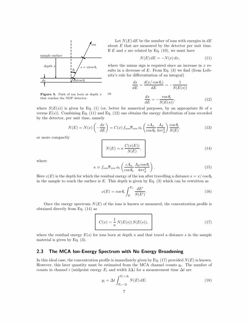
As seen from Fig. 5, the number of ions born in dx about x that reach the detector must travelthrough a distance s = x/ cos θs in the sample before reaching the surface and streaming to thedetector. The energy of these escaping ions born at depth x, E(x), is given by Eq. (1), i.e.,
s =x
cos θs=∫ Eo
E(s)
dE′
S(E′). (10)
6
sample surface
dx
depth x
dx/cos θs
s = x/cos θsθs
ion
Figure 5. Path of ion born at depth xthat reaches the NDP detector.
Let N(E) dE be the number of ions with energies in dEabout E that are measured by the detector per unit time.If E and x are related by Eq. (10), we must have
N(E) dE = −N(x) dx, (11)
where the minus sign is required since an increase in x re-sults in a decrease of E. From Eq. (3) we find (from Leib-nitz’s rule for differentiation of an integral)
ds
dE=
d(x/ cos θs)dE
= − 1S(E(s))
ordx
dE= − cos θs
S(E(s)), (12)
where S(E(s)) is given by Eq. (1) (or, better for numerical purposes, by an appropriate fit of sversus E(s)). Combining Eq. (11) and Eq. (12) one obtains the energy distribution of ions recordedby the detector, per unit time, namely
N(E) = N(x)(− dx
dE
)= C(x) fionσion φt
(εAn
cos θn
Ad
4πr2d
)cos θsS(E)
. (13)
or more compactly
N(E) = κC(x(E))
S(E), (14)
where
κ ≡ fionσion φt
(εAn
cos θn
Ad cos θs4πr2
d
). (15)
Here x(E) is the depth for which the residual energy of the ion after travelling a distance s = x/ cos θdin the sample to reach the surface is E. This depth is given by Eq. (3) which can be rewritten as
x(E) = cos θs
∫ Eo
E
dE′
S(E′). (16)
Once the energy spectrum N(E) of the ions is known or measured, the concentration profile isobtained directly from Eq. (14) as
C(x) =1κ
N(E(s))S(E(s)), (17)
where the residual energy E(s) for ions born at depth x and that travel a distance s in the samplematerial is given by Eq. (3).
2.3 The MCA Ion-Energy Spectrum with No Energy Broadening
In this ideal case, the concentration profile is immediately given by Eq. (17) provided N(E) is known.However, this later quantity must be estimated from the MCA channel counts yi. The number ofcounts in channel i (midpoint energy Ei and width 2∆) for a measurement time ∆t are
yi = ∆t
∫ Ei+∆
Ei−∆
N(E) dE. (18)
7

This result can also be written in terms of the concentration profile C(x) by substituting Eq. (13)into Eq. (18). The result
yi = ∆t
∫ Ei+∆
Ei−∆
N(E) dE = κ∆t
∫ Ei+∆
Ei−∆
C(x(E))S(E(s))
dE
= κ∆t
∫ x(Ei+∆)
x(Ei−∆)
C(x)S(E(s))
(dE
dx
)dx = κ∆t
∫ x(Ei+∆)
x(Ei−∆)
C(x)S(E(s))
(−S(E(s))
cos θd
)dx
=κ∆t
cos θd
∫ x(Ei−∆)
x(Ei+∆)
C(x) dx. (19)
This last result can readily be written in the following general convolution form, whose inversion isconsidered later in Section 4,
yi =∫ xmax
0
C(x)Ri(x) dx. (20)
where the channel response function is
Ri(x) =
⎧⎪⎨⎪⎩κ∆t
cos θd, x(Ei + ∆) < x < x(Ei − ∆),
0, otherwise.(21)
Here x(E) is the depth from which the residual ion energy at the sample surface is E after travelinga path length s = x/ cos θs. An empirical formula for this quantity is given by Eq. (5).
2.4 An Example Spectrum
The isotope 10B is readily detected by NDP because of its large thermal-neutron cross section (3840 bat 0.00253 eV) for the 10B(n,α)7Li reaction. Two distinct energies of α and 7Li ions are producedsince the 7Li nucleus is produced either in the ground state or in a 0.4776-MeV excited state asshown below.
10n + 10
5B −→⎧⎨⎩
73Li∗ + 4
2He (93.7%)
73Li + 4
2He (6.3%)
Alpha particles are produced with the two energies 1.7762 MeV (α1) and 1.4721 MeV (α2). Thecorresponding lithium ions have energies 1.0133 MeV (Li1) and 0.8398 MeV (Li2).
The National Institute of Standards and Technology (NIST) has prepared a reference NDPsample by implanting 10B ions into a silicon substrate. This sample, known as SRM-2137, has aaccurately measured 10B concentration profile, which is shown in Fig. 6.
NDP spectra calculated by Eq. (14) generally will exhibit peaks that are narrower than inspectra obtained experimentally. This is to be expected, since the result of Eq. (14) is based onthe assumption that all ions emitted at the same depth are recorded as having the same energy. Inreality, slightly different energies are recorded as a result of several non-idealizations. The treatmentof such energy broadening is the subject of the next section.
8

Figure 6. The 10B concentration profile for the NIST SRM-2137 referencesilicon waiver.
Figure 7. The ideal ion energy distribution as calculated by Eq. (14) without any energy broadeningfor the 10B distribution shown in Fig. 6.
9

2.5 Inversion of the MCA Spectrum
The inversion of Eq. (21) to obtain C(x) can be performed using the techniques discussed in Section 4.However, if the energy grid on the MCA spectrum is sufficiently fine such that N(E) varies onlyslightly over a channel width, a much simpler approach can be used. For this special case of a fineenergy mesh, Eq. (18) can be approximated as
yi = ∆t
∫ Ei+∆
Ei−∆
N(E) dE 2∆N(Ei)∆t, (22)
from which we have N(Ei) yi/(2∆ ∆t). Then from Eq. (17) we immediate obtain
C(xi) ≡ C(x(Ei)) =yi
∆t
S(Ei)2∆ κ
. (23)
An example of the estimated α2 ion peak in the MCA spectrum for the NIST SRM-2137 is shownin Fig. 8. This spectrum was obtained from numerical evaluation of Eq. (20) using the certified 10Bconcentration profile shown in Fig. 6. In inverted profile shown in Fig. 9 was obtained from Eq. (23).
3 NDP with Energy Broadening
In the ideal model of the previous section, the number of ions that escape the sample surface and aremeasured by the detector and that have a mean residual energy dE(s) about E(s) is from Eqs. (11)and (13)
N(E(s)) dE(s) = −[fionσion φt
(εAn
cos θn
Ad
4πr2d
)]C(x) dx ≡ −κC(x) dx, (24)
where κ ≡ κ/ cos θs, the constant in the square brackets.
The recorded energy of these ions will have a spread of energies about the mean residual energyas a result of (1) energy straggling as the ions travel through the sample material, (2) detector energybroadening caused by noise and the stochastic nature of ion reactions in the detector material, and(3) geometric broadening arising from the finite size of the detector and sample.
As ions travel through the sample material they undergo a myriad of stochastic interactionswith the ambient atoms losing slightly different amounts of energy even though they travel exactlythe same distance before reaching the surface. In addition, there are numerous small angle scattersthat cause ions to travel slightly different distances in the sample before reaching the surface and,thereby, having a spread of energies. These two effects on the energy spreading are collectivelyreferred to in this report as energy straggling.
The detector system itself broadens the measured ion energies as a result of its inherent resolu-tion. Three contributions can be identified: (1) electronic noise of the amplifier chain, (2) intrinsicnoise in the detector caused primarily by leakage currents, and (3) the stochastic variation in energydeposition by the ionizing interactions and stochastic competition with phonon production in thedetector material.
Although the detector and irradiated area of the sample are generally small, they, nevertheless,have finite sizes. Ions leaving the sample at slightly different angles and exit points can still reachthe detector. Thus, ions reaching the detector will have a distribution of path lengths in the sampleand, consequently, a distribution of energies when they leave the sample. This effect is referred toas geometric broadening.
10

Figure 8. The ideal spectrum N(E) and the predicted MCA spectrum forthe 1.4721-MeV α particle of the 10B(n,α)7Li reaction in the NIST SRM-2137silicon sample. The MCA spectrum was calculated from N(E) by numericallyevaluating Eq. (18).
Figure 9. The actual and unfolded concentration profile C(x) for the NISTSRM-2137 sample. The unfolded results were obtained using Eq. 23 and thepredicted MCA spectrum shown in Fig. 8.
11

3.1 Spectral Broadening from Energy Straggling
The broadening of ion energies caused by energy straggling was investigated using the Monte CarloTRIM code of the SRIM package [Ziegler and Biersack 2002]. For a specified thickness x of silicon,the exit energies of normally incident alpha and lithium ions were recorded (see Fig. 10. Based onN ≥ 10, 000 histories, the standard deviation of transmitted particle energies was computed as
σ2strag =
1N − 1
N∑i=1
(Ei − E)2, (25)
where Ei is the energy of the ith transmitted ion and the mean transmitted (residual) energy isE = (1/N)
∑Ni=1 Ei.
TRIM calculations of the energy straggling for the four ions produced in the 10B(n,α)7Li reactionwere made and the following empirical equation was fit to the calculated results.
σstrag
E= a + bEc. (26)
The empirical fit and the calculated energy straggling values are shown in Fig. 11. Values of thefitting parameters are given in Table 4.
Table 4. The initial energies, range in silicon, and the fit parameters forEq. (26) for the ions produced in the 10B(n,α)7Li reaction.
ionEo Range Parameters for Eq. (26)
(MeV) (µm) a b c
α1 1.7762 6.25 −.087053189 0.107157820 −0.37284172
α2 1.4721 5.11 −.084451428 0.098519784 −0.37706387
Li1 1.0133 2.81 −.035292668 0.043321774 −0.59331028
Li2 0.8398 2.49 −.049446492 0.048381691 −0.56563867
3.2 Detector Energy Broadening
The recorded energy by the MCA is directly proportional to the amplitude of the pulse receivedby the MCA. Thus, any phenomenon that stochastically (or deterministically) varies the pulseamplitude will cause an apparent broadening of the recorded energies. For the NDP detector systemthere are two energy-broadening effects (1) system noise (σnoise) and (2) stochastic variation of theamount of ionization produced by an ion in the detector crystal (σion). The overall variance of thedetector energy broadening is thus
σ2det = σ2
noise + σ2ion. (27)
The presence of noise in the detector and the amplifier chain perturbs the pulse amplitudesproduced by the detector crystal, thereby, leading to a broadening of the recorded energy spectrum.The amount of the energy broadening is usually the same for all ion energies, i.e., σnoise constant.
On the other hand, the stochastic competition between phonon production and ionization byions in the detector crystal produces different numbers of ionizing events for incident ions of thesame initial energy. Because the detector pulse amplitude is directly proportional to the number ofionization event cause by the incident ion, the detector produces different pulse amplitudes leading to
12

Figure 10. The distribution of energies of the α2 ion from the 10B(n,α)7Li reaction after travelingvarious distances in silicon. Each probability distribution was obtained using 10,000 histories fromthe TRIM simulation.
Figure 11. TRIM results for σstr/E (circles) and the empirical fit of Eq. (25)(lines). The vertical dashed lines indicate the range in a silicon of each ion.
13

an apparent spread of ion energies. The magnitude of the spread, or variance σ2ion, of this stochastic
ionization effect depends on the energy and charge of the ion as well as the detector material. Formost solid state detectors there is negligible phonon production produced by ions of the hydrogenisotopes, and hence σion constant [Maki et al. 1986]. For ions with a charge greater than one,σion generally cannot be neglected and is usually a function of the incident ion energy.
To determine the total detector system’s energy broadening, σ2det = σ2
noise + σ2ion, one gener-
ally must measure it by recording the MCA spectrum of monoenergetic ions of different energies(produced, say, by NDP measurements of a sample with a thin surface deposit of an ion producingisotope). In Fig. 12 we show a typical alpha peak produced by a sample with a surface coating ofboron. Also shown are various Gaussian distribution fits to the data.
Figure 12. The geometric energy broadening for the 1.47-MeV α2 ions pro-duced in the 10B(n,α)7Li reaction. The circles are measured data and the linesare Gaussian distribution fits to the data using different methods and numberof data.
3.2.1 Fitting a Gaussian Distribution to MCA Data
To determine the MCA system energy broadening variance σdet it is necessary to fit a Gaussiandistribution
y(E) = A exp[− (E − Ep)2
2σ2
](28)
to the MCA peak produced by an incident monoenergetic ion. Here the MCA data are the channelcounts yn ≡ y(En), n = 1, ..., N . Thus, we seek the Gaussian parameters A, Ep, and σ which givesthe “best” agreement between the Gaussian distribution. Two methods are proposed.
Linear Transformation. In this method, the first step is to estimate the peak amplitude A and itslocation Ep. A simple way is to fit a quadratic equation y(E) = a + bE + cE2 to the peak channelcount and the two bracketing channel counts ym−1, ym, ym+1. The location of the maximum of
14

y(E) is then Emax = −b/(2c) Ep and the peak value is y(Emax) = a + bEmax + cE2max A. Other
more sophisticated method for estimating Ep and A can be used, but seldom seem worth the effort.
With estimated values for Ep and A, the standard deviation can be found by taking the logarithmof Eq. (28) and manipulating the result to obtain
G(E) ≡ ±√
2 ln(
A
y(E)
)=
E
σ− Ep
σ. (29)
The +(−) sign in this result is used when E > Ep (E < Ep). Plotting G(E) versus E (or equivalently,plotting G(En) versus n) yields a straight line whose slope is 1/σ. The light lines in Fig. 12 wereobtained in this manner.
Nonlinear Least Squares Fit. The above technique is rather ad hoc. A more rigorous approachis to perform a nonlinear fit by finding the values of A, Ep and σ than minimize the chi-squaredstatistic
χ2 =N∑
n=1
[yn − y(En)
σn
]2, (30)
where y(E) is given by Eq. (28) and σn √yn is the standard deviation of the count in channel n.
This nonlinear minimization problem is readily perform numerically by using the mrqmin algorithmgiven by Press et al. [1992]. In Fig. 12 the heavy line shows the result of using a nonlinear leastsquares fit to the MCA data.
3.3 Spectral Broadening from Geometry Effects
Because of the finite sizes of the irradiated area of the sample and the detector, ions born at thesame depth in the sample can travel in different directions and still reach the detector (see Fig. 13).The detected ions will therefore have slightly different residual energies as a result of having traveleddifferent distances in the sample. This is the origin of geometric energy broadening.
We consider two cases. The first assumes the plane of the detector and the sample are parallel.Then a general formulation is presented in which the detector and sample planes can have arbitraryorientations.
3.3.1 Case of Parallel Sample and Detector Planes
To quantify the geometry effect for this particular geometry, consider a sample with an irradiatedsurface area As and a parallel detector plane of area Ad separated by a perpendicular distance h. Asshown in Fig. 14, ions born at depth t in a differential area dAs of the sample can reach a differentialarea dAd of the detector by traveling along a ray at angle θ to the surface normal. The probabilityan ion born isotropically at dAs will hit the detector element dAd is the fraction of 4π steradiansthat the solid angle dΩ subtended by dAd at dAs, namely dΩ/4π = (dAd cos θs)/4πr2). The numberof ions born at dAs and that reach dAd per unit time is thus
dN = ν dAs
(dAd cos θs
4πr2
), (31)
where ν is rate of ion emission per unit area at depth t. These ions reaching dAd all have a residualenergy E(s) where the sample path length is s = t/ cos θs. The energy spectrum (number per unitenergy) of these detected ions is then
dN(t, E) = ν
(cos θs4πr2
)dAs dAd δ(E − E(s)), (32)
15

detector
ions born at depth x
sample surface
s1s2 s3
Figure 13. Geometric energy broadening occurswhen ions born at the same depth can have differentpath lengths an still reach the detector.
sample surface
dAs (xs, ys, zs)
dAd
(xd, yd, zd)z
t
θs
r
Figure 14. Geometry for estimating the geometryenergy broadening effect. Ions born in dAs travel adistance s = t/ cos θs to reach a differential area dAd
of the detector.
where δ(E − E(s)) is the Kronecker delta function indicating that these ions are monoenergetic. Ifwe select the outward normal to the sample surface as the z-axis, and if (xs, ys, zs) and (xd, yd, zd)are the coordinates of dAs and dAd, respectively, then in Eq. (32) we have
r2 = (xd − xs)2 + (yd − ys)2 + (zs − zd)2
cos θs = (zd − zs)/r h/r
s = t/ cos θs t r/h.
Finally, the energy spectrum of all ions born at depth t across the irradiated area As and that reachthe detector of area Ad is obtained by integrating Eq. (32) over all dAs and dAd, namely
N(t, E) = ν
∫As
dAs
∫Ad
dAdcos θs4πr2
δ(E − E(s)). (33)
This equation can be evaluated numerically by subdividing As and Ad into a set of small ∆Asi
and ∆Adj and replacing the integrals by the appropriate finite summations. An example resultshowing the geometric energy broadening is shown in Fig. 15. Notice that the energy broadening is amonotonic increasing distribution from the smallest energy (produced by the longest ion path) to thehighest energy (produced by ions traveling the shortest perpendicular distance). For this example,it is seen that geometric energy broadening is relatively small compared to energy straggling anddetector resolution effects.
From Eq. (33) we can obtain the moments of the energy distribution as
En ≡ 〈En〉 ≡∫
EnN(t, E) dE
/∫N(t, E) dE. (34)
Substitution of Eq. (33) into this definition gives
En =∫
As
dAs
∫Ad
dAd En(s)cos θs
r2
/∫As
dAs
∫Ad
dAdcos θsr2
. (35)
16

Figure 15. The geometric energy broadening for α2
ions produced in the 10B(n,α)7Li reaction at a depthof 4 µm in silicon. Here the silicon sample and detectorare 1-cm squares separated by 10.8 cm.
Figure 16. The probability the α2 ions produced inthe 10B(n,α)7Li reaction reaches the detector in unitcosine about the direction ω = cos θ. Here the siliconsample and detector are 1-cm squares separated by10.8 cm.
The average energy of an ion reaching the detector from a depth t in the sample is then
Eav = 〈E〉 = E1, (36)
and the variance in the energies is
σ2geom = 〈(E − Eav)2〉 = E2 − E2
1 . (37)
3.3.2 Emission Distribution for Parallel Samples and Detectors
The energy broadening produced by the geometry effect (e.g., Fig. 15) is generally poorly describedby a Gaussian model and thus cannot be combined with other energy broadening effects into a singleGaussian distribution. Thus, geometric effects must be treated separately in describing the MCAion-energy spectrum. This would appear to be an exceedingly difficult task, since from Eq. (33),N(t, E) would have to be computed for an infinity of depths t at which ions are emitted in thesample.
However, an important observation can greatly simplify treating the geometry effect. The dis-tribution g(θ) of ion directions that reach the detector, as measured by θ or ω ≡ cos θ, is independentof t because t is negligible (micrometers) compared to the sample-detector separation (centimeters)[Cloakley et al. 1995]. The residual energy of an ion born at depth t and traveling to the detectorat an angle θs is readily computed as E(s) = E(t/ω).
With the same argument used to obtained Eq. (32), the number of ions born in dAs that reachdAd within unit cosine about ω ≡ cos θ is
dN(t, ω) dN(ω) = ν( ω
4πr2
)dAs dAd δ(ω − ωs(rs, rd)), (38)
where ω(rs, rd) is the cosine of the angle between the surface normals and the line joining dAs (atlocation rs) and dAd (at location rd). The number of ions reaching the detector from the sample in
17

unit cosine about the direction ω is then obtained by integrating the result over all dAs and dAd,namely
N(ω) = ν
∫As
dAs
∫Ad
dAdω
4πr2δ(ω − ωs(rs, rd)). (39)
This result can be readily evaluated numerically by subdividing As and Ad into sets of contiguouspixels of size ∆As and ∆Ad and replacing the integrals by appropriate summations.
Finally, the probability an ion born at any depth (with path length less than the ion’s range)reaches the detector within unit cosine about the direction ω is computed as
g(ω) =N(ω)νAs
(40)
where νAs is the total number of ions born at depth t. Usually, The detector and sample areasare small compared to the sample-detector distance, and, consequently, N(ω) and g(ω) are zeroexcept for a narrow range of ω. We denote by ωmin and ωmax the minimum and maximum cos θspermitted by the size and location of the detector and sample surfaces. The directional distributiong(ω) corresponding to the geometric energy broadening of Fig. 15 is shown in Fig. 16.
3.3.3 Case of Arbitrary Orientation of Detector and Sample Planes
rs
rd
rd−rs
x
z
y
dAs
θs
ns
sample
dAd
θdnd
detector
Figure 17. Two differential elements ofarea of the sample and detector surfaceswith arbitrary orientation to each other.
Consider a differential element of area dAs of the samplesurface which has a unit normal ns and is located at positionrs as shown in Fig. 17. A differential element of the detectorsurface dAd has a unit normal nd and is located at positionrd. The probability an ion emitted isotropically from dAs
heads in a direction that intersects dAd is
Pd =dΩd
4π=
dAd cos θd
4π|rd − rs|2 =nd•(rs − rd)4π|rd − rs|3 dAd. (41)
Here dΩd is the solid angle subtended by the detector sur-face element dAd at the sample element dAs. The cosine ofthe emission angle ωs ≡ cos θs is given by
ωs(rs, rd) =ns•(rd − rs)|rd − rs| . (42)
If ν denotes the number of ions emitted per unit sample surface area, the number of ions emittedfrom dAs in unit cosine about ω and that reach dAd is
dN(ω) = ν dAsnd•(rs − rd)4π|rd − rs|3 δ(ω − ωs(rs, rd))dAd. (43)
Integration of this result over the detector and sample surfaces then gives the number of ions emittedin unit cosine about ω from the sample that reach the detector as
N(ω) = ν
∫As
dAs
∫Ad
dAdnd•(rs − rd)4π|rd − rs|3 δ(ω − ωs(rs, rd)). (44)
Finally, division by the total number of ions born at depth t gives the probability distributionfunction g(ω) ≡ g(cos θ) that an ion reaching the detector leaves the sample in unit cosine aboutdirection ω, namely
g(ω) = N(ω)/νAs. (45)
If the detector and source planes are parallel, then θs = θd and Eq. (44) becomes the same asEq. (39). An example of a directional distribution function is shown in Fig. 18.
18

Figure 18. An example probability distribution for the emission directiong(ω). This result is for the example given by Croakley et al. [1995]. Thedetector is a 2.5-mm radius disk, the detector a 0.1-cm × 0.8-cm rectanglerotated by 70 degrees from the sample normal. The long edge of the detectoris perpendicular the rotation plane, and the detector plane is perpendicular tothe line between the sample and detector centers.
3.4 Importance of the Different Energy Broadening Effects
If we assume that all energy broadening effects can be adequately described by Gaussian-like be-haviors, then the probability an ion born at depths in dt about t = s cos θs is recorded by thespectrometer as having an energy in dE about E is
R(E(s), E) dE =1√
2πσ(s)exp[− (E(s) − E)2
2 σ2(s)
], (46)
where σ(s) is the standard deviation of all the energy broadening effects for an ion with path lengths in the sample. If σk(s) is the standard deviation of the kth broadening effect, then
σ(s) =√∑
k
σ2k(s). (47)
In practice, only energy straggling and the detector energy broadening effects are well describedby a Gaussian model. The energy broadening caused by the geometry effect is decidedly non-Gaussian and must be treated explicitly (see the next section). However, in many practical casesthe geometry effect can be ignored compared to the other two energy broadening effects. In thisexample we give a comparison of the importance of the three effects.
Estimates for KSU’s NDP facility have been made for σstrag as described in Section 3.1 and forσgeom as calculated from Eq. (37) for alpha particles born at different depths in silicon. However,only the a single experiment result for σdet has been made using a 1.47-MeV alpha particle. The fitsto the MCA data shown in Fig. 12 yield values for σdet 19.0 keV. How this values varies as theenergy of the alpha particle changes is presently unknown. Thus, for lack of other data, we assumeσdet = 19 keV for alpha particles emitted at all depths in the sample.
The variation of σdet with sample depth for α2 particles from the 10B(n,α)7Li reaction is shownin Fig. 19 along with the variation of its components.
19

Figure 19. The various contributions to the total standard deviation of theenergy broadening mechanisms for alpha particles in a typical NDP system.
3.5 NDP Spectra with Energy Broadening
The probability an ion born at depth x in the sample is emitted in dω about direction ω ≡ cos θwith respect the surface normal that intersects the detector surface is denoted by g(ω) (see Sections3.3.1 and 3.3.3). Because the depth x is almost always negligible compared to the sample-detectorseparation distance, this distribution is independent of x [Coakley et al. 1995].
Ions emitted at depth x in direction ω (see Fig. 5) travel a path length s = x/ω in the samplematerial and reach the detector with a mean residual energy E(s). If we assume a Gaussian modelfor energy broadening from both energy straggling and detector effects, the probability such an ionis recorded with energy in dE about E is
R(E, E(s), σ(s)) dE =1√
2πσ(s)exp[− (E − E(s))2
2 σ2(s)
]dE, (48)
where σ2(s) = σ2det +σ2
strag. With this energy broadening model, the probability p(x, E) dE that anion born at depth x in the sample is recorded with an energy in dE about E is
p(x, E) dE =[∫ ωmax
ωmin
g(ω)R(E, E(x/ω), σ(x/ω)) dω
]dE. (49)
If C(x) denotes the concentration at depth x of the trace isotope that produces the ion, thenfrom Eq. (7) the number of ions produced in dx about x is
Nion(x) dx = Fion(x)∆V = C(x) fionσion Φt
(An
cos θn
)dx = κ C(x) dx, (50)
where the thermal neutron fluence incident on the sample in measurement time ∆t is Φt = φt∆t,and κ ≡ fionσion ΦtAs since As = An/ cos θn.
20
With the results of Eqs. (49) and (50), the number of ions born at depths dx about x andsubsequently recorded by the MCA with energies in dE about E is
dy(E) dE = [Nion(x) dx] p(x, E) dE = κC(x) dx p(x, E) dE. (51)
The number born at all depths that are recorded with energies in dE about E is thus
y(E) = κ
∫ xmax
0
C(x)p(x, E) dx. (52)
Finally, the number of counts recorded in bin i of the MCA energy spectrum (bin width 2∆ andmidpoint energy Ei) is
yi =∫ Ei+∆
Ei−∆
y(E) dE = κ
∫ xmax
0
dxC(x)∫ Ei+∆
Ei−∆
dE p(x, E). (53)
This may be written as
yi =∫ xmax
0
C(x)Ri(x) dx i = 1, . . . , N, (54)
where the channel response function is defined as
Ri(x) = κ
∫ Ei+∆
Ei−∆
dE p(x, E)
= κ
∫ ωmax
ωmin
dω g(ω)∫ Ei+∆
Ei−∆
dE R(E, E(x/ω), σ(x/ω))
= κ
∫ ωmax
ωmin
dω g(ω)Wi(x/ω). (55)
Here the so-called spread function Wi(x/ω) is defined as
Wi(s) ≡∫ Ei+∆
Ei−∆
dE R(E, E(s), σ(s))
=12
[erf(
Ei + ∆ − E(s)√2 σ(s)
)− erf
(Ei − ∆ − E(s)√
2 σ(s)
)]. (56)
Special case of Good Geometry: In many NDP facilities, the geometry for obtaining the MCAion-energy spectrum is such that energy spreading from the geometry effect is very small compared toenergy straggling and detector resolution effects. See, for example, the KSU NDP results of Fig. 19.In such cases, the direction distribution function g(ω) can be approximated by a delta function, i.e.,g(ω) δ(ω −ωs) where ωs is the angle between the sample normal and the ray between the centersof the sample and detector (see Fig. 14). Under this approximation
Ri(x) κ
∫ ωmax
ωmin
δ(ω − ωs)Wi(x/ω) dω = κWi(x/ωs)
=κ
2
[erf(
Ei + ∆ − E(x/ωs)√2σ(x/ωs)
)− erf
(Ei − ∆ − E(x/ωs)√
2σ(x/ωs)
)]. (57)
Example response functions are shown in Figs. 20 and 21.
21

Figure 20. The MCA channel response function for the 1.4721-MeV α particleof the 10B(n,α)7Li reaction in a silicon sample. Only the energy stragglingcomponent of energy broadening is considered.
Figure 21. The MCA channel response function for the 0.8398-MeV lithiumion of the 10B(n,α)7Li reaction in a silicon sample. Only the energy stragglingcomponent of energy broadening is considered.
22

3.6 Numerical Evaluation of the MCA Ion Energy Spectrum
Both for comparison to experimental data with NDP standards samples and for testing deconvolutionor unfolding techniques to obtain the concentration profile C(x) from the MCA spectral data, it isimportant to be able to compute the expected MCA spectrum for a specified profile. In this sectionwe discuss several algorithms for this spectrum construction.
The expected number of counts in channel i of the MCA spectrum is given by Eq. (54). Thisintegral can be approximated by an appropriate weighted sum of concentrations at discrete depthsin the sample by using some quadrature approximation for the integral. Suppose we are given theconcentration at M equispaced depths xj such that x1 = 0 and xM = xmax, the depth beyond whichan ion cannot escape the sample. The concentration at depth xj is denoted by cj ≡ C(xj). Withthis discrete spatial grid, Eq. (54) is decomposed into a sum of integrals over the subintervals as
yi =∫ xmax
0
dxRi(x)C(x) =M−1∑j=1
∫ xj+1
xj
dxRi(x)C(x). (58)
Each integral in Eq. (58) is then evaluated by numerical quadrature to express the integrals in termof the cj. The resulting linear equations can be written as
yi =M∑
j=1
Rijcj , i = 1, ..., N (59)
or in matrix notationy = R•c. (60)
This result represents N equations in the M unknowns cj. Here the N × M matrix R dependson the numerical quadrature approximation selected to evaluate Eq. (58). Three possible schemesare presented below.
3.6.1 An Interval-Average Approximation
In this discretization, C(x) in each of the subintervals is approximated by the average of its endpointvalues. Thus Eq. (58) becomes
yi M−1∑j=1
cj+1 + cj
2
∫ xj+1
xj
Ri(x) dx
=M−1∑j=1
cj+1 + cj
2Qi,j
≡M∑
j=1
Rijcj (61)
where the elements of the R matrix are given by
Rij =12
⎧⎪⎪⎨⎪⎪⎩Qi,1, j = 1
Qi,j−1 + Qi,j , j = 2, . . . , M − 1
Qi,M−1, j = M
(62)
23

and
Qi,j ≡∫ xj+1
xj
Ri(x) dx.
The evaluation of Qi,j generally must be performed numerically.
3.6.2 A Piece-Wise Linear Approximation
In this approximation we assume C(z) varies linearly between its values at the endpoints of eachsubinterval, i.e.,
C(x) (xj+1 − x)cj/∆j + (x − xj)cj+1/∆j , xj ≤ x ≤ xj+1, (63)
where ∆j ≡ (xj+1−xj). Substitution of this linear approximation into Eq. (58) gives Eq. (59) wherethe Rij are given by
Rij =
⎧⎪⎪⎪⎪⎪⎪⎪⎪⎪⎨⎪⎪⎪⎪⎪⎪⎪⎪⎪⎩
∫ x2
x1
dz f1(x)Ri(x), j = 1
∫ xj+1
xj−1
dx fj(x)Ri(x), j = 2, . . . , M − 1
∫ xM
xM−1
dx fM (x)Ri(x), j = M
(64)
where the weighting functions fj(x) are defined as
fj(x) =
⎧⎪⎪⎨⎪⎪⎩(x − xj−1)/∆j−1, xj−1 ≤ x < xj
(xj+1 − x)/∆j , xj ≤ x < xj+1
0, otherwise.
(65)
The integrals in Eq. (64) generally must be evaluated using numerical integration.
3.6.3 A Piece-Wise Quadratic Approximation
Equation (54) can also be approximated by
yi =∫ xmax
0
dxRi(x)C(x) =M−2∑j=1
′∫ xj+2
xj
dxRi(x)C(x), (66)
where the prime on the summation indicates that the summation is over only odd values of j. For theapproximation developed here, M is assumed odd. Now approximate C(x) in each pair of adjacentsubintervals by a quadratic function. For equally spaced nodes with ∆ = xj+1 −xj , C(x) in interval(xj , xj+2) is approximated by
C(x) (x − xj+1)(x − xj+2)2∆2
cj − (x − xj)(x − xj+2)∆2
cj+1 +(x − xj)(x − xj+1)
2∆2cj+2. (67)
24

Substitution of this result into Eq. (66) gives Eqs. (59) where the Rij are now given by
Rij =1
2∆2
⎧⎪⎪⎪⎪⎪⎪⎪⎪⎪⎪⎪⎪⎪⎪⎪⎪⎪⎪⎪⎪⎪⎨⎪⎪⎪⎪⎪⎪⎪⎪⎪⎪⎪⎪⎪⎪⎪⎪⎪⎪⎪⎪⎪⎩
∫ x3
x1
dx (x − x2)(x − x3)Ri(x), j = 1
∫ xj
xj−2
dx (x − xj−2)(x − xj−1)Ri(x)
+∫ xj+2
xj
dx (x − xj+1)(x − xj+2)Ri(x), j odd, j = 1, M
−2∫ xj+1
xj−1
dx (x − xj−1)(x − xj+1)Ri(x), j even
∫ ZM
xM−2
dx (x − xM−2)(x − xM−1)Ri(x), j = M
(68)
3.7 Examples of Reconstructed MCA Spectra
In Fig. 22 two 256-channel MCA ion spectra are shown for NIST’s SRM-2137 10B implanted sample.The spectrum with energy straggling, but without any geometric energy broadening, was calculatedfrom Eq. (59) using the interval average approximation of Section 3.6.1 with M = 65 equispaced xj
between x = 0 and 0.320 µm (the values at which NIST tabulates the 10B concentration). Noticethat for this example, energy straggling is negligible since all the 10B is within 0.32 µm of thesample surface and, for such depths, energy straggling is negligible as can be seen from the extremenarrowness of the α2 response function in Fig. 20 for x < 0.3 µm.
Another possible NDP profile problem is to analyze a sample with a constant 10B concentrationthroughout the sample. Such, for example would be a sample of Pyrex (borosilicate) glass. InFig. 23 two predicted MCA ion-energy spectra are shown, one for a constant 10B concentration atall depths and a second for the case the 10B is constrained to a sublayer between 1 and 2.5 µm belowthe surface and zero otherwise. Energy straggling is apparent in this second spectrum as evidencedby a more gradual drop off of the α2 component around 0.9 MeV compared to its abrupt rise around1.4 MeV. Both spectra were also calculated from Eq. (59) using the interval average approximationof Section 3.6.1 with M = 400 equispaced xj between x = 0 and 6 µm.
4 The Unfolding Problem: Recovering the Concentration Profile
The observed counts in channel i of the ion energy spectrum is generally related to the concentrationprofile C(x) by Eq. (54), i.e.,
yi =∫ xmax
0
C(x)Ri(x) dx i = 1, . . . , N, (69)
where the channel response function Ri(x) depends on the model used to predict the energy distrib-ution of the ions reaching the detector. For the case of no energy broadening, this response functionif given by Eq. (21). For the case of energy broadening described by a Gaussian distribution aboutthe mean residual energy (see Section 3.5), the channel response function is given by Eq. (55) or byEq. (57) if geometric effects can be ignored.
25

Figure 22. The MCA ion energy spectrum for NIST’s SRM-2137 (see Fig. 6 for 10B concentrationprofile) The line is the spectrum without any energy broadening (the same as shown in Fig. 7), andthe circles show the spectrum with energy straggling included.
Figure 23. The predicted MCA ion spectrum for a sample with C(x) = Co
for all x (light line), and for C(x) = Co only for 1 < x < 2.3 µm.
26

The solution of Eq. (69) for the concentration profile is an inversion problem encountered inmany diverse fields. For example, this same inversion problem, but with different kernels, is en-countered in oil-well logging, neutron scattering, geophysical data analysis, atmospheric remotesensing, astrophysics, medical tomography, and many other data analysis applications. The solutionof Eq. (69) for C(x) given the N MCA channel counts yi, however, is a very ill-posed problem sincewe can have an infinite number of unknown values of C(x) between x = 0 and x = xmax and only afinite number of known yi.
In most inversion schemes, the Fredholm integral equation of Eq. (69) is approximated by a setof M algebraic equations for the concentration at M equispaced discrete depths in the sample (seeSection 3.6), namely
yi =M∑
j=1
Rijuj , i = 1, ..., N, (70)
where uj ≡ C(xj) and the Rij depend on the quadrature approximation used.2 In matrix notation,these equations may be written as
y = R•u. (71)
The inversion of Eqs. (70) generally has no unique solution since the number of unknowns M(the uj) is most likely different from the number N of measured data (the yi).
If M < N (more equations than unknowns) the problem is over-determined and generally nosolution exists. By contrast, if M > N (more unknowns than equations) there is an infinity ofsolutions because the solution space (of dimension M) has an (M − N) dimensional degeneracy,i.e., any (M − N) components of u can be specified arbitrarily and still have Eq. (70) satisfied.This under-determined case is typical of an NDP spectrum that is concentrated in only a few MCAchannels. The case with M = N , which has a unique solution, is very unlikely since selection ofthe MCA spectrum scale and the discretization of the concentration profile C(x) are usually doneindependently.
The question on how to extract a meaningful estimate of the concentration profile from Eqs. (70)is the subject of this section. Two approaches are presented: (a) a least-squares fitting technique,and (b) a linear regularization technique. However, before we consider these approaches, we firstconsider the ideal case of Section 2.2 in which there is no energy broadening of the NDP spectrum.
4.1 Unfolding Techniques for the NDP Problem
Several different approaches have been applied to estimate the concentration profile C(x) (or theuj ≡ C(xj) from the measured MCA channel counts yi.
4.1.1 Direct methods:
In this approach one attempts to describe the concentration profile by some known function G(x; ξ)with M parameters ξi. For example, one might think that the concentration profile could be wellapproximated by a four-parameter beta function
G(x; A, τ, α, β) = CoΓ(α + β)Γ(α)Γ(β)
τ1−α−βxα−1(τ − x)β−1, 0 ≤ 0 ≤ τ.
2In this section we use uj instead of cj to emphasize that the uj are the unknown quantities we are seeking. Similarlywe will use u(x) ≡ C(x) to denote the continuous concentration profile in the sample.
27

The amplitude parameter Co adjusts the magnitude of the profile and the positive shape parametersα and β allow this function to assume a wide variety of shapes over the interval (0,τ). Alternatively,one might assume the concentration profile is a piece-wise linear functions between M equidistancedepths in the sample, as was done in Section 3.6.2. In this case, the unknown parameters are theconcentrations ui at each depth – the very quantities that we are seeking!
Once a concentration model has been selected, a predicted MCA spectrum yi, i = 1, ...N canbe computed from Eq. (69) with C(x) replaced by the model G(x; ξ. One then selects the “best”values for the model parameters ξ by minimizing the disagreement between the measured data andthe predicted data. This is usually done by minimizing the statistic [Hoffman 1983]
χ2 =N∑
i=1
(yi − gi)2.
The direct approach often produces erratic results when there is significant noise in the data orif there is a large number of parameters to be estimated. However, it is this approach we shall studyin the following sections.
4.1.2 Iterative Methods:
Several iterative techniques have been used for unfolding MCA energy spectral data. Many are ad hocschemes whose mathematical properties, such as convergence, are not well established. Nevertheless,they often produce useful results, especially if the concentration profile is a slowly varying functionof x. We illustrate this approach with a simple iterative scheme proposed long ago by Cittert [1931]and used for NDP analysis by Maki et al. [1986].
This scheme is based on the formulation of Eq. (70), and with it a successive series of estimatesu
(n)i , n = 1, ... is obtained for the concentration ui. From Eq. (70), the error between the true value
and the nth estimate is
e(n)i ≡ yi −
M∑j=1
Riju(n)j (72)
A revised estimate of ui is obtained by adding this error term to the previous estimate, i.e.,
u(n+1)i = u
(n)i +
⎡⎣yi −M∑
j=1
Riju(n)j
⎤⎦ , n = 0, 1, ... (73)
In this scheme we see that if u(n)j is too large (or small) the error is negative (or positive) and a
corrector is thus subtracted (or added) to obtain the next estimate. The iteration is begun withu
(0)i = yi. After several iterations the error term consists mostly of noise, indicated by random sign
changes in e(n)i as i varies. The final estimate, after k iterations, is then obtained by “smoothing”
out the noise as [Wertheim 1975]
uestj = u
(k)j − k
⎡⎣yi −M∑
j=1
Riju(k)j
⎤⎦ . (74)
Critical to the success of this procedure is that both the data yi and the concentration profile besmooth and slowly varying.
28

4.1.3 Fourier Transform Methods
In Eq. (70) the response matrix elements Rij are narrowly peaked around i j, i.e., Rij is largewhen the residual energy from depth j is near the MCA channel energy Ei. Thus Eq. (70) can beviewed as a discrete convolution of a signal u(x) with a narrowly peaked response function. Usingthe convolution theorem for Fourier transforms [Press et al. 1992], the discrete Fourier transformof the uj can be obtained in terms of the discrete Fourier transforms of yi and Rij . Inversion thengives an estimate of uj.
The difficulty with Fourier transform techniques is that spurious features are often added to theunfolded profile as a result of aliasing errors produced by the relatively small amount of discretedata in the MCA spectrum.
4.2 Least-Squares: Over-Determined Set of Equations
For the case in which we have more data than unknowns, the usual procedure is to seek a solutionvector u that minimizes the difference between the data y and the MCA spectrum predicted bythe NDP model. This difference between a model and measured data is often quantified by the χ2
statistic, namely,
χ2 =N∑
i=1
M∑j=1
[yi −
M∑k=1
Rikuk
]S−1
ij
[yj −
M∑k=1
Rjkuk
](75)
N∑
i=1
1σ2
i
[yi −
M∑k=1
Rikuk
]2
= |A•u− b|2. (76)
Here Sij = Covar[ni, nj ] are the elements of the covariance matrix. The approximate equality in theabove result holds if we can neglect the off-diagonal covariance terms, with σ2
i = Covar[ni, ni]. Thematrix A has elements Aij = Rij/σi and the vector b has elements bi = yi/σi. For the countingdata of a MCA spectrum, the estimate of σi is
√yi provided yi is sufficiently large (namely, yi
>∼ 20).
The problem of finding the best agreement between the data and model is to find the vector uthat minimizes this χ2(y) statistic. Should we find a u such that χ2 = 0, then this is a “perfect”solution giving exact agreement between experiment and the model. However, such a solution seldomexists, particularly when the yi usually contain some random noise. The best we can do is to find au that minimizes χ2(y). Such a solution is often called the least-squares solution since it minimizesthe (weighted) sum of the squares of the differences between the data and model.
4.2.1 Least-Squares Solution
To obtain the least-squares solution, we seek the vector u that minimizes the χ2 of Eq. (76) whichcan be written as
χ2 =N∑
i=1
1σ2
i
⎡⎣yi −M∑
j=1
Rijuj
⎤⎦2
. (77)
At the minimum, ∂χ2/∂uk = 0. Differentiating the above equation gives
∂χ2
∂uk= 0 =
N∑i=1
2σ2
i
⎡⎣yi −M∑
j=1
Rijuj
⎤⎦Rik, k = 1, . . . , M, (78)
29

which givesM∑
j=1
N∑i=1
RijRik
σ2i
uj =N∑
i=1
yiRik
σ2i
, k = 1, . . . , M. (79)
These so-called normal equations can be written more compactly as
M∑j=1
αkjuj = βk, k = 1, . . . , M, (80)
where
αkj ≡N∑
i=1
RijRik
σ2i
and βk ≡N∑
i=1
yiRik
σ2i
. (81)
The normal equations, in matrix form, are thus
α•u = β, (82)
where the M × M matrix α = AT•A and the M -component vector β = AT•b.
Formally, the solution of Eqs. (82) can be written as
uk =M∑
k=1
α−1jk βk =
M∑k=1
α−1jk
[yiRik
σ2i
]. (83)
In practice, rather than generate the inverse matrix α−1, one solves the normal equations (Eqs. (82))directly. However, as Price et al. [1992] points out, the solution of these linear equations is very sus-ceptible to numerical roundoff errors and often the solution u obtained with, say, Gauss eliminationis often meaningless with adjacent components oscillating between enormous positive and negativevalues. The reason for this is that the normal equations are often nearly singular because differentcombinations of the Rij response matrix elements often fit the data equally well (or equally poorly).Consequently, the α matrix, unable to distinguish between nearly equal combinations, becomes closeto singular.
To avoid such spurious solutions of the normal equations, a different approach to finding theminimum of χ2 should be used. This approach is to perform the minimization using the singularvalue decomposition (SVD) technique. The algorithms and theory for this method are presentedby Price et al. [1992] and will not be repeated here. The solution that minimizes χ2 of Eq. (77) isreadily obtained with the subroutine svdfit presented by Price et al. [1992]. As an added bonus,this SVD method for minimizing χ2 can also be used for under-determined sets of equations!
4.3 Linear Regularization: Under-Determined Set of Equations
Minimization of the positive functional A[u] ≡ χ2 = |A•u − b|2 for a matrix A that is degenerate,i.e., has fewer rows than columns, will not give a unique solution for u. To obtain a unique solution,additional constraints must be imposed on the minimization problem. For example, if any non-degenerate strictly convex functional B[u], for example uT •H•u, is added, then the minimization ofA[u] + λB[u] will produce a unique solution u [Press et al. 1992]. The addition of the term λB[u] issaid to “regularize” the minimization problem, i.e., to produce a unique solution.
Thus in the inverse problem, to obtain a unique solution for u, one solves the following mini-mization problem
minimize: A[u] + λB[u]. (84)
30

This is the central principle of inversion theory. As the Lagrange multiplier λ varies from 0 to∞, the unique solution u varies from one minimizing A[u] to one minimizing B[u]. To obtain the“best” solution (corresponding to a particular value of λ) one must choose a particular criterion. Forexample, one might pick λ so that χ2 = N to agree with the expected value of χ2. Alternatively, onemight pick λ purely subjectively so as to produce, for example, a “smooth” solution or a solutionsensitive to abrupt changes in the profile u(x). Finally, for simulated NDP data obtained by accuratenumerical integration of Eq. (58), the most accurate inversion will be obtained with λ made as smallas possible, but still large enough to avoid numerical instabilities in the minimization algorithm.
The many apparently different approaches used for inversion problems by the regularizationtechnique all involve minimizing the functional of Eq. (84) with the choice for A[u] and B[u] de-pendent on the problem and the inversion philosophy. Such methods include the Backus-Gilbertand Maximum Entropy methods. These are not reviewed here; the interested reader is referred toPrice et al. [1992]. Rather I have found the linear regularization, the simplest of these regulariza-tion techniques, to be effective for the NDP unfolding problem. In essence this approach imposes asmoothness constraint on the solution. The linear regularization method and a constrained linearregularization approach are discussed in the following subsections.
4.3.1 The Linear Regularization (LR) Method
The linear regularization method goes by many names, for example, Tikhonov-Miller regularization[Tikhonov 1964; Tikhonov and Arsenin 1977; Miller 1970; Biemond et al. 1990], the Phillips-Twomeymethod [Phillips 1962; Twomey 1963], the constrained linear inversion method [Twomey 1977], andthe method of regularization [Craig and Brown 1986].). As with any method that has evolved frommany different disciplines, the notation and ideas in the many seminal works are often quite different.In the summary of this and the other inversion methods discussed in this paper, we adhere closelyto the notation of Press et al. [1992].
In the linear regularization approach, the functional A[u] of Eq. (84) is taken as the χ2 ofEq. (76), i.e., A[u] = |A•u− b|2, and the functional B[u] is chosen as some measure of the smooth-ness of u(x), which is derived from first or higher derivatives of u(x). In particular, the linear regu-larization method requires that B[u] = uT •H•u where H is some appropriate symmetric smoothingmatrix. The inversion solution is thus determined by the following minimization problem:
minimize: A[u] + λB[u] = |A•u − b|2 + λuT •H•u. (85)
The matrix H is obtained by making some a priori assumption about the nature of the concentrationprofile C(x) ≡ u(x). Several example smoothing matrices are presented in Section 4.3.2 below.
To obtain the minimum of the functional of Eq. (85) and find u, we write Eq. (85) in itscomponent form as
F [u] ≡ A[u] + λB[u] =N∑
i=1
⎡⎣ M∑j=1
Aijuj − bi
⎤⎦2
+ λ
M∑i=1
ui
M∑j=1
Hijuj. (86)
The values of uj that minimize this functional are the solutions of the M normal equations obtainby setting the derivative of F [u] with respect to uj to zero. Differentiation of Eq. (86) with respectto uj , setting the result to zero, and use of the symmetry property of H gives
M∑j=1
(N∑
i=1
AikAij
)+ λHkj
uj =
M∑i=1
Aikbi, k = 1, ..., M, (87)
31

or, in matrix form,
(AT •A + λH)•u = AT •b. (88)
This set of M linear algebraic equations is readily solved for u using standard techniques such asthe Lower-Upper (LU) decomposition method or the Singular Value Decomposition (SVD) method[Press et al. 1992].
Notice that before solving Eq. (88), one must first pick a value of λ. What value to pick? If theerrors σi are known reasonably well, one might pick λ so that the χ2 equals N . To obtain confidencebounds on u, λ could be chosen so that χ2 equals N±(2N)1/2. Thus the solution of Eq. (88) involvesa root finding process whereby λ is adjusted until χ2 attains some prescribed value. As a startingpoint for the λ search, Press et al. [1922] suggests
λ = Tr(AT •A)/Tr(H) (89)
where Tr is the matrix trace (sum of diagonal elements).
4.3.2 Smoothing Matrices
The construction of the M × M matrix H depends on the a priori smoothness criterion chosen.For example, if we believe that the concentration profile u(x) is approximately constant, then areasonable functional to minimize so as to enforce this belief is (assuming equispaced values of xj)
B[u] ∝∫ ∞
0
[u′(x)]2 dx ∝M−1∑j=1
[uj − uj+1]2 (90)
since this functional is nonnegative and vanishes only when u(x) equals a constant. The constantof proportionality can be absorbed into the parameter λ so that the discretized form of B[u] can bewritten as
B[u] = |B•u|2 = uT•(BT
•B)•u = uT•H•u, (91)
where B is the (M − 1) × M first-order, forward finite-difference matrix
B =
⎛⎜⎜⎜⎜⎜⎝−1 1 0 0 0 0 0 . . . 0
0 −1 1 0 0 0 0 . . . 0...
. . ....
0 . . . 0 0 0 0 −1 1 00 . . . 0 0 0 0 0 −1 1
⎞⎟⎟⎟⎟⎟⎠ , (92)
and H = BT •B is the M × M symmetric matrix
H =
⎛⎜⎜⎜⎜⎜⎜⎜⎜⎜⎝
1 −1 0 0 0 0 0 . . . 0−1 2 −1 0 0 0 0 . . . 0
0 −1 2 −1 0 0 0 . . . 0...
. . ....
0 . . . 0 0 0 −1 2 −1 00 . . . 0 0 0 0 −1 2 −10 . . . 0 0 0 0 0 −1 1
⎞⎟⎟⎟⎟⎟⎟⎟⎟⎟⎠. (93)
Although this choice of constant smoothing leads to a particularly simple form for the matrixH, it is unrealistic to suppose the contaminant concentration profile is almost a constant. Rather, it
32

would be better to assume that u(x) varies linearly, quadratically or as any some higher polynomialin x. Such different a priori assumptions leads to different B and H matrices. Below some morerealistic smoothing schemes are proposed.
Linear Smoothing If we believe a linear function is a good approximation for C(x) ≡ u(x) thenwith forward finite differences we should minimize
B[u] ∝∫ ∞
0
[u′′(x)]2 dx ∝M−2∑j=1
[−uj + 2uj+1 − uj+2]2 (94)
so that
B =
⎛⎜⎜⎜⎜⎜⎝−1 2 −1 0 0 0 0 . . . 0
0 −1 2 −1 0 0 0 . . . 0...
. . ....
0 . . . 0 0 0 −1 2 −1 00 . . . 0 0 0 0 −1 2 −1
⎞⎟⎟⎟⎟⎟⎠ , (95)
which yields for H = BT •B the M × M symmetric matrix
H = BT •B =
⎛⎜⎜⎜⎜⎜⎜⎜⎜⎜⎜⎜⎜⎜⎝
1 −2 −1 0 0 0 0 . . . 0−2 5 −4 1 0 0 0 . . . 0
1 −4 6 −4 1 0 0 . . . 00 1 −4 6 −4 1 0 . . . 0...
. . ....
0 . . . 0 1 −4 6 −4 1 00 . . . 0 0 1 −4 6 −4 10 . . . 0 0 0 1 −4 5 −20 . . . 0 0 0 0 1 −2 1
⎞⎟⎟⎟⎟⎟⎟⎟⎟⎟⎟⎟⎟⎟⎠. (96)
Quadratic Smoothing If we believe a quadratic function is a good approximation for u(x) then weshould minimize (again use forward finite differences)
B[u] ∝∫ ∞
0
[u′′′(x)]2 dx ∝M−3∑j=1
[−uj + 3uj+1 − 3uj+2 + uj+3]2 (97)
so that
B =
⎛⎜⎜⎜⎜⎜⎝−1 3 −3 1 0 0 0 . . . 0
0 −1 3 −3 1 0 0 . . . 0...
. . ....
0 . . . 0 0 −1 3 −3 1 00 . . . 0 0 0 −1 3 −3 1
⎞⎟⎟⎟⎟⎟⎠ , (98)
33

which yields for H = BT •B the M × M symmetric matrix
H = BT •B =
⎛⎜⎜⎜⎜⎜⎜⎜⎜⎜⎜⎜⎜⎜⎜⎜⎜⎜⎝
1 −2 −1 0 0 0 0 0 0 . . . 0−2 5 −4 1 0 0 0 0 0 . . . 0
1 −4 6 −4 1 0 0 0 0 . . . 00 1 −4 6 −4 1 0 0 0 . . . 00 1 −4 6 −4 1 0 0 0 . . . 0...
. . ....
0 . . . 0 −1 6 −15 20 −15 6 −1 00 . . . 0 0 −1 6 −15 20 −15 6 −10 . . . 0 0 0 −1 6 −15 19 −12 30 . . . 0 0 0 0 −1 6 −12 10 −30 . . . 0 0 0 0 0 −1 3 −3 1
⎞⎟⎟⎟⎟⎟⎟⎟⎟⎟⎟⎟⎟⎟⎟⎟⎟⎟⎠
. (99)
Second-Order Quadratic Smoothing The use of the first-order forward finite difference approxi-mation for u′′′(x) in Eq. (97) can be made more accurate for the nodes interior to the boundariesby using a second-order central difference approximation, i.e.,
u′′′i ∝ [−ui−2 + 2ui−1 − 2ui+1 + ui+2]/2, 2 < i < M − 1. (100)
With this approximation, and the first-order forward and backward finite difference approximationfor i = 1, 2, M − 1, M , the (M × M) B matrix becomes
B =
⎛⎜⎜⎜⎜⎜⎜⎜⎜⎜⎜⎜⎜⎜⎝
−2 6 −6 2 0 0 0 . . . 00 −2 6 −6 2 0 0 . . . 0
−1 2 0 −2 1 0 0 . . . 00 −1 2 0 −2 1 0 . . . 0...
. . ....
0 . . . 0 −1 2 0 −2 1 00 . . . 0 0 −1 2 0 −2 10 . . . 0 0 −2 6 −6 2 00 . . . 0 0 0 −2 6 −6 2
⎞⎟⎟⎟⎟⎟⎟⎟⎟⎟⎟⎟⎟⎟⎠. (101)
The resulting H = BT •B is the M × M symmetric matrix
H =
⎛⎜⎜⎜⎜⎜⎜⎜⎜⎜⎜⎜⎜⎜⎜⎜⎜⎜⎜⎜⎜⎜⎜⎜⎜⎜⎜⎝
5 −14 12 −2 −1 0 0 0 0 0 0 . . . 0−14 45 −50 20 0 −1 0 0 0 0 0 . . . 0
12 −50 77 −50 8 4 −1 0 0 0 0 . . . 0−2 20 −50 49 −16 −4 4 −1 0 0 0 . . . 0−1 0 8 −16 14 −4 −4 4 −1 0 0 . . . 0
0 −1 4 −4 −4 10 −4 −4 4 −1 0 . . . 00 0 −1 4 −4 −4 10 −4 −4 4 −1 . . . 0...
. . ....
0 . . . −1 4 −4 −4 10 −4 −4 4 −1 0 00 . . . 0 −1 4 −4 −4 10 −4 −4 4 −1 00 . . . 0 0 −1 4 −4 −4 14 −16 8 0 −10 . . . 0 0 0 −1 4 −4 −16 49 −50 20 −20 . . . 0 0 0 0 −1 4 8 −50 77 −50 120 . . . 0 0 0 0 0 −1 0 20 −50 45 −140 . . . 0 0 0 0 0 0 −1 −2 12 −14 5
⎞⎟⎟⎟⎟⎟⎟⎟⎟⎟⎟⎟⎟⎟⎟⎟⎟⎟⎟⎟⎟⎟⎟⎟⎟⎟⎟⎠
. (102)
34

Cubic Smoothing Finally, we present the smoothing matrix for cubic smoothing. If one uses first-order forward finite differences for the fourth derivative, with cubic smoothing one tries to minimize
B[u] ∝∫ ∞
0
[u′′′′(x)]2 dx ∝M−4∑j=1
[−uj + 4uj+1 − 6uj+2 + 4uj+3 − uj+4]2 (103)
so that
B =
⎛⎜⎜⎜⎜⎜⎝−1 4 −6 4 −1 0 0 . . . 0
0 −1 4 −6 4 −1 0 . . . 0...
. . ....
0 . . . 0 −1 4 −6 4 −1 00 . . . 0 0 −1 4 −6 4 −1
⎞⎟⎟⎟⎟⎟⎠ , (104)
which yields for H = BT •B the M × M symmetric matrix
H =
⎛⎜⎜⎜⎜⎜⎜⎜⎜⎜⎜⎜⎜⎜⎜⎜⎜⎜⎜⎜⎜⎜⎜⎜⎜⎜⎜⎝
1 −4 6 −4 1 0 0 0 0 0 0 . . . 0−4 17 −28 22 −8 1 0 0 0 0 0 . . . 0
6 −28 53 −52 28 −8 1 0 0 0 0 . . . 0−4 22 −52 69 −56 28 −8 1 0 0 0 . . . 0
1 −8 28 −56 70 −56 28 −8 1 0 0 . . . 00 1 −8 28 −56 70 −56 28 −8 1 0 . . . 00 0 1 −8 28 −56 70 −56 28 −8 1 . . . 0...
. . ....
0 . . . 1 −8 28 −56 70 −56 28 −8 1 0 00 . . . 0 1 −8 28 −56 70 −56 28 −8 1 00 . . . 0 0 1 −8 28 −56 70 −56 28 −8 10 . . . 0 0 0 1 −8 28 −56 69 −52 22 −40 . . . 0 0 0 0 1 −8 28 −52 53 −28 60 . . . 0 0 0 0 0 1 −8 22 −28 17 −40 . . . 0 0 0 0 0 0 1 −4 6 −4 1
⎞⎟⎟⎟⎟⎟⎟⎟⎟⎟⎟⎟⎟⎟⎟⎟⎟⎟⎟⎟⎟⎟⎟⎟⎟⎟⎟⎠
. (105)
4.3.3 Constrained Linear Regularization (CLR) Method
Often there are physical constraints on the unknown concentration profile u(x) ≡ C(x) which shouldalso be incorporated into the inversion process. For example, one may want u(x) ≥ 0 or uL(x) ≤u(x) ≤ uU(x) for specified bounding functions uL and uU . In the NDP problem, the concentrationprofile u(x) clearly must be non-negative. The method of projections onto convex sets [Biemond etal. 1990; Press et al. 1992] easily imposes such deterministic constraints if an iterative solution ofthe functional minimization problem is used.
Many iterative schemes can be used to find the u(x) that minimizes the functional A[u] +λB[u]. An unsophisticated approach is to use the method of steepest descent, whereby the minimumof A[u] + λB[u] is approached by proceeding from some arbitrary starting point in u space bytaking small steps always in the direction opposite the gradient of A[u] + λB[u], i.e., downhill.Mathematically, the iteration search is
u(k+1) = u(k) − ε∇(A[u] + λB[u]), (106)
where ε is a parameter that determines how far to move downhill in each step. For the linearregularization method, based on minimizing the functional A[u] + λB[u] = |A•u− b|2 + λuT •H•u
35

(see Eq. (85)), the minimization iteration scheme becomes
u(k+1) = u(k) − ε∇(|A•u − b|2 + λuT •H•u)
= u(k) − 2ε[(AT •A + λH)•u− AT •b]
= [1− ε(AT •A + λH)]•u(k) + εAT •b, (107)
where, to guarantee convergence [Press et al. 1992],
0 < ε <1
max eigenvalue (AT •A + λH). (108)
The converged solution limk→∞ u(k) will be the same as the LR solution obtained from Eq. (88).
To impose a non-negativity constraint on this iterative solution, define P as the projectionoperator that sets to zero all negative components of u. Then modify Eq. (107) to
u(k+1) = P[1− ε(AT •A + λH)]•u(k) + εAT •b, (109)
ensuring that, after each iteration, any negative components of u are set to zero. The convergedsolution of this equation is the vector with nonnegative components that minimizes A[u] + λB[u]using the linear regularization method.
4.3.4 Examples of Unfolded Concentration Profiles
Step-Discontinuous Profile
In Fig. 24 the α2 component of the MCA ion spectrum is shown for a sample with C(x) = 1019
atom/cm3 for 0 ≤ x ≤ 2 µm and zero below 2 µm. This spectrum was calculated using Eq. (70)and the interval average technique of Section 3.6.1. A 256 channel spectrum covering the ion energyrange of 0 to 2 MeV was used, and the simulated counts in at least N = 100 channels containingthe α2 component were used to unfold the concentration profile at M = 30 depths between 0 and 5µm. This is an example of an over-determined unfolding problem. Further a concentration profilewith a step discontinuity is a severe test of any inversion method.
The unfolded profile obtained with the SVD least squares method of Section 4.2.1 is shown inFig. 25. In this example the simulated counts in channels 90 to 190 (N = 101) were used. Forthis and other NDP unfolding problems, the normal equations for the least squares method are verynearly singular, and the SVD solutions of the normal equations overcomes this near degeneracynicely (compared to a Gauss elimination solution which gives meaningless results). However, eventhe SVD least squares profile, while finding the sharp cutoff at x = 2 µm, is seen to exhibit smallspurious oscillations about the exact profile.
The linear regularization (LR) method is designed for under-determined systems; however, it canalso be applied to this over-determined problem. In the LR results shown in Fig. 25, the simulatedcounts in channels 50–190 (N = 141) were used. From these results, the LR estimated profile has nospurious oscillations unlike the SVD-least-squares profile. However, at the dropoff at x = 2 µm theLR profile exhibits spurious over and under shoots near the discontinuity. This is largely due to thelinear smoothing with the H-matrix of Eq. (96) that was used in the calculations. When constantsmoothing is assumed these over and under shoots disappear.
The NIST SRM-2137 Sample
Based on the certified and tabulated 10B concentration in the NIST SRM-2137 sample, the expected256-channel MCA spectrum for the α2 ion was estimated over an energy range of 0 to 2 MeV. This
36

Figure 24. The simulated MCA spectrum for the α2 ion generated in a samplecontaining C(x) = 1019 10B atoms/cm3 for the first two micrometers and no10B for deeper depths.
Figure 25. The unfolded sample concentration for the simulated spectrumdata of Fig. 24. Results are shown for the SVD least squares method (circles)and for the linear regularization method (squares).
37

MCA spectrum was calculated using Eq. (70) and the interval average technique of Section 3.6.1.Because the 10B in SRM-2137 is distributed only within the first few tenths of µm, most MCAchannels had zero counts. Only channels 175–190 (corresponding to midpoint energies of 1.363–1.480 MeV) had non-zero counts. The estimated MCA spectrum is shown in the insert of Fig. 26.
The simulated data in channels 170–190 (N = 21) were then analyzed by the LR method toestimate the concentration profile at M = 30 sample depths between 0 and 0.5 µm. The solutionto this under-determined inverse problem is shown in Fig. 26 along with the certified profile. Theinclusion of the simulated data in channels 50–169 (all with zero counts) in addition to that in chan-nels 170–190 produced a highly over-determined problem (M = 141) but the LR method producedvirtually the same results.
In using the LR inversion technique, a value must be chosen for the parameter λ, which balancesthe trade off between agreement with the data (the χ2 term) and the smoothness constraint (theH-term) that regularizes the problem. In the results shown in Fig. 26, the value of λ given byEq. (89), namely λ = 0.020 was used. In these results, linear smoothing was used with the H-matrixgiven by Eq. (96). However, for 10−16 <∼ λ <∼ 10−3 almost the same results were obtained.
In Fig. 27 the variation of the χ2 and H terms at the minimum of Eq. (85) is shown as λ varies.The smaller χ2 the better is the agreement with the data while the smaller H the smoother isthe solution. For very large values of λ very smooth profiles are obtained at the expense of pooragreement with the data. By contrast, for very small values of λ, the profile agrees well with the datawhile the linear smoothness of the profile is compromised. However, if λ becomes too small (hereλ <∼ 10−16), The H-term contribution in Eq. (85) is lost in the round off of the computer calculationsand it ceases to regularize the under-determined set of equations and produces numerically unstablesolutions. These effects of extreme values of λ are shown in Figs. 28 and 29.
The large range of values that λ can assume and still give accurate estimates of the concentrationprofile is deceptive. These examples are for “perfect” data, i.e., data without any stochastic noise.The presence of noise in the data can generally be expected to reduce severely the λ range overwhich accurate results are produced. However, quantification of this effect is left for future work.Suffice it to say, that the LR method for inverting MCA NDP data to estimate the profile appearsto be robust both for the under determined problem (few MCA channels used) as well as for theover determined problem (many MCA channels used).
5 Conclusions
Methods for simulating NDP ion-energy spectra for the case of plane samples and detectors, witharbitrary orientation, have been presented. In particular, several phenomena which broaden or smearthe NDP spectra have been modeled, namely (1) energy straggling, (2) detector noise and stochasticenergy deposition, and (3) geometric energy broadening. Empirical methods for simulating the firsttwo of these effects have been presented, and a method, based on the emission-angle distributionhas been shown to be an efficient method for simulating the latter effect.
With these simulation techniques for estimating NDP spectra, several test spectra have beencalculated and used as a basis for testing the robustness of spectral unfolding or inversion techniques.Typically, NDP spectral inversions are over-determined problems if many MCA channels are used.For concentration profiles that are smoothly varying functions of depth, the linear regularization(LR) method is shown to work well for both over-determined and under-determines inversions. Alsoinvestigated, for the over-determined unfolding problem, was the method of least squares which isseen to produced spurious oscillations in the unfolded concentration profiles.
38

Figure 26. The unfolded concentration profile (circles) using linear regularization compared to thecertified profile (line) for the NIST SRM-2137. The simulated NDP spectrum of the α2 componentfor this sample is shown in the insert and was used to obtain the unfolded concentration profile.
Figure 27. The variation of χ2 and H-term as λ is varied.
39

Figure 28. The unfolded NIST SRM-2137 depth profile at M = 30 depthsusing the N = 21 counts in channels 170–190 of the simulated MCA spectrum(insert) using the linear regularization method. The heavy line is obtained for10−15 <∼ λ <∼ 10−3 and is indistinguishable from the actual certified profile.However, for very small values of λ numerical instabilities are manifested asthe regularizing H-term is lost in numerical roundoff errors.
Figure 29. The unfolded NIST SRM-2137 depth profile at M = 30 depthsusing the N = 21 counts in channels 170–190 of the simulated MCA spectrum(insert in figure above) using the linear regularization method. The heavy lineis obtained for 10−15 <∼ λ <∼ 10−3 and is indistinguishable from the actualcertified profile. However, for very large values of λ the linear smoothing H-term dominates the minimization algorithm and the unfolded profile flattens.
40

BIBLIOGRAPHY
Biemond, J., R.L. Lagendijk, and R. M. Mersereau, Proceedings of the IEEE, 78, 856–883 (1990).
Cittert, P.H. Van, Z. Phy., 69, 298, 1931.
Cloakley, K.J., R.G. Downey, G.P. Lamaze, H.C. Hoffass, J. Biegel, and C. Ronning, “Modeling DetectorResponse for Neutron Depth Profiling,” Nucl. Instr. and Meth. in Phys. Res., 366, 137–144, 1995.
Craig, I.J., and J.C. Brown, Inverse Problems in Astronomy, Adam Hilger, Bristol, U.K. (1986).
Hoffman, S., Practical Surface Analysis by Auger and X-ray Photoelectron Spectroscopy, Ch. 4, D. Briggsand M.P. Seah (eds.), Wiley, New York, 1983.
Jandel Scientific, “TableCurve,” San Mataso, CA, 1996.
Maki, J.T., R.P. Fleming, and D.H. Vincent, “Deconvolution of Neutron Depth Profiling Spectra,” Nucl.Instr. and Meth., B17, 147-155, 1986.
Miller, K., SIAM Journal on Mathematical Analysis, 1, 52–74 (1970).
Phillips, D.L., Journal of the Association for Computing Machinery, 9, 84–97 (1962).
Press, W.H., S.A. Teukolsky, W.T. Vetterling, and B.P. Flannery, Numerical Recipes, 2nd ed., CambridgeUniv. Press, Cambridge, 1992.
Tikhonov, A. N., “The Approximate Solution of Fredholm Integral Equations of the First Kind,” Zh. Vych.Mat., 4, 564–571 (1964).
Tikhonov, A. N., and V. Y. Arsenin, Solutions of Ill-Posed Problems, Wiley, New York (1977).
Twomey, S., Journal of the Association for Computing Machinery, 10, 97–101 (1963).
Twomey, S., Introduction to the Mathematics of Inversion in Remote Sensing and Indirect Measurements,Elsevier, Amsterdam (1977).
Wertheim, G.K., J. Electron Spectros. Relat. Phenom., 6, 293, 1975.
Ziegler, J.F. and J.P. Biersack, SRIM-2000.40, “Stopping and Range of Ions in Matter,” 2002; available athttp://www.srim.org
41