notes on motivic integration and characteristic classes …maxim/motivic.pdf · notes on motivic...

NOTES ON MOTIVIC INTEGRATION AND CHARACTERISTICCLASSES

LAURENTIU MAXIM

Contents

1. Euler characteristic and Hodge-Deligne polynomial of complex algebraic varieties 11.1. Euler characteristic 21.2. Hodge-Deligne polynomial 32. Arc Spaces, Motivic measure and Motivic integral 52.1. Arc Spaces 52.2. Motivic measure. Motivic integrals. 63. Birational Calaby-Yau manifolds. K-equivalent varieties 94. Stringy invariants 115. Motivic volume 146. Motivic zeta function. Monodromy conjecture 147. McKay Correspondence 158. Stringy Chern classes of singular varieties ([8]) 168.1. MacPherson’s Chern class 168.2. Stringy Chern classes 178.3. McKay correspondence for stringy Chern classes. 239. Singular Elliptic genus ([3]) 249.1. Elliptic genera of complex manifolds 249.2. Elliptic genera of log-terminal varieties 259.3. McKay correspondence for elliptic genera ([4]) 27References 28

1 The aim of these notes is to survey the construction and main properties of new invariantsassociated to certain singular complex varieties. We begin by recalling classical invariantsin the setting of complex algebraic varieties, such as the topological Euler characteristic andthe E-function. Then we provide a quick introduction to Kontsevich’s motivic integration,a fundamental tool used in defining the new ’stringy’ invariants. We also survey the basicsof singular elliptic genera, as defined by Borisov and Libgober.

1. Euler characteristic and Hodge-Deligne polynomial of complexalgebraic varieties

Let X be an algebraic variety (not necessarily smooth) over C, of pure dimension d.

1Notes for myself and whoever else is reading this footnote. The text will be updated/revised from timeto time...at least I hope so. Started: November 2005. Last update: July 2006.

1

2 LAURENTIU MAXIM

1.1. Euler characteristic. If X is proper, then X(C) is compact, and we may define itsEuler characteristic as

χ(X) =∑

i

(−1)idimCH i(X(C); C).

There is a unique way to extend χ additively to the category of all complex algebraicvarieties, i.e. by requiring that

χ(X) = χ(Z) + χ(X \ Z),

for Z a Zariski closed subset of X. Indeed, just set:

(1.1) χ(X) =∑

i

(−1)idimCH ic(X(C); C),

where H ic(−; C) stands for cohomology with compact support.

Note that the right-hand side of (1.1) actually defines the Euler characteristic with com-pact support, χc(X). However, in the category of complex algebraic varieties, the followingholds:

Proposition 1.1. If X is a complex algebraic variety, then:

(1.2) χ(X) = χc(X).

Warning: The equation (1.2) is not true outside the world of complex algebraic varieties:for example, if M is an oriented n-dimensional topological manifold, then Poincare dualityyields that χc(M) = (−1)nχ(M).

Proof. ([9])First note that the equality (1.2) is true whenever X is an even-dimensional oriented man-ifold, since H i

c(X; C) and HdimX−i(X; C) are dual vector spaces. For a complex algebraicvariety X, take a covering by a finite number of affine open sets Xα. By the Meyer-Vietorissequences, we have that:

χ(X) =∑

r

(−1)r+1χ(Xα1 ∩ · · · ∩Xαr)

χc(X) =∑

r

(−1)r+1χc(Xα1 ∩ · · · ∩Xαr)

Therefore, it suffices to show that χ(X) = χc(X) if X is affine. Let Z be the singular locusof X and let U = X \ Z. It suffices by induction on dimension to show that

(1.3) χ(X) = χ(Z) + χ(U).

Indeed, dim(Z) < dim(X) and by induction we may assume that χ(Z) = χc(Z). From theargument at the beginning of the proof, we also have that χ(U) = χc(U). On the otherhand, by the long exact sequence of the compactly supported cohomology

· · · → H ic(U ; C)→ H i

c(X; C)→ H ic(Z; C)→ H i+1

c (U ; C)→ · · ·we obtain χc(X) = χc(Z) + χc(U). Thus (1.3) is equivalent to (1.2).

In order to prove (1.3), let π : X → X be a resolution of singularities of X, withZ = π−1(Z) a normal crossing divisor. It follows by induction on the number of componentsof Z that χ(Z) = χc(Z), so, since X is an even-dimensional oriented manifold and X\Z ∼= U ,we have that χ(X) = χc(X) = χc(Z) + χc(U) = χ(Z) + χ(U). There is a neighborhood NZ

NOTES ON MOTIVIC INTEGRATION AND CHARACTERISTIC CLASSES 3

of Z in X, such that Z is a deformation retract of NZ and Z is a deformation retract ofπ−1(NZ). Now, by a Meyer-Vietoris argument for the covering X = U ∪π−1(NZ), and afternoting that U ∩ π−1(NZ) = π−1(NZ) \ Z ∼= NZ \ Z, the equation χ(X) = χ(Z) + χ(U) isequivalent to χ(π−1(NZ) \ Z) = 0, i.e. χ(NZ \Z) = 0. Again, by a Meyer-Vietoris sequencefor X = U ∪NZ , this is equivalent to the equation (1.3).

Note. When Z is a point and NZ is a small (conical) neighborhood of Z, the relationχ(NZ \ Z) = 0 says that the link of the singular point Z has zero Euler characteristic.

1.2. Hodge-Deligne polynomial. Deligne showed that the cohomology groups Hk(X; Q)of a complex algebraic variety X carry a natural mixed Hodge structure, i.e., there existsan increasing weight filtration

0 = W−1 ⊆ W0 ⊆ · · · ⊆ W2k = Hk(X; Q)

on the rational cohomology of X, and a decreasing Hodge filtration

Hk(X; C) = F 0 ⊇ F 1 ⊇ · · · ⊇ F k ⊇ F k+1 = 0

on the complex cohomology of X, such that the filtration induced by F • on the gradedquotients GrW

l Hk(X) := Wl/Wl−1 is a pure Hodge structure of weight l. The integers

hp,q(Hk(X; C)) := dimCGrpF (GrW

p+qHk(X)⊗ C)

are called the Hodge-Deligne numbers of X. Note that if X is smooth and projective, thenGrW

l Hk(X; Q) = 0 unless l = k, in which case the Hodge-Deligne numbers are the classicalHodge numbers hp,q(X) of the Kahler manifold X.

The cohomology with compact support Hkc (X; Q) also admits a mixed Hodge structure,

and the corresponding Hodge-Deligne numbers are encoded in the E-polynomial:

Definition 1.2. The Hodge-Deligne polynomial (or the E-polynomial) of X is defined by

E(X) = E(X; u, v) :=d∑

p,q=0

(2d∑i=0

(−1)ihp,q(H ic(X; C))

)upvq ∈ Z[u, v]

Note that E(X)|u=1,v=1 = χc(X) = χ(X) is the topological Euler-characteristic of X.

Remark 1.3. Assume X is smooth and projective. Then the E-polynomial of X becomes:

E(X) =∑p,q

(−1)p+qhp,q(X)upvq

where hp,q(X) = dimCHq(X; ΩpX) is the dimension of the (p, q)-component of the Hodge

decomposition of Hp+q(X; C). In particular, in this case we see that

E(X;−y, 1) =∑p,q

(−1)qhp,q(X)yp = χy(X)

is the Hirzebruch χy-genus of X [11]. This is the genus associated to the modified Todd classT ∗

y (TX) that appears in the generalized Hirzebruch-Riemann-Roch theorem, i.e.,

χy(X) =

∫X

T ∗y (TX) ∩ [X].

4 LAURENTIU MAXIM

The characteristic class T ∗y (TX) is defined in cohomology by the product

T ∗y (TX) =

d∏i=1

Qy(αi),

where αi are the Chern roots of the tangent bundle TX , and Qy is the normalized powerseries defined by

Qy(α) :=α(1 + y)

1− e−α(1+y)− αy.

Since Qy(α) specializes to 1 + α for y = −1, to α1−e−α for y = 0, and respectively to α

tanh α

for y = 1, the modified Todd class T ∗y (TX) unifies the total Chern class c∗(TX) for y = −1,

the total Todd class td∗(TX) for y = 0, and respectively the total Thom-Hirzebruch L-class L∗(TX) for y = 1. In particular, the χy-genus specializes to the topological Eulercharacteristic χ(X) for y = −1, to the arithmetic genus χa(X) for y = 0, and respectivelyto the signature σ(X) for y = 1.

The E-polynomial has the following properties (similar to those of the topological Eulercharacteristic):

Proposition 1.4. ([6]) Let X and Y be complex algebraic varieties. Then

(1) if X = tXi is stratified by a disjoint union of Zariski locally closed strata, then theE-polynomial is additive, that is, E(X) =

∑i E(Xi).

(2) if (Xi)i is a finite covering of X by locally closed subvarieties, then:

E(X) =∑

i0<···<ik

(−1)kE(Xi0 ∩ · · · ∩Xik).

(3) the E-polynomial is multiplicative, i.e., E(X × Y ) = E(X) · E(Y ).(4) if f : Y → X is a Zariski locally trivial fibration and F is the fibre over a closed

point, then E(Y ) = E(X) · E(F ).

Proof. (1) First refine the covering (Xi)i to a covering of smooth Zariski locally closedsubvarieties, such that the closure of each of them is a union of other members of thecovering. The result follows now by induction from the long exact sequence of the compactlysupported cohomology, which is strictly compatible with the filtrations F • and W•, i.e., thesequence remains exact after application of Grp

F GrWp+q.

(2) This is an easy application of the first part.(3) This follows from the Kunneth isomorphism.(4) Let (Xi)i be a Zariski open covering of X that trivializes f . Apply (2) to the coveringf−1(Xi) of the variety Y , using f−1(Xi0) ∩ · · · ∩ f−1(Xik) = (Xi0 ∩ · · · ∩Xik)× F . So,

E(Y ) =∑

i0<···<ik

(−1)kE(Xi0 ∩ · · · ∩Xik) · E(F ) = E(F ) · E(X),

where in the last equality we use again the formula from (2).

Remark 1.5. The additivity property of the E-polynomial makes it possible to define theE-polynomial for any constructible subset V in a complex algebraic variety X. Indeed, ifwe write V = tk

i=1Vi as a finite disjoint union of Zariski locally closed subsets of X (such


a decomposition exists by the definition of a constructible set), then we define E(V ) :=∑ki=1 E(Vi). By using the additivity property of Proposition 1.4, it is easy to see that this

definition is independent of the choice of the decomposition of V as a disjoint union ofZariski locally closed subsets.

For example, E(C1) = uv. This follows easily by first noting that E(P1) = uv + 1 (seebelow) and then using the identity E(C1) = E(P1) − E(∞). By Proposition 1.4 (3), weget: E(Cn) = (uv)n. Considering Pn as a union of Cn and the hyperplane at infinity Pn−1,we obtain inductively:

E(Pn) = 1 + uv + · · ·+ (uv)n.

More generally, the E-function of a toric variety can be calculated as follows (for definitionsconcerning toric varieties, see [9]):

Example-Proposition 1.6. ([5], Prop 4.1)For a toric variety XΣ of dimension d we have:

E(XΣ) =d∑

k=0

ck(uv − 1)d−k

where ck is the number of cones of dimension k in the fan Σ.

Note. By setting u = 1 and v = 1 in the above formula, this yields that

χ(XΣ) = cd = the number of maximal cones in Σ.

Proof. First note that H0(P1; C) = C is pure of type (0, 0), and H2(P1; C) = C is pure oftype (1, 1). Thus E(P1) = uv + 1. Now we compute E(C∗) = E(P1)−E(0)−E(∞) =(uv + 1) − 2 = uv − 1. The E-polynomial is multiplicative, so E((C∗)d−k) = E(C∗)d−k =(uv − 1)d−k.

The action of the torus Td ' (C∗)d on XΣ induces a stratification of XΣ into orbits ofthe torus action Oτ

∼= (C∗)d−dimτ , one for each cone τ ∈ Σ. The result follows from theadditivity property of the E-polynomial.

Example 1.7. Let Y be a smooth subvariety of codimension r + 1 in a smooth variety X.Consider π : X → X the blowup of X along Y . The exceptional divisor E = π−1(Y ) is aZariski locally-trivial bundle over Y with fibre Pr. By Proposition 1.4 it follows that:

E(X) = E(X) + E(Y ) · [uv + · · ·+ (uv)r] .

2. Arc Spaces, Motivic measure and Motivic integral

In this section we provide the basics of Kontsevich’s theory of motivic integration, asdeveloped by Denef-Loeser.

2.1. Arc Spaces. Let X be a complex algebraic variety (what follows works in general overa field of characteristic zero). For each n ∈ N consider the space Ln(X) of arcs modulo tn+1

on X. This is a complex algebraic variety whose C-rational points are the C[t]/tn+1-rationalpoints of X, i.e. morphisms Spec(C[t]/tn+1) → X. We write Ln(X) = X(C[t]/tn+1). For

6 LAURENTIU MAXIM

example, if X is an affine variety in CM , with defining equations fi(x1, · · · , xM) = 0, fori = 1, ..,m, then Ln(X) is given by the equations:

fi(a(1)0 + a

(1)1 t + · · ·+ a(1)

n tn, · · · , a(M)0 + a

(M)1 t + · · ·+ a(M)

n tn) ≡ 0 mod tn+1

in the variables a(l)k k=0,..n; l=0,..,M , for i = 1, ..,m.

Taking the projective limit of these algebraic varieties Ln(X), we obtain the arc spaceL(X) of X. This is a reduced, separated scheme over C, but not of finite type over C, i.e.L(X) is an algebraic variety of ’infinite dimension’. The C-rational points of L(X) are theC[[t]]-rational points of X, i.e. morphisms Spec C[[t]] → X. In short, L(X) = X(C[[t]]).Points of L(X) are called (formal) arcs on X. For example, if X is an affine variety in CM ,with defining equations fi(x1, · · · , xM) = 0, for i = 1, ..,m, then the C-rational points on

L(X) are the sequences a(l)k k∈N; l=0,..,M satisfying

fi(∞∑

n=0

a(1)n tn, · · · ,

∞∑n=0

a(M)n tn) = 0

for i = 1, ..,m.

Example 2.1. L(C) = C[[t]].

For any n, and any m > n, we have natural morphisms

πn : L(X)→ Ln(X) and πmn : Lm(X)→ Ln(X)

obtained by truncation. Note that L0(X) = X and that L1(X) is the total tangent spaceof X. For an arc γ on X, π0(γ) = γ(0) is called the origin of the arc γ.

By a result of Greenberg it follows that πn(L(X)) is a constructible subset of Ln(X)(recall that a constructible set is a finite disjoint union of Zariski locally closed subvarieties).Moreover, if X is smooth of pure dimension d, then πn is surjective, and each πn+1

n is a locallytrivial fibration (with respect to the Zariski topology) with fibre Cd (e.g., see [2], §2.2).

2.2. Motivic measure. Motivic integrals.

Definition 2.2. The Grothendieck group of complex algebraic varieties, K0(V arC) is theabelian group generated by symbols [X], for X a variety over C, with the relations [X] = [Y ]if X and Y are isomorphic, and [X] = [Z] + [X \ Z] if Z is a Zariski closed subset of X.There is a natural ring structure on K0(V arC), the product of [X] and [Y ] being equal to[X × Y ]. The universal Euler characteristic associates to an algebraic variety X over Cits class [X] in the Grothendieck group K0(V arC). Let 1 := [point], and consider the Tatemotive L := [C]. Denote byMC the ring obtained from K0(V arC) by inverting the class ofthe affine line C, i.e.,

MC := K0(V arC)[L−1]

Note. By its additivity property, the E-polynomial is defined on K0(V arC). Moreover, theE-polynomial, hence the Euler characteristic extend toMC by setting

E(L−1) := (uv)−1.

Definition 2.3. Let

MC := lim←−MC

Fm


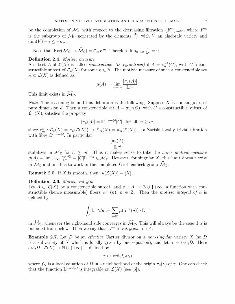
be the completion of MC with respect to the decreasing filtration Fmm∈Z, where Fm

is the subgroup of MC generated by the elements [V ]Li with V an algebraic variety and

dim(V )− i ≤ −m.

Note that Ker(MC → MC) = ∩mFm. Therefore limn→∞1

Ln = 0.

Definition 2.4. Motivic measureA subset A of L(X) is called constructible (or cylindrical) if A = π−1

n (C), with C a con-structible subset of Ln(X) for some n ∈ N. The motivic measure of such a constructible setA ⊂ L(X) is defined as:

µ(A) := limn→∞

[πn(A)]

Lnd.

This limit exists in MC.

Note. The reasoning behind this definition is the following. Suppose X is non-singular, ofpure dimension d. Then a constructible set A = π−1

m (C), with C a constructible subset ofLm(X), satisfies the property

[πn(A)] = L(n−m)d[C], for all n ≥ m,

since πnm : Ln(X) = πn(L(X)) → Lm(X) = πm(L(X)) is a Zariski locally trivial fibration

with fibre C(n−m)d. In particular[πn(A)]

Lnd

stabilizes in MC for n ≥ m. Thus it makes sense to take the naive motivic measureµ(A) = limn→∞

[πn(A)]Lnd = [C]L−md ∈ MC. However, for singular X, this limit doesn’t exist

inMC and one has to work in the completed Grothendieck group MC.

Remark 2.5. If X is smooth, then: µ(L(X)) = [X].

Definition 2.6. Motivic integralLet A ⊂ L(X) be a constructible subset, and α : A → Z ∪ +∞ a function with con-structible (hence measurable) fibers α−1(n), n ∈ Z. Then the motivic integral of α isdefined by ∫

A

L−αdµ :=∑n∈Z

µ(α−1(n)) · L−n

in MC, whenever the right-hand side converges in MC. This will always be the case if α isbounded from below. Then we say that L−α is integrable on A.

Example 2.7. Let D be an effective Cartier divisor on a non-singular variety X (so Dis a subvariety of X which is locally given by one equation), and let α = ordtD. HereordtD : L(X)→ N ∪ +∞ is defined by

γ 7→ ordtfD(γ)

where fD is a local equation of D in a neighborhood of the origin π0(γ) of γ. One can checkthat the function L−ordtD is integrable on L(X) (see [5]).

8 LAURENTIU MAXIM

Example 2.8. Let X = C1 and D be the divisor associated to the function xa, with a ∈ N,i.e., D is the origin 0 with multiplicity a. Let A be the set of arcs with the origin at0 ∈ C:

A = γ ∈ L(C1) | π0(γ) = γ(0) = 0 = π−10 (0).

By its definition, A is a constructible subset of L(C1), and it consists of all power series inthe variable t with zero constant term (i.e., of order at least 1). Our goal is to calculate:∫

A

L−ordtDdµ.

By definition, this equals ∑k≥0

µ(γ ∈ A | (ordtD)(γ) = k) · L−k

and note that (ordtD)(γ) = ordt(γa) has only values in positive multiples of a (since

ordt(γ) := n ≥ 1). Then the only values k ≥ 0 that appear in the sum are of the formk = na, with n ≥ 1. Therefore, by re-indexing, we can now write:∫

A

L−ordtDdµ =∑n≥1

µ(γ ∈ L(C1) | ordt(γ) = n) · L−na.

Next note that

πn(γ ∈ L(C1) | ordt(γ) = n) = an · tn | an 6= 0 = C \ 0.Hence, given that X is smooth, we have that

µ(γ ∈ L(C1) | ordt(γ) = n) =[C \ 0]

Ln=

L− 1

Ln.

We can now finish calculating our integral:

(2.1)

∫A

L−ordtDdµ =∑n≥1

(L− 1)

Ln· L−na = (L− 1) ·

∑n≥1

L−n(a+1) = (L− 1) · L−(a+1)

1− L−(a+1)

=L− 1

L(a+1) − 1=

1

1 + L + · · ·+ La=

1

[Pa].

If in the above example one considers the integral over the whole arc space L(C1), oneobtains similarly (the summation above starts at n = 0):∫

L(C1)

L−ordtDdµ =(L− 1)L(a+1)

L(a+1) − 1= (L− 1) +

L− 1

L(a+1) − 1.

The above example can be regarded as a motivation for the following very useful formula:

Proposition 2.9. ([5], Thm 2.15) Let X be non-singular and D =∑

i∈S aiDi an effec-tive simple normal crossing divisor (i.e., all Di are nonsingular hypersurfaces intersectingtransversally, and occurring with multiplicity ai). Denote D

I = (∩i∈IDi) \ (∪l /∈IDl) forI ⊂ S. The sets D

I form a locally closed stratification of X (with D∅ = X \Dred). Then∫

L(X)

L−ordtDdµ =∑I⊂S

[DI ]∏i∈I

L− 1

Lai+1 − 1=∑I⊂S

[DI ]∏

i∈I [Pai ].


The next result may be interpreted as a change of variable formula for the motivic integral.We will state the result in its simplest form, the one most frequently used in practice. Fora more general statement, we refer to [14], §3.8.

Proposition 2.10. ([5], Thm 2.18)Let h : Y → X be a proper birational morphism between smooth complex algebraic varieties,and let KY |X = KY − h∗KX be its discrepancy divisor 2. If D is an effective divisor on X,then

(2.2)

∫L(X)

L−ordtDdµ =

∫L(Y )

L−ordt(h∗D+KY |X)dµ.

Here h∗D is the pull-back of D, i.e. locally given by the equation f h, if D is locally givenby the equation f .

Remark 2.11. In the equality (2.2), one may replace L(X) by any constructible set A ⊂L(X), and L(Y ) by the preimage h−1(A) of A. More generally, one can replace ordtD byany function α : A → Z ∪ ∞ such that L−α is integrable on A (in which case ordt(h

∗D)will be replaced by α H, for H : L(Y )→ L(X) the map on the spaces of formal arcs thatis induced by h). In particular, in the setting of the above theorem, for a constructible setA ⊂ X we have:

µ(A) =

∫A

L0dµ(2.2)=

∫h−1(A)

L−ordtKY |X =∑n≥0

µL(Y )(γ ∈ h−1(A) | ordtJach(γ) = n) · L−n.

(recall here that KY |X is the effective divisor of the Jacobian determinant of h, since weassume that X and Y are smooth).

Remark 2.12. Let D be an effective divisor on a non-singular variety X. If D is a simplenormal crossing divisor, then we calculate the motivic integral

∫L(X)

L−ordtDdµ by using the

formula in Proposition 2.9. If D is not a simple normal crossing divisor, then we choose alog resolution of the pair (X,D), that is, a proper birational morphism h : Y → X froma non-singular variety Y , which is an isomorphism outside h−1(D) and such that h−1(D)is a divisor with strict normal crossings (i.e. the irreducible components of h−1(SuppD),denoted by Eii∈J , are smooth and intersect each other transversally). To the Ei’s thereare associated natural multiplicities ai and νi as follows: we set h∗D =

∑i∈J aiEi and

KY |X =∑

i∈J νiEi. Then the divisor h∗D + KY |X on Y is effective with simple normalcrossings, given by h∗D+KY |X =

∑i∈J(ai +νi)Ei. By the change of variables formula (2.2)

and the calculation from Proposition 2.9, we now obtain (with the obvious notations):∫L(X)

L−ordtDdµ =

∫L(Y )

L−ordt(h∗D+KY |X)dµ =∑I⊂J

[EI ]∏i∈I

L− 1

Lai+νi+1 − 1.

This formula can be regarded as a motivic integral associated to the pair (X, D).

3. Birational Calaby-Yau manifolds. K-equivalent varieties

This section deals with some of the first applications of motivic integration, which in factmotivated the development of the theory of motivic integration.

2since X and Y are smooth, KY |X is exactly the effective divisor of the Jacobian determinant of h.

10 LAURENTIU MAXIM

Definition 3.1. A Calabi-Yau manifold of dimension d is a non-singular complete (i.e.compact) complex algebraic variety M , which admits a nowhere vanishing regular differen-tial d-form ωM . Alternative formulations of this condition are that the first Chern class ofthe tangent bundle of M is zero, or that the canonical divisor KM of M is trivial. Recallthat the canonical divisor is the divisor of zeros and poles of a differential d-form.

Definition 3.2. Two non-singular complete algebraic varieties X and Y are called K-equivalent if there exists a non-singular complete algebraic variety Z and birational mor-phisms hX : Z → X an hY : Z → Y such that h∗XKX = h∗Y KY .

Proposition 3.3. If X and Y are birational equivalent Calabi-Yau manifolds or, more

generally, K-equivalent non-singular varieties then [X] = [Y ] in MC.

Proof. If X and Y are birationally equivalent there exist a non-singular complete algebraicvariety Z and birational morphisms hX : Z → X an hY : Z → Y . For K-equivalentmanifolds, these objects are part of the definition. Now, for X non-singular, and for Z andhX as above, if one denotes KZ|X := KZ − hX

∗(KX) then:

[X] = µ(L(X))(∗)=

∫L(X)

L0 dµ(∗∗)=

∫L(Z)

L−ordtKZ|Xdµ,

where (∗) follows by the definition of the motivic integral for α = 0, and (∗∗) is the changeof variable formula. For Calabi-Yau’s X and Y , we have that KZ|X = KZ|Y = KZ . ForK-equivalent manifolds, we also have KZ|X = KZ|Y . This finishes the proof.

Corollary 3.4. (Kontsevich) In particular, it follows that birationally equivalent Calabi-Yau manifolds or, more generally, K-equivalent manifolds, have the same E-polynomial,therefore they have the same Hodge numbers (hence the same Betti numbers).

Remark 3.5. Intermezzo on Birational Geometry.An irreducible complex projective variety X is called a minimal model if X is terminal(for a definition see §4) and KX is numerically effective (shortly, nef ), i.e. the intersectionnumber KX · C ≥ 0 for any irreducible curve C on X. The Minimal Model Program pre-dicts the existence of a minimal model in every birational equivalence class of non-negativeKodaira dimension. The conjecture is proved in dimension 2, where there exists a uniqueminimal model, which moreover is smooth. In dimension 3, a minimal model exists but itis not unique in a given birational equivalence class of non-negative Kodaira dimension. Indimensions ≥ 4, the Minimal Model Program is still a major conjecture in algebraic geom-etry. In [15], Wang showed that birationally equivalent minimal models, if they exist, areK-equivalent (see definition 8.6). Therefore, by the above corollary, birationally equivalentsmooth minimal models have the same Hodge numbers, hence the same Betti numbers.

Remark 3.6. Let h : Y → X be a proper birational morphism between non-singularalgebraic varieties. Assume that the exceptional locus of h, i.e. the subvariety of Y whereh is not an isomorphism, is a simple normal crossing divisor, and let Di, i ∈ S be itsirreducible components. The relative canonical divisor (i.e. the discrepancy divisor of h) issupported on the exceptional locus, and let νi − 1 be the multiplicity of Di in this divisor.So KY |X =

∑i∈S(νi−1)Di. Note that, since X and Y are non-singular, KY |X is an effective


divisor, more precisely it is locally defined by the ordinary Jacobian determinant with respectto local coordinates on X and Y . Denoting D

I = (∩i∈IDi) \ (∪l /∈IDl) for I ⊂ S, we have:

(3.1) [X] =∑I⊂S

[DI ]∏i∈I

L− 1

Lνi − 1=∑I⊂S

[DI ]∏i∈I

1

[Pνi−1]∈ MC

Indeed, since X is non-singular, by the change of variable formula we have:

[X] = µ(L(X)) =

∫L(X)

1 dµ =

∫L(Y )

L−ordtKY |Xdµ,

and Proposition 2.9 yields the above formula. Specializing to the topological Euler char-acteristic yields the following formula which motivates the definition of the stringy Eulernumber (see §4):

χ(X) =∑I⊂S

χ(DI )∏i∈I

1

νi

.

4. Stringy invariants

Stringy invariants are associated to certain singular spaces with mild singularities, andextend the classical corresponding topological invariants of smooth varieties. Stringy in-variants are defined in terms of data of log resolutions, however they are independent of allchoices involved.

Definition 4.1. Gorenstein conditionA complex algebraic variety X is called Q-Gorenstein if X is normal, irreducible (or puredimensional), and some multiple rKX (r ∈ N) of the canonical Weil divisor KX is a Cartierdivisor. The case r = 1 corresponds to a Gorenstein variety, e.g. if X is smooth. HereKX is the Zariski-closure of a canonical divisor on the regular part of X (it is well-definedby the normality assumption), or equivalently, the divisor of zeros and poles of a rationaldifferential d-form on X. With this, X is Gorenstein if the rational differential d-forms onX which are regular on Xreg are locally generated by one element.

Example 4.2. All normal hypersurfaces and complete intersections are Gorenstein.

Definition 4.3. Let X be a Gorenstein variety of dimension d and let h : Y → X be alog resolution of singularities of X, so the exceptional divisor D is a simple normal crossingdivisor. Denote by Di , i ∈ S, the irreducible components of the exceptional locus. SinceKX is a Cartier divisor, the pullback h∗KX makes sense. The discrepancy divisor of his Kh = KY |X := KY − h∗KX . h is called a crepant resolution/desingularization of X ifKh = 0.

The discrepancy divisor of h is supported on the exceptional locus, and we write

KY |X =∑i∈S

(ai − 1)Di.

We call ai the log discrepancy of Di with respect to X, and call ai−1 its discrepancy. The logdiscrepancies of a Q-Gorenstein variety are defined analogously by KY |X =

∑i∈S(ai− 1)Di,

which should be interpreted as rKY |X = rKY − h∗(rKX) =∑

i∈S r(ai − 1)Di.

12 LAURENTIU MAXIM

Note that, if X is Gorenstein then ai ∈ Z, and when X is non-singular ai ≥ 2, for alli ∈ S. For Q-Gorenstein varieties, we have that ai ∈ Q for all i ∈ S (more precisely,r(ai − 1) ∈ Z, so ai ∈ 1

rZ).

Definition 4.4. Let X be a Q-Gorenstein variety , and take a log resolution h : Y → X ofX with log discrepancies ai ∈ Q, i ∈ S. Then X is called

(1) terminal if ai > 1 for all i ∈ S;(2) canonical if ai ≥ 1 for all i ∈ S;(3) log terminal if ai > 0 for all i ∈ S;(4) log canonical if ai ≥ 0 for all i ∈ S;(5) strictly log canonical if it is log canonical but not log terminal.

Remark 4.5. Note that 0 is the relevant border value, since if some ai < 0 on somelog resolution, then one can construct log resolutions with arbitrarily negative ai. Thelog terminal singularities are considered as being mild ; the singularities which are not logcanonical are considered as general.

Proposition 4.6. Relation with arc spaces (Ein, Mustata, Yasuda)Let X be a normal variety which is locally a complete intersection. Then X is terminal,canonical and log canonical if and only if Ln(X) is normal, irreducible and equidimensional,resp., for all n.

For a log terminal algebraic variety X, one can define stringy invariants in terms of a logresolution of X.

Definition 4.7. Let X be a log terminal algebraic variety and h : Y → X a log resolu-tion. Let Di, i ∈ S be the irreducible components of the exceptional locus of h, with logdiscrepancies ai ∈ Q>0. Denote D

I = (∩i∈IDi) \ (∪l /∈IDl) for I ⊂ S.

(1) The stringy Euler number of X is:

χst(X) :=∑I⊂S

χ(DI )∏i∈I

1

ai

∈ Q.

(2) The stringy E-function of X is:

Est(X) = Est(X; u, v) :=∑I⊂S

E(DI )∏i∈I

uv − 1

(uv)ai − 1

and the stringy χy-genus of X is defined by

χsty (X) = Est(X;−y, 1).

(3) The stringy E-invariant of X is:

Est(X) :=∑I⊂S

[DI ]∏i∈I

L− 1

Lai − 1.

Note. From the above definition, we see that χst(X) = lim(u,v)→(1,1) Est(X). Note that wehave specialization maps Est 7→ Est 7→ χst. When X is nonsingular, we have Est(X) = [X](by (3.1)), and so Est(X) = E(X) and χst(X) = χ(X). Thus these are new singularityinvariants generalizing the invariants [·], E(·) and χ(·) resp., for X smooth.


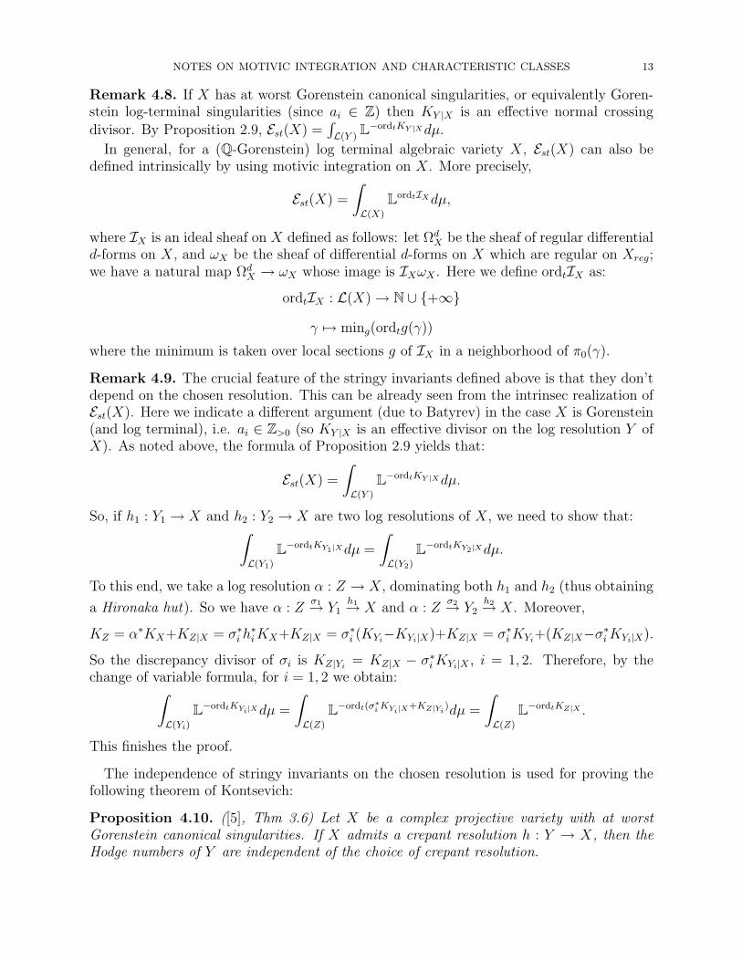
Remark 4.8. If X has at worst Gorenstein canonical singularities, or equivalently Goren-stein log-terminal singularities (since ai ∈ Z) then KY |X is an effective normal crossingdivisor. By Proposition 2.9, Est(X) =

∫L(Y )

L−ordtKY |Xdµ.

In general, for a (Q-Gorenstein) log terminal algebraic variety X, Est(X) can also bedefined intrinsically by using motivic integration on X. More precisely,

Est(X) =

∫L(X)

LordtIXdµ,

where IX is an ideal sheaf on X defined as follows: let ΩdX be the sheaf of regular differential

d-forms on X, and ωX be the sheaf of differential d-forms on X which are regular on Xreg;we have a natural map Ωd

X → ωX whose image is IXωX . Here we define ordtIX as:

ordtIX : L(X)→ N ∪ +∞

γ 7→ ming(ordtg(γ))

where the minimum is taken over local sections g of IX in a neighborhood of π0(γ).

Remark 4.9. The crucial feature of the stringy invariants defined above is that they don’tdepend on the chosen resolution. This can be already seen from the intrinsec realization ofEst(X). Here we indicate a different argument (due to Batyrev) in the case X is Gorenstein(and log terminal), i.e. ai ∈ Z>0 (so KY |X is an effective divisor on the log resolution Y ofX). As noted above, the formula of Proposition 2.9 yields that:

Est(X) =

∫L(Y )

L−ordtKY |Xdµ.

So, if h1 : Y1 → X and h2 : Y2 → X are two log resolutions of X, we need to show that:∫L(Y1)

L−ordtKY1|Xdµ =

∫L(Y2)

L−ordtKY2|Xdµ.

To this end, we take a log resolution α : Z → X, dominating both h1 and h2 (thus obtaining

a Hironaka hut). So we have α : Zσ1→ Y1

h1→ X and α : Zσ2→ Y2

h2→ X. Moreover,

KZ = α∗KX+KZ|X = σ∗i h∗i KX+KZ|X = σ∗i (KYi

−KYi|X)+KZ|X = σ∗i KYi+(KZ|X−σ∗i KYi|X).

So the discrepancy divisor of σi is KZ|Yi= KZ|X − σ∗i KYi|X , i = 1, 2. Therefore, by the

change of variable formula, for i = 1, 2 we obtain:∫L(Yi)

L−ordtKYi|Xdµ =

∫L(Z)

L−ordt(σ∗i KYi|X+KZ|Yi)dµ =

∫L(Z)

L−ordtKZ|X .

This finishes the proof.

The independence of stringy invariants on the chosen resolution is used for proving thefollowing theorem of Kontsevich:

Proposition 4.10. ([5], Thm 3.6) Let X be a complex projective variety with at worstGorenstein canonical singularities. If X admits a crepant resolution h : Y → X, then theHodge numbers of Y are independent of the choice of crepant resolution.

14 LAURENTIU MAXIM

Proof. The discrepancy divisor of a crepant resolution h : Y → X is zero by definition, soai = 1 for all i ∈ S. Therefore,

Est(X) =∑i∈S

E(DI ) = E(Y ).

On the other hand, the stringy E-function of X is independent of the chosen resolution;in particular, E(Y ) = Est(X) = E(Y ′), for any other crepant resolution h′ : Y ′ → X. Itremains to note that E(Y ) determines the Hodge-Deligne numbers of Y , and hence theHodge numbers since Y is smooth and projective.

5. Motivic volume

Definition 5.1. Motivic volumeIf X is a complex algebraic variety of pure dimension d, the motivic volume of X is themotivic measure of the whole arcspace of X, i.e. µ(L(X)). Recall the latter was defined by

µ(L(X)) = limn→∞

[πn(L(X))]

Lnd,

and it equals [X] when X is non-singular.

A formula for the motivic volume of X can be given in terms of a suitable resolution ofsingularities, by using Proposition 2.9 (see [14], §5.1).

Definition 5.2. arc-Euler characteristicLet Mloc be the subring of MC obtained from (the image of) MC by inverting all theelements [Pj], j ∈ N (since [Pj] = 1 + L + · · ·Lj, this is equivalent to inverting 1

Lj−1, j ∈ N).

As noted before, the E-polynomial and the Euler characteristic extend from MC to Mloc.The arc-Euler characteristic of a variety X is defined as χ(µ(L(X))), and it generalizes theusual Euler characteristic χ(X) for non-singular X.

6. Motivic zeta function. Monodromy conjecture

Let M be a non-singular irreducible variety of dimension m, and f : M → C a non-constant regular function. Let X := f = 0. For each n ∈ N, let fn : Ln(M) → Ln(C)be the morphism induced on the arc-space level by the morphism f . Any point δ ∈ Ln(C)corresponds to an element δ(t) ∈ C[t]/(tn+1); denote by ordtδ the largest k ∈ 1, .., n, +∞such that tk|δ(t). Set

Xn := γ ∈ Ln(M) | ordtfn(γ) = n, for n ∈ N.

Then Xn is a locally closed subvariety of Ln(M). Moreover, if n ≥ 1, then πn0 (Xn) ⊂ X.

Definition 6.1. The motivic zeta function of f : M → C is the formal power series:

Z(T ) :=∑n≥0

[Xn](L−mT )n

in MC[[T ]].


Remark 6.2. If D is the (effective) divisor of zeros of f , then:∫L(X)

L−ordtDdµ = Z(L−1).

The following result shows how to calculate the motivic zeta function Z(T ) in terms of aresolution:

Proposition 6.3. Let h : Y → M be an embedded resolution of f = 0, i.e. h is aproper birational morphism from a non-singular variety Y such that h is an isomorphismon Y \ h−1(f = 0), and h−1(f = 0) is a normal crossing divisor. Let Dii∈S be theirreducible components of h−1(f = 0), and set D

I = (∩i∈IDi) \ (∪l /∈IDl), for I ⊂ S. If weset div(f h) =

∑i∈S aiDi and Kh = KY |M =

∑i∈S(νi − 1)D1, then:

Z(T ) =∑I⊂S

[DI ]∏i∈I

(L− 1)T ai

Lνi − T ai.

In particular, Z(T ) is rational and belongs to the subring ofMC[[T ]] generated byMC andthe elements T a

Lν−T a , where ν, a ∈ Z>0.

Remark 6.4. The motivic zeta function Z(T ) specializes to the topological zeta function off . Indeed, evaluate Z(T ) at T = L−s, for any s ∈ N, and obtain the well-defined elements∑

I⊂S

[DI ]∏i∈I

L− 1

Lνi+sai − 1=∑I⊂S

[DI ]∏i∈I

1

[Pνi+sai−1]

inMloc. Applying the Euler characteristic χ(·) yields the rational numbers

(6.1)∑I⊂S

χ(DI )∏i∈I

1

νi + sai

for s ∈ N. The topological zeta function Ztop(s) of f is the unique rational function in onevariable s admitting the above values for s ∈ N. In particular, this specialization argumenttogether with the intrinsec definition of the motivic zeta function (based on the notion ofarc spaces) show that Ztop(s) does not depend on the chosen resolution h : Y → M (apriori, this fact is not clear at all, if one takes the equation (6.1) as the definition of thevalue Ztop(s)).

There is a conjectural relation between the poles of the topological zeta function and theeigenvalues of the local monodromy of f . This is know as the monodromy conjectureand asserts the following: If s0 is a pole of Ztop(s), then e2πis0 is an eigenvalue of the localmonodromy action on the cohomology of the Milnor fiber of f at some point of f = 0.One can formulate a motivic monodromy conjecture as follows: Z(T) belongs to the ringgenerated by MC and the elements T a

Lν−T a , where ν, a ∈ Z>0 and e2πi νa is an eigenvalue of

the local monodromy as above.

7. McKay Correspondence

One of the most striking application of motivic integration is Batyrev’s proof of theconjecture of Reid on the generalized McKay correspondence.

16 LAURENTIU MAXIM

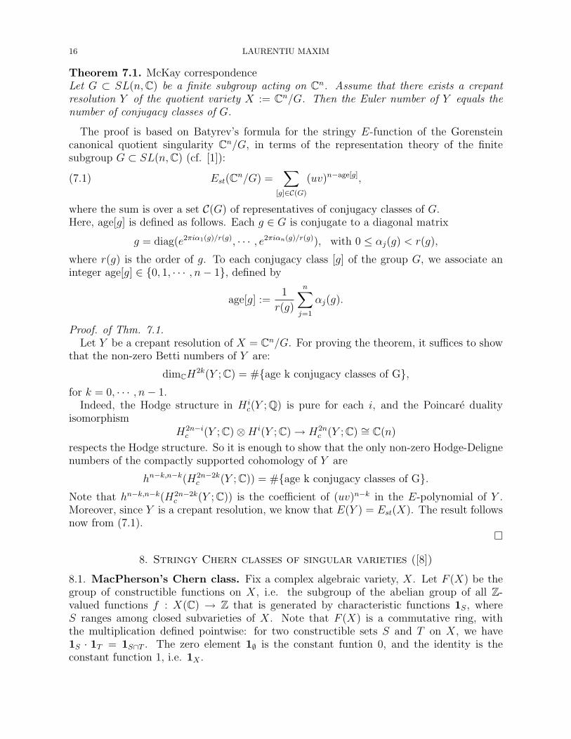
Theorem 7.1. McKay correspondenceLet G ⊂ SL(n, C) be a finite subgroup acting on Cn. Assume that there exists a crepantresolution Y of the quotient variety X := Cn/G. Then the Euler number of Y equals thenumber of conjugacy classes of G.

The proof is based on Batyrev’s formula for the stringy E-function of the Gorensteincanonical quotient singularity Cn/G, in terms of the representation theory of the finitesubgroup G ⊂ SL(n, C) (cf. [1]):

(7.1) Est(Cn/G) =∑

[g]∈C(G)

(uv)n−age[g],

where the sum is over a set C(G) of representatives of conjugacy classes of G.Here, age[g] is defined as follows. Each g ∈ G is conjugate to a diagonal matrix

g = diag(e2πiα1(g)/r(g), · · · , e2πiαn(g)/r(g)), with 0 ≤ αj(g) < r(g),

where r(g) is the order of g. To each conjugacy class [g] of the group G, we associate aninteger age[g] ∈ 0, 1, · · · , n− 1, defined by

age[g] :=1

r(g)

n∑j=1

αj(g).

Proof. of Thm. 7.1.Let Y be a crepant resolution of X = Cn/G. For proving the theorem, it suffices to show

that the non-zero Betti numbers of Y are:

dimCH2k(Y ; C) = #age k conjugacy classes of G,for k = 0, · · · , n− 1.

Indeed, the Hodge structure in H ic(Y ; Q) is pure for each i, and the Poincare duality

isomorphismH2n−i

c (Y ; C)⊗H i(Y ; C)→ H2nc (Y ; C) ∼= C(n)

respects the Hodge structure. So it is enough to show that the only non-zero Hodge-Delignenumbers of the compactly supported cohomology of Y are

hn−k,n−k(H2n−2kc (Y ; C)) = #age k conjugacy classes of G.

Note that hn−k,n−k(H2n−2kc (Y ; C)) is the coefficient of (uv)n−k in the E-polynomial of Y .

Moreover, since Y is a crepant resolution, we know that E(Y ) = Est(X). The result followsnow from (7.1).

8. Stringy Chern classes of singular varieties ([8])

8.1. MacPherson’s Chern class. Fix a complex algebraic variety, X. Let F (X) be thegroup of constructible functions on X, i.e. the subgroup of the abelian group of all Z-valued functions f : X(C) → Z that is generated by characteristic functions 1S, whereS ranges among closed subvarieties of X. Note that F (X) is a commutative ring, withthe multiplication defined pointwise: for two constructible sets S and T on X, we have1S · 1T = 1S∩T . The zero element 1∅ is the constant funtion 0, and the identity is theconstant function 1, i.e. 1X .


Associated to any morphism of varieties f : X → Y , there is a group homomorphism, thepushforward f∗ : F (X) → F (Y ) such that, for any constructible set S ⊂ X, the functionf∗1S is defined pointwise by setting

f∗1S(y) = χc(f−1(y) ∩ S), for any y ∈ Y.

In particular, if S is a subvariety of X and g = f |S, then f∗1S = g∗1S.On any variety X, the Chow group Ak(X) is defined to be the free abelian group on the

k-dimensional irreducible closed subvarieties of X, modulo the subgroup generated by thecycles of the form [div(f)], where f is a non-zero rational function on a (k + 1)-dimensionalsubvariety of X.

Given a complex variety X, MacPherson defined a homomorphism of additive groups

c : F (X)→ A∗(X)

such that, when X is smooth and pure dimensional, one has c(1X) = c(TX) ∩ [X], wherec(TX) is the total Chern class of X and [X] is the class representing X in A∗(X). Moreover,the transformation c commutes with pushforwards along proper morphisms. The totalChern class of a singular variety X is defined as

cSM(X) := c(1X).

As a consequence of the functoriality of MacPherson transformation, one has that∫X

cSM(X) = χ(X)

where the integral sign means to take the degree of the zero-dimensional piece of the termfollowing.

8.2. Stringy Chern classes.

8.2.1. Relative motivic ring and relative motivic integration ([12]). Fix a complex algebraicvariety X. Let V arX be the category of X-varieties, that is, integral, separated schemes

of finite type over X. Given an X-variety Vg→ X, denote by V the corresponding

class modulo isomorphisms over X. Set LX := A1X. Let K0(V arX) be the free Z-

module generated by the isomorphism classes of X-varieties, modulo the relation V =V \W+ W, for W a closed subvariety of an X-variety V (here both W and V \W areviewed as X-varieties under the restriction of the morphism V → X). K0(V arX) becomesa ring when the product is defined by setting V · W = V ×X W, and extending it

associatively. This ring has as zero element ∅, and the identity element X = X id→ X.We define

MX := K0(V arX)[L−1X ],

and still use the symbol V to denote the class of the X-variety V in MX . Completingwith respect to the dimensional filtration Fm

X (as m → ∞) we obtain the relative motivic

ring MX . Here FmX is the subgroup of MX generated by elements V · L−i

X , with V anX-variety such that dimC(V )− i ≤ −m. We denote by

τ = τX : K0(V arX)→ MX

the composition of maps K0(V arX)→MX → MX .

18 LAURENTIU MAXIM

All main definitions and properties valid for motivic integration over SpecC translate tothe relative setting by remembering the maps over X. For instance, let Y be a smoothX-variety, represented by a morphism f : Y → X. Let L(Y ) be the space of formal arcs onY , and denote by Cyl(L(Y )) the set of cylinders (i.e. constructible subsets) on L(Y ). Thenthe relative motivic (pre-)measure

µX : Cyl(L(Y ))→ MX

is defined as follows. For A ∈ Cyl(L(Y )), we choose an integer m such that π−1m (πm(A)) = A

(this is possible since Y is smooth, hence any cylinder is stable), and put

µX(A) := πm(A) · L−m·dimC(Y )X

where πm(A) is regarded as a constructible set over X under the composite morphismLm(Y )→ Y → X. This definition does not depend on the choice of m.

In order to define the relative motivic integral, consider an effective divisor D on Y ,together with the associated function ordtD : L(Y )→ N ∪ ∞. Its level set are cylinders(except the one at infinity, which will be declared to have zero measure). Then the relativemotivic integral is defined by

(8.1)

∫L(Y )

L−ordtDX dµX :=

∑n≥0

µX((ordtD)−1(n)

)· L−n

X .

This yields an element in MX .The change of variable formula also holds in the relative setting, more precisely:

Proposition 8.1. Let g : Y ′ → Y be a proper birational morphism between smooth varietiesover X, and let KY ′|Y be its discrepancy divisor. If D is an effective divisor on Y , then

(8.2)

∫L(Y )

L−ordtDX dµX =

∫L(Y ′)

L−ordt(g∗D+KY ′|Y )

X dµX .

The change of variables formula, together with Hironaka resolution of singularities, re-duces the computations to the case of a simple normal crossing effective divisor D =∑

i∈J aiEi on a smooth X-variety Y (here Ei are the irreducible components of SuppD).Then a calculation like in Proposition 2.9 yields the following:

(8.3)

∫L(Y )

L−ordtDX dµX =

∑I⊆J

EI∏

i∈IPaiX

,

where EI = (∩i∈IEi) \ (∪l /∈IEl) for I ⊂ J .

As a corollary of this formula, we obtain the important fact that every integral of theform (8.1) is an element in the image NX := Im(ρ) of the natural ring homomorphism

ρ : K0(V arX)[PaX−1]a∈N → MX .

8.2.2. Definition of stringy Chern classes. The crucial step in defining the stringy Chernclasses is to construct a ring homomorphism from a certain relative motivic ring to theQ-valued constructible functions on X. (Then compose with MacPherson’s Chern classtransformation in order to obtain the stringy Chern classes.) We will do this in few steps,starting with the case of an effective divisor on a smooth X-variety Y , then considering thecase when X itself is a Q-Gorenstein log-terminal variety. In the latter case, we choose a


log resolution of X, say Y , thus obtaining a pair of a smooth X-variety Y and a Q-Weildivisor, KY |X . This case requires more work, since we deal with Q-divisors, and we need toextend the motivic ring in order to be able to integrate order functions with rational values.

Case I. D is an effective divisor on a smooth X-variety Y .We begin by observing that if Y and Y ′ are X-varieties, then the fibers over x ∈ X satisfy:(Y ×X Y ′)x = Yx × Y ′

x. So we can define a ring homomorphism Φ0 : K0(V arX)→ F (X) bysetting

Φ0(Vg→ X) = g∗1V .

This is indeed a ring homomorphism since, by definition, for x ∈ X we have: g∗1V (x) =χc(g

−1(x)) = χc(Vx). Then for any x ∈ X: (Φ0(V · V ′)) (x) = χc((V ×X V ′)x) =χc(Vx × V ′

x) = χc(Vx) · χc(V′x) = (Φ0(V ) · Φ0(V ′))(x).

We proceed by extending Φ0 to a ring homomorphism Φ : NX → F (X)Q. In order todo this, first note that Φ0(Pa

X) = (a + 1)1X is an invertible element in F (X)Q, thus Φ0

extends uniquely to a ring homomorphism

Φ : K0(V arX)[PaX−1]a∈N → F (X)Q.

In order to get the desired extension to NX it suffices to observe that Φ kills the kernel of

ρ : K0(V arX)[PaX−1]a∈N → MX (cf. [8], (2.1)).

Now let D be an effective divisor on a smooth X-variety Y . Define

Φ(Y,D) = ΦX(Y,D) := Φ

(∫L(Y )

L−ordtDX dµX

)∈ F (X)Q.

When D = 0 write ΦXY , or just ΦY .

With the notations from the change of variable formula, i.e. for g : Y ′ → Y a birationalmorphism between smooth X-varieties (represented by morphisms f : Y → X and resp.f ′ : Y ′ → X) and D an effective divisor on Y , by applying Φ to both sides of formula (8.2)we obtain the following identity in F (X)Q:

Φ(Y,D) = Φ(Y ′,g∗D+KY ′|Y ).

Moreover, assuming that g∗D + KY ′|Y =∑

i∈J aiEi is a simple normal crossing divisor, byapplying Φ to formula (8.3) for the pair (Y ′, g∗D + KY ′|Y ) we obtain the following identityin F (X)Q:

(8.4) Φ(Y,D) = Φ(Y ′,g∗D+KY ′|Y ) =∑I⊆J

f ′∗1EI∏

i∈I(ai + 1)

In particular, if D = 0, then ΦY = Φ(Y ) = Φ0(Yf→ X) = f∗1Y .

Case II. X is a Q-Gorenstein log-terminal variety.In this case, we first choose a log resolution h : Y → X of X, i.e. the exceptional divisorh−1(Xsing) is a simple normal crossing divisor, and denote by Ei, i ∈ J the irreducible

20 LAURENTIU MAXIM

components of the exceptional locus. The discrepancy divisor KY |X is a Q-divisor, uniquelydefined by its discrepancies, i.e.

KY |X =∑i∈J

aiEi

with all ai ∈ Q and ai > −1 (this is the log-terminal condition). This should be interpretedas rKY |X = rKY − h∗(rKX) =

∑i∈J raiEi, for some r ∈ Z such that rai ∈ Z for every

i ∈ J .We would like to define a ring homomorphism Φ as in the previous case, and then an

element in F (X)Q, namely by setting

(8.5) ΦX := ΦX(Y,KY |X) = Φ

(∫L(Y )

L−ordtKY |XX dµX

).

Given that the divisor KY |X is now a Q-divisor, in order to make sense of this defin-ition we need to enlarge the motivic ring so that we can integrate order functions withrational values. We also need to adapt the definition of the ring homomorphism Φ to thisenlarged motivic ring. We will do this in what follows. But before that, notice that if Xis a Gorenstein canonical variety, then KY |X is an effective normal crossing divisor on thesmooth X-variety Y , and formula (8.5) makes sense from the considerations made in Case I.

Extending the relative motivic ring.Recall that by choosing a log resolution, we are in the following setting: Y is a smoothX-variety, and D =

∑i∈J aiEi is a simple normal crossing Q-divisor on Y , with ai > −1

for every i (here, D is the discrepancy divisor of our log resolution). Since Y is smooth, thisis equivalent to saying that (Y,−D) is a Kawamata log-terminal pair. Choose an integer r

such that rai ∈ Z for every i, and define the ring M1/rX to be the completion of

K0(V arX)[L±1/rX ]

with respect to a similar dimensional filtration as the one used in the case r = 1. Here L1/rX

is a formal variable with (L1/rX )r = LX , and we assign to it the dimension dimC(X) + 1

r.

Then we define

(8.6)∫L(Y )

L−ordtDX dµX notation

=

∫L(Y )

(L1/rX )−ordt(rD)dµX :=

∑n∈Z

µX((ordt(rD))−1(n)

)· (L1/r

X )−n.

In fact, an explicit computation shows that the summation is taken over N. This is thecrucial point in order to make sure that the sum in the right-hand side defines indeed an

element in M1/rX ; it is precisely at this point where we need the assumption of log-terminality.

In addition, a standard computation yields the following formula for the integral:

(8.7)

∫L(Y )

L−ordtDX dµX =

∑I⊆J

EI∏i∈I

∑r−1t=0 (L1/r

X )t∑r(ai+1)−1t=0 (L1/r

X )t.

This is just formula (8.3), with L regarded as (L1/r)r. From this formula we also see thatthe assumption ai > −1 is necessary indeed.


Extending the homomorphism Φ.

In view of the desired formula (8.5), we want to be able to extend Φ to M1/rX . More precisely,

by formula (8.7), it suffices to extend Φ to the smallest subring of M1/rX that contains the

values of the relative motivic integral. This subring will be denoted by N 1/rX .

We first extend the ring homomorphism Φ0 : K0(V arX)→ F (X) to a ring homomorphism

Φ0 : K0(V arX)[L1/rX ]→ F (X)

by setting Φ0(L1/rX ) = 1X . Observing that Φ0(

∑bt=0(L

1/rX )t) = (b + 1)1X , conclude as in

Case I that Φ0 induces a ring homomorphism

Φ : N 1/rX → F (X)Q.

Also note that for every rational number a > −1 and any choice of r ∈ Z such that ra ∈ Z,we have:

Φ

( ∑r−1t=0 (L1/r

X )t∑r(a+1)−1t=0 (L1/r

X )t

)=

r

r(a + 1)1X =

1X

a + 1,

which, in particular, does not depend on the choice of r. Therefore, formula (8.5) makesnow complete sense:

ΦX := ΦX(Y,KY |X) = Φ

(∫L(Y )

L−ordtKY |XX dµX

).

This definition is independent of the choice of resolution since any two resolutions aredominated by a third, and it is enough to observe the following:

Proposition 8.2. ([8], Prop. 3.2) Let Y be a smooth X-variety, and D be a simple normalcrossing divisor on Y such that (Y,−D) is a log-terminal pair. Let g : Y ′ → Y be a properbirational morphism such that Y ′ is smooth and KY ′|Y + g∗D is a simple normal crossingdivisor. Then (Y ′,−(KY ′|Y + g∗D)) is a log-terminal pair, and

ΦX(Y,D) = ΦX

(Y ′,KY ′|Y +g∗D).

Now if D = KY |X is the discrepancy divisor of the log resolution Y of X, the aboveidentity turns into ΦX

(Y,KY |X) = ΦX(Y ′,KY ′|X), by noting that KY ′|X = KY ′|Y + g∗KY |X .

Formula (8.4) from Case I still holds in this more general setting by allowing ai to berational numbers larger than −1.

We have now all the ingredients for defining the stringy Chern classes.

Definition 8.3. Let X be a Q-Gorenstein log-terminal variety. The stringy Chern class ofX is the class

cst(X) := c(ΦX) ∈ A∗(X)Q,

where c : F (X)Q → A∗(X)Q is MacPherson’s Chern class transformation, tensored with Q.

22 LAURENTIU MAXIM

8.2.3. Properties of stringy Chern classes.

Proposition 8.4. Let X be a proper Q-Gorenstein log-terminal variety. Then∫X

cst(X) = χst(X).

Proof. Let h : Y → X be a log resolution of singularities for X, and let Ei, i ∈ J , denote theirreducible components of the exceptional locus. Then KY |X =

∑i kiEi is a simple normal

crossing Q-divisor. By formula (8.4), adapted to the case of log-terminal pairs, and usingthe properness of h, we have:

cst(X) = c(ΦX) = c(ΦX(Y,KY |X)) = c

(∑I⊆J

h∗1EI∏

i∈I(ki + 1)

)= h∗c

(∑I⊆J

1EI∏

i∈I(ki + 1)

)Since the clossure of each stratum of the stratification X = tI⊆JE

I is a union of strata,there exist rational numbers bI such that:∑

I⊆J

1EI∏

i∈I(ki + 1)=∑I⊆J

bI1EI.

Therefore,∫X

cst(X) =

∫Y

∑I⊆J

bIcSM(EI ) =

∑I⊆J

bI

∫E

I

cSM(EI ) =

∑I⊆J

bIχ(EI ) =

∑I⊆J

χ(EI )∏

i∈I(ki + 1)= χst(X).

Proposition 8.5. If X admits a crepant resolution h : Y → X, then

cst(X) = h∗(c(TY ) ∩ [Y ]).

In particular, if X is smooth, then cst(X) = c(TX) ∩ [X].

Proof. Since KY |X = 0, h is proper and Y is smooth, we have

cst(X) = c(ΦX) = c(ΦXY ) = c(h∗1Y) = h∗c(1Y) = h∗(c(TY ) ∩ [Y ]).

For the next result, we need the following extension of the definition of K-equivalence.

Definition 8.6. Two normal Q-Gorenstein varieties X and X ′ are said to be K-equivalentif there exists a smooth variety Y and proper birational morphisms f : Y → X and f ′ :Y → X ′ such that KY |X = KY |X′ .

If X and X ′ are K-equivalent varieties, then the condition on the relative canonicaldivisors is satisfied for every choice of Y , f and f ′.

Theorem 8.7. Let X and X ′ be Q-Gorenstein log-terminal varieties, and assume that they

are K-equivalent. Consider any diagram Xf← Y

f ′→ X ′ with Y a smooth variety and f andf ′ proper birational morphisms. Then:

(1) There is a class C ∈ A∗(Y )Q such that f∗(C) = cst(X) in A∗(X)Q and f ′∗(C) =cst(X

′) in A∗(X′)Q.


(2) Assume that K := KY |X = KY |X′ is a simple normal crossing divisor∑

i∈J kiEi.Then

C = c

(∑I⊆J

1EI∏

i∈I(ki + 1)

).

Proof. It suffices to prove the theorem under the assumption that K is simple normal cross-ing divisor. Indeed, by further blowing up Y , we can always reduce to this case, and notethat push-forward on Chow groups is functorial for proper morphisms. Then, defining C asin the second part of the statement, we have:

f∗(C) = c

(∑I⊆J

f∗1EI∏

i∈I(ki + 1)

)= c(ΦX

(Y,K)) = c(ΦX) = cst(X),

and similarly f ′∗(C) = cst(X′).

8.3. McKay correspondence for stringy Chern classes. Here we survey [8] §6, wherethe authors compare the stringy Chern classes of quotient varieties with Chern-Schwartz-MacPherson classes of fixed point-set data.

Let M be a smooth quasi-projective complex variety, and let G be a finite group withan action on M such that the canonical line bundle on M descends to the quotient (theexample that should be kept in mind is that of a finite subgroup of SL(n, C) acting onCn). Let X := M/G, with projection π : M → X. Then X is normal and has Gorensteincanonical singularities.

There are two ways of breaking the orbifold X into simpler pieces. (1.) The first wayis to stratify X according to the stabilizers of the points on M . For any subgroup H ofG, let XH ⊆ X be the set of points x such that for every y ∈ π−1(x) the stabilizer of y,Gy = g ∈ G : gy = y, is conjugate to H. If we let H run in a set S(G) of representativesof conjugacy classes of subgroups of G, obtain a stratification of X as

X = tH∈S(G)XH .

(2.) The second way is to look at fixed-point sets as orbifolds under the action of thecorresponding centralizers. For every g ∈ G, consider the fixed-point set M g = x ∈ M :gx = x. The centralizer of g, defined as C(g) = h ∈ G : gh = hg, acts on M g and thereis a commutative diagram:

M g

// M

M g/C(g)

πg // X

Moreover M g/C(g), as an element in K0(V arX), is independent of the representative gchosen for its conjugacy class. Also note that πg is a proper morphism.

Fix a set C(G) of representatives of conjugacy classes of elements of G.

Theorem 8.8. With the above assumptions and notations, ΦX is an element in F (X) andthe following identities hold in F (X):

(8.8) ΦX =∑

H∈S(G)

|C(H)| · 1XH =∑

g∈C(G)

(πg)∗1Mg/C(g).

24 LAURENTIU MAXIM

The first equality follows from the motivic McKay correspondence. For the second equal-ity, the language of stacks is used.

As a corollary, we obtain a McKay correspondence for the stringy Chern classes. Moreprecisely:

Theorem 8.9.

(8.9) cst(X) =∑

g∈C(G)

(πg)∗cSM(M g/C(g)) ∈ A∗(X)

Proof. This follows by applying the transformation c : F (X)→ A∗(X) to the first and lastmembers of formula (8.8):

cst(X) =∑

g∈C(G)

c((πg)∗1Mg/C(g)) =∑

g∈C(G)

(πg)∗(c(1Mg/C(g))) =∑

g∈C(G)

(πg)∗cSM(M g/C(g)).

Definition 8.10. The orbifold Euler number of the quotient variety X = M/G is definedas

e(M, G) :=∑

g∈C(G)

χ(M g/C(g)).

Batyrev proved the following theorem:

Theorem 8.11. With the notations from the beginning of this section:

χst(X) = e(M, G).

When X is proper, this result follows from Proposition 8.4 and Theorem 8.9.

Remark 8.12. The construction of stringy Chern classes, that makes the object of thissection, has been greatly generalized to stringy classes T st

y whose associated genus is thestringy χy-genus, χst

y ([13]). The objects of this section are obtained by the substitutiony = −1. If X is smooth then T st

y (X) = T ∗y ∩ [X], where T ∗

y is the modified Todd class thatappears in the generalized Riemann-Roch theorem.

9. Singular Elliptic genus ([3])

This is an attempt to understand the work of Borisov and Libgober on generalizations ofelliptic genera to singular varieties.

9.1. Elliptic genera of complex manifolds. In this section X is a compact (almost)complex manifold of complex dimension d. Denote by TX its holomorphic tangent bundle.Let xll be the Chern roots of TX , i.e. the total Chern class of TX is formally factorizedas c(TX) =

∏l(1 + xl). Then the elliptic genus of X, denoted by Ell(X; y, q), is the genus

corresponding to the power series

Q(x) = xθ( x

2πi− z, τ)

θ( x2πi

, τ),


where q = e2πiτ , y = e2πiz, for z ∈ C and τ ∈ H. Here H is the upper-half plane and θ isthe Jacobi theta function, which is defined as

θ(z, τ) = q18 (2 sin πz)

∞∏l=1

(1− ql)∞∏l=1

(1− qly)(1− qly−1).

In short,

(9.1) Ell(X; y, q) =

∫X

∏l

xl

θ( xl

2πi− z, τ)

θ( xl

2πi, τ)

.

Note that the defining series Q(x) is not normalized, i.e.

Q(0) =1

2πi· θ(−z, τ)

θ′(0, τ)6= 1.

The normalized version of the elliptic genus is

Ell(X; y, q) =

∫X

∏l

xl

2πi·θ( xl

2πi− z, τ)θ′(0, τ)

θ( xl

2πi, τ)θ(−z, τ)

.

When q → 0, the elliptic genus is ’almost’ the Hirzebruch χy-genus. More precisely:

limq→0

Ell(X; y, q) = y−d/2χ−y(X),

whereχy(X) =

∑p,q

(−1)qhp,q(X)yp.

It follows thatEll(X; y = 1, q → 0) = χ−1(X) = χ(X)

is the topological Euler characteristic of the compact complex manifold X. And also

(−1)d/2Ell(X; y = −1, q → 0) = χ1(X) = σ(X)

is the signature of X.As it can be seen from (9.1), elliptic genus is a combination of the Chern numbers of X.

However, it turns out that it cannot be expressed via the Hodge numbers of X. Since itdepends only on the Chern numbers, the elliptic genus is a cobordism invariant.

By making use of elliptic genera, Gritsenko ([10]) proved the following interesting result:

Proposition 9.1. Let M be an almost complex manifold of complex dimension d such thatc1(M) = 0 in H2(M ; R). Then

d · χ(M) ≡ 0 mod 24.

Moreover, if c1(M) = 0 in H2(M ; Z), the stronger result holds

χ(M) ≡ 0 mod 8 if d ≡ 2 mod 8.

9.2. Elliptic genera of log-terminal varieties. In this section, we follow [3] and de-fine singular elliptic genera for projective Q-Gorenstein varieties with at worst log-terminalsingularities. Singular elliptic genera can be defined in a similar manner for Kawamatalog-terminal pairs, but in order to keep things simple, in this section we only present theQ-Gorenstein log-terminal case (but see also Remark 9.3).

26 LAURENTIU MAXIM

9.2.1. Definition.

Definition 9.2. Let X be a projective Q-Gorenstein variety with log-terminal singularities.Let h : Y → X be a log resolution of X, i.e. the exceptional divisor D =

∑k Dk is a simple

normal crossing divisor. The discrepancies ak of the components Dk of D are determinedby the relative canonical divisor of h, i.e.

KY = h∗KX +∑

k

akDk,

and the log-terminal condition translates into ak > −1 for all k. Let c(TY ) =∏

l(1 + yl),with yll the Chern roots of TY . Let ek = c1(Dk). The singular elliptic genus of X isdefined as a function of two variables y = e2πiz and q = e2πiτ by the following formula:

(9.2)

EllY (X; y, q) =

∫Y

(∏l

yl

2πi·θ( yl

2πi− z, τ)θ′(0, τ)

θ( yl

2πi, τ)θ(−z, τ)

)×

(∏k

θ( ek

2πi− (ak + 1)z, τ)θ(−z, τ)

θ( ek

2πi− z, τ)θ(−(ak + 1)z, τ)

).

Remark 9.3. The very same formula can be used to define singular elliptic genera asso-ciated to projective Kawamata log-terminal pairs (cf. [3], Def. 3.3). A Kawamata log-terminal pair (X, T ) consists of a normal variety X together with a Q-Weil divisor T suchthat KX + T is Q-Cartier. Then a log resolution of the pair (X, T ) is a proper birationalmorphism h : Y → X from a non-singular variety Y , such that D := h−1(Xsing ∪ T ) is anormal crossing divisor. The discrepancies ak of the components Dk of D are determinedby the formula

KY = h∗(KX + T ) +∑

k

akDk,

and the requirement that the discrepancy of the proper transform of a component of T isthe negative of the coefficient of T at that component. The log-terminal condition requiresthat ak > −1 for all k.

As expected, the definition does not depend on the choice of the desingularization Y ofX.

Theorem 9.4. The elliptic genus EllY (X; y, q) of a projective Q-Gorenstein log-terminalvariety X does not depend on the choice of the log resolution Y , so it defines an invariant

of X, simply denoted by Ell(X; y, q).

The proof uses the deep Weak Factorization Theorem. It suffices to show that

EllY (X; y, q) = EllY (X; y, q),

where Y is obtained from Y by a blow-up along a nonsingular variety Z. It also can beassumed that Z has normal crossings with the components Dk of the exceptional divisor ofthe log resolution h. For details, see [3].

9.2.2. Main Properties.

Proposition 9.5. The elliptic genera of two different crepant resolutions of a Gorensteinprojective variety coincide.


Proof. It suffices to show that the elliptic genus of a crepant resolution Y of a Gorensteinvariety X equals the singular elliptic genus of X. If the exceptional set of the crepantresolution h : Y → X is the simple normal crossing divisor D =

∑k Dk, then the second

term of the product in the definition of the singular elliptic genus of X is equal to 1, sinceall discrepancies ak are equal to 0. Thus, we have the desired equality

Ell(Y ; y, q) = Ell(X; y, q).

If the exceptional divisor is not a simple normal crossing divisor, one can further blow-upthe crepant resolution Y , to get a proper birational morphism g : Z → Y such that theexceptional divisor of g and that of f g are simple normal crossing divisors. Then thesingular elliptic genera of Y and X calculated via Z are given by the same formula sincethe discrepancies involved coincide. Indeed, we have KZ|X = g∗KY |X + KZ|Y = KZ|Y .

In relation with the stringy E-function of Batyrev, we have the following:

Proposition 9.6.

limq→0

Ell(X; y, q) = (y−12 − y

12 )dEst(X; y, 1) = (y−

12 − y

12 )dχst

−y(X).

As an addition to Batyrev’s result on the equality of Hodge numbers of birationallyequivalent Calabi-Yau manifolds, one can prove the following:

Proposition 9.7. The elliptic genera of two birational equivalent Calabi-Yau manifoldscoincide.

Proof. If X and Y are birationally equivalent there exists a non-singular complete algebraicvariety Z and birational morphisms hX : Z → X an hY : Z → Y . By further blowing-up, wecan assume that the exceptional divisors of hX and hY are simple normal crossing divisors.Moreover, the Calabi-Yau condition on X and Y implies that the discrepancy divisors ofhX and hY coincide: KZ|X = KZ = KZ|Y . Therefore the elliptic genera of X and resp. Yare calculated on Z using the same discrepancies, so they coincide.

9.3. McKay correspondence for elliptic genera ([4]). In this section we present thedefinition of the orbifold elliptic genus of a global quotient variety, and state a very generalform of McKay correspondence.

Definition 9.8. Let X be a smooth algebraic variety, acted upon by a finite group G. For apair of commuting elements g, h ∈ G, let Xg,h be a connected component of the fixed pointset of both g and h. Let TX |Xg,h = ⊕Vλ be the decomposition of the restriction to Xg,h ofthe tangent bundle into direct sum of bundles on which g (resp. h) acts by multiplicationby e2πiλ(g) (resp. e2πiλ(h)), for λ(g), λ(h) ∈ Q ∩ [0, 1). Denote by xλ the Chern roots of thebundle Vλ. Then the orbifold elliptic genus of X/G is defined by the following formula:(9.3)

Ellorb(X, G; z, τ) =1

|G|∑

gh=hg

∏λ(g)=λ(h)=0

xλ

∏λ

θ( xλ

2πi+ λ(g)− τλ(h)− z)

θ( xλ

2πi+ λ(g)− τλ(h))

e2πiλ(h)z[Xg,h].

28 LAURENTIU MAXIM

In order to formulate the McKay correspondence for elliptic genera, let X be a nonsingularprojective variety on which G acts effectively by biholomorphic transformations. Let µ :X → X/G be the quotient map, D =

∑i(νi − 1)Di be the ramification divisor, and let

∆X/G :=∑

j

(νj − 1

νj

)µ(Dj).

Theorem 9.9.

Ellorb(X, G; z, τ) =

(2πiθ(−z, τ)

θ′(0, τ)

)d

Ell(X/G, ∆X/G; y, q)

where Ell(X/G, ∆X/G; y, q) is the singular elliptic genus of the pair, as defined in Remark9.3.

Remark 9.10. By the ramification formula, it follows that µ∗(KX/G+∆X/G) = µ∗(KX/G)+D = KX . Moreover, (X/G, ∆X/G) is Kawamata log terminal ([1], Prop. 7.1).

References

[1] Batyrev, V., Non-Archimedian integrals and stringy Euler numbers of log terminal pairs, J. Eur. Math.Soc. 1, p. 5-33, 1999.

[2] Blickle, M., A short course on geometric motivic integration, math. AG/0507404.[3] Borisov, L., Libgober, A., Elliptic genera of singular varieties, Duke Math. Journal, 116 (2), p. 319-351,

2003.[4] Borisov, L., Libgober, A., McKay correspondence for elliptic genera, Annals of Math. 161, p.1521-1569,

2005.[5] Craw, A., An introduction to motivic integration, Strings and geometry, p. 203-225, Clay Math. Proc.,

3, Amer. Math. Soc., Providence, RI, 2004.[6] Danilov, V. I., Khovanskii, A. G., Newton polyhedra and an algorithm for computing Hodge-Deligne

numbers, Bull. AMS, Volume 30, no 1, 1994, 62-69.[7] Denef, J., Loeser, F., Geometry on arc spaces of algebraic varieties, European Congress of Mathematics,

Vol. I (Barcelona, 2000), 327-348, Progr. Math., 201, Birkhuser, Basel, 2001.[8] de Fernex, T., Lupercio, E., Nevins, T., Uribe, B., Stringy Chern classes of singular varieties,

math.AG/0407314.[9] Fulton, W., Introduction to toric varieties, Annals of Math. Studies 131, Princeton University Press,

1993.[10] Gritsenko, Elliptic genus of Calaby-Yau manifolds and Jacobi and Siegel modular forms, Algebra i

Analiz 11:5, 1999.[11] Hirzebruch, F., Topological methods in algebraic geometry, Springer, 1966[12] Looijenga, E., Motivic measures, Seminaire Bourbaki, Vol. 1999/2000, Asterisque, p. 267-297.[13] Schurmann, J., Yokura, S., A survey of characteristic classes of singular spaces, math.AG/0511175.[14] Veys, W., Arc spaces, motivic integration and stringy invariants, math.AG/0401374.[15] Wang, C. L., On the topology of birational minimal models, J. Diff. Geom. 50 (1998), 129-146.

L. Maxim : Department of Mathematics, University of Illinois at Chicago, 851 S MorganStreet, Chicago, Illinois, 60607, USA.

E-mail address: [email protected]

notes on motivic integration and characteristic classes …maxim/motivic.pdf · notes on motivic...

Documents