notes on mathematical problems on the dynamics of ...jabin/particlesinfluid3.pdf36 chapter 1....

36 CHAPTER 1. DYNAMICS OF PARTICLES IN A FLUID

Notes on Mathematical Problems on the

Dynamics of

Dispersed Particles interacting through a Fluid

P.E. Jabin (∗) and B. Perthame (∗)(∗∗)(∗) Ecole Normale Superieure, DMI

45, rue d’Ulm

75230 Paris Cedex 05, France

(∗∗) INRIA-Rocquencourt, Projet M3N

BP 105

78153 Le Chesnay Cedex, France

1 Introduction

In this Chapter, we present some mathematical problems related to the dy-namics of particles interacting through a fluid. We are interested in the dilutecases. We mean the cases where a transport Partial Differential Equations inthe phase space can be expected for the particles density. In order to derivethese transport equations explicitely, some assumptions on the fluid dynam-ics are necessary. They limit the validity of the model but still representsmany possible applications. Namely we assume that the fluid dynamics canbe reduced to two simple situations. The first situation is the simple case of apotential flow (perfect incompressible and irrotational flow). This is relevantto describe for instance the motion of bubbles in water (see G.K. Batchelor[2]) and focuses mainly on the added mass effect which means that to acce-larate bubbles requires to accelerate some part of the water too. The secondsituation is the more standard case of particles in a Stokes flow, for whichthe domains of application are suspensions or sedimendation.

1. INTRODUCTION 37

The case of a potential flow around the particles, leads to a difficulty inestablishing the equation for the particle density. A mathematical formalismwas developed by G. Russo and P. Smereka [26] which we will present here,in the improved version of H. Herrero, B. Lucquin and B. Perthame [19].We will recall here how one can derive, from the interacting system of par-ticles, a Vlasov type of equation for the particle density in the phase spaceg(t, x, p), here t ≥ 0 is the time, x ∈ IR3 represents the space position andp ∈ IR3 represents the total impulsion of particles (dual of the velocity in theLagrangian - Hamiltonian duality). This equation is

∂∂t

g + gradpH · gradxg − gradxH · gradpg = 0, (1.1)

H(t, x, p) = 12|p + Φ(t, x)|2, (1.2)

Φ(t, x) = λ B ∗ (P + ρΦ)(t, .).

Here B = B(x) is a given 3 × 3 matrix, λ is the kinetic parameter (relatingthe radius of the particles to the densities of the particles and of the fluid)and the macroscopic density and implusion ρ, P are defined by

ρ(t, x) =∫

IR3 g(t, x, p)dp, (1.3)

P(t, x) =∫

IR3 p g(t, x, p)dp. (1.4)

The difficulty to establish this equation, comes from the Lagrangian aspect

of the natural dynamics for the particles. It turns out that the Hamiltonianvariables are better adapted to mathematical manipulations and to mechan-ical interpretation (notice that the Hamiltonian variable is just the totalimpulsion of particles). But the derivation of the mean field equation (1.1)-(1.3) for the particles density is easier in Lagrangian variables. Then, oneissue is to understand how to define, in the kinetic P.D.E., the Lagrangianand Hamiltonian variables (and to understand also change of variables).

The second situation consists in considering a Stokes flow around the par-ticles. It leads to quite different mathematical issues. In order to establishequations for the particle density one can follow the same derivation as be-fore. From the full dynamics of particles - N body interaction - a first (andrestrictive) assumption is to make a dipole approximation for the fluid equa-tion. This reduces the dynamics to two-body interactions and thus allows


to settle the kinetic equation for the particle density f(t, x, v), here v is thevelocity of the particle. One obtains a Vlasov type equation.

∂∂t

f + v · gradxf + λdivv((κg + µA ?x j − v)f) = 0, (1.5)

j(t, x) =∫

IR3 v f(t, x, v)dv. (1.6)

The matrix A(x) is now related to the Stokes Equation, as well as B, inthe potential case, is related to the Laplace Equation. Also, g denotes thegravity vector, λ the kinetic parameter and µ = 3

4Na, with N the number

of particles, a their radius. Even though there is no mathematical difficultyin establishing this system, several mathematical questions arise concerning,for instance, various asymptotic behaviors (large time behavior cf [21], λvanishing...etc) They arise because the friction term plays a major role inthe particles dynamics for a Stokes flow. A particularly interesting situationis the limit λ → ∞. It gives an example of a macroscopic limit which is notobtained by the collisional process, but by a strong force term. In the caseat hand, it is proved in P.E. Jabin [22] that the macroscopic limit gives riseto the equation

∂∂t

ρ + div(ρ u) = 0, (1.7)

µA ?x (ρu) − u = g. (1.8)

The topic of these notes represent particular examples of a very activefield of fluid mechanics where kinetic physics plays a fundamental role. Usu-ally it is used in the derivation of models for particular situations, but also ofeffective equations for the motion. In no way we can give a complete accountof the literature in this domain and we prefer to refer to some general works.Concerning bubbly-potential flows, the paper by Y. Yurkovetsky and J.F.Brady [32] contains numerous recent references as well as considerations onstatistical physics aspects of the model and the effect of collisisons. For thiseffect, see also G. Russo and P. Smereka [27], J.F. Bourgat et al [6]. Thederivation of pde models and the use of kinetic description is a rather recentsubject, confer H.F. Bulthuis, A. Prosperetti and A.S. Sangani [7], A.S. San-gani and A.K. Didwana [28], P. Smereka [30] and the references therein. Onthe other hand, the dynamics of particles in a Stokes flow have lead to verynumerous works. Let us quote some of them : G.K. Batchelor and C.S. Wen

2. DYNAMICS OF BALLS IN A POTENTIAL FLOW 39

[8], F. Feuillebois [12], E.J. Hinch [16], R. Herczynski and I. Pienkowska [20]and the book by J. Happel and H. Brenner [17]. Other regimes have alsobeen studied and lead to mathematical models which have been analyzed forinstance by K. Hamdache [18] for the case of a more general incompressibleflow (and small particles), by D. Benedetto, E. Caglioti and M. Pulvirenti[3] for granular flow. Complex numerical simulations have been performedby B. Maury and R. Glowinski [25], R. Glowinski, T.W. Pan and J. Periaux[15], for high concentrations of particles (see also the references therein).

The outline of this Chapter is as follows. The next two sections aredevoted to the case of a potential flow ; in section 2 we derive the modeldynamical system and section 3 is devoted to the mean field equation. In thefourth section, we derive the dynamical system for the case of Stokes flow.The macroscopic limit is explained in Section 5. Some numerical tests forthe potential flow case are presented in the Appendix.

The sections are largely independant of each other. Except some nota-tions which are refered to in the text, they can be read independently.

2 Dynamics of Balls in a Potential Flow

In this Section, we consider the dynamics of N balls of radius a, interactingthrough a potential fluid. The motion of each ball modifies the global flowand thus produces a force on the other balls. Even though we consider thevery simplified situation of the dipole approximation of a potential flow, theresult is a complex dynamics. Here, we describe (under the assumption ofdiluted particles), the limiting behavior, as N → ∞ and a vanishes, of theparticles density. As we will see in Section II, as long as collisions betweenparticles are neglected and a specific relation holds between a and N , thisleads to the equation (1.1)-(1.3) for the distribution of particles in the phasespace (time, space and total impulsion).

Our notations are as follows. We consider N particles which centers aredenoted Xi(t), they move with velocities Vi(t). Here, t denotes the time and1 ≤ i ≤ N . These particles are balls of radius a, centered at Xi(t), they aredenoted Bi(t). The inward normal on the sphere ∂Bi(t) will be denoted byni(x). We also denote by ρf the fluid density and by ρp the particle density,their mass is thus mp = 4

3πa3ρp, another remarquable quantity which arises


later is the virtual mass of the fluid mv = 23πa3ρf . As we will see, there is

a fundamental number which decides of the validity of a dilute regime, it isgiven by

λ = 6πNa3 ρf

ρf + 2ρp(2.1)

This ratio has to be kept constant in the limit N → ∞. Finally, we use cal-graphic letters for the 3N dimensional vectors (or matrices acting on thesevectors). For instance XN = (X1, . . . , XN).

2.1 the full dynamics

The fluid around the particles is assumed to be given by the potential equa-tions. In other words, the fluid velocity v(t, x) is obtained as

v(t, x) = ∇φ(t, x), (2.2)

where the potential φ is just given by

∆φ(t, x) = 0 in IR3 −⋃N

i=1 Bi(t),∂φ∂ni

= Vi(t) · ni on ∂Bi(t).(2.3)

We implicity consider that the fluid is at rest at infinity, i.e. v vanishes atinfinity. From this potential φ, we can compute the pressure thanks to theBernouilli relation

p(t, x) = −ρf (∂φ

∂t+

|∇φ|2

2) . (2.4)

This makes v(t, x) a solution of the incompressible Euler Equations. Thedynamics of the particles is therefore defined by the fundamental principleof dynamics,

Xi(t) = Vi(t) ,

mpVi(t) = Fi(t) =∫

∂Bi(t)p(t, x)nidS .

(2.5)

Let us point out that the force Fi depends upon all the positions Xi(t) andvelocities Vi(t) of the particles, and also of their derivatives. Especially Fi

depends upon ddt

Vi(t). This shows that this dynamics is rather complex andis not explicitely solvable by the Cauchy-Lipschitz Theorem. But it has aLagrangian structure which gives a way to study it. Indeed, we have


Theorem 2.1 There is a N×N symmetric positive definite matrix Aij(XN),such that the system (2.5) admits the Lagrangian

LN =1

2

N∑

i,j=1

V ti AijVj. (2.6)

In other word it can be written

ddt

Xi(t) = Vi(t),ddt

∂LN (t)∂Vi

= ∂LN (t)∂Xi

.(2.7)

The 3N × 3N matrix Aij is usually called the added mass matrix. One ofthe difficulties is that each term Aij depends on the full vector XN .

Remark 2.2 (i) We have set

LN(t) = LN(X1(t), . . . , XN(t); V1(t), . . . , VN(t)) . (2.8)

(ii) The dynamics is not well defined. Indeed, φ is only defined as long as thedistance between two particles is larger that 2a. When they touch, a collisionprocess should be defined. To avoid these physical considerations we will infact extend the definition of Aij such that it vanishes when two particles aretoo close (distance less than a say).

Proof of Theorem 2.1. See [30], [26], [19]. We would like however tomention an intermediary step. We define the Kelvin impulsion by

Ii(t) = ρf

∫

∂Bi(t)φ(t, x)nidS. (2.9)

And the total impulsion is then defined as

Pi(t) = mpVi(t) + Ii(t) . (2.10)

Then, one computes

Ii(t) = ρf

∫

∂Bi(t)[∂

∂tφ(t, x) + Xi(t) · ∇φ]nidS. (2.11)


Therefore, combining this equality with (2.4), (2.5), the force field is givenby

Fi(t) = −Ii(t) − ρf

∫

∂Bi(t)∇φ[∇φ − Vi(t)]nidS.

This gives the formula

∂LN

∂Vi= mpVi + ρf

∫

∂Bi(t)φ(t, x)nidx . (2.12)

And one can easily check that this expression is linear in (Vi)1≤i≤N ,

∂LN

∂Vi=

N∑

j=1

Aij(XN)Vj,

from which the expression (2.6) follows.

2.2 the method of reflections

The solution φ to the potential equation (2.3) is very difficult to use becauseit depends in a complex way on the positions of the particles. However, ageneral and simple formal method allows to build the solution as the sum ofa series expansion, and therefore to find approximations. This is the methodof reflections, also called the method of images. It is based on a systematicreduction to a single ball which allows to represent the potential as

φ(t, x) =∞∑

n=1

N∑

i=1

φ(n)i (t, x) . (2.13)

The construction of φ(n)i (t, x) is by recursion. We first set

∆φ(1)i (t, x) = 0 in IR3 − Bi(t) ,

∂φ(1)i

∂ni= Vi(t) · ni on ∂Bi(t) .

Considering φ(1) =∑N

i=1 φ(1)i , we see that we realize the Laplace equation in

(2.3), but we miss the boundary condition. In a second step, we thereforecorrect this boundary condition setting by recursion

∆φ(n)i (t, x) = 0 in IR3 − Bi(t) ,

∂φ(n)i

∂ni= −

∑

j 6=i∂φ

(n−1)j

∂nion ∂Bi(t) .


Adding these equations, we immediately see that the potential (2.13) formallysatisfies the equation (2.3). However it is not sure that the series converges,and this certainly requires a smallness assumption relating the balls size a,the distance dij between them, and the number of balls N .

Remark 2.3 (Case of one ball) The solution to the equation on φ(1)i is very

simple. It corresponds to the formula for a single ball

φ(1)i (x) = −

a3

2Vi ·

x − Xi

|x − Xi|3.

It gives∫

∂Bi

φ(1)i nidS = −

2π

3a3Vi.

And, by a simple expansion, we also find∫

∂Bi

φ(1)j nidS = −

4π

3a3Wj + a30((a/dij)

5),

with

Wj =a3

2[

Vj

|Xj − Xi|3− 3 Vj · (Xj − Xi)

Xj − Xi

|Xj − Xi|5],

dij = |XI − Xj|.

2.3 the dipole approximation

Since we are in the situation where a is vanishing, and in a dilute regime, theabove construction makes sense. Also, going one step further, it is naturalto truncate the expansion. It is not possible to just consider the dominantterm acting on Bj, i.e. φ

(1)j because, by d’Alembert paradoxe, it creates no

force on the ball Bj. One step further again, we consider the first ‘image’∑N

i=1 φ(2)i , and also one can still get the same order of truncation in using

appropriate asymptotic expansions in (a/dij). We describe the computationsin this subsection.

From the computation of forces created by a single bubble in the Remark2.3, we obtain the implusion created by φ(1),

∫

∂Bi(t)φ(1)(t, x)nidS = −

2π

3a3Vi −

4π

3a3Vi(t) + a3O((

a

d)5),


whereVi = a3

2

∑

j 6=i[Vj

|Xj−Xi|3− 3 Vj · (Xj − Xi)

Xj−Xi

|Xj−Xi|5]

= a3

2

∑

j 6=i Vj · D2( 1

|Xj−Xi|),

(we mean D2 1|x|

evaluated at Xi − Xj). Then, in the series expansion (2.13)

there is another term of order (a/d)3. Namely, the contribution of the term

φ(2)i on the ball Bi, has the same order. Indeed, for small values of the ratio

a/dij, we have,∂

∂niφ

(2)i ≈ Vi · ni on ∂Bi(t),

and thus, using again the case of a single bubble,

φ(2)i (x) ≈ −

a3

2Vi ·

x − Xi

|x − Xi|3.

Computing its contribution to the Lagrangian, we finally end up with thefollowing formula for Kelvin’s impulsion (2.9),

Ii(t) =2π

3πa3ρf [Vi(t) + 3Vi(t) + O((

a

d)4)]. (2.14)

Hence the total impulsion (2.10) is given by

Pi(t) = (mp + mv) Vi(t) + 3mvVi(t) + mvO((a

d)4) . (2.15)

Here we have denoted by mv the virtual mass

mv =2π

3πa3ρf . (2.16)

Neglecting the remainder terms gives the final expression

Pi =N∑

j=1

AijVj, (2.17)

Aii = (mp + mv) Id,Aij = −3

2mva

3D2( 1|Xj(t)−Xi(t)|

) for i 6= j.(2.18)

Therefore, we obtain, under the dipole approximation, the Lagangian(2.6) defined by the above symmetric added mass matrix which is now simplerbecause it is two-point additive. Unlike the original case, this matrix isnot always invertible. In the next section, we will give some invertibilityproperties.

3. KINETIC THEORY FOR BUBBLY FLOWS 45

3 Kinetic theory for the Hamiltonian system

of bubbly flows

For particles moving with the dynamic described in the previous section,the mean field equation for the density in the phase space can be derivedeither in Lagrangian or in Hamiltonian variables. Nevertheless, as explainedin the introduction, the Hamiltonian variables give a nicer structure. In thisSection, we consider a more general dynamic for the particles, with the sametype of Lagrangian structure, we recall it in Subsection 1. In Subsection 2,we present the Hamiltonian variables, and the kinetic system (1.1)-(1.3) isderived in Subsection 3.

3.1 the general Lagrangian structure

From the approximation in Section 1, we are led to study the more generalLagrangian system, for 1 ≤ i ≤ N ,

ddt

Xi(t) = Vi(t),ddt

∂LN (t)∂Vi

= ∂LN (t)∂Xi

,(3.1)

LN =1

2

N∑

i,j=1

V ti AijVj. (3.2)

And we recall the notation (2.8) for LN(t). The outcome of the result in[19] that we recall here, is that it is possible to give the asymptotic limitas N → ∞ for quadratic Lagrangian in Vi, under a particular two-pointadditivity assumption for the added mass matrix AN = (Aij)1≤i,j≤N . Sincethe Lagrangian is defined up to a multiplicative constant, it is consistent with(2.18), to consider 3 × 3 matrices of the form

Aii = Id,Aij = − λ

NB(Xj − Xi) for i 6= j.

(3.3)

In the above derivation, the positive parameter λ is given by (2.1), but herethis explicit relation is useless. Also the 3 × 3 matrix B is given by theparticular form

B(x) = D2 1

4π|x|, (3.4)


(recall that the distance between particles is never less than 2a). But ouranalysis requires smooth matrices B and we will use the assumption

B is even , B and D2(B) are bounded, B(0) = 0. (3.5)

Before proving that for such a Lagrangian system, the limiting behavioras N → ∞ is given by the Vlasov Equation (1.1)-(1.3), we need to pass tothe Hamiltonian variables (at least to prove existence of solutions to (3.1)for instance).

3.2 the corresponding Hamiltonian structure

As usual the Hamiltonian structure is defined through the Frenchel dual ofthe quadratic Lagrangian (at least for λ small enough). We therefore set

HN (X1, X2, ..., XN ; P1, P2, ..., PN) =1

2

N∑

i,j=1

P ti (A

−1N )ijPj, (3.6)

- a justification of the invertibility of the matrix AN = (Aij)1≤i,j≤N is givenlater. Notice however that the inverse matrix of (Aij)1≤i,j≤N is not two pointadditive (its coeficients depend on the full vector XN). As usual the changeof variables from velocoties Vi to impulsions Pi is obtained by the formulae

Pi = ∂LN

∂Vi,

Vi = ∂HN

∂Pi,

(3.7)

And the Lagrangian system (3.1) is equivalent to the Hamiltonian system(see [1] for instance)

Xi(t) = ∂HN (t)∂Pi

,

Pi(t) = −∂HN (t)∂Xi

.(3.8)

In order to state a precise statement for this equivalence, we need a lastnotation : ||B||2 denotes the matrix norm of the 3 × 3 matrix B induced bythe euclidian norm in IR3. Then, we have

Theorem 3.1 (see [19]). We assume that

λ supx∈IR3

||B(x)||2 < 1 . (3.9)

Then, the matrix (Aij)1≤i,j≤N defined in (3.3) is invertible, the equations(3.1) and (3.8) are equivalent, and they are wellposed.

3. KINETIC THEORY FOR BUBBLY FLOWS 47

The existence of global solutions to the systems (3.1) and (3.8) follows fromthe Cauchy-Lipschitz Theorem. Indeed, under the assumption (3.5), theHamiltonian system is Lipschitzian. Also, under the assumption (3.9), theinvertibilty of the matrix Aij follows from the convergence (in norm) of theseries expansion

(A−1)ij = Id +λ

NB(Xj − Xi) + (

λ

N)2

N∑

k=1

B(Xk − Xi)B(Xj − Xk) + . . .

3.3 the mean field equation

We are now interested in the particles density in the phase space

gN(t, x, p) =1

N

N∑

i=1

δ(x − Xi(t)) ⊗ δ(p − Pi(t)) .

The interest of using this formalism is that it allows to pass to the limit asN → ∞.

Theorem 3.2 ([19]). With the assumption of Theorem 3.1, the Hamiltoniansystem (3.8) is equivalent to the Vlasov system (1.1)-(1.3) on the measuregN (see the introduction). Also, the equation (1.3) on the vector potential Φhas a unique solution (being given ρ and P).

Notice that the Hamiltonian H in (1.2) is different from that of Russoand Smereka [26]. This comes from an additional approximation, after thedipole approximation, that they needed in their analysis and that we haveremoved. Their Hamiltonian is just the first order term in a Taylor expansionof H in the parameter λ

HRS =1

2|p|2 + p · ∇xΦ

0 ,

Φ0(t, x) = λ B ∗ P.

Another advantage, compared to the system of [26], is that our system (1.1)-(1.3) has a conserved energy (inherited from the Hamiltonian structure)which has the right form ET = EK + EP (total energy = kinetic energy +potential energy) :


Theorem 3.3 ([19]). Additionaly to the assumption of Theorem 3.1, as-sume that B = D2b for some function b. Then, the vector potential Φ satisfiesΦ = ∇ϕ and is given by the equation

ϕ(t, x) = λ b ∗ div(P + ρ∇ϕ)(t, .).

Then, the conserved energy can be written

ET (t) =∫

IR6 H(t, x, p) gN dx dp +1

2λ

∫

IR3 |∇xϕ(t, x)|2dx.

The structure of the equation (1.1)-(1.3) is mathematically interestingbecause it is semi-kinetic (the advection velocity Hp depends on the param-eter p and a macroscopic quantity). Such a structure was also found for thekinetic formulation of isentropic gas dynamics in P.L. Lions, B. Perthameand E. Tadmor [23].Other examples can be found also in H. Spohn [31], C.Cercignani [9]. However, the singularity arising in the Hamiltonian, more pre-cisely in the coeficient Hx in the equation (1.1), is too strong to hope for anexistence theory. In the Appendix we also show some numerical simulationswhich indicate that the short range interaction might be more importantthat comparing the collision rate for classical collisions Na2 to our kineticparameter λ ≈ Na3.Poof of Theorem 3.2. We indicate some steps toward the obtention ofthe Mean Field Equation for gN . The first step is to write the Lagrangiandynamic equations (3.1) as

ddt

Xi(t) = Vi(t),ddt

Vi = λ∂t[B ? jN (t, .)](Xi(t)),(3.10)

jN (t, x) =∫

IR3 vfN(t, x, v)dv =1

N

N∑

i=1

δ(

x − Xi(t))

.

And this is because

ddt

(

Vi(t) − a3τ∑N

j=1 B(Xi(t) − Xj(t))Vj(t))

= − a3τ2

∑Nk,l=1 Vk(t)

t ∇xi[ B(Xk(t) − Xl(t)) ] Vl(t).

The second step is to deduce from (3.10) the equation on fN . We have

∂fN

∂t+ v · ∇xfN + FN · ∇vfN = 0, (3.11)

FN (t, x) = λ( B ∗ ∂tjN (t, .) )(x). (3.12)

4. INTERACTION OF PARTICLES IN A STOKES FLOW 49

The final step is to change variables in this equation. We set, see (3.7),

v = p + ΦN (t, x) = ∇pH(t, x, p),

and we notice that

ΦN (t, x) = λB ? jN .

This simple change of variables in the system (3.11)- (3.12) yields the system(1.1)-(1.3) for

gN(t, x, p) = fN (t, x, v).

4 Interaction of particles in a Stokes flow

We adopt the same plan as before for describing the motion of spherical par-ticles in a Stokes flow. We derive the dynamical system under the assumptionthat the particles are dilute enough to be described by a dipole approxima-tion. In this Section, we explain this approximation and, in the next Section,we derive a class of kinetic equations for the evolution of their density inthe phase space (space and velocity here) and we exhibit the relevant kineticparameters. Notice that, here, we restrict ourselves to the simplest situationof a cloud of particles. Systems with a quasi uniform repartition at infinityhave also been considered from a physical point of view (see [12] and thereferences therein).

4.1 notations

We now consider the case of N balls interacting in a Stokes flow. Again,we use the notations of Section 2 but, here, new quantities are needed. Wedenote the kinetic momentum of the particles by jp = Cρpa

5, their angularvelocity Ωi. Also, we denote σ(t, x) the stress tensor of the fluid flow aroungthe particles. It is given for 1 ≤ α, β ≤ 3, by

σαβ = −pδαβ + η(∂

∂xαvβ +

∂

∂xβvα),


where v(t, x) denotes the fluid velocity. We finally assume that the fluid isnow described by the Stokes system

η4v = ∇p in IR3 −⋃N

i=1 Bi(t),div v = 0 in IR3 −

⋃Ni=1 Bi(t),

v = Vi + Ωi ∧ (x − Xi) on ∂Bi(t).(4.1)

Also, we assume that the fluid is at rest at infinity v∞ = 0. Then, thedynamics of the balls is defined by the fundamental principle of dynamics

Xi = Vi ,

mpVi = Fi = −ρf

∫

∂Bi(t)(σ · n)dS + (mp − mf)g,

jp Ωi = Γi = −ρf

∫

∂Bi(t)(x − Xi) ∧ (σ · n)dS .

(4.2)

Where we have defined

mf =4π

3a3ρf . (4.3)

Notice that, again, the forces depend linearly on (Vi, Ωi)1≤i≤N . But againthe related matrix depends on the particles positions in a very complex way.Also, we have denoted by g the constant gravity vector.

Remark 4.1 It is useful to notice that, for g = 0, there is a non-increasingenergy. Since we neglected the fluid inertia, it is reduced to the kinetic energyof the particles

E(t) =1

2

N∑

i=1

(

mp|Vi|2 + jp|Ωi|

2)

. (4.4)

We can indeed compute

ddtE(t) =

∑Ni=1Vi · Fi + Ωi · Γi

= ρf∑N

i=1

∫

∂Bi(t)[Vi · (σ · n) + Ωi · ((x − Xi) ∧ (σ · n))] dS

= ρf∑N

i=1

∫

∂Bi(t)(Vi + Ωi ∧ (x − Xi)) · (σ · n)dS,

and therefore

ddtE(t) = ρf

∑Ni=1

∫

∂Bi(t)v · (σ · n)dS

= −ρf∑3

α,β=1

∫

IR3−∪Bi(t)

(∂αvβ). (−pδαβ + η(∂αvβ + ∂βvα)) dS

= −η2ρf∑3

α,β=1

∫

IR3−∪Bi(t)

(∂αvβ + ∂βvα)2dS

= −η2ρf

∫

IR3−∪Bi(t)

∣

∣

∣∇v + (∇v)T∣

∣

∣

2dS

≤ 0.


4.2 case of a single bubble and Stokeslets

The exact solution to the Stokes system for a single ball is known. To simplifythe notations, we assume it is centered at X1 = 0, and we set V1 = V, Ω1 = Ω.

In this situation, one readily checks the formulae

v = a( V

|x|+

a2 − |x|2

4∇

V · x

|x|3

)

+a3

|x|3Ω ∧ x, (4.5)

p = −3

4aηV ·

x

|x|3, (4.6)

σ = 32

a|x|3

η(

−V ⊗ x − x ⊗ V + 5a2−3|x|2

|x|4V · x x ⊗ x

+ a2−|x|2

|x|2V · x Id

)

− 3 a3

|x|5

(

x ⊗ (Ω ∧ x) + (Ω ∧ x) ⊗ x)

.(4.7)

Using these expressions, we can compute the forces applied on the parti-cle. After simple calculations and using the symmetries, we obtain, for g = 0to simplify,

F = −6πaηρf V , (4.8)

Γ = −8πa2ηρf Ω . (4.9)

Consequently, the motion of a single ball is reduced to simple friction witha decoupling of rotation and translation. Notice also that, combining theseexpression with the dynamics (4.2), we obtain

V = −9

2ηρf

ρpa−2 V ,

Ω = −Cηρf

ρp

a−2Ω .

Hence, the relaxation time for friction is of the same order for both velocityand momentum.

Eventually, at long distance (for large x), the main contribution to thevelocity field in (4.5) is given by

v(x) =3

4a(

V

|x|+

V · x

|x|3x). (4.10)

p(x) = −3

4aηV ·

x

|x|3. (4.11)


This is the exact solution to the Stokes system with a point force at theorigin proportional to V , namely

η∆v1i = ∇p1

i − F0δ(x) in IR3 ,div v1

i = 0 in IR3 .(4.12)

This particular solution in (4.10),(4.11) is called a Stokeslet.

4.3 the method of reflections

We can follow the same lines as in the potential case and build the solutionto the N-particles Stokes system along the method of reflections. We expandthe solution as a series expansion which aims to simplify the geometry of thedomain and reduce it to the exterior of single balls.

v(t, x) =∑∞

n=1

∑Ni=1 v

(n)i (t, x) ,

p(t, x) =∑∞

n=1

∑Ni=1 p

(n)i (t, x) .

(4.13)

Again, we use for the first term the single ball approximation

η∆v(1)i = ∇p

(1)i in IR3 − Bi(t) ,

div v(1)i = 0 in IR3 − Bi(t) ,

v(1)i = Vi + Ωi ∧ (x − Xi) on ∂Bi(t).

(4.14)

Then, we correct the boundary values thanks to the recursion formulae

η∆v(n)i = ∇p

(n)i in IR3 − Bi(t) ,

div v(n)i = 0 in IR3 − Bi(t) ,

v(n)i =

∑

j 6=i v(n−1)j on ∂Bi(t) .

(4.15)

Summing up these equations, we see that the expressions in (4.13) formallysatisfy the Stokes system (4.1) whenever the series converges, which againrequires certainly an assumption on the distance between particles.

4.4 the dipole approximation

Like in the case of a potential flow, the first terms v(1)i cannot be used alone;

from the condition div σ(1)i = 0, its contribution to the other balls Bj vanishes


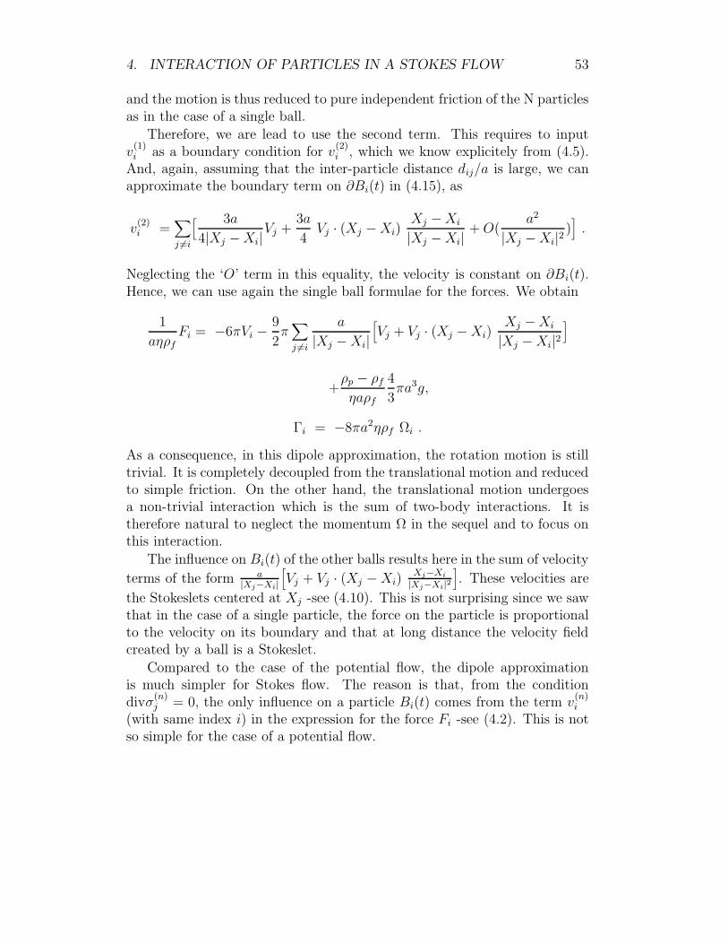
and the motion is thus reduced to pure independent friction of the N particlesas in the case of a single ball.

Therefore, we are lead to use the second term. This requires to inputv

(1)i as a boundary condition for v

(2)i , which we know explicitely from (4.5).

And, again, assuming that the inter-particle distance dij/a is large, we canapproximate the boundary term on ∂Bi(t) in (4.15), as

v(2)i =

∑

j 6=i

[ 3a

4|Xj − Xi|Vj +

3a

4Vj · (Xj − Xi)

Xj − Xi

|Xj − Xi|+ O(

a2

|Xj − Xi|2)]

.

Neglecting the ‘O’ term in this equality, the velocity is constant on ∂Bi(t).Hence, we can use again the single ball formulae for the forces. We obtain

1

aηρf

Fi = −6πVi −9

2π∑

j 6=i

a

|Xj − Xi|

[

Vj + Vj · (Xj − Xi)Xj − Xi

|Xj − Xi|2

]

+ρp − ρf

ηaρf

4

3πa3g,

Γi = −8πa2ηρf Ωi .

As a consequence, in this dipole approximation, the rotation motion is stilltrivial. It is completely decoupled from the translational motion and reducedto simple friction. On the other hand, the translational motion undergoesa non-trivial interaction which is the sum of two-body interactions. It istherefore natural to neglect the momentum Ω in the sequel and to focus onthis interaction.

The influence on Bi(t) of the other balls results here in the sum of velocity

terms of the form a|Xj−Xi|

[

Vj + Vj · (Xj − Xi)Xj−Xi

|Xj−Xi|2

]

. These velocities are

the Stokeslets centered at Xj -see (4.10). This is not surprising since we sawthat in the case of a single particle, the force on the particle is proportionalto the velocity on its boundary and that at long distance the velocity fieldcreated by a ball is a Stokeslet.

Compared to the case of the potential flow, the dipole approximationis much simpler for Stokes flow. The reason is that, from the conditiondivσ

(n)j = 0, the only influence on a particle Bi(t) comes from the term v

(n)i

(with same index i) in the expression for the force Fi -see (4.2). This is notso simple for the case of a potential flow.


5 Kinetic and macroscopic eq. for particles

in a Stokes flow

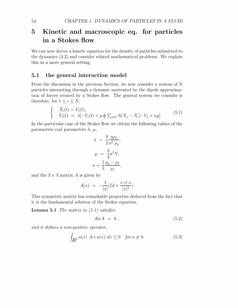
We can now derive a kinetic equation for the density of particles submitted tothe dynamics (4.2) and consider related mathematical problems. We explainthis in a more general setting.

5.1 the general interaction model

From the discussion in the previous Section, we now consider a system of Nparticles interacting through a dynamic motivated by the dipole approxima-tion of forces created by a Stokes flow. The general system we consider istherefore, for 1 ≤ i ≤ N,

Xi(t) = Vi(t),

Vi(t) = λ[−Vi(t) + µ 1N

∑

j 6=i A(Xj − Xi) · Vj + κg].(5.1)

In the particular case of the Stokes flow we obtain the following values of theparameters real parameters λ, µ,

λ =9

2

ηρf

a2 ρp,

µ =3

4a2N,

κ =1

λ

ρp − ρf

ρf,

and the 3 × 3 matrix A is given by

A(x) = −1

|x|[Id +

x ⊗ x

|x|2].

This symmetric matrix has remarkable properties deduced from the fact thatit is the fundamental solution of the Stokes equation.

Lemma 5.1 The matrix in (5.1) satisfies

divA = 0 , (5.2)

and it defines a non-positive operator,∫

IR3 u(x) A ∗ u(x) dx ≤ 0 for u 6= 0. (5.3)

5. KINETIC AND MACROSCOPIC EQ. FOR A STOKES FLOW 55

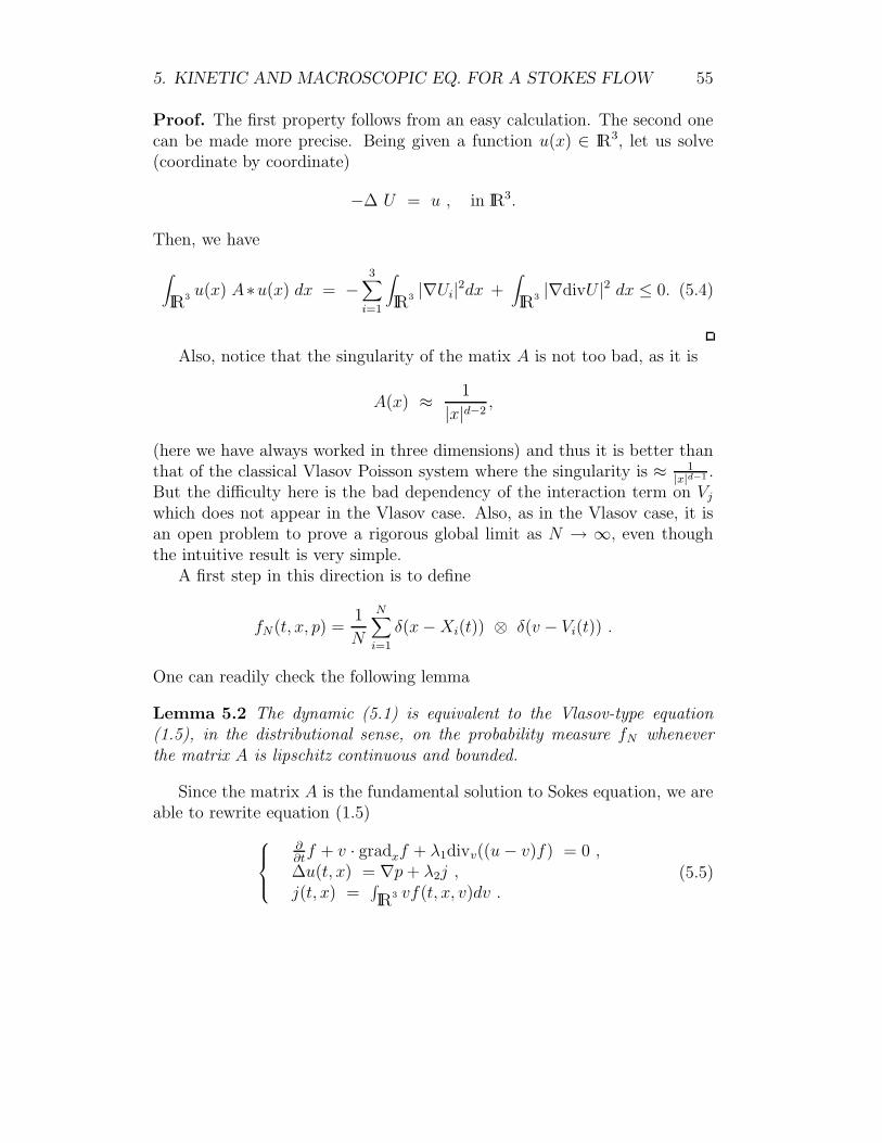
Proof. The first property follows from an easy calculation. The second onecan be made more precise. Being given a function u(x) ∈ IR3, let us solve(coordinate by coordinate)

−∆ U = u , in IR3.

Then, we have

∫

IR3 u(x) A∗u(x) dx = −3∑

i=1

∫

IR3 |∇Ui|2dx +

∫

IR3 |∇divU |2 dx ≤ 0. (5.4)

Also, notice that the singularity of the matix A is not too bad, as it is

A(x) ≈1

|x|d−2,

(here we have always worked in three dimensions) and thus it is better thanthat of the classical Vlasov Poisson system where the singularity is ≈ 1

|x|d−1 .But the difficulty here is the bad dependency of the interaction term on Vj

which does not appear in the Vlasov case. Also, as in the Vlasov case, it isan open problem to prove a rigorous global limit as N → ∞, even thoughthe intuitive result is very simple.

A first step in this direction is to define

fN(t, x, p) =1

N

N∑

i=1

δ(x − Xi(t)) ⊗ δ(v − Vi(t)) .

One can readily check the following lemma

Lemma 5.2 The dynamic (5.1) is equivalent to the Vlasov-type equation(1.5), in the distributional sense, on the probability measure fN wheneverthe matrix A is lipschitz continuous and bounded.

Since the matrix A is the fundamental solution to Sokes equation, we areable to rewrite equation (1.5)

∂∂t

f + v · gradxf + λ1divv((u − v)f) = 0 ,∆u(t, x) = ∇p + λ2j ,j(t, x) =

∫

IR3 vf(t, x, v)dv .(5.5)


This system looks very much like a model used by K. Hamdache (see [18])and other authors which consists in replacing the second equation in theprevious system by

∂tu(t, x) − η∆u = ∇p + λ2(ρu − j) ,ρ(t, x) =

∫

IR3 f(t, x, v)dv .(5.6)

Except for the evolution term ∂tu, the main difference with our equation isthe change of sign for λ2j and the non-linear term λ2ρu which is supposed torepresent the full interaction between particles. Although it is more realistic,this model is also more complicated and in the following we will only deal withthe more simple system (5.5) and usually under the form given by equation(1.5).

5.2 energy and long time behavior for the kinetic equa-

tion

From the energy property of the N -particles system - see also the calculationin the Remark 4.1 - we can hope an energy inequality for the kinetic system(1.5). We define the kinetic energy

EK(t) =1

2

∫

IR6 |v|2f(t, x, v) dv dx ,

then, we have indeed,

ddtEK(t) = λ(−2EK(t) + 2µ

∫

IR3 j A ∗ j dx ,

≤ −2λEK(t) .

This last inequality is a simple consequence of the property (5.4). As aconsequence, we deduce the dissipation rate of kinetic energy

EK(t) ≤ EK(0)e−2λt.

This property is fundamental in the theory developed in P.E. Jabin to provethe following result.

Theorem 5.3 [21] With the matrix A given by (5.1) and g = 0, assume thatthe initial density f(t = 0) has finite energy and

f(t = 0) ∈ L1 ∩ L∞(IR6).

5. KINETIC AND MACROSCOPIC EQ. FOR A STOKES FLOW 57

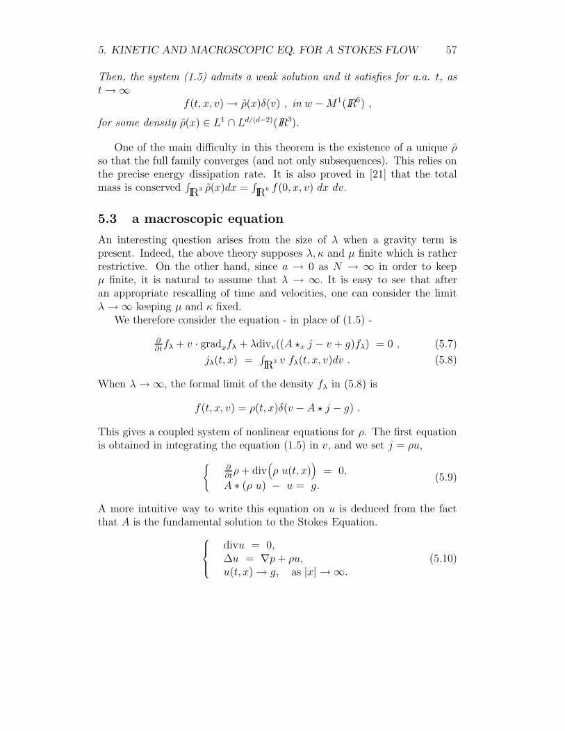
Then, the system (1.5) admits a weak solution and it satisfies for a.a. t, ast → ∞

f(t, x, v) → ρ(x)δ(v) , in w − M 1(IR6) ,

for some density ρ(x) ∈ L1 ∩ Ld/(d−2)(IR3).

One of the main difficulty in this theorem is the existence of a unique ρso that the full family converges (and not only subsequences). This relies onthe precise energy dissipation rate. It is also proved in [21] that the totalmass is conserved

∫

IR3 ρ(x)dx =∫

IR6 f(0, x, v) dx dv.

5.3 a macroscopic equation

An interesting question arises from the size of λ when a gravity term ispresent. Indeed, the above theory supposes λ, κ and µ finite which is ratherrestrictive. On the other hand, since a → 0 as N → ∞ in order to keepµ finite, it is natural to assume that λ → ∞. It is easy to see that afteran appropriate rescalling of time and velocities, one can consider the limitλ → ∞ keeping µ and κ fixed.

We therefore consider the equation - in place of (1.5) -

∂∂t

fλ + v · gradxfλ + λdivv((A ?x j − v + g)fλ) = 0 , (5.7)

jλ(t, x) =∫

IR3 v fλ(t, x, v)dv . (5.8)

When λ → ∞, the formal limit of the density fλ in (5.8) is

f(t, x, v) = ρ(t, x)δ(v − A ? j − g) .

This gives a coupled system of nonlinear equations for ρ. The first equationis obtained in integrating the equation (1.5) in v, and we set j = ρu,

∂∂t

ρ + div(

ρ u(t, x))

= 0,

A ∗ (ρ u) − u = g.(5.9)

A more intuitive way to write this equation on u is deduced from the factthat A is the fundamental solution to the Stokes Equation.

divu = 0,∆u = ∇p + ρu,u(t, x) → g, as |x| → ∞.

(5.10)


From the free divergence condition, we deduce that the transport equationfor ρ shares the basic Lp norm conservation property with the vorticity for-mulation of two dimensional Euler Equations for incompressible flows (see forinstance J.Y. Chemin [11], C. Machioro and M. Pulvirenti [24]). A rigorousderivation of this limit λ → ∞ is given in P.E. Jabin [22].

This kind of ‘macroscopic’ limit of a kinetic equation, without the helpof a collision term is very exceptional compared to the classical relaxationtoward a thermal equilibrium (see [9], [10]). There are other known cases of asimilar phenomena. For instance, let us quote the gyrokinetic limit in plasmaphysics (see E. Frenot and E. Sonnendrucker [13]), the quasi-neutral limit ofVlasov-Poisson Equation (see Y. Brenier and E. Grenier [4], Y. Brenier [5]).

6 Appendix 1. Numerical simulations in the

case of a potential flow and short range ef-

fect

In this Section, we would like to report on some numerical simulations for amore complete problem of particles moving in a potential flow. This allowsto address the question of short range effects and collisions which was leftopen in the sections 3 and 4. Additional results can be found in [6].

To the situation presented in Sections 2 and 3, we add the gravity forcesand the friction term derived in Section 4. This allows more realistic compu-tations. Also, we found it more convenient to work in the physical variables(velocity, not impulsion) and thus to consider the dynamic equation (3.10).This gives the equations of motion

d

dtXi(t) = Vi(t), (6.1)

d

dtVi(t) = γi(t), (6.2)

where the acceleration is given by four different terms

γi(t) = (γ0 + γ1 + γη + γg)(Xi(t)), with (6.3)

γ0(x) = a3τ∑

1≤j≤N

Vj(t)t∇xB(x − Xj(t))Vj(t), (6.4)

γ1(x) = a3τ∑

1≤j≤N

B(x − Xj(t))γ0(Xj(t)), (6.5)

6. APPENDIX 1. SIMULATIONS FOR A POTENTIAL FLOW 59

γη(x) = −12πηa(Vi(t) − vf (x)

43πa3(ρp +

ρf

2)

, (6.6)

γg(x) =ρp − ρf

ρp + ρf/2g. (6.7)

The first two terms represent the added mass force (3.10) with a second orderapproximation in the kinetic parameter λ in (2.1), which has the property topreserv the right energy structure (cf. [19], [6]). We recall the definition ofB in (3.4). The term γη represents the friction due to viscosity and the lastterm is the buoyant force (poussee d’Archimede). The fluid velocity is takenaccording to the potential gradient, deduced from Section 2,

vf(x) = 2πa3∑

1≤j≤N

B(x − Xj(t)) [ Vj(t)

−2πa3∑

1≤k≤N

B(Xj(t) − Xk(t))Vk(t) ]. (6.8)

But a fundamental effect in this motion is that particles have a tendencyto collide much more than expected from the classical rate of collision na2.This is due to the fact that particles moving with parallel velocities (this isfrequent due to gravity) have a tendency to attract each other. Thereforeit is fundamental to introduce collision rules. These have been taken as theusual hard-sphere collisions; postcollisional velocities are given by

V ′i = Vi − [(Vi − Vj) · n] n

V ′j = Vj + [(Vi − Vj) · n] n,

where n denotes the normal n =xi−xj

|xi−xj |. This is possible because we work

directly in physical variables. In the impulsion variables this is also possible(see [32], [27])

We performed numerical tests In figures 1 and 2 we presente a three di-mensional evolution of 125 bubbles, initially semiregularly distributed arounda 5x5x5 grid, with velocity zero.

The physical data are: diameter = 10−3m, concentration = 12.7% (thiscorresponds to a box which side is 8mm long), gravity = −9.81ez, viscosity= 10−3Pa.s, ρf = 1000kg/m3, ρp = 0.

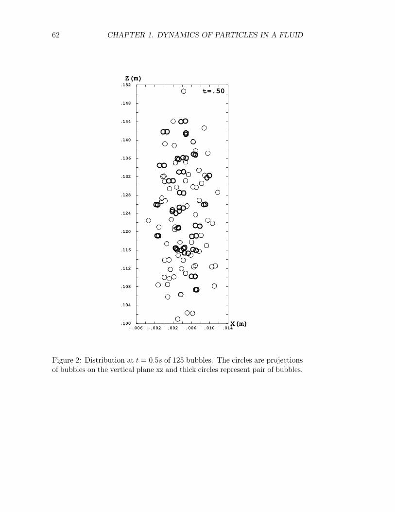
First, we observe the formation of horizontal continuous layers, normalto gravity (this is due to attraction of bubbles lifting in the same horizon-tal plane) next, a vertical repulsion between layers destabilize their shape.


Finally we obtain, when bubbles reach their limit velocity (due to friction)a cloud of dispersed bubbles or pairs of bubbles (rather normal to gravity)elongated in the gravity direction. Especially, including the real collisions,we do not observe anymore the strong horizontal layering. This effect hasbeen obtained with a modification of the short range forces to make themrepulsive (see [19], [29], [30]). The main macroscopic effect rather comes fromparticles stiking together as can be seen in figures 1 and 2 (thick cicles arethose touching each other in the three dimensional space).

Acknowledgment We would like to thank J.F. Bourgat and INRIA (projectM3N) for providing the numerical results in the Appendix, as well as B.Lucquin for a constant help in developing the numerical code.

6. APPENDIX 1. SIMULATIONS FOR A POTENTIAL FLOW 61

-.002 .000 .002 .004 .006 .008 .010-.001

.001

.003

.005

.007

.009

.011

X(m)

Z(m)

t=.00

-.002 .000 .002 .004 .006 .008 .010.001

.003

.005

.007

.009

.011

.013

X(m)

Z(m)

t=.02

-.002 .000 .002 .004 .006 .008 .010.004

.006

.008

.010

.012

.014

.016

.018

.020

.022

.024

.026

.028

X(m)

Z(m)

t=.05

-.002 .000 .002 .004 .006 .008 .010

.012

.014

.016

.018

.020

.022

.024

.026

.028

.030

.032

.034

.036

X(m)

Z(m)

t=.10

Figure 1: Snapshots of the evolution of 125 bubbles initially semiregularlydistributed in a box, with velocity zero, at t=0., 0.02, 0.05, 0.1s. The circlesare projections of bubbles on the vertical plane xz and thick cercles representpairs or group of bubbles.


-.006 -.002 .002 .006 .010 .014.100

.104

.108

.112

.116

.120

.124

.128

.132

.136

.140

.144

.148

.152

X(m)

Z(m)

t=.50

Figure 2: Distribution at t = 0.5s of 125 bubbles. The circles are projectionsof bubbles on the vertical plane xz and thick circles represent pair of bubbles.

7. APPENDIX 2. SIMULATIONS FOR A STOKES FLOW 63

7 Appendix 2 : numerical simulations for a

Stokes flow

7.1 Introduction

We present here some numerical simulations for the simplified model of par-ticles in a Stokes flow detailed in section 5.1 under the form of a kineticequation for the dynamics of the particles. The purpose of this appendix ismainly to investigate numerically the long time behaviour of this equationin the case where there is gravity.

In the case without gravity, the result is known (see section 5.2 ) andthe solution concentrates towards zero velocities. It should be noticed thatequation 1.5 is not invariant under galilean transformations. This simplycomes from our assumption that the fluid is at rest at infinity. Because ofthis lack of galilean invariance in the equation, we cannot reduce the casewith gravity to the case without gravity.

However even with this remark, one does not expect a completely dif-ferent behaviour for the cases with or without gravity. Hence a reasonableconjecture for the case with gravity could have been the following

Conjecture 1 The solution f to equation 1.5 converges weakly to ρδ(v−v0)for some ρ(x) and v0(x) depending on the parameters of the equation andpossibly the initial data.

A weaker conjecture could also be as follows.

We define the functional

F (t) =∫

IR6 |v − vm|2f(t, x, v)dxdv , (7.1)

where vm is the average velocity

vm(t) =(∫

IR6 vf(t, x, v)dxdv)

/(∫

IR6 fdxdv)

. (7.2)

Conjecture 2 The solution to equation 1.5 concentrates in velocity in longtime. More precisely, vm tends to some v0 and the functionnal F just definedin ( 7.1 ) converges to zero as the time goes to infinity.

As surprising (or unsurprising) as it may seem, these two conjecturescannot be numerically verified at all. Based on numerical evidences, theasymptotic behaviour is thus completely different when we add a gravity.


7.2 Presentation of the computation

We solve numerically the system

d

dtXi(t) = Vi(t), (7.3)

d

dtVi(t) = −λVi(t) +

1

N

N∑

j=1

Aη(Xj − Xi) · Vj + g. (7.4)

(7.5)

This corresponds to the system 5.1 normalized with µ = κ = 1λ

exceptthat in the interaction term of 7.4 the sum is done for all indices j includingi. The matrix Aη is a regularisation of the matrix A defined in section 5.1,more precisely

Aη(x) = −1

|x| + η

(

Id +x ⊗ x

(|x| + η)2

)

. (7.6)

In the simulations presented further, λ and η are chosen equal to 0.1, g isthe vector (0, 0, 1) and we take 200 particles.

Solving numerically the previous system presents no significant problemonce you have chosen a time step small enough for stability. Moreover by op-position to the case of a potential flow, short range effects are not importanthere. In fact, although the interaction does not completely prevent them,collisions are very rare and usually the particles remain far enough from eachother.

We have considered three kinds of initial conditions. The first one cor-responds to random position in the cube [0, 1]3 and random velocities in[−30, 30]3. The second one consists in taking Xi(0) = (i − 1, 0, 0) andVi(0) = (0, 0, 1), and the last one Xi(0) = (i−1, 0, 0) and Vi(0) = (0, 0, i−1).

7.3 Conclusions

The figures below clearly show that the velocity fluctuation F (t) does notvanish. On other tests which we do not present here, we never observed aconcentration of velocities.

Another computation, not shown here, concerns the minimal distancebetween particles. We indeed checked that collisions are extremely rare :particles never come close to each other.


Acknowledgements. We did these simulations during a stay at the ErwinSchrodinger Institute in Vienna and we would like to thank the members ofthe Institute and especially P. Pietra for her help and advices.


0 50 100 150 200 2500

20

40

60

80

100

120

140

160

180

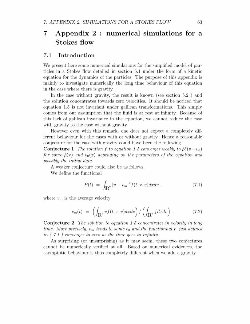
Figure 3: concentration in velocity F (t) = 1N

∑Ni=1 |Vi(t) − Vm(t)|2, with

Vm = 1N

∑Ni=1 Vi(t), in the case of random initial positions and velocities.

This seems to indicate that F (t) converges towards zero but it is false as thenext picture shows it.


0 50 100 150 200 2500

0.01

0.02

0.03

0.04

0.05

0.06

0.07

0.08

0.09

0.1

Figure 4: same as figure 1 but rescaled along the vertical axis. The functionalF (t) stops decreasing after a while.


0 200 400 600 800 1000 1200 1400 1600 1800 20000

0.1

0.2

0.3

0.4

0.5

0.6

0.7

0.8

Figure 5: concentration in velocity F (t) = 1N

∑Ni=1 |Vi(t) − Vm(t)|2, with

Vm = 1N

∑Ni=1 Vi(t), with Xi(0) = (i − 1, 0, 0) and Vi(0) = (0, 0, 1). Again

F (t) does not converges towards zero. The stabilisation time and level arequite different from the previous picture, and therefore it is not due to anumerical artefact.

0 500 1000 1500 2000 2500 3000 3500 4000 4500 5000−0.01

−0.005

0

0.005

0.01

0.015

0.02

0.025

Figure 6: first coordinate of the average velocity Vm, with Xi(0) = (i−1, 0, 0)and Vi(0) = (0, 0, 1). The fluctuation never vanishes.


−50

510

1520

−1

−0.5

0

0.5

1600

700

800

900

1000

1100

1200

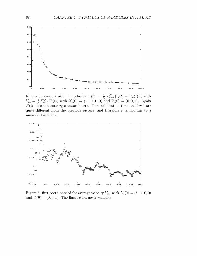
Figure 7: this picture shows the position of all the particles at time 200, withinitial repartition Xi(0) = (i − 1, 0, 0) and Vi(0) = (0, 0, i − 1).


−800−600

−400−200

0200

400600

−1

−0.5

0

0.5

15

5.2

5.4

5.6

5.8

6

6.2

6.4

6.6

x 104

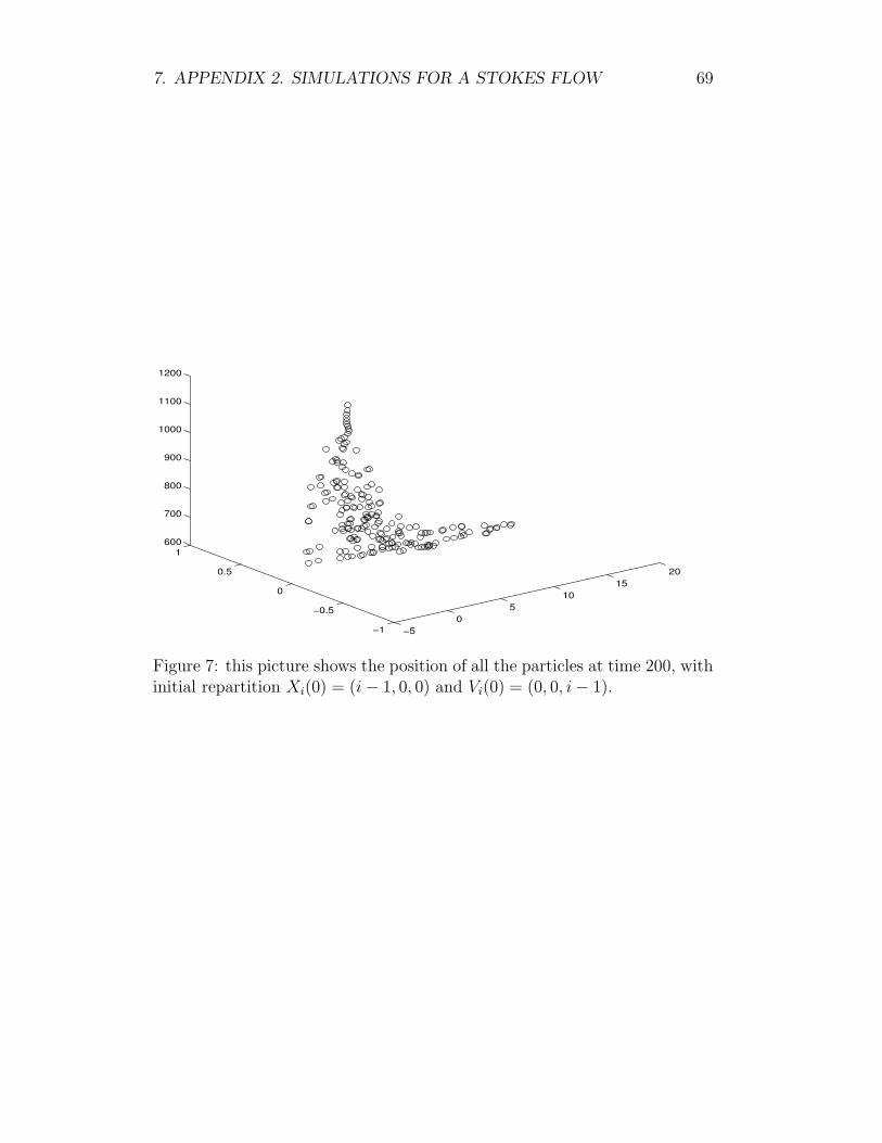
Figure 8: this picture shows the position of all the particles at time 10000,with initial repartition Xi(0) = (i − 1, 0, 0) and Vi(0) = (0, 0, i − 1).

REFERENCES 71

References

[1] V.I. Arnold, Mathematical Methods of Classical Mechanics,Grad. Texts. Math. 60, Springer, (1978).

[2] G.K. Batchelor, An Introdution to Fluid Dynamics, CambridgeUniversity Press, (1967).

[3] D. Benedetto, E. Caglioti and M. Pulvirenti, A kineticequation for granular media, M2AN, Vol. 31(5) (1997), 615–642.

[4] Y. Brenier, E. Grenier, Limite singuliere du systeme deVlasov-Poisson dans le regime de quasineutralite: le cas indepen-dant du temps, C. R. Acad. Sc. Paris, t. 318, Serie I (1994)121–124.

[5] Y. Brenier, Convergence of the Vlasov-Poisson system to theincompressible Euler equations, to appear in C.P.D.E.

[6] J.F. Bourgat, B. Lucquin-Desreux and B. Perthame,Motion of dispersed bubbles in a potential flow. 21st Int. Symp.on Rarefied Gas Dynamics. Marseilles, July 1998.

[7] H.F. Bulthuis, A. Prosperetti and A.S. Sangani, Particlestress in disperse two-phase potential flow, J. Fluid Mech., vol.294 (1995) 1–16.

[8] G.K. Batchelor and C.S. Wen, Sedimentation in a dilutepolydispersed system of interacting spheres, J. Fluid Mech. 124,(1982) 495–528.

[9] C. Cercignani, The Boltzmann equation and its application, Ap-plied Math. Sciences 67, Springer–Verlag , Berlin (1988).

[10] C. Cercignani, R. Illner and M. Pulvirenti, The math-ematical theory of dilute gases, Applied Math. Sciences 106,Springer–Verlag , Berlin (1994).

[11] J.Y. Chemin, Fluides parfaits incompressibles, Asterisque 230,S.M.F. (1995).


[12] F. Feuillebois, Sedimentation in a dispersion with vertical in-homogeneities, J. Fluid Mech. 139, (1984) 145–172.

[13] E. Frenod and E. Sonnendrucker, Long time behaviour ofthe two-dimensional Vlasov equation with a strong external mag-netic field, INRIA report 3428, (1998).

[14] R.T. Glassey, The Cauchy problem in kinetic theory, SIAM pub-lications, Philadelphia (1996).

[15] R. Glowinski, T.W. Pan and J. Periaux, A fictitious do-main method for external incompressible viscous flow modeledby Navier-Stokes equations, Comput. Meth. Mech. Engnr. 112,(1994), 133–148.

[16] E.J. Hinch, An averaged-equation approach to particle interac-tions in a fluid suspension, J. Fluid Mech. 83, (1977) 695–720.

[17] J. Happel and H. Brenner, Low Reynolds Number Hydrody-namics, Prentice-Hall, (1965).

[18] K. Hamdache, Global existence and large time behaviour of so-lutions for the Vlasov-Stokes equations, Japan J. Ind. and Appl.Math. To appear.

[19] H. Herrero, B. Lucquin-Desreux and B. Perthame, Onthe motion of dispersed bubbles in a potential flow -a kinetic de-scription of the added mass effect, Publ. Lab. An. Num. Paris VI.

[20] R. Herczynski and I. Pienkowska, Towards a statistical the-ory of suspension, Ann. Rev. Fluid Mech. 12, (1980) 237–269.

[21] P.E. Jabin, Large time concentrations for solutions to kineticequations with energy dissipation, Com. in P.D.E. To appear.

[22] P.E. Jabin, Doctoral Dissertation, Univ. Paris 6. In preparation.

[23] P.L. Lions, B. Perthame and E. Tadmor, Kinetic formu-lation of isentropic entropy solutions to isentropic gas dynamicssystem in Eulerian and Lagrangian variables, Comm. Math. Phys.163 (1994) 415–431.

REFERENCES 73

[24] C. Marchioro and M. Pulvirenti, Vortex method in two-dimensional fluid dynamics, Lecture Notes in Physics, 203,Springer (1984).

[25] B. Maury, R. Glowinski, Fluid particle flow: a symmetricformulation, C. R. Acad. Sci. Paris, t. 324, Serie I, p. 1079-1084,1997.

[26] G. Russo and P. Smereka, Kinetic theory for bubbly flow I:collisionless case, SIAM J. Appl. Math., Vol. 56, n2 (1996), 327–357.

[27] G. Russo and P. Smereka, Kinetic theory for bubbly flow II:fluid dynamic limit, SIAM J. Appl. Math., Vol. 56, n2 (1996),358–371.

[28] A. S. Sangani and A.K. Didwania, Dispersed-phase stresstensor in flows of bubbly liquids at large Reynolds numbers, J.Fluid Mech., vol. 248 (1993), 27–54.

[29] A. S. Sangani and A.K. Didwania, Dynamic simulations offlows of bubbly liquids at large Reynolds numbers, J. Fluid Mech.,vol. 250 (1993), 307–337.

[30] P. Smereka, On the motion of bubbles in a periodic box, J. FluidMech. 254 (1993) 79–112.

[31] H. Spohn, Large scale dynamics of interacting particles, Springer-Verlag, Berlin, (1991).

[32] Y. Yurkovetsky, J.F. Brady, Statistical mechanics of bubblyliquids, Phys. Fluids 8 (4), (1996) 881-895.

notes on mathematical problems on the dynamics of ...jabin/particlesinfluid3.pdf36 chapter 1....

Documents