Notes on Landau dampingby Youjun Hu

Institute of Plasmas, Chinese Academy of SciencesEmail: yjhu@ipp.cas.cn

In Sec. 1 of this note, resonant wave particle interactions are demonstrated by a simple test-particle simulation. Section 2 reproduces Stix's derivation of Landau damping from the view oftest particles[4]. In Sec. 3, linearized Vlasov-Poison equations are solved numerically to demon-strate the �phase mix� in velocity space and the resulting Landau damping.

1 Test-particle simulation of Landau damping

Consider a longitudinal wave given by

E= zE cos(kz¡!t): (1)

The equations of motion of a test particle in the wave �eld are given by

mdv

dt= qE cos(kz¡!t); (2)

anddzdt

= v; (3)

where v�v � z is the z component of the velocity of the particle.Normalize z by the wavelength �, t by the wave period T , v by the phase velocity vp, i.e.,

z=z�; t=

tT; v=

vvp; (4)

where � = 2� /k, T = 2� /!, vp = ! /k. Using the normalized quantities, Eqs. (2) and (3) arewritten, respectively, as

d vd t

=2�kqEm!2

cos[2�(z¡ t)]; (5)

andd zd t

=v: (6)

The initial distribution function of particles f0(z; v) is taken to be uniform in space andMaxwellian in velocity,

f0(z; v)= fm(v)=1

vt 2�p exp

�¡ v2

2vt2

�; (7)

which satis�es the normalization conditionR¡11

f0(v)dv = 1 (Note that here vt = T /mp

, which

is di�erent from the usual de�nition vt = 2T /mp

used Sec. 3.4 of this note). In my particlesimulation code (/home/yj/project_new/pic_code), 4 � 105 particles are initially loadedrandom in z and Maxwellian in v. Then the motion equations of every particle are followednumerically to obtain the location and velocity at later time. In the numerical code, when a par-ticle leaves from the region 0 6 x 6 1, it is shifted by one wavelength to return to this region.This shift does not in�uence the force on the particle and it simulates the situation of in�nitelength in z direction, where when a particle leave the region 06 x 6 1 from the right boundary,a particle of the same velocity will enter the region from the left boundary, and vice versa.

1

The velocity distribution at later time is obtained by counting the number of particles ineach velocity interval. Figure 1a compares the velocity distribution function at t= 0 and t = 10,which shows that the distribution is �atted in the resonant region v/vp= 1, which suggests thatthe total kinetic energy of particles may be increased. Figure 2 plots the temporal evolution ofthe total kinetic energy of the particles, which con�rms that the kinetic energy is increased bythe wave. The conservation of energy tell us that the increased kinetic energy of particles mustbe drawn from the wave, i.e., the wave encounters damping.

0

0.1

0.2

0.3

0.4

0.5

0.6

-3 -2 -1 0 1 2 3

(a)

velo

city

dis

trib

utio

n fu

nctio

n

v/vp

t=0t/T=10

0

0.1

0.2

0.3

0.4

0.5

0.6

-3 -2 -1 0 1 2 3

velo

city

dis

trib

utio

n fu

nctio

n

v/vp

t=0t/T=1t/T=5

t/T=10t/T=20

Figure 1. Comparison of the velocity distribution function (spatially averaged) at various time, whichshows that the distribution is distorted in the resonant region (v / vp � 1). Other parameters: vt / vp = 1,2�kqE/m!2=1.

1

1.02

1.04

1.06

1.08

1.1

1.12

1.14

0 5 10 15 20

Ek

t/T

Figure 2. Temporal evolution of the total kinetic energy of the particles, where Ek =P

i=1i=N 1

2mvi

2 /�N

1

2mvt

2�. Other parameters: vt/vp=1, 2�kqE/m!2=1.

Although the above simulation is performed by holding the wave amplitude constant, it takesinto account all the nonlinear physics of the particle motion in the wave �eld. Therefore this is anonlinear simulation.

1.1 Linear Landau dampingIn the early phase of the simulation

t� 2�p

/!b; (8)

where !b is the bounce angular frequency of particles in the trough of the wave, the trappedparticles e�ects can be neglected. This phase can be considered as the linear phase where thelinear Landau damping theory (discussed later in this note) is valid. The bounce angular fre-quency of particles in the trough of the wave is given by[1]

!b=kqEm

r: (9)

2 Section 1

Using this, the condition (8) is written as

tT� m!2

2�kqE

r: (10)

This condition reduces to t /T � 1 for the case plotted in Fig. 2, where we see that the totalkinetic energy of the particles increases monotonously with time during this period. From thedata in Fig. 2, the temporal change rate of the total kinetic energy can be computed, whichgives d Ek/dt = 0.08. Next, I compare this result with those given by the analytic formula (39)(given later in this note), which is written

dEkdt

=¡ �!jk jk

(qE)2

2m

�df(v0)dv0

�v0=!/k

:

Using Eq. (7) and vt/vp=1, the above expression is written

dEkdt

=�(qE)2

2m!1

2�p exp

�¡12

�Multiplying by T and then dividing by mvt

2/2, the above expression is written

dEkd t

=4�2(kqE)2

m2!41

2 2�p exp

�¡12

�In the simulation 2�kqE/m!2=1. Using this, expression (10) is written as

dEkd t

=1

2 2�p exp

�¡12

�= 0.12

The result given by the analytic formula is slightly di�erent from that of the simulation (0.12 vs0.08). Considering the various approximations used in deriving the analytic formula, the tworesults can be considered to be in agreement with each other.

1.2 Nonlinear Landau damping

In the phase after the linear phase, Fig. 2 indicates that the total kinetic energy of the particlesoscillates with time, with the saturation level larger than the initial kinetic energy of the parti-cles, i.e., there is nonzero net energy drawn from the wave by the particles. This is the nonlinearLandau damping, which clearly demonstrates that net energy exchange between waves and par-ticles can be nonzero on the long time scale without including any collisional e�ect.

1.3 Inverse Landau damping

Choose a drift-Maxwellian distribution

f0(z; v)= fm(v)=1

vt 2�p exp

�¡(v¡ vb)

2

2vt2

�; (11)

with vb/ vp = 2. Then the derivative of the distribution function with respect to the velocity inthe resonant region is positive. This is the case where an inverse Landau damping is expected toappear. Figure 3 compares the velocity distribution function at t = 0 and t = 10, which showsthat the distribution is �atted in the resonant region v/vp= 1. Figure 4 plots the temporal evo-lution of the total kinetic energy of the particles, which confirms that the kinetic energy isreduced by the wave.

Test-particle simulation of Landau damping 3

0

0.05

0.1

0.15

0.2

0.25

0.3

0.35

0.4

-2 -1 0 1 2 3 4 5 6

(a)

velo

city

dis

trib

utio

n fu

nctio

n

v/vp

t=0t/T=10

Figure 3. Comparison of the velocity distribution function (spatially averaged) at various time, whichshows that the distribution is distorted in the resonant region (v /vp � 1). Other parameters: vt/vp = 1,2�kqE/m!2=1.

0.975

0.98

0.985

0.99

0.995

1

1.005

0 5 10 15 20

Ek

t/T

Figure 4. Temporal evolution of the total kinetic energy of the particles, where Ek=Pi=1i=N 1

2mvi

2/Ek0,Ek0 is the initial total kinetic energy. Other parameters: vt/vp=1, 2�kqE/m!2=1.

1.4 Density �uctuation induced by the waveFigure (5) compares the spatial distribution at t= 0 and t= 10T , which shows that the distribu-tion become nonuniform at t= 10T .

0.9

0.95

1

1.05

1.1

1.15

0 0.1 0.2 0.3 0.4 0.5 0.6 0.7 0.8 0.9 1

spat

ial d

istr

ibut

ion

func

tion

x/λ

t=0t/T=10

Figure 5. Comparison of the spatial distribution function at t= 0 and t= 10, which shows that the dis-tribution seems to become nonuniform at t= 10. Other parameters: vt= vp, 2�kqE/m!2=1.

4 Section 1

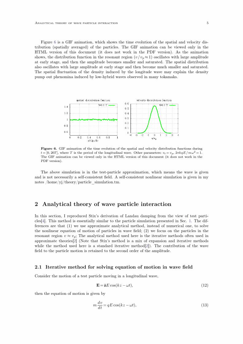
Figure 6 is a GIF animation, which shows the time evolution of the spatial and velocity dis-tribution (spatially averaged) of the particles. The GIF animation can be viewed only in theHTML version of this document (it does not work in the PDF version). As the animationshows, the distribution function in the resonant region (v/vp� 1) oscillates with large amplitudeat early stage, and then the amplitude becomes smaller and saturated. The spatial distributionalso oscillates with large amplitude at early stage and then become much smaller and saturated.The spatial �uctuation of the density induced by the longitude wave may explain the densitypump out phenomina induced by low-hybrid waves observed in many tokamaks.

Figure 6. GIF animation of the time evolution of the spatial and velocity distribution functions duringt= [0; 20T ], where T is the period of the longitudinal wave. Other parameters: vt= vp, 2�kqE /m!2= 1.The GIF animation can be viewed only in the HTML version of this document (it does not work in thePDF version).

The above simulation is in the test-particle approximation, which means the wave is givenand is not necessarily a self-consistent �eld. A self-consistent nonlinear simulation is given in mynotes /home/yj/theory/particle_simulation.tm.

2 Analytical theory of wave particle interaction

In this section, I reproduced Stix's derivation of Landau damping from the view of test parti-cles[4]. This method is essentially similar to the particle simulation presented in Sec. 1. The dif-ferences are that (1) we use approximate analytical method, instead of numerical one, to solvethe nonlinear equation of motion of particles in wave �eld; (2) we focus on the particles in theresonant region v � vp; The analytical method used here is the iterative methods often used inapproximate theories[2] (Note that Stix's method is a mix of expansion and iterative methodswhile the method used here is a standard iterative method[2]). The contribution of the wave�eld to the particle motion is retained to the second order of the amplitude.

2.1 Iterative method for solving equation of motion in wave �eld

Consider the motion of a test particle moving in a longitudinal wave,

E= zE cos(kz¡!t); (12)

then the equation of motion is given by

mdvdt

= qE cos(kz ¡!t); (13)

Analytical theory of wave particle interaction 5

anddzdt

= v; (14)

with initial condition v(0) = v0 and z(0) = z0, where v� v � z and v is the velocity of the particle.Equations (13) and (14) are nonlinear system, for which exact solutions are hard to be found.Here, we consider the amplitude of the electrical �eld, E, as a small perturbation, and use theiterative method[2] to solve Eqs. (13) and (14) approximately. The initial guess of the solutionis obtained by setting E=0, which gives

v(0)= v0; (15)

and

z(0)= z0+ v0t: (16)

Substituting this solution back into the right-hand side of Eq. (13), we obtain

mdv(1)

dt= qE cos(kz0+ kv0t¡!t); (17)

which can be integrated over time to give

v(1)= v0+qEm

sin(kz0+�t)¡ sin(kz0)�

; (18)

where �= kv0¡ ! and use has been made of the initial condition v(1)(0) = v0. Substituting thissolution for the velocity, Eq. (14) is written

dz(1)

dt= v0+

qEm

sin(kz0+�t)¡ sin(kz0)�

; (19)

which can be integrated over time, giving

z(1) = z0+ v0t+qEm

Z0

t sin(kz0+�t)¡ sin(kz0)�

dt;

= z0+ v0t+qEm

Z0

t sin(kz0+�t)¡ sin(kz0)�2

d(kz0+�t);

= z0+ v0t+qE

m

�¡cos(kz0+�t)+ cos(kz0)

�2¡ sin(kz0)

�t

�; (20)

where use has been made of the initial condition z(1)(0) = z0. Substituting the solution in Eq.(20) back into the right-hand side of Eq. (13), we obtain

mdv(2)

dt= qE cos(kz(1)¡!t)

= qE cos�kz0+ kv0t+ k

qEm

�¡cos(kz0+�t)+ cos(kz0)

�2¡ t sin(kz0)

�

�¡!t

�= qE cos

�kz0+�t+ k

qEm

�¡cos(kz0+�t)+ cos(kz0)

�2¡ sin(kz0)

�t

��: (21)

Since E is considered to be a small parameter, the term proportional to E can be considered tobe small when compared with kz0 + �t. Therefore, we expand the �rst cosine function in thevicinity of kz0+�t. Thus the above equation is written approximately as

mdv(2)

dt� q E cos(k z0 + �t) ¡ sin(k z0 + �t)k

(qE)2

m

�¡cos(kz0+ �t) + cos(kz0)

�2¡

sin(kz0)�

t

�: (22)

6 Section 2

Next, calculate the time change rate of the kinetic energy of the particle, which is written as

ddt

�12mv2

�= mv

dvdt

� mv(1)dv(2)

dt(23)

Using Eq. (18) for v(1) and Eq. (22) for mdv(2)/dt, Eq. (23) is written

ddt

�12mv2

���v0+

qEm

sin(kz0+�t)¡ sin(kz0)�

���qE cos(kz0 + �t) ¡ sin(kz0 + �t)k

(qE)2

m

�¡cos(kz0+�t) + cos(kz0)

�2¡

sin(kz0)�

t

��� v0qE cos(kz0+�t)

¡ v0sin(kz0+�t)k(qE)2

m

�¡cos(kz0+�t) + cos(kz0)

�2¡ sin(kz0)

�t

�+

(qE)2

msin(kz0+�t)¡ sin(kz0)

�cos(kz0+�t); (24)

where the terms of order E3 have been neglected (if terms of order E3 and higher are included,then the result will correspond to nonlinear Landau damping, is this correct?). Equations (24)agrees with Eq. (8) in Chapter 8 of Stix's book[4] (however Stix's formula misses, by mistakes,the �rst term of the above equation).

2.2 Averaging over initial spatial location and velocity of particles

Assume the distribution function of the particles is given by F (v0; z0) = f(v0)h(z0) and h(z0)= 1,i.e. the distribution is uniform in space.

Consider the averaging over the initial position of particles. De�ne

h:::iz0�k2�

Z0

2�/k

(:::)h(z0)dz0; (25)

which is an operator averaging over the initial position of particles in the interval of one wavelength. Using this operator on both sides of Eq. (24), we obtain�ddt

�12mv2

��z0

= hv0q E cos(k z0 + �t)i ¡�sin(k z0 +

�t)k v0(qE)2

m

�¡cos(kz0+ �t) + cos(kz0)

�2¡ sin(kz0)

�t

��+�

(qE)2

msin(kz0+�t)¡ sin(kz0)

�cos(kz0+�t)

�(26)

= 0 ¡ k2�k v0

(qE)2

m

Z0

2�/k

sin(k z0 + �t)

�¡cos(kz0+ �t) + cos(kz0)

�2¡

sin(kz0)�

t

�d z0 +

k2�

(qE)2

m

Z0

2�/k sin(kz0+ �t)¡ sin(kz0)�

cos(k z0 +

�t)dz0: (27)

Note that the term v0qE cos(kz0 + �t) corresponds to the power of the electric �eld acting onthose particles that move at a constant speed v0. Also note this term is reduced to zero whenaveraged over the initial position z0 no mater whether it is a resonant particle (i.e., �� 0) or not(i.e., �=/ 0). (This important fact is seldom mentioned in textbooks, which is one of the motiva-

Analytical theory of wave particle interaction 7

tions that I wrote this note.) Changing to the new variable x � kz0 + �t, the above equation iswritten as�ddt

�12mv2

��z0

= ¡ k2�kv0

(qE)2

m

Z�t

2�+�t

sin(x)�¡cos(x)+ cos(x¡�t)

�2¡ sin(x¡�t)

�t

�1kdx +

k

2�

(qE)2

m

Z�t

2�+�t sin(x)¡ sin(x¡�t)�

cos(x)1

kdx

= ¡ 12�k v0

(qE)2

m

Z�t

2�+�t

sin(x)�

cos(x¡ �t)�2

¡ sin(x¡ �t)�

t

�d x ¡

12�

(qE)2

m

Z�t

2�+�t sin(x¡�t)�

cos(x)dx

= ¡ 12�kv0

(qE)2

m

�1�2

Z�t

2�+�t

sin(x)cos(x ¡ �t)dx ¡ t�

Z¡�t

2�¡�tsin(x)sin(x ¡

�t) dx

�¡ 12�

(qE)2

m1�

Z�t

2�+�t

sin(x¡�t)cos(x)dx

= ¡ 12�kv0

(qE)2

m

h��2

sin(�t)¡ t��cos(�t)

i+

12�

(qE)2

m1��sin(�t)

=(qE)2

2m

�¡kv0

1�2

sin(�t)+ kv0t�cos(�t) +

1�sin(�t)

�=

(qE)2

2m

�¡(�+!)

1�2

sin(�t)+ (�+!)t�cos(�t) +

1�sin(�t)

�(28)

=(qE)2

2m

h¡ !�2

sin(�t) + t cos(�t)+!t�cos(�t)

i; (29)

which agrees with Eq. (8) in Chapter 8 of Stix's book. Next, we will average Eq. (29) over thedistribution of initial velocity. De�ne the averaging operator in velocity space

h:::iv0=Z¡1

1(:::) f(v0)dv0; (30)

where f(v0) is the one-dimensional distribution function, which satis�es the following normal-izing condition Z

¡1

1f(v0)dv0=1: (31)

Changing to the variables �� kv0¡!, equation (30) is written as

h:::iv0=1jk j

Z¡1

1(:::) f

��+!k

�d�; (32)

De�ne

g(�)� f��+!

k

�: (33)

then equation (32) is written as

h:::iv0=1jk j

Z¡1

1(:::)g(�)d�; (34)

Taking the average over the initial velocity, Eq. (29) is written as��ddt

�12mv2

��z0

�v0

=

�(qE)2

2m

h¡ !�2

sin(�t)+ t cos(�t)+!t�cos(�t)

i�v0

=1jk j

(qE)2

2m

Z¡1

1h¡ !�2

sin(�t)+ t cos(�t)+!t�cos(�t)

ig(�)d� (35)

It can be proved that the integrationR¡11

t cos(�t)g(�)d� andR¡11 t

�cos(�t)g(�)d� in the above

equation approach zero rapidly for large t (refer to Sec. 2.5.3). Thus, in the sense of timeasymptotic, we are left with only the integration of the �rst term, which is written as

¡ 1jk j

(qE)2

2m

Z¡1

1 !�2

sin(�t)g(�)d�: (36)

8 Section 2

2.3 Resonant particles

Since there is a 1/�2 factor in the integrand of the above integral, the important contribution tothe integral must come from the vicinity of � = 0 (i.e. resonant particles). Therefore we expandg(�) as

g(�)= g(0)+ g 0(0)�+ g 00(0)�2

2+ ::: (37)

Since sin(�t) / �2 is odd in �, only terms that are also odd need to be retained in the aboveexpansion. Using these, expression (36) is written as

¡ 1jk j

(qE)2

2m

Z¡1

1 !�2

sin(�t)g(�)d� � ¡ 1jk j

(qE)2

2m

Z¡1

1 !�2

sin(�t)(g 0(0)�)d�

= ¡ 1jk j

(qE)2

2mg 0(0)!

Z¡1

1 1�sin(�t)d�

= ¡ 1jk j

(qE)2

2mg 0(0)!�

= ¡ �!jk jk

(qE)2

2m

�df(v0)dv0

�v0=!/k

: (38)

Using these results, Eq. (35) is written as��ddt

�12mv2

��z0

�v0

�¡ �!jk jk

(qE)2

2m

�df(v0)dv0

�v0=!/k

: (39)

which agrees with Eq. (16) in Chapter 8 of Stix's book[4]. Equation (39) indicates that the timerate of change of the averaged kinetic energy of resonant particles is proportional to the deriva-tive of the initial distribution function at the phase velocity of the wave.

2.4 Wave damping

If the longitudinal wave is an electron plasma wave, then the wave energy consists of two com-ponents, the energy of the electric �eld and the averaged kinetic energy of the particle oscilla-tions,

W =WE+Wp; (40)

where WE is the energy density of the electric �eld averaged in one wavelength, which is givenby

WE=k2�

Z0

2�/k"02[E cos(kx)]2dx=

14"0E

2; (41)

Wp is the averaged kinetic energy of the particle oscillations, which, for electron plasma wave, isequal to the electric �eld energy WE[3]. Using these results, equation (40) is written

W =12"0E

2: (42)

The energy conservation requires that the kinetic energy gained by the resonant particles mustcome from the wave energy, i.e.,

dW

dt=

�!

jk jk(qE)2

2m

�df(v0)

dv0

�v0=!/k

: (43)

Using Eq. (42), equation (43) can be written

dEdt

=�!!p

2

2jk jk1n0

�df(v0)dv0

�v0=!/k

E; (44)

Analytical theory of wave particle interaction 9

where !p= n0q2/m"0

pis the electron plasma frequency. De�ne

=�!!p

2

2jk jk1n0

�df(v0)dv0

�v0=!/k

(45)

then Eq. (44) is writtendE

dt= E;

which can be integrated to give

E(t)=E(0)e t: (46)

The damping rate of the amplitude of the electric �eld given by Eq. (45) agrees the Landaudamping in the weak growth rate approximation (equation (8-19) in Stix's book[4]).

2.5 Summary and discussionsIn the above, we calculate the average power absorbed by a group of resonant particles moving

in a longitude wave. The result [Eq. (39)] indicates that (1) if ! /k > 0 andhdf(v0)

dv0

iv0=!/k

<0,

then the power is positive, which means the particles get energy from the wave, which further

means the wave are damped. (2) if !/k < 0 andhdf(v0)

dv0

iv0=!/k

>0, then the power is also posi-

tive, which also means the wave are damped. The two cases [(1) and (2)] can be summarized ina simple sentence: If there are more resonant particles moving slower than the wave phasevelocity than those moving faster, then the wave is damped (where the resonant particles referto the particles with v�!/k).

The result given above is obtained in the test particle approximation, which means the waveis given and is not necessarily a self-consistent �eld.

2.5.1 Lower order approximation

In Eq. (23), the time change rate of the kinetic energy of a particle (the absorbed power by theparticle) is approximated by

ddt

�12mv2

�= v(1)m

dv(2)

dt; (47)

which uses a high order approximation of the velocity v(2). Next, we consider lower orderapproximations of d(mv2 / 2)dt and check whether Landau damping can be recovered in theselower order approximations. If we approximate d(mv2/2)dt as

ddt

�12mv2

�� v(0)m

dv(1)

dt= v0qE cos(kz0+ kv0t¡!t); (48)

then it is obvious that d(mv2 /2)dt will reduce to zero when it is averaged over initial positionz0 in one wavelength. Therefore, Landau damping is missed in this approximation. If we approx-imate d(mv2/2)dt as

ddt

�12mv2

�� v(1)m

dv(1)

dt

=

�v0+

qEm

sin(kz0+�t)¡ sin(kz0)�

�qE cos(kz0+ kv0t¡!t); (49)

then, according to the derivation given in the above section, we have�ddt

�12mv2

��z0

=(qE)2

2m1�sin(�t) (50)

and ��ddt

�12mv2

��z0

�v0

=1jk j

(qE)2

2m

Z¡1

1 1�sin(�t)g(�)d�: (51)

10 Section 2

The right-hand side of Eq. (50) do not approach zero for large t (I have veri�ed this for the casethat g(�) = 1/(1 + �2)). Since there is a 1/� factor in the integrand of the above integral, theimportant contribution to the integral must come from the vicinity of � = 0. Therefore weexpand g(�) as

g(�)= g(0)+ g 0(0)�+ g 00(0)�2

2+ ::: (52)

Since sin(�t) / � is even in �, only terms that are also even need to be retained in the aboveexpansion. Using these, Eq. (50) is written as��

ddt

�12mv2

��z0

�v0

=1jk j

(qE)2

2m

Z¡1

1 1�sin(�t)g(�)d�

� 1

jk j(qE)2

2m

Z¡1

1 1

�sin(�t)g(0)d�

=�

jk j(qE)2

2mg(0); (53)

which is obviously not Landau damping. Then what is this contribution? The answer is that itis an �error term� often encountered in the iterative method. In the above section, we saw thatthe term sin(�t)/� was canceled when we go higher order approximation (refer to the derivationbetween Eqs. (28) and (29)). The iterative method has the undesirable feature that in the earlyiteration it gives erroneous values to the higher order terms. One can only check that a term iscorrect by making one more iteration, which of course is usually convincing but no rigorousproof. Therefore, strictly speaking, the result given here does not prove the existence of Landaudamping, but only suggests that the Landau damping is very likely to exist.

2.5.2 Using power

The power on a particle is the velocity multiplied by the force, i.e.,

P = Fv

= Eq cos(kz¡!t)v: (54)

Di�erent order approximations of v and z can be used in Eq. (54) to evaluate the power. If theapproximations v� v(0)= v0 and z� z(0)= z0+ v0t are used, Eq. (54) is written as

P �Eq cos(kz0+�t)v0; (55)

which is obviously zero when it is averaged over initial position z0 in one wavelength. If theapproximations and v� v(1) and z� z(1) are used, Eq. (54) is written as

P ��qE cos(kz0+ �t)¡ sin(kz0+ �t)k

(qE)2

m

�¡cos(kz0+�t)+ cos(kz0)

�2¡ sin(kz0)

�t

���v0+

qE

m

sin(kz0+�t)¡ sin(kz0)�

�� Eq cos(k z0 + �t)v0 + Eq cos(k z0 + �t)

qEm

sin(kz0+ �t)¡ sin(kz0)�

¡ sin(k z0 +

�t)k(qE)2

m

�¡cos(kz0+�t) + cos(kz0)

�2¡ sin(kz0)

�t

�v0; (56)

where, the term proportional to E3 has been neglected. Equation (56) is identical with Eq. (24).Therefore the derivation after this point is the same as given in Sec. 2.2.

2.5.3 Time asymptotic behavior of integralR¡11

t cos(�t)g(�)d�

Consider the concrete case that g(�) = 1/(1+ �2), the integration can be performed analytically(by using Wolfram Mathematica), which givesZ

¡1

1t cos(�t)g(�)d� =

Z¡1

1cos(x)g(

xt)dx

= �e¡t

t; (57)

which rapid approaches zero for large t.

Analytical theory of wave particle interaction 11

3 Self-consistent-�eld linear simulation of Landau damping

3.1 One-dimensional Vlasov-Poisson equationsThe test-particle simulation of Landau damping is given is Sec. 1. In this section, we considerthe self-consistent simulation of the linear Landau damping. The Vlasov equation is written

@f@t+v � rf + q

m(E+v�B) � rvf =0; (58)

where f is the electron distribution function, q and m are the charge and mass of electrons,respectively. The linearized version of the above equation is written

@f1@t

+v � rf1+q

m(E0+v�B0) � rvf1=¡

q

m(E1+v�B1) � rvf0: (59)

We consider the case of B0 = 0 and E0 = 0. Further consider only the electrostatic case, i.e.@B1/@t = 0, i.e., there is not magnetic �uctuation. Then the linearized Vlasov equation (59) iswritten

@f1@t

+v � rf1=¡qmE1 � rvf0: (60)

Consider the one-dimensional case where f1, and E1 are both independent of x and y coordi-nates and E1=E1z, then the above equation is written

@f1@t

+ vz@f1@z

=¡ qmE1

@f0@vz

: (61)

Integrating both sides of Eq. (61) over vx and vy, we obtain

@F1@t

+ vz@F1@z

=¡ qmE1

@F0@vz

; (62)where

F0=

Z¡1

1 Z¡1

1f0dvxdvy; (63)

and

F1=

Z¡1

1 Z¡1

1f1dvxdvy; (64)

are the reduced distribution functions. Poisson's equation is written

@E@z

=1"0

�niqi+ q

Z¡1

1fd3 v

�; (65)

where ni and qi are the number density and charge of ions, respectively. In equilibrium thenumber density of electrons and ions are equal to each other. Assuming the number density ofthe massive ions remain unchanged, Poisson's equation for the perturbed quantities is written

@E1@z

=1"0q

Z¡1

1f1 d

3v; (66)

In terms of the reduced distribution function, equation (66) is written

@E1@z

=1"0q

Z¡1

1F1 dvz: (67)

Equations (62) and (67) governs the time evolution of F1 and E1. Consider the case that F0 isspatially uniform, then all the coe�cients of Eqs. (62) and (67) are independent of the spatialcoordinate, which indicates that di�erent spatial Fourier harmonics are decoupled. PerformingFourier transform about z on both sides of Eqs. (62) and (67), we obtain

@F1@t

+ ikvzF1=¡qmE1

@F0@vz

; (68)

ikE1=1"0q

Z¡1

1F1 dvz ; (69)

12 Section 3

where F1 and E1 are the spatial Fourier transform of F1 and E1, respectively. Using Eq. (69) inEq. (68) yields

@F1@t

=¡ikvz F1¡q2

"0m@F0@vz

1ik

Z¡1

1F1 dvz (70)

Given an equilibrium distribution function F0(vz) and an initial perturbation F1(t= 0; vz), equa-tion (70) can be solved analytically by using the Laplace transformation. Here, to avoid thefancy mathematics involved in the Laplace transformation, I solve Eq. (70) by a direct numer-ical method.

3.2 NormalizationThe reduced equilibrium distribution function F0 satisfies the normalization conditionR¡11

F0(vz)dvz = n0, where n0 the number density of electrons. Denote the thermal velocity ofthe equilibrium distribution by vt. Then Eq. (70) can be written

@F1@t

=¡ikvz F1¡q2n0"0m

1ikvt

�vtn0

@F0@vz

� Z¡1

1F1 dvz ; (71)

which can be further written

@F1@t

=¡ikvt vz F1¡!p2

ikvt

�vt2

n0

@F0@vz

� Z¡1

1F1 d vz; (72)

where vz = vz/vt, !p= n0 q2/("0m)

pis the electron plasma frequency. De�ne t= t!p, then Eq.

(72) is written@F1@t

=¡ikvt!p

vz F1¡!pikvt

�vt2

n0

@F0@vz

�Z¡1

1F1 d vz ; (73)

De�ne a= ikvt/!p, then the above equation is written

@F1@t

=¡avz F1¡1a

�vt2

n0

@F0@vz

�Z¡1

1F1 d vz; (74)

3.3 Phase mixing and linear Landau dampingConsider the case that the equilibrium distribution F0 is Maxwellian in velocity space:

F0(vz)=n0

vt �p exp

�¡vz

2

vt2

�; (75)

which satisfies the normalization conditionR¡11

F0(vz)dvz = n0. The derivative of F0 withrespect to vz is written

@F0@vz

=n0

vt �p exp

�¡vz

2

vt2

��¡2vzvt2

�: (76)

Using this, Eq. (74) is written

@F1@t

=¡a vz F1¡1a

1

�p exp(¡vz2)(¡2vz)

Z¡1

1F1 d vz: (77)

Take the initial condition of F1 to be

F1(t=0; vz)=1

�p exp(¡vz2)+

i

�p exp(¡vz2); (78)

which is a Maxwellian distribution that satis�es the normalizationR¡11

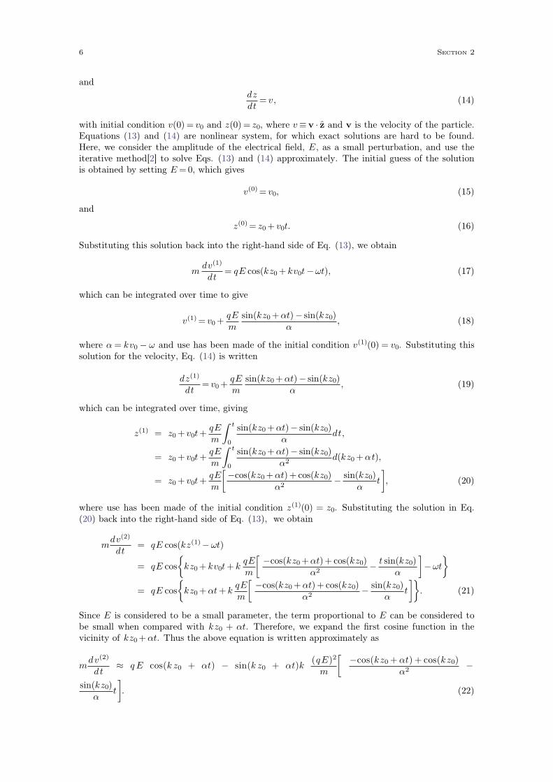
F1(vz)d vz = 1+ i. Equa-tion (77) with the initial condition Eq. (78) was solved numerically to obtain the time evolutionof F1 (the code is in /home/yj/project/landau_damping/). Figure 7 compares the velocity dis-tribution function at t = 0 with that at t = 40, which shows that the distribution functiondevelops �ne structures in velocity space.

Self-consistent-field linear simulation of Landau damping 13

-1-0.8-0.6-0.4-0.2

0 0.2 0.4 0.6 0.8

1

-4 -3 -2 -1 0 1 2 3 4 5v/vt

Re(f(0,v))Re(f(t,v))

-1-0.8-0.6-0.4-0.2

0 0.2 0.4 0.6 0.8

1

-4 -3 -2 -1 0 1 2 3 4 5v/vt

Im(f(0,v))Im(f(t,v))

Figure 7. Comparison of F1 at t = 0 and t!p = 40. (a) real part; (b) imaginary part. Other parameterskvt/!p= 0.5.

It is ready to realize that the �ne velocity space structures are partially due to the �rst termon the right-hand side of Eq. (77). When only this term is retained, Eq. (77) is written

@F1@t

=¡i�kvt!p

�vz F1; (79)

which has the dispersion relation

!=

�kvt!p

�vz; (80)

which indicates that Eq. (79) has di�erent eigenfrequencies for di�erent points in velocity space.Thus, an initially rather smooth velocity distribution function will become not so smooth aftersome time due to the distribution function oscillate with different frequencies at differentvelocity points. This is the so-called �phase mixing�. It is obvious that, after some time, thephase mixing will make the velocity distribution function F1(vz) rather messy, which poses agreat challenge to the numerical resolution of F1(vz). Given a �xed velocity grids, the numericalresults will become inaccurate when the grids is not �ne enough to resolve the �ne structures ofvelocity distribution.

Note that the electric �eld is related to the integration of F1, i.e.

E1=1ik

q"0

Z¡1

1F1 dvz (81)

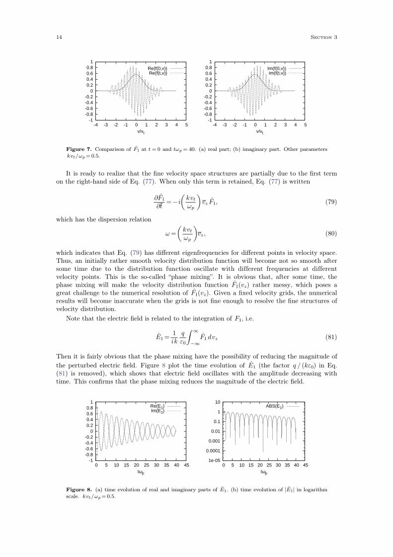
Then it is fairly obvious that the phase mixing have the possibility of reducing the magnitude ofthe perturbed electric �eld. Figure 8 plot the time evolution of E1 (the factor q / (k"0) in Eq.(81) is removed), which shows that electric �eld oscillates with the amplitude decreasing withtime. This con�rms that the phase mixing reduces the magnitude of the electric �eld.

-1-0.8-0.6-0.4-0.2

0 0.2 0.4 0.6 0.8

1

0 5 10 15 20 25 30 35 40 45tωp

Re(E1)Im(E1)

1e-05

0.0001

0.001

0.01

0.1

1

10

0 5 10 15 20 25 30 35 40 45tωp

ABS(E1)

Figure 8. (a) time evolution of real and imaginary parts of E1. (b) time evolution of jE1j in logarithmscale. kvt/!p= 0.5.

14 Section 3

3.4 Comparison with linear analytical theoryNext, we compare the numerical results with the electron plasma wave dispersion relation, whichis given by[1]

1+ 2

�!pkvt

�2

[1+ �Z(�)] = 0; (82)

where � =!/kvt, vt= 2Te/me

p, and

Z(�)=1

�p

ZC

e¡z2

z¡ �dz; (83)

is the plasma dispersion function. The plasma dispersion function can be written as

Z(�) = i �p

exp(¡�2)erfc(¡i�); (84)

where erfc is the complementary error function of imaginary argument, which is implemented inWolfram Mathematica. By using FindRoot function of Wolfram Mathematica, the equation (82)can be easily solved numerically to �nd the root. For the parameter used in the simulation kvt/!p= 0.5, Findroot gives � = 2.4508¡ i0.0725. From this, we obtain !/!p= �kvt/!p = 1.2254¡i0.0362.

The oscillation frequency of the electric �eld can be estimated by counting the peaks in Fig.8, from which we obtain !r / !p = 1.226, which agrees the theoretic value 1.2254 given above.Figure 8 shows that the amplitude of the electric �led decreases exponentially with time. Figure9 compares the theoretic growth rate with the simulation results, which also shows good agree-ment with each other.

-10-9-8-7-6-5-4-3-2-1 0 1

0 5 10 15 20 25 30 35 40 45tωp

ln|E1|theory

Figure 9. Comparison of the damping rate given by Eq. (82) ( /!p = ¡0.0362) with the simulationresults for the parameterkvt/!p= 0.5.

In the weak growth rate approximation, the real frequency of electron plasma wave is givenby

!r2=!p

2+3

2k2vt

2; (85)

For the numerical case given here, kvt /!p = 0.5. Using this in Eq. (85), we obtain !r / !p =1.173, which roughly agrees with the exact value !r/!p= 1.2254.

In the weak growth rate approximation, the growth rate is given by Eq. (45), i.e.,

=�!!p

2

2jk jk1n0

�df0(v)dv

�v=!/k

; (86)

Using this, we obtain

=�!!p

2

2k jk j1n0

�n0

vt �p exp

�¡v

2

vt2

��¡2vvt2

��v=!/k

=�!!p

2

2k2

�1

vt �p exp

�¡ !2

k2 vt2

��¡ 2!

kvt2

��: (87)

Self-consistent-field linear simulation of Landau damping 15

From this, we obtain

!p

= �p !p

kvt

"exp

¡ !r

2/!p2

k2vt2/!p

2

! ¡ !r

2/!p2

k2 vt2/!p

2

!#: (88)

Using !/!p= 1.225 in Eq. (88), we obtain /!p=¡0.0524, which roughly agrees with the exactvalue /!p = ¡0.0362 obtained above. Note that if we used ! � !p, instead of the exact fre-quency ! = 1.225!p, then Eq. (88) would give /!p = ¡0.259, which is almost one order largerthan the exact value /!p=¡0.036. This highlights the inaccuracy of the approximate formulawe encounter in textbooks[1], where !=!p is used to estimate the damping rate.

Figure 10 compares the exact numerical solution of the dispersion relation (82) with theapproximate solution given by Eqs. (85) and (88). The results indicate that the approximategrowth rate give by Eq. (88) is much lower than than the exact value for kvt/!pe> 1.

0 1 2 3 40

2

4

6

8

(kvt/ω

pe)2

(ωr/ω

pe)2

ExactApproximate

0 1 2 3 4−2

−1.5

−1

−0.5

0

(kvt/ω

pe)2

γ/ω

pe

ExactApproximate

Figure 10. Comparision of the exact numerical solution of the dispersion relation (82) with the approxi-mate solution given by Eqs. (85) and (88). Numerical calculation uses the Matlab implementation of theerror function of imaginary argument by Marcel Leutenegger (January 2008). The root of the dispersionequation is found by using �fsolve� of Matlab.

3.5 On the consrvation of particle numberIn the above, we see that the integration j

R¡11

F1dvz j decreases with time, which seems to beinconsistent with the conservation of particle number. Note the spatial dependence of the per-turbed distribution function is eikz, i.e., the perturbed distribution function is given by F1e

ikz,the real part of which corresponds to the physical distribution function, i.e., F1(t; vz; z) = A(t;

v)cos(kz + �), where A = jF1j and � is the angle of F1 on the complex plane. The particlenumber for the distribution function F1 in a region of the wave length 2�/k is given by

N =

Z0

2�/kZ¡1

1F1dvz dz

=

Z0

2�/k

dz

Z¡1

1A(t; v)cos(kz+ a)dvz

=

Z¡1

1A(t; v)

�Z0

2�/k

dz cos(kz+�)

�dvz (89)

Note that the term in the parenthesises is zero. Therefore the above expression is always zero nomatter what value the integration

R¡11

F1dvz is . Thus the number of particles is conserved inthis case.

4 Two-stream instabilityIn Sec. 3, the equilibrium velocity distribution of electrons is chosen to be Maxwellian, where wesee that perturbations are damped, which is the well-known Landau damping. In this section,we investigate a case where perturbation grows, instead of being damped. Consider an equilib-rium distribution function consisting of two counter-propagating Maxwellian beams of meanspeed vb and thermal spread vt, i.e.,

F0(vz) =n02

�1

vt �p exp

�¡(vz¡ vb)

2

vt2

�+

1

vt �p exp

�¡(vz+ vb)2

vt2

��: (90)

16 Section 4

Then @F0/@vz is written

@F0@vz

=n02

�1

vt �p exp

�¡ (vz ¡ vb)2

vt2

��¡2 (vz ¡ vb)

vt2

�+

1

vt �p exp

�¡ (vz+ vb)2

vt2

��¡

2 (vz+ vb)

vt2

��(91)

Using the same code discussed in Sec. 3, I solve Equation (74) with @F0/@vz given by Eq. (91)and the initial perturbation given by Eq. (77). Figure 11 plots the equilibrium distribution func-tion with vb/vt=4.

0

0.05

0.1

0.15

0.2

0.25

0.3

-8 -6 -4 -2 0 2 4 6 8v/vt

Figure 11. Equilibrium distribution function given by Eq. (90) with vb/vt=4.

Figure 12 plots the time evolution of the perturbed electric �eld, which shows the the electric�eld grows exponentially in time and thus corresponds to an instability. This instability is calledtwo-stream instability since it happens in the system with two opposite electron beams.

-6-4-2 0 2 4 6 8

10 12 14

0 10 20 30 40 50 60 70 80 90tωp

ln|E1|theory

Figure 12. Comparison of the simulation results with analytical growth rate given by Eq. (92). Theparameters are kvt/!p= 0.05 and vb/vt=4.

In Fig. 12, the simulation results are also compared with the analytical results in the coldbeam approximation (vt! 0), which is given by equation (8.1.35) in Gurnett's book[1], i.e.,

!p

= 1+4k2vb

2

!p2

s¡

1+

k2vb2

!p2

!vuut ; (92)

To make the simulation result able to be compared with the results in the cold beam approxi-mation, the thermal velocity of the beam has been chosen to be a small number kvt/!p = 0.05.The results in Fig. 12 shows that the simulation results agree with the analytical results. Thesmall discrepancy can be attributed to that equation (92) was derived by assuming the electrondistribution function is a Dirac � function while in the simulation, the distribution function is aMaxwellian distribution with small a thermal spread (kvt / !p = 0.05). Also note that in thiscase, the approximate phase velocity of the electron plasma wave is vp = !p / k = 20vt and thebeam velocity vb = 4vt. Thus, the distribution function is very small at the phase velocity.Therefore the Landau damping in this case is neglectably small. In fact, equation (92) wasderived in the �uid mode in which the Landau damping is not included.

Two-stream instability 17

-2.5e+06-2e+06

-1.5e+06-1e+06

-500000 0

500000 1e+06

1.5e+06 2e+06

2.5e+06 3e+06

-8 -6 -4 -2 0 2 4 6 8 10v/vt

Re(f(0,v))Re(f(t,v))

-2.5e+06-2e+06

-1.5e+06-1e+06

-500000 0

500000 1e+06

1.5e+06 2e+06

2.5e+06 3e+06

-8 -6 -4 -2 0 2 4 6 8 10v/vt

Im(f(0,v))Im(f(t,v))

Figure 13. Real part (a) and imaginary part (b) of the perturbed distribution function F1 at t!p= 80.The parameters are kvt/!p= 0.05 and vb/vt=4.

5 tmp��to be deleted����As is given in the wikipedia, the ponderomotive force is a nonlinear force that acharged particle experiences in an inhomogeneous oscillating electromagnetic �eld. The pondero-motive force Fp is expressed by

Fp=¡e2

4m!2rE2; (93)

where e is the electrical charge of the particle, m is the mass of the particle, E is the amplitudeof the inhomogeneous oscillating electric field (at low enough amplitudes the magnetic fieldexerts very little force), ! is the angular frequency of oscillation of the �eld. to be continued�

"(k; !)= 1+e2

"0mek

ZC

@f0/@v!¡ kv dv=0

1¡ 2 e2

"0mekn0

vt �p 1

kvt

ZC

exp(¡t2)� ¡ t tdt=0

Z(�) =2ie¡�2

Z¡1

i�

e¡t2dt: (94)

Z(�)= i �p

w(�); (95)

where w(�) is Faddeeva's function, which is de�ned by

w(�)= exp(¡�2)erfc(¡i�): (96)

Z(�) = i �p

exp(¡�2)erfc(¡i�)

= i �p

exp(¡�2) 2

�p

Z¡i�

1e¡t

2dt

= 2i exp(¡�2)Z¡1

i�

e¡t2dt (97)

Bibliography[1] D. A. Gurnett and A. Bhattacharjee. Introduction to plasma physics : with space and laboratory applica-

tions. Cambridge University Press, Cambridge, UK, 2004.

18 Section

[2] E.J. Hinch. Perturbation methods. Cambridge University Press, 1991.[3] Dwight R. Nicholson. Introduction to Plasma Theory. John Wiley & Sons, 1983.[4] T. H. Stix. Waves in plasma. American Institute of Physics, New York, 1992.

Bibliography 19