NOTES ON GENERAL RELATIVITY (GR) AND GRAVITY

ERNEST YEUNG

Abstract. These are notes on General Relativity (GR) and Gravity.

As of March 23, 2015, I find that the Central Lectures given by Dr. Frederic P. Schuller for the WE Heraeus International

Winter School to be, unequivocally, the best, most lucid, and well-constructed lecture series on General Relativity and

Gravity. Instead of reinventing the wheel, I write these notes to build upon and supplement the video lectures and tutorials

already created by them. This includes my corrections, comments, relations to other aspects of theoretical physics, and code

implementing calculations in GR.

It should be noted that for symbolic computation, I heavily use the SageManifolds v.0.7 package for Sage Math. My goal

in this area is this: we see a concept or idea from GR and we go from the equation on the blackboard or textbook and into

(Python/Sage Math) code that immediately computes a calculation.

I keep these notes available online, openly accessible, and free for anyone, anytime (with your (financial) help and con-

tribution at Tilt/Open, which is a subscription service). I want to keep these notes openly accessible because I want to

encourage anyone to freely edit, copy, and make their own notes in the spirit of open-source software.

I continuously update these notes and post them here ernestyalumni.wordpress.com

The stated goal of the WE Heraeus International Winter School on Gravity and Light is to take the student from an

introduction to the research frontier (cf. http://www.gravity-and-light.org/lectures). I want to get myself and other

students or ambitious non-academic (maybe he or she is a working professional who had studied physics before in college,

went to work in another field, maybe even, gasp, investment banking or mobile app developer, but still is curious and

passionate about physics and want to contribute) equipped with all the tools available to do research, do calculations, to

design experiments or collect data. Again, we’re not here to reinvent the wheel. I’m not trying to make a General Relativity

appreciation class, but this is a serious attempt towards training to do research.

Part 1. WE Heraeus International Winter School on Gravity and Light 2

Introduction (from EY) 2

1. Lecture 1: Topology 2

Topology Tutorial Sheet 4

2. Lecture 2: Topological Manifolds 4

Tutorial Topological manifolds 5

3. 7

4. Lecture 4: Differentiable Manifolds 7

Tutorial 4 Differentiable Manifolds 10

5. Lecture 5: Tangent Spaces 12

6. 16

7. Lecture 7: Connections 16

8. Lecture 8: Parallel Transport & Curvature (International Winter School on Gravity and Light 2015) 20

Tutorial 8 Parallel transport & Curvature 21

9. Lecture 9: Newtonian spacetime is curved! 23

10. Lecture 10: Metric Manifolds 26

Date: 23 mars 2015.

1991 Mathematics Subject Classification. General Relativity.

Key words and phrases. General Relativity, Gravity, Differential Geometry, Manifolds, Integration, MIT OCW, education, mathematics,

physics.

I write notes, review papers, and code and make calculations for physics, math, and engineering to help with education and research. With

your support, we can keep education and research material available online, openly accessible, and free for anyone, anytime. If you like what

I’m trying to do for physics education research, please go to my Tilt/Open crowdfunding campaign, read the mission statement, share the page,

and contribute financially if you can. ernestyalumni.tilt.com .

1

11. Symmetry 31

12. Integration 34

13. Lecture 13: Relativistic spacetime 37

14. Lecture 14: Matter 40

15. Lecture 15: Einstein gravity 43

Tutorial 13 Schwarzschild Spacetime 47

16. 48

17. 48

18. 48

19. 48

20. 48

21. 48

22. Lecture 22: Black Holes 48

Part 2. Special Relativity 51

References 51

Contents

Part 1. WE Heraeus International Winter School on Gravity and Light

Introduction (from EY)

The International Winter School on Gravity and Light held central lectures given by Dr. Frederic P. Schuller. These

lectures on General Relativity and Gravity are unequivocally and undeniably, the best and most lucid and well-constructed

lecture series on General Relativity and Gravity. The mathematical foundation from topology and differential geometry

from which General Relativity arises from is solid, well-selected in rigor. The lectures themselves are well-thought out and

clearly explained.

Even more so, the International Winter School provided accompanying Tutorial Sessions for each of the lectures. I had

given up hopes in seeing this component of the learning process ever be put online so that anyone and everyone in the world

could learn through the Tutorial process as well. I was afraid that nobody would understand how the Tutorial or “Office

Hours” session was important for students to digest and comprehend and work out-doing exercises-the material presented

in the lectures. This International Winter School gets it and shows how online education has to be done, to do it in an

excellent manner, moving forward.

For anyone who is serious about learning General Relativity and Gravity, I would simply point to these video lectures and

tutorials.

What I want to do is to build upon the material presented in this International Winter School. Why it’s important to

me, and to the students and practicing researchers out there, is that the material presented takes the student from an

introduction to the research frontier. That is the stated goal of the International Winter School. I want to dig into and

help contribute to the cutting edge in research and this entire program with lectures and tutorials appears to be the most

direct and sensible route directly to being able to do research in General Relativity and Gravity. -EY 20150323

1. Lecture 1: Topology

1.1. Lecture 1: Topological Spaces.

Definition 1. Let M be a set.

A topology O is a subset O ⊆ P(M), P(M) power set of M : set of all subsets of M . satisfying

(i) ∅ ∈ O, M ∈ O2

(ii) U ∈ O, V ∈ O =⇒ U⋂V ∈ O

(iii) Uα ∈ O, α ∈ A =⇒(⋃

α∈A Uα)∈ O

O utterly useless

Definition 2. Ostandard ⊆ P(Rd)

EY : 20150524

I’ll fill in the proof that Ostandard is a topology.

Proof. ∅ ∈ Ostandard

since ∀ p ∈ ∅, ∃ r ∈ R+: Br(p) ⊆ ∅ (i.e. satisfied “vacuously”)

Suppose U, V ∈ Ostandard.

Let p ∈ U⋂V . Then ∃ r1, r2 ∈ R+ s.t. Br1(p) ⊆ U

Br2(p) ⊆ V

Let r = min r1, r2.Clearly Br(p) ⊆ U and Br(p) ⊆ V . Then Br(p) ⊆ U

⋂V . So U

⋂V ∈ Ostandard.

Suppose, Uα ∈ Ostandard, ∀α ∈ A.

Let p ∈⋃α∈A Uα. Then p ∈ Uα for at least 1 α ∈ A.

∃ rα ∈ R+ s.t. Brα(p) ⊆ Uα ⊆⋃α∈A Uα. So

⋃α∈A Uα ∈ Ostandard

1.2. 2. Continuous maps.

1.3. 3. Composition of continuous maps.

1.4. 4. Inheriting a topology. EY : 20150524

I’ll fill in the proof that given f continuous (cont.), then the restriction of f onto a subspace S is cont. If you want a

reference, check out Klaus Janich [2, pp. 13, Ch. 1 Fundamental Concepts, Sec. Continuous Maps]

If cont. f : M → N , S ⊆M , then f |S cont.

Proof. Let open V ⊆ N , i.e. V ∈ ON i.e. V in the topology ON of N .

f |−1S (V ) = m ∈M | f |S (m) ∈ V

Now f−1(V ) = m ∈M |f(m) ∈ V .So f−1(V )

⋂S = f |−1

S (V )

Now f cont. So f−1(V ) ∈ ON .

and recall OS | := U⋂S|U ∈ OM.

so f−1(V )⋂S = f |−1

S (V ) ∈ OS i.e. f |−1S (V ) open.

=⇒ f |S cont.

3

Topology Tutorial Sheet

filename : main.pdf

The WE-Heraeus International Winter School on Gravity and Light: Topology

EY : 20150524

What I won’t do here is retype up the solutions presented in the Tutorial (cf. https://youtu.be/_XkhZQ-hNLs): the

presenter did a very good job. If someone wants to type up the solutions and copy and paste it onto this LaTeX file, in

the spirit of open-source collaboration, I would encourage this effort.

Instead, what I want to encourage is the use of as much CAS (Computer Algebra System) and symbolic and numerical

computation because, first, we’re in the 21st century, second, to set the stage for further applications in research. I use

Python and Sage Math alot, mostly because they are open-source software (OSS) and fun to use. Also note that the

structure of Sage Math modules matches closely to Category Theory.

In checking whether a set is a topology, I found it strange that there wasn’t already a function in Sage Math to check each

of the axioms. So I wrote my own; see my code snippet, which you can copy, paste, edit freely in the spirit of OSS here,

titled topology.sage:

gist github ernestyalumni topology.sage

Download topology.sage

Loading topology.sage, after changing into (with the usual Linux terminal commands, cd, ls) by

sage: load(‘‘topology.sage’’)

Exercise 2: Topologies on a simple set.

Question Does O1 := . . . constitute a topology . . . ?.

Solution: Yes, since we check by typing in the following commands in Sage Math:

emptyset in O_1

Axiom2check(O_1) # True

Axiom3check(O_1) # True

Question What about O2 . . . ?.

Solution: No since the 3rd. axiom fails, as can be checked by typing in the following commands in Sage Math:

emptyset in O_2

Axiom2check(O_2) # True

Axiom3check(O_2) # False

2. Lecture 2: Topological Manifolds

Lecture 2: Manifolds. Topological spaces: ∃ so man that mathematicians cannot even classify them.

For spacetime physics, we may focus on topological spaces (M,O) that can be charted, analogously to how the surface of

the earth is charted in an atlas.

2.1. Topological manifolds.

Definition 3. A topological space (M,O) is called a d-dimensional topological method if

∀ p ∈M : ∃U ∈ O, U 3 p : ∃x : U ⊆M → x(U) ⊆ Rd (M,O), (Rd,Ostd)

(i) x invertible :

x−1 : x(U)→ U

4

(ii) x continuous

(iii) x−1 continuous

2.2. Terminology.

2.3. 3. Chart transition maps. Imagine 2 charts (U, x) and (V, y) with overlapping regions.

2.4. 4. Manifold philosophy. Often it is desirable (or indeed the way) to define properties (“continuity”) of real-world

object (“R γ−→ M”) by judging suitable coordinates not on the “real-world” object itself, but on a chart-representation of

that real world object.

EY’s add-ons. This lecture gives me a good excuse to review Topology and Topological Manifolds from a mathemati-

cian’s point of view. I find John M. Lee’s Introduction to Topological Manifolds book good because it’s elementary

and thorough and it’s fairly recent (2010) so it’s up to date [3]. See my notes and solutions for the book; it’s a file ti-

tled LeeJM_IntroTopManifolds_sol.pdf of which I’ll try to keep the pdf and LaTeX file available for download on my

ernestyalumni Google Drive (so try to search for it on Google).

Tutorial Topological manifolds

filename: Sheet_1.2.pdf

Exercise 4: Before the invention of the wheel.

Another one-dimensional topological manifold. Another one?

Consider set F 1 := (m,n) ∈ R2|m4 + n4 = 1, equipped with subset topology Ostd|F 1

Question x : F 1 → R is what?.

Solution . EY : 20150525 The tutorial video https://youtu.be/ghfEQ3u_B6g is really good and this solution is how I’d

write it, but it’s really the same (I needed the practice).

x : F 1 → R

(m,n) 7→ m

If m = 0, n4 = 1 so n = ±1 so it’s not injective.

Let the closed n-dim. upper half-space Hn ⊆ R1. Then

Hn = (x1 . . . xn) ∈ Rn|xn ≥ 0

intHn = (x1 . . . xn) ∈ Rn|xn > 0

−Hn = (x1 . . . xn) ∈ Rn|xn ≤ 0

−intHn = (x1 . . . xn) ∈ Rn|xn < 0

Question This map x may be made injective by restricting its domain to either of 2 maximal open subsets of F 1.

Which ones?.

Solution .

LetU+ = F 1 ∩ intH2

U− = F 1 ∩ −intH2

5

Look at

x4 = 1− n4

=⇒x = ±(1− n4)1/4

Then for

x−1+ : (−1, 1) ⊆ R→ U+

m 7→ (m, (1−m4)1/4)

x−1− : (−1, 1) ⊆ R→ U−

m 7→ (m,−(1−m4)1/4)

x+,x− injective (since left inverse exists).

Question Construct injective y.

Solution .

Let

V+ = F 1 ∩ intH1

V− = F 1 ∩ −intH1

Then

y+ : V+ → (−1, 1) ⊆ R

(m,n) 7→ n

y− : V− → (−1, 1) ⊆ R

(m,n) 7→ n

Question Construct inverse y−1. Solution .

For

y−1+ : (−1, 1) ⊆ R→ V+

n 7→ ((1− n4)1/4, n)

y−1− : (−1, 1) ⊆ R→ V−

n 7→ (−(1− n4)1/4, n)

y+,y− injective (since left inverse exists).

Note (−1, 0) /∈ U+, U−

(1, 0) /∈ U+, U−

and

(0, 1) /∈ V+, V−

(0,−1) /∈ V+, V−

Question construct transition map x y−1.

Solution .

6

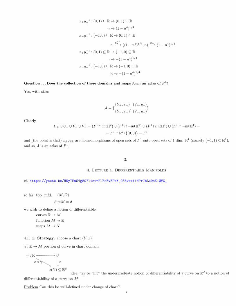
x+y−1+ : (0, 1) ⊆ R→ (0, 1) ⊆ R

n 7→ (1− n4)1/4

x−y−1+ : (−1, 0) ⊆ R→ (0, 1) ⊆ R

ny−1+−−→ ((1− n4)1/4, n)

x−−−→ (1− n4)1/4

x+y−1− : (0, 1) ⊆ R→ (−1, 0) ⊆ R

n 7→ −(1− n4)1/4

x−y−1− : (−1, 0) ⊆ R→ (−1, 0) ⊆ R

n 7→ −(1− n4)1/4

Question . . . Does the collection of these domains and maps form an atlas of F 1?.

Yes, with atlas

A = (U+, x+)

(U−, x−),

(V+, y+)

(V−, y−)

Clearly

U+ ∪ U− ∪ V+ ∪ V− = (F 1 ∩ intH2) ∪ (F 1 ∩ −intH2) ∪ (F 1 ∩ intH1) ∪ (F 1 ∩ −intH1) =

= F 1 ∩ R2\(0, 0) = F 1

and (the point is that) x±, y± are homeomorphisms of open sets of F 1 onto open sets of 1 dim. R1 (namely (−1, 1) ⊆ R1),

and so A is an atlas of F 1.

3.

4. Lecture 4: Differentiable Manifolds

cf. https://youtu.be/HSyTEwS4g80?list=PLFeEvEPtX_0S6vxxiiNPrJbLu9aK1UVC_

so far: top. mfd. (M,O)

dimM = d

we wish to define a notion of differentiable

curves R→M

function M → Rmaps M → N

4.1. 1. Strategy. choose a chart (U, x)

γ : R→M portion of curve in chart domain

γ : R U

x(U) ⊆ Rd

x γ x

idea. try to “lift” the undergraduate notion of differentiability of a curve on Rd to a notion of

differentiability of a curve on M

Problem Can this be well-defined under change of chart?7

y(U ∩ V ) ⊆ Rd

γ : R U ∩ V 6= ∅

x(U ∩ V ) ⊆ Rd

x γ

y γ

x

y

y x−1

x γ undergraduate differentiable (“as a map R→ Rd”)

y γ︸︷︷︸maybe only continuous, but not undergraduate differentiable

= (

Rd→Rd︷ ︸︸ ︷y x−1)︸ ︷︷ ︸

continuous

(

R→Rd︷ ︸︸ ︷x γ )︸ ︷︷ ︸

undergrad differentiable

= y (x−1 x) γ

At first sight, strategy does not work out.

4.2. 2. Compatible charts. In section 1, we used any imaginable charts on the top. mfd. (M,O).

To emphasize this, we may say that we took U and V from the maximal atlas A of (M,O).

Definition 4. Two charts (U, x) and (V, y) of a top. mfd. are called `-compatible if either

(a) U ∩ V = ∅ or

(b) U ∩ V 6= ∅

chart transition maps have undergraduate ` property.

EY : 20151109 e.g. since Rd → Rd, can use undergradate ` property such as continuity or differentiability.

y x−1 : x(U ∩ V ) ⊆ Rd → y(U ∩ V ) ⊆ Rd

x y−1 : y(U ∩ V ) ⊆ Rd → x(U ∩ V ) ⊆ Rd

Philosophy:

Definition 5. An atlas A‘ is a `-compatible atlas if any two charts in A` are `-compatible.

Definition 6. A `-manifold is a triple ( M,O︸ ︷︷ ︸top. mfd.

,A`) A` ⊆ Amaximal

` undergraduate `

C0 C0(Rd → Rd) = continuous maps w.r.t. OC1 C1(Rd → Rd) = differentiable (once) and is continuous

Ck k-times continuously differentiable

Dk k-times differentiable...

C∞ C∞(Rd → Rd)

⊇

Cω ∃ multi-dim. Taylor exp.

C∞ satisfy Cauchy-Riemann equations, pair-wise

EY : 20151109 Schuller says: Ck is easy to work with because you can judge k-times cont. differentiability from existence

of all partial derivatives and their continuity. There are examples of maps that partial derivatives exist but are not Dk,

k-times differentiable.8

Theorem 1 (Whitney). Any Ck≥1-atlas, ACk≥1 of a topological manifold contains a C∞-atlas.

Thus we may w.l.o.g. always consider C∞-manifolds, “smooth manifolds”, unless we wish to define Taylor expandibility/-

complex differentiability . . .

EY : 20151109 Hassler Whitney 1

Definition 7. A smooth manifold ( M,O︸ ︷︷ ︸top. mfd.

, A︸︷︷︸C∞−atlas

)

R M

Rd

γ

x γx

EY: 20151109 Schuller was explaining that the trajectory is real in M ; the coordinate maps to

obtain coordinates is x γ

4.3. 4. Diffeomorphisms. Mφ−→ N

If M,N are naked sets, the structure preserving maps are the bijections (invertible maps).

e.g. 1, 2, 3 → a, b

Definition 8. M ∼=set N (set-theoretically) isomorphic if ∃ bijection φ : M → N

Examples. N ∼=set ZN ∼=set Q (EY: 20151109 Schuller says from diagonal counting)

N∼=setR

Now (M,OM ) ∼=top (N,ON ) (topl.) isomorphic = “homeomorphic” ∃ bijection φ : M → N

φ, φ−1 are continuous.

(V,+, ·) ∼=vec (W,+w, ·w) (EY: 20151109 vector space isomorphism) if

∃ bijection φ : V →W linearly

finally

Definition 9. Two C∞-manifolds

(M,OM ,AM ) and (N,ON ,AN ) are said to be diffeomorphic if ∃ bijection φ : M → N s.t.

φ : M → N

φ−1 : N →M

are both C∞-maps

Rd Re

M ⊇ U V ⊆ N

Rd Re

y φ x−1

x

φ

x

yφx−1

undergraduate C∞

C∞

y

y

1http://mathoverflow.net/questions/8789/can-every-manifold-be-given-an-analytic-structure

9

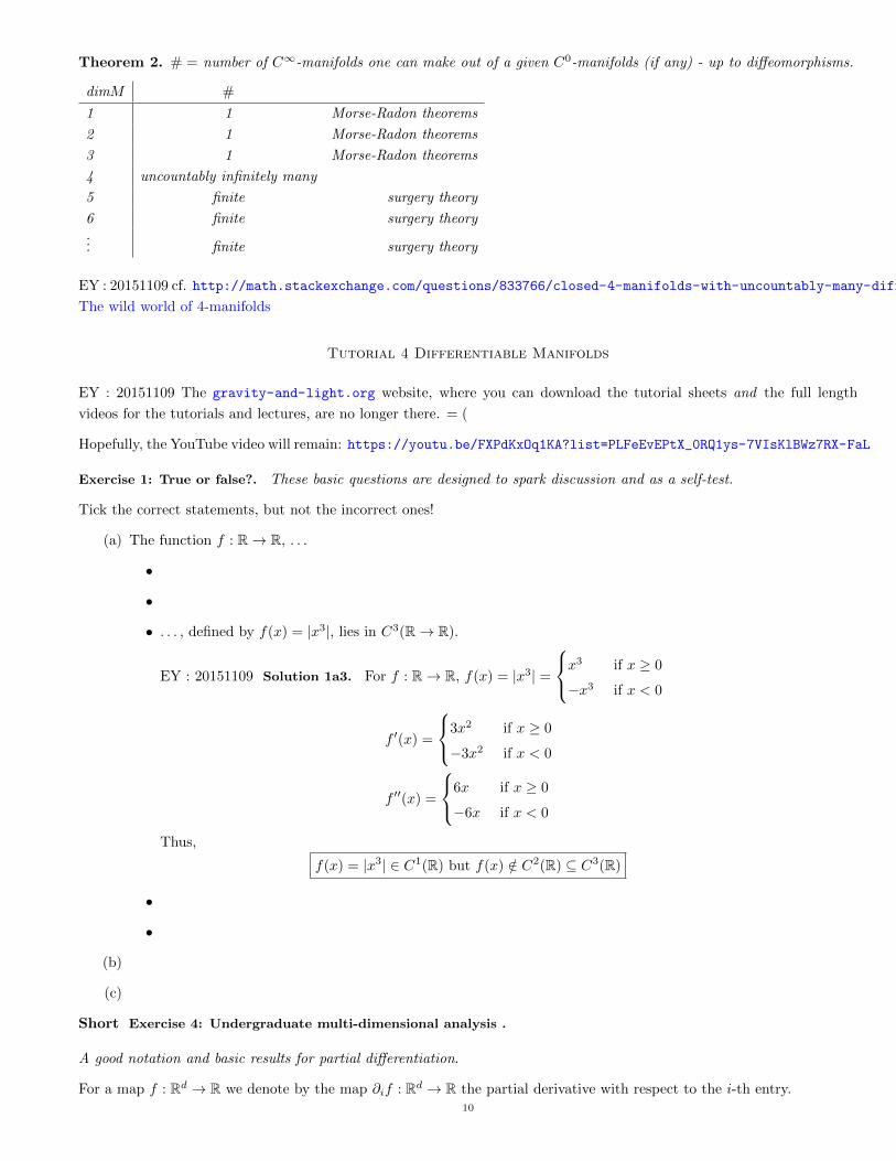
Theorem 2. # = number of C∞-manifolds one can make out of a given C0-manifolds (if any) - up to diffeomorphisms.

dimM #

1 1 Morse-Radon theorems

2 1 Morse-Radon theorems

3 1 Morse-Radon theorems

4 uncountably infinitely many

5 finite surgery theory

6 finite surgery theory... finite surgery theory

EY : 20151109 cf. http://math.stackexchange.com/questions/833766/closed-4-manifolds-with-uncountably-many-differentiable-structures

The wild world of 4-manifolds

Tutorial 4 Differentiable Manifolds

EY : 20151109 The gravity-and-light.org website, where you can download the tutorial sheets and the full length

videos for the tutorials and lectures, are no longer there. = (

Hopefully, the YouTube video will remain: https://youtu.be/FXPdKxOq1KA?list=PLFeEvEPtX_0RQ1ys-7VIsKlBWz7RX-FaL

Exercise 1: True or false?. These basic questions are designed to spark discussion and as a self-test.

Tick the correct statements, but not the incorrect ones!

(a) The function f : R→ R, . . .

•

•

• . . . , defined by f(x) = |x3|, lies in C3(R→ R).

EY : 20151109 Solution 1a3. For f : R→ R, f(x) = |x3| =

x3 if x ≥ 0

−x3 if x < 0

f ′(x) =

3x2 if x ≥ 0

−3x2 if x < 0

f ′′(x) =

6x if x ≥ 0

−6x if x < 0

Thus,

f(x) = |x3| ∈ C1(R) but f(x) /∈ C2(R) ⊆ C3(R)

•

•

(b)

(c)

Short Exercise 4: Undergraduate multi-dimensional analysis .

A good notation and basic results for partial differentiation.

For a map f : Rd → R we denote by the map ∂if : Rd → R the partial derivative with respect to the i-th entry.10

Question :. Given a function

f : R3 → R; (α, β, δ) 7→ f(α, β, δ) := α3β2 + β2δ + δ

calculate the values of the following derivatives:

Solution :.

• (∂2f)(x, y, z) =

• (∂1f)(, , ∗) =

• (∂1∂2f)(a, b, c) =

• (∂23f)(299, 1222, 0) =

EY: 20151110

For f(α, β, δ) := α3β2 + β2δ + δ, or f(x, y, z) = x3y2 + y2z + z,

(∂2f) = 2(x3y + yz)

(∂1f) = 3x2y2

(∂1∂2f) = 6x2y

(∂23f) = 0

and so

• (∂2f)(x, y, z) = 2(x3y + yz)

• (∂1f)(, , ∗) = 322

• (∂1∂2f)(a, b, c) = 6a2b

• (∂23f)(299, 1222, 0) = 0

Exercise 5: Differentiability on a manifold.

How to deal with functions and curves in a chart

Let (M,O,A) be a smooth d-dimensional manifold. Consider a chart (U, x) of the atlas A together with a smooth curve

γ : R→ U and a smooth function f : U → R on the domain U of the chart.

Question :. Draw a commutative diagram containing the chart domain, chart map, function, curveand the respective

representatives of the function and the curve in the chart.

Solution :.

R U Rd

R

γ

x γ

x−1

(f x−1)f

x τ ∈ R p ∈ U x(p) = (x γ)(τ) ∈ Rd

f(p) ∈ R

γ

x γ

x−1

(f x−1)f

x

Question :. Consider, for d = 2,

(x γ)(λ) := (cos (λ), sin (λ)) and (f x−1)((x, y)) := x2 + y2

Using the chain rule, calculate

(f γ)′(λ)11

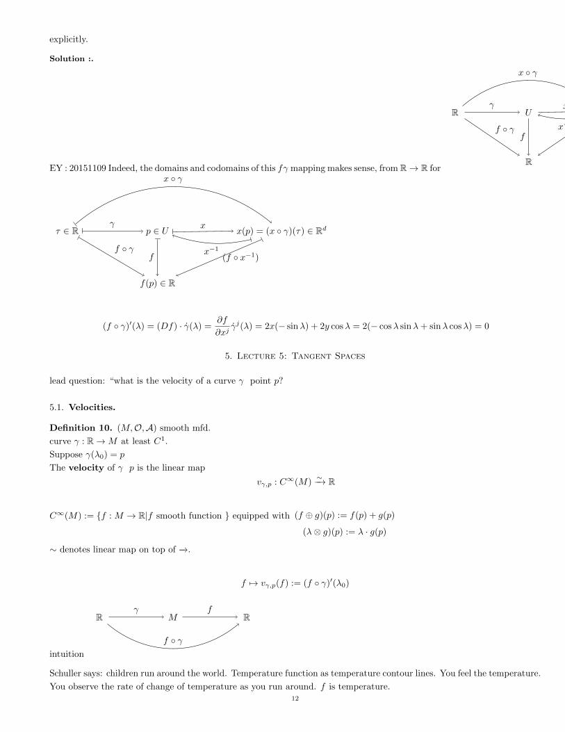
explicitly.

Solution :.

EY : 20151109 Indeed, the domains and codomains of this fγ mapping makes sense, from R→ R for

R U Rd

R

γ

x γ

f γ x−1

(f x−1)f

x

τ ∈ R p ∈ U x(p) = (x γ)(τ) ∈ Rd

f(p) ∈ R

γ

x γ

f γ x−1

(f x−1)f

x

(f γ)′(λ) = (Df) · γ(λ) =∂f

∂xjγj(λ) = 2x(− sinλ) + 2y cosλ = 2(− cosλ sinλ+ sinλ cosλ) = 0

5. Lecture 5: Tangent Spaces

lead question: “what is the velocity of a curve γ point p?

5.1. Velocities.

Definition 10. (M,O,A) smooth mfd.

curve γ : R→M at least C1.

Suppose γ(λ0) = p

The velocity of γ p is the linear map

vγ,p : C∞(M)∼−→ R

C∞(M) := f : M → R|f smooth function equipped with (f ⊕ g)(p) := f(p) + g(p)

(λ⊗ g)(p) := λ · g(p)

∼ denotes linear map on top of −→.

f 7→ vγ,p(f) := (f γ)′(λ0)

intuition

R M Rγ

f γ

f

Schuller says: children run around the world. Temperature function as temperature contour lines. You feel the temperature.

You observe the rate of change of temperature as you run around. f is temperature.12

past: “ vi︸︷︷︸(∂if) = ( vi∂i︸︷︷︸vector

)f

5.2. Tangent vector space.

Definition 11. For each point p ∈Mdef the set “tangent space 6=0 M p “

TpM := vγ,p|γ smooth curves

picture:

rather M than (embedded) p TpM EY : 20151109 see https://youtu.be/pepU_7NJSGM?t=12m38s for the picture

Observation: TpM can be made into a vector space.

⊕ :TpM × TpM →

(vγ,p ⊕ vδ,p)( f︸︷︷︸∈C∞(M)

) := vγ,p(f) +R vδ,p(f)

:R× TpM → Hom(C∞(R),R)

(α vγ,p)(f) := α ·R vγ,p(f)

Remains to be shown that

(i) ∃σ curve : vγ,p ⊕ vδ,p = vσ,p

(ii) ∃ τ curve : α vγ,p = vτ,p

Claim: τ : R→M

7→ τ(λ) := γ(αλ+ λ0) = (γ µα)(λ)

where µα :R→ R

r 7→ α · r + λ0

, does the trick.

τ(0) = γ(λ0) = p

vτ,p := (f τ)′(0) = (f γ µα)′(0)

= (f γ)′(λ0) · α =

= α · vγ,p

Now for the sum:

vγ,p ⊕ vδ,p?= vσ,p

make a choice of chart ( U︸︷︷︸3p

, x) In cloud: ill definition alarm bells.

and define:

Claim:σ : R→M

σ(λ) := x−1((x γ)(λ0 + λ)︸ ︷︷ ︸R→Rd

+(x δ)(λ1 + λ)− (x γ)(λ0))

does the trick.

Proof. Since:

σx(0) = x−1((x γ)(λ0) + (x δ)(λ1)− (x γ)(λ0))

= δ(λ1) = p

13

Now:vσx,p(f) := (f σx)′(0) =

= ((f x−1)︸ ︷︷ ︸Rd→R

(x σx)︸ ︷︷ ︸R→Rd

)′(γ) = (x σx)′(0)︸ ︷︷ ︸(xγ)′(λ0)+(xδ)′(λ1)

·(∂i(f x−1)

)(x(σ(0)︸︷︷︸

p

)) =

= (x γ)′(λ0)(∂i(f x−1))(x(p)) + (x δ)(λ1)(∂i(f x−1))(x(p))

= (f γ)′(λ0) + (f δ)′(λ1) =

= vγ,p(f) + vδ,p(f) ∀ f ∈ C∞(M)

vγ,p ⊕ vδ,p = vσ,p

R M R

Rd

σ

x σx

f

f x−1

picture: (cf. https://youtu.be/pepU_7NJSGM?t=39m5s)

γ : R→M

δ : R→M

(γ⊕)(λ) := γ(λ) + δ(λ)

EY : 20151109 Schuller says adding trajectories is chart dependent, bad. Adding velocities is good.

5.3. Components of a vector wrt a chart.

Definition 12. Let (U, x) ∈ Asmooth.

Letγ : R→ U

γ(0) = p.

Calculatevγ,p(f) := (f γ)′(0) = ((f x−1)︸ ︷︷ ︸

Rd→R

(x γ)︸ ︷︷ ︸R→Rd

)′(0)

= (x γ)i′(0)︸ ︷︷ ︸

γix(0)

· (∂i(f x−1))(x(p))︸ ︷︷ ︸=:( ∂f

∂xi)p

think cloud f : M → R

= γix(0) ·(

∂

∂xi

)p

f ∀ f ∈ C∞(M)

∴ as a map.

vγ,p =︸︷︷︸use of chart

γix(0)︸ ︷︷ ︸“components of the velocity vγ,p”

(∂

∂xi

)︸ ︷︷ ︸

basis elements of the TpM wrt which the components need to be understood.“chart induced basis of TpM”

Picture: https://youtu.be/pepU_7NJSGM?t=1h16s14

5.4. 4. Chart-induced basis.

Definition 13. (U, x) ∈ Asmooth

the(∂∂x1

)p, . . . ,

(∂∂xd

)p∈ TpU ⊆ TpM

constitute a basis of TpU

Proof. remains: linearly independent

λi(

∂

∂xi

)p

!= 0

=⇒ λi(

∂

∂xi

)p

(xj) = λi∂i(xj x−1︸ ︷︷ ︸)(x(p)) =

= λiδ ji = λj j = 1, . . . , d

xj x−1 : Rd → R

(α1, . . . , αd) 7→ αj

in cloud: xj : U → R differentiable

Corollary 1. dimTpM = d = dimM

Terminology: X ∈ TpM → ∃ γ : R→M : X = vγ,p and

∃ X11 , . . . , X

d︸ ︷︷ ︸∈R

: X = Xi(∂∂xi

)p

5.5. 5. Change of vector components under a change of chart. 8 vector does not change under change of

chart.

Let (U, x) and (V, y) be overlapping charts and p ∈ U ∩ V .

Let X ∈ TpM

Xi(y) ·

(∂

∂yi

)p

=︸︷︷︸(V,y)

X =︸︷︷︸(U,x)

Xix

(∂

∂xi

)p

to study change of components formula:(∂

∂xi

)p

f = ∂i(f x−1)(x(p)) =

= ∂i((f y−1)︸ ︷︷ ︸Rd→R

(y x−1︸ ︷︷ ︸Rd→Rd

)(x(p))

= (∂i(yi x−1))(x(p)) · (∂j(f y−1))(y(p)) =

=

(∂yp

∂xi

)p

·(∂f

∂yj

)p

f

=⇒ Xi(x)

(∂yj

∂xi

)p

(∂

∂yj

)p

= Xj(y)

(∂

∂yj

)p

=⇒ Xj(y) =

(∂yj

∂xi

)p

Xi(x)

15

5.6. 6. Cotangent spaces. TpM = V

trivial (TpM)∗ := ϕ : TpM∼−→ R

Example: f ∈ C∞(M)

(df)p :TpM∼−→ R

X 7→ (df)p(X)

i.e. (df)p ∈ TpM∗

(df)p called the gradient of f p ∈M .

Calculate components of gradient w.r.t. chart-induced basis (U, x)

((df)p)j := (df)p

((∂

∂xj

)p

)

=

(∂f

∂xj

)p

= ∂j(f x−1)(x(p))

Theorem 3. Consider chart (U, x) =⇒ xi : U → R

Claim: (dx1)p, (dx2)p, . . . , (dx

d)p basis of T ∗pM

=⇒ In fact: dual basis:

(dxa)p

((∂

∂xb

)p

)=

(∂xa

∂xb

)p

= · · · = δab

5.7. 7. Change of components of a covector under a change of chart:

T ∗pM︸ ︷︷ ︸3ω

with ω(y)(dyj)p = ω = ω(x)i(dx

i)p

=⇒ ω(y)i =∂xj

∂yiω(x)j

6.

7. Lecture 7: Connections

∇Xf = Xf = (df)(X) but (not quite)

X : C∞(M)→ C∞(M)

df : Γ(TM)→ C∞(M)

∇X : C∞(M)→ C∞(M)

∇X : C∞(M) C∞(M)

∇X :TMp ⊗ T ∗Mq i.e.(

p

q

)tensor field

TMp ⊗ T ∗Mq i.e.(p

q

)tensor field

......

16

7.1. Directional derivatives of tensor fields. manifold with connection is quadruple (M,O,A,∇)

topology O

atlas A

Consider chart (U, x) ∈ A

Definition 14. ∀ pair (X, (p, q)− tensor field) ≡ (X, (p, q)− TF ),

connection ∇ on smooth manifold (M,O,A)

∇ : (X, (p, q)− TF )→ (p, q)− TF s.t.

(i) ∇Xf = Xf

(ii) ∇X(T + S) = ∇XT +∇XS

(iii)

∇X(T (ω, Y )) = (∇XT )(ω, T ) + T (∇Xω, Y ) + T (ω,∇XY )

“Leibnitz” rule.

As

T ⊗ S(ω(1) . . . ω(p+r), Y(1) . . . Y(q+s)) = T (ω(1) . . . ω(p), Y(1) . . . Y(q)) · S(ω(p+1) . . . ω(p+r), Y(q+1) . . . Y(q+s))

so

∇X(T ⊗ S) = (∇XT )⊗ S + T ⊗∇XS

(iv) ∇fX+ZT = f∇XT +∇ZT C∞-linear

7.2. New structure on (M,O,A) required to fix ∇. There are (dimM)3 many Γijk

Γijk : U → R

p 7→(dxi(∇ ∂

∂x

∂

∂xj)

)(p)

Now ∇ ∂∂xm

(dxi) =?

∇ ∂∂xm

(dxi(

∂

∂xj

)︸ ︷︷ ︸

δij

)

︸ ︷︷ ︸

= (iii)

=∂

∂xm(δij) = 0

=(∇ ∂

∂xmdxi)( ∂

∂xj

)+ dxi(∇ ∂

∂xm

∂

∂xj︸ ︷︷ ︸Γqjm

∂∂xq

) = 0

=⇒(∇ ∂

∂xmdxi)( ∂

∂xj

)= −Γijm

∇ ∂∂xm

dxi = −Γijmdxj

Hence

(∇XY )i = X(Y i) + Γij m︸︷︷︸last entry goes in direction of X

Y jXm

(∇Xω)i = X(ωi) +−ΓjimωjXm

17

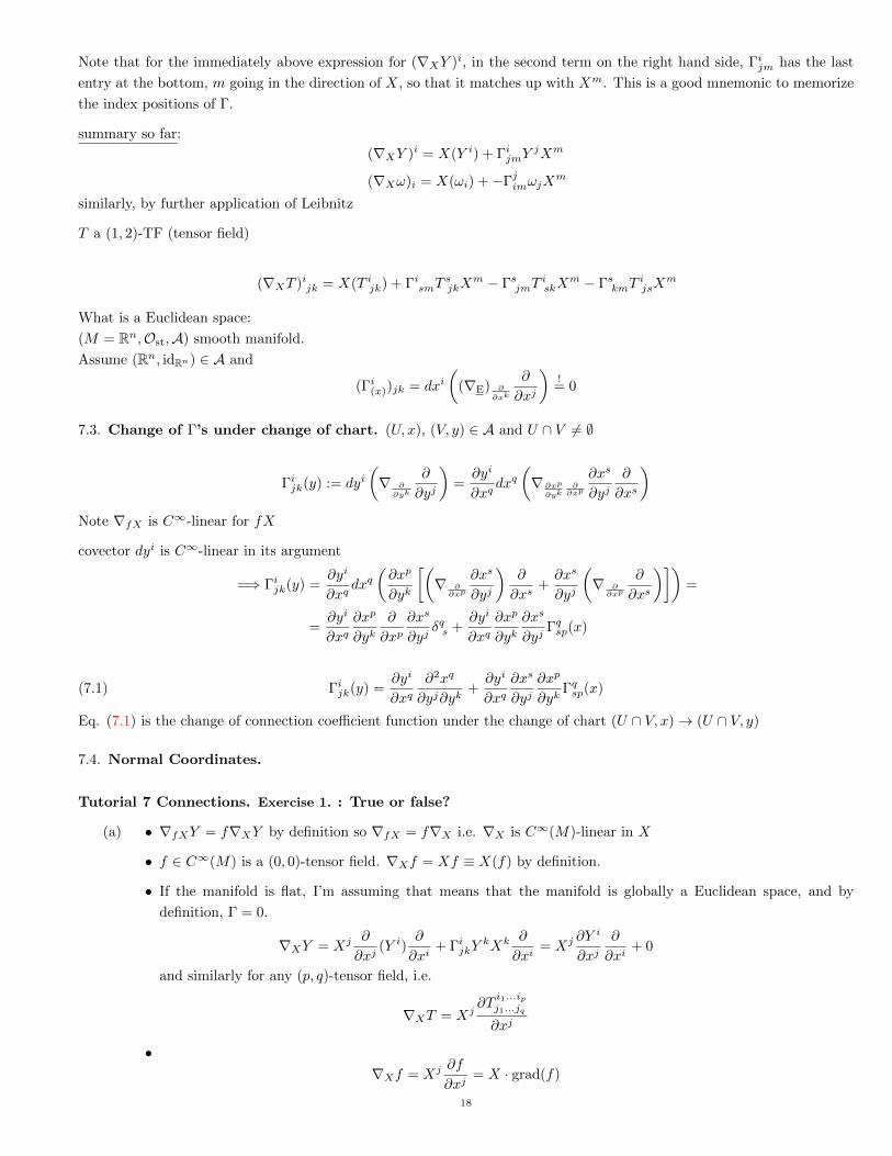
Note that for the immediately above expression for (∇XY )i, in the second term on the right hand side, Γijm has the last

entry at the bottom, m going in the direction of X, so that it matches up with Xm. This is a good mnemonic to memorize

the index positions of Γ.

summary so far:

(∇XY )i = X(Y i) + ΓijmYjXm

(∇Xω)i = X(ωi) +−ΓjimωjXm

similarly, by further application of Leibnitz

T a (1, 2)-TF (tensor field)

(∇XT )ijk = X(T ijk) + ΓismTsjkX

m − ΓsjmTiskX

m − ΓskmTijsX

m

What is a Euclidean space:

(M = Rn,Ost,A) smooth manifold.

Assume (Rn, idRn) ∈ A and

(Γi(x))jk = dxi(

(∇E) ∂

∂xk

∂

∂xj

)!= 0

7.3. Change of Γ’s under change of chart. (U, x), (V, y) ∈ A and U ∩ V 6= ∅

Γijk(y) := dyi(∇ ∂

∂yk

∂

∂yj

)=∂yi

∂xqdxq

(∇ ∂xp

∂yk∂∂xp

∂xs

∂yj∂

∂xs

)Note ∇fX is C∞-linear for fX

covector dyi is C∞-linear in its argument

=⇒ Γijk(y) =∂yi

∂xqdxq

(∂xp

∂yk

[(∇ ∂

∂xp

∂xs

∂yj

)∂

∂xs+∂xs

∂yj

(∇ ∂

∂xp

∂

∂xs

)])=

=∂yi

∂xq∂xp

∂yk∂

∂xp∂xs

∂yjδqs +

∂yi

∂xq∂xp

∂yk∂xs

∂yjΓqsp(x)

(7.1) Γijk(y) =∂yi

∂xq∂2xq

∂yj∂yk+∂yi

∂xq∂xs

∂yj∂xp

∂ykΓqsp(x)

Eq. (7.1) is the change of connection coefficient function under the change of chart (U ∩ V, x)→ (U ∩ V, y)

7.4. Normal Coordinates.

Tutorial 7 Connections. Exercise 1. : True or false?

(a) • ∇fXY = f∇XY by definition so ∇fX = f∇X i.e. ∇X is C∞(M)-linear in X

• f ∈ C∞(M) is a (0, 0)-tensor field. ∇Xf = Xf ≡ X(f) by definition.

• If the manifold is flat, I’m assuming that means that the manifold is globally a Euclidean space, and by

definition, Γ = 0.

∇XY = Xj ∂

∂xj(Y i)

∂

∂xi+ ΓijkY

kXk ∂

∂xi= Xj ∂Y

i

∂xj∂

∂xi+ 0

and similarly for any (p, q)-tensor field, i.e.

∇XT = Xj∂T

i1...ipj1...jq

∂xj

•∇Xf = Xj ∂f

∂xj= X · grad(f)

18

• ∀ (U, x) ∈ A, locally (after working out the first few cases, and doing induction, one can look up the expression

for the local form; I found it in Nakahara’s Geometry, Topology and Physics, Eq. 7.26, and it needs to

be modified for the convention of order of bottom indices for Γ:

∇νtλ1...λpµ1...µq = ∂νt

λ1...λpµ1...µq + Γλ1

κνtκλ2...λpµ1...µq + · · ·+ Γλpκνt

λ1...λp−1κµ1...µq − Γκµ1νt

λ1...λpκµ2...µq − · · · − Γκµqνt

λ1...λpµ1...µq−1κ

Clearly, ∇X is uniquely fixed ∀ p ∈M by choosing each of the (dimM)3 many connection coefficient functions

Γ.

(b) • ∇ : X(M)→ X(M)

∇ : (p, q)-tensor field 7→ (p, q)-tensor field

• By definition, ∇ satisfies the Leibniz rule.

•

•

•

Exercise 2. : Practical rules for how ∇ acts Torsion-free covariant derivative boils down to a connection coefficient

function Γ that is symmetric in the bottom indices.

•

∇Xf = X(f) = Xi ∂f

∂xi

•

(∇XY )a = Xi ∂Ya

∂xi+ ΓajkY

jXk

•

(∇Xω)a = Xi ∂ωa∂xj− ΓiakωiX

k

•

(∇mT )abc =∂

∂xm(T abc) + ΓaimT

ibc − ΓibmT

aic − ΓjcmT

abj

•

(∇[mA)n] = (∇mA)n − (∇nA)m =∂An∂xm

− ΓinmAi −(∂Am∂xn

− ΓimnAi

)=∂Am∂xm

− ∂Am∂xn

•

(∇mω)nr =∂ωnr∂xm

− Γinmωir − Γirmωni

Exercise 3. : Connection coefficients

Question .

The connection coefficient functions Γ in chart (U ∩ V, y) is given, in terms of chart (U ∩ V, x) as follows:

Recall Eq. (7.1)

Γijk(y) =∂yi

∂xq∂2xq

∂yj∂yk+∂yi

∂xq∂xs

∂yj∂xp

∂ykΓqsp(x)

19

8. Lecture 8: Parallel Transport & Curvature (International Winter School on Gravity and Light

2015)

8.1. Parallelity of vector fields.

Definition 15. (1) parallely transported along smooth curve γ : R→M

if

(8.1) ∇vγX = 0

(2) A slightly weaker condition

is “parallel”

(∇vγ,γ(λ)X)γ(λ) = µ(λ)Xγ(λ)

8.2. Autoparallely transported curves.

Definition 16. curve γ : R→M is called

autoparallely transported if

(8.2) ∇vγvγ!= 0

8.3. Autoparallel equation.

∇vγvγ = 0

in summary:

(8.3) γm(x)(λ) + (Γm(x))ab(γ(λ))γa(x)(λ)γb(x)(λ) = 0

8.4. Torsion.

Definition 17. torsion of a connection ∇ is the (1, 2)-tensor field

(8.4) T (ω,X, Y ) := ω(∇XY −∇YX − [X,Y ])

(Inside a cloud)

[X,Y ] vector field defined by

[X,Y ]f := X(Y f)− Y (Xf)

Proof. check T is C∞-linear in each entry

T (ω, fX, Y ) = ω(∇fXY −∇Y (fX)− [fX, Y ])

Definition 18. A (M,O,A,∇) is called torsion-free if T = 0

In a chart

T iab := T

(dxi,

∂

∂xa,∂

∂xb

)= dxi(. . . )

= Γiab − Γiba = 2Γi[ab]

From now on, in these lectures, we only use torsion-free connections.20

8.5. 4. Curvature.

Definition 19. Riemann curvature of a connection ∇ is the (1, 3)-tensor field

(8.5) Riem(ω,Z,X, Y ) := ω(∇X∇Y Z −∇Y∇XZ −∇[X,Y ]Z)

Proof. do it: C∞-linear in each slot.

Tutorials Riemijab = . . .

Tutorial 8 Parallel transport & Curvature

Exercise 1.

Exercise 2. : Where connection coefficients appear

It was suggested in the tutorial sheets and hinted in the lecture that the following should be committed to memory.

Question : Recall the autoparallel equation for a curve γ.

(a)

∇vγvγ = 0

(b)

∇vγvγ = ∇γ ∂∂xµ

vγ = γν∇∂νvγ = γν[∂vµγ∂xν

+ Γρµνvµγ

]∂

∂xρ= γν

[∂γρ

∂xν+ Γρµν γ

µ

]∂

∂xρ= 0

=⇒ γρ + Γρµν γµγν

as, for example, for F (x(t)),dF (x(t))

dt= x

∂F

∂x=

d

dtF

so that

γν∂vµγ∂xν

=d

dλvµγ =

d2

dλ2γµ

Question : Determine the coefficients of the Riemann tensor with respect to a chart (U, x).

Recall this manifestly covariant definition

Riem(ω,Z,X, Y ) = ω(∇X∇Y Z −∇Y∇XZ −∇[X,Y ]Z)

We want Rijab.

now

∇X∇Y Z = ∇X((Y µ∂

∂xµZρ + ΓρµνZ

µY ν)∂

∂xρ) = (Xα ∂

∂xα(Y µ

∂

∂xµZρ + ΓρµνZ

µY ν) + Γραβ(Y µ∂

∂xµZα + ΓαµνZ

µY ν)Xβ)∂

∂xρ

For X = ∂a, Y = ∂b, Z = ∂j , then the partial derivatives of the coefficients of the input vectors become zero.

=⇒ ∇∂a∇∂b∂j =∂

∂xa(Γijb) + ΓiαaΓαjb

Now

[X,Y ]i = Xj ∂

∂xjY i − Y j ∂X

i

∂xj

For coordinate vectors, [∂i, ∂j ] = 0 ∀ i, j = 0, 1 . . . d.

Thus

Rijab =∂

∂xaΓijb −

∂

∂xbΓija + ΓiαaΓαjb − ΓiαbΓ

αja

21

Question :Ric(X,Y ) := RiemmambX

aY b define (0, 2)-tensor?.

Yes, transforms as such:

EY developments. I roughly follow the spirit in Theodore Frankel’s The Geometry of Physics: An Introduction

Second Ed. 2003, Chapter 9 Covariant Differentiation and Curvature, Section 9.3b. The Covariant Differential of a Vector

Field. P.S. EY : 20150320 I would like a copy of the Third Edition but I don’t have the funds right now to purchase

the third edition: go to my tilt crowdfunding campaign, http://ernestyalumni.tilt.com, and help with your financial

support if you can or send me a message on my various channels and ernestyalumni gmail email address if you could help

me get a hold of a digital or hard copy as a pro bono gift from the publisher or author.

The spirit of the development is the following:

“How can we express connections and curvatures in terms of forms?” -Theodore Frankel.

From Lecture 7, connection ∇ on vector field Y , in the “direction” X,

∇ ∂

∂xkY =

(∂Y i

∂xk+ ΓijkY

j

)∂

∂xi

Make the ansatz (approche, impostazione) that the connection ∇ acts on Y , the vector field, first:

∇Y (X) =

(Xk ∂Y

i

∂xk+ ΓijkY

jXk

)∂

∂xi= Xk

(∇ ∂

∂xkY)i ∂

∂xi= (∇XY )i

∂

∂xi= ∇XY

Now from Lecture 7, Definition for Γ,

dxi(∇ ∂

∂xk

∂

∂xj

)= Γijk

Make this ansatz (approche, impostazine)

∇ ∂

∂xj=(Γijkdx

k)⊗ ∂

∂xi∈ Ω1(M,TM) = T ∗M ⊗ TM

where Ω1(M,TM) = T ∗M ⊗ TM is the set of all TM or vector-valued 1-forms on M , with the 1-form being the follow-

ing:

Γijkdxk = Γij ∈ Ω1(M) i = 1 . . . dim(M)

j = 1 . . . dim(M)

So Γij is a dimM × dimM matrix of 1-forms (EY !!!).

Thus

∇Y = (d(Y i) + ΓijYj)⊗ ∂

∂xi

So the connection is a (smooth) map from TM to the set of all vector-valued 1-forms on M , Ω1(M,TM), and then, after

“eating” a vector Y , yields the “covariant derivative”:

∇ : TM → Ω1(M,TM) = T ∗M ⊗ TM

∇ : Y 7→ ∇Y

∇Y : TM → TM

∇Y (X) 7→ ∇Y (X) = ∇X(Y )

Now [∂

∂xi,∂

∂xj

]f =

∂

∂xi

(∂

∂xj

)− ∂

∂xj

(∂

∂xi

)= 0

(this is okay as on p ∈ (U, x); x-coordinates on same chart (U, x))22

EY : 20150320 My question is when is this nontrivial or nonvanishing (i.e. not equal to 0).

[ea, eb] =?

for a frame (ec) and would this be the difference between a tangent bundle TM vs. a (general) vector bundle?

Wikipedia helps here. cf. wikipedia, “Connection (vector bundle)”

∇ : Γ(E)→ Γ(T ∗M ⊗ E) = Ω1(M,E)

∇ea = ωcabfb ⊗ ec

f b ∈ T ∗M (this is the dual basis for TM and, note, this is for the manifold, M

∇fbea = ωcabec ∈ E

ωca = ωcabfb ∈ Ω1(M)

is the connection 1-form, with a, c = 1 . . . dimV . EY : 20150320 This V is a vector space living on each of the fibers of E.

I know that Γ(T ∗M ⊗ E) looks like it should take values in E, but it’s meaning that it takes vector values of V . Correct

me if I’m wrong: ernestyalumni at gmail and various social media.

Let σ ∈ Γ(E), σ = σaea∇σ = (dσc + ωcabσ

af b)⊗ ec with

dσc =∂σc

∂xbf b

=⇒ ∇Xσ =

(Xb ∂σ

c

∂xb+ ωcabσ

aXb

)ec = Xb

(∂σc

∂xb+ ωcabσ

a

)ec

9. Lecture 9: Newtonian spacetime is curved!

Axiom 1 (Newton I:). A body on which no force acts moves uniformly along a straight line

Axiom 2 (Newton II:). Deviation of a body’s motion from such uniform straight motion is effected by a force, reduced by

a factor of the body’s reciprocal mass.

Remark:

(1) 1st axiom - in order to be relevant - must be read as a measurement prescription for the geometry of space . . .

(2) Since gravity universally acts on every particle, in a universe with at least two particles, gravity must not be

considered a force if Newton I is supposed to remain applicable.

9.1. Laplace’s questions. Laplace ∗ 1749

†1827

Q: “Can gravity be encoded in a curvature of space, such that its effects show if particles under the influence of (no other)

force we postulated to more along straight lines in this curved space?”

Answer: No!

Proof. gravity is a force point of view

mxα(t) = Fα(x(t))

mxα(t) = mfα︸︷︷︸Fα

(x(t))

−∂αfα = 4πGρ (Poisson)

ρ mass density of matter23

(EY : 20150330) You know this, F = Gm1m2/r2

xα(t)− fα(x(t)) = 0

Laplace asks: Is this (x(t)) of the form

xα(t) + Γαβγ(x(t))xβ(t)xγ(t) = 0

Conclusion: One cannot find Γ s such that Newton’s equation takes the form of an autoparallel.

9.2. The full wisdom of Newton I. use also the information from Newton’s first law that particles (no force) move

uniformly

introduce the appropriate setting to talk about the difference easily

insight: in spacetime uniform & straight motion is simply straight motion

So let’s try in spacetime:

let x : R→ R3

be a particle’s trajectory in space ←→ worldline (history) of the particleX : R→ R4

t 7→ (t, x1(t), x2(t), x3(t)) :=

:= (X0(t), X1(t), X2(t), X3(t))

That’s all it takes:

Trivial rewritings:

X0 = 1

=⇒X0 = 0

Xα − fα(X(t)) · X0 · X0 = 0(α = 1, 2, 3) =⇒

a = 0, 1, 2, 3

Xa + ΓabcXbXc = 0

antoparallel eqn in spacetime

Yes, choosing Γ0ab = 0

Γαβγ = 0 = Gammaα0β = Γαβ0

only: Γα00!= −fα

Question: Is this a coordinate-choice artifact?

No, since Rα0β0 = − ∂∂xβ

fα (only non-vanishing components) (tidal force tensor, − the Hessian of the force compo-

nent)

Ricci tensor =⇒ R00 = Rm0m0 = −∂αfα = 4πGρ

Poisson: −∂αfα = 4πG · ρ

writing: T00 = 12s

=⇒ R00 = 8πGT00

Einstein in 1912 (((((((hhhhhhhRab = 8πGTab

24

Conclusion: Laplace’s idea works in spacetime

Remark

Γα00 = −fα

Rαβγδ = 0 α, β, γ, δ = 1, 2, 3

R00 = 4πGρ

Q: What about transformation behavior of LHS of

xa + ΓabcXbXc︸ ︷︷ ︸

(∇vXvX)a︸ ︷︷ ︸:=aa “acceleration vector”

= 0

9.3. The foundations of the geometric formulation of Newton’s axiom. new start

Definition 20. A Newtonian spacetime is a quintuple

(M,O,A,∇, t)

where (M,O,A) 4-dim. smooth manifold

t : M → R smooth function

(i) “There is an absolute space”

(dt)p 6= 0 ∀ p ∈M

(ii) “absolute time flows uniformly”

∇dt =︸︷︷︸space of (0, 2)-tensor fields

0 everywhere

∇dt is a (0, 2)-tensor field

(iii) add to axioms of Newtonian spacetime ∇ = 0 torsion free

Definition 21. absolute space at time τ

Sτ := p ∈M |t(p) = τdt6=0−−−→M =

∐Sτ

Definition 22. A vector X ∈ TpM is called

(a) future-directed if

dt(X) > 0

(b) spatial if

dt(X) = 0

(c) past-directed if

dt(X) < 0

picture

Newton I: The worldline of a particle under the influence of no force (gravity isn’t one, anyway) is a future-directed autoparallel

i.e.

∇vXvX = 0

dt(vX) > 0

25

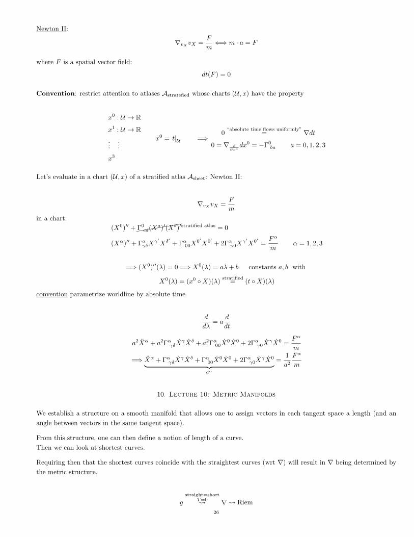
Newton II:

∇vXvX =F

m⇐⇒ m · a = F

where F is a spatial vector field:

dt(F ) = 0

Convention: restrict attention to atlases Astratefied whose charts (U , x) have the property

x0 : U → R

x1 : U → R...

...

x3

x0 = t|U =⇒0

“absolute time flows uniformly”= ∇dt

0 = ∇ ∂∂xa

dx0 = −Γ0ba a = 0, 1, 2, 3

Let’s evaluate in a chart (U , x) of a stratified atlas Asheet: Newton II:

∇vXvX =F

m

in a chart.

(X0)′′ +(((((((Γ0

cd(Xa)′(Xb)′stratified atlas = 0

(Xα)′′ + ΓαγδXγ′Xδ′ + Γα00X

0′X0′ + 2Γαγ0Xγ′X0′ =

Fα

mα = 1, 2, 3

=⇒ (X0)′′(λ) = 0 =⇒ X0(λ) = aλ+ b constants a, b with

X0(λ) = (x0 X)(λ)stratified

= (t X)(λ)

convention parametrize worldline by absolute time

d

dλ= a

d

dt

a2Xα + a2ΓαγδXγXδ + a2Γα00X

0X0 + 2Γαγ0XγX0 =

Fα

m

=⇒ Xα + ΓαγδXγXδ + Γα00X

0X0 + 2Γαγ0XγX0︸ ︷︷ ︸

aα

=1

a2

Fα

m

10. Lecture 10: Metric Manifolds

We establish a structure on a smooth manifold that allows one to assign vectors in each tangent space a length (and an

angle between vectors in the same tangent space).

From this structure, one can then define a notion of length of a curve.

Then we can look at shortest curves.

Requiring then that the shortest curves coincide with the straightest curves (wrt ∇) will result in ∇ being determined by

the metric structure.

gstraight=short

T=0 ∇ Riem

26

10.1. Metrics.

Definition 23. A metric g on a smooth manifold (M,O,A) is a (0, 2)-tensor field satisfying

(i) symmetry g(X,Y ) = g(Y,X) ∀X,Y vector fields

(ii) non-degeneracy: the musical map

“flat” [ : Γ(TM)→ Γ(T ∗M)

X 7→ [(X)

where [(X)(Y ) := g(X,Y )

[(X) ∈ Γ(T ∗M)

In thought bubble: [(X) = g(X, ·)

. . . is a C∞-isomorphism in other words, it is invertible.

Remark: ([(X))a or

Xa

([(X))a := gamXm

Thought bubble: [−1 = ]

[−1(ω)a := gamωm

[−1(ω)a := (g“−1′′)amωm =⇒ not needed. (all of this is not needed)

Definition 24. The (2, 0)-tensor field g“−1′′ with respect to a metric g is the symmetric

g“−1′′ : Γ(T ∗M)× Γ(T ∗M) −→ C∞(M)

(ω, σ) 7→ ω([−1(σ)) [−1(σ) ∈ Γ(TM))

chart: gab = gba

(g−1)amgmb = δab

Example: (S2,O,A)

chart (U , x)

ϕ ∈ (0, 2π)

θ ∈ (0, π)

define the metric

gij(x−1(θ, ϕ)) =

[R2 0

0 R2 sin2 θ

]ij

R ∈ R+

“the metric of the round sphere of radius R”27

10.2. Signature. Linear algebra:

Aamvm = λva

λ1 0

. . .

0 λn

gamvm = λ · va?

1. . .

1

−1. . .

−1

0. . .

0

(1, 1) tensor has eigenvalues

(0, 2) has signature (p, q) (well-defined)

(+ + +)

(+ +−)

(+−−)

(−−−)

d+ 1 if p+ q = dimV

Definition 25. A metric is called

Riemannian if its signature is (+ + · · ·+)

Lorentzian if (+− · · ·−)

10.3. Length of a curve. Let γ be a smooth curve.

Then we know its veloctiy vγ,γ(λ) at each γ(λ) ∈M .

Definition 26. On a Riemannian metric manifold M,O,A, g), the speed of a curve at γ(λ) is the number

(√g(vγ , vγ))γ(λ) = s(λ)

F. Schuller: “I feel the need for speed.” -Top Gun.

(I feel the need for speed, then I feel the need for a metric)

Aside: [va] = 1T

[gab] = L2

[√gabvavb] =

√L2

T 2 = LT

Definition 27. Let γ : (0, 1)→M a smooth curve.

Then the length of γ is the number

R 3 L[γ] :=

∫ 1

0

dλs(λ) =

∫ 1

0

dλ√

(g(vγ , vγ))γ(λ)

F. Schuller: “velocity is more fundamental than speed, speed is more fundamental than length”

Example: reconsider the round sphere of radius R

Consider its equator:

θ(λ) := (x1 γ)(λ) =π

2

ϕ(λ) := (x2 γ)(λ) = 2πλ3

28

θ′(λ) = 0

ϕ′(λ) = 6πλ2

on the same chart gij =

[R2

R2 sin2 θ

]F.Schuller: do everything in this chart

L[γ] =

∫ 1

0

dλ√gij(x−1(θ(λ), ϕ(λ)))(xi γ)′(λ)(xj γ)′(λ) =

∫ 1

0

dλ

√R2 · 0 +R2 sin2 (θ(λ))36π2λ4 =

= 6πR

∫ 1

0

dλλ2 = 6πR[1

3λ3]10 = 2πR

Theorem 4. γ : (0, 1)→M and

σ : (0, 1)→ (0, 1) smooth bijective and increasing “reparametrization”

L[γ] = L[γ σ]

Proof. =⇒ Tutorials

10.4. Geodesics.

Definition 28. A curve γ : (0, 1) → M is called a geodesic on a Riemannian manifold (M,O,A, g) if its a stationary

curve with respect to a length functional L.

Thought bubble: in classical mechanics, deform the curve a little, ε times this deformation, to first order, it agrees with

L[γ]

Theorem 5. γ geodesic iff it satisfies the Euler-Lagrange equations for the Lagrangian

L :TM → R

X 7→√g(X,X)

In a chart, the Euler Lagrange equations take the form:(∂L∂xm

)·− ∂L∂xm

= 0

F.Schuller: this is a chart dependent formulation

here:

L(γi, γi) =√gij(γ(λ))γi(λ)γj(λ)

Euler-Lagrange equations:

∂L∂γm

=1√. . .gmj(γ(λ))γj(λ)

(∂L∂γm

)·=

(1√. . .

)·gmj(γ(λ)) · γj(λ) +

1√. . .

(gmj(γ(λ))γj(λ) + γs(∂sgmj)γ

j(λ))

Thought bubble: reparametrize g(γ, γ) = 1 (it’s a condition on my reparametrization)

By a clever choice of reparametrization ( 1√... )· = 0

∂L∂γm

=1

2√. . .∂mgij(γ(λ))γi(λ)γj(λ)

putting this together as Euler-Lagrange equations:

gmj γj + ∂sgmj γ

sγj − 1

2∂mgij γ

iγj = 0

29

Multiply on both sides (g−1)qm

γq + (g−1)qm(∂igmj −1

2∂mgij)γ

iγj = 0

γq + (g−1)qm1

2(∂igmj + ∂jgmi − ∂mgij)γiγj = 0

geodesic equation for γ in a chart.

(g−1)qm1

2(∂igmj + ∂jgmi − ∂mgij) =: Γqij(γ(λ))

Thought bubble:(

∂L∂ξa+dimMx

)·σ(x)−(∂L∂xiax

)σ(x)

= 0

Definition 29. “Christoffel symbol” L.C.Γ are the connection coefficient functions of the so-called Levi-Civita connectionL.C.∇

We usually make this choice of ∇ if g is given.

(M,O,A, g)→ (M,O,A, g, L.C.∇)

abstract way: ∇g = 0 and T = 0 (torsion)

=⇒ ∇ = L.C.∇

Definition 30. (a) The Riemann-Christoffel curvature is defined by

Rabcd := gamRmbcd

(b) Ricci: Rab = RmambThought bubble: with a metric, L.C.∇

(c) (Ricci) scalar curvature:

R = gabRab

Thought bubble: L.C.∇

Definition 31. Einstein curvature (M,O,A, g)

Gab := Rab −1

2gabR

Convention: gab := (g“−1′′)ab

F. Schuller: these indices are not being pulled up, because what would you pull them up with

(student) Question: Does the Einstein curvature yield new information?

Answer:

gabGab = Rabgab − 1

2gabg

abR = R− δaaR = R− 1

2dimM R = (1− d

2)R

Tutorial 9: Metric manifolds. Exercise 3: Levi-Civita Connection. Suppose torsion-free T = 0 and metric-

compatible connection ∇g = 0

Question Recall T = 0 on a chart.

Γcba =1

2(g−1)cm

(∂gbm∂xa

+∂gma∂xb

− ∂gab∂xm

)or

Γabc =1

2(g−1)am

(∂gbm∂xc

+∂gmc∂xb

− ∂gbc∂xm

)30

11. Symmetry

EY : 20150321 This lecture tremendously and lucidly clarified, for me at least, what a symmetry of the Lie algebra is, and

in comparing structures (M,O,A) vs. (M,O,A,∇), clarified differences, and asking about differences is a good way to

learn, the difference between L and ∇, respectively.

Feeling that the round sphere

(S2,O,A, ground)

has rotational symmetry, while

the potato

(S2,O,A, gpotato)

does not.

11.1.

11.2. Important

11.3. Flow of a complete vector field. Let (M,O,A) smooth X vector field on M

Definition 32. A curve γ : I ⊆ R→M is called an integral curve of X

if

vγ,γ(λ) = Xγ(λ)

Definition 33. A vector filed X is complete if all integral curves have I = R EY: 20150321 (i.e. domain is all of R)

Ex. minute 48:30 EY : reall good explanation by F.P.Schuller; take a pt. out for an incomplete vector field.

Theorem 6. compactly supported smooth vector field is complete.

Definition 34. The flow of a complete vector field X is a 1-parameter family

hX = R×M →M

where γp : R→M

γ(0) = p

is the integral curve of X with

Then for fixed λ ∈ RhXλ : M →M smooth

picture hXλ (S) 6= S( if X 6= 0)

11.4. Lie subalgebras of the Lie algebra (Γ(TM), [·, ·]) of vector fields.

(a) Γ(TM) = set of all vector fields C∞(M)-module = R-vector space

=⇒ [X,Y ] ∈ Γ(TM) [X,Y ]f := X(Y f)− Y (Xf)

(i) [X,Y ] = −[Y,X]

(ii) [λX + Z, Y ] = λ[X,Y ] + [Z, Y ]

(iii) [X, [Y,Z]] + [Z, [X,Y ]] + [Y, [Z,X]] = 0

(Γ(TM), [·, ·]) Lie algebra

(b) Let X1 . . . Xs for s (many) vector fields on M , such that

31

Tutorial 11 Symmetry. Exercise 1. : True or false?

(a) •

• φ∗ : T ∗N → T ∗M i.e. φ∗ν(X) = ν(φ∗X) for smooth φ : M → N , so the pullback of a covector ν ∈ T ∗Nmaps to a covector in T ∗M .

•

•

•

•

(b)

(c)

Exercise 2. : Pull-back and push-forward

Question . Let’s check this locally

φ∗(df)(X) = (df)(φ∗X) = (df)(Xi ∂yj

∂xi∂

∂yj) = Xi ∂y

j

∂xi∂f

∂yjwhere φ∗X = Xi ∂y

j

∂xi∂

∂yj

d(φ∗f)(X) = d(f(φ))(X) =∂f

∂yj∂yj

∂xidxi(X) = Xi ∂y

j

∂xi∂f

∂yj

So

φ∗(df) = d(φ∗f) ∀ p ∈M, ∀X ∈ X(M)

The big idea is that this is a showing of the naturality of the pullback φ∗ with d, i.e. that this commutes:

Ω1(M) Ω1(N)

C∞(M) C∞(N)

φ∗

d

φ∗

d

Question .

(φ∗)ab := (dya)(φ∗(

∂

∂xb))

Let g ∈ C∞(N)

φ∗

(∂

∂xb

)g =

∂xb

gφ(p) =

∂

∂xbgφx−1x(p) =

∂

∂xb(gyy−1φx−1)(x) =

=∂

∂xb(gy−1(yφx−1(x(p)))) =

∂g

∂y

b∣∣∣∣∣y

∂ya

∂xb

∣∣∣∣x

=∂ya

∂xb∂g

∂ya

Then

φ∗

(∂

∂xb

)=∂ya

∂xb∂

∂ya

and so

(φ∗)ab =

∂ya

∂xb

Question .

Exercise 3. :Lie derivative-the pedestrian way

Question . While it is true that ∀ p ∈ S2, for x(p) = (θ, ϕ), and (yix−1)(θ, ϕ) = (y1, y2, y3) ∈ R3 and that, at this point

p, (y1)2/a2 + (y2)2/b2 + (y3)2/c3 = 1, this doesn’t imply (EY: 20150321 I think) that, globally, it’s an ellipsoid (yet). In

the familiar charts given,32

spherical chart (U, x) ∈ A and

(R3, y = idR3) ∈ Bit looks like an ellipsoid, but change to another choice of charts, and it could look something very different.

Question .

Equip (R3,Ost,B) with the Euclidean metric g, and pullback g.

Note that the pullback of the inclusion from R3 onto S2 for the Euclidean metric is the following:

i∗g

(∂

∂θi,∂

∂θj

)= g

(i∗

∂

∂θi, i∗

∂

∂θj

)= g

(∂xa

∂θi∂

∂xa,∂xb

∂θj∂

∂xb

)= gab

∂xa

∂θi∂xb

∂θj

With gab = δab, the usual Euclidean metric, this becomes the following:

gellipsoidij =

∂xa

∂θi∂xa

∂θj

At this point, one should get smart (we are in the 21st century) and use some sort of CAS (Computer Algebra System). I

like Sage Math (version 6.4 as of 20150322). I also like the Sage Manifolds package for Sage Math.

I like Sage Math for the following reasons:

• Open source, so its open and freely available to anyone, which fits into my principle of making online education

open and freely available to anyone, anytime

• Sage Math structures everything in terms of Category Theory and Categories and Morphisms naturally correspond

to Classes and Class methods or functions in Object-Oriented Programming in Python and theyve written it that

way

and I like Sage Manifolds for roughly the same reasons, as manifolds are fit into a category theory framework thats written

into the Python code. e.g.

sage: S2 = Manifold(2, ’S^2’, r’\mathbbS^2’, start_index=1) ; print S2

sage: print S2

2-dimensional manifold ’S^2’

sage: type(S2)

<class ’sage.geometry.manifolds.manifold.Manifold_with_category’>

With code (Ive provided for convenience; you can make your own as I wrote it based upon to example of S2 on the

sagemanifolds documentation website page), load it and do the following:

cf. https://github.com/ernestyalumni/diffgeo-by-sagemnfd/blob/master/S2.sage

http://sagemanifolds.obspm.fr/examples.html

sage: load("S2.sage")

sage: U_ep = S2.open_subset(’U_ep’)

sage: eps.<the,phi> = U_ep.chart()

sage: a = var(a)

sage: b = var(b)

sage: c = var("c")

sage: inclus = S2.diff_mapping(R3, (eps, cart): [ a*cos(phi)*sin(the), b*sin(phi)*sin(the),c*cos(the) ] , name="inc",latex_name=r’\mathcali’)

sage: inclus.pullback(h).display()

inc_*(h) = (c^2*sin(the)^2 + (a^2*cos(phi)^2 + b^2*sin(phi)^2)*cos(the)^2) dthe*dthe - (a^2 - b^2)*cos(phi)*cos(the)*sin(phi)*sin(the) dthe*dphi

- (a^2 - b^2)*cos(phi)*cos(the)*sin(phi)*sin(the) dphi*dthe + (b^2*cos(phi)^2 + a^2*sin(phi)^2)*sin(the)^2 dphi*dphi

sage: inclus.pullback(h)[2,2].expr()

(b^2*cos(phi)^2 + a^2*sin(phi)^2)*sin(the)^2

A new open subset Uep was declared in S2, a new chart (Uep, (θ, φ)) was declared, the constants, a, b, c, were declared, and

the inclusion map given in the problem

y i x−1 : (θ, φ) 7→ (a cosφ sin θ, b sinφ sin θ, c cos θ)

Then the pullback of the inclusion map 〉 was done on the Euclidean metric h, defined earlier in the file

S2.sage

33

. Then one can access the components of this metric and do, for example,

simplify_full(),full_simplify(), reduce_trig()

on the expression.

In Python, I could easily do this, and give an answer quick in LaTeX:

sage: for i in range(1,3):

....: for j in range(1,3):

....: print inclus.pullback(h)[i,j].expr()

....: latex(inclus.pullback(h)[i,j].expr() )

....:

c^2*sin(the)^2 + (a^2*cos(phi)^2 + b^2*sin(phi)^2)*cos(the)^2

(EY: I’ll suppress the LaTeX output but this sage math function gives you LaTeX code)

and so

i∗g = c2 sin (the)2

+(a2 cos (φ)

2+ b2 sin (φ)

2)

cos (the)2dθ ⊗ dθ+

−2(a2 − b2

)cos (φ) cos (the) sin (φ) sin (the) dθ ⊗ dφ+

+(b2 cos (φ)

2+ a2 sin (φ)

2)

sin (the)2dφ⊗ dφ

Question .

sage: polar_vees = eps.frame()

sage: X_1 = - sin(phi) * polar_vees[1] - cot( the ) * cos(phi) * polar_vees[2]

sage: X_2 = cos( phi ) * polar_vees[1] - cot( the ) * sin( phi) * polar_vees[2]

sage: X_3 = polar_vees[2]

sage: X_2.lie_der(X_1).display()

(cos(the)^2 - 1)/sin(the)^2 d/dphi

sage: X_3.lie_der(X_1).display()

cos(phi) d/dthe - cos(the)*sin(phi)/sin(the) d/dphi

sage: X_3.lie_der(X_2).display()

sin(phi) d/dthe + cos(phi)*cos(the)/sin(the) d/dphi

Indeed, one can check on a scalar field feps ∈ C∞(S2):

sage: f_eps = S2.scalar_field(eps: function(’f’, the, phi ) , name=’f’ )

sage: (X_1( X_2(f_eps)) - X_2(X_1(f_eps) ) ).display()

U_ep --> R

(the, phi) |--> -D[1](f)(the, phi)

sage: X_2.lie_der(X_1) == -X_3

True

sage: X_3.lie_der(X_1) == X_2

True

sage: X_3.lie_der(X_2) == -X_1

True

=⇒ [Xi, Xj ] = −εijkXk

So spanRX1, X2, X3 equipped with [ , ] constitute a Lie subalgebra on S2 (It’s closed under [ , ]

12. Integration

12.1.34

12.2.

12.3. Volume forms.

Definition 35. On a smooth manifold (M,O,A)

a (0,dimM)-tensor field Ω is called a volume form if

(a) Ω vanishes nowhere (i.e. Ω 6= 0 ∀ p ∈M)

(b) totally antisymmetric

Ω(. . . , X︸︷︷︸ith

, . . . , Y︸︷︷︸jth

. . . ) = −Ω(. . . , Y︸︷︷︸ith

, . . . , X︸︷︷︸jth

. . . )

In a chart:

Ωi1...id = Ω[i1...id]

Example (M,O,A, g) metric manifold

construct volume form Ω from g

In any chart: (U, x)

Ωi1...id :=√

det(gij(x))εi1...id

where Levi-Civita symbol εi1...id is defined as ε123...d = +1

ε1...d = ε[i1...id]

Proof. (well-defined) Check: What happens under a change of charts

Ω(y)i1...id =√

det(g(y)ij)εi1...id =

=

√det(gmn(x)

∂xm

∂yi∂xn

∂yj)∂ym1

∂xi1. . .

∂ymd

∂xidε[m1...md] =

=√|detgij(x)|

∣∣∣∣det

(∂x

∂y

)∣∣∣∣det

(∂y

∂x

)εi1...id =

√detgij(x)εi1...idsgn

(det

(∂x

∂y

))

EY : 20150323

Consider the following:

Ω(y)(Y(1) . . . Y(d)) = Ω(y)i1...idYi1(1) . . . Y

id(d) =

=√

det(gij(y))εi1...idYi1(1) . . . Y

id(d) =

=

√det(gmn(x))

∂xm

∂yi∂xn

∂yjεi1...id

∂yi1

∂xm1. . .

∂yid

∂xmdXm1 . . . Xmd =

=

√det(gmn(x))

∂xm

∂yi∂xn

∂yjdet

(∂y

∂x

)εm1...mdX

m1 . . . Xmd =

=√

det(gmn(x))

∣∣∣∣det

(∂x

∂y

)∣∣∣∣det

(∂y

∂x

)εm1...mdX

m1 . . . Xmd =

=√

det(gmn(x))εm1...mdsgn

(det

(∂x

∂y

))Xm1 . . . Xmd = sgn(det

(∂x

∂y

))Ωm1...md(x)Xm1 . . . Xmd

35

If det(∂y∂x

)> 0,

Ω(y)(Y(1) . . . Y(d)) = Ω(x)(X(1) . . . X(d))

This works also if Levi-Civita symbol εi1...id doesn’t change at all under a change of charts. (around 42:43 https://youtu.

be/2XpnbvPy-Zg)

Alright, let’s require,

restrict the smooth atlas Ato a subatlas (A↑ still an atlas)

A↑ ⊆ A

s.t. ∀ (U, x), (V, y) have chart transition maps y x−1

x y−1

s.t. det(∂y∂x

)> 0

such A↑ called an oriented atlas

(M,O,A, g) =⇒ (M,O,A↑, g)

Note: associated bundles.

Note also: det(∂yb

∂xa

)= det(∂a(ybx−1)) ∂yb

∂xa is an endomorphism on vector space V . ϕ : V → V

detϕ independent of choice of basis

g is a (0, 2) tensor field, not endomorphism (not independent of choice of basis)√|det(gij(y))|

Definition 36. Ω be a volume form on (M,O,A↑) and consider chart (U, x)

Definition 37. ω(X) := Ωi1...idεi1...id same way ε12...d = +1

ε[... ]

one can show

ω(y) = det

(∂x

∂y

)ω(x) scalar density

12.4. Integration on one chart domain U .

Definition 38.

(12.1)

∫U

f :(U,y)=

∫y(U)

ddβω(y)(y−1(β))f(y)(β)

Proof. : Check that it’s (well-defined), how it changes under change of charts∫U

f :(U,y)=

∫y(U)

ddβω(y)(y−1(β))f(y)(β) = =

(U,y)

∫x(U)

∫ddα

∣∣∣∣det

(∂y

∂x

)∣∣∣∣ f(x)(α)ω(x)(x−1(α)det

(∂x

∂y

)=

=

∫x(U)

ddαω(x)(x−1(x))f(x)(α)

36

On an oriented metric manifold (M,O,A↑, g)∫U

f :=

∫x(U)

ddα√

det(gij(x))(x−1(α))︸ ︷︷ ︸√g

f(x)(α)

12.5. Integration on the entire manifold.

13. Lecture 13: Relativistic spacetime

Recall, from Lecture 9, the definition of Newtonian spacetime

(M,O,A,∇, t)

∇ torsion free

t ∈ C∞(M)

dt 6= 0

∇dt = 0 (uniform time)

and the definition of relativistic spacetime (before Lecture )

(M,O,A↑,∇, g, T )

∇ torsion-free

g Lorentzian metric(+−−−)

T time-orientation

13.1. Time orientation.

Definition 39. (M,O,A↑, g) a Lorentzian manifold. Then a time-orientation is given by a vector field T that

(i) does not vanish anywhere

(ii) g(T, T ) > 0

Newtonian vs. relativistic

Newtonian

X was called future-directed if

dt(X) > 0

∀ p ∈M , take half plane, half space of TpM

also stratified atlas so make planes of constant t straight

relativistic

half cone ∀ p, q ∈M , half-cone ⊆ TpM

This definition of spacetime

Question

I see how the cone structure arises from the new metric. I don’t understand however, how the T , the time orientation,

comes in

Answer

(M,O,A, g) g(←− +−−−)

requiring g(X,X) > 0, select cones

T chooses which cone

This definition of spacetime has been made to enable the following physical postulates:37

(P1) The worldline γ of a massive particle satisfies

(i) gγ(λ)(vγ,γ(lambda), vγ,γ(λ)) > 0

(ii) gγ(λ)(T, vγ,γ(λ)) > 0

(P2) Worldlines of massless particles satisfy

(i) gγ(λ)(vγ,γ(λ), vγ,γ(λ)) = 0

(ii) gγ(λ)(T, vγ,γ(λ)) > 0

picture: spacetime:

Answer (to a question) T is a smooth vector field, T determines future vs. past, “general relativity: we have such a time

orientation; smoothness makes it less arbitrary than it seems” -FSchuller,

Claim: 9/10 of a metric are determined by the cone

spacetime determined by distribution, only one-tenth error

13.2. Observers. (M,O,A↑,∇, g, T )

Definition 40. An observer is a worldline γ with

g(vγ , vγ) > 0

g(T, vγ) > 0

together with a choice of basis

vγ,γ(λ) ≡ e0(λ), e1(λ), e2(λ), e3(λ)

of each Tγ(λ)M where the observer worldline passes, if g(ea(λ), eb(λ)) = ηab =

1

−1

−1

−1

ab

precise: observer = smooth curve in the frame bundle LM over M

13.2.1. Two physical postulates.

(P3) A clock carried by a specific observer (γ, e) will measure a time

τ :=

∫ λ1

λ0

dλ√gγ(λ)(vγ,γ(λ), vγ,γ(λ))

between the two “events”

γ(λ0) “start the clock”

and

γ(λ1) “stop the clock”

Compare with Newtonian spacetime:

t(p) = 7

Thought bubble: proper time/eigentime τ

Application/Example.

M = R4

O = Ost

A 3 (R4, idR4)

g : g(x)ij = ηij ; T i(x) = (1, 0, 0, 0)i

=⇒ Γi(x) jk = 0 everywhere38

=⇒ (M,O,A↑, g, T,∇) Riemm = 0

=⇒ spacetime is flat

This situation is called special relativity.

Consider two observers:γ : (0, 1)→M

γi(x) = (λ, 0, 0, 0)i

δ : (0, 1)→M

α ∈ (0, 1) :δi(x) =

(λ, αλ, 0, 0)i λ ≤ 12

(λ, (1− λ)α, 0, 0)i λ > 12

let’s calculate:

τγ :=

∫ 1

0

√g(x)ij γ

i(x)γ

j(x) =

∫ 1

0

dλ1 = 1

τδ :=

∫ 1/2

0

dλ√

1− α2 +

∫ 1

1/2

√12 − (−α)2 =

∫ 1

0

√1− α2 =

√1− α2

Note: piecewise integration

Taking the clock postulate (P3) seriously, one better come up with a realistic clock design that supports the

postulate. idea.

2 little mirrors

(P4) Postulate

Let (γ, e) be an observer, and

δ be a massive particle worldline that is parametrized s.t. g(vγ , vγ) = 1 (for parametrization/normalization

convenience)

Suppose the observer and the particle meet somewhere (in spacetime)

δ(τ2) = p = γ(τ1)

This observer measures the 3-velocity (spatial velocity) of this particle as

(13.1) vδ : εα(vδ,δ(τ2))eα α = 1, 2, 3

where ε0, ε1, ε2, ε3 is the unique dual basis of e0, e1, e2, e3

EY:20150407

There might be a major correction to Eq. (13.1) from the Tutorial 14 : Relativistic spacetime, matter, and Gravitation,

see the second exercise, Exercise 2, third question:

(13.2) v :=εα(vδ)

ε0(vδ)eα

Consequence: An observer (γ, e) will extract quantities measurable in his laboratory from objective spacetime quantities

always like that.

Ex: F Faraday (0, 2)-tensor of electromagnetism:

F (ea, eb) = Fab =

0 E1 E2 E3

−E1 0 B3 −B2

−E2 −B3 0 B1

−E3 B2 −B1 0

observer frame ea, eb

39

Eα := F (e0, eα)

Bγ := F (eα, eρ)εαβγ where ε123 = +1 totally antisymmetric

13.3. Role of the Lorentz transformations. Lorentz transformations emerge as follows:

Let (γ, e) and (γ, e) be observers with γ(τ1) = γ(τ2)

(for simplicity γ(0) = γ(0)

Now

e0, . . . , e1 at τ = 0

and e0, . . . , e1 at τ = 0

both bases for the same Tγ(0)M

Thus: ea = Λbaeb Λ ∈ GL(4)

Now:

ηab = g(ea, eb) = g(Λmaem,Λnben) =

= ΛmaΛnb g(em, en)︸ ︷︷ ︸ηmn

i.e. Λ ∈ O(1, 3)

Result: Lorentz transformations relate the frames of any two observers at the same point.

“xµ − Λµνxν” is utter nonsense

Tutorial. I didn’t see a tutorial video for this lecture, but I saw that the Tutorial sheet number 14 had the relevant topics.

Go there.

14. Lecture 14: Matter

two types of matter

point matter

field matter

point matter

massive point particle

more of a phenomenological importance

field matter

electromagnetic field

more fundamental from the GR point of view

both classical matter types40

14.1. Point matter. Our postulates (P1) and (P2) already constrain the possible particle worldlines.

But what is their precise law of motion, possibly in the presence of “forces”,

(a) without external forces

Smassive[γ] := m

∫dλ√gγ(λ)(vγ,γ(λ), vγ,γ(λ))

with:

gγ(λ)(Tγ(λ), vγ,γ(λ)) > 0

dynamical law Euler-Lagrange equation

similarly

Smassless[γ, µ] =

∫dλµg(vγ,γ(λ), vγ,γ(λ))

δµ g(vγ,γ(λ), vγ,γ(λ)) = 0

δγ e.o.m.

Reason for describing equations of motion by actions is that composite systems have an action that is the sum of

the actions of the parts of that system, possibly including “interaction terms.”

Example.

S[γ] + S[δ] + Sint[γ, δ]

(b) presence of external forces

or rather presence of fields to which a particle “couples”

Example

S[γ;A] =

∫dλm

√gγ(λ)(vγ,γ(λ), vγ,γ(λ)) + qA(vγ,γ(λ))

where A is a covector field on M . A fixed (e.g. the electromagnetic potential)

Consider Euler-Lagrange eqns. Lint = qA(x)γm(x)

m(∇vγvγ)a +

˙(∂Lint

∂ ˙m(x)

)γ − ∂Lint

∂γm(x)︸ ︷︷ ︸∗

= 0 =⇒ m(∇vγvγ)a = −qF amγm︸ ︷︷ ︸Lorentz force on a charged particle in an electromagnetic field

∂L

∂γa= qA(x)a,

˙(∂L

∂ ˙m

)γ = q · ∂

∂xm(A(x)m) · γm(x)

∂L

∂γa= q · ∂

∂xa(A(x)m)γm

∗ = q

(∂Aa∂xm

− ∂Am∂xa

)γm(x) = q · F(x)amγ

m(x)

F ← Faraday

S[γ] =

∫(m√g(vγ , vγ) + qA(vγ))dλ

41

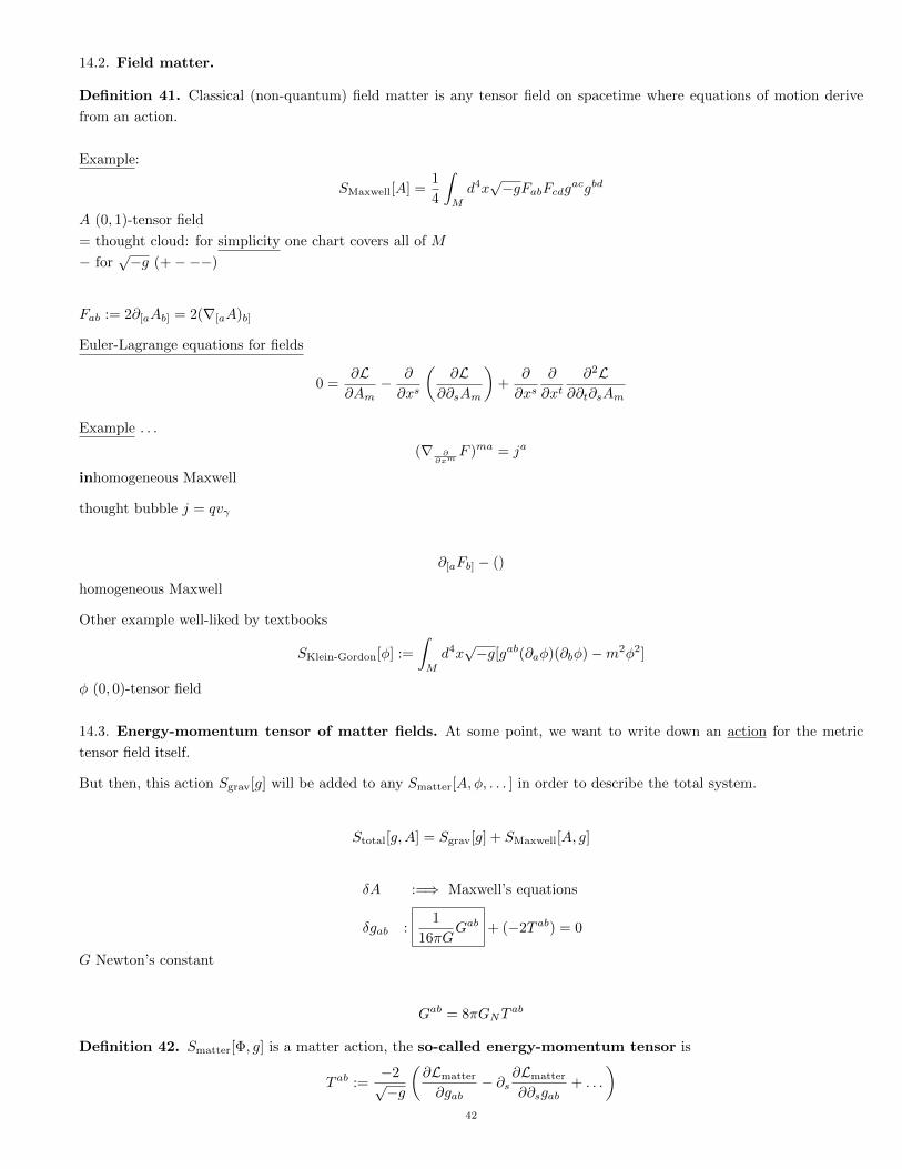
14.2. Field matter.

Definition 41. Classical (non-quantum) field matter is any tensor field on spacetime where equations of motion derive

from an action.

Example:

SMaxwell[A] =1

4

∫M

d4x√−gFabFcdgacgbd

A (0, 1)-tensor field

= thought cloud: for simplicity one chart covers all of M

− for√−g (+−−−)

Fab := 2∂[aAb] = 2(∇[aA)b]

Euler-Lagrange equations for fields

0 =∂L∂Am

− ∂

∂xs

(∂L

∂∂sAm

)+

∂

∂xs∂

∂xt∂2L

∂∂t∂sAm

Example . . .

(∇ ∂∂xm

F )ma = ja

inhomogeneous Maxwell

thought bubble j = qvγ

∂[aFb] − ()

homogeneous Maxwell

Other example well-liked by textbooks

SKlein-Gordon[φ] :=

∫M

d4x√−g[gab(∂aφ)(∂bφ)−m2φ2]

φ (0, 0)-tensor field

14.3. Energy-momentum tensor of matter fields. At some point, we want to write down an action for the metric

tensor field itself.

But then, this action Sgrav[g] will be added to any Smatter[A, φ, . . . ] in order to describe the total system.

Stotal[g,A] = Sgrav[g] + SMaxwell[A, g]

δA :=⇒ Maxwell’s equations

δgab :1

16πGGab + (−2T ab) = 0

G Newton’s constant

Gab = 8πGNTab

Definition 42. Smatter[Φ, g] is a matter action, the so-called energy-momentum tensor is

T ab :=−2√−g

(∂Lmatter

∂gab− ∂s

∂Lmatter

∂∂sgab+ . . .

)42

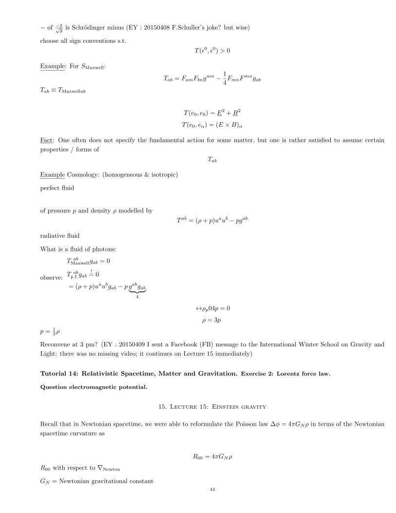
− of −2√g is Schrodinger minus (EY : 20150408 F.Schuller’s joke? but wise)

choose all sign conventions s.t.

T (ε0, ε0) > 0

Example: For SMaxwell:

Tab = FamFbngmn − 1

4FmnF

mngab

Tab ≡ TMaxwellab

T (e0, e0) = E2 +B2

T (e0, eα) = (E ×B)α

Fact: One often does not specify the fundamental action for some matter, but one is rather satisfied to assume certain

properties / forms of

Tab

Example Cosmology: (homogeneous & isotropic)

perfect fluid

of pressure p and density ρ modelled by

T ab = (ρ+ p)uaub − pgab

radiative fluid

What is a fluid of photons:

observe:

T abMaxwellgab = 0

T abp.f.gab

!= 0

= (ρ+ p)uaubgab − p gabgab︸ ︷︷ ︸4

↔ρp04p = 0

ρ = 3p

p = 13ρ

Reconvene at 3 pm? (EY : 20150409 I sent a Facebook (FB) message to the International Winter School on Gravity and

Light: there was no missing video; it continues on Lecture 15 immediately)

Tutorial 14: Relativistic Spacetime, Matter and Gravitation. Exercise 2: Lorentz force law.

Question electromagnetic potential.

15. Lecture 15: Einstein gravity

Recall that in Newtonian spacetime, we were able to reformulate the Poisson law ∆φ = 4πGNρ in terms of the Newtonian

spacetime curvature as

R00 = 4πGNρ

R00 with respect to ∇Newton

GN = Newtonian gravitational constant43

This prompted Einstein to postulate < 1915 that the relativistic field equations for the Lorentzian metric g of (relativistic)

spacetime

Rab = 8πGNTab

However, this equation suffers from a problem

LHS: (∇aR)ab 6= 0

generically

RHS:

(∇aT )ab = 0

thought bubble: = formulated from an action

Einstein tried to argue this problem away.

Nevertheless, the equations cannot be upheld.

15.1. Hilbert. Hilbert was a specialist for variational principles.

To find the appropriate left hand side of the gravitational field equations, Hibert suggested to start from an action

SHilbert[g] =

∫M

√−gRabgab

thought bubble = “simplest action”

aim: varying this w.r.t. metric gab will result in some tensor

Gab = 0

15.2. Variation of SHilbert.

0!= δ︸︷︷︸

gi

SHilbert[g] =

∫M

[δ√−ggabRab︸ ︷︷ ︸

1

+√−gδgabRab︸ ︷︷ ︸

2

+√−ggabδRab︸ ︷︷ ︸

3

]

and 1 : δ√−g =

−(detg)gmnδgmn2√−g

=1

2

√−ggmnδgmn

thought bubbleδdet(g) = det(g)gmnδgmn

e.g. from

det(g) = exp trln g

ad 2: gabgbc = δac=⇒ (δgab)gbc + gab(δgbc) = 0

=⇒ δgab = −gamgbnδgmn

ad 3:∆Rab =︸︷︷︸

normal coords at point

δ∂bΓmam − δ∂mΓmab + ΓΓ− ΓΓ =

= ∂bδΓmam − ∂mδΓmab =

= ∇b(δΓ)mam −∇m(δΓ)mab

=⇒√−ggabδRab =

√−g

“if you formulate the variation properly, you’ll see the variation δ commute with ∂b” EY : 20150408 I think one uses the

integration at the bounds, integration by parts trick

Γi(x) jk − Γi(x) jk are the components of a (1, 2)-tensor.

Notation: (∇bA)ig =: Aij;b44

=⇒√−ggabδRab

=︸︷︷︸∇g=0

√−g(gabδΓmam);b −

√−g(gabδΓmab);m =

√−gAb;b −

√−gBm,m

Question: Why is the difference of coefficients a tensor?

Answer:

Γi(y) jk =∂yi

∂xm∂xm

∂yj∂xq

∂ykΓm(x) ,nq +

∂yi

∂xm∂2xm

∂yj∂yk

Collecting terms, one obtains

0!= δSHilbert =

∫M

[1

2

√−ggmnδgmngabRab −

√−ggamgbnδgmnRab + (

√−gAa) ,a︸ ︷︷ ︸surface

− (√−gBb) ,b︸ ︷︷ ︸

surface term

]

=

∫M

√−gδ gmn︸︷︷︸

arbitrary variation

[1

2gmnR−Rmn] =⇒ Gmn = Rmn − 1

2gmnR

Hence Hilbert, from this “mathematical” argument, concluded that one may take

Rab −1

2gabR = 8πGNTab

Einstein equations

SE−H [g] =

∫M

√−gR

15.3. 3. Solution of the ∇aT ab = 0 issue. One can show (→ Tutorials) that the Einstein curvature

Gab = Rab −1

2gabR

satisfy the so-called contracted differential Bianchi identity

(∇aG)ab = 0

15.4. Variants of the field equations.

(a) a simple rewriting:

Rab −1

2gabR = 8πGNTab = Tab

GN = 18π

Contract on both sides gab

Rab −1

2gabR = Tab||gab

R− 2R = T := Tabgab

=⇒ R = −T

=⇒ Rab +1

2gabT = Tab

⇐⇒ Rab = (Tab −1

2Tgab) =: Tab

Rab = Tab

45

(b)

SE−H [g] :=

∫M

√−g(R+ 2Λ)

thought bubble: Λ cosmological constant

History:

1915: Λ < 0 (Einstein) in order to get a non-expanding universe

>1915: Λ = 0 Hubble

today Λ > 0 to account for an accelerated expansion

Λ 6= 0 can be interpreted as a contribution

− 12Λg to the energy-momentum

“dark energy”

Question: surface terms scalar?

Answer: for a careful treatment of the surface terms which we discarded, see, e.g. E. Poisson, “A relativist’s

toolkit” C.U.P. “excellent book”

Question: What is a constant on a manifold?

Answer:∫ √−gΛ = Λ

∫ √−g1

[back to dark energy]

[Weinberg, QCD, calculated]

idea: 1 could arise as the vacuum energy of the standard model fields

Λcalculated = 10120 × Λobs

“worst prediction of physics”

Tutorials: check that

• Schwarzscheld metric (1916)

• FRW metric

• pp-wave metric

• Reisner-Nordstrom

=⇒ are solutions to Einstein’s equations

in high school

mx+mω2x2 = 0

x(t) = cos (ωt)

ET: [elementary tutorials]

study motion of particles & observers in Schwarzscheld S.T.

Satellite: Marcus C. Werner

Gravitational lensing

odd number of pictures Morse theory (EY:20150408 Morse Theory !!!)

Domenico Giulini

Hamiltonian form Canonical Formulations46

Key to Quantum Gravity

Tutorial 13 Schwarzschild Spacetime

EY : 20150408 I’m not sure which tutorial follows which lecture at this point.

The tutorial video is excellent itself. Here, I want to encourage the use of CAS to do calculations. There are many out

there. Again, I’m partial to the Sage Manifolds package for Sage Math which are both open-source and based on Python.

I’ll use that here.

Exercise 1. Geodesics in a Schwarzschild spacetime

Question Write down the Lagrangian.

Load “Schwarzschild.sage” in Sage Math, which will always be available freely here https://github.com/ernestyalumni/

diffgeo-by-sagemnfd/blob/master/Schwarzschild.sage:

sage: load("Schwarzschild.sage")

4-dimensional manifold ’M’

open subset ’U_sph’ of the 4-dimensional manifold ’M’

Levi-Civita connection ’nabla_g’ associated with the Lorentzian metric ’g’ on the 4-dimensional manifold ’M’

and so on.

Look at the code and I had defined the Lagrangian to be

L

. To get out the coefficients of L of the components of the tangent vectors to the curve, i.e. t′, r′, θ′, φ′, denoted

tp,rp,thp,php

in my .sage file, do the following:

sage: L.expr().coefficients(tp)[1][0].factor().full_simplify()

(2*G_N*M_0 - r)/r

sage: L.expr().coefficients(rp)[1][0].factor().full_simplify()

-r/(2*G_N*M_0 - r)

sage: L.expr().coefficients(php)[1][0].factor().full_simplify()

r^2

sage: L.expr().coefficients(thp)[1][0].factor().full_simplify()

r^2*sin(th)^2

Question There are 4 Euler-Lagrange equations for this Lagrangian. Derive the one with respect to the function

t(λ)!.

sage: L.expr().diff(t)

0

This confirms that ∂L∂t = 0

For ddλ

∂L∂t′ , then one needs to consider this particular workaround for Sage Math (computer technicality). One takes

derivatives with respect to declared variables (declared with var) and then substitute in functions that are dependent upon

λ, and then take the derivative with respect to the parameter λ. This does that:

sage: L.expr().diff( thp ).factor().subs( r == gamma1 ).subs( thp == gamma3.diff( tau ) ).subs( th == gamma3 ).diff(tau)\

....: .factor()

2*(2*cos(gamma3(tau))*gamma1(tau)*D[0](gamma3)(tau)^2 + 2*sin(gamma3(tau))*D[0](gamma1)(tau)*D[0](gamma3)(tau)

+ gamma1(tau)*sin(gamma3(tau))*D[0, 0](gamma3)(tau))*gamma1(tau)*sin(gamma3(tau))

Question Show that the Lie derivative of g with respect to the vector fields Kt :=∂∂t

.

47

The first line defines the vector field by accessing the frame defined on a chart with spherical coordinates and getting the

time vector. The second line is the Lie derivative of g with respect to this vector field.

sage: K_t = espher[0]

sage: g.lie_der(K_t).display() # 0, as desired

0

EY : 20150410 My question is this: ∀X ∈ Γ(TM) i.e. X is a vector field on M , or, specifically, a section of the tangent

bundle, then does

LXg = 0

instantly mean that X is a symmetry for (M, g)? LXg is interpreted geometrically as how g changes along the flow

generated by X, and if it equals 0, then g doesn’t change.

16.

17.

18.

19.

20.

21.

22. Lecture 22: Black Holes

Only depends on Lectures 1-15, so does lecture on “Wednesday”

Schwarzschild solution also vacuum solution (from tutorial EY : oh no, must do tutorial)

Study the Schwarzschild as a vacuum solution of the Einstein equation:

m = GNM where M is the “mass”

g =

(1− 2m

r

)dt⊗ dt− 1

1− 2mr

dr ⊗ dr − r2(dθ ⊗ dθ + sin2 θdϕ⊗ dϕ

in the so-called Schwarzschild coordinates t r θ ϕ

(−∞,∞) (0,∞) (0, π) (0, 2π)

What staring at this metric for a while, two questions naturally pose themselves:

(i) What exactly happens r = 2m?

t r θ ϕ

(−∞,∞) (0, 2m) ∪ (2m,∞) (0, π) (0, 2π)

(ii) Is there anything (in the real world) beyond t→ −∞

t→ +∞

?

idea: Map of Linz, blown up

Insight into these two issues is afforded by stopping to stare.48

Look at geodesic of g, instead.

22.1. Radial null geodesics. null - g(vγ , vγ) = 0

Consider null geodesic in “Schd”

S[γ] =

∫dλ

[(1− 2m

r

)t2 −

(1− 2m

r

)−1

r2 − r2(θ2 + sin2 θϕ2)

]with [. . . ] = 0

and one has, in particular, the t-eqn. of motion:

((1− 2m

r

)t

).= 0

=⇒ (1− 2m

r

)t = k = const.

Consider radial null geodesics

θ!= const. ϕ = const.

From 2 and 2

=⇒ r2 = k2 ↔ r = ±k

=⇒ r(λ) = ±k · λ

Hence, we may consider

t(r) := t(±kλ)

Case A: ⊕

dt

dr=

˙t

r=

k(1− 2m

r

)k

=r

r − 2m

=⇒ t+(r) = r + 2m ln |r − 2m|

(outgoing null geodesics)

Case b. ± (Circle around −, consider −):

t−(r) = −r − 2m ln |r − 2m|

(ingoing null geodesics)

Picture

22.2. Eddington-Finkelstein. Brilliantly simple idea:

change (on the domain of the Schwarzschild coordinates) to different coordinates, s.t.

in those new coordinates,

ingoing null geodesics appear as straight lines, of slope −1

This is achieved by

t(t, r, θ, ϕ) := t+ 2m ln |r − 2m|

Recall: ingoing null geodesic has

t(r) = −(r + 2m ln |r − 2m|) (Schdcoords)49

⇐⇒ t− 2m ln |r − 2m| = −r − 2m ln |r − 2m|+ const.

∴ t = −r + const.

(Picture)

outgoing null geodesics

t = r + 4m ln |r − 2m|+ const.

Consider the new chart (V, g) while (U, x) was the Schd chart.

U︸︷︷︸Schd

⋃ horizon = V

“chart image of the horizon”

Now calculate the Schd metric g w.r.t. Eddington-Finkelstein coords.

t(t, r, θ, ϕ) = t+ 2m ln |r − 2m|

r(t, r, θ, ϕ) = r

θ(t, r, θ, ϕ) = θ

ϕ(t, r, θ, ϕ) = ϕ

EY : 20150422 I would suggest that after seeing this, one would calculate the metric by your favorite CAS. I like the Sage

Manifolds package for Sage Math.

Schwarzschild BH.sage on github

Schwarzschild BH.sage on Patreon

Schwarzschild BH.sage on Google Drive

sage: load(‘‘Schwarzschild_BH.sage’’)

4-dimensional manifold ’M’

/Applications/Sage -6.6. app/Contents/Resources/sage/local/lib/python2 .7/site -packages/sage/geometry/manifolds/utilities.py:283: DeprecationWarning: simplify_radical is deprecated. Please use canonicalize_radical instead.

See http :// trac.sagemath.org /11912 for details.

expr = expr.simplify_radical ()

Levi -Civita connection ’nabla_g ’ associated with the Lorentzian metric ’g’ on the 4-dimensional manifold ’M’

Launched png viewer for Graphics object consisting of 4 graphics primitives

Then calculate the Schwarzschild metric g but in Eddington-Finkelstein coordinates. Keep in mind to calculate the set of

coordinates that uses t, not t:

sage: gI.display ()

gI = (2*m - r)/r dt*dt - r/(2*m - r) dr*dr + r^2 dth*dth + r^2*sin(th)^2 dph*dph

sage: gI.display( X_EF_I_null.frame ())

gI = (2*m - r)/r dtbar*dtbar + 2*m/r dtbar*dr + 2*m/r dr*dtbar + (2*m + r)/r dr*dr + r^2 dth*dth + r^2* sin(th)^2 dph*dph

50

Part 2. Special Relativity

Physics Stackexchange question (from Wesley) and answer (from David Bar Moshe had an excellent question and explana-

tion for special relativity.

http://physics.stackexchange.com/questions/12221/what-does-a-frame-of-reference-mean-in-terms-of-manifolds

Recall that for charts (U, x) ∈ AM(U ′, x′) ∈ AM

, of smooth atlas AM of smooth M . Now x : U ⊂M → Rn

x′ : U ′ ⊂M → Rn

If U ∩ U ′ 6= ∅, by def. of smooth atlas AM , x′ x : Rn → Rn

x x′ : Rn → Rnare diffeomorphisms.

For notation,

A,B ∈ Ω1(M)

A ∧B ∈ Ω2(M)

A ∧B = Aidxi ∧Bjdxj = AiBjdx

i ∧ dxj

A,B ∈ TpM or TM

A ∧B ∈ ∧2(TM), A ∧B = Aiei ∧Bjei = AiBjei ∧ ej(A×B)i = eijkA

jBk or A×B = AjBkεijkei

if dimM = 3, ∗(A ∧B) =√g

(3−2)!AiBjgilgjmεlmndx

n =√ggilAig

jmBjεlmndxn

References

[1] Eric Poisson, A Relativist’s Toolkit: The Mathematics of Black-Hole Mechanics, Cambridge University Press, 2004. ISBN 0 521

83091 5

EY’s references:

[2] Klaus Jnich (Author), S. Levy (Translator), Topology (Undergraduate Texts in Mathematics), Springer; 1st ed. 1984. 2nd Corr. printing

1994 edition (January 1, 1995).

ISBN-13: 978-0387908922

[3] John M. Lee. Introduction to Smooth Manifolds. 2010. Springer. ISBN-10: 0-387-95495-3 (hardcover), ISBN-13: 978-0387-95448-6

E-mail address: ernestyalumni@gmail.com

URL: http://ernestyalumni.wordpress.com ernestyalumni.tilt.com

51