notes for lectures on coherent excitation
TRANSCRIPT

Notes for Lectures on Coherent Excitation
I. RATE EQUATIONS: 2-LEVEL SYSTEM
Consider the 2-level system:
A21
A
FIG. 1: Schematic of two-level system, showing excitation (left) and decay(right).
If we denote the relative populations of levels 1 and 2 by n1 and n2, respectively, then the
equations for the rates of change of these populations are given by:
n1 = n2A + n2BI − n1BI (1a)
n2 = −n2A− n2BI + n1BI (1b)
n1 + n2 = 1. (1c)
The constants A and B are the familiar Einstein A and B coefficients for spontaneous and
stimulated emission/absorption. Here, Bab = π2c2
~ω3∆νAab, (for g1 = g2 = 1), and I is the
intensity of light (in, say, mW/cm2). In order to allow direct use of the more common
laboratory definition of I, the linewidth of the light, ∆ν, has been included in the definition
of B. The first two equations are clearly redundant. Combining the second two equations
we get
n2 = −n2(A + 2BI) + BI. (2)
First, consider the steady-state solution of (2). That is, we set n2 = 0. Then, n2 = BIA+2BI
.
Note that if BI À A, then the steady-state excited population → 1/2.
Now, back to equation (2): Try a solution like n2(t) = f(t) exp[−(A + 2BI)t]. Then,
n2 =[f − f(A + 2BI)
]e−(A+2BI)t. (3)
Setting the right-hand side (RHS) of this expression equal to the RHS of equation (2), and
applying the boundary condition n2(t = 0) = 0, leads to
n2(t) =BI
A + 2BI
(1− e−(A+2BI)t
). (4)
2
Note that as t →∞, n2 → BIA+2BI
, as in the steady-state case.
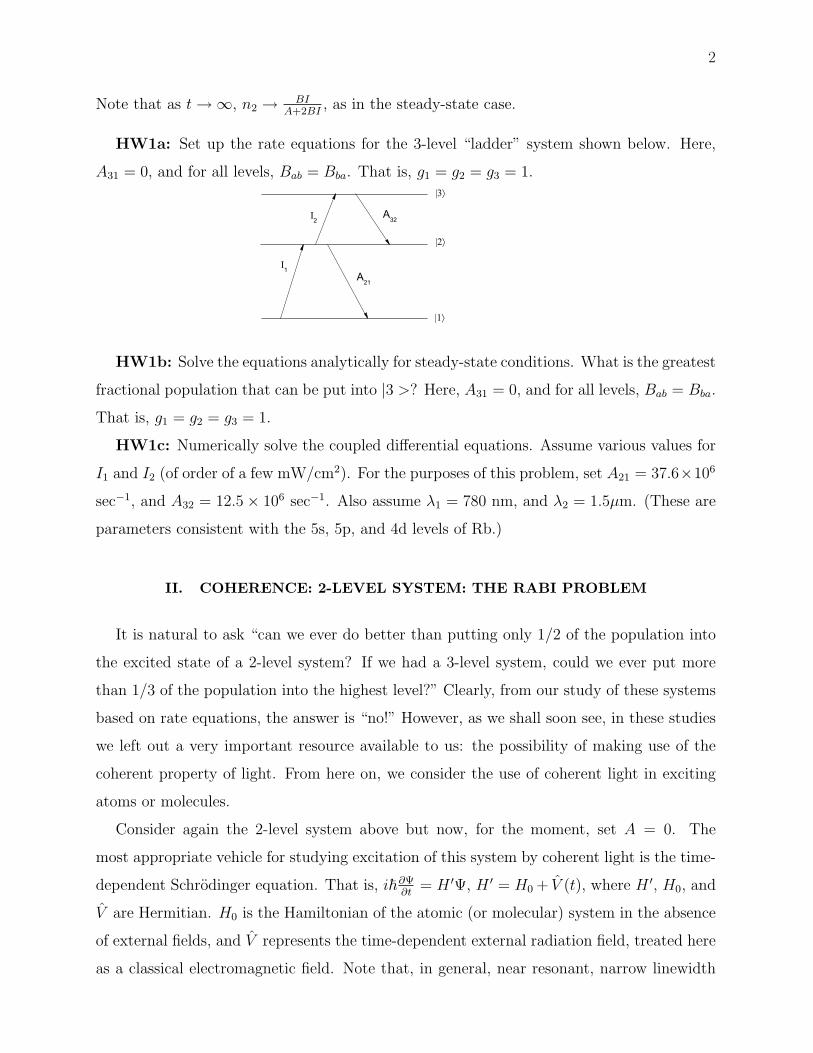
HW1a: Set up the rate equations for the 3-level “ladder” system shown below. Here,
A31 = 0, and for all levels, Bab = Bba. That is, g1 = g2 = g3 = 1.
1A21
2A32
HW1b: Solve the equations analytically for steady-state conditions. What is the greatest
fractional population that can be put into |3 >? Here, A31 = 0, and for all levels, Bab = Bba.
That is, g1 = g2 = g3 = 1.
HW1c: Numerically solve the coupled differential equations. Assume various values for
I1 and I2 (of order of a few mW/cm2). For the purposes of this problem, set A21 = 37.6×10⁶
sec−1, and A32 = 12.5× 10⁶ sec−1. Also assume λ1 = 780 nm, and λ2 = 1.5µm. (These are
parameters consistent with the 5s, 5p, and 4d levels of Rb.)
II. COHERENCE: 2-LEVEL SYSTEM: THE RABI PROBLEM
It is natural to ask “can we ever do better than putting only 1/2 of the population into
the excited state of a 2-level system? If we had a 3-level system, could we ever put more
than 1/3 of the population into the highest level?” Clearly, from our study of these systems
based on rate equations, the answer is “no!” However, as we shall soon see, in these studies
we left out a very important resource available to us: the possibility of making use of the
coherent property of light. From here on, we consider the use of coherent light in exciting
atoms or molecules.
Consider again the 2-level system above but now, for the moment, set A = 0. The
most appropriate vehicle for studying excitation of this system by coherent light is the time-
dependent Schrodinger equation. That is, i~∂Ψ∂t
= H ′Ψ, H ′ = H0 + V (t), where H ′, H0, and
V are Hermitian. H0 is the Hamiltonian of the atomic (or molecular) system in the absence
of external fields, and V represents the time-dependent external radiation field, treated here
as a classical electromagnetic field. Note that, in general, near resonant, narrow linewidth

3
radiation can not be treated as a perturbation.
Set Ψ(t) =∑
n cn(t)ψne−iξn(t), where ψn satisfy the time-independent SE: H0ψn = E0nψn.
The ξn(t) are time-dependent phases. Their values are arbitrary since, being just phases,
they have no effect on any observable.
Then,∂Ψ
∂t=
∑n
ψn
[cn − iξncn
]e−iξn ,
and
H ′Ψ =∑
n
(H0 + V
)cnψne−iξn
Now, V acting on ψ re-distributes the probability. That is,
V ψn = ψ1V1n + ψ2V2n + · · · =∑m
ψmVmn.
Or, upon multiplying from the left by ψ∗q and integrating over space, Vqn = 〈ψq|V |ψn〉 ≡〈q|V |n〉 , where we have made use of the orthonormality of ψ. Then, H ′Ψ =∑
n [cnE0nψn + cn
∑m ψmVmn] e−iξn .
Putting everything together gives
i~∑
n
ψn
[cn − iξncn
]e−iξn =
∑n
cnE0nψne−iξn +
∑n
∑m
cnψmVmne−iξn .
Multiplying through by ψ∗l , and integrating over space gives:
i~∫ ∑
n
ψ∗l ψn
[cn − iξncn
]e−iξnd~r =
∫ ∑n
cnE0nψ
∗l ψne
−iξnd~r+
∫ ∑n
∑m
cnψ∗l ψmVmne−iξnd~r.
Making use of the orthonormality of ψ yields i~(cl − iξlcl
)e−iξl = clE
0l e−iξl +
∑n cnVlne
−iξn , or, i~cl = −~ξlcl + E0l cl +
∑n cnVlne
−i(ξn−ξl).
Finally,
~cl = −i
[(E0
l − ~ξl
)cl +
∑n
cnVlne−i(ξn−ξl)
]. (5)
All of this is exact so far. Now, for the first approximation, we truncate the sum in Eq. (5)
to just the number of levels in the system, here, 2. That is, we neglect the population of
states far from resonance. Under this approximation we end up with:
~c1 = −i[(
E01 − ~ξ1 + V11
)c1 + V12c2e
−i(ξ2−ξ1)]
~c2 = −i[(
E02 − ~ξ2 + V22
)c2 + V21c1e
−i(ξ2−ξ1)],

4
or, more compactly, as:
~c = −i
E0
1 + V11 − ~ξ1 V12e−i(ξ2−ξ1)
V ∗12e
i(ξ2−ξ1) E02 + V22 − ~ξ2
c, (6)
with
c ≡ c1
c2
.
Now, in the dipole approximation, V = −e ~E (~r, t) · ~r, ~E = εE0 (eiωt + e−iωt) /2.
So, Vmn = −e ~E · 〈ψm|~r|ψn〉 = − e2E0 (eiωt + e−iωt) 〈m|r|n〉. Then, defining Ω ≡
−eE0
~ 〈1|r|2〉, we get V12 = ~Ω2
(eiωt + e−iωt). Note that because E0 can, in general, have
a phase term, Ω is, in general, a complex quantity. In many cases we can choose the phase
of our electric field to be 0, in which case, Ω will be pure real.
Equation (6) then becomes:
~c = −i
E1 − ~ξ1~Ω2
(e−i(ξ2−ξ1−ωt) + e−i(ξ2−ξ1+ωt)
)
~Ω∗
2
(ei(ξ2−ξ1−ωt) + ei(ξ2−ξ1+ωt)
)E2 − ~ξ2
, (7)
where E1 ≡ E01 + V11 and E2 ≡ E0
2 + V22.
At this point, we could just solve the coupled differential equations represented by Eq. (7).
First, however, we take advantage of the arbitrariness in the values of the time-dependent
phases, ξn; we assign values to them in such a way as to render Eq. (7) into as simple a form
as possible. That is, we set ξ2 − ξ1 = ωt ⇒ ξ2 − ξ1 = ω.
We now make our third approximation. We say that if a term oscillates at a frequency
significantly higher than the optical frequency, ω , we can ignore that term since it averages
to 0. This is called the rotating wave approximation or RWA. Applying our definitions of
phase, and the RWA to Eq. (7) (whereupon we set terms exp(±2iω) = 0) we obtain:
~c =−i
2
2~∆1 ~Ω
~Ω∗ 2~∆2
c, (8)
where we have defined ~∆1 ≡ E1− ~ξ1 and ~∆2 ≡ E2− ~ξ2 = E2−E1 + ~∆1− ~ω. We can
then set the 0-point of our potential energy scale by setting ∆1 = 0.
Putting all of this together with Eq. (8) we finally obtain
c =−i
2
0 Ω
Ω∗ 2∆2
c, (9)

5
with ~∆2 = E2 − E1 − ~ω. (Throughout these notes I have chosen to use the unfortunate
convention that red detuning is positive, and blue detuning is negative.
The physical picture of this system is:
That is, ~∆2 is the energy by which the laser is detuned from resonance. Because Ω is related
to the electric field amplitude it is, in that sense, related to the laser intensity. However,
since it is also related to the dipole matrix element coupling two states, the value of Ω for
two different transitions are in general different, even if the two laser intensities are identical.
Without going through the (trivial) derivation, Ω is related to more easily obtained system
parameters by:
Ω =
√3λ3Iγ
2πhc, or Ω[MHz] = 1.55× 10⁻⁷
√λ3[nm]I[mW/cm2]γ[s−1],
where γ is the spontaneous decay rate from the upper state. For example, in the case of the
rubidium 5s-5p transition, λ = 780 nm, and 1/γ = 26.6 nsec. Then, for a laser intensity of
1.0 mW/cm2, the Rabi frequency is 21 MHz. Note that Ω is an angular frequency.
Equation (9) is pretty simple, so let’s try to solve it. Breaking up the matrix equation
into its constituent parts, then taking the derivative of each of these we obtain:
c1 =−i
2Ωc2 ⇒ c1 =
−i
2c1 (10a)
c2 =−i
2(Ω∗c1 + 2∆c2) ⇒ c2 =
−i
2(Ω∗c1 + 2∆c2) . (10b)
Combining these equations gives the single, second order differential equation:
c2 + i∆c2 +Ω2
4c2 = 0.
With the boundary condition c2(0) = 0, we can readily show that this has the solution
c2 = −iΩ
Ω′ sinΩ′t2
e−i∆t2 , Ω′ ≡
√Ω2 + ∆2. (11)
Now, the probability of finding the atom in state |2〉 is simply
P2(t) = c∗2c2 =
(Ω
Ω′
)2
sin2 Ω′t2
=Ω2
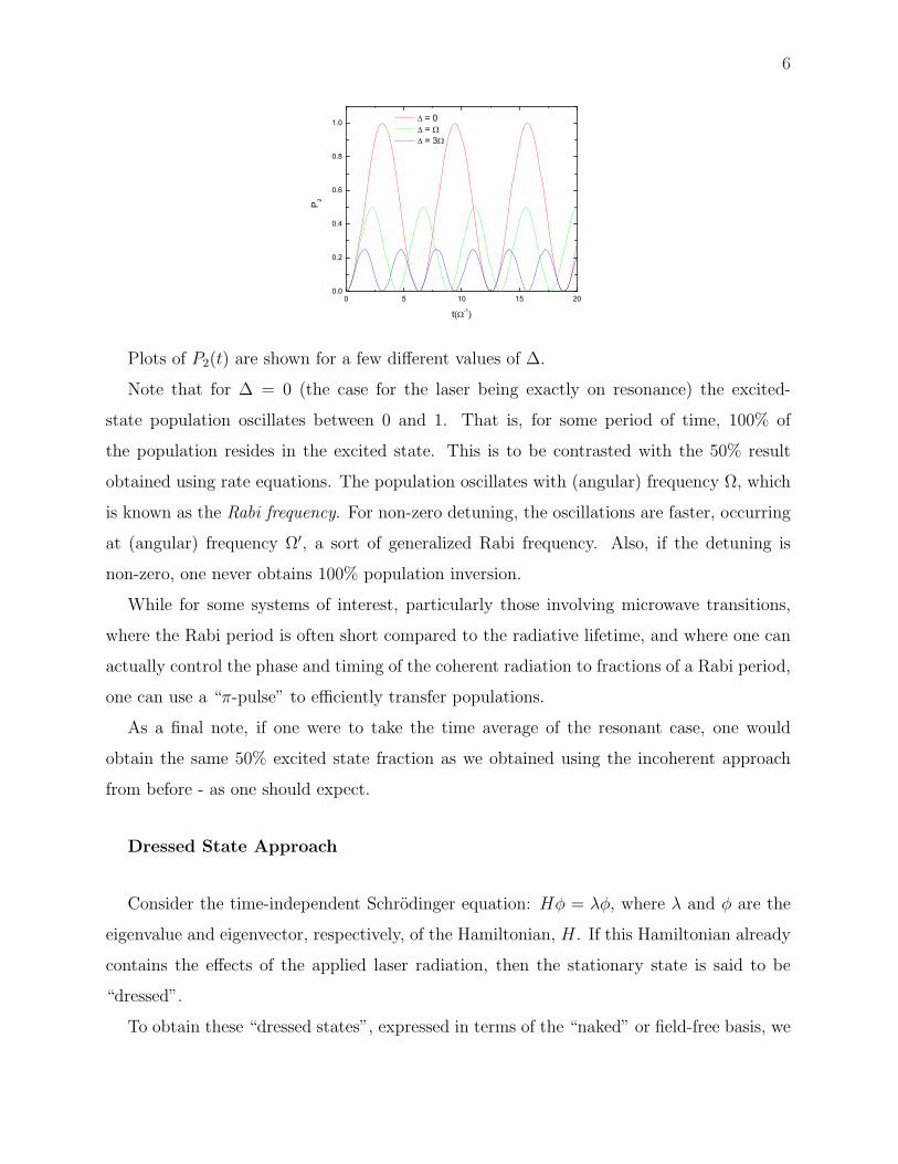
2 (Ω2 + ∆2)(1− cos Ω′t) . (12)
6
0 5 10 15 200.0
0.2
0.4
0.6
0.8
1.0
= 0 = = 3
P2
t( -1)
Plots of P2(t) are shown for a few different values of ∆.
Note that for ∆ = 0 (the case for the laser being exactly on resonance) the excited-
state population oscillates between 0 and 1. That is, for some period of time, 100% of
the population resides in the excited state. This is to be contrasted with the 50% result
obtained using rate equations. The population oscillates with (angular) frequency Ω, which
is known as the Rabi frequency. For non-zero detuning, the oscillations are faster, occurring
at (angular) frequency Ω′, a sort of generalized Rabi frequency. Also, if the detuning is
non-zero, one never obtains 100% population inversion.
While for some systems of interest, particularly those involving microwave transitions,
where the Rabi period is often short compared to the radiative lifetime, and where one can
actually control the phase and timing of the coherent radiation to fractions of a Rabi period,
one can use a “π-pulse” to efficiently transfer populations.
As a final note, if one were to take the time average of the resonant case, one would
obtain the same 50% excited state fraction as we obtained using the incoherent approach
from before - as one should expect.
Dressed State Approach
Consider the time-independent Schrodinger equation: Hφ = λφ, where λ and φ are the
eigenvalue and eigenvector, respectively, of the Hamiltonian, H. If this Hamiltonian already
contains the effects of the applied laser radiation, then the stationary state is said to be
“dressed”.
To obtain these “dressed states”, expressed in terms of the “naked” or field-free basis, we

7
simply solve the eigenvalue equation: H~φ = λ~φ, or
~2
0 Ω
Ω 2∆
φ1
φ2
= λ
φ1
φ2
.
Solving the characteristic equation∣∣∣∣∣∣− λ Ω
Ω 2∆− λ
∣∣∣∣∣∣= 0 ⇒ λ′2 − 2∆λ′ − Ω2 = 0,
or
λ± =~2
(∆± Ω′) . (13)
Then,~2
0 Ω
Ω 2∆
φ1
φ2
=
~2
(∆± Ω′)
φ1
φ2
From whence, φ± = φ0±
(1,
∆± Ω′
Ω
).
We can re-parameterize this expression through the substitutions inspired from the fol-
lowing right triangle:
Then, φ± = φ0±
(1,
cos 2θ ± 1
sin 2θ
)
Normalizing φ gives
φ+ = (sin θ, cos θ) (14a)
φ− = (cos θ,− sin θ) . (14b)
That is,
φ+ = ψ1 sin θ + ψ2 cos θ ⇒ P(+)1 = sin2 θ; P
(+)2 = cos2 θ (15a)
φ− = ψ1 cos θ − ψ2 sin θ ⇒ P(−)1 = cos2 θ; P
(−)2 = sin2 θ, (15b)
where ψ1 and ψ2 are the naked basis eigenvectors.
For example, suppose we start out with the laser greatly detuned to the blue:
(|∆| À Ω, ∆ < 0) or 2θ ≈ π ⇒ θ ≈ π/2. Also, suppose that at t = 0, P1 = 1, and
P2 = 0. This corresponds to the φ+ state, since sin2(π/2) = 1 and cos2(π/2) = 0.

8
If we then adiabatically allow ∆ to move from greatly blue-detuned to greatly red-detuned,
passing through 0-detuning along the way, we will still be in the φ+ state (which is what
we really meant by “adiabatically”) but now we have (|∆| À Ω, ∆ > 0) or 2θ ≈ 0. So,
P1 = sin2(0) = 0, and P2 = cos2(0) = 1. In other words, neglecting spontaneous emission,
we have forced all of the population into the excited state – and without the need for
micro-control of the phase and timing of the radiation.
Note that if we had started out with a red-detuned laser and “chirped” to the blue, we
would have had the same result, but using the φ− state. This process is known by the
seemingly oxymoronic phrase “adiabatic rapid passage”, or ARP.
The following is a plot of P2 versus detuning for a case of ARP. The detuning, measured
in units of Rabi frequency, varies linearly in time from −10Ω to +10Ω.
-10 -8 -6 -4 -2 0 2 4 6 8 10
0.0
0.2
0.4
0.6
0.8
1.0
P2
( )
III. COHERENCE: 3-LEVEL SYSTEMS
Let’s now try to apply the same sort of formalism to 3-level systems. Unlike the 2-level
system, the 3-level system has 3 different basic configurations:
Ladder V
All three configurations have the property that levels 1 and 2 are connected by dipole
matrix elements, levels 2 and 3 are connected by dipole matrix elements, and levels 1 and
3 are not connected by dipole matrix elements. As was the case with the 2-level system,
we shall assume, for the time being, that we can neglect spontaneous emission from any of

9
the levels. We shall also assume that there is no “leakage” into any other state. That is,
probability is conserved within the 3 levels.
In analogy with the 2-level system, we express the electric field of the applied radiation
as
~E(t) = Re(ε1E1e
−iω1t + ε2E2e−iω2t
)=
1
2
[ε1E1
(e−iω1t + eiω1t
)+ ε2E2
(e−iω2t + eiω2t
)].
The εn indicate the polarization of the two electric fields and, as before, Ψ(t) =∑
n cn(t)ψne−iξn(t). Also as before, plugging Ψ(t) into the time-dependent Schrodinger equa-
tion, we obtain again Eq. (5) above,
~cl = −i
[(E0
l − ~ξl
)cl +
∑n
cnVlne−i(ξn−ξl)
].
Now, Vmn = 0 if |n − m| > 1 since, by hypothesis, levels 1 and 3 are not connected.
As before, we approximate the infinite sums by truncating the number of terms to 3, the
number levels in the system. We then obtain the following three equations:
~c1 = −i[(
E01 − ~ξ1 + V11
)c1 + V12c2e
−i(ξ2−ξ1)]
~c2 = −i[(
E02 − ~ξ2 + V22
)c2 + V12c1e
−i(ξ1−ξ2) + V32c3e−i(ξ3−ξ2)
]
~c3 = −i[(
E03 − ~ξ3 + V33
)c3 + V23c2e
−i(ξ2−ξ3)].
Or, in matrix form:
~c = −i
E1 − ~ξ1 V12e−i(ξ2−ξ1) 0
V ∗12e
i(ξ2−ξ1) E2 − ~ξ2 V23e−i(ξ3−ξ2)
0 V ∗23e
i(ξ3−ξ2) E3 − ~ξ3
c, (16)
where, as before, En = E0n + Vnn.
We define the Rabi frequencies as before,
Ω1 =−eE1
~〈1|r|2〉 ⇒ V12 =
~Ω1
2
(e−iω1t + e+iω1t
)
and
Ω2 =−eE2
~〈2|r|3〉 ⇒ V23 =
~Ω2
2
(e−iω2t + e+iω2t
)
With the 3-level systems, the most convenient choice of phases depends on which of the
three systems, ladder, Λ , or V , we are trying to describe. For the ladder system, we choose
ξ2 − ξ1 = ω1t ⇒ ξ2 = ξ1 + ω1,
ξ3 − ξ2 = ω2t ⇒ ξ3 = ξ2 + ω2.

10
For the Λ system, we choose
ξ2 − ξ1 = ω1t ⇒ ξ2 = ξ1 + ω1,
ξ3 − ξ2 = −ω2t ⇒ ξ3 = ξ2 − ω2.
For the V system, we choose
ξ2 − ξ1 = −ω1t ⇒ ξ2 = ξ1 − ω1,
ξ3 − ξ2 = ω2t ⇒ ξ3 = ξ2 + ω2.
Here, we concentrate on the ladder system. Then, applying that choice of phase and
applying the rotating wave approximation, we obtain
~c = −i
E1 − ~ξ1~Ω1
20
~Ω∗1
2E2 − ~ξ1 − ~ω1
~Ω2
2
0~Ω∗
2
2E3 − ~ξ1 − ~ω1 − ~ω2
c,
where now the RWA has allowed us to set terms like e±2iω1t, e±2iω2t, and e±i(ω1±ω2)t all
approximately equal to 0. Note that in this last term, ω1 and ω2 must differ by many Rabi
frequencies for this approximation to be valid. Therefore, the RWA is not strictly valid for
3 equally spaced levels.
We can once again define ~∆1 ≡ E1 − ~ξ1. Then we obtain,
~c = −i
~∆1~Ω1
20
~Ω∗1
2E2 − E1 + ~∆1 − ~ω1
~Ω2
2
0~Ω∗
2
2E3 − E1 + ~∆1 − ~ω1 − ~ω2
c.
We can arbitrarily set the zero-point of our energy to be ~∆1, giving us our final result:
c = − i
2
0 Ω1 0
Ω∗1 2∆2 Ω2
0 Ω∗2 2∆3
c (17)
where we have defined
~∆2 ≡ E2 − E1 − ~ω1 (18a)
11
and
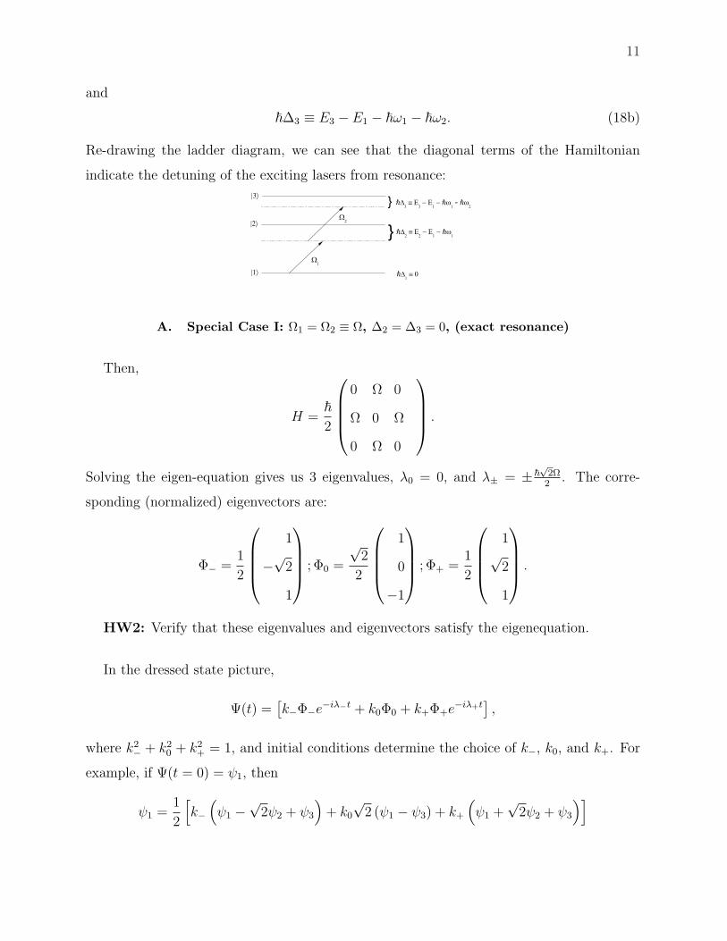
~∆3 ≡ E3 − E1 − ~ω1 − ~ω2. (18b)
Re-drawing the ladder diagram, we can see that the diagonal terms of the Hamiltonian
indicate the detuning of the exciting lasers from resonance:
-
A. Special Case I: Ω1 = Ω2 ≡ Ω, ∆2 = ∆3 = 0, (exact resonance)
Then,
H =~2
0 Ω 0
Ω 0 Ω
0 Ω 0
.
Solving the eigen-equation gives us 3 eigenvalues, λ0 = 0, and λ± = ±~√
2Ω2
. The corre-
sponding (normalized) eigenvectors are:
Φ− =1
2
1
−√
2
1
; Φ0 =
√2
2
1
0
−1
; Φ+ =
1
2
1√
2
1
.
HW2: Verify that these eigenvalues and eigenvectors satisfy the eigenequation.
In the dressed state picture,
Ψ(t) =[k−Φ−e−iλ−t + k0Φ0 + k+Φ+e−iλ+t
],
where k2− + k2
0 + k2+ = 1, and initial conditions determine the choice of k−, k0, and k+. For
example, if Ψ(t = 0) = ψ1, then
ψ1 =1
2
[k−
(ψ1 −
√2ψ2 + ψ3
)+ k0
√2 (ψ1 − ψ3) + k+
(ψ1 +
√2ψ2 + ψ3
)]

12
or,
ψ1
(k−2
+k0√2
+k+
2− 1
)= 0
ψ2
(− k−√
2+
k+√2
)= 0
ψ3
(k−2− k0√
2+
k+
2
)= 0.
From these equations we find k− = k+ = 1/2; k0 =√
2/2. So that
Ψ(t) =1
2
[Φ−e−iλ−t +
√2Φ0 + Φ+e−iλ+t
]
=1
4
[(ψ1 −
√2ψ2 + ψ3
)e+i
√2Ωt2 + 2 (ψ1 − ψ3) +
(ψ1 +
√2ψ2 + ψ3
)e−i
√2Ωt2
]
=1
2
[ψ1
(e+i
√2Ωt2 + e−i
√2Ωt2
2+ 1
)+ ψ3
(e+i
√2Ωt2 + e−i
√2Ωt2
2− 1
)− i√
2ψ2
(e+i
√2Ωt2 − e−i
√2Ωt2
2i
)]
=1
2
[ψ1
(cos
√2Ωt
2+ 1
)+ ψ3
(cos
√2Ωt
2− 1
)− ψ2i
√2 sin
√2Ωt
2
]
= ψ1 cos2
√2Ωt
4− ψ3 sin2
√2Ωt
4− i√
2ψ2 sin
√2Ωt
2.
Therefore,
P1 = cos4
√2Ωt
4; P3 = sin4
√2Ωt
4; P2 =
1
2sin2
√2Ωt
2.
0 5 10 15 20
0.0
0.2
0.4
0.6
0.8
1.0
P1
P2
P3
Pop
ulat
ions
(rel
ativ
e)
t
These results are shown in the above figure where we plot the relative populations of the
3 levels as a function of time, with time in units of the Rabi period, Ω−1. You can see both
from the equations and from the figure that the oscillation frequency for P2 is twice that for
P1 and P3. This is because level 2 gets has “source terms” during both the excitation and
de-excitation of P3.
13
HW3: Calculate the population probabilities as a function of time (for this same degen-
erate case) and for the initial condition Ψ(t = 0) = ψ1, but for Ω1 6= Ω2. For example, set
Ω2 = bΩ1, and plot the populations versus time for b = 0.5, 0, and 2.0.
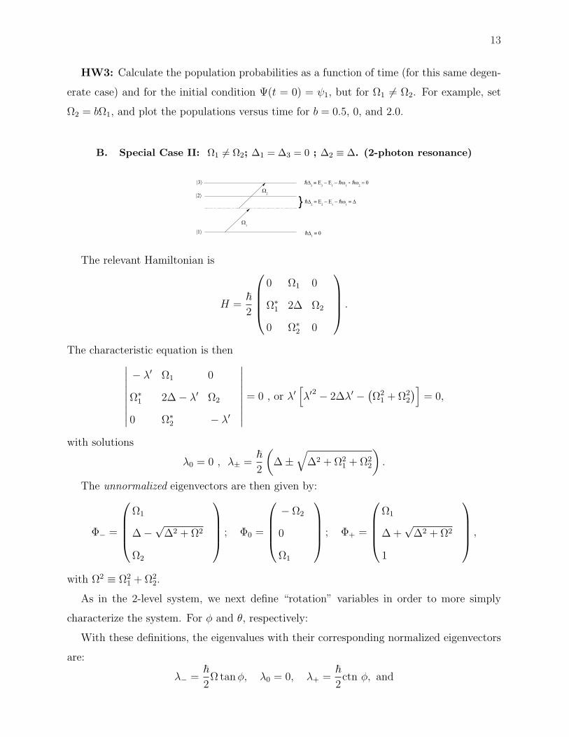
B. Special Case II: Ω1 6= Ω2; ∆1 = ∆3 = 0 ; ∆2 ≡ ∆. (2-photon resonance)
-
The relevant Hamiltonian is
H =~2
0 Ω1 0
Ω∗1 2∆ Ω2
0 Ω∗2 0
.
The characteristic equation is then∣∣∣∣∣∣∣∣∣
− λ′ Ω1 0
Ω∗1 2∆− λ′ Ω2
0 Ω∗2 − λ′
∣∣∣∣∣∣∣∣∣= 0 , or λ′
[λ′2 − 2∆λ′ − (
Ω21 + Ω2
2
)]= 0,
with solutions
λ0 = 0 , λ± =~2
(∆±
√∆2 + Ω2
1 + Ω22
).
The unnormalized eigenvectors are then given by:
Φ− =
Ω1
∆−√
∆2 + Ω2
Ω2
; Φ0 =
− Ω2
0
Ω1
; Φ+ =
Ω1
∆ +√
∆2 + Ω2
1
,
with Ω2 ≡ Ω21 + Ω2
2.
As in the 2-level system, we next define “rotation” variables in order to more simply
characterize the system. For φ and θ, respectively:
With these definitions, the eigenvalues with their corresponding normalized eigenvectors
are:
λ− =~2Ω tan φ, λ0 = 0, λ+ =
~2ctn φ, and

14
Φ− =
sin θ cos φ
− sin φ
cos θ cos φ
, Φ0 =
− cos θ
0
sin θ
, Φ+ =
sin θ sin φ
cos φ
cos θ sin φ
.
Suppose we start out at t → −∞ with Ω2 À Ω1, which means θ → 0. Suppose we
also require that at t → −∞, all of the population is in ψ1. Then, we see that these two
conditions also require that all of the population be in the single dressed state Φ0. Now, if
we adiabatically increase Ω1 and decrease Ω2, we will stay in Φ0, but the entire population
will have moved into ψ3 as Ω2 ¿ Ω1. Note also that because we stay at all times in Φ0, and
because Φ0 never has any component of φ2, no population is ever in ψ2. In the following
two figures, we plot the Rabi frequencies Ω1 and Ω2, and the relative populations of |1〉 and
|3〉 versus time.
0 10 20 30 40 50 60
0.0
0.2
0.4
0.6
0.8
1.0
0 10 20 30 40 50 60
0.0
0.2
0.4
0.6
0.8
1.0
Rab
i Fre
quen
cies
(arb
)
Time (ns)
1
2
5s 5p 4d
Pop
ulat
ion
Time (ns)
Thus, quantum mechanics somehow, “magically” allows us to transfer population from
|1〉 to |3〉, with absolutely no population at any time in |2〉, in spite of the fact that there is
no direct coupling between states |1〉 and |3〉, but strong coupling between both of these and
|2〉! We will now try to, at least qualitatively understand the physics behind this “magic”.

15
Consider a 3-level system in which Ω2 À Ω1. Let the Ω1-field have angular frequency ω,
and the Ω2-field have angular frequency ω2. For the moment, assume these fields are static.
Furthermore, for simplicity we will require ω2 to resonantly couple |2〉 and |3〉, while we
will allow ω to slowly vary with time. Now, because the field associated with the |1〉 to |2〉transition is weak, while the other is strong, we can consider the state of the system to be
well described by Ψ(t) = ψ1c1e−iωt + Φ−B−(t) + Φ+B+(t). That is, we “dress” the upper
states, leaving the lowest state “undressed” or “naked”.
Then, the RWA Hamiltonian describing this system is given by
H(t) =~2
2∆ Ω− Ω+
Ω∗− − 2ε 0
Ω∗+ 0 + 2ε
.
Recall from our treatment of 2-level systems that the 2 states in the “naked” basis, sepa-
rated by an energy E02 −E0
1 are, in the “dressed” basis separated by λ+−λ−. Furthermore,
they are centered about the “0-point” of the potential, and that this 0-point was simply E1.
Thus, in the 3-level system, the dressed states are situated symmetrically about E2, and
are separated by an energy ~Ω2. If we were to scan ω, and measure the absorption of this
light as a function of ω, we would find absorption structure at 2 values of ω, rather than the
single absorption line of the naked system. This dual structure is known as Autler-Townes
splitting and was discovered by Autler and Townes in 1955.
So now let us fix ω so that it would be resonant with the naked basis (placing E1 + ~ω
right at the mid-point of λ1 and λ−. In the naked basis, we would now be exactly 2-photon
resonant with |1〉 → |2〉 → |3〉 excitation. (Actually, we’d be better off if we slightly detuned
ω to, say, the red, and detuned ω2 by the corresponding amount to the blue. But this is
a detail. The key is to be 2-photon resonant.) Now we can see that direct excitation of
|3〉 is possible since we can excite both Φ1 and Φ2, each of which has some |3〉 “character”.
It turns out that if ω really does go to the half-way point between the dressed states,
destructive interference takes place which completely wipes out any population of |2〉. At
this frequency, there is absolutely no absorption of the light associated with ω. That is, the
material becomes completely transparent to the light associated with ω. This condition is
referred to as “Electromagnetically-Induced Transparency” or EIT, and is currently a hot
area of research due to its potential in quantum information applications.

16
Let’s consider a step-by-step analysis (still quantitative) of how this three-level ARP
process works.
1. Only Ω2 is present, dressing the system (except for |1〉). For now, Ω1 is negligible.
2. Now the light associated with Ω1 begins to become important. This light is “scattered”
off the dressed structure, populating |3〉, as described above.
3. Now the light associated with Ω2 begins to drop a bit in intensity, while Ω1 continues
to grow in intensity. Here the population of |3〉 really “kicks in”.
4. The population is now almost completely in |3〉. The intensity of Ω2 is really dropping,
and Ω1 is maximal. So why does the population not revert back to the ground state?
The answer is that there is now nearly no mixing of |2〉 and |3〉 going on, and so the
light associated with ω can’t “talk” to level 3.
5. Finally, the light associated with both lasers is off. In the absence of spontaneous
emission, all the population is trapped in level 3.
IV. DENSITY MATRIX TREATMENT OF COHERENT EXCITATION
I won’t go into much background here. I will only define what we mean by a density
matrix, show that the formalism is equivalent to the time-dependent Schrodinger equation
approach, and then, with no justification at all present you with the prescription for setting
up the “equations of motion” for the system undergoing coherent excitation – but including,
for the first time here, spontaneous emission.
First of all, the density matrix, ρ, is defined as ρij = |ψi〉〈ψj|. Thus, for a 2-level system,
we can write the density matrix as:
ρ =
ρ11 ρ12
ρ21 ρ22
.
Now, the density matrix is Hermitian, meaning that ρij = ρ∗ji. Therefore, the diagonal
elements of the density matrix are real, and in fact represent the populations of the respective
levels. Thus, ρ11 is the population of level 1; ρ22 is the population of level 2, etc. For a

17
conservative system then, Tr[ρ] = 1 (assuming the total population is defined as 1). Note
that since
ρ ≡ |ψ〉〈ψ|,
i~dρ
dt= i~
d|ψ〉dt
〈ψ|+ i~|ψ〉d〈ψ|dt
.
But, the TDSE is
i~d|ψ〉dt
= H|ψ〉 , and− i~〈ψ|dt
= (H|ψ〉)† = 〈ψ|H†.
Then,
i~dρ
dt= H|ψ〉〈ψ| − |ψ〉〈ψ|H†.
or,
i~ρ = Hρ − ρH† ≡ [H, ρ] .
This is the “equation of motion”, or “equation of evolution” for the density matrix.
We can therefore simply solve this equation (or more correctly this system of N equations
for an N-level system) and from the diagonal elements of ρ, write down our populations.
(These are the optical Bloch equations you may have heard of.)
Now, with no derivation or justification at all I present a modification of this equation
of evolution, in which we finally include spontaneous emission. (For details, I refer you to
Shore’s books, listed in the references.)
i~ρij = [H, ρ]ij − i~ [Γρ]ij , with [Γρ]ij ≡ ρij
∑
k
1
2(γik + γjk)− δij
∑
k
ρkkγki.
The γ’s here are simply the decay rates or the Einstein A-coefficients (that we have until now
been designating by ”A”. The use of A is usual in computations using incoherent sources of
light, whereas γ is more commonly used in coherent excitation formulism. In fact, the two
symbols are interchangeable.) In order to simplify the notation, we define γlm = 0 for l ≤ m.
Now at last we’ve got an expression than can truly simulate the “real world” situation in
which spontaneous emission can not always be neglected. Let’s try applying this expression
to the simple 2-level system – including for the first time, realistic decay rates.
Our Hamiltonian and density matrices are:
H =~2
0 Ω
Ω 2∆
and ρ =
ρ11 ρ12
ρ21 ρ22
.
18
where we choose our electric field phases such that the Rabi frequency is pure real. Then,
the commutator is:
[H, ρ] =~2
Ωρ21 − Ωρ12 Ωρ22 − Ωρ11 − 2∆ρ12
− Ωρ22 + Ωρ11 + 2∆ρ21 Ωρ12 − Ωρ21
,
while
Γρ =
− ρ22γ21 ρ12γ21/2
− ρ21γ21/2 ρ22γ21
.
Now, because ρ is Hermitian, ρij = ρ∗ji. Furthermore, in general for any complex number
z = a + ib, with a and b real, z − z∗ = 2ib. Therefore, defining ρij = ρaij + iρb
ij, with ρaij and
ρbij pure real for all values of i, j, we obtain:
ρ =
Ωρb
12 + ρ22γ21 − i (Ωρ22 − Ωρ11 − 2∆ρ12) /2− ρ12γ21/2
cc Ωρb12 − ρ22γ21
.
where “cc” denotes complex conjugate of the 1,2 element. We are solving for the four ele-
ments of ρ. Because it is Hermitian, knowledge of ρ12 tells us ρ21. Furthermore, the diagonal
elements must be pure real, and must sum to 1. Therefore, this expression represents 3 cou-
pled, first order differential equations. In general, for an N-level system, you will have to
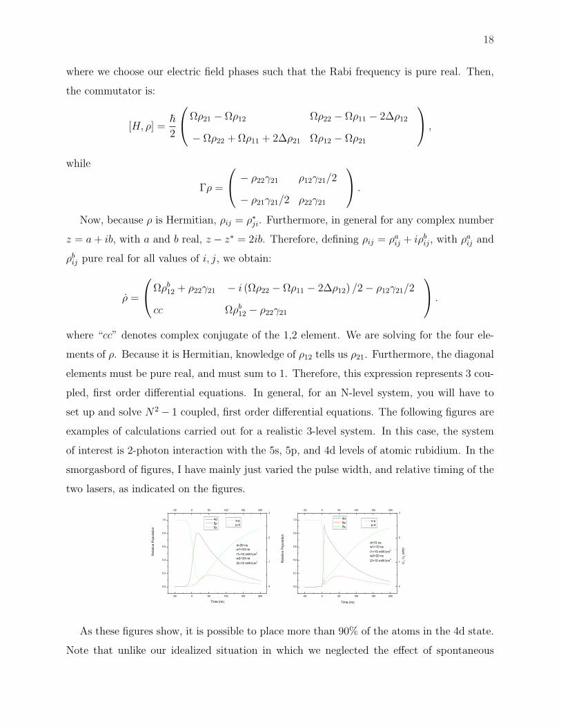
set up and solve N2 − 1 coupled, first order differential equations. The following figures are
examples of calculations carried out for a realistic 3-level system. In this case, the system
of interest is 2-photon interaction with the 5s, 5p, and 4d levels of atomic rubidium. In the
smorgasbord of figures, I have mainly just varied the pulse width, and relative timing of the
two lasers, as indicated on the figures.
-50 0 50 100 150 200
0.0
0.2
0.4
0.6
0.8
1.0
-50 0 50 100 150 200
0
1
2
3
-50 0 50 100 150 200
0.0
0.2
0.4
0.6
0.8
1.0
-50 0 50 100 150 200
0
1
2
3
d=20 nsw1=33 nsI1=10 mW/cm2
w2=33 nsI2=10 mW/cm2
Rel
ativ
e P
opul
atio
n
Time (ns)
4d 5p 5s
s-p p-d
Rel
ativ
e P
opul
atio
n
Time (ns)
4d 5p 5s
d=15 nsw1=10 nsI1=10 mW/cm2
w2=20 nsI2=10 mW/cm2
1, 2 (a
rb)
s-p p-d
As these figures show, it is possible to place more than 90% of the atoms in the 4d state.
Note that unlike our idealized situation in which we neglected the effect of spontaneous

19
-50 0 50 100 150 200
0.0
0.2
0.4
0.6
0.8
1.0
-50 0 50 100 150 200
0
1
2
3
Rel
ativ
e P
opul
atio
n
Time (ns)
4d 5p 5s
d=10 nsw1=10 nsI1=10 mW/cm2
w2=10 nsI2=10 mW/cm2
1, 2 (a
rb)
s-p p-d
emission, the intermediate state, here the 5p, does get populated. This is seen to be es-
sentially exclusively from spontaneous emission from the 4d level, rather than due to direct
excitation from the 5s.
This concludes the “theory” part of the lectures. Next we will consider experimental
efforts to realize these results. We will also discuss applications. None of this will, however,
appear in lecture notes.
V. COHERENT EXCITATION BIBLIOGRAPHY
A. Adiabatic Rapid Passage
Bergmann K., Theuer H., and Shore B. W., Rev. Mod. Phys. 70, 1003 (1998).
Brewer R. G. and Hahn E. L., Phys. Rev. A 11, 1641 (1975).
Coulston G. W. and Bergmann K., J. Chem. Phys. 95, 3467 (1992).
Einwohner T. H., Wong J., and Garrison J. C., Phys. Rev. A 14, 1452 (1976).
Grigoryan G. G. and Pashayan Y. T., Opt. Comm. 198, 107 (2001).
Guerin S., et al., Opt Exp 4, 84 (1999).
Hu X. and Xu Z., J. Phys. B 35, 4527 (2002).
Javanainen J., Phys. Rev. A 46, 5819 (1992).
Kuklinski J. R. et al., Phys. Rev. A 40, 6741 (1989).
Lambert J., Noel M. W., and Gallagher T. F., Phys. Rev. A 66, 053413 (2002).

20
Martin J., Shore B. W., and Bergmann K., Phys. Rev. A 52, 583 (1995).
Morigi G., Franke-Arnold S., and Oppo G.-L., Phys. Rev. A 66, 053409 (2002).
Oreg J., Hioe F. T., and Eberly J. H., Phys. Rev. A 29, 690 (1984).
Oreg J., Hazak J., and Eberly J. H., Phys. Rev. A 32, 2776 (1985).
Oreg J. et al., Phys. Rev. A 45, 4888 (1992).
Radmore P. M., and Knight P. L., J. Phys. B 15, 561 (1982).
Shore, B. W., The Theory of Coherent Atomic Excitation, vols 1 & 2, Wiley 1990.
Sargent M. and Horwitz P., Phys. Rev. A 13, 1962 (1976).
Shore B. W. et al., Phys. Rev. A 44, 7442 (1991).
Shore B. W. et al., Phys. Rev. A 52, 566 (1995).
Stahler M. et al., Opt. Lett. 27, 1472 (2002).
Suptitz W., Duncan B. C., and Gould P. L., JOSA B 14, 1001 (1997).
Vitanov N. V. et al., Advances in Atomic Molecular and Optical Physics 46, B. Bed-
erson and H. Walther, Eds. (Academic, New York, 2001), pp. 55-190 (2001).
Vitanov N. V. et al., Annu. Rev. Phys. Chem., 52, 763 (2001).
Vitanov N. V., Shore B. W., and Bergmann K., Eur. Phys. J. 4, 15 (1998).
B. Electromagnetically Induced Transparency
Badger S. D., Hughes I. G., and Adams C. S., J. Phys. B 34, L749 (2001).
Boon J. R. et al., Phys. Rev. A 57, 1323 (1998).
Boon J. R. et al., Phys. Rev. A 59, 4675 (1999).
Cataliotti F. S., Phys. Rev. A 56, 2221 (1997).
Chen H. X. et al., Phys. Rev. A 58, 1545 (1998).

21
Clarke J., Chen H. X., and van Wijngaarden W. A., Appl. Opt 40, 2047 (2001).
Fleischhauer M., and Lukin M. D., Phys. Rev. Lett. 84, 5094 (2000).
Fulton et al., Phys. Rev. A 52, 2302 (1995).
Gea-Banacloche J. et al., Phys. Rev. A 51, 576 (1995).
Greentree A. D. et al., Phys. Rev. A 65, 053802 (2002).
Harris S. E. and Yamamoto Y., Phys. Rev. Lett. 81, 3611 (1998).
Imamoglu A. Phys. Rev. Lett. 89, 163602 (2002).
Li Y. and Xiao M., Phys. Rev. A 51, 4959 (1995).
Li Y. and Xiao M., Phys. Rev. A 51, R2703 (1995).
Lukin M. D. et al., Phys. Rev. Lett. 79, 2959 (1997).
Marangos J. P., J. Mod. Opt. 45, 471 (1998).
McCullough E., Shapiro M., and Brumer P., Phys. Rev. A 61, 041801 (2000).
Rocco A. et al., Phys. Rev. A 66, 053804 (2002).
Schmidt H., and Imamoglu A., Opt. Lett. 21, 1936 (1996).
Shepherd S., Fulton D. J., and Dunn M. H., Phys. Rev. A 54, 5394 (1996).
Xiao M. et al., Phys. Rev. Lett. 74, 666 (1995).
Yan M., Rickey G., and Zhu Y., JOSA B 18, 1057 (2001).
C. Super-/Sub-Luminal Propagation of Light
Budker D. et al., Phys. Rev. Lett. 83, 1767 (1999).
Dutton Z. et al., Sci. 293, 663 (2001).
Harris S. E., Field J. E., and Kasapi A., Phys. Rev. A 46, R29 (1992).

22
Hau L. V. et al., Nat. 397, 594 (1999).
Kash M. M. et al., Phys. Rev. Lett. 82, 5229 (1999).
Liu C. et al., Nat. 409, 490 (2001).
Lukin M. D. and Imamoglu A, Nat. 413, 273 (2001).
Mair A. et al., Phys. Rev. A 65, 031802 (2002).
Milonni P. W., J. Phys. B 35, R31 (2002).
Phillips D. F. et al., Phys. Rev. Lett. 86, 783 (2001).
Wang L. J., Kuzmich A., and Dogariu A., Nat. 406, 277 (2000).
Zibrov A. S. et al., Phys. Rev. Lett. 76, 3935 (1996).