notes for chaos and fractals - john boccio website

Notes for Chaos and Fractals

John R. BoccioProfessor of PhysicsSwarthmore College

April 26, 2012

Contents

1 Chaos 11.1 What is Chaos? . . . . . . . . . . . . . . . . . . . . . . . . . . . . 1

1.1.1 Revolution . . . . . . . . . . . . . . . . . . . . . . . . . . 101.1.2 Studying Chaos . . . . . . . . . . . . . . . . . . . . . . . . 101.1.3 First Pass on Ideas about Difference Equations or Life’s

Ups and Downs . . . . . . . . . . . . . . . . . . . . . . . . 151.1.4 Some Thoughts . . . . . . . . . . . . . . . . . . . . . . . . 20

1.2 Approach to Chaos . . . . . . . . . . . . . . . . . . . . . . . . . . 221.2.1 Introduction . . . . . . . . . . . . . . . . . . . . . . . . . 22

1.3 Introduction to Dynamic SystemsToward an Understanding of Chaos . . . . . . . . . . . . . . . . . 28

1.4 More Details . . . . . . . . . . . . . . . . . . . . . . . . . . . . . 401.5 Expanding these ideas . . . . . . . . . . . . . . . . . . . . . . . . 52

1.5.1 The Bifurcation Diagram . . . . . . . . . . . . . . . . . . 521.5.2 Sensitivity to Initial Conditions . . . . . . . . . . . . . . . 531.5.3 Symptoms of Chaos . . . . . . . . . . . . . . . . . . . . . 561.5.4 Two- and Three-Dimensional Systems . . . . . . . . . . . 561.5.5 The Predator-Prey System . . . . . . . . . . . . . . . . . 571.5.6 Continuous Functions and Differential Equations . . . . . 591.5.7 Types of two-dimensional interactions . . . . . . . . . . . 601.5.8 The buckling column system . . . . . . . . . . . . . . . . 601.5.9 Basins of attraction . . . . . . . . . . . . . . . . . . . . . 621.5.10 Three-dimensional Dynamic Systems - The Lorenz System 631.5.11 Beasts in Phase space - Limit Points . . . . . . . . . . . . 64

1.6 The Nonlinear Damped Driven Oscillator . . . . . . . . . . . . . 641.6.1 Zooming in . . . . . . . . . . . . . . . . . . . . . . . . . . 76

1.7 Appendix . . . . . . . . . . . . . . . . . . . . . . . . . . . . . . . 821.7.1 Stability of Fixed Points . . . . . . . . . . . . . . . . . . . 821.7.2 Generating the Lyapunov Exponent Curve . . . . . . . . 83

2 Fractals 852.1 Introduction . . . . . . . . . . . . . . . . . . . . . . . . . . . . . . 852.2 The Nature and Properties of Fractals . . . . . . . . . . . . . . . 882.3 The Concept of Dimension . . . . . . . . . . . . . . . . . . . . . . 89

i

ii CONTENTS

2.3.1 The Hausdorff Dimension . . . . . . . . . . . . . . . . . . 912.3.2 The length of a coastline . . . . . . . . . . . . . . . . . . . 922.3.3 The Cantor Set . . . . . . . . . . . . . . . . . . . . . . . . 932.3.4 The Koch Snowflake . . . . . . . . . . . . . . . . . . . . . 952.3.5 Sierpinski Triangle . . . . . . . . . . . . . . . . . . . . . . 972.3.6 IFS Fractals . . . . . . . . . . . . . . . . . . . . . . . . . . 100

2.4 Fractal Dimension Program . . . . . . . . . . . . . . . . . . . . . 1022.5 Complex Maps . . . . . . . . . . . . . . . . . . . . . . . . . . . . 108

2.5.1 Mandelbrot Sets . . . . . . . . . . . . . . . . . . . . . . . 1092.6 So what is a fractal? . . . . . . . . . . . . . . . . . . . . . . . . . 111

2.6.1 Why do we care about fractals? . . . . . . . . . . . . . . . 1112.7 Final Example - The Cube Roots of 1 . . . . . . . . . . . . . . . 111

Chapter 1

Chaos

1.1 What is Chaos?

Let us make a first, quick pass over many ideas related to the subject of chaos.We will cover all of these ideas again in more detail later in these notes. Ourfirst pass is desgined to let us see the big picture.

Let me first illustrate(in class) some real systems, namely the chaotic calculatorand the Barnsley game. Both will seem like silly exercises, but we will see laterthat there is very deep stuff happening in these systems.

The irregular aspects of nature, the discontinuous or erratic side, such as frac-tal structures I will illustrate in class, or the behavior of simple equations suchas the logistic map, the roots of three, the Mandelbrot set, or the Lorenz map(we will illustrate these in class), have always been regarded as puzzles or evenmonstrosities; this also includes things like turbulence, fluctuations, etc.

These phenomena were always regarded as hopelessly ”chaotic” (without anyunderstanding of the meaning of the term) and thus, not possible to understand.

The study of chaos has heavily used computer calculations and computer graph-ics in an effort to better understand the underlying complexities; we will usethem to demonstrate various phenomena in this class and to run simulations.

All kinds of new words and a new language has appeared such as fractals, bi-furcations, limit cycles, attractors, etc - we will attempt to understand them alland learn to ”speak” this language.

Chaos seems (now) to be everywhere - smoke swirls, flag waving, drippingfaucets, cars on a highway, fluid flow, etc.

1

All of these phenomena are seemingly very different, but, as we will see, theyall obey the same set of new laws.

Chaos is a science of the GLOBAL nature of systems - it crosses over thetraditional boundaries between disciplines and to understand it we will need tomix disciplines.

The studies we will be carrying out will show that one needs less specializationin education - specialized training is too narrow to deal with the systems wewill investigate. I do not mean to imply that one should not have extensiveknowledge of a field - what I am saying is that your training should encompassmore than one field(in depth).

Accepted methods will fail ........

Complex, chaotic systems have universal(common) aspects - universality willappear.

Scientistis that study chaos look for patterns, especially patterns that are inde-pendent of scale - they explore randomness and complexity, jagged edges andsudden changes(discontinuities).

Relativity eliminated the Newtonian illusion of absolute space and time- that space and time were independent.

Quantum Mechanics eliminated the Newtonian dream of a controllablemeasurement process.

Chaos, as we will see, eliminates the Laplacian fantasy of deterministicpredictability.

The mainstream study of physics in the past century has really been the studyof the ”building blocks of matter”. At higher and higher energies the in-vestigations correspond to smaller and smaller scales and to shorter and shortertimes - the hope is to find the ultimate building blocks (fundamental entities)with which everything else can be built. We note there has been only slow,excruciating progress( if any) for decades.

Suppose that we did understand the fundamental laws or rules (hopefully theywill be simple rules at the lowest level) of nature. This leaves unanswered, how-ever, the question of how to apply the rules to anything beyond the most simplesystems involving only a few particles. One wonders how they might be appliedto a bathtub full of water or the weather, etc.

The physics developed in the 20th century, which has often been described asa search for the theory of everything, cannot even be used to answer the mostfundamental questions about nature - How did life begin? What is turbulence?

2

How does order arise? and so on.

Even phenomena thought to be well understood (simple fluids, mechanical sys-tems like the pendulum, etc) were not understood, as we will see!

The simplest systems, once assumed to be completely understood, have extraor-dinarily complex behavior related to unpredictability.

When we look (investigate) carefully, however, a new kind of order arises spon-taneously(emerges) in these systems - chaos and order intermingled.

Traditionally, when physicists saw complex results, they looked for complexcauses, i.e., the turbulence at the bottom of a waterfall is a good example -one might ask the question - what causes the complex, turbulent behavior atthe bottom of the waterfall? It seemed clear to traditional physicists that thebottom of the waterfall required a very complex theory for its understand - itdoes not!

If physicists saw a random relationship between input and output for a system,then they would build into the theory some randomness by artificially addingnoise or error to their initial conditions. This was the wrong approach.

What is the correct way?

Let us look at some simple (mathematical and physical) systems (a first passwith more later). We will find in all cases that very small input(initial) differ-ences can lead to what we will call chaotic output differences. We will find thatsimple equations (laws or rules) lead to the turbulence(chaotic behavior) at thebottom of a waterfall.

Let us begin by talking about something that you have probably heard about -the butterfly effect.

Long ago, many meteorologists thought that weather forecasting was a lot ofguesswork and helped by experience. They also felt that the computer with itsability to crunch numbers very fast, would allow then to prove the Newtonianidea that the weather follows a deterministic path - like planets, comets, eclipses,tides, etc, i.e., that we could make predictions from known initial conditions andknown physical laws even if the the system was complex.

We should be able to make weather calculations so accurate that they will ef-fectively be forecasts. The weather is complicated, but is is governed by knownlaws. Thus, a powerful computer with accurate initial conditions should be ableto make forecasts.

This was the view of science in the 1960’s. There was one small fly in the

3

ointment, however. We would need to know the initial conditions EXACTLY.This might be done with a grid of measuring instruments all over the surface ofthe earth, on/under the oceans, in the atmosphere, etc.

In actuality, however, this can only represent approximate initial conditionssince sensors cannot be everywhere. Science, however, has always assumed thatapproximate initial conditions imply approximate behavior of the system, i.e.,if we have small errors or a set of sensor data that is, for all practical purposes,complete, then we can neglect the small errors or small amounts of missing data- it was thought that arbitrarily small influences (that might be missed) do notgenerate arbitrarily large effects!

This always worked and was firmly believed to be true in all systems - ap-proximate (to some degree) input always give approximate(to the same degree)output!

In 1963, a strange thing happened while Edward Lorenz was working on hisweather model. He was running a computer simulation using his model andafter many days, when it was just beginning to get interesting, the computercrashed. Suppose one of the weather variables he was calculating looked likethe graph below (as a function of time).

time

Weather Variable

start

crash

Figure 1.1: Lorenz Computer Model - Run 1

He then did the ”standard thing”. He looked at the printouts and used thedata from some time before the computer crash to restart the simulation. Thevalues he used for the initial conditions were accurate to 6 decimal places andhe assumed that the simulation would be identical up to the crash and then allnew calculations would be the same as if the first run had not crashed.

This, however, was not what happened. As shown in the graph below

4

time

Weather Variable

start

crash

restart

new run

Figure 1.2: Lorenz Computer Model - Run 2

the second run was identical to the first run for a short time but then deviatedand after some time they were totally different - the weather behavior at largetimes for the two runs did not resemble one another in any way!

The initial values for the second run could only have been in error by 1 partin 1,000,000 and this should not have led to such a dramatic deviation in theresults.

When using a completely deterministic system of equations with approximateinitial conditions, it was thought that slight differences scattered around shouldcancel out and thus have no significant effect on large scale features of theweather - but in actuality one observes catastrophic differences in such systems,as seen above.

Therefore, while the equations do imply a weather prediction that probablyoccurs somewhere at some time, it is likely that it is not where and when themodel predicts, thus implying that any form of prediction is doomed! It seemsthat any physical system that has non-periodic behavior will be unpredictable.Again we can see this in a class demo of the Lorenz effect with many startingpoints.

The phenomenon is called the butterfly effect.

The sensor grid with missing values hides fluctuations and leads to approximateinitial conditions. No prediction is possible - a butterfly might have flapped itswings in a gap!

It seemed that predictability was giving way to randomness (no predictability).

The Lorenz results, however, seemed to imply more than randomness. They

5

seemed to imply some kind of geometrical structure at a fine scale - some kindof order masquerading as randomness.

This led to studies of so-called aperiodic systems or systems that almost re-peated themselves but never quite succeeded. These studies implied that theremust be a link between aperiodicity and unpredictability.

The butterfly effect is no accident! The studies implied that it is necessary,i.e., suppose that small perturbations remain small instead of generating theobserved chaotic effects. This would imply that when the weather came arbi-trarily close to a state it had passed earlier, it would stay arbitrarily close to allthe patterns that followed that earlier state. This means that we could predictfuture weather patterns and cycles, which we cannot - thus, the butterfly effectmust exist!

The butterfly effect is equivalent to sensitivity to initial conditions.

But how does it happen? How could such unpredictability - such chaos - arisefrom a simple deterministic system of equation(there were 12 equations in theLorenz weather model). The simpler Lorenz model I have been using for il-lustrations has only three equations. They are non-linear equations (we willdefine them in detail later). Non-linear equations are not generally soluble an-alytically. All real systems are non-linear although the non-linear terms wereusually neglected (assumed to be small effects that that would not influencelarge scale behavior) - thus, the butterfly effect was removed from the modelsand everyone was surprised when it appeared!

Let us look at a simple example model - the Lorentzian water wheel as shownbelow.

●

⇊

Figure 1.3: Lorentzian Water Wheel

6

As shown, we have a wheel that can rotate in either direction. Buckets areattached to wheel. Water flows into a bucket at the top and the buckets leakwater. The steady flow of water into the buckets correspond to energy inflowinto the system - it means that the system is driven by an external system(supplies the water). The leakage of water means that the system is losingenergy also - this is called dissipation.

Case #1: The rate of inflow is very low. This implies that the top bucketnever fills up. Thus there is no movement.

Case #2: We have a slightly faster rate of inflow until steady motion setsin (corresponds to net torque =0 and all water leaked out by time bucketsreaches the bottom).

Case #3: If inflow rate is increased, the rotational motion becomes chaotic- due to non-linear effects that have been built into the system - the rateof spin is proportional to the amount of inflow into the bucket which isproportional to the spin and so on....i.e., if the spin is large, buckets havelittle time to fill up - also buckets can pass the bottom and start up thesides before emptying. This causes a slowing down and possibly a reversalof the spin direction. In fact, over long periods, the spin reverses manytimes, never settling down to any kind of steady-state and never repeatingitself in any predictable manner.

A pre-chaos physicist’s intuition would imply that over the long term - if therate never varied - a steady-state would evolve, i.e, either the wheel would rotatesteadily or it would oscillate steadily back and forth at constant intervals.

But that is not what is observed for this system. To understand the observationsand to hint at future discussions consider the following ideas.

We assume the system has three equations and three variables. To visualizehow the system evolves in time we could plot each variable as a function of time(called a time series) as shown below.

t

V1

Figure 1.4: 1 Variable Time Series

7

Alternatively we could plot the evolution in a 3-dimensional space as shownbelow (called a phase space).

V1 V2

V3

Figure 1.5: 3 Variable Phase Space

Here the path also represents how the variables are changing with time - eachpoint on curve corresponds to a given time t and the point has coordinates(V1(t), V2(t), V3(t)).

The meanings of different types of paths in phase space are as follows: If thepath stops at a point, this corresponds to the variables remaining constant ora steady-state situation. If the path loops (closed path), then this implies aperiodic (repeating) motion.

Some examples are;

x

Vx

time

steady-state(rest)

Figure 1.6: Particle with friction

8

x

Vx

Figure 1.7: Simple periodic motion

x

Vx

Figure 1.8: Not so simple periodic motion

What did Lorenz see?

He saw no steady states and no loops implying periodicity. He only saw whathe called infinite complexity. In particular, he found that

1. The path stayed in a finite volume (within well-defined bounds).

2. The path never repeated itself.

3. The path traveled along a strange, distinctive shape - a kind of doublespiral in 3D space (like a pair of butterfly wings (as we saw earlier)). Thisimplied pure disorder, since no points ever repeated!

However, it contained a new kind of order.

Why didn’t scientists see this ”chaos” if it was everywhere? It was becausetypical scientific training leads to narrow, discipline oriented studies - to com-partmentalized knowledge. Each discipline has its own narrow methods applica-ble beautifully to the problems of that particular discipline. Each discipline alsotends to ignore problems that cannot be solved using their standard approachesand methods. They were not seeing a large, cross-disciplinary picture! But itwas there and was seen by Lorenz!

9

1.1.1 Revolution

Science is not an orderly process. It does not progress by simple accretion ofknowledge. Most scientists are not innovators, but only solvers of puzzles. Theproblem is that in order to advance in one’s discipline, the puzzles that oneattempts to solve are the ones they believe can be stated and solved within theconventional wisdom of the field (the so-called orthodox approach).

Then there are revolutions.

Revolutions lead to new science.

Revolutions usually occur when scientists cross boundaries (of the disciplines).

Revolutions usually use ”illegitimate” or ”unorthodox” modes of inquiry.

This is what happened in the study of chaos ... the early investigators wereshunned, ridiculed, ......

Chaos has become more than a theory and more than a set of beliefs. It has itsown technique of using computers via flexible interaction, i.e.,

mathematic becomes an experimental science

computers replace laboratories

computer graphics becomes important because of the unique ability of thehuman eye-brain interface to synthesize.

1.1.2 Studying Chaos

What can we study to see chaos?

What about the rock of Gibraltar of deterministic physics, namely, the pendu-lum, which is the prime example of constrained action, the epitome of clockworkregularity. Of course, no ”real”, ”top-ranked”, physicist would have botheredto study the pendulum in the 20th century - it was completely understood - itwas the classic deterministic system.

But that was a mistake. For within the study of the pendulum were some hid-den surprises - hidden because the standard investigatory methods were notdesigned to looked for them!

Certainly, there is amazing regularity (predictability) in the pendulum system,but investigators saw that easily in many experiments because that is whattheir approximate theories predicted - the approximate theory was powerful -so powerful that it saw a regularity that does not exist.

10

Maybe experimentalists should not know the theory prior to doing experiments!

A better theory, i.e., one that includes some non-linearity due to the size of theinitial displacement angle leads to some irregularities; scientists, however, as-sumed that small non-linear inputs would only lead to small output effects!

To get an absolutely regular system, we must ignore all non-linearities in thesystem. We must ignore, friction, air resistance and not displace the systemfrom its rest position (equilibrium) very much.

In the real world, however, pendulums do not remain regular - they stop. Thetwo figures below (in phase space) illustrate this dilemma.

Figure 1.9: Periodic, regular motion

steady-state(rest)

Figure 1.10: Real motion

Dissipative systems change and this defeats regularity. On top of this, othernon-linear effects lead to systems that are not solvable exactly(analytically) -they can be approximated if the non-linearities are small, but that defeats theinvestigation of realistic systems.

No one suspected chaos lurked around if the non-linearities were included totheir full extent - no one even looked!

Think of something you are familiar with, namely a playground swing. If you

11

give the swing a push, it oscillates but quickly damps out, coming back to restunless it is driven (you keep pushing). It turns out that its motion can (in thelong term) be regular (you keep pushing at a regular rate but not too strong)or it could be erratic, never settling down to a steady-state - never exactly re-peating any previous motion (you keep pushing at a regular rate but now muchstronger pushes).

It turns out that unpredictability was not the reason these systems became in-teresting. This disorderly behavior of simple systems implies a creative processis taking place. This process generates complexity - this corresponds to richlyorganized patterns - sometimes stable and sometimes unstable - sometime finiteand sometime infinite - but always fascinating.

Consider the toy demo of a magnetic chaotic pendulum(+simulation) in class.It consists of a magnet at the end of a pivoted rod (a spherical pendulum) andthree magnets on the base (carefully positioned at the corners of an equal sidestriangle). We now do a series of repeated experiments.

We start the pendulum off somewhere (arbitrary) and see where it ends up (atone of the three magnets (attractive)) on the floor. Call the three floor magnets(red, blue, green). We then color the starting point with the color of the finalmagnet position. What does the colormap look like? Old style, non-chaos, non-complexity thinking, would answer - three regions- red nearest the red magnet,blue nearest the blue magnet and green nearest the green magnet with sharpboundaries as shown below.

RED

BLUE

GREEN

Figure 1.11: Deterministic Guess

That is not what is observed however. We do get regions of solid color, which

12

means that the pendulum magnet reliably goes to the magnet of that color.But we also get regions where the colors are woven together with infinite com-plexity, i.e., adjacent to red point, no matter how close you choose to look, nomatter how much you magnify the map, there will be green and blue points.This implies, that for all practical purposes (would need infinitely accurate ini-tial conditions) the pendulum magnet’s destiny is impossible to predict! Someillustrations are shown below.

Figure 1.12: The experimental results

Figure 1.13: The boundary expanded

13

Figure 1.14: The boundary expanded further

We will discuss the details of these patterns later (they will arise from a com-pletely different and strange source).

The traditional physicist would write down the appropriate equations includingangles, friction, driving forces, etc (including all the nonlinearities) and get anunsolvable system. They would then turn to the computer to simulate the sys-tem. They repeat the calculation many times generating the color map. Greatcare must be exercised since computers have a bit-range problem and if thesimulation is run long enough one obtains only noise.

Is there anything hidden in this seeming unpredictability?

Is there any pattern? Is there any structure in the seemingly random behavior?

Physicists seemed to be able to understand the short term motion of the sys-tem, but could not extend that understanding to the long term motion whennon-linearities were present.

The microscopic (fundamental equations or rules) pieces are clear, but themacroscopic behavior (complex patterns) remained a mystery!

The tradition of looking at systems locally - isolating small scale mechanisms -and then adding the local effects together to figure out the whole system - wasbeginning to break down.

The standard method of reductionism where we understand the smallest build-ing blocks and build the larger system up from the behavior of the smaller blockswas failing.

14

The whole seemed to be more than a sum of its parts!

Knowledge of the fundamental equations no longer seemed to be the right kindof knowledge at all.

Physicists had to learn again - had to learn to see things that they had learnednot to see!

Chaos and instability are not the same at all!

A chaotic system could be stable (means equilibrium) if its type of irregularitypersisted in the face of small disturbances (the traditional definition of equilib-rium).

The chaos of the pendulum is as stable as the equilibrium of a marble sitting atthe bottom of a bowl!

You can add noise, jiggle it, stir it up, interfere with the motion and then wheneverything has settled down - the transients(due to our messing around) dyingaway - the system returns to the same peculiar pattern of irregularities as be-fore.

The system is locally unpredictable, but globally stable.

Real dynamical systems play by a more complicated set of rules then anyonehad imagined.

The idea that systems behave in certain quantitative ways that depend noton the detailed physics or model description, but rather only on some generalproperties of the system is called universality.

1.1.3 First Pass on Ideas about Difference Equations orLife’s Ups and Downs

Traditionally, physicists study a problem, develop relevant equations with vari-ables that are continuous functions of time (called differential equations) andtry to make predictions. They often cannot solve the equations analytically,so they turn to computers. The numerical computer solutions return answersat discrete values of the time variable (not continuous values) and one simplyassumes continuity, i.e., nothing strange happens between the closely space dis-crete time values and we can connect them with continuous curves.

Biologists, on the other hand, use experiment to study systems. They gener-ate equations that give output matching the data from the experiment. Theirvariables, parameters, driving forces, etc are very complicated and they mustidealize the equations. This works in the sense that if the mathematical model

15

had certain types of behavior, then this implied that one could usually guesscircumstances where real systems would behave the same way.

Experimental data naturally comes at discrete time intervals (not continuous).Equations relating variables known only at discrete time values are called differ-ence equations. In these equations, the process jumps from state to state withno knowledge about ”in between”.

This is saying that, in these systems, changes at discrete intervals are moreimportant than what is happening at every time point (more important thancontinuity).

In these equations, a variable now depends only on the variable(s) last year(lastmonth,.....) i.e.,

xnext = f(xnow)

orxn+1 = f(xn)

In such a simple model, we proceed in this way:

1. pick a starting value x = x0

2. x1(value after ∆t)= f(x0)

3. x2(value after 2∆t)= f(x1) = f(f(x0))

4. and so on .......

The resulting set of numbers is a discrete history or time-series. We can ob-serve both stable and unstable behavior in time depending on the nature of thefunction f(x).

Naive Population Model

In this simple model, all factors influencing population growth are contained inone parameter, namely r, and we have the difference equation

xn+1 = rxn

In this simple model, we have the behavior below as a function of the size of r:

r

< 1 → exponential decrease (extinction)

= 1 → stable

> 1 → exponential increase (explosion)

A real population model is needed to do better. We must include (1) com-petition, (2) supplies, etc. Large supplies and small population implies rapidgrowth, which leads to competition, which lead to no supplies and thus to rapiddecrease, and so on..... Thus, we need extra terms in the equation to restraingrowth. The expectation was that we should see population as a function oftime behave as shown below.

16

time

Population

Figure 1.15: What we expect

i.e., oscillation with decreasing amplitude leading eventually to a steady state.

The simplest equation (we will study this equation in detail later) that limitspopulation growth is

xn+1 = rxn(1− xn)

where r is the rate of growth parameter.

Examplesr = 0.5 → xn+1 = 0.5xn(1− xn)

Let x0 = 0.5 where x = 0 corresponds to extinction and x = 1 corresponds tomaximum possible value of x. We then have

x0 = 0.5

x1 = 0.5x0(1− x0) =1

4

1

2=

1

8= 0.125

x2 = 0.5x1(1− x1) =1

16

7

8=

7

128= 0.055

x3 = 0.5x2(1− x2) =7

256

121

128= 0.026

limn→∞

xn = 0→ extinction

r = 2.0→ xn+1 = 2xn(1− xn)

Let x0 = 0.8. We then have

x0 = 0.8

x1 = 0.5x0(1− x0) = 0.32

x2 = 0.5x1(1− x1) = 0.44

x3 = 0.5x2(1− x2) = 0.49

and so on .....

This looks like our expectation, i.e.,

17

time

Population

1/2

Figure 1.16: What we get for r = 2

For small r we have

lower r → steady state at lower value

higher r → steady state value increase

This is sensible behavior. But if r gets larger still the following occurs

1. population does not grow without limit

2. it does not converge to a steady state value

Investigators, however, mistakenly assumed that case #2 was simply oscillatingabout some equilibrium value and would eventually get to that value. However,this was not the case - it turns out that there is no equilibrium value!

The investigators refused to believe there was no equilibrium value, i.e., if themodel disagrees with your own prejudice, then you simply say that you musthave left something out of the model!

Paramount was the tradition that stable solutions are the interesting ones - or-der is its own reward. The whole point of simplifying a model was to generateregularity not chaos. Physicists had learned (were trained) not to see chaos eventhough it seems to be lurking everywhere.

Traditional physics, as I said, means generating differential equations and learn-ing how to solve them. This implies an assumption that the world is a contin-uum, changing smoothly from place to place and from time to time, not brokeninto discrete grid points or time steps.

The problem is that differential equations representing real systems cannot besolved exactly (they are nonlinear). We can linearize the equations to makethem solvable but then this process eliminates the chaotic behavior!

Traditionally, physicists only looked at nonlinearities as a last resort and usuallyused approximations which hid any chaos.

18

The problem is that the real world is chaotic and disorderly so that any approx-imation which forces regular behavior will not give solutions for real systems.

The message is - do not discard disorder/complexity, but attempt to understandit instead and use its structures/patterns to understand systems properly.

Generally, researchers have looked for periodicity in systems they investigatebecause periodicity is the most complicated orderly behavior imaginable. If aresearcher sees more complicated behavior, they still look for some periodicitywrapped in what they assume to be some kind of random noise.

Robert May(physicist, mathematician and biologist) was studying the equation

xn+1 = rxn(1− xn)

In particular, he was investigating what happens when r gets large?

His investigation showed that larger r values, which meant an increase in non-linearity, not only changed the steady-state (not only changed the final values),but also determined whether or not any equilibrium was reached at all!

His results were:

1. 0 ≤ r ≤ 1 - end result is always extinction,i.e., limn→∞ xn = 0

2. 1 < r ≤ 3 - end result is always a single steady state value(usually oscillatesfor a while about the final value) - these are called period-one states

3. At r = 3 we have what is called a bifurcation. At that value of r thesolutions become period-two solutions. The unique steady state breaksapart and the population oscillates between two values - there is no equi-librium - no single steady state solution ever evolves - the steady state istwo alternating states!

As r continues to get larger we have further bifurcations into period-four (4 al-ternating states) and then into period-eight (8 alternating states) and so on. Theresulting cyclical behavior (alternating states - never settling down to a steady-state) is stable - all different starting values converge onto same period−n cyclewhere the value of n depends on r. At each bifurcation, the population goesfrom a period−n cycle to a period−2n cycle.

This is complex behavior that is also regular.

The continued period-doubling(bifurcations) as r increases implies that the pat-tern of repetition was breaking down - as r increases, the bifurcations come fasterand faster - 4, 8, 16, 32, ...... and then they suddenly break off.

Beyond a certain point (called a point of accumulation) the periodicity gives

19

way to chaos - the fluctuations which never settle down - there are no cycles,no repetitions of any values, all allowed values are passed though with no dis-cernible pattern. The full graph looks like

Figure 1.17: Final states for all values of r

We will discuss this map and these plots in detail later. If this were a realpopulation system, we would think that the changes from period to period−n→ period−n+ 1 were absolutely random as though blown about by noise.

Yet in the middle of complexity and chaos (as r continues to increase) stablecycles suddenly return - windows suddenly appear with regular period−n cycles,where n = 3 or 7. The period doubling bifurcations begin all over again at afaster rate rapidly passing through 3,6,12,..... or 7,14,28,..... and then breakingoff again into renewed chaos.

We note that in the real world, there is only one particular value of r and thusany observer would see only a single vertical slice (a particular r). Any observer,within a given system (a particular value of r), sees only one kind of behavior -possibly a steady-state or possibly a 7-year cycle or possibly apparent random-ness. Any real observer has no way of knowing that this same system, with aslight change in some parameter, could display patterns of a completely differentkind.

1.1.4 Some Thoughts

This led to the new science of simulation physics. These are theories withoutfull equations or actual parameters that allow us to do experiments that cannot

20

otherwise be done on the actual system - like varying the value of r.

J. Yorke proved that in any 1-dimensional system, if a regular cycle of period-3ever appears, then the same system will also display regular cycles of every otherlength as well as completely chaotic cycles.

That is contrary to intuition. One might think that it would be easy to setup a system that would repeat itself with a period-3 oscillation without everimplying chaotic behavior. Yorke showed that this was impossible.

As we will see later, any part of the diagram when magnified turns out to re-semble the entire diagram, i.e., the structure of the diagram is infinitely deep- we can continue magnifying forever and the same structure remains - this iscalled scale independence.

The message we are getting here is - chaos is everywhere, it is stable and it isstructured.

With powerful computers we can simulate systems and generate many spectac-ular pictures (as we will see later).

Chaos implies that deterministic systems can produce what looks like randombehavior. This behavior has an exquisite fine structure where any piece of itseems indistinguishable from noise.

An example - epidemics - illustrates what we have been talking about. Epi-demics come in cycles both regular and irregular - diseases all rise and fall infrequency.

It was realized that the observed oscillations could be reproduced by a set ofnon-linear equations (the model).

One can now ask - what happens if the system is given a sudden kick - a per-turbation - say an inoculation program.

Traditional intuition says that the system will change smoothly in the desireddirection.

But actually, huge oscillations can occur even if the long term trend was down-ward - the path to equilibrium was interrupted by peaks and valleys. Real datacorroborates this behavior.

But most health officials, seeing a sharp (short term) rise in disease would as-sume that the inoculation program was failing!

So physics realized that we were training students very well, but not correctly.

21

We still had to teach traditional topics (they still work in many cases) but wemust also teach chaos and its associated methods and we must also teach thatone does not always approximate or ignore or simplify because we may be elim-inating the important features and that these changes should be expanded intoall disciplines because, as we shall see, all fields behave in this way!

1.2 Approach to Chaos

1.2.1 Introduction

There are two major reasons for studying non-linear systems. The first andmost basic is that the equations of motion of almost all real systems are non-linear. The second reason is that even a relatively simple system which obeysa non-linear equation of motion can exhibit unusual and surprisingly complexbehavior for certain ranges of the system parameters. In addition, in a widevariety of dramatically different non-linear systems, identical features show up.

Much of the existing knowledge of non-linear behavior has been obtained fromnumerical solutions of the equations. The traditional methods, which lead toanalytic (explicit equations) expressions for the motion, fail for most problemsin non-linear systems. Numerical integration of the equations of motion is usu-ally necessary.

From the time of Newton until the 20th century, physicists and philosophersviewed the universe as a sort of enormous clock which, once wound up, behavesin a predictable manner.

This idea was dramatically shaken by the discovery of quantum mechanics andthe Heisenberg uncertainty principle, but physicists still thought that the mo-tion of classical systems (macroscopic systems) that obey Newton’s equationsof motion would exhibit predictable or deterministic behavior.

It turns out, however, that even macroscopic systems obeying Newton’s equa-tions can exhibit so-called chaotic motion or motion that seems very difficult topredict (or is even unpredictable).

The main difference between a chaotic system and a non-chaotic system is thedegree of predictability of the motion given the initial conditions to some levelof accuracy (note that we are introducing the idea that we might not be able tospecify the initial conditions exactly).

Let us look at a particular system, namely, the linear, damped oscillator withsinusoidal driving force. This system satisfies the equation

ma = F = D cosωt− bv − cx

22

where

a = acceleration (time rate of change of the velocity)

m = mass

D = amplitude(strength) of driving force

F = total force acting on the mass

b = damping strength (frictional effects)

c = spring constant (governs oscillatory motion)

Examples of such systems are a spring and a pendulum.

Let us do a simulation. In the simulation we plot the motion of two oscillatorswith starting points(initial conditions) on the same diagram. The plot is inphase space, where we plot velocity v (y−axis) versus position x (x−axis). Thesystem at any time is represented by a point in phase space(i.e., a point specifiesthe position and velocity at an instant of time). Different initial conditionscorrespond to different starting points in phase space. The path in phase spaceis called the trajectory. In class, we will figure out x(t) and v(t) for each case?

Class demonstration of spring and pendulum

From the class demonstrations we see that the observed motion (for short periodof time) corresponds to both the position and the velocity oscillating in time.It corresponds to the values D = 0.0 (no driving force), b = 0.0 (little or nodamping (friction)), c 6= 0 and ω =

√c/m = 2/3 in the simulation program.

The simulation of this case gives (nlo 1.m)

Figure 1.18: Simple Harmonic Motion - Undamped Oscillations in Phase Space

23

The frequency f(f = 2π/ω = 1/T ) of this motion corresponds to the naturalfrequency and T corresponds to the period (time for one oscillation). This caseis called simple harmonic motion (SHM).

In the simulation shown below we use the values D = 0.0, b = 0.5, c = 1.5 andω = 2/3. In this case we have damping and the motion dies out as it does inthe real world(remember the demo after a long period of time).

Figure 1.19: Damped Oscillations in Phase Space

Finally, if we drive the oscillator periodically (add energy to the system by aperiodic kicking to compensate for friction) we have the simulation D = 0.9,b = 0.5, c = 1.0 and ω = 2/3 as shown below.

Figure 1.20: Damped Oscillations in Phase Space

24

The system clearly starts off with transient motion(interaction between drivingforce and spring force) and then settles down into a steady state motion (char-acterized by the driving force). The frequency of this motion corresponds to thedriver frequency.

In the following simulation we start the oscillator with two different sets of ini-tial conditions and we observe the following behavior: after a time long enoughfor the transient motion to die out, the different oscillatory systems will end upwith the same motion.

Figure 1.21: Independence of Starting Point for a Linear System

Thus, the final motion is independent of the initial conditions for a linear sys-tem.

If the initial conditions (large amplitude of motion) are such that the motionof the oscillator cannot be approximated as a linear system then this systemsatisfies the equation

ma = F = D cosωt− bv − c sinx

We note that for small (how small?) x, sinx ≈ x and we get the earlier equation.This case corresponds to the pendulum swinging over the pivot point.

For such a nonlinear system, we can illustrate sensitivity to initial conditions asshown in the simulations below where D = 1.15, b = 0.5, c = 1.0 and ω = 2/3:

25

Figure 1.22: Sensitivity to Starting Point for a Nonlinear System

In this case, we have two very different starting points and we get two verydifferent motions. Thus, the final motion is not independent of the initial con-ditions for a nonlinear system. For anyone that has studied nonlinear systems,this is really not surprising, however.

In the next case, the initial conditions differ by 1 part in 1000 and the simulationshows the motions after 10000 steps. They are beginning to deviate from eachother.

Figure 1.23: Deviation after a long time

26

More dramatically, if we let the simulation continue for 100,000 steps and wesee that the two motions are totally different.

Figure 1.24: No resemblance at all

In fact, we can watch it in real time in this simulation (nlo 1 mult nl.m).

We will see in our studies that after as long enough period of time the twomotions will not be correlated in any way even though we choose initial condi-tions that are the same to within the accuracy we are capable of determining inpractice.

This sensitivity to initial conditions is the signature of a chaotic system.

We will have many other illustration of the this phenomenon and define chaosshortly.

As we mentioned earlier, one of the best known examples of poor predictabilityis the weather. At one time it was believed that with a large number of atmo-spheric measurements and powerful computers to integrate the fluid mechanicsequations it would be possible to make long term weather predictions. It isnow realized that this was a naive hope and that the weather equations are ex-tremely non-linear and the solutions of the weather equations are exponentiallysensitive to the initial conditions; this means that an infinitesimal differencein initial conditions will eventually produce a completely different solution tothe equations, that is, no two solutions will have any relation to each other. Asimple weather model is the three-dimensional Lorenz equations which gener-ate solutions that fall on a curve in three dimensions called a strange attractor(looks like butterfly wings). This led to the famous butterfly effect where onecould imagine that the perturbation in the weather system due to a butterflyflapping its wings in Africa would grow exponentially into a devastating weatherfront in North America.

27

This is illustrated dramatically by the simulation of the Lorenz equations (lorenz0.mand lorenz4.m). Again we observe extreme sensitivity to initial conditions.

Even though the motion of a complex system cannot be precisely predicted,certain features can often still be relied upon. For example, the exact path of agiven molecule of water that comes out of a faucet is certainly not predictable.We can say, however, with high probability that the molecule will fall verticallydownward within a well-defined cylindrical surface. It is a real challenge todeduce such robust features of the solutions of nonlinear equations.

1.3 Introduction to Dynamic SystemsToward an Understanding of Chaos

What is a dynamic system?

A dynamic system is a set of functions (rules, equations) that specify howvariables change over time. We define

Dynamic System: A set of equations specifying how certain variableschange over time. The equations specify how to determine (compute) thenew values as a function of their current values and control parameters.The functions, when explicit, are either difference equations or differentialequations. Dynamic systems may be stochastic or deterministic. In astochastic system, new values come from a probability distribution. Ina deterministic system, a single new value is associated with any currentvalue.

Difference Equation: A function specifying the change in a variablefrom one discrete point in time to another.

Differential Equation: A function that specifies the rate of change in acontinuous variable over changes in another variable (time, in these notes).

First example: Alice’s height diminishes by half every minute... Clearly, thisrule allows us to calculate Alice’s height as a function of time

Second example:xnew = xold + yoldynew = xold

This second example illustrates a system with two variables, x and y. Variablex is changed by taking its old value and adding the current value of y and y ischanged by becoming x’s old value. Silly system? Perhaps. We are just showingin this example that a dynamic system is any well-specified set of rules.

Here are some important distinctions:

28

variables (dimensions) vs. parameters

discrete vs. continuous variables

stochastic vs. deterministic dynamic systems

How they differ:

Variables change in time, parameters do not.

Discrete variables are restricted to integer values, continuous variable arenot.

Stochastic systems are one-to-many; deterministic systems are one-to-one.

This last distinction will be made clearer as we go along.

Terms

The current state of a dynamic system is specified by the current value of itsvariables, x, y, z, ....

state: A point in state space designating the current location (status) ofa dynamic system.

state space (phase space): An abstract space used to represent thebehavior of a system. Its dimensions are the variables of the system.Thus a point in the phase space defines a potential state of the system.

The process of calculating the new state of a discrete system is called iteration.

iteration: the repeated application of a function, using its output fromone application as its input for the next.

To evaluate how a system behaves, we need the functions, parameter values andinitial conditions or starting state.

initial condition: the starting point of a dynamic system.

In general, non-linear equations are difficult to solve either analytically or nu-merically. Before investigating in more detail the properties of the non-lineardamped, driven oscillator, we will look at a simple system that can be easilysolved numerically but still exhibits all the important properties of a chaoticsystem, that is, there exists a class of elementary model systems that can giveinsight into the mechanisms leading to chaotic behavior. These are stated inthe form of difference equations, rather than more complicated differential equa-tions.

A typical difference equation is of the form:

xn+1 = f(µ, xn)

29

where xn refers to the nth value of x in a sequence of values and x representsa real number on the unit interval [0, 1]. µ is a parameter that determines thebehavior of the system.

The equation generates the (n + 1)th value in the sequence from the nth valuein the sequence. The way to think of this system is the following. Think of nTas a time, where T is a basic time interval. Starting from some initial value ofx, say x0, we can generate a sequence of x values as follows:

x1 = f(µ, x0) , x2 = f(µ, x1) , x3 = f(µ, x2) , x4 = f(µ, x3) , .........

The function f is called a map of the interval [0, 1] onto itself (all the x’s stayinside the same interval).

phase space (state space): An abstract space used to represent thebehavior of a system. Its dimensions are the variables of the system.Thus a point in the phase space defines a potential state of the system.The points actually achieved by a system depend on its iterative functionand initial condition (starting point).

trajectory (orbit): A sequence of positions (path) of a system in itsphase space. The path from its starting point (initial condition) to andwithin its attractor.

orbit (trajectory): A sequence of positions (path) of a system in itsphase space.

phase portrait: the collection of all trajectories from all possible startingpoints in the phase space of a dynamic system.

The function f can be nonlinear in its argument xn. Difference equations arereadily solved by iteration as we will see, and their numerical solution is muchless time consuming than is the case for nonlinear differential equations.

linear function: the equation of a straight line. A linear equation is ofthe form y = mx+b, in which y varies linearly with x. In this equation, mdetermines the slope of the line and b reflects the y−intercept, the valuey obtains when x equals zero.

nonlinear function: one that’s not linear! y would be a nonlinear func-tion of x if x were multiplied by another variable (non-constant) or byitself, that is, raised to some power.

nonlinear dynamics: the study of dynamic systems whose functionsspecifying change are not linear.

To illustrate:

Consider a classic learning theory, the alpha model, which specifies how qn, theprobability of making an error on trial n, changes from one trial to the next

qn+1 = βqn

30

The new error probability is diminished by β (0 < β < 1) after each trial.

For example, let the probability of an error on trial 1 be equal to 1, and letβ = 0.9. Now we can calculate the dynamics by iterating the function, and plotthe results.

q1 = 1 , q2 = βq1 = 0.9 , q3 = βq2 = 0.81

and so on. Plotting this result we have

Figure 1.25: Error Probabilities for the Alpha Model

This learning curve is referred to as a time series. So far, we have some newideas, but much is old ......

What is not new

Dynamic Systems – Certainly the idea that systems change in time is notnew. Nor is the idea that the changes are probabilistic.

What is s new – Deterministic nonlinear dynamic systems.

As we will see, these systems give us:

1. A new meaning to the term unpredictable.

2. A different attitude toward the concept of variability.

3. Some new tools for exploring time series data and for modeling such be-havior.

What’s a linear function? Well, gee Mikey, it’s one that can be written inthe form of a straight line. Remember the formula ...

y = mx+ b

31

where m is the slope and b is the y−intercept.

What’s a nonlinear function? Any function that isn’t linear! Is the Alphamodel a linear model? Yes, because qn+1 is a linear function of qn. But wait!

Its output, the plot of its behavior over time (its time series shown earlier) isnot a straight line.

Doesn’t that make it a nonlinear system? No, what makes a dynamic sys-tem nonlinear is whether the function specifying the change is nonlinear. Notwhether its behavior is nonlinear. f(x) is a nonlinear function of x if it containsx raised to any power other than 1!

Example of the Chaotic Calculator: Consider the calculator shown below:

Figure 1.26: Chaotic Calculator

Let us run the calculator for 50 steps(iterations). We input a number 0.5432(number does not matter what the initial input is) and hit the appropriate key50 times. Here are the results:

Figure 1.27: Hitting the Sine key

32

Figure 1.28: Hitting the Cosine key

Figure 1.29: Hitting the Sqrt key

Figure 1.30: Hitting the x ∗ x− 1 key

Figure 1.31: Hitting the 2x ∗ x− 1 key

The next five examples exhibit properties of the so-called logistic(or quadratic)map. This map is

xn+1 = rxn(1− xn)

33

Figure 1.32: Hitting the r ∗ x ∗ (1− x) key with r = 1.0




34


Now, if 0 ≤ r ≤ 4, then 0 ≤ xn ≤ 1, so that the sequence of x’s remains in theinterval [0, 1].

First pass ....

Let us develop the logistic equation from first principles (first, change the pa-rameter r → λ).

Growth model

We start, generally, with a model of growth:

xnew = λxold

We prefer to write this in terms of n:

xn+1 = λxn

This says x changes from one time period, n, to the next, n + 1, according toλ. If λ is larger than 1, x gets larger with successive iterations. If λ is less than1, x diminishes.

Let us set λ to be larger than 1 (say λ = 1.5). We start, year 1 (n = 1), with apopulation of 16 (x1 = 16), and since λ = 1.5, each year x is increased by 50%.So in years 2, 3, 4, 5, ... we have magnitudes 24, 36, 54, ....

The population is growing exponentially larger.

By year 25 the population would be over a quarter million.

35

Figure 1.37: Iterations of the Growth Model with λ = 1.5

So far, notice, we have a linear model that produces unlimited growth.

Limited Growth model - Logistic Map

The Logistic Map prevents unlimited growth by inhibiting growth whenever itachieves a high level. This is achieved with an additional term, (1− xn).

The growth measure (x) has also been rescaled so that the maximum value xcan achieve is transformed to 1 (so if the maximum size is 25 million, say, x isexpressed as a proportion of that maximum).

Our new model isxn+1 = λxn(1− xn)

with 0 ≤ λ ≤ 4.

The (1− xn) term serves to inhibit growth because as x approaches 1, (1− xn)approaches 0.

Plotting xn+1 versus xn, we see we have a nonlinear relation.

36

Figure 1.38: Limited Growth Model: xn+1 versus xn , λ = 3

We have to iterate this function to see how it will behave. Suppose λ = 3 andx1 = 0.1. Then we get

x2 = λx1(1− x1) = 0.270x3 = λx2(1− x2) = 0.591x4 = λx3(1− x3) = 0.725

as shown below.

Figure 1.39: Behavior of the Logistic Map for λ = 3, x1 = 0.1 iterated to givex2, x3 and x4

It turns out that the logistic map is a very different animal, depending on itscontrol parameter λ.

control parameter: a parameter in the equations of a dynamic system.If control parameters are allowed to change, the dynamic system wouldalso change.

To see this, we next examine the time series produced at different values of λ,starting near 0 and ending at λ = 3.99. Along the way we see very differentresults, revealing and introducing major features of a chaotic system.

time series: a set of measures of behavior over time.

37

Figure 1.40: Behavior of the Logistic Map for λ = 0.25, 0.50, and 0.75. In allcases x1 = 0.5

When λ is less than 1:The same fates awaits any starting value. So long as λ is less than 1, x goestoward 0. This illustrates a one-point attractor .

attractor: the status that a dynamic system eventually settles down to.An attractor is a set of values in the phase space to which a system mi-grates over time, or iterations. An attractor can be a single fixed point, acollection of points regularly visited, a loop, a complex orbit, or an infi-nite number of points. It need not be one- or two-dimensional. Attractorscan have as many dimensions as the number of variables that influence itssystem.

When λ is between 1 and 3:

Figure 1.41: Behavior of the Logistic Map: for λ = 1.25, 2.00, and 2.75. In allcases x1 = 0.5

Now, regardless, of the starting value, we have non-zero one-point attractors.

38

When λ is larger than 3:

Figure 1.42: Behavior of the Logistic Map for λ = 3.2.

Moving beyond λ = 3, the system settles down to alternating between twopoints. We have a two-point attractor . We have illustrated a bifurcation, orperiod doubling .

bifurcation: a qualitative change in the behavior (attractor) of a dynamicsystem associated with a change in control parameter.

Increasing λ further we have

Figure 1.43: Behavior of the Logistic Map for λ = 3.54. A four-point attractor

Another bifurcation has occurred so we have a 4-point attractor. Increasingλ further we can get higher order attractors. Illustrated below is the chaoticbehavior of the system (no pattern at all!).

39

Figure 1.44: Chaotic behavior of the Logistic Map at λ = 3.99

So, what is an attractor? It is whatever the system settles down to.

Here is a very important concept from nonlinear dynamics.

A system eventually settles down. But what it settles down to, its attractor,need not have stability ; it can be very strange.

strange attractor: an N-point attractor in which N equals infinity. Usu-ally (perhaps always) self-similar (discussed shortly) in form.

1.4 More Details

A fixed point of a mapping is a point that maps into itself, i.e., xn+1 = xn. Ifthere are points which, after more and more iterations of the mapping approachcloser and closer to a fixed point, then the fixed point is called an attractor.

If λ < 1, then we have xn+1 ≤ xn for all xn. This implies that the ultimateresult of repeated iterations is inevitably x = 0. Thus, when λ < 1 the mappinghas one fixed point, namely x = 0, which is an attractor.

We can determine the fixed points for a given value of λ by using the fixed pointcondition

x = λx(1− x)

which has solutions

x = λx(1− x)→ 1 = λ(1− x)→ x = 1− 1

λ

when x 6= 0 and λ ≥ 1. For λ < 1 the solution is x = 0 as stated earlier. Let usshow that this is true: Suppose λ = 1/2. We then have

x =1

2x(1− x)→ x2 + x+ 0→ x(x+ 1) = 0→ x = 0 or x = −1(not allowed)

40

Geometrically, the fixed point is the intersection of the logistic map function(redcurve) with the line xn+1 = xn (green curve) using program fixpt.m and thefixed point is the circle as shown below for λ = 0.8 < 1 - the intersection (fixedpoint) is x = 0 as we stated.

Figure 1.45: Fixed point for λ = 0.8

For the case λ = 2.8 we have a single fixed point at x = 0.643 as shown below

41

Figure 1.46: Fixed point for λ = 2.8

The next question is whether the fixed points are stable, that is, whether theyare attractors. To settle this question, we start with a point near a fixed pointand see if the result of repeated mapping converges to the fixed point. We cananswer this question using a simple but informative geometrical construction ofthe iteration process near the fixed point(program returnmap.m).

limit or fixed points: these are points in phase space. There are threekinds: attractors, repellers, and saddle points. A system moves away fromrepellers and towards attractors. A saddle point is both an attractor anda repeller, it attracts a system in certain regions, and repels the system inother regions. (see Appendix A - Section 1.7.1 for more details).

This is shown below for the two cases above.

42

Figure 1.47: The stable fixed point for λ = 0.8

Figure 1.48: The stable fixed point for λ = 2.8

The plot is called a return map. For all 0 < λ < 1 the fixed point x = 0 isstable. The fixed point x− 1/λ is stable for 1 < λ < 3.

Now the criterion for stability of a fixed point is

λ(1− xfix) ≤ 1

or

λ

(1− 2

(1− 1

λ

))≤ 1→ λ

(−1 +

2

λ

)≤ 1→ −λ+ 2 ≤ 1→ 1 < λ < 3

as expected. This relation also says that there are no stable fixed points forλ > 3.

As we saw earlier, the sequence does not settle down to a single value (fixed

43

point) in this case, but oscillates between a set of values (sometimes the set willbe infinite in number - that as we will see is chaos).

For example, look at the return map for λ = 3.3.

Figure 1.49: Return Map for λ = 3.3

Clearly, the iteration is alternating between two distinct points. A plot of thesequence looks like:

Figure 1.50: Time Series for λ = 3.3

In this region we search for points with higher periodicity, that is, points whichreturn to their original value after some number of iterations. For example,period-2 points satisfy xn+2 = xn or

xn+2 = λxn+1(1− xn+1) = λ2xn(1− xn)− λ3x2n(1− xn)2 = F (xn)

This is called the double-map function. If we plot the double map function,the single map function (the original map function) and the line xn+2 = xn forλ = 2.8 all three curves should intersect at the same point (the fixed point at0.643) since we already found a period-1 fixed point in this case. This is shownbelow(quadplot1.m):

44

Figure 1.51: Period-1 fixed point at λ = 2.8

Figure 1.52: Plot for λ = 3.3

In this case, there are three fixed points in this case. The middle one is theunstable fixed point of the period-1 or single mapping at

x = 1− 1

3.3= 0.697

The two remaining fixed points of the double mapping are stable in the range3 < λ < 3.449.... Note that these two points are a single pair of period-2 points;calling them xA and xB , the mapping takes one into the other, i.e, xA = F (xB)and xB = F (xA).

This transition, as the value of λ is raised past a critical value (3 in this case),from one stable fixed point to a pair of stable period-2 points, is known as abifurcation or period doubling.

period-doubling: the change in dynamics in which a N−point attractoris replaced by a 2N−point attractor.

45

We can see this in another way by plotting a time series (the sequence of xvalues) (logmap1.m).

The plot below is for λ = 0.8 and we clearly see the map iterate to the stablefixed point at x = 0.


The next plot below is for λ = 1.8 and we clearly see the map iterate to thestable fixed point at x = 0.44.


The next plot below is for λ = 2.8 and we clearly see the map iterate to thestable fixed point at x = 0.64, in agreement with our earlier result.

46


The next plot below is for λ = 3.3 and we clearly see the map iterate to twostable fixed points at x = 0.52 and x = 0.80, in agreement with our earlierresult. These are period-2 points.


The next plot below is for λ = 3.5 and we clearly see the map iterate to fourstable fixed points. These are period-4 points.

47


The last plot below is in a chaotic regime with no periodicity and no fixed points.


As λ is raised above 3.499 a second bifurcation occurs (see period-4 points forλ = 3.5 above), that is, the pair of stable period-2 point turns into a quartetof period-4 points. Such bifurcations occur faster and faster until an infinitenumber of bifurcations occur at λ = 3.56994....

We can see the entire structure of the logistic map in the plot below (logma-pall.m). This is a plot of a large number of x values in a sequence for fixed λvalue versus the λ value. Can we guess what it will look like? Using this typeof plot we can see all of the other plots.

bifurcation diagram: Visual summary of the succession of period-doublingproduced as a control parameter is changed.

48

Figure 1.59: A Bifurcation Diagram

Clearly, we can see the period-1, period-2, period-4, etc regions, the bifurcationsor period doublings, the chaotic regions and many other strange features.

If we blowup the region from 3.545 to 3.575 we have

Figure 1.60: Blowup of region 3.545 to 3.575

49

Finally if we blowup the region 3.5680 to 3.5710 we have

Figure 1.61: Blowup of region 3.5680 to 3.5710

Denoting by λk the critical value of λ at which the bifurcation from a stableperiod-k set of points to a stable period-(k+1) set occurs, it is found that

limk→∞

λk − λk−1

λk+1 − λk= 4.669201......

which known as the Feigenbaum number. This ratio turns out to be universalfor any map with a quadratic maximum and is seen in a wide range of phys-ical problems. One of the conclusions one can draw from the existence of theFeigenbaum number is that each bifurcation looks similar up to a magnificationfactor. This scale invariance or self-similarity plays an important role in thetransition to or onset of chaos and in the structure of the strange attractor thatwe will discuss shortly.

chaos: Behavior of a dynamic system that has (a) a very large (possiblyinfinite) number of attractors and (b) is sensitive to initial conditions.

We note from the pictures that above λc = 3.56994... the attractor set formany (but not all) values of λ shows no periodicity at all. For these values ofλ the quadratic map exhibits chaos and is a strange attractor. In the regionλc < λ < 4 there are windows where attractors of small period reappear.

An important property of chaotic motion is extreme sensitivity to initial con-ditions (as we mentioned earlier). To express the sensitivity quantitatively weintroduce the Lyapunov exponent.

50

Lyapunov Number (Liapunov number): The value of an exponent,a coefficient of time, that reflects the rate of departure of dynamic orbits.It is a measure of sensitivity to initial conditions.

Consider two points in phase space separated by distance d0 at time t = 0. Ifthe motion is regular (non-chaotic) these two points will remain relatively close,separating at most according to a power of time. In chaotic motion the twopoints separate exponentially with time according to

d(t) = d0eλLt

The parameter λL is the Lyapunov exponent. If λL is positive the motion ischaotic. A zero or negative coefficient indicates non-chaotic motion. There areas many Lyapunov exponents for a particular system as there are variables.Thus, for the logistic map there is one Lyapunov exponent.

We plot the Lyapunov exponent as a function of λ, the logistic map parameter,below. (See Appendix A - Section 1.6.2 for more details)

Figure 1.62: Lyapunov exponent as a function of λ

Clearly, the Lyapunov exponent is negative whenever the map is stable andpositive whenever the map is chaotic. The value of λ is zero when a bifurcationoccurs and the solution becomes unstable. A superstable point occurs whereλ = −∞. We can see clearly from the plot that when λ goes above zero, thereare windows of stability where λ goes negative for a while and period orbits occuramid the chaotic behavior. The relatively wide window just above λ = 3.8 isapparent.

51

1.5 Expanding these ideas

Let us repeat many of the ideas we have been discussing for a better under-standing.

1.5.1 The Bifurcation Diagram

So, again, what is a bifurcation? A bifurcation is a period-doubling, a changefrom an N-point attractor to a 2N-point attractor, which occurs when the controlparameter is changed.

A Bifurcation Diagram is a visual summary of the succession of period-doublingproduced as λ increases. The next figure shows the bifurcation diagram of thelogistic map, λ along the x−axis. For each value of λ the system is first allowedto settle down and then successive values of x are plotted for a large number ofiterations.

Figure 1.63: Bifurcation Diagram

We see that for λ < 1, all points are plotted at 0. 0 is the one-point attractorfor λ less than 1. For λ between 1 and 3, we still have one-point attractors, butthe attracted value of x increases as λ increases, at least to λ = 3. Bifurcationsoccur at λ = 3, 3.45, 3.54, 3.564, 3.569(approximately), etc, until just beyond3.57, where the system is chaotic. However, the system is not chaotic for allvalues of λ greater than 3.57.

Let us zoom in a bit.

52

Figure 1.64: Bifurcation Diagram between 3.4 and 4

Notice again that at several values of λ, greater than 3.57, a small number ofx−values are visited. These regions produce the white space in the diagram.Look closely at λ = 3.83 and you will see a three-point attractor. In fact,between 3.57 and 4 there is a rich interleaving of chaos and order. A smallchange in λ can make a stable system chaotic, and vice versa.

1.5.2 Sensitivity to Initial Conditions

Another important feature emerges in the chaotic region ... To see it, we setλ = 3.99 and begin at x1 = 0.3. The next graph shows the time series for 48iterations of the logistic map.

53

Figure 1.65: Time series - 48 iterations - λ = 3.99

Now suppose we alter the starting point a bit. The next figure compares thetime series for x1 = 0.3 (open squares) with that for x1 = 0.301 (solid dots).

Figure 1.66: Time series - 48 iterations - λ = 3.99 - Different starting points

The two time series stay close for about 10 iterations. But after that, they arepretty much on their own - they diverge from each other.

Let us try starting closer together. We next compare starting at 0.3 with startingat 0.3000001....

54

Figure 1.67: Time series - 48 iterations - λ = 3.99 - Closer starting points

This time they stay close for a longer time, but after 24 iterations they diverge.

To see how independent they become, the next figure provides scatterplots forthe two series before and after 24 iterations.

Figure 1.68: Scatterplots to compare time series

The correlation after 24 iterations (right side), is essentially zero. Unreliabilityhas replaced reliability.

We have illustrated here one of the symptoms of chaos.

sensitivity to initial conditions: A property of chaotic systems. Adynamic system has sensitivity to initial conditions when very small dif-ferences in starting values result in very different behavior. If the orbitsof nearby starting points diverge, the system has sensitivity to initial con-ditions.

A chaotic system is one for which the ”distance” between two trajectories or

55

orbits starting from nearby points in its state space diverges over time. Themagnitude of the divergence increases exponentially in a chaotic system.

So what?

It is unpredictable, in principle because in order to predict its behavior into thefuture we must know its current value precisely.

We have here an example where a slight difference, in the sixth decimal place,resulted in prediction failure after 24 iterations.

We note that six decimal places far exceeds the kind of measuring accuracy wetypically achieve with natural biological systems.

1.5.3 Symptoms of Chaos

We are beginning to sharpen our definition of a chaotic system.

First of all, it is a deterministic system.

If we observe behavior that we suspect to be the product of a chaotic system,it will be difficult to distinguish from random behavior sensitive to initial con-ditions.

NOTE: Neither of these symptoms, on their own, are sufficient to identifychaos.

Note on technical versus metaphorical uses of terms:

Students of chaotic systems have begun to use the (originally mathematical)terms in a metaphorical way.

For example, bifurcation, defined here as a period doubling has come to be usedto refer to any qualitative change. Even the term chaos, has become synony-mous, for some with overwhelming anxiety.

Metaphors enrich our understanding, and have helped extend nonlinear think-ing into new areas. On the other hand, it is important that we are aware of thetechnical/metaphorical difference.

1.5.4 Two- and Three-Dimensional Systems

First we observe the distinction between variables(dimensions) and parameters.

56

Consider again the logistic map

xn+1 = λxn(1− xn)

Multiply the right side out

xn+1 = λxn − λx2n

and replace the two λ’s with separate parameters, a and b,

xn+1 = axn − bx2n

Now, the separate parameters, a and b, govern growth and suppression, but westill have only one variable x.

When we have a system with two or more variables,

1. its current state is the current values of its variables

2. it is treated as a point in phase(state) space

3. we refer to its trajectory or orbit in time

1.5.5 The Predator-Prey System

This is a 2-dimensional dynamic system in which two variables grow, but onegrows at the expense of the other. The number of predators is represented byy, the number of prey by x

We next plot the phase space of the system, which is a 2-dimensional plot ofthe possible states of the system.

Figure 1.69: The phase space of the predator-prey system

57

A = too many predators

B = too few prey

C = few predators and prey; prey can grow

D = Few predators, ample prey

Four states are shown. At Point A there are a large number of predators anda large number of prey. Drawn from Point A is an arrow or vector showinghow the system would change from that point. Many prey would be eaten, tothe benefit of the predator. The arrow from Point A, therefore, points in thedirection of a smaller value of x and a larger value of y.

At Point B there are many predators but few prey. The vector shows that bothdecrease; the predators because there are too few prey, the prey because thenumber of predators is still to the prey’s disadvantage.

At Point C, since there are a small number of predators the number of prey canincrease, but there are still too few prey to sustain the predator population.

Finally, at Point D, having many prey is advantageous to the predators, butthe number of prey is still too small to inhibit prey growth, so their numbersincrease.

The full trajectory (somewhat idealized) is shown next.

Figure 1.70: The phase space of the predator-prey system

An attractor that forms a loop like this is called a limit cycle.

limit cycle: An attractor that is periodic in time, that is, that cyclesperiodically through an ordered sequence of states.

58

However, in this case the system doesn’t start outside the loop and move intoit as a final attractor. In this system any starting state is already in the finalloop. This is shown in the next figure, which shows loops from four differentstarting states.

Figure 1.71: Phase portrait of the predator-prey system showing influence ofstarting state

Points 1-4 start with about the same number of prey but with different numbersof predators.

Let’s look at this system over time, that is, as two time series.

Figure 1.72: The time series of the predator-prey system

This figures shows how the two variables oscillate, out of phase.

1.5.6 Continuous Functions and Differential Equations

Changes in discrete variables are expressed with difference equations, suchas the logistic map.

Changes in continuous variables are expressed with differential equations

59

For example, the Predator-prey system is typically presented as a set of twodifferential equations:

dx

dt= (a− by)x ,

dy

dt= (cx− d)y

1.5.7 Types of two-dimensional interactions

Other types of two-dimensional interactions are possible.

mutually supportive: the larger one gets, the faster the other grows

mutually competitive: each negatively affects the other

supportive-competitive: as in Predator-Prey

1.5.8 The buckling column system

The Buckling Column system can be used to discuss psychological phenomenathat exhibit oscillations (for example, mood swings, states of consciousness, at-titude changes).

The model is a single, flexible, column that supports a mass within a hori-zontally constrained space. If the mass of the object is sufficiently heavy, thecolumn will give, or buckle. There are two dimensions, x representing the side-ways displacement of the column, and y the velocity of its movement.

Shown next are two situations, differing in the magnitude of the mass.

Figure 1.73: The Buckling Column Model

The mass on the left is larger than the mass on the right. What are the dynam-ics?

The column is elastic, so an initial give is followed by a springy return andbouncing (oscillations). If there is resistance (friction), the bouncing will dimin-ish and the mass will come to rest. The equations are:

dx

dt= y ,

dy

dt= (1−m)(ax3 + b+ cy)

60

The parameters m and c represent mass and friction respectively. If there isfriction (c > 0), and mass is small, the column eventually returns to the uprightposition (x = y = 0), illustrated with the next two trajectories.

Figure 1.74: Phase portrait of the buckling column model

For a light mass, the column comes to rest at single point (attractor) for anystarting configuration.

With a heavy mass, the column comes to rest in one of two positions (two-pointattractor), again illustrated with two trajectories.

Figure 1.75: Phase portrait of the buckling column model

Starting at point A, the system comes to rest buckled slightly to the right,starting at B ends up buckled to the left. Now we can introduce another majorconcept...

61

1.5.9 Basins of attraction

With sufficient mass, the buckling column can end up in one of two states,buckled to the left or to the right.

What determines which is its fate?

For a given set of parameter values, the fate is determined entirely by where itstarts, the initial values of x and y.

In fact, each point in phase space can be classified according to its attractor.The set of points associated with a given attractor is called that attractors’basin of attraction.

basin of attraction: A region in phase space associated with a givenattractor. The basin of attraction of an attractor is the set of all (initial)points that go to that attractor.

For the two-point attractor illustrated here, there are two basins of attraction.These are shown in the next figure, which has the phase space shaded accordingto attractor.

Figure 1.76: The basins of attraction for the buckling column system

The basin of attraction for one of the attractors is shaded. The basin of attrac-tion for the other attractor is unshaded in the figure.

The term seperatrix is used to refer to the boundary between basins of attrac-tion.

62

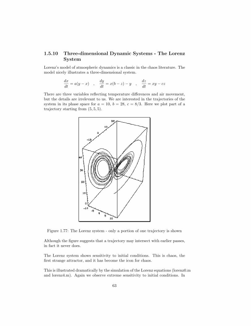
1.5.10 Three-dimensional Dynamic Systems - The LorenzSystem

Lorenz’s model of atmospheric dynamics is a classic in the chaos literature. Themodel nicely illustrates a three-dimensional system.

dx

dt= a(y − x) ,

dy

dt= x(b− z)− y ,

dz

dt= xy − cz

There are three variables reflecting temperature differences and air movement,but the details are irrelevant to us. We are interested in the trajectories of thesystem in its phase space for a = 10, b = 28, c = 8/3. Here we plot part of atrajectory starting from (5, 5, 5).

Figure 1.77: The Lorenz system - only a portion of one trajectory is shown

Although the figure suggests that a trajectory may intersect with earlier passes,in fact it never does.

The Lorenz system shows sensitivity to initial conditions. This is chaos, thefirst strange attractor, and it has become the icon for chaos.

This is illustrated dramatically by the simulation of the Lorenz equations (lorenz0.mand lorenz4.m). Again we observe extreme sensitivity to initial conditions. In

63

fact, this model was the original source of the idea of sensitivity to initial con-ditions!

1.5.11 Beasts in Phase space - Limit Points

There are three kinds of limit points.

Attractors: where the system settles down to.

Repellers: a point the system moves away from.

Saddle points: an attractor from some regions, repeller in others.

Examples

Attractors: we’ve seen many

Repellers: the value 0 in the Logistic Map

Saddle points: the point (0,0) in the Buckling Column

Let us now return to a discussion of the non-linear, damped driven oscillator,which is a real physical system.

1.6 The Nonlinear Damped Driven Oscillator

We have a Newtons second law of the form for a pendulum (we have switchedvariables from x to θ - the angle of a swinging pendulum)

md2θ

dt2+ α

dθ

dt+ β sin θ = γ cos (ωt)

First we investigate the motion of this physical system in phase space. We fixedsome of the parameters

b = 1.0 =β

m=

1

m

√g

`, ` = pendulum length

c = 0.5 =α

m, α = damping parameter

ω = 0.66666666 = driving frequency

We will use as a variable (control) parameter (like λ in the logistic map) theconstant a where a = γ/m. In particular, we will look at

a = 0.90→ periodic motiona = 1.07→ periodic doublinga = 1.15→ chaotic motiona = 1.35→ periodic motiona = 1.45→ periodic doublinga = 1.47→ periodic doublinga = 1.50→ chaotic motion

We run phsp.m to generate the phase space plots shown below:

64

Figure 1.78: a = 0.90 — periodic motion

Figure 1.79: a = 1.07 — periodic doubling

65

Figure 1.80: a = 1.15 — chaotic motion


66



67


The dependence of the system motion on the amplitude is clearly very complexand sensitive to value.

Another way to visualize the behavior of these systems is via Poincare Plots.The Poincare plot is the same as using a stroboscope on the motion. In thiscase we flash the strobe once every cycle of the driving force (frequency = ω).We run phsppoin.m to generate the plots shown below:

68


69


70


71


72


73


74


The Poincare plot in this case is an attractor with an infinite number of points.It is a fractal curve (more about this later) with non-integer dimension. Thesteady state motion of the oscillator at this a and ω is not periodic at all; themotion is chaotic. An attractor of this sort is known as a strange attractor. Itsinfinity of points are arranged in a strange self-similar (fractal) manner.

Finally we can make a bifurcation plot for the driven oscillator, where we plotthe strobe values (from the Poincare plot) versus the driving amplitude.

75

Figure 1.92: Bifurcation Plot

We see the same structure as in the logistic map bifurcation plot. The variousperiodic, period-doubling and chaotic regions are clear. The critical points arealso clear.

Thus, two systems, which really do not resemble each other in any way exceptthat they are both nonlinear systems, exhibits very similar behaviors.

A movie of the calculation is shown in oscpoinbif.mpg.

1.6.1 Zooming in

Let us zoom in on a strange attractor. We consider the Poincare plot for thedriven oscillator when a = 1.50. It looks like the figures below. It is clear thatthere is complex structure in a strange attractor or fractal at all levels. Thedimension of this strange attractor is D = 1.4954....(more later).

76

Figure 1.93: Original Structure

77

Figure 1.94: ZOOM #1 below shows the detail present in the attractor.

78

Figure 1.95: ZOOM #2 below shows further detail present in the attractor.

79

Figure 1.96: ZOOM #3 Pick another place.......

80

Figure 1.97: and zoom again .....

81

Here we are only limited by the resolution of the screen and the accuracy of thecalculation.

The simulations of the chaotic attractor and its Poincare section reveal a hi-erarchical structure that is uncharacteristic of ordinary compact geometricalobjects. The chaotic attractor as represented by the Poincare sections will bediscussed as fractals - mathematical sets of noninteger dimension(strange at-tractors) - later in these notes.

These different magnifications clearly reveal the self-similar structure caused bythe folding and stretching of the phase volume. The stretching and folding pro-cesses lead to a cascade of scales: the attractor consists of an infinite number oflayers. The fine structure resembles the gross structure. This property is calledself-similarity.

Properties

1. The trajectory of a strange attractor cannot repeat.

2. Nearby trajectories diverge exponentially.

3. The attractor is bounded in the phase space.

4. Even though it has an infinite number of different points,the trajectorydoes not fill the phase space.

A strange attractor is a fractal(more later), and its fractal dimension(more later)is less than the dimension of the phase space.

Self-Similarity

An important (defining) property of a fractal is self-similarity, which refers toan infinite nesting of structure on all size scales. Strict self-similarity refers to acharacteristic of a form exhibited when a substructure resembles a superstruc-ture in the same form.

1.7 Appendix

1.7.1 Stability of Fixed Points

An important question is whether a fixed point is stable, that is, they areattractors. To settle this question we start with a point near a fixed point andsee if the result of repeated mapping(iteration) converges to the fixed point. Wewrite xn as

xn = x̄+ δn

where x̄ is a fixed point and δn is (at least initially) small in magnitude. Sub-stituting into the map equation and retaining only terms linear in δn (since δn

82

is small), we find that

xn+1 = x̄+ δn+1 = λ(x̄+ δn)(1− (x̄+ δn))

x̄+ δn+1 = λx̄(1− x̄) + λδn − 2λx̄δn − λ(δn)2

δn+1 = λδn − 2λx̄δn

→ δn+1

δn= λ(1− 2x̄)

where we have used the definition of the fixed point x̄ = λx̄(1−x̄)→ x̄ = 1−1/λand dropped the λ(δn)2 term. If |δn+1| < |δn|, then with repeated mappings thepoint xn = x̄+δn moves closer and closer to x̄ with increasing n and so this fixedpoint is called stable or attracting. On the other hand, if |δn+1| > |δn|, then thepoint moves away from x̄ and the fixed point is called unstable or repelling.

For the logistic mapxn+1 = λxn(1− xn) = F (xn)

and we have (dF

dx

)x=x̄

= λ(1− 2x̄) =δn+1

δn

so that the criterion for stability becomes(dF

dx

)x=x̄

< 1

We note that this result is general for all maps of the form xn+1 = F (xn). Alsonote that (

dF

dx

)x=x̄

is the slope of the mapping function in the neighborhood of the fixed point.

1.7.2 Generating the Lyapunov Exponent Curve

Let us look specifically at a one-dimensional map described by xn+1 = f(xn).We choose the initial difference between the two states to be d0 = ε, and afterone iteration, the difference d1 is

d1 = f(x0 + ε)− f(x0) ≈ ε dfdx

∣∣∣∣x0

where the last result on the right occurs because ε is very small. After n itera-tions, the difference dn between two initially nearby state is given by

dn = fn(x0 + ε)− fn(x0) = εenγ

where we have indicated the nth iterate of the map f(x) by the superscript n.If we divide by ε and take the logarithm of both sides, we have

ln

(fn(x0 + ε)− fn(x0)

ε

)= ln (enγ) = nγ

83

Now, because ε is very small, we have for γ

γ =1

nln

(fn(x0 + ε)− fn(x0)

ε

)=

1

nln

∣∣∣∣dfn(x)

dx

∣∣∣∣x0

The value of fn(x0) is obtained by iterating the function f(x0) n times.

fn(x0) = f(f(.....(f(x0)).....))

We use the derivative chain rule of the nth iterate to obtain

dfn(x)

dx

∣∣∣∣x0

=df(x)

dx

∣∣∣∣xn−1

df(xi)

dx

∣∣∣∣xn−2

.........df(x)

dx

∣∣∣∣x0

Taking the limit as n→∞ we finally obtain

γ = limn→∞

1

n

n−1∑i=0

ln

∣∣∣∣df(x)

dx

∣∣∣∣where the sum arises from the logarithm of a product. We plot (lyapunov.m)theLyapunov exponent as a function of λ, the logistic parameter, below.

Figure 1.98: Lyapunov exponent as a function of λ

Clearly, the Lyapunov exponent is negative whenever the map is! stable andpositive whenever the map is chaotic. The value of γ is zero when bifurcationoccurs because |df/dx| = 1 and the solution becomes unstable. A superstablepoint occurs where df/dx = 0 and this implies that γ = −∞. We can see clearlyfrom the plot that when γ goes above zero, there are windows of stability whereγ goes negative for a while and period orbits occur amid the chaotic behavior.The relatively wide window just above 3.8 is apparent.

84

Chapter 2

Fractals

2.1 Introduction

”Clouds are not spheres, mountains are not cones, coastlines are not cir-cles, and bark is not smooth, nor does lightning travel in a straight line.”(Mandelbrot, 1983)

We now repeat some of the tentative ideas that we mentioned in Chapter 1 andexpand them to a better understanding of the term fractal. Benoit Mandelbrotwas intrigued by the geometry of nature. He was a jack-of-all-trades and wasinterested in all kinds of phenomena. One of the things he investigated wascotton prices.

Economists said that the cotton prices contained an orderly(regular) part anda random part. This implied that in the long term, prices are driven by realforces and that in the short term prices are random.

But the data did not agree!

There were too many large jumps, i.e., the ratio of small price changes to largeprices changes was much smaller than expected. In addition there was a largetail (at the high end) in the distribution of price values.

If prices changed at random, then they would be distributed in what is calledthe normal distribution - the Bell curve. If this were true than the probabilityof price change differing from the mean change by three standard deviationswould be extremely small - the cotton data did not fit a Bell curve!

Economics rules of the road, articles of faith and prejudices imply that small,transient changes have nothing in common with large, long term changes - thatfast fluctuations are random - small scale, short term changes are just noise andthus they are unpredictable. Long term changes, however, are determined by

85

deep macroeconomic forces.

This dichotomy, however, was false. Mandelbrot showed that all changes arebound together - that there is one pattern across all scales. He used computersto show that the cotton prices, which did not obey a normal distribution, pro-duced symmetry from the point of view of scaling - a kind of scale independence.Each particular price change was random and unpredictable, but the sequenceof changes was independent of scale.

Mandelbrot also studied transmission of data - in particular errors in transmis-sion.. Mandelbrot found, contrary to intuition, that you can never find a timeduring which errors were scattered continuously - within any burst of errors,no matter how short, there would always be periods that were completely errorfree.

Mandelbrot found geometric relations between bursts of errors and error-freetransmission periods. The relationship was the same no matter the time scale,namely, the Cantor set, which we will study later. It was a strange scattering ofpoints arranged in clusters - infinitely many but yet infinitely sparse. He showedthat transmission errors are a Cantor set arranged in time.

Mandelbrot also investigated the height of the Nile river. He classified variationsinto

1. Noah effect → discontinuous

2. Joseph effect → persistence

All other researchers had neglected changes of the ”Noah” type. The datashowed that persistence applied over centuries as well as over decades - anotherexample of scale independence.

His research showed that trends in nature are real, but that they can vanish asquickly as they arise.

Discontinuities, bursts of noise, Cantor sets - where does all of this fit intothe classical geometry of lines, planes and circles. Lines, planes and circlesare a powerful abstraction of reality - this kind of abstraction will eliminatecomplexity and prevent any understanding from being developed. As the quoteat the beginning of the chapter states:

clouds 6= spheres

mountains 6= cones

lightning does not travel in straight lines

Mandelbrot proposed that there is a geometry associated with complexity andit implies strange ”shapes” that have a meaning in the real world. Euclidean

86

objects are idealizations and cannot represent the essence of the geometry of anobject in the real world.

Mandelbrot asked - how long is the coastline of Norway? He said, in a sense,that the coastline is infinitely long or that the answer depends on the size of yourruler. Common sense says that a smaller ruler sees finer detail and measuresa longer length - but there must be some limiting value! If the coastline was aEuclidean abstraction, then there would be a limiting value equal to the length.

Thinking about these ideas will lead us to a discussion of dimension. We mightask - what is the dimension of a ball of twine?

1. from a great distance it is a point which says its dimension is 0

2. from closer, it fills spherical space which says that its dimension is 3

3. closer still and the twine is now seen and its dimension is now 1, althoughthe dimension is tangled up making use of 3D space

This tells us, in some way, that the effective dimension is not always equal to 3.

What about ”in between” - non-integer dimension - will nothing be sacred inthis class!

As we will see later, non-integer dimensions are associated with coastlines. Thecoastline will be new kind of curve called a fractal and its length will be infinite!We will learn how to determine the dimension of these fractals - the fractal di-mension will be a way of measuring quantities such as roughness or irregularityin an object - a twisting coastline, despite not being able to measure its length,has a certain degree of roughness. As we will see the fractal dimension willremain constant over different scales.

A simple Euclidean 1D line fills no space at all. We will study a fractal linecalled the Koch curve that has infinite length, but fits into a finite area, com-pletely filling it. It will be seen to be more than a line, but less than a planeand cannot be represented by Euclidean geometry. Its dimension will be greaterthan 1 but less than 2 (actually 1.2618).

Smooth curves are 1D objects whose length can be precisely defined betweentwo points. A fractal curve has an infinite variety of detail at each point alongthe curve implying more and more detail as we zoom in, which implies that thelength will be infinite.

Suddenly fractals were everywhere. They were found to be hidden in all kindsofdata.

The property that one has infinite detail at each point and the detail looks like

87

the original is called self-similarity. Self-similarity is symmetry across scale orrecursion or patterns within patterns.

At first sight, the idea of consistency on new scales seems to provide less in-formation. This seems so because it goes against the tradition of reduction-ism(building blocks). The power of self-similarity begins at much greater levelsof complexity. It will be a matter of looking at the whole, rather than the parts.

We now turns to a detailed study of fractals. At that point we will have devel-oped all the necessary tools to make and understand a science of chaos.

2.2 The Nature and Properties of Fractals

Fractals are mathematical sets of point with fractional dimension.

Fractals are not simple curves in Euclidean space. A Euclidean object hasintegral dimension equal to the dimension of the space the object is being drawnin. In addition, if a Euclidean line connects 2 points in 3-dimensions and alsostays within a finite volume, then the length of the line is finite.

A fractal is a line that can stay within a finite volume, but still have an infinitelength. This implies that it has a complex structure at all levels of magnification.In comparison, a Euclidean line will eventually look like a straight line at somemagnification level.

To describe this property of a fractal, we need to generalize the usual conceptof dimension.

The dimensionality D of a space is usually defined as the number of coordinatesneeded to determine a unique point in that space. When defined in this way,the only allowed values for D are the non-negative integers 0, 1, 2, 3, ... There areseveral ways that the concept of dimension can be redefined so that it still takeson non-negative integer values when considering the systems described above,but can also take on non-negative real number values.

We will adopt a simplified version of the Hausdorff dimension called the boxcounting or capacity dimension. In the box-counting scheme, the dimensionof an object is determined by asking how many boxes are needed to cover theobject. Here the appropriate boxes for coverage are lines, squares, cubes, etc.The size of the boxes is repeatedly decreased and the dimension of the object isdetermined by how the number of covering boxes scales with the length of theside of the box.

fractal: An irregular shape with self-similarity. It has infinite detail, andcannot be differentiated. Wherever chaos, turbulence, and disorder arefound, fractal geometry is at play.

88

fractal dimension: A measure of a geometric object that can take onfractional values. At first used as a synonym to Hausdorff dimension,fractal dimension is currently used as a more general term for a measureof how fast length, area, or volume increases with decrease in scale.

2.3 The Concept of Dimension

So far we have used the concept of dimension in two senses:

1. The three dimensions of Euclidean space (D = 1, 2, 3)

2. The number of variables in a dynamic system

Fractals, which are irregular geometric objects, require a third meaning.

In one dimension, we consider a line of length `. We need

1 box(a line) of length `

2 boxes of length `/2

...................

2m boxes of length `/2m

...................

If we define δm = length of the mth box, then

δm =`

2m

Thus, the number of boxes N(δm) scales (grows) as

N(δm) =`

δm

In two dimensions, we consider a square of side `. We need

1 box(a square now) of area `2

4 boxes of area (`/2)2

...................

2m boxes of area (`/2m)2

...................

89

Thus, the number of boxes N(δm) scales (grows) as

N(δm) =

(`

δm

)2

Generalizing to D integer dimensions, we have

N(δm) =

(`

δm

)DNow to do some algebra (the details of the algebra are not important, but thefinal result is important). We have

log (N(δm)) = log

(`

δm

)D= D log

(`

δm

)= D(log (`)− log δm)

→ D =log (N(δm))

log (`)− log (δm)

We then define the dimension D by

D = limm→∞

log (N(δm))

log (`) + log(

1δm

)As m→∞, log (`) becomes negligible compared to other terms and we have

D = limm→∞

log (N(δm))

log(

1δm

) = limε→0

log (N(ε))

log (1/ε)

where N(ε) = the number p−dimensional cubes of side ε needed to completelycover the set.

This is the Hausdorff or fractal dimension D of a set of points in a p−dimensionalspace.

Wow! That was a very mathematical and tedious derivation. We can makeclear the meaning of the result by some examples.

Examples:

(1) A single point: only one cube is required. This means that

N(ε) = 1→ logN(ε) = 0→ D = 0

as expected.

90

(2) A line of length `: The number of cubes of side ε required = number ofline segments of length ε . Therefore

N(ε) =`

ε

and

D = limε→0

log(`ε

)log(

1ε

)= limε→0

log(

1ε

)+ log (`)

log(

1ε

)= limε→0

(1 +

log (`)

log(

1ε

)) = 1

as expected.

(3) a square of area `2: The number of cubes of side ε required = numberof squares of side ε. Therefore

N(ε) =`2

ε2

and

D = limε→0

log(`2

ε2

)log(

1ε

)= limε→0

2 log(

1ε

)+ log (`2)

log(

1ε

)= limε→0

(2 + 2

log (`)

log(

1ε

)) = 2

as expected.

So this definition of dimension works for Euclidean objects and clearly makessense.

An alternative way to think about it. It is always good to look at a new conceptin several ways!

2.3.1 The Hausdorff Dimension

If we take an object residing in Euclidean dimension D and reduce its linearsize by 1/r in each spatial direction, its measure (length, area, or volume) wouldincrease to N = rD times the original. This is pictured in the figure below.

91

Figure 2.1: size reductions

We consider N = rD, take the log of both sides and get

log (N) = D log (r)

If we solve for D we get

D =log (N)

log (r)

The point of this exercise: Examined this way, D need not be an integer, as itis in Euclidean geometry. It could be a fraction, as it is in fractal geometry. Thisgeneralized treatment of dimension is named after the German mathematician,Felix Hausdorff. It has proved useful for describing natural objects and forevaluating trajectories of dynamic systems.

2.3.2 The length of a coastline

Mandelbrot began his treatise on fractal geometry by considering the question:How long is the coast of Britain?

The coastline is irregular, so a measure with a straight ruler, as in the nextfigure, provides an estimate. The estimated length L, equals the length of the

92

ruler, s, multiplied by the N, the number of such rulers needed to cover themeasured object. In the figure below we measure a part of the coastline twice,the ruler(unit of measurement) on the right is half that used on the left.

Figure 2.2: measuring coastline length using rulers of varying lengths

But the estimate on the right is longer. If the scale on the left is one, we havesix units, but halving the unit gives us 15 rulers (L = 7.5), not 12 (L = 6). Ifwe halved the scale again, we would get a similar result, a longer estimate of L.In general, as the ruler gets diminishingly small, the length gets infinitely large.

The concept of length, begins to make little sense.

2.3.3 The Cantor Set

Consider the figure below.

93

Figure 2.3: construction of the Cantor set

In the above diagram, points in the interval (0, 1) are tracked for 4 iterations.On the 1st iteration, the middle third of the points leave the interval (0, 1). Themiddle thirds of the two in segments leave the interval and so on. The bottomrow(after infinite iterations) is the Cantor set.

The Cantor set has some stunning properties. For one thing, in the infinite limitit has zero measure (it is the empty line). But the set is far from empty, in fact,it has an uncountable number of points.

To cover the set at step K we need

N(K) = 2K cubes of side ε =

(1

3

)KTherefore,

D = limK→∞

log (2K)

log((

13

)K) = limK→∞

K log (2)

K log (3)=

log (2)

log (3)= 0.631

The dimension of the Cantor set is not an integer !

94

2.3.4 The Koch Snowflake

The Koch curve is constructed by recursion as exhibited in the figures below.At each step the middle-third of each segment is replaced with a ”V” shapedbulge. This curve turns out to have infinite length, while enclosing (togetherwith its natural base: the original line segment) a finite area. Demo the KochSnowflake.

We begin with a straight line of length 1, called the initiator. We then removethe middle third of the line, and replace it with two lines that each have thesame length (1/3) as the remaining lines on each side. This new form is calledthe generator, because it specifies a rule that is used to generate a new form.

The rule says to take each line and replace it with four lines, each one-third thelength of the original.

Figure 2.4: Original Line

Figure 2.5: Step #1

95

Figure 2.6: Step #2

Figure 2.7: Step #3

Figure 2.8: Step #4

96

Figure 2.9: Step #5

The dimension of the Koch snowflake is given by

D = limn→∞

log (4n)

log((

13

)n) = limn→∞

n log (4)

n log (3)=

log (4)

log (3)= 1.26....

We get a dimension between 1 and 2. Clearly, the final length of the fractal line

limn→∞

(4

3

)n→∞

is infinite even though it stays within a finite area of the 2-dimensional Euclideanplane.

2.3.5 Sierpinski Triangle

The figures below illustrate the construction of the Sierpinski triangle by itera-tion:

97

Figure 2.10: Starting Configuration

Figure 2.11: Step #1

98

Figure 2.12: Several steps later

Calculating the dimension.

D =log (N)

log (r)=

log (3)

log (2)= 1.585....

Again we get a number between 1 and 2.

99

Figure 2.13: Many iterations

2.3.6 IFS Fractals

One method of generating fractals is to choose dilation(rescaling) and transla-tion transformations at random. Say, for example, that we adopt the iterativedilation/translation map given by:(

xn+1

yn+1

)=

(a bc d

)(xnyn

)+

(ef

)xn+1 = axn + byn + e

yn+1 = cxn + dyn + f

where the [a, b, c, d] dilation matrix and the [e, f ] translation vector are chosenrandomly. A fern can be generated using appropriate matrix choices:run fern.m.

100

Figure 2.14: [a, b, c, d, e, f ] values with probability of choice

Figure 2.15: A Fractal Fern

101

Demo Fern I and Fern II, sierpinski.m, barnsley.m, Sierpinski Arrowhead, Beech-Branch, Bush, ElmBranch, Plant, Tree 1, Tree 2, Tree 3 and Koch Snowflake.

2.4 Fractal Dimension Program

We now illustrate a program that carries out the box dimension calculations oncomplex fractal structures. The idea of covering a fractal with boxes is shownbelow.

Figure 2.16: Koch curve covered by boxes of size r

The program simply chooses a ”box” size, covers the fractal and counts thenumber of boxes. It then reduces the box size and repeats until the box issmall. At that point it can recognize the limit of plot logN(r) versus log r anddetermine the slope which corresponds to the dimension.

If we apply the program to the Koch snowflake which looks like

102

Figure 2.17: Koch snowflake curve

we get the result

reality:fdc_mac boccio$ ./fdc -i snowflake.tga -b1 200 -b2 8 -n 1 -bf 1.2 -p

FDC - Fractal Dimension Calculator

Initialising GLUT

Creating windows

Creating menus (Right mouse button)

Reading file "snowflake.tga"

Image dimensions: 1188 x 695 x 24

Creating screen version

Full screen size: 2560 x 1440

Display size: 1188 x 695

Scale factor: 1

Processing starting

Box size: 200 [ 1], Total count = 15

















Processing finished

Estimated fractal dimension: 1.211

103

Figure 2.18: log(N)/log(r) plot

Even more dramatic we apply the program to a fractal tree(created on thecomputer) as shown below

104

Figure 2.19: fractal tree

and get the result

reality:fdc_mac boccio$ ./fdc -i tree.tga -b1 200 -b2 8 -n 1 -bf 1.2 -p


Initialising GLUT

Creating windows


Reading file "tree.tga"





Scale factor: 2

Processing starting











105








Processing finished



What about a picture of a real tree? I found a picture of a real tree and put itinto the program

106

Figure 2.21: real tree

and the result is

reality:fdc_mac boccio$ ./fdc -i tree-569.tga -b1 200 -b2 8 -n 1 -bf 1.2 -p


Initialising GLUT

Creating windows


Reading file "tree-569.tga"





Scale factor: 1

Processing starting












107







Processing finished


The log(N)/log(r) graph looks like:


2.5 Complex Maps

To see the self similar nature of fractals even more dramatically we now study2-dimensional complex maps. In particular we look at the Mandelbrot fractalboundary and the cube roots of 1 via Newtons rule(called the Newton attractor).

108

2.5.1 Mandelbrot Sets

The key mapping is a quadratic map given by:

zn+1 = z2n + c

where the zn are complex numbers and c is a complex parameter. It turns outthat if |zn| > 2 further iteration of this quadratic map is unbounded, i.e., fordifferent values of c, the trajectories either stay near the origin or escape toinfinity. When calculations are done we stop the iteration when this conditionis satisfied.

When investigating these maps, one iterates the equation as follows:

(a) start with a complex value for c inside a rectangular boundary

(b) iterate the equation until either

(1) |zn| > 2

or

(2) a preset number of iterations is exceeded

In case (1) color the starting point (c) in red. In case (2) leave the point (c)black. The boundary between the two regions is the Mandelbrot fractal as shownbelow.

Figure 2.23: The Mandelbrot Fractal Boundary

109

Alternately, in case (1) color the starting point (c) by the number of iterationsit took to escape. In case (2) leave the point (c) a single color (say dark blue).

The boundary between the two regions is still the Mandelbrot fractal as shownbelow, but a wide variety of spectacular images can be generated by a cleverchoice of colormap.

Figure 2.24: The Mandelbrot Fractal Boundary - Different Coloring Scheme

or choosing a different colormap(no change in information) we get

Figure 2.25: The Mandelbrot Fractal Boundary - Different Coloring Scheme

110

Run Complex Explorer for colormaps and zooming.

If we zoom far enough we will see the entire repeating itself as all fractals dosince they are self-similar.

2.6 So what is a fractal?

It is an irregular geometric object with an infinite nesting of structures at allscales.

2.6.1 Why do we care about fractals?

natural objects are fractals

chaotic trajectories (strange attractors) are fractals

assessing the fractal properties of an observed time series is informative

complex systems that self-organize will have self-similar or fractal behaviorat all scales

complexity: While, chaos is the study of how simple systems can gen-erate complicated behavior, complexity is the study of how complicatedsystems can generate simple behavior. An example of complexity is thesynchronization of biological systems ranging from fireflies to neurons.

complex system: Spatially and/or temporally extended nonlinear sys-tems characterized by collective properties associated with the system asa whole–and that are different from the characteristic behaviors of theconstituent parts.

2.7 Final Example - The Cube Roots of 1

Another interesting map is called the Newton attractor. In this case one startswith an equation like

z3 − 1 = 0

which is to be solved via the classical Newton iteration method for finding zeroes:

z3 − 1 = 0 = f(z)

zn+1 = zn −f(zn)

df(zn)/dz= zn −

z3n − 1

3z2n

=2

3zn +

1

z2n

In this case one starts with some initial complex point z0. One then iteratesuntil the answer stops changing (converges to one of the three complex rootsof 1). One might assume that the plane will divide up into three pie shapedwedges such that all starting points in a given wedge are closest to one of the

111

three roots(in its basin) and eventually end up at that closest root (the basinattractor). In fact, this does not happen. The boundaries of the wedges are”nibbled” at by interlaced basins of attraction for all the roots producing acomplex fractal boundary as shown below.

Figure 2.26: The Newton Attractor Map

112

If we zoom in on the boundary we see the complex self-similar structure of thefractal strange attractor making up the boundaries between the basins as shownbelow.


113

Further zooming in produces shows the self-similar structure of the fractalboundary.


114

notes for chaos and fractals - john boccio website

Documents