note of use of the contact
TRANSCRIPT

Code_Aster Versiondefault
Titre : Notice d'utilisation du contact Date : 31/07/2018 Page : 1/39Responsable : KUDAWOO Ayaovi-Dzifa Clé : U2.04.04 Révision :
22dbb3cb313f
Note of use of the contact in Code_hasster
Summary:
This document describes the approach to be followed for the taking into account of conditions of contact-frictionin the nonlinear studies. One is interested in surface contact between solids deformable or a deformable solidand a rigid solid. Initially, one points out what means to take into account contact-friction in mechanics of thestructures, then one traces the broad outlines of a problem of contact in Code_hasster : pairing and resolution.
The definition of the contact is carried out with the order DEFI_CONTACT while the resolution is done with theorders STAT_NON_LINE or DYNA_NON_LINE. One formulates recommendations for the parameterization ofpairing and the choice of the methods of resolution in these operators.
Finally various methodologies are evoked (contact with a rigid surface, to recover a contact pressure inpostprocessing, great deformations and contact, movements of rigid bodies blocked by the contact,…). Theymake it possible to overcome the difficulties frequently encountered in the studies. In this section, are alsoapproached alternative modelings of the phenomenon of contact-friction by elements of joints or elementsdiscrete (through the law of behavior).
Warning : The translation process used on this website is a "Machine Translation". It may be imprecise and inaccurate in whole or in partand is provided as a convenience.Copyright 2021 EDF R&D - Licensed under the terms of the GNU FDL (http://www.gnu.org/copyleft/fdl.html)
Code_Aster Versiondefault
Titre : Notice d'utilisation du contact Date : 31/07/2018 Page : 2/39Responsable : KUDAWOO Ayaovi-Dzifa Clé : U2.04.04 Révision :
22dbb3cb313f
Contents
1 Introduction ........................................................................................................................................... 4
1.1 Object of this document ................................................................................................................. 4
1.2 A question of vocabulary ................................................................................................................ 4
1.3 Alternative modelings of contact-friction ......................................................................................... 6
2 Pairing .................................................................................................................................................. 6
2.1 Concept of zones and surfaces of contact ..................................................................................... 6
2.2 Choices of surfaces main and slaves ............................................................................................. 7
2.2.1 Case where a surface must be selected like mistress (GROUP_MA_MAIT) ........................ 8
2.2.2 Case where a surface must be selected like slave (GROUP_MA_ESCL) ............................ 8
2.2.3 Case general ........................................................................................................................ 8
2.2.4 Orientation of the normals ..................................................................................................... 9
2.2.5 Smoothness and degree of grid of curved surfaces .............................................................. 9
2.2.6 Sharp angles ....................................................................................................................... 10
2.2.7 Quality of the grid ................................................................................................................ 10
2.3 Control of pairing .......................................................................................................................... 10
2.3.1 Choice of the type of pairing ............................................................................................... 10
2.3.2 Smoothing of the normals ................................................................................................... 11
2.3.3 Choice of the normals: case formulation other than method LAKE ..................................... 11
2.3.4 Exclusion of nodes slaves of pairing: case formulation other than method LAKE ............... 11
2.4 To understand geometrical non-linearity ....................................................................................... 11
2.4.1 Assumption of small slips .................................................................................................... 11
2.4.2 Case general ...................................................................................................................... 12
2.4.2.1 Buckle of point fixes (ALGO_RESO_GEOM=' POINT_FIXE') ................................ 12
2.4.2.2 Algorithm of generalized Newton (ALGO_RESO_GEOM=' NEWTON') .................. 12
2.4.3 Convergence of the loop of geometry ................................................................................. 13
2.4.3.1 Linearization of the normal ..................................................................................... 13
2.4.3.2 Geometrical convergence criteria ........................................................................... 13
3 Resolution ........................................................................................................................................... 15
3.1 Outline general of the algorithm of resolution ............................................................................... 15
3.1.1 Definition and general remarks ........................................................................................... 15
3.1.2 Discrete formulation ............................................................................................................ 15
3.1.3 Continuous formulation: case ALGO_CONT=' STANDARD'/‘PENALIZATION‘ ................... 17
3.1.4 Continuous formulation: case ALGO_CONT='LAKE‘ .......................................................... 19
3.1.5 Continuous formulation: treatment of the incompatibilities. ................................................. 19
3.2 Resolution of a problem with contact alone .................................................................................. 21
3.2.1 Dualisation in discrete formulation (FORMULATION=' DISCRETE') .................................. 21
3.2.1.1 Principle .................................................................................................................. 21
Warning : The translation process used on this website is a "Machine Translation". It may be imprecise and inaccurate in whole or in partand is provided as a convenience.Copyright 2021 EDF R&D - Licensed under the terms of the GNU FDL (http://www.gnu.org/copyleft/fdl.html)

Code_Aster Versiondefault
Titre : Notice d'utilisation du contact Date : 31/07/2018 Page : 3/39Responsable : KUDAWOO Ayaovi-Dzifa Clé : U2.04.04 Révision :
22dbb3cb313f
3.2.1.2 Method ‘FORCED’ .................................................................................................. 21
3.2.1.3 Method ‘GCP’ ......................................................................................................... 22
3.2.2 Penalization in discrete formulation: algorithm ‘PENALIZATION’ ........................................ 22
3.2.3 Formulation ‘CONTINUOUS’: council on the solveurs and parallelism ............................... 23
3.2.4 Other advices in parallelism ................................................................................................ 24
3.3 Resolution of a problem with friction ............................................................................................ 24
3.3.1 Treatment of the non-linearity of threshold .......................................................................... 24
3.3.2 Discrete formulation: penalization of friction (algorithm ‘PENALIZATION‘) ......................... 24
3.3.3 Formulation ‘CONTINUOUS‘: STANDARD/PENALISATION. ............................................. 25
3.4 Summary for the choice of the methods of resolution .................................................................. 25
3.4.1 For contact-friction .............................................................................................................. 25
3.4.2 For the linear system .......................................................................................................... 26
4 Methodologies .................................................................................................................................... 26
4.1 What to make when a calculation of contact does not converge or doesn't converge towards the
good solution? .............................................................................................................................. 26
4.2 Postprocessing of CONT_NOEU ................................................................................................. 29
4.3 To recover the contact pressure ................................................................................................... 30
4.3.1 presentation of CALC_PRESSION ..................................................................................... 30
4.3.2 Case of Fcontinuous ormulation ......................................................................................... 30
4.3.3 Discrete formulation ............................................................................................................ 31
4.4 Movements of rigid bodies blocked by the contact ....................................................................... 31
4.4.1 Continuous formulation ....................................................................................................... 31
4.4.2 Discrete formulation ............................................................................................................ 32
4.5 Great deformations, great displacements and contact ................................................................. 33
4.5.1 To uncouple non-linearities ................................................................................................. 33
4.5.2 To parameterize the algorithm of Newton well .................................................................... 33
4.5.3 Resolution of a quasi-static problem in slow dynamics ....................................................... 34
4.6 Rigid surface and contact ............................................................................................................. 34
4.7 Redundancy between conditions of contact-friction and boundary conditions (symmetry):
methods other than LAKE ............................................................................................................ 35
4.8 To measure the interpenetration without solving the contact: methods other than LAKE ............. 36
4.9 To display the results of a calculation of contact .......................................................................... 36
4.10 Specific contact with discrete elements (springs) ....................................................................... 37
4.11 Elements of joints (hydro) mechanical with contact and friction ................................................. 37
4.12 Use of the adaptive methods ..................................................................................................... 37
5 Bibliography ........................................................................................................................................ 39
Warning : The translation process used on this website is a "Machine Translation". It may be imprecise and inaccurate in whole or in partand is provided as a convenience.Copyright 2021 EDF R&D - Licensed under the terms of the GNU FDL (http://www.gnu.org/copyleft/fdl.html)

Code_Aster Versiondefault
Titre : Notice d'utilisation du contact Date : 31/07/2018 Page : 4/39Responsable : KUDAWOO Ayaovi-Dzifa Clé : U2.04.04 Révision :
22dbb3cb313f
1 Introduction
1.1 Object of this document
To say that two solid bodies put in contact do not interpenetrate but that on the contrary a reciprocaleffort is exerted one on the other and that this effort disappears when the bodies are not touched anymore, concerns the good sense. It is the briefest definition which one can make of the problem of“contact”: however to enforce these conditions in a computer code of the structures like Code_Asterrequest much for efforts.
To solve the problem of contact, it is finally to impose a boundary condition inequalities on certaindegrees of freedom of displacement (negative or null game) and to find an unknown factor additionalwho is reciprocal effort being exerted between the two bodies.
The difficulty comes from the strong non-linearity induced by this “pseudo-condition in extreme cases”.Indeed, the condition to be imposed on displacements (to prevent any interpenetration) depends iteven on displacements (which will determine in which point surfaces make contact).
Non-linearity due to the taking into account of contact is separate in Code_Aster in two points:• non-linearity of contact (- friction): it rises from the conditions of contact (- friction) which
are not differentiable. To solve the problem, one has two large families of resolution whichare: the formulation DISCRETE and the formulation CONTINUOUS. The first family isadapted to the problems with low number of unknown factors of contact and allows timescomputings fast while second is adapted to the problems requiring the taking into accountof other non-linearities mechanics with contact-friction (plasticity and greattransformations).
• geometrical non-linearity: it rises from the great relative slips likely to occur betweensurfaces in contact (ignorance a priori effective final surfaces of contact). One calls hereon an algorithm of fixed point or Newton coupled to a geometrical research.
In Code_Aster, in the presence of contact, the user must has minimum to identify potential surfaces ofcontact. The technique of resolution rests then on two fundamental stages:
• Phase of pairing: it makes it possible to treat geometrical non-linearity as a succession ofproblems in small slips (where the problem is geometrically linear). The technique todetermine effective surfaces of contact and the advices of parameter setting of this phaseare given to the section 2.
• Phase of resolution: it makes it possible to solve the problem of optimization underconstraints related to the non-linearity of contact and possibly of friction. The variousalgorithms of optimization available are presented in the section 3. One gives a advanceto it to choose an algorithm adapted to his case of study.
It is essential to have understood that contact-friction is a non-linearity except for whole as well as non-linearities materials (law of nonlinear behavior) and kinematics (great displacements, great rotations).She thus asks at the same time to know the bases of the theory of the contact and to understand thetreatment of this one in Code_Aster in order to make the good choices of modeling (grid and setting indata).
This document is there to assist the user in these choices.
1.2 A question of vocabulary
In order to facilitate the reading, one gives here some of the terms abundantly used in this document.
When one speaks about contact mechanics, one uses two characteristic sizes:• often noted game g or d. It characterizes the distance signed between two surfaces of
contact;
Warning : The translation process used on this website is a "Machine Translation". It may be imprecise and inaccurate in whole or in partand is provided as a convenience.Copyright 2021 EDF R&D - Licensed under the terms of the GNU FDL (http://www.gnu.org/copyleft/fdl.html)
Code_Aster Versiondefault
Titre : Notice d'utilisation du contact Date : 31/07/2018 Page : 5/39Responsable : KUDAWOO Ayaovi-Dzifa Clé : U2.04.04 Révision :
22dbb3cb313f
• density the effort of contact p. It is the reciprocal effort exerted by a solid on the other whenthe game is closed (null). It is carried by the normal on the surfaces of contact. One will alsowrongly use the term of contact pressure.
• Zone Master & slave: It is about a border of solid on which one will impose the conditions ofcontact-friction. The contact is defined by “couples solids”. In each couples, the master-slaverole is crucial for the good progress of a calculation.
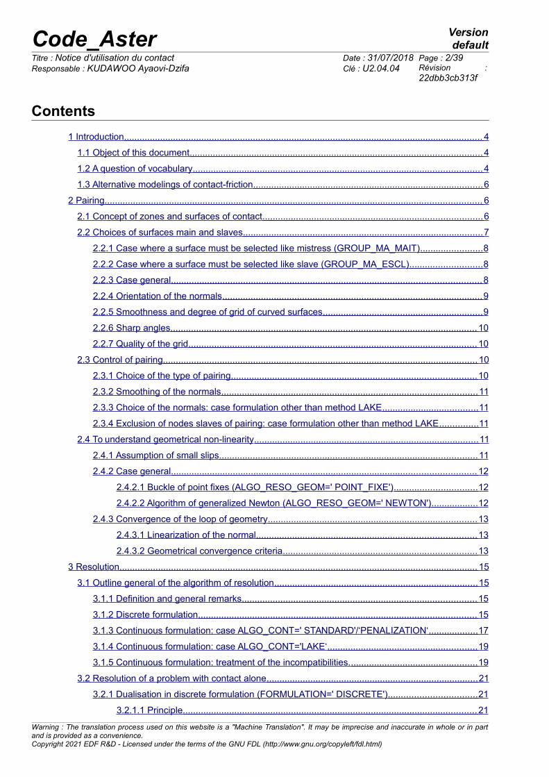
• Incompatible grids: They is the cases where mesh Master does not coincide with the meshslave. These cases are extremely difficult to manage. The best method for these cases aremethod MORTAR known as LAKE usable in formulation only continues. One will also speakthe strong ones or weak incompatibilities about grids. There are not a rigorous criterion todeclare strong or a weak incompatibility. One lets to art engineer decide it according to thecase to treat. One illustrates nevertheless in the figure below an example of strong and weakincompatibility.
Figure 1.2-1: Examples of incompatibilities of grid
• States of contact: it is the couple (game-pressure) characterizing an element of contact. Thereare 2 states of possible contact: contact (null game, nonworthless pressure) and separation(game not no worthless pressure). Two situations being exclusive. Each state can havealternatives: shaving contact (game almost no one, nonzero but low pressure), frank contact(null game and contact pressure high), shaving separation (opposite shaving contact), frankseparation (opposite of frank contact)
• Cycling: it is about a frequent case of nonconvergence in calculations of contact. The situationof cycling it is when a point of contact or a mesh of contact has difficulty stabilizing its statute(contact/not contact, adherence/slip, slip/before/back slip).
• Laws of contact of Hertz-Signorini-Moreau: like any law of behavior, the interfaceS betweensolids have their clean formalismS mathematicsS. The laws of contact derive from a formalismof nonregular mechanics (just like the problems of breaking process or of cohesion forexample): absence of a differentiable energy from which one can write a relation force-displacement easily.
• LAKE or Mortar LAKE: Room Average Contact, it is a method adapted to the incompatiblegrids.
• Oscillating contact pressures: in the case of incompatible grids, it can happen that contactpressures present an oscillating character. One notices it thanks to a substantial dispersion ofthe values of contact pressure.
One describes in detail Cbe sizes in Doc. of reference [R5.03.50].
In the presence of friction, one introduces in addition:• direction of slip t• density the effort of friction , carried by − t⃗ .
In Code_Aster, one uses a criterion of friction of Coulomb, the conditions of friction are described in[R5.03.50].
Warning : The translation process used on this website is a "Machine Translation". It may be imprecise and inaccurate in whole or in partand is provided as a convenience.Copyright 2021 EDF R&D - Licensed under the terms of the GNU FDL (http://www.gnu.org/copyleft/fdl.html)
Weak incompatibility
Weak incompatibility
Strong incompatibility
Strong incompatibilities

Code_Aster Versiondefault
Titre : Notice d'utilisation du contact Date : 31/07/2018 Page : 6/39Responsable : KUDAWOO Ayaovi-Dzifa Clé : U2.04.04 Révision :
22dbb3cb313f
1.3 Alternative modelings of contact-friction
If the manner of treating the phenomenon of contact-friction described in introduction and in theessence of this document is most widespread, it is not only. Code_Aster thus propose two alternativemodelings of the mechanical interactions:
• elements of joints (hydro) mechanical (modelings *_JOINT*) for the representation of theopening of a crack under the pressure of a fluid and friction enters the walls of the closedcrack
• discrete elements of shock (modelings *_DIS_T*) for the representation of a specificcontact by springs with possible taking into account of friction
These two other modelings are based both on finite elements and thus on specific laws of behavior(JOINT_MECA_FROT for the elements of joints and DIS_CHOC for the discrete elements).
More precise details on these elements are provided to the §4.10 and §4.11.
To finish, it will be noted that it is possible to model contact on the edges of a crack represented withmethod X-FEM. One will refer to the note [U2.05.02] for more information.
2 Pairing
2.1 Concept of zones and surfaces of contact
It is always to the user to define surfaces potential of contact: there does not exist in Code_Aster ofautomatic mechanism of detection of the possible interpenetrations in a structure.
The user thus provides in the command file a list of couples of surfaces of contact. Each couplecontains one surface said “main” and one surface said “slave”. One calls “ zone of contact “such acouple.
Case pairing MAIT_ESCL :The conditions of contact will be imposed zone by zone. To enforce the contact consists with toprevent the nodes slaves from penetrating inside surfaces Masters (on the other hand the reverseis possible).On the example below (cf. Figure 2.1-1), the studied structure consists of three solids, one definedthree potential zones of contact symbolized by the red ellipses. As their name indicates it these zonesof contact determine parts of the structure where bodies are likely to make contact. That means thatone enforced the conditions of contact-friction there, the effective activation of dependent contact infine imposed loading.
There is no restriction on the number of zones of contact. The zones must however be separate, i.e.the intersection of two distinct zones must be empty1. In addition, within a zone, surfaces Masters andslaves of the same zone must also have a worthless intersection: if it is not the case, calculation isstopped. When a node is obligatorily common to surfaces Masters and slaves, because of a constraintof grid for example, to refer to the §2.3.4 for a solution. If a continuous formulation is used (cf. 3.1.3),surfaces slaves must imperatively be two to two disjoined.One should not hesitate to describe broad zones of contact to avoid any interpenetration. It is thenumber of nodes of the surface slave which is determining in the cost of calculation. Surface Mastercan, it, being as large as it is wished.
It is imperative that the nodes of surfaces of contact (Masters and slaves) carry all of thedegrees of freedom of displacement (DX, DY and possibly DZ), i.e. they belong with meshs of themodel. An error message stops the user if it is not the case. One will refer to the §4.6 for the modelingof a contact with a rigid surface.
1 More precisely it is the intersection of surfaces slaves which must be emptyWarning : The translation process used on this website is a "Machine Translation". It may be imprecise and inaccurate in whole or in partand is provided as a convenience.Copyright 2021 EDF R&D - Licensed under the terms of the GNU FDL (http://www.gnu.org/copyleft/fdl.html)

Code_Aster Versiondefault
Titre : Notice d'utilisation du contact Date : 31/07/2018 Page : 7/39Responsable : KUDAWOO Ayaovi-Dzifa Clé : U2.04.04 Révision :
22dbb3cb313f
Figure 2.1-1: Definition of three zones of contact
Case pairing MORTAR :When one has calculations with incompatible grids and that one needs to estimate the states of contactprecisely, one recommends to use the method MORTAR LAKE . This method calculation makes itpossible to do calculations of contact on intersected couples SURFACE ESCL on SURFACE MAITcontrary to the method of pairing MAIT_ESCL who associates NODE S with SEGMENT S.
With this intention, there is a necessary stage which consists in pretreating the grid before the use ofDEFI_CONTACT : CREA_MAILLAGE/DECOUPE_LAC . This stage prepares the surface of contactslave for an integration of the terms of contact of the type MORTAR on the intersected meshs.
This method owing to the fact that it uses a surface-to-surface approach observes best the conditionsof interpenetrations Master/slave and main slave/. As for the method MAIT_ESCL, the user mustdefine couple by couple the potential zones of contact. There is no restriction on the number of zonesof contact.
Dthem distinct zones can have common nodes but not of common meshs because the condition ofcontact is imposed on the meshs. In addition, within a zone, surfaces Masters and slaves of the samezone must also have a worthless intersection. The kinematics quantities of contact for methodMORTAR are geometrical fields by element.
2.2 Choices of surfaces main and slaves
As one has just said it, each zone of contact consists of a surface Master and a surface slave. In theactual position, one cannot make auto--contact in Code_Aster (except in the rare cases where one canpredict the future zone of contact and thus define a slave and a Master).
The need to differentiate two surfaces comes from the technique adopted in calculation from the game.This calculation is carried out in a phase that one names pairing.
In the case of pairing MAIT_ESCL , LE game is defined in any point of surface slave (for the discretemethods it is the nodes, for the continuous methods of the points of integration) as the minimaldistance to surface Master. This dissymmetry implies a choice which can a priori to prove to be difficult(how to decide?). The points which must prevail in this choice are given in the following paragraphs.In the case of pairing MORTAR, LE game is defined by patch intersected surface slave-surface Master. One informs these surfaces in the operator DEFI_CONTACT under the keyword factor ZONE.
Warning : The translation process used on this website is a "Machine Translation". It may be imprecise and inaccurate in whole or in partand is provided as a convenience.Copyright 2021 EDF R&D - Licensed under the terms of the GNU FDL (http://www.gnu.org/copyleft/fdl.html)

Code_Aster Versiondefault
Titre : Notice d'utilisation du contact Date : 31/07/2018 Page : 8/39Responsable : KUDAWOO Ayaovi-Dzifa Clé : U2.04.04 Révision :
22dbb3cb313f
2.2.1 Case where a surface must be selected like mistress (GROUP_MA_MAIT)
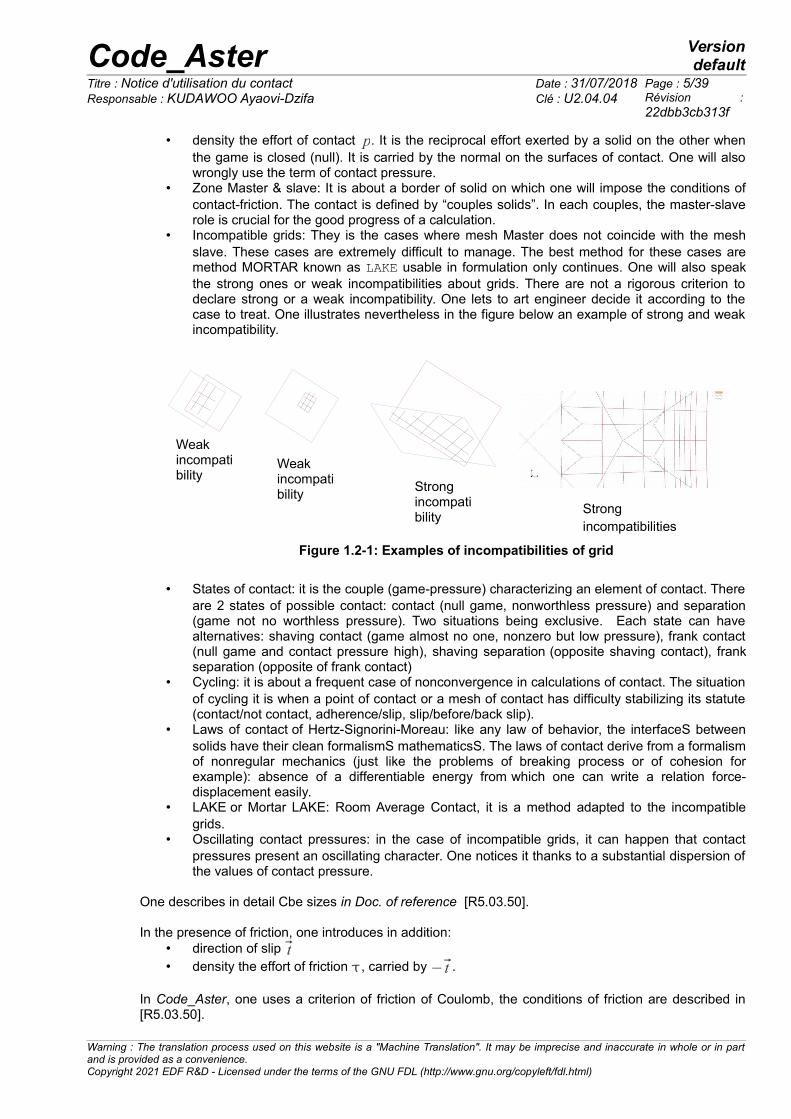
When one of these conditions is joined together:• one of two surfaces east rigid (A);• one of two surfaces recover the other (b);• one of two surfaces has an apparent rigidity large in front of the other (“apparent” with the
direction where one does not speak about the Young moduli but about the stiffnesses inN.m−1) (c);
• one of two surfaces is with a grid much more coarsely that the other (d);
then this one must be selected like surface Master.
2.2.2 Case where a surface must be selected like slave (GROUP_MA_ESCL)
When one of these conditions is joined together: • one of two surfaces east curve (A);• one of two surfaces is more small that the other (b);• one of two surfaces has an apparent rigidity small in front of the other (c);• one of two surfaces is with a grid much more finely that the other (d);
then this one must be selected like surface slave.
2.2.3 Case general
At the time of the study of complex structures, it happens that the rules given to the §2.2.1 and §2.2.2are difficult to apply. For example when a solid is almost rigid (with respect to the other solid) and thatit is curved, the rule (A) does not make it possible to decide: is it necessary to privilege the curvedcharacter or the rigid character?In these situations “the art of the engineer” must prevail. In our example, if the two solids undergo weakslips, the curved character of the rigid solid will have only little influence and one will thus choose thismain last like surface.
When one encounters problems of convergence (especially in plasticity), it is extremely probable thatthe choices on the main side slave are not judicious. In this case to change the role of surfaces.
Warning : The translation process used on this website is a "Machine Translation". It may be imprecise and inaccurate in whole or in partand is provided as a convenience.Copyright 2021 EDF R&D - Licensed under the terms of the GNU FDL (http://www.gnu.org/copyleft/fdl.html)
Code_Aster Versiondefault
Titre : Notice d'utilisation du contact Date : 31/07/2018 Page : 9/39Responsable : KUDAWOO Ayaovi-Dzifa Clé : U2.04.04 Révision :
22dbb3cb313f
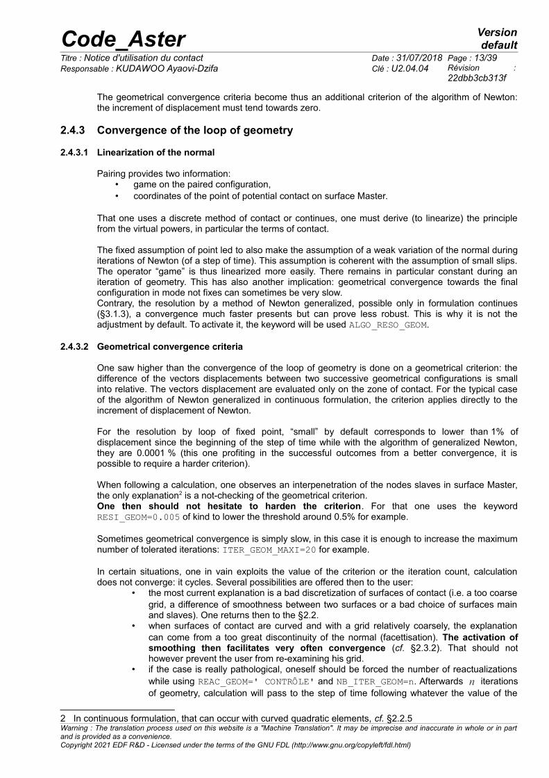
Figure 2.2.3-1: Choice of surfaces main and slaves according to various situations 2.2.4 Orientation of the normals
It is paramount always to direct them normals surfaces of contact so that they are outgoing. One cando it using the operator MODI_MAILLAGE. According to whether surface to be directed is a mesh ofskin of a solid element, a hull or a beam, the keyword respectively will be used ORIE_PEAU_2D orORIE_PEAU_3D, ORIE_NORM_COQUE, ORIE_LIGNE.In the case of ORIE_LIGNE, one directs the tangent, of kind to being able systematically to producethe normal by a vector product. By default (keyword VERI_NORM of DEFI_CONTACT), the good orientation of the normals is checkedand one stops the user if need be.
2.2.5 Smoothness and degree of grid of curved surfaces
When surfaces of contact are curved, it is necessary to guarantee the good continuity of the normal tothe facets. For that, one can is:• to net finely into linear and to use the option of smoothing (cf. §2.3.2)• to net into quadraticSo that the quadratic grid preserves its interest, it is necessary to have placed them nodes mediumson the geometry in the maillor and not to have used the operator CREA_MAILLAGE/LINE_QUAD ofCode_Aster.
Cas Formulation Discrète: In the case of quadratic surfaces of contact, in discrete formulation it is not necessary thatsurfaces of contact consist of quadrangular meshs with 8 nodes (QUAD8) and one will thus preferrather the meshs with 9 nodes (QUAD9). They then will be transformed HEXA20 in HEXA27 and themPENTA15 in PENTA18 (with the operator CREA_MAILLAGE). At present, mixed grids made up at thesame time ofHEXA20 and of PENTA15 are not transformable by CREA_MAILLAGE.
Warning : The translation process used on this website is a "Machine Translation". It may be imprecise and inaccurate in whole or in partand is provided as a convenience.Copyright 2021 EDF R&D - Licensed under the terms of the GNU FDL (http://www.gnu.org/copyleft/fdl.html)

Code_Aster Versiondefault
Titre : Notice d'utilisation du contact Date : 31/07/2018 Page : 10/39Responsable : KUDAWOO Ayaovi-Dzifa Clé : U2.04.04 Révision :
22dbb3cb313f
If however the use of elements HEXA20 prove to be obligatory, Lbe linear relations writtenautomatically on this occasion can be likely to enter in conflict with boundary conditions (in particular ofsymmetry), this is why it can be necessary to impose the boundary conditions only on the nodes topsof the meshs QUAD8 concerned (one will be able to use the operator DEFI_GROUP for the creation ofthe group of ad hoc nodes).
Case continuous formulation: In continuous formulation(ALGO_CONT=' STANDARD'), for meshs of edge curved, the use ofelements QUAD8 or TRIA6 can involve violations of the law of contact : this last is checked onaverage. One then observes games slightly positive or slightly negative in the presence of contact,which can disturb the results close to the zone of contact or calculations in recovery with initial state.For this reason it is advised to use elements HEXA27 or PENTA18 (with faces QUAD9) or many linearelements.
When at the end of a calculation, one notices a strong rate of interpenetration of the main nodes insidesurfaces slaves (what is possible contrary contrary), that generally means that the grid of one or twosurfaces is too coarse or that there is a too great difference of smoothness between the two grids ofsurfaces. One can then either refine, or to reverse main and slave.
If a surface is rigid (and thus main), a coarse grid is sufficient except of course in the curved zones.
Finally in the typical case of one contact cylinder-cylinder or sphere-sphere, it is necessary to takecare of to net each surface sufficiently to avoid leaving too much vacuum between them. Indeed, inCode_Aster, one does not make for the moment not repositioning of nodes nor of projections onsplines passing by surface Master, a too coarse grid will cause one then strong oscillation of thecontact pressure (detection of the contact a node on two).
If there are oscillations on contact pressures due to a strongly incompatible grid in the zone of contact,the method should be privileged ALGO_CONT=' LAC'.
2.2.6 Sharp angles
The algorithms of pairing function less better in the presence of sharp angles, this is why one will asmuch as possible avoid having some in the grid of surfaces Masters and slaves. For example one willprefer to model a leave rather than a sharp angle.
If a sharp angle is essential, one will choose the surface which carries it like slave.
2.2.7 Quality of the grid
The quality of the surface elements which constitute the surface of main contact has a direct impact onthe quality of pairing. Indeed distorted meshs, for example, can harm the precision of projections inspite of the robustness of the algorithm: the unicity of projection is not guaranteed any more.For these reasons, it is recommended to check the quality of the produced grids and if necessary tocorrect their defects. In Code_Aster, the order MACR_INFO_MAIL allows to display the distribution ofthe elements according to their quality.
2.3 Control of pairing
2.3.1 Choice of the type of pairing
In Code_Aster, three types of pairing are available: • “master-slave” (by default): it is generic, it makes it possible to prevent the nodes of surface
slave from penetrating the meshs of surface Master using orthogonal projections of a node ona mesh. It is available for the discrete formulation and the formulation continues(ALGO_CONT=' STANDARD').
Warning : The translation process used on this website is a "Machine Translation". It may be imprecise and inaccurate in whole or in partand is provided as a convenience.Copyright 2021 EDF R&D - Licensed under the terms of the GNU FDL (http://www.gnu.org/copyleft/fdl.html)

Code_Aster Versiondefault
Titre : Notice d'utilisation du contact Date : 31/07/2018 Page : 11/39Responsable : KUDAWOO Ayaovi-Dzifa Clé : U2.04.04 Révision :
22dbb3cb313f
• “nodal”: it makes it possible to prevent the nodes slaves from penetrating the main nodesaccording to a direction (given by the normal slave). It is a pairing reserved for the compatiblegrids of surfaces of contact for calculations in small slips. It is not available in continuousformulation (cf. §3.1.3).
• “ MORTAR ” (by default): it is more qualitative, it allowsto impose the conditions of contact onaverage on the intersected meshs. With this method one reaches precise details ofinterpenetrations lower than 1.E-10 %. It is available only for the formulation continues(ALGO_CONT='LAKE‘).
2.3.2 Smoothing of the normals
As its name indicates it this option makes it possible to smooth the normals. It is particularly useful inthe case of curved surfaces with a grid into linear. This process is founded on average normals with thenodes, then their interpolation starting from the functions of form and realised normals, it makes itpossible to ensure continuity normal with the nodes.
The normal is not then any more the geometrical normal, one will thus take the precaution (advised inany case) to check the results visually well.
A checking of the facettisation of surfaces is carried out automatically at the end of the step of time.She transmits a message of information when this one becomes too important and it is then advised toactivate smoothing.
2.3.3 Choice of the normals: case formulation other than method LAKE
One always advises to leave the values by default: NORMALE=' MAIT', VECT_MAIT=' AUTO'. I.e.the relation of nonpenetration is written starting from the normal Master, determined thanks to the grid.
However there exist some rare situations where one can want to impose the choice of the normal: it isprimarily the treatment of the contact beam-beam (in 2D only) and of the case where surface Master isa mesh of the type POI1. One returns to the §3.1.6 of [U4.44.11] for more details.
2.3.4 Exclusion of nodes slaves of pairing: case formulation other than method LAKE
The keyword SANS_GROUP_NO/SANS_NOEUD serves to exclude from pairing as the nodes slaves.There can be several reasons with that:
• surface Master and slave have a nonempty intersection (bottom of crack, blocking ofmovements of rigid body); the common nodes do not need to be treated by the contact, theymust thus be excluded.
• there already exists on the nodes slaves considered of the linear relations (boundaryconditions, blocking of movements of rigid body); if those interfere with the direction of thecontact (respectively of friction), one in general advises to privilege the boundary conditionsand thus not to solve the contact on these nodes.
A fatal error is emitted when there exist nodes common to surfaces Masters and slaves and that thelatter were not excluded.
2.4 To understand geometrical non-linearity
As one explained, geometrical non-linearity rises owing to the fact that one must apply conditions ofcontact-friction to a geometrical configuration which one does not know. In this section, one makes asmall digression in order to explain the approach adopted to overcome this difficulty.
2.4.1 Assumption of small slips
The phase of pairing is a phase preliminary to the formulation of the conditions of contact to solve. Inpractice, that means:
Warning : The translation process used on this website is a "Machine Translation". It may be imprecise and inaccurate in whole or in partand is provided as a convenience.Copyright 2021 EDF R&D - Licensed under the terms of the GNU FDL (http://www.gnu.org/copyleft/fdl.html)

Code_Aster Versiondefault
Titre : Notice d'utilisation du contact Date : 31/07/2018 Page : 12/39Responsable : KUDAWOO Ayaovi-Dzifa Clé : U2.04.04 Révision :
22dbb3cb313f
• for the discrete methods, the construction of a matrix A (for Pairing) as multiplied by theincrement of displacement u since the paired configuration, it gives the increment of game(linearized).
• for the method continues, association between a point of contact and its project in theparametric space of the mesh Master paired. It is by bringing up to date the coordinates of themesh Master with displacement u that obtains it the new coordinates (linearized) of theproject.
Just as the equilibrium conditions, the conditions of contact are expressed on the deformedconfiguration (or finale). This configuration is not known a priori.The assumption of weak relative slips of surfaces in contact is the analogue of the assumption of smalldisturbances (for the writing of the relations of balance).
It consists in saying that the final configuration of surfaces in contact is not very different from the initialconfiguration, which thus makes it possible to once and for all carry out pairing at the beginning ofcalculation on the initial configuration. Then to use the conditions established on this configuration forall calculation.
Such a problem is then linear geometrically: only the non-linearity of contact-friction remains, it istreated with adapted algorithms (cf. section 3).
2.4.2 Case general
To deal with problems of great relative slips of surfaces in contact, two possibilities exist: the use of afixed loop of point to be reduced to the cases of small slips or for the formulation continues (§3.1.3) thesimultaneous resolution within the algorithm of Newton.
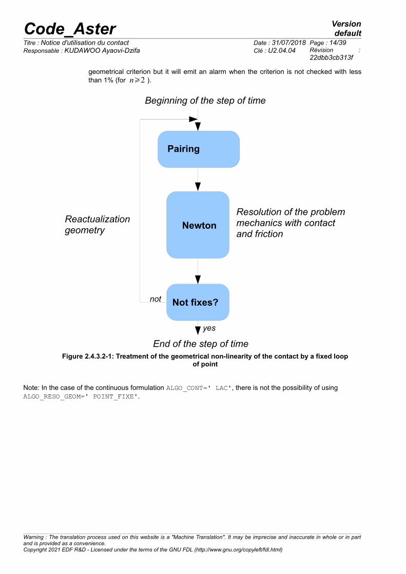
2.4.2.1 Buckle of point fixes (ALGO_RESO_GEOM=' POINT_FIXE')
The adopted approach is very similar to the resolution of a non-linear problem by the method ofNewton. One transforms a geometrical non-linear problem into a succession of geometricallinear problems. For that one will solve a succession of problems on the assumption of small slips.
I.e. one carries out a pairing (on a balanced initial configuration) and a resolution of Newton (withresolution of the contact as one will explain it in the section 3). This gives us a new configuration; if thisconfiguration is “close” to the initial configuration then one converged (it was thus the finalconfiguration), if not one buckles: one remakes a pairing then a resolution… and so on until finding theconfiguration final (cf. Figure 2.4.3.2-1).
The difficulty is in the characterization of the convergence of this process of fixed point. What two“close” configurations? In Code_Aster, they are two configurations of which the“mechanical” vector displacement to pass from the one to the other (i.e. the increment of displacementobtained by Newton restricted to the degrees of freedom DX, DY, DZ) has a small infinite standard infront of the infinite standard of the vector preceding displacement.
That implies that one thus makes always at least two iterations of geometry with this criterion (in orderto give a vector initial displacement). One returns in paragraph 3.7 of [R5.03.50] for the exactexpression of the infinite standard.
2.4.2.2 Algorithm of generalized Newton (ALGO_RESO_GEOM=' NEWTON')
The formulation continues (§3.1.3) offer the possibility of treating geometrical non-linearity directlywithin the algorithm of Newton. For that a pairing is carried out with each iteration and the geometricalterms of the tangent matrix are also reactualized.
Warning : The translation process used on this website is a "Machine Translation". It may be imprecise and inaccurate in whole or in partand is provided as a convenience.Copyright 2021 EDF R&D - Licensed under the terms of the GNU FDL (http://www.gnu.org/copyleft/fdl.html)
Code_Aster Versiondefault
Titre : Notice d'utilisation du contact Date : 31/07/2018 Page : 13/39Responsable : KUDAWOO Ayaovi-Dzifa Clé : U2.04.04 Révision :
22dbb3cb313f
The geometrical convergence criteria become thus an additional criterion of the algorithm of Newton:the increment of displacement must tend towards zero.
2.4.3 Convergence of the loop of geometry
2.4.3.1 Linearization of the normal
Pairing provides two information:• game on the paired configuration,• coordinates of the point of potential contact on surface Master.
That one uses a discrete method of contact or continues, one must derive (to linearize) the principlefrom the virtual powers, in particular the terms of contact.
The fixed assumption of point led to also make the assumption of a weak variation of the normal duringiterations of Newton (of a step of time). This assumption is coherent with the assumption of small slips.The operator “game” is thus linearized more easily. There remains in particular constant during aniteration of geometry. This has also another implication: geometrical convergence towards the finalconfiguration in mode not fixes can sometimes be very slow.Contrary, the resolution by a method of Newton generalized, possible only in formulation continues(§3.1.3), a convergence much faster presents but can prove less robust. This is why it is not theadjustment by default. To activate it, the keyword will be used ALGO_RESO_GEOM.
2.4.3.2 Geometrical convergence criteria
One saw higher than the convergence of the loop of geometry is done on a geometrical criterion: thedifference of the vectors displacements between two successive geometrical configurations is smallinto relative. The vectors displacement are evaluated only on the zone of contact. For the typical caseof the algorithm of Newton generalized in continuous formulation, the criterion applies directly to theincrement of displacement of Newton.
For the resolution by loop of fixed point, “small” by default corresponds to lower than 1% ofdisplacement since the beginning of the step of time while with the algorithm of generalized Newton,they are 0.0001 % (this one profiting in the successful outcomes from a better convergence, it ispossible to require a harder criterion).
When following a calculation, one observes an interpenetration of the nodes slaves in surface Master,the only explanation2 is a not-checking of the geometrical criterion.One then should not hesitate to harden the criterion. For that one uses the keywordRESI_GEOM=0.005 of kind to lower the threshold around 0.5% for example.
Sometimes geometrical convergence is simply slow, in this case it is enough to increase the maximumnumber of tolerated iterations: ITER_GEOM_MAXI=20 for example.
In certain situations, one in vain exploits the value of the criterion or the iteration count, calculationdoes not converge: it cycles. Several possibilities are offered then to the user:
• the most current explanation is a bad discretization of surfaces of contact (i.e. a too coarsegrid, a difference of smoothness between two surfaces or a bad choice of surfaces mainand slaves). One returns then to the §2.2.
• when surfaces of contact are curved and with a grid relatively coarsely, the explanationcan come from a too great discontinuity of the normal (facettisation). The activation ofsmoothing then facilitates very often convergence (cf. §2.3.2). That should nothowever prevent the user from re-examining his grid.
• if the case is really pathological, oneself should be forced the number of reactualizationswhile using REAC_GEOM=' CONTRÔLE' and NB_ITER_GEOM=n. Afterwards n iterationsof geometry, calculation will pass to the step of time following whatever the value of the
2 In continuous formulation, that can occur with curved quadratic elements, cf. §2.2.5Warning : The translation process used on this website is a "Machine Translation". It may be imprecise and inaccurate in whole or in partand is provided as a convenience.Copyright 2021 EDF R&D - Licensed under the terms of the GNU FDL (http://www.gnu.org/copyleft/fdl.html)
Code_Aster Versiondefault
Titre : Notice d'utilisation du contact Date : 31/07/2018 Page : 14/39Responsable : KUDAWOO Ayaovi-Dzifa Clé : U2.04.04 Révision :
22dbb3cb313f
geometrical criterion but it will emit an alarm when the criterion is not checked with lessthan 1% (for n2 ).
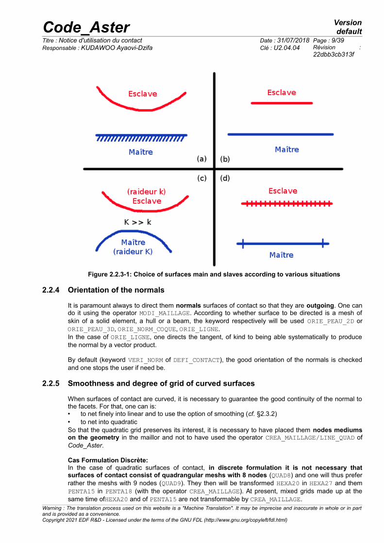
Figure 2.4.3.2-1: Treatment of the geometrical non-linearity of the contact by a fixed loopof point
Note: In the case of the continuous formulation ALGO_CONT=' LAC', there is not the possibility of using ALGO_RESO_GEOM=' POINT_FIXE'.
Warning : The translation process used on this website is a "Machine Translation". It may be imprecise and inaccurate in whole or in partand is provided as a convenience.Copyright 2021 EDF R&D - Licensed under the terms of the GNU FDL (http://www.gnu.org/copyleft/fdl.html)
Beginning of the step of time
End of the step of time
Reactualizationgeometry
Resolution of the problemmechanics with contactand friction
Newton
Not fixes?not
yes
Pairing

Code_Aster Versiondefault
Titre : Notice d'utilisation du contact Date : 31/07/2018 Page : 15/39Responsable : KUDAWOO Ayaovi-Dzifa Clé : U2.04.04 Révision :
22dbb3cb313f
3 Resolution
3.1 Outline general of the algorithm of resolution
3.1.1 Definition and general remarks
What one calls “resolution of the contact”, it is the operation consisting in solving the system formed bythe juxtaposition of the classical equations of the mechanics and the equations of contact-friction (thegeometrical aspect being treated by pairing, it remains at this stage only the non-linearity of thresholdof friction and the non-linearity of statute of the contact).
It should be noted that the two formulations available in the code differ notably on this point. Withoutgoing into the details, one briefly explains these differences for the continuation.
If the formulations discrete and continuous amount well solving the same physical problem, as theirname indicates it they do not formulate it numerically same manner. One presents in a synthetic waythe differences between these two formulations.
Case discrete formulation. EN formulation discrete, the conditions of contact-friction are applied to the discretized system thanksto “under-iterations” of Newton. In a standard iteration of Newton there are two stages: initially, ONcalculate that the resolution of the linear system obtained by Newton Ku= f with the initial conditionsof contact then in the second time by various methods of optimization under constraints condensed onthe zone of contact, the conditions are solved ofinequalities of contact. This second phase makes itpossible to recompute the “true” pressures of contact. For the following iteration of Newton, onemodifies the second member of kind to being able to take into account new conditions of contactresulting from the second phase. For the discrete penalization, one also modifies the matrix K to limitthe interpenetrations. This technique makes it possible to solve in a powerful way of the problems withweak ddls of contact. One can say that the discrete formulation imposes in an algebraic way theconditions of contact without building a continuous element for contact.
Case formulation continuous . EN formulation continue, one writes a variational formulation mixed for to take equations of contact-friction. The variational formulation is of Lagrangian type classical for the method LAKE, Lagrangianincreased for the method STANDARD and Lagrangian penalized for the method PENALIZATION. Theapproach adopted to solve the non-linear system is to create late elements continuous of contact.These late elements of contact carry ddls of master-slave displacement as well as multipliers ofLagrange only with dimensions slave. With the execution of DEFI_CONTACT, it is created in atransparent way to the user of the couples of contact making it possible to potentially describe the ddlsaccording to the topology of the meshs contacting. In the same way, at the time of the resolution inSTAT_NON_LINE, it is created elements continuous by couple contact who allow the calculation ofthe matrices and elementary vectors which will be assembled with the total rigidity of the mechanicalsystem. A standard iteration of Newton thus provides to each resolution of displacements but also ofthe multipliers of Lagrange (LAGS_C). The main advantage of the continuous method is to propose viathe degree of freedom LAGS_C (in the field DEPL) access to the contact pressure on surface slave.One however draws attention to the fact that this quantity is in fact onlya density of force of contactper unit of area expressed on the configuration of reference. In particular, in great deformations,one cannot any more qualify it pressure because it does not have any more a physical direction.Because of size of the system, the formulation continues is often less powerful than the discrete butmore robust and more qualitative formulation in various situations (plasitcité+contact for example).
3.1.2 Discrete formulation
Warning : The translation process used on this website is a "Machine Translation". It may be imprecise and inaccurate in whole or in partand is provided as a convenience.Copyright 2021 EDF R&D - Licensed under the terms of the GNU FDL (http://www.gnu.org/copyleft/fdl.html)
Code_Aster Versiondefault
Titre : Notice d'utilisation du contact Date : 31/07/2018 Page : 16/39Responsable : KUDAWOO Ayaovi-Dzifa Clé : U2.04.04 Révision :
22dbb3cb313f
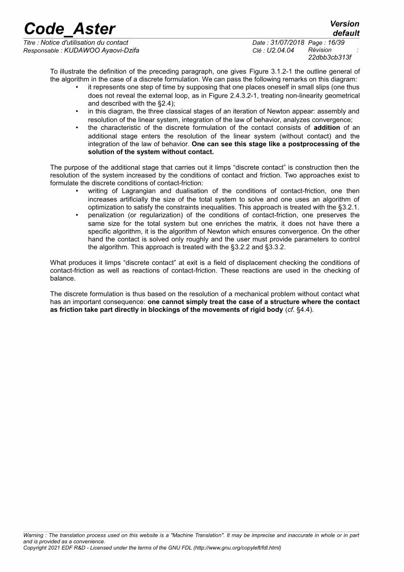
To illustrate the definition of the preceding paragraph, one gives Figure 3.1.2-1 the outline general ofthe algorithm in the case of a discrete formulation. We can pass the following remarks on this diagram:
• it represents one step of time by supposing that one places oneself in small slips (one thusdoes not reveal the external loop, as in Figure 2.4.3.2-1, treating non-linearity geometricaland described with the §2.4);
• in this diagram, the three classical stages of an iteration of Newton appear: assembly andresolution of the linear system, integration of the law of behavior, analyzes convergence;
• the characteristic of the discrete formulation of the contact consists of addition of anadditional stage enters the resolution of the linear system (without contact) and theintegration of the law of behavior. One can see this stage like a postprocessing of thesolution of the system without contact.
The purpose of the additional stage that carries out it limps “discrete contact” is construction then theresolution of the system increased by the conditions of contact and friction. Two approaches exist toformulate the discrete conditions of contact-friction:
• writing of Lagrangian and dualisation of the conditions of contact-friction, one thenincreases artificially the size of the total system to solve and one uses an algorithm ofoptimization to satisfy the constraints inequalities. This approach is treated with the §3.2.1.
• penalization (or regularization) of the conditions of contact-friction, one preserves thesame size for the total system but one enriches the matrix, it does not have there aspecific algorithm, it is the algorithm of Newton which ensures convergence. On the otherhand the contact is solved only roughly and the user must provide parameters to controlthe algorithm. This approach is treated with the §3.2.2 and §3.3.2.
What produces it limps “discrete contact” at exit is a field of displacement checking the conditions ofcontact-friction as well as reactions of contact-friction. These reactions are used in the checking ofbalance.
The discrete formulation is thus based on the resolution of a mechanical problem without contact whathas an important consequence: one cannot simply treat the case of a structure where the contactas friction take part directly in blockings of the movements of rigid body (cf. §4.4).
Warning : The translation process used on this website is a "Machine Translation". It may be imprecise and inaccurate in whole or in partand is provided as a convenience.Copyright 2021 EDF R&D - Licensed under the terms of the GNU FDL (http://www.gnu.org/copyleft/fdl.html)
Code_Aster Versiondefault
Titre : Notice d'utilisation du contact Date : 31/07/2018 Page : 17/39Responsable : KUDAWOO Ayaovi-Dzifa Clé : U2.04.04 Révision :
22dbb3cb313f
Figure 3.1.2-1: Algorithm general of a step of time in discrete formulation (small slips)
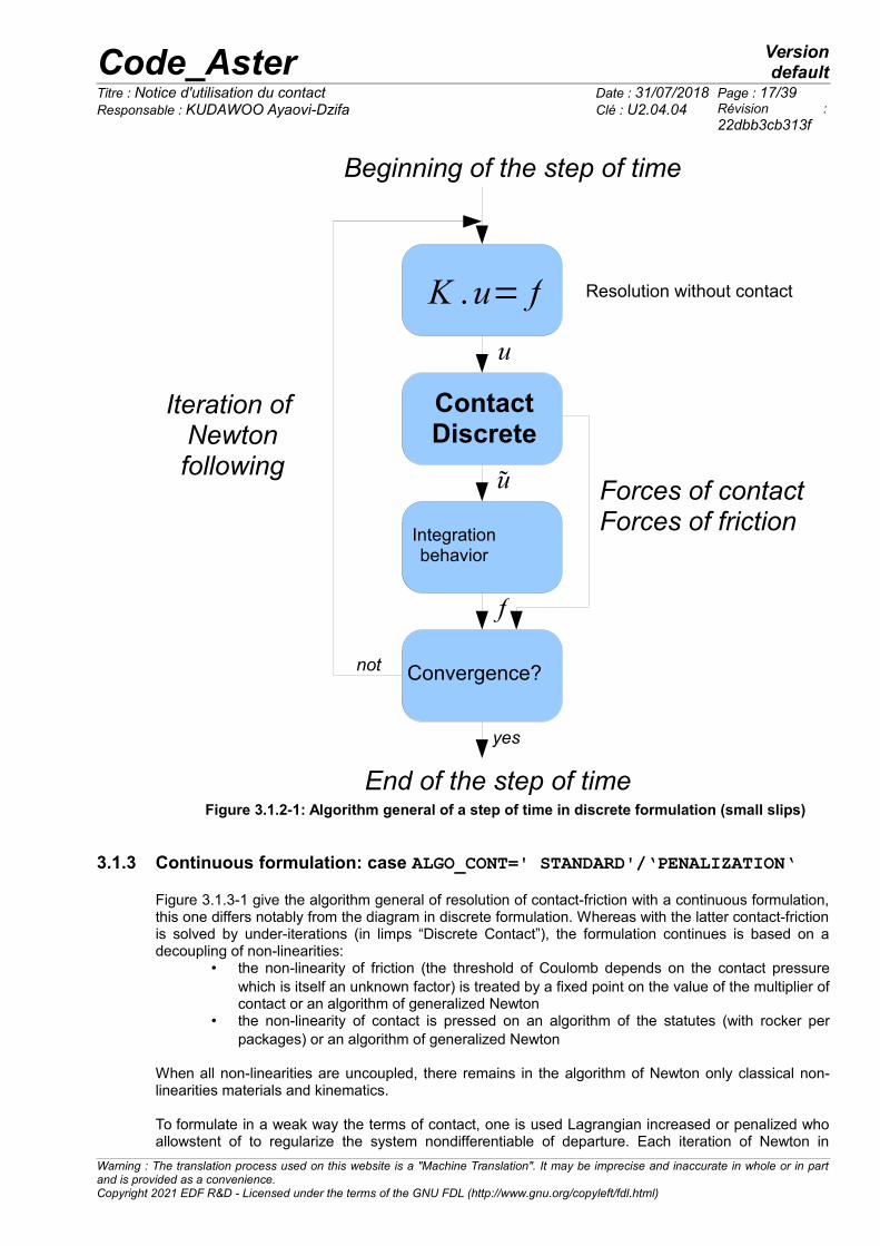
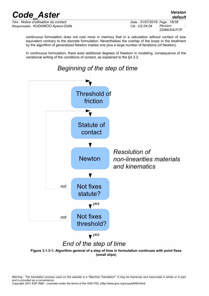
3.1.3 Continuous formulation: case ALGO_CONT=' STANDARD'/‘PENALIZATION‘
Figure 3.1.3-1 give the algorithm general of resolution of contact-friction with a continuous formulation,this one differs notably from the diagram in discrete formulation. Whereas with the latter contact-frictionis solved by under-iterations (in limps “Discrete Contact”), the formulation continues is based on adecoupling of non-linearities:
• the non-linearity of friction (the threshold of Coulomb depends on the contact pressurewhich is itself an unknown factor) is treated by a fixed point on the value of the multiplier ofcontact or an algorithm of generalized Newton
• the non-linearity of contact is pressed on an algorithm of the statutes (with rocker perpackages) or an algorithm of generalized Newton
When all non-linearities are uncoupled, there remains in the algorithm of Newton only classical non-linearities materials and kinematics.
To formulate in a weak way the terms of contact, one is used Lagrangian increased or penalized whoallowstent of to regularize the system nondifferentiable of departure. Each iteration of Newton in
Warning : The translation process used on this website is a "Machine Translation". It may be imprecise and inaccurate in whole or in partand is provided as a convenience.Copyright 2021 EDF R&D - Licensed under the terms of the GNU FDL (http://www.gnu.org/copyleft/fdl.html)
Beginning of the step of time
End of the step of time
K .u= f
ContactDiscrete
Iteration of Newtonfollowing
u Forces of contactForces of friction
Integrationbehavior
Convergence?
u
not
yes
Resolution without contact
f
Code_Aster Versiondefault
Titre : Notice d'utilisation du contact Date : 31/07/2018 Page : 18/39Responsable : KUDAWOO Ayaovi-Dzifa Clé : U2.04.04 Révision :
22dbb3cb313f
continuous formulation does not cost more in memory that in a calculation without contact of sizeequivalent contrary to the discrete formulation. Nevertheless the overlap of the loops or the treatmentby the algorithm of generalized Newton implies one plus a large number of iterations (of Newton).
In continuous formulation, there exist additional degrees of freedom in modeling, consequence of thevariational writing of the conditions of contact, as explained to the §4.3.2.
Figure 3.1.3-1: Algorithm general of a step of time in formulation continues with point fixes(small slips)
Warning : The translation process used on this website is a "Machine Translation". It may be imprecise and inaccurate in whole or in partand is provided as a convenience.Copyright 2021 EDF R&D - Licensed under the terms of the GNU FDL (http://www.gnu.org/copyleft/fdl.html)
Beginning of the step of time
End of the step of time
Resolution ofnon-linearities materialsand kinematics
Not fixesstatute?
not
yes
Not fixesthreshold?
not
yes
Newton
Threshold offriction
Statute ofcontact

Code_Aster Versiondefault
Titre : Notice d'utilisation du contact Date : 31/07/2018 Page : 19/39Responsable : KUDAWOO Ayaovi-Dzifa Clé : U2.04.04 Révision :
22dbb3cb313f
In continuous formulation, two algorithms exist to control the variables specific to the contact (internalvariables by analogy with the laws of behavior) :
• method of point fixes on the statutes of contact: the state of the statutes of contact isevaluated in an external loop with the loop of Newton. To choose the algorithm, should beused the total keyword ALGO_RESO_CONT= ' POINT_FIXE'. The method of the pointfixes (ALGO_RESO_CONT=' POINT_FIXE') is most robust but also most expensive sincethe non-linear problem (plasticity for example) is solved with each change of the statutesof contact.
• method of Newton generalized: the statutes of contact are evaluated with each iteration ofNewton (it is the defect). Method of Newton generalized (ALGO_RESO_CONT=' NEWTON')is more powerful but poses sometimes problems of convergence. The keywordADAPTATION allows to make robust this mode of convergence. If one does not manage toconverge on the statutes in spite of the keyword ADAPTATION, it is necessary to returnwith a method of point fixed.
3.1.4 Continuous formulation: case ALGO_CONT='LAKE‘
This method makes it possible to solve in a way realised the pressures and the games on the meshsintersected of contact. She belongs to the family of the methods of the type MORTAR which arefamous for their capacities to deal with problems of interface in mechanics. She has meaning only byelement of contact. The dependent problems other than redundant nodes for the formulation continuesstandard/penalized with the boundary conditions is not a problem for this method since the conditionsof contact are not imposed on the nodes but by element.
The method LAKE ( Room Average Contact ) do not use a fixed loop of point. All nonthe linearitiesof contact (statuts+geometry) can vary from an iteration of Newton to the other. Only the convergencecriteria make it possible to control the quality of resolution of contact. At present the method LAKE doesnot solve friction yet.
Lastly, to use the method LAKE, it is necessary to carry out a phase of preprocessing of grid(CREA_MAILLAGE/DECOUPE_LAC) who consists in preparing the “patchs” slaves for the conditions ofcontact checked by macro-mesh.
3.1.5 Continuous formulation: treatment of the incompatibilities.
Dyears the case of the grids where the incompatibility is weak, one can use the standard/penalizedcontinuous methods. To realize of the influence of the compatibility of grid one can activate under thekeyword ZONE of DEFI_CONTACT a keyword which reduces the oscillations of contact pressures:INTEGRATION. The keyword has two disadvantages however: the number of active statutes of contactis not available at the end of each increment calculation and moreover there is not CONT_NOEU at theend of calculation. It is thus necessary to be folded back on postprocessing with CALC_PRESSION. Inthe case of strong incompatibilities of grid, the method LAKE makes it possible to have a good qualityof contact pressures.
On the example of the analytical CAS-test “patch-test of Taylor” ssnp170 (parallelepipedic contactbetween two blocks with analytical pressure of -25MPa), one notices that according to the parametersetting of the integration of the contact terms, the oscillations disappear or not.
Warning : The translation process used on this website is a "Machine Translation". It may be imprecise and inaccurate in whole or in partand is provided as a convenience.Copyright 2021 EDF R&D - Licensed under the terms of the GNU FDL (http://www.gnu.org/copyleft/fdl.html)

Code_Aster Versiondefault
Titre : Notice d'utilisation du contact Date : 31/07/2018 Page : 20/39Responsable : KUDAWOO Ayaovi-Dzifa Clé : U2.04.04 Révision :
22dbb3cb313f
Type integration Visualization of the nodal constraints
CAR
NCOTES
LAKE
Warning : The translation process used on this website is a "Machine Translation". It may be imprecise and inaccurate in whole or in partand is provided as a convenience.Copyright 2021 EDF R&D - Licensed under the terms of the GNU FDL (http://www.gnu.org/copyleft/fdl.html)

Code_Aster Versiondefault
Titre : Notice d'utilisation du contact Date : 31/07/2018 Page : 21/39Responsable : KUDAWOO Ayaovi-Dzifa Clé : U2.04.04 Révision :
22dbb3cb313f
3.2 Resolution of a problem with contact alone 3.2.1 Dualisation in discrete formulation (FORMULATION=' DISCRETE')
3.2.1.1 Principle
The dualisation of the discrete system consists of the introduction of Lagrangian (cf [R5.03.50]). Thesystem to be solved takes the following shape when it is tiny room on the active connections:
{C . uAcT . i=F i
Ac . u=d i−1 (1)
Knowing that the resolution of the system without contact was already carried out, one knows thesolution of the following system:
C .u=F i (2)
The technique of resolution is based then on the use of the complement of Schur of the system (1) totransform the system:
S schur=−Ac .C−1.( Ac )
T (3)
The problem thus transformed has the size amongst nodes slaves and it is full. Two algorithms with thechoice are available to deal with this new problem:
• a method of active constraints (ALGO_CONT=' CONTRAINTE') being based onconstruction explicit and the factorization of the complement of Schur
• a method of gradient combined project (ALGO_CONT=' GCP') being based on theresolution iterative system formed by the complement of Schur of the system
It should be noted that the dualisation requires the use of a direct linear solvor: in Code_Aster, thatmeans ‘MULT_FRONT’ or ‘MUMPS’.Each of the 2 algorithms quoted above indeed carries out under-iterations during which it is necessaryto solve the linear system (2) with C the matrix of rigidity of the total system without contact (what ismuch faster if C is already factorized).
3.2.1.2 Method ‘FORCED’
Being based on a factorization (thus a direct solvor) to solve the system associated with thecomplement with Schur, the method ‘FORCED’ do not ask any parameter setting. In addition itsconvergence3 is shown, which explains why it is the method by default in the presence of contact.
Nevertheless the use of a direct solvor presents a major drawback: this algorithm is not adapted assoon as the number of nodes slaves exceeds a few hundreds (500). Indeed the factorization of afull matrix very quickly becomes crippling.
The construction of the complement of Schur can be accelerated by using the parameter NB_RESOL(cf. [U4.44.11], value by default 10) to the detriment of the consumed memory (the larger the number ofdegrees of freedom total is, the more the increase of this parameter is expensive). In order to optimizea calculation with the method of the active constraints, it is advised to do a calculation on a step of timein order to to find a compromise time/memory (cf. [U1.03.03] for the reading of information on theconsumed memory).
3 One uses a direct solvor well to build the complement of Schur but the method of the active constraintsconsists in activating or to one by one disable the connections of contact until satisfying the total system, it isthus an iterative algorithm.
Warning : The translation process used on this website is a "Machine Translation". It may be imprecise and inaccurate in whole or in partand is provided as a convenience.Copyright 2021 EDF R&D - Licensed under the terms of the GNU FDL (http://www.gnu.org/copyleft/fdl.html)

Code_Aster Versiondefault
Titre : Notice d'utilisation du contact Date : 31/07/2018 Page : 22/39Responsable : KUDAWOO Ayaovi-Dzifa Clé : U2.04.04 Révision :
22dbb3cb313f
3.2.1.3 Method ‘GCP’
When that one cannot use the method of contact by default any more because it is too expensive, analternative is the use of the method ‘GCP’. As one mentioned above this method consists of theapplication of an iterative solvor (gradient combined project) to solve the dual problem.The main advantage of such a method is not to be more limited in the face of problem (severalthousands of nodes slaves are perfectly atteignables). The counterpart, specific to any iterative solvor,is an obligatory parameter setting for the user.This method is usable in parallel calculation, it is besides the only discrete method with reallybenefitting from it.
Like any iterative solvor, method ‘GCP’ use convergence criteria: it is about a criterion on the value ofthe game. Given by the keyword RESI_ABSO, it controls the tolerated maximum interpenetration.It is obligatory and is expressed in the same unit as that used for the grid. One advises to initially use acriterion equal to 10−3 time average interpenetration when the contact is not taken into account (cf§4.8).
If one notes difficulties of convergence of the algorithm of the gradient combined project, there exist 2parameters which, one advises to exploit (in an additive way, i.e. one then the other):
• to use an not-acceptable linear research (RECH_LINEAIRE=' NON_ADMISSIBLE')• to use a pre-conditioner of Dirichlet (PRE_COND=' DIRICHLET')
The pre-conditioner has the advantage of being optimal and thus decreases appreciably the iterationcount necessary to convergence. Moreover when one is close to the solution, it makes it possible tomake decrease the residue very quickly and thus to reach very weak criteria of interpenetrations.Its disadvantage is high costs which can often prevent a saving of time of calculation in spite of thereduction amongst iterations.For this reason, it is possible to ask its activation only when the residue sufficiently decreased: the pre-conditioner then makes it possible ideally to converge in some iterations. The difficulty lies in thequantification of “sufficiently decreased” or in other words vicinity of the solution. One controls thisrelease by the keyword COEF_RESI who is the coefficient (lower than 1) by which it is necessary tohave multiplied the initial residue (initial maximum interpenetration thus) before applying the pre-conditioner. An example of implementation of this parameter is given in CAS-test SSNA102E.
3.2.2 Penalization in discrete formulation: algorithm ‘PENALIZATION’
The penalization consists in regularizing the problem of contact: instead of seeking to solve exactly theconditions on the game and the pressure, one introduces a univocal approximate relation which impliesthat an interpenetration will be always observed when the contact is established.
Warning : The translation process used on this website is a "Machine Translation". It may be imprecise and inaccurate in whole or in partand is provided as a convenience.Copyright 2021 EDF R&D - Licensed under the terms of the GNU FDL (http://www.gnu.org/copyleft/fdl.html)

Code_Aster Versiondefault
Titre : Notice d'utilisation du contact Date : 31/07/2018 Page : 23/39Responsable : KUDAWOO Ayaovi-Dzifa Clé : U2.04.04 Révision :
22dbb3cb313f
Figure 3.2.2-1: Condition of contact (on the left) and regularization (on the right)
Like shows it Figure 3.2.2-1 a parameter is added E_N to regularize the condition of contact: the largerit is, the more one tends towards the exact condition, the more it is small, the more one toleratesinterpenetration.In discrete formulation, the concept of contact pressure does not exist because one reasons on thenodes of the grid finite element: one thus works with nodal forces (cf. §4.3). The coefficient E_N known
as of penalization thus the dimension of a stiffness has ( N.m−1 ). One generally makes the analogy between the coefficient of penalization and the stiffness of unilateralsprings which one would place between surface Master and slave where interpenetration is observed.
One generally chooses E_N by successive tests: • first of all one will start by taking a value equalizes with 10 times the largest Young
modulus of the structure multiplied by a length characteristic of this one;• if calculation gives a result (satisfying or not), one will each time increase then the value
by multiplying it by 10 until getting a stable result in terms of displacements and especiallyin terms of constraints.
The advantage of the method of penalization is not to increase the size of the system contrary tothe dualisation, but also not to restrict the choice of the linear solvor. The counterpart is asensitivity to the coefficient of penalization which implies systematically to conduct a parametric studybefore launching out in long calculations (cf. [U1.04.00] and [U2.08.07] for the launching of distributedparametric calculations).
To help to gauge the coefficient of penalization, there exists an automatic adaptation mechanism beingbased on the order DEFI_LIST_INST [U4.34.03]. One will find an example of implementation in CAS-test SDNV103I [V5.03.103].
3.2.3 Formulation ‘CONTINUOUS’: council on the solveurs and parallelism
For the problem of contact alone, the method continues has the advantage like the method (discrete) ofthe active constraints of not requiring any adjustment by the user.
Moreover, Comme it is not dependent on a solvor linear direct, it is possible to use a solvor lineariterative (like ‘GCPC’ or ‘PETSC’) to gain enormously over the computing time. However, insofar asthe iterative solveurs can prove less robust, one does not advise to turn to such a solvor that once
Warning : The translation process used on this website is a "Machine Translation". It may be imprecise and inaccurate in whole or in partand is provided as a convenience.Copyright 2021 EDF R&D - Licensed under the terms of the GNU FDL (http://www.gnu.org/copyleft/fdl.html)
Pressure Pressure
Game Game
E_N

Code_Aster Versiondefault
Titre : Notice d'utilisation du contact Date : 31/07/2018 Page : 24/39Responsable : KUDAWOO Ayaovi-Dzifa Clé : U2.04.04 Révision :
22dbb3cb313f
calculation with contact-friction was developed and validated. In any event, it is strongly to advise toreturn to a direct solvor in the event of difficulties of convergence.
When one uses an iterative solvor with the formulation continues contact-friction, it is advisedto activate the method of Newton-Krylov (cf. keyword METHOD of STAT_NON_LINE [U4.51.03])which makes it possible to adapt the convergence criteria of the solvor automatically linear.
3.2.4 Other advices in parallelism
If the user decides to use NORMALE=' ESCL'/‘MAIT_ESCL’ then, parallelism is not available.
In the event of use of implicit DYNA_NON_LINE + DEFI_CONTACT/continue, one imposes that thedistribution is centraliséePour the formulations, discrete one forces to use inAFFE_MODELE/DISTRIBUTION=' CENTRALISE'.
For the formulations, discrete one forces to use in AFFE_MODELE/DISTRIBUTION=' CENTRALISE'.
3.3 Resolution of a problem with friction
3.3.1 Treatment of the non-linearity of threshold
In Code_Aster, the only model of friction available is that of Coulomb (cf [R5.03.50]). An additional non-linearity must be treated in the presence of friction: it is the non-linearity of threshold.The threshold of friction depends indeed on the contact pressure which is itself unknown.The law of Coulomb utilizes a coefficient , called coefficient of Coulomb. During the phase known asof adherence, a point in contact does not move (it has a worthless speed and there exists a tangentialreaction). During the phase of slip, the point has a nonworthless speed and is subjected to a tangentialreaction equalizes with time normal reaction.
In general, if the coefficient of friction is very low, it is advised to neglect frictions. In addition, it isadvised in the studies not to treat initially that the contact, this in order to introduce non-linearitiesones after the others.
The discrete methods that they work by penalization or dualisation press on algorithms dedicated in thepresence of friction (distinct from those used for the contact) while the method continues penalizedstandard/ use two different algorithms:
• method of point fixes on the thresholds of friction: the threshold is brought up to date in anexternal loop with the loop of Newton (and with the loop on the statutes of contact);ALGO_RESO_FROT=' POINT_FIXE'.
• method of Newton generalized: the non-linearity of friction is treated in the process ofNewton, by explicit derivation of all the non-linear terms. ALGO_RESO_FROT=' NEWTON'.
3.3.2 Discrete formulation: penalization of friction (algorithm ‘PENALIZATION‘)
For the 3D problems or of big size, it is advised to deal with the problem of friction by penalization. Thatrequires, as for the penalization of the contact, the entry of a parameter of penalization (E_T). Moredifficult to choose than its equivalent E_N, it requires to carry out a small parametric study.
To make the analogy with the case of the penalization of the contact it will be noticed that the phase ofadherence strictly speaking disappears (as soon as the contact is activated there is interpenetration, infriction there is always slip). Convergence can also be accelerated by the use of the keyword COEF_MATR_FROT.
Warning : The translation process used on this website is a "Machine Translation". It may be imprecise and inaccurate in whole or in partand is provided as a convenience.Copyright 2021 EDF R&D - Licensed under the terms of the GNU FDL (http://www.gnu.org/copyleft/fdl.html)

Code_Aster Versiondefault
Titre : Notice d'utilisation du contact Date : 31/07/2018 Page : 25/39Responsable : KUDAWOO Ayaovi-Dzifa Clé : U2.04.04 Révision :
22dbb3cb313f
3.3.3 Formulation ‘CONTINUOUS‘: STANDARD/PENALISATION.
It is the method of choice when one must deal with a problem of contact-friction : it is mostrobust moreover it tolerates well the great coefficients of friction (larger than 0,3 ).
It is possible to choose among two algorithms of resolution for to fix the internal variables specific to thecontactfriction with the keyword ALGO_RESO_XXXX (XXXX=CONT/FROT).
The method of the point fixes (ALGO_RESO_XXXX= ' POINT_FIXE') is robust but expensive. Methodof Newton generalized (ALGO_RESO_FROT=' NEWTON', by default choice) is very powerful and offersa good level of robustness. The large advantage of this algorithm is its least dependence with the valueof the coefficient of friction, since there is no loop on the thresholds. One produces a not-symmetricalmatrix tangent, which represents a light overcost during factorization and limit the range of the iterativesolveurs usable.
It is preferable to use the generalized method of Newton since the coefficient of friction is notnegligible. The savings of time calculation are very important (up to 80% of profit compared to the fixedpoint).
Two algorithms ‘POINT_FIXE’/‘NEWTON’ give identical results.
When however difficulties of convergence appear, in particular in the presence of important slips, theuser will be able to parameterize the coefficient COEF_FROT (which has the dimension of the reverse ofa distance). This parameter takes a value of 100 by defaults: one will test values understood enters
10−6 and 106 . For studies where adherence is dominating, one will support values of COEF_FROTlower than the value by default while for cases where the slip is dominating, one will choose highervalues. There exist alternatives to the parameter setting into hard of COEF_CONT or COEF_FROT : theyare the adaptive methods.
- A first solution of help is to privilege the method of continuous penalization with the adaptive methods(ALGO_CONT=' PENALISATION'/ADAPTATION=' TOUT'). Indeed, it to activate an automaticalgorithm of check D is possibleU coefficient of penalization (via the analysis of cyclings). If one wantsonly to control the coefficient of penalization without the statutes of contact then ON will use thekeyword ADAPTATION=‘ADAPT_COEF‘. This method can fail in the direction where control can not beeffective, but it will act only on the speed of convergence and not on the quality of the results.Alternative options exist to circumvent the problems of convergence with friction:- To activate the exact resolution of the contact and the penalized resolution of friction and to initiallylimit the number of reactualization geometrical: ALGO_RESO_GEOM=' CONTRÔLE',ZONE/ALGORITHME_CONT=' STANDARD'+ALGORITHME_FROT=' PENALISATION'.- If the technique above did not go: to think of using ADAPTATION=' TOUT' in the keyword ZONE totreat at the same time the cycling and the adaptation of the coefficients of regularization.- There exists a mode which is activated as soon as the keyword ADAPTATION is active: it is it FLIP-FLOP. It makes it possible to declare convergence in statute of contact as soon as the contact pressureis stabilized in the zone of contact. This pressure is an arithmetic mean of contact pressures of all thezones.
3.4 Summary for the choice of the methods of resolution
3.4.1 For contact-friction
For the problems with low number of degrees of freedom in contact (lower than 1000 degrees offreedom), one will privilege a discrete formulation with algorithm of the active constraints (‘FORCED’).If friction must be activated, one will turn to a formulation ‘CONTINUES’.
For the problems with a large number of degrees of freedom in contact (higher than 1000 degrees offreedom), the iterative algorithm of resolution by active constraints ‘GCP’ is most suitable. If however
Warning : The translation process used on this website is a "Machine Translation". It may be imprecise and inaccurate in whole or in partand is provided as a convenience.Copyright 2021 EDF R&D - Licensed under the terms of the GNU FDL (http://www.gnu.org/copyleft/fdl.html)

Code_Aster Versiondefault
Titre : Notice d'utilisation du contact Date : 31/07/2018 Page : 26/39Responsable : KUDAWOO Ayaovi-Dzifa Clé : U2.04.04 Révision :
22dbb3cb313f
one must take into account friction, one will be able to turn once again to the formulation‘CONTINUES’.
For the problems of big size (independently amongst degrees of freedom in contact), the resolution ofthe linear system consumes most of the computing time, the choice of the linear solvor is thusparamount. Method ‘CONTINUES’ is well adapted in the sense that it leaves to the user the choice ofthe linear solvor and that it is well paralleled.
3.4.2 For the linear system
If one uses a discrete formulation (except penalization), only the direct linear solveurs are accessible.The solvor will thus be chosen ‘MULT_FRONT’ except if one carries out a parallel calculation in whichcase one will select ‘MUMPS’. Method ‘GCP’ allied with the linear solvor ‘MUMPS’ benefit from a goodlevel of parallelization in the algorithm of contact.
If a continuous formulation is used, it is advised, as soon as the total problem exceeds 100,000degrees of freedom, to use an iterative solvor associated with the pre-conditioner ‘LDLT_SP’ and withthe method of Newton-Krylov (cf § 3.2.3). If calculation implements friction or is parallel, the iterativesolvor ‘PETSC’ is the best choice.
4 Methodologies
In this part, one answers the questions frequently asked at the time as of studies with contact-friction.The techniques installation in this part are often pressed on other operators that DEFI_CONTACT, onewill briefly describe the keyword to be used but the user will be able advantageously to refer todocumentations of use of these orders.
4.1 What to make when a calculation of contact does not converge ordoesn't converge towards the good solution?
Very often the problem of convergence in contact have a physical origin and are not due to a problemof robustness of the operator.Lbe advices which one gives thereafter are only indicative. One proposes in practice to follow thefollowing list:
- Do not activate all non-linearities at the same time. To always start by activating the contact alone inlinear elasticity and seeing whether that converges.
- For the very localised or specific contacts, perhaps that DEFI_CONTACT is not the adapted operator(cf. AFFE_CHAR_MECA/LIAISON_MAIL, etc). - For the incompatible grids, think of using the method LAKE or to change your grid if it is possible.
- For the permanent contacts, the keyword SLIDE can be useful.
- In the event of failure of integration of the law of behavior, to check that it is not due to a reversal ofmesh caused by the condition of contact-friction (cf. Figure 4.1).
- A calculation converged within the meaning of Newton is not inevitably a calculation relevant.It belongs to the person in charge of the study to carry a glance criticizes on values obtained.From the point of view contact, it is necessary to supervise the presence ofoscillations ofcontact pressures, to control values of CONT_NOEU/CONT_ELEM. In the case of an algorithm ofpenalization, it is necessary absolutely to look at the values of visible maximum penetrationS inthe table of convergence. A study of convergence in grid or the comparison of solution with aresult of reference can be necessary to confirm the quality of the solution obtained.
Warning : The translation process used on this website is a "Machine Translation". It may be imprecise and inaccurate in whole or in partand is provided as a convenience.Copyright 2021 EDF R&D - Licensed under the terms of the GNU FDL (http://www.gnu.org/copyleft/fdl.html)

Code_Aster Versiondefault
Titre : Notice d'utilisation du contact Date : 31/07/2018 Page : 27/39Responsable : KUDAWOO Ayaovi-Dzifa Clé : U2.04.04 Révision :
22dbb3cb313f
- When a calculation has difficulty converging on the statutes in a point of contact (inALGO_CONT=' STANDARD'), the algorithm automatically proposes a swing in mode ofpenalization resolution on the point which has difficulty converging. LE coefficient ofpenalization is selected of kind to limit the interpenetration and the algorithm rebasculeautomatically of standard method as soon as convergence on the statute is reached. It is up tothe user to check at the end of calculation the quality of the result. If one wishes to disconnectthis mechanism, it is necessary to use ADAPTATION=' NON'.
Warning : The translation process used on this website is a "Machine Translation". It may be imprecise and inaccurate in whole or in partand is provided as a convenience.Copyright 2021 EDF R&D - Licensed under the terms of the GNU FDL (http://www.gnu.org/copyleft/fdl.html)
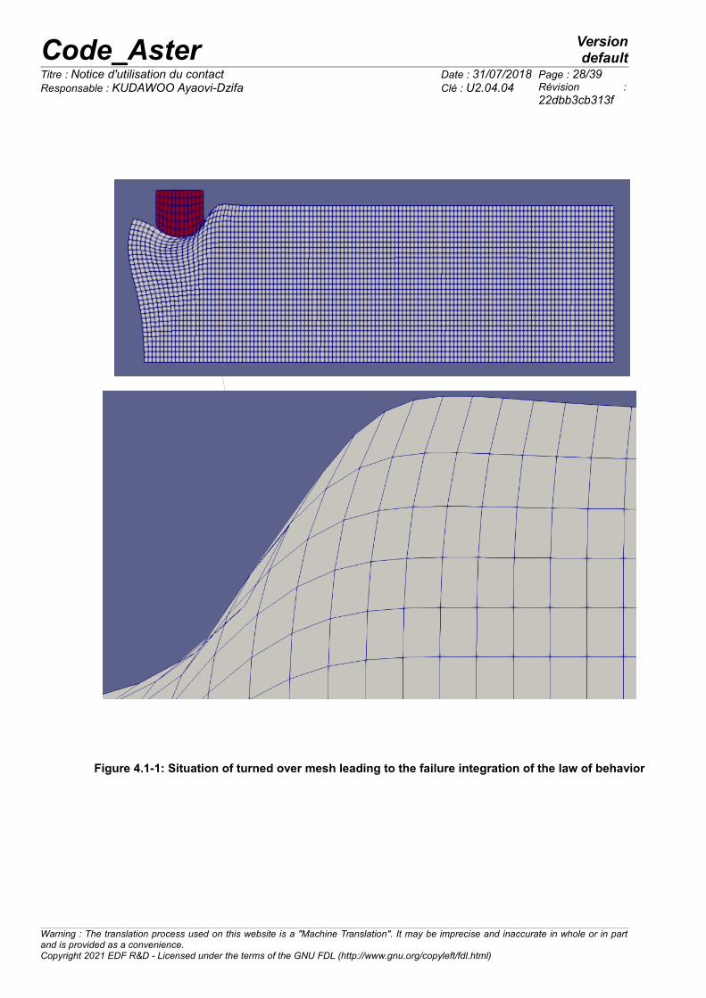
Code_Aster Versiondefault
Titre : Notice d'utilisation du contact Date : 31/07/2018 Page : 28/39Responsable : KUDAWOO Ayaovi-Dzifa Clé : U2.04.04 Révision :
22dbb3cb313f
Figure 4.1-1: Situation of turned over mesh leading to the failure integration of the law of behavior
Warning : The translation process used on this website is a "Machine Translation". It may be imprecise and inaccurate in whole or in partand is provided as a convenience.Copyright 2021 EDF R&D - Licensed under the terms of the GNU FDL (http://www.gnu.org/copyleft/fdl.html)
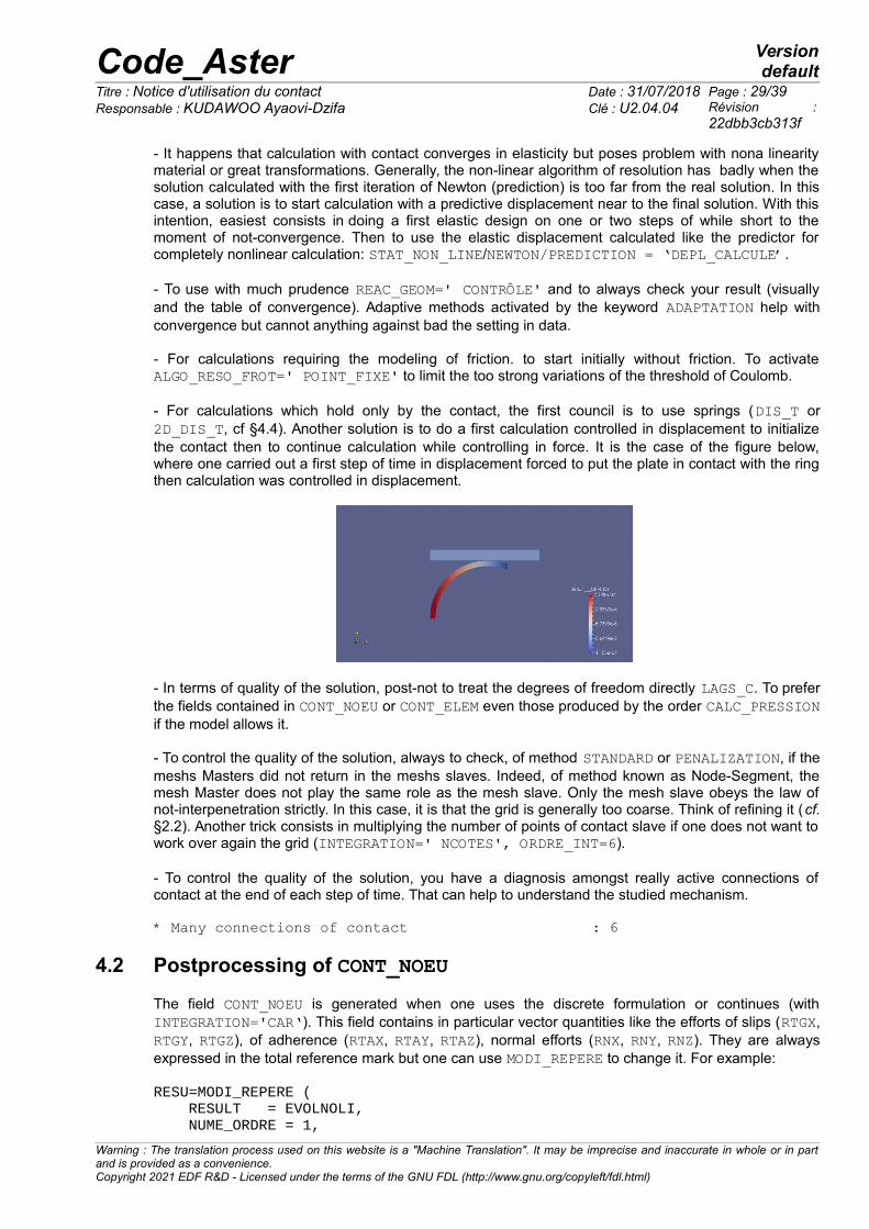
Code_Aster Versiondefault
Titre : Notice d'utilisation du contact Date : 31/07/2018 Page : 29/39Responsable : KUDAWOO Ayaovi-Dzifa Clé : U2.04.04 Révision :
22dbb3cb313f
- It happens that calculation with contact converges in elasticity but poses problem with nona linearitymaterial or great transformations. Generally, the non-linear algorithm of resolution has badly when thesolution calculated with the first iteration of Newton (prediction) is too far from the real solution. In thiscase, a solution is to start calculation with a predictive displacement near to the final solution. With thisintention, easiest consists in doing a first elastic design on one or two steps of while short to themoment of not-convergence. Then to use the elastic displacement calculated like the predictor forcompletely nonlinear calculation: STAT_NON_LINE/NEWTON/PREDICTION = ‘DEPL_CALCULE’.
- To use with much prudence REAC_GEOM=' CONTRÔLE' and to always check your result (visuallyand the table of convergence). Adaptive methods activated by the keyword ADAPTATION help withconvergence but cannot anything against bad the setting in data.
- For calculations requiring the modeling of friction. to start initially without friction. To activateALGO_RESO_FROT=' POINT_FIXE' to limit the too strong variations of the threshold of Coulomb.
- For calculations which hold only by the contact, the first council is to use springs (DIS_T or2D_DIS_T, cf §4.4). Another solution is to do a first calculation controlled in displacement to initializethe contact then to continue calculation while controlling in force. It is the case of the figure below,where one carried out a first step of time in displacement forced to put the plate in contact with the ringthen calculation was controlled in displacement.
- In terms of quality of the solution, post-not to treat the degrees of freedom directly LAGS_C. To preferthe fields contained in CONT_NOEU or CONT_ELEM even those produced by the order CALC_PRESSIONif the model allows it.
- To control the quality of the solution, always to check, of method STANDARD or PENALIZATION, if themeshs Masters did not return in the meshs slaves. Indeed, of method known as Node-Segment, themesh Master does not play the same role as the mesh slave. Only the mesh slave obeys the law ofnot-interpenetration strictly. In this case, it is that the grid is generally too coarse. Think of refining it (cf.§2.2). Another trick consists in multiplying the number of points of contact slave if one does not want towork over again the grid (INTEGRATION=' NCOTES', ORDRE_INT=6).
- To control the quality of the solution, you have a diagnosis amongst really active connections ofcontact at the end of each step of time. That can help to understand the studied mechanism.
* Many connections of contact : 6
4.2 Postprocessing of CONT_NOEU
The field CONT_NOEU is generated when one uses the discrete formulation or continues (withINTEGRATION='CAR‘). This field contains in particular vector quantities like the efforts of slips (RTGX,RTGY, RTGZ), of adherence (RTAX, RTAY, RTAZ), normal efforts (RNX, RNY, RNZ). They are alwaysexpressed in the total reference mark but one can use MODI_REPERE to change it. For example: RESU=MODI_REPERE ( RESULT = EVOLNOLI, NUME_ORDRE = 1,
Warning : The translation process used on this website is a "Machine Translation". It may be imprecise and inaccurate in whole or in partand is provided as a convenience.Copyright 2021 EDF R&D - Licensed under the terms of the GNU FDL (http://www.gnu.org/copyleft/fdl.html)
Code_Aster Versiondefault
Titre : Notice d'utilisation du contact Date : 31/07/2018 Page : 30/39Responsable : KUDAWOO Ayaovi-Dzifa Clé : U2.04.04 Révision :
22dbb3cb313f
MODI_CHAM = (_F (NOM_CHAM= ‘CONT_NOEU’, NOM_CMP = (‘RNX’, ‘RNY’, ‘RNZ’,), TYPE_CHAM= ‘VECT_3D’,),), REFERENCE MARK = ‘USER’, AFFE = _F (ANGL_NAUT= (45,45,0),),)
4.3 To recover the contact pressure 4.3.1 presentation of CALC_PRESSION
In postprocessing of a calculation of contact, one generally wishes to reach the efforts of contact-friction. More precisely, one wishes to know the normal and tangential constraint on the edge of thesolids in contact. The formulation continues contact gives access directly with an estimate of pressure of contact-friction,while the discrete formulations require to approximate it by the constraints on the edge.
An example of implementation for the two formulations exists in CAS-test SSNP154 [V6.03.154].CALC_PRESSION provides one CHAM_GD of printable contact pressure to the format counts forexample.
The contact pressure is written:
= .n .n (4)
where n is the normal on the surface of contact in deformed configuration and the tensor of theconstraints of Cauchy.
Framed below the watch how one can to calculate the nodal pressure of contact while usingCALC_PRESSION.
# calculation of the contact pressure: p_appr_Fp_appr_F=CALC_PRESSION (MAILLAGE=MESH, RESULTAT=RESU, GROUP_MA= (‘Bottom_C’, ‘Top_B’,), INST=1.0,);
For a calculation in great displacements, the normal must be calculated on the deformed configuration.For that it is necessary REnseigner the keyword GEOMETRIE=' DEFORMEE'.
In the example above, one uses the formula drawn from (4) to calculate the contact pressure explicitly.In the typical case where the edge on which one extracts the pressure is parallel to the axes of thereference mark, the pressure is directly equal to one of the diagonal components of the tensor of theconstraints of Cauchy (SIXX, SIYY or SIZZ). At present, one cannot use CALC_PRESSION if there areelements of structures in the model.
4.3.2 Case of Fcontinuous ormulation
In continuous formulation, the field DEPL contains one or more additional unknown factors:• LAGS_C represent the surface density the effort of contact expressed on the configuration
of reference.• LAGS_F1 and LAGS_F2 the coordinates of a directing vector in the tangent plan represent.
This vector of standard lower or equal to 1 indicates the direction of slip or adherencewhen which one takes into account friction.
Warning : The translation process used on this website is a "Machine Translation". It may be imprecise and inaccurate in whole or in partand is provided as a convenience.Copyright 2021 EDF R&D - Licensed under the terms of the GNU FDL (http://www.gnu.org/copyleft/fdl.html)
Code_Aster Versiondefault
Titre : Notice d'utilisation du contact Date : 31/07/2018 Page : 31/39Responsable : KUDAWOO Ayaovi-Dzifa Clé : U2.04.04 Révision :
22dbb3cb313f
These sizes are defined in any point of surface slave of contact. One can thus easily reach the contactpressure. One will however note that in great displacements, configuration initial and final beingconfused more, the degree of freedom LAGS_C any more the significance of a pressure does not have.
To reach the surface density the effort of friction (in phase of adherence like slip), should be carried outan additional calculation: the standard of the directing vector in the tangent plan indeed gives theamplitude compared to the threshold of friction.If one notes the contact pressure then density the effort of friction is written:
= . . LAGS F12 LAGS F22 (5)
In penalized formulation (ALGO_CONT=' PENALISATION'), the degrees of freedom of pressurecontinue to exist, one can thus apply what precedes. It happens sometimes that the contact pressure raised by this method present of the oscillations, inparticular for curved geometries. In this case, it is preferable to use CALC_PRESSION who calculatesthe contact pressure starting from the tensor of constraints of Cauchy.
4.3.3 Discrete formulation
In discrete formulation, no degree of freedom is added with the principal unknown factors. The problemof contact being formulated on the discrete system, the possible multipliers of Lagrange used do noteven have the dimension of a pressure but that of nodal forces.
This absence obliges to calculate the tensor of the constraints of Cauchy on the edge of surfaces incontact. There is only one alternative thus: CALC_PRESSION .
4.4 Movements of rigid bodies blocked by the contact
This paragraph applies only to the studies in statics. In dynamics, the movements of rigid body areallowed.
It arrives in the studies that the contact makes it possible to block the movements of rigid body ofcertain solids (and to make so that those become deformed). The initial not-catch in account of thisphenomenon will thus involve the singularity of the matrix of rigidity (and thus impossibility of solving).
The discrete formulations are not adapted to an initial taking into account of the contact, the realizationof studies with solids only held by the contact will thus require in this case an enrichment of modeling.The formulation continues makes it possible to take account of an initial contact naturally and for thisreason thus is well adapted under investigation mechanisms. For studies in three dimensions, there exist 6 movements of possible rigid bodies: 3 translations, 3rotations. For studies in two dimensions (modelings D_PLAN, C_PLAN), there exist 3 movements ofrigid body: 2 translations and a rotation. Axisymmetric modeling (AXIS) is particular: there exists onemovement of rigid body, the translation along the axis Oy (cylindrical axis of symmetry).
When one notes the existence of movements of rigid body in his modeling, one will always start bychecking that there do not exist symmetries in the structure and its loading . The conditions ofsymmetry indeed make it possible to remove most of the movements of rigid body.
An example of blocking of movements of rigid body in formulation continues (by CONTACT_INIT) andin discrete formulation (by springs) is available in CAS-test SSNA122 [V6.01.122].
4.4.1 Continuous formulation
Warning : The translation process used on this website is a "Machine Translation". It may be imprecise and inaccurate in whole or in partand is provided as a convenience.Copyright 2021 EDF R&D - Licensed under the terms of the GNU FDL (http://www.gnu.org/copyleft/fdl.html)

Code_Aster Versiondefault
Titre : Notice d'utilisation du contact Date : 31/07/2018 Page : 32/39Responsable : KUDAWOO Ayaovi-Dzifa Clé : U2.04.04 Révision :
22dbb3cb313f
In continuous formulation, the taking into account of an initial contact is assured zone by zone with thekeyword CONTACT_INIT. By defaults at the beginning of a calculation all the connections with nullgame (or interpenetrated) are activated (CONTACT_INIT=' INTERPENETRE'). The tolerance, to
determine if a game null or is interpenetrated, is fixed in-house in the program at 10−6×amin where
amin represent the smallest nonworthless edge of the grid. It is possible to disable this automatic activation (CONTACT_INIT=' NON'). When one does non-linearcalculations with recovery (i.e. with the keyword ETAT_INIT of STAT_NON_LINE), it is essential to usethe value by default (‘INTERPENETRATES’) in order to ensure a recovery starting from the true stateof contact (and not of a virgin state). Lastly, if one wants to stick initially all surfaces of contact independently of the initial game, one will beable to select CONTACT_INIT=' OUI' (that can be useful if the grids are not perfectly in contact).
In all the cases where an initial contact is declared, of the efforts will be generated: it is not about asimple geometrical repositioning aiming at sticking the grids.
The activation of an initial contact blocks the movements of rigid body following the normal direction tosurface. If one wants to take into account an initial adherent state in order to block the tangentdirection, one will be able to specify an initial threshold of contact not no one via SEUIL_INIT. Thisparameter informs the initial value of the contact pressure (homogeneous with a density of surfaceforce). By default, if calculation is resulting from a continuation then one automatically rebuilds thevalue of the initial threshold while using values of LAGS_C contents in ETAT_INIT/STAT_NON_LINE.
It should be noted that the use of an initial contact in continuous formulation as makes it possible to befreed from not-convergence when as a structure is subjected only to displacements. For example,when two solids initially in contact are in a hurry one against the other by displacements (it is thusabout a rigid movement of body).
4.4.2 Discrete formulation
In discrete formulation, one is obliged to manually block the movements of rigid body of the solidaccused by springs of low stiffness. By “weak” one understands sufficiently small to generate onlynegligible nodal forces in front of the nodal forces put concerned in calculation.The goal of the springs is to make so that calculation without contact is able to turn in linear mechanics(i.e. in the operator MECA_STATIQUE or in STAT_NON_LINE once withdrawn the conditions ofcontact). There exist two approaches for the addition of springs:
• to add a spring of low stiffness in any point of the structure• to add springs quite selected points to into cubes block the movements of rigid body of the
structure The first approach has the advantage of the generics but can disturb sometimes too much the solution(whatever the stiffness of the springs). Indeed such an approach amounts adding on all the diagonalterms of the matrix a positive term which makes it invertible.The second approach only adds springs where it is necessary. When there exist points of the structurewhich will be brought to have a weak displacement (thus not to generate that a weak nodal force in thespring), this approach is adapted more.
To apply a spring in Code_Aster, it is necessary to create meshs of the type POI1 starting from nodes.For that one uses the operator CREA_MAILLAGE/CRÉA_POI1. To use the first approach one willchoose to create this group of meshs on all the structure (TOUT=' OUI'), while for the secondapproach, one will indicate the group of nodes wished. The group of meshs lately created will be usedto affect a modeling of the type ‘DIS_T’ or ‘2D_DIS_T’ in AFFE_MODELE.
Warning : The translation process used on this website is a "Machine Translation". It may be imprecise and inaccurate in whole or in partand is provided as a convenience.Copyright 2021 EDF R&D - Licensed under the terms of the GNU FDL (http://www.gnu.org/copyleft/fdl.html)

Code_Aster Versiondefault
Titre : Notice d'utilisation du contact Date : 31/07/2018 Page : 33/39Responsable : KUDAWOO Ayaovi-Dzifa Clé : U2.04.04 Révision :
22dbb3cb313f
The definition of the characteristics of the spring is carried out in the operator AFFE_CARA_ELEM. Bydefaults, the stiffnesses entered the total reference mark. If for example one wishes to block a rigidmovement of body in a direction parallel with the axes of the total reference mark, one will define anonworthless stiffness only according to this direction. Below an example of definition of a stiffness fora calculation 2D according to the direction DY.
RESSORT=AFFE_CARA_ELEM (MODELE=model, DISCRET_2D=_F (CARA=' K_T_D_N', GROUP_MA=' SPRING', VALE= (0. , 1.0e-1,),),);
Whenever the direction to be blocked is not parallel to the axes, two alternatives are possible:• to define a stiffness according to all the directions• to define the stiffness in a local reference mark. It is then necessary to lay down the
direction of this reference mark (keyword ORIENTATION of AFFE_CARA_ELEM) or to usesprings being pressed either on meshs POI1 but SEG2.
For an example of use of springs, one will consult CAS-test ZZZZ237 and his documentation[V1.01.237].
4.5 Great deformations, great displacements and contact
The taking into account of conditions of contact-friction is completely uncoupled from the taking intoaccount of great displacements or great deformations. More generally, any non-linearity which is of anature material or geometrical is a priori compatible with the use of the contact.
In practice, one often notes difficulties of convergence in studies mixing three non-linearities. One givesin the continuation of this section the approach to be adopted in this case.
Examples of calculation mixing three non-linearities are available in CAS-tests SSNP155 [V6.03.155],SSNP157 [V6.03.157] and SDNV103 [V5.03.103].
For the method LAKE, it is possible to use TYPE_JACOBIEN=' ACTUALISE' instead of ‘INITIAL’in the case of great transformations.
4.5.1 To uncouple non-linearities
When that such a calculation fails, the first approach is to retrogress: by uncoupling non-linearities andwhile trying to apply the good practices into non-linear (cf. [U2.04.01]). That means:
• to carry out an elastic design in small disturbances with the activated contact. If thiscalculation fails, apply the advices delivered in the first part of this document (orientation ofthe normals, main choices of surfaces and slaves, choice of the algorithm of resolution,…)
• to carry out a calculation with a nonlinear law of behavior but without contact. If this onefails, then the problem comes from the integration of the behavior. One will refer then todocumentations [U2.04.02] and [U2.04.03].
• if necessary to carry out a calculation in great displacements but without contact and non-linearity material. If this calculation does not function, try to use another model amongthose of great displacements available in Code_Aster (‘SIMO_MIEHE’, ‘GDEF_LOG’,‘PETIT_REAC’).
4.5.2 To parameterize the algorithm of Newton well
If complete calculation (mixing all non-linearities) does not converge in spite of the application of thepreceding advices then one can try to exploit the parameters of the algorithm of Newton. That leavesthe following report:
Warning : The translation process used on this website is a "Machine Translation". It may be imprecise and inaccurate in whole or in partand is provided as a convenience.Copyright 2021 EDF R&D - Licensed under the terms of the GNU FDL (http://www.gnu.org/copyleft/fdl.html)

Code_Aster Versiondefault
Titre : Notice d'utilisation du contact Date : 31/07/2018 Page : 34/39Responsable : KUDAWOO Ayaovi-Dzifa Clé : U2.04.04 Révision :
22dbb3cb313f
When one couples contact and non-linearity material for example, it is possible (by the“abrupt” correction of the contact) to start in the law of behavior of the mechanisms (left the elasticrange, discharges) which should not be active in the final solution and which are likely to degrade thetangent matrix (until making it noninvertible). That makes then any convergence impossible.
One thus proposes to use the following adjustments in the algorithm of Newton (operatorSTAT_NON_LINE or DYNA_NON_LINE):
• reactualization of the tangent matrix to each iteration (REAC_ITER=1)• use of an elastic prediction (PREDICTION=' ELASTIQUE')• in great deformations (DEFORMATION= ' SIMO_MIEHE'), the tangent matrix is
nonsymmetrical, it is thus necessary well to take care to inform SYME=' NON' in thekeyword SOLVEUR.
When calculation has still difficulty converging, it is necessary to return to modeling:
• does my calculation cause problems of incompressibility? In this case, consultdocumentations [U2.04.01] [U2.04.02] and try to use adapted finite elements (under-integrated, with mixed formulation).
• the behavior that I use have a coherent tangent matrix? If it is not the case, one can try asa last resort to use a matrix ‘ELASTIC’ and to increase the iteration count of Newton.
• Case plasticité+contact+grandes transformations: if the initial solution is far from thesolution sought then Newton fails. In certain cases, it can be necessary to do a firstpredictive calculation (contact replaced for example by LIAISON_MAIL ) then to inject theresult resulting from this predictive calculation in the calculation which one wishes to carryout.
• To privilege the mode all PENALIZATION by regulating the authorized maximumpenetration is also an alternative: PENE_MAXI.
4.5.3 Resolution of a quasi-static problem in slow dynamics
As a last resort, for the quasi-static problems, to carry out a dynamic calculation in long time can bringa solution. The matrix of mass causes to stabilize the structure, it should however be made sure thatthe inertial forces remain weak then in front of the internal forces of the system.
One advises for this kind of modeling to assign to the structure his true density (it is obligatory in anycase in the presence of loading of gravity) and to carry out calculation by using great steps of time.
An example of implementation is available in CAS-test SSNP155 [V6.03.155].
4.6 Rigid surface and contact
Sometimes one wishes to model in the studies of the rigid solids which make contact with deformablesolids. In this section, it is explained how to optimize such studies.
In order not to weigh down modeling the rigid solids will not be entirely modelled: only their edge willcarry degrees of freedom. In order to facilitate the orientation of the normals of this rigid solid the gridwill comprise the complete solid however.
After having directed the normals, one will thus affect in AFFE_MODELE only elements of edge to theskin of the rigid solid: as the elements of edge do not carry rigidity, an alarm is emitted to prevent risk ofnoninvertible matrix of rigidity. This alarm is normal in this case and can be been unaware of. To prevent that the matrix of rigidity is singular, it is necessary to impose the displacement of all thedegrees of freedom carried by the rigid edge. That is done with the orders:
• AFFE_CHAR_CINE/MECA_IMPO from which the advantage is to eliminate the unknownfactors
• AFFE_CHAR_MECA/DDL_IMPO who adds additional unknown factors to the problem.•
Warning : The translation process used on this website is a "Machine Translation". It may be imprecise and inaccurate in whole or in partand is provided as a convenience.Copyright 2021 EDF R&D - Licensed under the terms of the GNU FDL (http://www.gnu.org/copyleft/fdl.html)

Code_Aster Versiondefault
Titre : Notice d'utilisation du contact Date : 31/07/2018 Page : 35/39Responsable : KUDAWOO Ayaovi-Dzifa Clé : U2.04.04 Révision :
22dbb3cb313f
One thus advises to eliminate the unknown factors (AFFE_CHAR_CINE).
Rigid surface will be declared like surface Master in DEFI_CONTACT as explained with the §2.2.1. One will be able to refer to CAS-test SSNV506 [V6.04.506] for an example of contact with rigid surface.
4.7 Redundancy between conditions of contact-friction and boundaryconditions (symmetry): methods other than LAKE
In the presence of symmetries in the studied structure, it is current that the conditions of friction enter inconflict with the boundary conditions of symmetry. Figure 4.7-1 watch the example of two cubes incontact-friction, the hatched part represents the faces of the cubes subjected to a condition ofsymmetry (DX=0).In this example, the edge of the higher cube in thick feature belongs to surface slave and also carriesthe condition of symmetry. This condition enters in conflict with the condition of friction written thetangent plan (here the plan xOz ). In practice calculation will once stop the established contactbecause the tangent matrix will be singular.Mechanically it is seen that the condition of symmetry implies that adherence or the slip will occur onlyaccording to the direction DZ (green tangent vector). To eliminate the redundancy it is thus necessaryto exclude the direction from following friction DX (red tangent vector).
For that one will use the keyword SANS_GROUP_NO_FR to indicate the list of nodes of the edge slavethen one will inform (in the total reference mark) DIRE_EXCL_FROT= (1,0,0) that is to say directionDX to exclude.
CAS-test ZZZZ292 implements the functionality SANS_GROUP_NO_FR.
Warning : The translation process used on this website is a "Machine Translation". It may be imprecise and inaccurate in whole or in partand is provided as a convenience.Copyright 2021 EDF R&D - Licensed under the terms of the GNU FDL (http://www.gnu.org/copyleft/fdl.html)

Code_Aster Versiondefault
Titre : Notice d'utilisation du contact Date : 31/07/2018 Page : 36/39Responsable : KUDAWOO Ayaovi-Dzifa Clé : U2.04.04 Révision :
22dbb3cb313f
Figure 4.7-1: Elimination of directions of friction
4.8 To measure the interpenetration without solving the contact:methods other than LAKE
The resolution of a problem of contact sometimes which can be expensive it can be advantageous toreplace the imposition of the conditions of contact by a simple checking of the interpenetration. It is allthe more interesting whenever one simply wishes to check that solids will not make contact.For each zone of contact defined in the operator DEFI_CONTACT, it is possible to choose if one wishesto enforce the contact there (RESOLUTION=' OUI') or not (RESOLUTION=' NON'). The interest of such an approach is not to weigh down a calculation: when that a calculation carried outwithout resolution on the entirety of the zones of contact watch that there is no interpenetration thenone can be unaware of the modeling of the contact.Attention however: so at least one of the zones of contact “is solved” and the another “unsolved” thenexistence of an interpenetration does not prejudge a solution of a complete calculation with contact(because of possible interactions between zones of contact).
Finally this technique can be also used to measure the rate of interpenetration on the level of the zonesof contact to gauge a criterion like the coefficient of penalization or the maximum interpenetrationtolerated in the method of resolution ‘GCP’ .
4.9 To display the results of a calculation of contact
Warning : The translation process used on this website is a "Machine Translation". It may be imprecise and inaccurate in whole or in partand is provided as a convenience.Copyright 2021 EDF R&D - Licensed under the terms of the GNU FDL (http://www.gnu.org/copyleft/fdl.html)
slave
Master
X
there
Z
Code_Aster Versiondefault
Titre : Notice d'utilisation du contact Date : 31/07/2018 Page : 37/39Responsable : KUDAWOO Ayaovi-Dzifa Clé : U2.04.04 Révision :
22dbb3cb313f
When one displays the results of a calculation of contact-friction in a software of postprocessing, it isnecessary to take care of several things:
• for the posting of the deformations, a factor of amplification different from 1 can resultin visualizing nonreal interpenetrations
• for calculations 2D in formulation ‘CONTINUES’, one will pay attention during the postingof deformations to the software of postprocessing which regards the first threecomponents of a field as the components according to X , Y and Z displacement. In2D, the third component corresponds to LAGS_C and must thus be been unaware of
• case standard/penalized method: during the visualization of the field of postprocessing ofthe contact (CONT_NOEU) and more particularly of the component CONT who indicates thestate of the contact, one will sometimes automatically pay attention to the interpolation ofthe fields to the nodes realized. Indeed this component takes values 0 (not contact), 1(adherent contact) or 2 (slipping contact). The adherent state is not possible that in thepresence of friction: if one visualizes such a value for a calculation of contact withoutfriction it is that there is interpolation of the field.
• Case method LAKE: the field CONT_ELEM is provided in postprocessing. The componentsare described in detail in Doc. U4.44.11 page 34 .
4.10 Specific contact with discrete elements (springs)
Discrete elements (or springs) 2D_DIS_T* or DIS_T* associated with the law of behavior DIS_CHOC[R5.03.17] allow to give an account of a specific contact in a fixed direction. They are well adapted tothe modeling of shocks and for this reason are often used in dynamics on modal basis [U4.53.21] andin explicit dynamics [U4.53.01].The springs can be based indifferently on a specific mesh or a segment. In all the cases, it isnecessary to correctly direct each element with the order AFFE_CARA_ELEM [U4.42.01].The contact as friction are solved by penalization (cf §3.2.2). The stiffnesses of penalization, thecoefficient of friction as well as the initial games are specified in material DIS_CONTACT (orderDEFI_MATERIAU, [U4.43.01]).
This kind of element is not usable in great displacements because the direction of contact fixed and isgiven by the initial orientation of the discrete element.
CAS-tests SSNL130A and SDND100C implement springs of contact.
4.11 Elements of joints (hydro) mechanical with contact and friction
Elements of joints (hydro) mechanical PLAN_JOINT (_HYME) and 3D_JOINT (_HYME) allow tomodel the opening of a crack under the pressure of a fluid and friction on the edges of the crack closedwith the law JOINT_MECA_FROT [R7.01.25]. It is possible to couple the opening of the crack and thepropagation of the fluid with modelings *_HYME.The formulation of contact-friction is penalized and the related parameters are indicated under thekeyword JOINT_MECA_FROT order DEFI_MATERIAU [U4.43.01].
CAS-tests SSNP142C and SSNP142D provide an example of application of such elements on themodeling of a stopping.
4.12 Use of the adaptive methods
Case 1 : The statutes have difficulty being stabilized in continuous formulation (all algorithms), to useADAPTATION=' CYCLAGE' .
Case 2 : ALGO_CONT=' STANDARD' fail and I want to use the mode PENALIZATION but I do notknow how to regulate the coefficient of penalization, to use the mode ALGO_CONT=' PENALISATION'and ADAPTATION=' ADAPT_COEF'. By default, there is a keyword which is activated PENE_MAXI
Warning : The translation process used on this website is a "Machine Translation". It may be imprecise and inaccurate in whole or in partand is provided as a convenience.Copyright 2021 EDF R&D - Licensed under the terms of the GNU FDL (http://www.gnu.org/copyleft/fdl.html)

Code_Aster Versiondefault
Titre : Notice d'utilisation du contact Date : 31/07/2018 Page : 38/39Responsable : KUDAWOO Ayaovi-Dzifa Clé : U2.04.04 Révision :
22dbb3cb313f
who is equal to 1.E-2 time the smallest edge of mesh in the zone of contact. PENE_MAXI can berather easily estimated by the user because it is directly connected corresponding to a mesh of contact.
Case 3 : if case 2 fails to use ADAPTATION='ALL‘. Other cases : if one uses the formulation continues and ALGO_CONT='STANDARD'/‘PENALIZATION’ then prear defect method of adaptation ‘CYCLING’ is active. Oneadvises, if convergence allows it, to use automatic reactualization geometrical REAC_GEOM='AUTOMATIQUE' (parameter setting by default).
Warning : The translation process used on this website is a "Machine Translation". It may be imprecise and inaccurate in whole or in partand is provided as a convenience.Copyright 2021 EDF R&D - Licensed under the terms of the GNU FDL (http://www.gnu.org/copyleft/fdl.html)

Code_Aster Versiondefault
Titre : Notice d'utilisation du contact Date : 31/07/2018 Page : 39/39Responsable : KUDAWOO Ayaovi-Dzifa Clé : U2.04.04 Révision :
22dbb3cb313f
5 Bibliography
[1] MR. ABBAS. “Discrete formulation of contact-friction”. Reference material of Code_Aster.[R5.03.50].
[2] MR. ABBAS. “Elements of contact derived from a continuous hybrid formulation”. Referencematerial of Code_Aster. [R5.03.52].
[3] T. SOZA. “Operator DEFI_CONTACT ”. Documentation of use of Code_Aster. [U4.44.11].
[4] A. KONTER. “Advanced Finite Element Benchmarks Contact”. NAFEMS, 2006.
[5] A. KONTER. “How to undertake has contact and friction analysis”. NAFEMS, 2000.
Warning : The translation process used on this website is a "Machine Translation". It may be imprecise and inaccurate in whole or in partand is provided as a convenience.Copyright 2021 EDF R&D - Licensed under the terms of the GNU FDL (http://www.gnu.org/copyleft/fdl.html)