north slope portable oil and gas operation simulation
TRANSCRIPT

Prepared by: AECOM
October 17, 2017
WORKGROUP FOR GLOBAL AIR PERMIT POLICY DEVELOPMENT
FOR TEMPORARY OIL AND GAS DRILL RIGS
Technical Subgroup
Ambient Demonstration
for the
North Slope Portable Oil and Gas Operation Simulation
FINAL

Workgroup for Global Air Permit Policy Development for Temporary Oil and Gas Drill Rigs October 17, 2017
North Slope POGO Simulation
Page 2 of 54
TABLE OF CONTENTS
1. INTRODUCTION................................................................................................................. 7
1.1 Background Information Regarding the Workgroup ....................................................... 7
1.2 Modeling Analysis Summary ........................................................................................... 8
2. BACKGROUND ................................................................................................................... 9
2.1 Project Location and Description ..................................................................................... 9
2.2 Project Classification...................................................................................................... 12
2.3 Modeling Protocol Submittal ......................................................................................... 12
3. SOURCE IMPACT ANALYSIS ....................................................................................... 12
3.1 Modeling Approach........................................................................................................ 13
3.2 Model Selection.............................................................................................................. 16
3.3 Meteorological Data ....................................................................................................... 16
3.4 Coordinate System ......................................................................................................... 17
3.5 EU Inventory .................................................................................................................. 17
3.6 Non-Modeled EUs.......................................................................................................... 18
3.7 EU Release Parameters .................................................................................................. 23
3.7.1 Emission Rates ........................................................................................................ 23
3.7.1.1 Sulfur Compound Emissions ............................................................................. 23
3.7.1.2 Operational Limits ............................................................................................ 23
3.7.1.3 Short-Term Emission Rates............................................................................... 23
3.7.1.4 Application of Temporally-Varying Emissions ................................................. 24
3.7.2 Point Source Parameters ........................................................................................ 25
3.8 Pollutant-Specific Considerations .................................................................................. 31
3.8.1 Ambient NO2 Modeling ........................................................................................... 31
3.8.1.1 USEPA and ADEC Approval ............................................................................ 31
3.8.1.2 Public Comment ................................................................................................ 31
3.8.1.3 In-Stack NO2-to-NOX Ratio ............................................................................... 31
3.8.1.4 Ozone Data ....................................................................................................... 33
3.8.2 Qualitative Assessment of Secondary PM2.5 Impacts.............................................. 33
3.9 Downwash ...................................................................................................................... 35
3.10 Ambient Air Boundary ................................................................................................... 35
3.11 Receptor Grid ................................................................................................................. 36
Workgroup for Global Air Permit Policy Development for Temporary Oil and Gas Drill Rigs October 17, 2017
North Slope POGO Simulation
Page 3 of 54
3.12 Off-Site Source Impacts and Characterization ............................................................... 36
3.13 Ambient Background Concentrations ............................................................................ 38
3.13.1 A-Pad Ambient Air and Meteorological Monitoring Station .................................. 41
3.13.2 CD1 Ambient Air and Meteorological Monitoring Station .................................... 46
3.14 Design Concentrations ................................................................................................... 47
3.15 Post-Processing .............................................................................................................. 47
4. RESULTS AND DISCUSSION ......................................................................................... 49
4.1 Conservatism in the Modeling Demonstration............................................................... 49
5. CONCLUSIONS ................................................................................................................. 53
5.1 Summary of Key Parameters and Assumptions ............................................................. 53
5.2 Summary of Conclusions ............................................................................................... 54
TABLE OF APPENDICES
APPENDIX A AERMOD Sensitivity Analyses
APPENDIX B Drill Rig Equipment Inventory Survey
APPENDIX C Transportable Source Variability Processor (TRANSVAP)
APPENDIX D Second Tier Approach to Combining Model-Predicted Impacts with a
Monitored NO2 Background Concentration
APPENDIX E Hydraulic Fracturing in Alaska

Workgroup for Global Air Permit Policy Development for Temporary Oil and Gas Drill Rigs October 17, 2017
North Slope POGO Simulation
Page 4 of 54
TABLE OF TABLES
Table 1 POGO Categories............................................................................................................ 8
Table 2 Maximum Modeled Quantity of Fuel That a North Slope POGO Could Consume
Without Violating an AAAQS (Gallons per Day) .......................................................... 9
Table 3 Modeled EU Inventory ................................................................................................. 19
Table 4 Example Non-Modeled EUs ......................................................................................... 22
Table 5 Base Emission Rates (Grams per Second) for a Drill Rig Operating at 10,000
Gallons per Day ............................................................................................................ 26
Table 6 Nominal Emissions Scaling Factor Used as Input to AERMOD ................................. 26
Table 7 Stack Parameters during Nominal Operation ............................................................... 28
Table 8 Stack Parameters during Excursions from Nominal Operation .................................... 29
Table 9 Location of Emission Releases at Each Drilling Location (Plant Coordinates) ........... 30
Table 10 Summary of the Background Concentrations Used in the North Slope POGO
Simulation ..................................................................................................................... 39
Table 11 Summary of Direct Representativeness of Four North Slope Datasets ........................ 43
Table 12 Allowed Design Concentrations and Applicable AAAQS and NAAQS...................... 48
Table 13 Summary of Results ...................................................................................................... 52
Table 14 Maximum Modeled Quantity of Fuel That a North Slope POGO Could Consume
Without Violating an AAAQS (Gallons per Day) ........................................................ 54

Workgroup for Global Air Permit Policy Development for Temporary Oil and Gas Drill Rigs October 17, 2017
North Slope POGO Simulation
Page 5 of 54
TABLE OF FIGURES
Figure 1 Alaskan North Slope ..................................................................................................... 11
Figure 2 Generalized Approach for Determining the Maximum Daily Fuel Consumption ....... 14
Figure 3 Placement of the Emissions Units on the Representative Modeled Drill Rig ............. 20
Figure 4 Configuration of the Representative Well Pad with Five Modeled Well
(Drill Rig) Locations ..................................................................................................... 21
Figure 5 Normalized 1-hour NO2 Seasonally-Varying Emission Rates with Transient Hourly
Excursions for (a) Heaters and Boilers and (b) Engines for a Typical Year ................ 27
Figure 6 Full AERMOD Receptor Grid ...................................................................................... 37
Figure 7 Meteorological and Ambient Air Monitoring Stations Used for the North Slope
POGO Simulation ......................................................................................................... 40
Figure 8 Comparison of A-Pad Ambient Data and Drill Rig Activity Onsite ............................ 45
Figure 9 Visualization of the Frequency of an Actual Hydraulic Fracturing Operation
at the CD1 Pad .............................................................................................................. 46
Figure 10 (a) 1-hour NO2 and (b) 1-hour SO2 Model-Predicted Impacts after TRANSVAP
Post-Processing ............................................................................................................. 51
lltorirymrry &r Globsl *{ir Pcmit Feticy Devcl*prnont &r Trmporary Oil md ffas I}rffi nigs Ot*obEr I ?, 301 7Itlsfih Slope fCIG$ Simulstisn
This report was rcyiswsd and appr*ved by tlre Terhniffil $xbgmr:p ruf the trHorkgroup for ffIcbslAir Pcrrnit Pelicy Developrasnt for ?empunry Sil rnd fr*$ ftitl Rigs. ?he f*llowing r*embcrs oftfte Twhnical Subgroup signed thr reprt on beh*lf af their affilistion:
Brad Ttrsrnss
ConomPhillips
Alaska S*pfqlri
lnu.
Allian*r
Aleskr 6il *nd Gac Assoclati$t!
AIfin E. Sckulcr, F.E,
Alasks ileparttneat af E$virqfl rnu*tal C$fissrynticn
Fagr 6 of54
?4Dr?

Workgroup for Global Air Permit Policy Development for Temporary Oil and Gas Drill Rigs October 17, 2017
North Slope POGO Simulation
Page 7 of 54
1. INTRODUCTION
This report was prepared by the Technical Subgroup of the Workgroup for Global Air Permit
Policy Development for Temporary Oil and Gas Drill Rigs (Workgroup). This report describes
the air quality modeling approach and assumptions used for assessing air quality impacts from
North Slope portable oil and gas operations (POGOs).1 The analysis demonstrates that operating a
North Slope POGO within the constraints described in this report will not cause or contribute to a
violation of the following Alaska Ambient Air Quality Standards (AAAQS) listed in
18 AAC 50.010:2
Sulfur dioxide (SO2): 1-hour, 3-hour, 24-hour, and annual averaging periods.
Carbon monoxide (CO): 1-hour and 8-hour averaging periods.
Nitrogen dioxide (NO2): 1-hour and annual averaging periods.
Particulate matter having an aerodynamic diameter of 10 microns or less (PM10): 24-hour
averaging period.
Particulate matter having an aerodynamic diameter of 2.5 microns or less (PM2.5): 24-hour
and annual averaging periods.
1.1 Background Information Regarding the Workgroup
The Workgroup was organized to develop recommendations for streamlining the air
permitting process for POGOs within the State of Alaska.3 The Workgroup consists of
representatives from the following interested parties:
Alaska Department of Environmental Conservation (ADEC), Division of Air Quality.
Alaska Department of Natural Resources (ADNR), Division of Oil and Gas.
Alaska Oil and Gas Association (AOGA).
Cook Inlet Regional Citizens Advisory Council (CIRCAC).
Alaska Support Industry Alliance (ASIA).
North Slope Borough (NSB).
The Workgroup created and engaged the Technical Subgroup to address the technical issues
associated with the Workgroup’s goals. The Workgroup also created a Policy Subgroup to
address regulatory and policy matters. This report only addresses an air quality modeling
1 A “Portable Oil and Gas Operation” (POGO) under 18 Alaska Administrative Code (AAC) 50.990(124) means
“an operation that moves from site to site to drill or test one or more oil or gas wells, and that uses drill rigs,
equipment associated with drill rigs and drill operations, well test flares, equipment associated with well test
flares, camps or equipment associated with camps; ‘portable oil and gas operation’ does not includes well
servicing activities; for the purposes of this paragraph, ‘test’ means a test that involves the use of a flare.” 2 The listed AAAQS are identical to the National Ambient Air Quality Standards (NAAQS) set forth in Title 40 of
the Code of Federal Regulations, Part 50 (40 CFR 50). 3
Additional information on the Workgroup for Global Air Permit Policy Development for Temporary Oil and Gas
Drill Rigs and associated subgroups can be found on the Workgroup website
(http://dec.alaska.gov/air/ap/OilGasDrillWorkgroup.html).

Workgroup for Global Air Permit Policy Development for Temporary Oil and Gas Drill Rigs October 17, 2017
North Slope POGO Simulation
Page 8 of 54
assessment conducted for North Slope POGOs by the Technical Subgroup. Regulatory and
policy matters associated with these findings are not directly addressed in this report.
1.2 Modeling Analysis Summary
The Technical Subgroup developed a quantitative modeling approach for assessing four
categories of onshore POGO activity that typically occur on the Alaskan North Slope. These
four POGO categories are described in Table 1. Using the techniques described in this
modeling report, the Technical Subgroup developed a generic North Slope POGO simulation
(North Slope POGO Simulation) for each category that represent drill rig operations powered
by liquid-fired reciprocating internal combustion engines (RICE) and other support
equipment and activities.4 Based on the results of the modeling analysis, the Technical
Subgroup concluded that North Slope POGOs could consume up to the fuel levels shown in
Table 2 without causing or contributing to a violation of the AAAQS.
Table 1 POGO Categories
POGO
Category Description
RDi
Routine Infill Drilling at an Isolated Well Pad: Onshore drilling that lasts less than
24 consecutive months at a well pad that is not adjacent to, adjoining, or abutting a
major stationary source.
RDc
Routine Infill Drilling at a Collocated Well Pad: Onshore drilling that lasts less than
24 consecutive months at a well pad that is adjacent to, adjoining, or abutting a major
stationary source.
DDi
Developmental Drilling at an Isolated Well Pad: Onshore drilling that lasts greater
than 24 consecutive months at a well pad that is not adjacent to, adjoining, or abutting a
major stationary source.
DDc
Developmental Drilling at a Collocated Well Pad: Onshore drilling that lasts greater
than 24 consecutive months at a well pad that is adjacent to, adjoining, or abutting a
major stationary source.
4 The Technical Subgroup did not evaluate drilling operations powered by gas-fired or dual fuel-fired RICE EUs
or gas/liquid-fired combustion turbines.

Workgroup for Global Air Permit Policy Development for Temporary Oil and Gas Drill Rigs October 17, 2017
North Slope POGO Simulation
Page 9 of 54
Table 2 Maximumb Modeled Quantity of Fuel That a North Slope POGO
a Could Consume
Without Violating an AAAQS (Gallons per Day)
Allowable Onshore Drill Rig Operation RDi b RDc
b DDi
b DDc
b
POGO Without Concurrent Hydraulic Fracturing Activities c 14,700 11,400 14,700 10,700
POGO With Concurrent Hydraulic Fracturing Activities c 11,400 11,400 10,700 10,700
a Daily fuel consumption thresholds apply to the drill rig only and do not apply to other emissions units that
may be a part of the POGO or operating on the well pad, such as stationary well pad equipment, portable
power generators, or well servicing equipment (as defined in 18 AAC 50.990(125)) – these activities are
represented by the background values added to the modeled impacts. An example list of this equipment is
outlined in Table 4. b Daily fuel consumption thresholds can be exceeded by 25 percent, 20 percent of the days in a year (73 days
per year), which is equivalent to the following daily volumes:
14,700 x 1.25 = 18,375 gallons per day.
11,400 x 1.25 = 14,250 gallons per day.
10,700 x 1.25 = 13,375 gallons per day. c Hydraulic fracturing in Alaska is discussed in Appendix E.
2. BACKGROUND
The following subsections provide additional background on the development of the North Slope
POGO Simulation.
2.1 Project Location and Description
Drill rigs have been operating on the North Slope of Alaska since the 1940’s but did not have
a continuous presence until the mid-1960’s when an economically viable oil pool was first
discovered at Prudhoe Bay in 1967. The Technical Subgroup reviewed POGOs operating on
the North Slope for the last decade to develop a dispersion modeling simulation for this
analysis.
POGOs consist of equipment associated with drill rigs and drilling operations, well test
flares, camps, and equipment associated with camps. This equipment is typically owned and
operated by contractors working for North Slope Operators and not the operators themselves.
Equipment associated with a drill rig consists of the primary drilling engines, large and small
utility engines, and heaters and boilers. The primary drilling and large utility engines are
typically large engines ranging from approximately 600 brake-horsepower (bhp) to 2,200 bhp
each. The small utility engines are typically less than 600 bhp, and the heaters and boilers are
typically less than 10 million British thermal units per hour (MMBtu/hr) each. Equipment
associated with camps typically include portable power generators rated from between 400 to
750 kilowatts-electric (kWe). POGOs are also often accompanied by an array of small
portable engines and heaters and other mobile equipment supporting the operation, such as
trucks, light plants, welders, construction equipment, and/or snow removal equipment.
However, these types of equipment only operate intermittently and do not accompany a
Workgroup for Global Air Permit Policy Development for Temporary Oil and Gas Drill Rigs October 17, 2017
North Slope POGO Simulation
Page 10 of 54
POGO at all times. Portable flares may accompany POGOs on the North Slope and are used
when there is either a lack of infrastructure in place to capture excess gas or in emergency
upset conditions.
POGOs can move from one site to another to drill new wells. A site may be either gravel
well pads with year-round access or temporary ice pads used to drill exploration wells. The
amount of time a POGO is located at a particular site can vary from as short as a month or
less when drilling single wells to as long as several years for sustained development drilling.
On average, a particular POGO is at a North Slope well pad for approximately
30 consecutive days.5 Typically, a well pad will be devoid of a POGO for approximately
160 days in the case of infill drilling.5 However, depending on the pad it can be years, before
a POGO returns to a well pad. In the case of developmental drilling, a particular POGO may
also move from one location to another while at a well pad and it may do this for an extended
period of time. However, even in this case, a drill rig will not generally operate at a single
location for more than 30 to 60 days.
At any given time, there are likely multiple POGOs on the North Slope. Based on data
collected from 1990 to 2012, there are typically less than 10 drill rigs engaged in drilling
wells across the entire State of Alaska during any given week of the year. This stands in stark
contrast to the number of active drilling rigs nationwide, which have numbered in the
thousands over the same time period.
Equipment associated with POGOs are powered by either (1) burning a liquid fuel, (2)
burning a gaseous fuel, (3) electrically, or “highline” power, from an off-site source, or (4) a
combination of all of these. Small, intermittently-used, and/or emergency equipment
typically burn liquid fuel, while the power source for other larger equipment may vary based
on location and availability. Due to cost considerations, however, highline electricity is often
the preferred source of power for these operations whenever available. When equipment
burns a liquid fuel, nonroad engines are required to burn Ultra-Low Sulfur Diesel (ULSD)
under Federal regulations. ULSD has a maximum sulfur content of 0.0015 percent by weight.
There are no similar Federal requirements for heaters and boilers, therefore, North Slope
operators typically operate these emissions units (EUs) on either ULSD or an Arctic grade
fuel called Low End Point Diesel (LEPD). LEPD has a maximum sulfur content of 0.15
percent by weight. Similar to highline, the use of LEPD varies based on location and
availability.
The aforementioned characteristics of POGOs are generally applicable to all onshore
operations across the North Slope. The North Slope of Alaska is generally considered to
range from the Brooks Range Mountains, extending north to the Beaufort Sea and west to the
Chukchi Sea. For the purposes of this report, the North Slope is approximately defined as
north of 69 degrees, 30 minutes North latitude in the State of Alaska, consistent with the
definition in ADEC’s Minor General Permit 1 (MG1). Figure 1 illustrates the approximate
coverage area.
5
Average activity and inactivity at typical North Slope well pads is discussed in Appendix C.

Workgroup for Global Air Permit Policy Development for Temporary Oil and Gas Drill Rigs October 17, 2017
North Slope POGO Simulation
Page 11 of 54
Figure 1 Alaskan North Slope

Workgroup for Global Air Permit Policy Development for Temporary Oil and Gas Drill Rigs October 17, 2017
North Slope POGO Simulation
Page 12 of 54
2.2 Project Classification
The Technical Subgroup assumed that the North Slope POGOs under consideration would
only be subject to minor source New Source Review (NSR), rather than Prevention of
Significant Deterioration (PSD) review. Therefore, this modeling demonstration for the
North Slope POGO Simulation was prepared to satisfy ambient air quality demonstration
requirements under Alaska’s minor source permitting program in 18 AAC 50.502. With this
objective in mind, the Technical Subgroup compared the simulated impacts to just the
AAAQS, rather than the AAAQS and PSD increments.6 However, the Technical Subgroup
went beyond the requirements in 18 AAC 50.502 by assessing compliance with all
applicable AAAQS, rather than only the AAAQS triggered by a POGO minor permit
classification under 18 AAC 50.502(c)(2)(A).
2.3 Modeling Protocol Submittal
The Technical Subgroup did not develop a modeling protocol for the North Slope POGO
Simulation because all approaches and methods were developed collaboratively with ADEC
throughout the modeling process.
3. SOURCE IMPACT ANALYSIS
The Technical Subgroup used a computer analysis (modeling) to predict the ambient air quality
impacts for the pollutants outlined in the Introduction of this report. A modeling analysis for lead
(Pb), ammonia (NH3), or secondary pollutants, including ozone (O3) and secondary PM2.5, was
not conducted.
Lead is not a concern because it is not an additive in fuels used in North Slope POGOs. Lead
would only be present at trace element levels as a result of engine lubricant constituents or as a
result of engine wear and is negligible. Therefore, lead emissions from equipment associated
with POGOs will be negligible and would not cause or contribute to an exceedance of the lead
AAAQS.
Ammonia is not emitted by equipment or activities associated with POGOs, and concentrations
have been shown to be low on the North Slope. Therefore, ammonia is not a concern.
Although O3 is a criteria pollutant, it is not emitted directly into the atmosphere but rather
formed by chemical reactions of precursor pollutants, primarily nitrogen oxides (NOX) and
volatile organic compounds (VOCs). Based on current regional air quality monitoring data (i.e.
measured ground-level O3 concentrations are well below the AAAQS) and the low magnitude of
POGO emissions of precursors compared to the total precursor loading in the air shed, POGOs
are not expected to have a significant impact on ambient O3 generation on the North Slope. No
evidence exists to suggest net O3 production on the North Slope, but evidence does suggest
scavenging, i.e. ozone decrease due to chemical reactions.
6
The PSD Increment was also discussed at the Tenth Meeting of the Workgroup on February 4, 2016. Meeting
minutes and transcript are available on the Workgroup website
(http://dec.alaska.gov/air/ap/OilGasWorkgroup.html).

Workgroup for Global Air Permit Policy Development for Temporary Oil and Gas Drill Rigs October 17, 2017
North Slope POGO Simulation
Page 13 of 54
3.1 Modeling Approach
The North Slope POGO Simulation was designed to quantitatively assess air quality impacts
using dispersion modeling for any POGO on the North Slope. Explicit modeling focused on
that portion of the POGO that remains stationary while a well is being drilled, operates at a
reasonably defined location, and therefore, could be reasonably simulated (i.e. the drill rig).
The Technical Subgroup used the concept of a generic model simulation similar to the
approach used by ADEC to support the MG1.7 In the MG1 analysis, ADEC modeled a
limited number of generic drill rigs that reflected the typical configuration for the given
area, rather than modeling the large number of specific drill rigs that were operating at the
time within Alaska. The Technical Subgroup used the MG1 generic rig module
configuration but updated rig module structure height and stack characterizations based on a
reanalysis of drill rigs currently operating on the North Slope. Another departure from the
MG1 approach was related to the applicability of the fuel use limits. In order to restrict the
limits developed under the current effort to the drill rig, the Technical Subgroup did not
explicitly model combustion equipment that are portable and not permanently attached to
the drill rig. Furthermore, this equipment was eliminated because it is difficult to accurately
simulate, leading to questionable results. Therefore, the Technical Subgroup included the
impacts from these non-modeled sources through the use of representative background
concentrations. This approach is consistent with modeling supporting the Transportable
Drill Rig Title V permits, which accounted for the impacts from portable light plants
through background concentrations. Not surprisingly, the current analysis used updated
meteorological data and modeling techniques, which are described in this report, since the
MG1 was developed over a decade ago.
The Technical Subgroup modeled each pollutant and averaging period listed in Section 1 to
determine the maximum amount of fuel that could be consumed without violating the
AAAQS. The Technical Subgroup found the maximum fuel consumption for each pollutant
and averaging period, by making multiple model iterations and then scaling the daily fuel
consumption and associated emission rates of the drill rig equipment.8 The generic drill rig
was modeled at various liquid fuel consumptions ranging up to at least 20,000 gallons per
day. Using the model-predicted impacts for each fuel consumption, linear interpolation or
extrapolation9 was used to find the maximum fuel consumption at which operations do not
violate the AAAQS. Figure 2 presents a flow chart describing this modeling approach,
including the process for optimizing the drill rig nominal daily fuel consumption for each
pollutant and averaging period modeled.
7 The Minor General Permit 1 (MG1) was issued by ADEC on December 15, 2005. Modeling to support this
general permit is documented in the Modeling Protocol [for] Oil Exploration Permit by Rule (April 21, 1999)
and Report on Ambient Air Quality Analysis for Oil Drilling Permit by Rule (June 23, 1999), prepared by Bill
Walker (ADEC). 8 Varying the amount of drill rig fuel consumption is equivalent to varying the size (in brake horsepower (bhp),
million British thermal units per hour (MMBtu/hr), etc.) of equipment on the drill rig or varying the number of
rigs that could be concurrently operated on the pad. 9
Linear extrapolation is used for all pollutants and averaging periods, except 1-hour NO2 and 1-hour SO2,
because of the high rate of fuel consumption needed to cause a violation of the AAAQS.

Workgroup for Global Air Permit Policy Development for Temporary Oil and Gas Drill Rigs October 17, 2017
North Slope POGO Simulation
Page 14 of 54
Figure 2 Generalized Approach for Determining the Maximum Daily Fuel Consumption

Workgroup for Global Air Permit Policy Development for Temporary Oil and Gas Drill Rigs October 17, 2017
North Slope POGO Simulation
Page 15 of 54
To determine the maximum allowable drill rig operation that complies with the AAAQS, the
maximum allowable fuel consumption was determined on a daily basis. The Technical
Subgroup used a daily basis because it is not reasonable to track drill rig fuel consumption
on a timeframe less than a day. In addition, the daily limit is directly applicable to protecting
critical limiting pollutants with short-term averaging periods, such as PM10 and PM2.5.
However, a daily fuel consumption may not necessarily be protective of critical pollutants
with 1-hour averaging periods, such as NO2 and SO2. To address this, for 1-hour NO2,
1-hour SO2, and 1-hour CO, the Technical Subgroup applied a 1.15 factor to daily average
emission rates associated with the daily fuel consumption. This approach was used to
account for short-term, transient operation above the daily fuel consumption rate which is
likely only to occur during abnormal operations such as drilling through a particularly hard
formation or freeing a stuck drill string. This “safety” factor was designed to allow a daily
limit to be protective of a short-term standard under atypical conditions. This factor was not
applied to other short-term averaging periods, such as 3-hour SO2 and 8-hour CO, because
these pollutants did not limit the analysis given the large compliance margins.
For assessing compliance with all but two of the applicable AAAQS, the Technical
Subgroup used a highly simplified and conservative approach when estimating impacts with
an U.S. Environmental Protection Agency (USEPA)-approved steady-state model. This
technique entails modeling the drill rig operating at one location, year-round at 8,760 hours
per year. While drill rigs do not operate in this manner, simulating their operation in this
way simplifies the model execution and analysis.
For assessing compliance with the 1-hour NO2 and 1-hour SO2 probabilistic AAAQS, the
Technical Subgroup used a statistical technique to take into account the transitory,
temporary, and intermittent nature of equipment associated with POGOs. This statistical
technique was used for 1-hour NO2 and 1-hour SO2 only because the simplified approach
was sufficient to demonstrate compliance with the AAAQS for all other pollutants and
averaging periods.
To apply this statistical technique for 1-hour NO2 and 1-hour SO2, modeling was conducted
for various temporally and spatially varying drill rig scenarios using the North Slope POGO
Simulation. A Monte Carlo technique was then applied to the modeling by post-processing
1-hour NO2 and 1-hour SO2 model-predicted impacts with the Transportable Source
Variability Processor (TRANSVAP). Because this post-processing technique better
simulates the transitory nature of POGOs and other portable sources, it reduces
over-conservatism and predicts more realistic concentrations for assessing compliance with
the probabilistic and multi-year form of the 1-hour NO2 and SO2 AAAQS. A detailed
description of the TRANSVAP post-processor is included in Appendix C of this report.

Workgroup for Global Air Permit Policy Development for Temporary Oil and Gas Drill Rigs October 17, 2017
North Slope POGO Simulation
Page 16 of 54
3.2 Model Selection
There are a number of air dispersion models available to permit applicants and regulators.
The USEPA lists these models in their Guideline on Air Quality Models (Guideline),10
which ADEC has adopted by reference in 18 AAC 50.040(f). The Technical Subgroup used
USEPA’s AERMOD Modeling System (AERMOD) for the North Slope POGO Simulation.
The AERMOD Modeling System consists of three major components:
AERMAP to process terrain data for receptor grid and EU elevations.
AERMET to process the meteorological data.
AERMOD to estimate the ambient pollutant concentrations.
The Technical Subgroup modeled most of the North Slope POGO Simulation with the
version of AERMOD and AERMET current at the time of modeling (version 14134).
However, USEPA released updated versions of AERMOD (versions 15181 and 16216r) and
AERMET (versions 15181 and 16216) before all efforts were finalized.
The Technical Subgroup used the 15181 version of AERMOD and AERMET for the final
1-hour NO2, annual NO2, and 24-hour PM2.5 runs and version 14134 for all other pollutants
and averaging periods. The Technical Subgroup also conducted sensitivity analyses for
critical pollutants and averaging periods (i.e. 1-hour NOX, 1-hour SO2, and 24-hour PM2.5)
to determine if the subsequent AERMOD 16216r and AERMET 16216 updates would
change the results previously predicted. These sensitivity analyses are summarized in
Appendix A and indicate that versions 14134, 15181, and 16216r all predict the same results
for 1-hour NOX, 1-hour SO2, and 24-hour PM2.5 analyses. The sensitivity analysis was
conducted for NOX rather than NO2 because the PVMRM chemical algorithms in
AERMOD version 15181, are no longer available with version 16216r. Therefore, a direct
comparison is not possible.
The Technical Subgroup assumed no terrain relief and set the elevation for all receptors to
zero meters, which is common practice for sources located on the North Slope coastal plan.
This obviated the need to run AERMAP for the North Slope POGO Simulation.
3.3 Meteorological Data
AERMOD requires hourly meteorological data to estimate plume dispersion. A minimum of
one-year of site-specific data, or five years of representative National Weather Service
(NWS) data, should be used per Section 8.3 of the Guideline (Section 8.4 of the 2017
Guideline). When modeling with site-specific data, the Guideline states that up to five years
should be used, when available, to account for year-to-year variation in meteorological
conditions.
10
USEPA Guideline on Air Quality Models, 40 CFR 51, Appendix W promulgated November 9, 2005. Draft
revisions to the Guideline proposed by USEPA were published in the Federal Register on July 14, 2015, and the
revised Guideline became effective on May 22, 2017. All references to the Guideline in this document refer to
the version in place when the modeling was conducted (November 9, 2005 version). Differences in the
references between the 2005 and 2017 Guidelines are indicated.

Workgroup for Global Air Permit Policy Development for Temporary Oil and Gas Drill Rigs October 17, 2017
North Slope POGO Simulation
Page 17 of 54
The North Slope POGO Simulation was modeled with five years of site-specific hourly
surface meteorological data collected by BP Exploration Alaska, Inc. (BPXA) at the
Prudhoe Bay Unit (PBU) A-Pad Meteorological Monitoring Station from 2006 through
2010. Being centrally located, the meteorological data collected at the A-Pad Monitoring
Station is considered representative of meteorological conditions in the project area. The
A-Pad surface meteorological data was supplemented with upper air data collected at the
NWS station located in Barrow, Alaska (WBAN #27502).11
The use of A-Pad meteorological surface data and Barrow upper air data has been approved
by ADEC for use in numerous Alaskan North Slope permit applications. The 2006-2010
dataset and processing methods, which includes selection of the local surface characteristics,
were originally approved for use in BPXA’s minor permit application for Gathering
Center #3 (Air Quality Control Minor Permit AQ0184MSS02, issued October 24, 2012).
For the North Slope POGO Simulation, this meteorological dataset was reprocessed with
AERMET (versions 14134, 15181, and 16216) using the processing methods previously
approved by ADEC. The meteorological dataset was not refreshed with more recent years of
data to avoid repeated redesign of the simulation as a result of the multi-year aspect of the
Workgroup efforts.12
3.4 Coordinate System
Air quality models must understand the relative location of emission releases and structures
in order to properly estimate the dispersion of pollutants and ambient pollutant
concentrations at receptors. For the North Slope POGO Simulation, plant coordinates were
used for all modeled EUs and receptor locations because this simulation was designed to be
a generic representation of any North Slope POGO.
3.5 EU Inventory
The modeled EUs for the North Slope POGO Simulation consist of RICE, heaters, and
boilers directly supporting the drill rig. The RICE associated with drill rigs and support
equipment would be classified as nonroad engines (NREs). The North Slope POGO
Simulation was designed to be representative of any POGO with various sizes and numbers
of liquid-fired EUs directly supporting a typical drill rig. Other support equipment and
activities potentially associated with the POGO but not directly supporting the drill rig,
including well servicing activities, were accounted for through the selection of
representative background concentrations. By doing this, any limits on allowable fuel
consumption developed with the North Slope POGO Simulation are applicable to only the
drill rig.
The modeling approach, described in Section 1, involves modeling a drill rig at various sizes
by varying the amount of fuel consumed by the drill rig. This approach allows the model
simulation to represent the operation of various sizes of drill rigs or any number of drill rigs
11
Concurrent upper air data were obtained from the National Oceanic and Atmospheric Administration Earth
System Research Laboratory (NOAA/ESRL) Radiosonde Database (http://www.esrl.noaa.gov/raobs/). 12
The Technical Subgroup did not utilize the newly developed AERMET algorithm for adjusting the surface
friction velocity (ADJ_U*) since it was not a regulatory option when the analysis began.
Workgroup for Global Air Permit Policy Development for Temporary Oil and Gas Drill Rigs October 17, 2017
North Slope POGO Simulation
Page 18 of 54
operating concurrently. Therefore, the actual equipment ratings are not important to this
analysis. Instead, the sizes of different RICE, heaters, and boilers on the drill rig relative to
each other were taken into consideration. The relative sizes of the drill rig equipment
determine how the fuel is apportioned among the EUs, which is important to characterizing
emissions and impacts.
To support the North Slope POGO Simulation, a typical inventory of equipment directly
supporting the drill rig was developed from a survey of 22 drill rigs operating on the North
Slope. The results of this analysis are included in Appendix B and were used to apportion
fuel and calculate emissions for each stack modeled for each total rig fuel use modeled. A
high-level description of the modeled drill rig EUs is provided in Table 3.
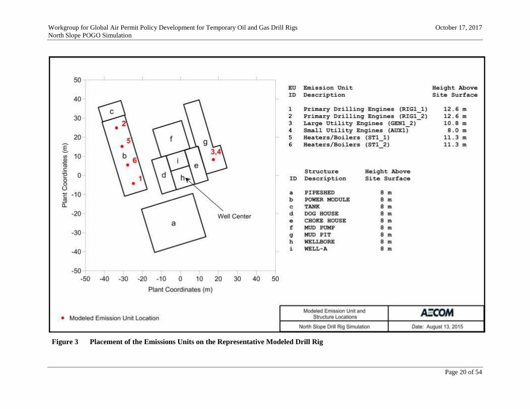
To further describe the modeled EU inventory, the locations of the EUs relative to drill rig
modules, or structures, are illustrated in Figure 3. Figure 4 depicts the proximity of modeled
EUs to drill rig modules and the ambient boundary for each well location modeled. The drill
rig and EUs are arranged for operation along an oil and gas well line. North Slope oil and
gas well lines are often oriented parallel with the prevailing meteorological conditions to
facilitate snow removal.
3.6 Non-Modeled EUs
Table 4 presents examples of EUs that are not explicitly modeled but could occupy the pad
and operate at the same time as the POGO. Some may indirectly support the drilling
operation, and others are equipment permanently located at the pad, such as freeze
protection pumps and production or line heaters. The EUs in Table 4 represent typical
examples of this type of combustion equipment.
Rather than explicit modeling, the Technical Subgroup represented most of the EUs in Table
4 with representative ambient background data. The selection of monitored ambient data to
develop representative background concentrations is discussed in Section 3.13. In addition,
the Technical Subgroup also determined that it was not necessary to model permanent
production heaters or flares as part of the North Slope POGO Simulation but rather address
their influence through a sensitivity modeling analysis. Because of their placement on the
pad relative to the POGO and their stack exit characteristics, these types of equipment are
unlikely to produce plumes of emissions that overlap with the dominate sources of
emissions when a POGO is operating on a well pad. This conclusion was borne out by the
sensitivity modeling analysis conducted; therefore, it was concluded that impacts from a
natural gas-fired production heater and a portable flare do not change the results of the
North Slope POGO Simulation, and these EUs are included as non-modeled sources in
Table 4. This sensitivity analysis for a permanent production heater and portable flare is
discussed in detail in Appendix A.

Workgroup for Global Air Permit Policy Development for Temporary Oil and Gas Drill Rigs October 17, 2017
North Slope POGO Simulation
Page 19 of 54
Table 3 Modeled EU Inventory
Modeled
Stack ID Description Typical Size/Rating
RIG1_1 Primary Drilling Engines
Large (greater than 600 bhp) diesel-fired RICE used for
power generation for rig top drive, rotary table and
draw works, or other electrified equipment.
RIG1_2 Primary Drilling Engines
GEN1_2 Large Utility Engines
Large (greater than 600 bhp) diesel-fired RICE used for
miscellaneous power generation or in mechanical
service driving equipment such as mud pumps, cement
pumps, or grind and inject units.
AUX1 Small Utility Engines Small (less than 600 bhp) diesel-fired RICE used for
miscellaneous power generation or mechanical power.
ST1_1 Drill Rig Heaters and Boilers
Diesel-fired boilers and air heaters used to provide
general utility heat to the drill rig.
ST1_2 Drill Rig Heaters and Boilers
Workgroup for Global Air Permit Policy Development for Temporary Oil and Gas Drill Rigs October 17, 2017
North Slope POGO Simulation
Page 20 of 54
Figure 3 Placement of the Emissions Units on the Representative Modeled Drill Rig

Workgroup for Global Air Permit Policy Development for Temporary Oil and Gas Drill Rigs October 17, 2017
North Slope POGO Simulation
Page 21 of 54
Figure 4 Configuration of the Representative Well Pad with Five Modeled Well (Drill Rig) Locations

Workgroup for Global Air Permit Policy Development for Temporary Oil and Gas Drill Rigs October 17, 2017
North Slope POGO Simulation
Page 22 of 54
Table 4 Example Non-Modeled EUs
Description Description
Oilfield Construction Equipment
Worker housing/camp generators Cranes
Passenger bus Manlifts
Portable heaters Snowblowers
Portable welders Loaders
Portable light plant generators Portable air compressors
Sewage Pump Trucks Portable drills
Tractors Other Mobile Sources
Other portable power generation
Well Drilling, Servicing, Maintenance, and Miscellaneous Oilfield Support Equipment
Worker housing/camp generators Drill rig move engines
Portable light plant generators Graders
Welding, cutting, and soldering equipment Other portable power generation
Coil tubing units N2 pumping units
E-Line/Wireline units Cementing units
Slickline units Hydraulic fracturing units
Hydraulic lifts Hot oil units
Portable Welders Ball mills, grinding mills, and crushers
Bulldozers Portable flares and waste gas incinerators
Cranes Portable incinerators
Manlifts Portable Heaters
Snow blowers, snow melters, and other general
snow removal equipment Other Mobile Sources
Permanent Well Pad Equipment
Production/line heater Small stationary engines in power generation or
mechanical service Freeze protection pumps

Workgroup for Global Air Permit Policy Development for Temporary Oil and Gas Drill Rigs October 17, 2017
North Slope POGO Simulation
Page 23 of 54
3.7 EU Release Parameters
The characterization of emission rates and their release into the atmosphere can significantly
influence model-predicted impacts. Therefore, the following sections provide discussion of
the stack height, diameter, location, and base elevation, in addition to the pollutant emission
rates, exhaust plume exit velocity, and exhaust temperature for each exhaust stack.
3.7.1 Emission Rates
Short-term and long-term emission rates were determined for all modeled EUs for the
North Slope POGO Simulation for a base drill rig fuel consumption of 10,000 gallons
per day. For the purposes of implementing the modeling approach described in
Section 1, all emission rates for any modeled fuel consumption are scaled from these
base emission rates, which are summarized in Table 5. Engine emission rates were
derived from vendor data for non-tiered engines representative of large primary
engines, large utility engines, and small utility engines supporting POGOs. Drill rig
heater and boiler emission rates were calculated based on AP-42 emission factors.13
In
addition to these considerations, emissions, which warrant additional discussion, were
derived based on the information in the following sections.
3.7.1.1 Sulfur Compound Emissions
SO2 emissions are directly related to the sulfur content of the fuel. Since 2006,
all nonroad engines are required to burn ULSD with a maximum sulfur
concentration of 15 parts per million or 0.0015 percent sulfur by weight. While
ULSD is typical for most liquid-fired equipment supporting POGOs on the North
Slope, heaters and boilers are allowed to burn a higher sulfur, Arctic grade fuel,
known as LEPD. To accommodate this range of possible fuels, the North Slope
POGO Simulation drill rig heaters and boilers were assumed to combust LEPD
with a sulfur content of 0.15 percent sulfur by weight.
3.7.1.2 Operational Limits
There are no operational limits assumed in modeling the North Slope POGO
Simulation outside those developed to demonstrate compliance. The Technical
Subgroup assumed all of the modeled EUs are continuously and concurrently
operating during the drilling operation. However, it should be noted that the
purpose of this modeling analysis is to determine operational limits as discussed
with the results in Section 5.
3.7.1.3 Short-Term Emission Rates
The modeled emission rate should generally reflect the maximum emissions
allowed during a given averaging period. Modeled short-term emission rates for
the North Slope POGO Simulation were developed to reflect maximum
emissions by pollutant and averaging period. Short-term emission rates for
1-hour NO2, 1-hour SO2, and 1-hour CO were calculated by multiplying the
13
AP-42, Chapter 1.3 Fuel Oil Combustion; May 2010.

Workgroup for Global Air Permit Policy Development for Temporary Oil and Gas Drill Rigs October 17, 2017
North Slope POGO Simulation
Page 24 of 54
average daily emission rates by a factor of 1.15 to account for short-term
excursions from the daily average emission rate.
3.7.1.4 Application of Temporally-Varying Emissions
Temporally-varying emissions were applied to drill rig operation in two ways to
simulate the following:
Seasonally-varying drill rig equipment operation.
Transient hourly excursions in fuel consumption above the daily modeled
rate.
The use of heaters and boilers supporting a drill rig operation varies seasonally
with higher usage during colder winter months and lower usage during warmer
months. The North Slope POGO Simulation used a seasonal profile of drill rig
heater and boiler usage to simulate this aspect of their operation. To vary the
heater and boiler operation, a monthly nominal emissions scaling factor was
applied to emission rates to simulate the seasonally-varying operation. These
monthly scaling factors are summarized in Table 6.14
In order to maintain a constant drill rig fuel consumption year-round, a
complementary monthly factor was applied to drill rig engine operations, which
is also shown in Table 6. This seasonally-varying operation is conservatively
representative for drill rig engines, because it represents additional fuel
consumption above expected drilling operation during warmer months of the
year. The scaling factors in Table 6 were incorporated into the North Slope
POGO Simulation for all pollutants and averaging periods.
Transient hourly excursions in fuel consumption above the nominal rate were
incorporated into the North Slope POGO Simulation to demonstrate that
conclusions are not sensitive to intermittent operation well above nominal daily
fuel consumption. These excursions were applied by simulating drill rig
operations with 25 percent higher fuel consumption during 20 percent of the
modeled period. The duration of the excursions was randomly chosen according
to a normal distribution with a mean of 48 hours (two days) and standard
deviation of 24 hours (1 day). The length of time at normal operations, without
excursions, was randomly chosen between 0 and 384 hours (16 days). In addition
to emission rates, the modeled exit temperature and exit velocity were also
scaled with the transient hourly excursions by a factor of 1.25 to account for
stack conditions when equipment is running harder. The sensitivity of the North
Slope POGO Simulation to the scaling of these parameters is discussed in
Appendix A. Table 8 summarizes the stack parameters during excursions from
14
The drill rig heater and boiler operational profile follows an approach previously approved by ADEC through
an amendment application submitted for BPXA’s Transportable Drill Rigs Title V Operating Permit
AQ0455TVP01. This information is documented in Figure A-1 of May 11, 2004 letter from Tom Damiana
(SECOR International) to Alan Schuler (ADEC), Re: Response to ADEC Comments Regarding the BP
Exploration (Alaska) Inc. Multiple-Rig Drilling Operations Permit Amendment Application.

Workgroup for Global Air Permit Policy Development for Temporary Oil and Gas Drill Rigs October 17, 2017
North Slope POGO Simulation
Page 25 of 54
nominal operation. The transient hourly excursions were applied to the 1-hour
NO2 modeling only because it was determined to be the limiting pollutant and
averaging period for the North Slope POGO Simulation.
Figure 5 illustrates the emission rate scalars applied within AERMOD over a
typical year to the modeled drill rig engines, heaters, and boilers. The depicted
emission rate scalars include the seasonally-varying operations and transient
hourly excursions applied to the modeling demonstration for 1-hour NO2.
However, the depicted scalars in Figure 5 do not include the constant scalar to
adjust to a fuel consumption basis other than 10,000 gallons per day.
For 1-hour NO2, emission rates for all EUs were applied in AERMOD using an
hourly emissions input file with the “HOUREMIS” keyword to incorporate the
following emission rate refinements: (1) constant scaling to simulate nominal
fuel consumption other than 10,000 gallons per day, (2) seasonal equipment
operations, and (3) transient hourly excursions in emission rates.
For all other pollutants and averaging periods, emission rates for all EUs were
applied in AERMOD using variable emission rate factors with the “EMISFACT”
keyword to incorporate the following emission rate refinements: (1) constant
scaling to simulate nominal fuel consumption other than 10,000 gallons per day
and (2) seasonal equipment operations.
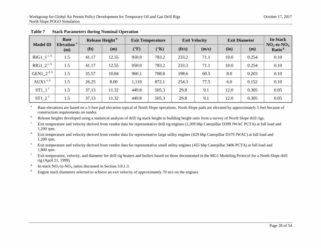
3.7.2 Point Source Parameters
Stack height, stack diameter, location, orientation angle, base elevation, exhaust plume
exit velocity, and exhaust temperature were determined for all modeled EUs. All EUs
are modeled with vertical, uncapped stacks for the North Slope POGO Simulation.
Stack parameters for the North Slope POGO Simulation are summarized in Table 7.
The plant coordinates of EUs modeled at each well location are summarized in Table 9.
The Technical Subgroup collocated stacks for the large and small utility engines,
GEN1_2 and AUX1, respectively. Collocating stacks increases plume overlap and
leads to more conservative modeled impacts.

Workgroup for Global Air Permit Policy Development for Temporary Oil and Gas Drill Rigs October 17, 2017
North Slope POGO Simulation
Page 26 of 54
Table 5 Base Emission Rates (Grams per Second) for a Drill Rig Operating at 10,000 Gallons per Day
Model ID
NO2 SO2 PM2.5 PM10 CO
1-hour Annual 1-hour
3-hour
24-hour
Annual
24-hour Annual 24-hour 1-hour 8-hour
RIG1_1 6.036 5.2491 0.0036 0.0032 0.0418 0.0418 0.0418 0.9863 0.8577
RIG1_2 6.036 5.2491 0.0036 0.0032 0.0418 0.0418 0.0418 0.9863 0.8577
GEN1_2 1.635 1.4215 0.0011 0.0005 0.0206 0.0206 0.0206 0.4893 0.4255
AUX1 0.150 0.1301 0.0001 0.0001 0.0009 0.0009 0.0009 0.0310 0.0269
ST1_1 0.183 0.1587 0.1862 0.1619 0.0169 0.0169 0.0189 0.0456 0.0397
ST1_2 0.183 0.1587 0.1862 0.1619 0.0169 0.0169 0.0189 0.0456 0.0397
Table 6 Nominal Emissions Scaling Factor Used as Input to AERMOD
Month Jan Feb Mar Apr May Jun Jul Aug Sep Oct Nov Dec
Heater/ Boiler
Factor 1.00 1.00 1.00 0.760 0.520 0.280 0.280 0.280 0.460 0.640 0.820 1.00
Engine Factor 1.00 1.00 1.00 1.104 1.208 1.312 1.312 1.312 1.234 1.156 1.078 1.00

Workgroup for Global Air Permit Policy Development for Temporary Oil and Gas Drill Rigs October 17, 2017
North Slope POGO Simulation
Page 27 of 54
Figure 5 Normalized 1-hour NO2 Seasonally-Varying Emission Rates with Transient Hourly
Excursions for (a) Heaters and Boilers and (b) Engines for a Typical Year
0.0
0.2
0.4
0.6
0.8
1.0
1.2
1.4
1.6
1.8
1/1…
3/2…
6/2…
9/1…
12/…
3/1…
6/6…
9/1…
11/…
2/2…
5/2…
8/1…
11/…
2/5…
5/3…
7/2…
10/…
1/1…
4/1…
7/1…
10/…
1/1…
3/2…
6/2…
9/1…
12/…
3/1…
6/7…
9/2…
11/…
2/2…
5/2…
8/1…
11/…
2/6…
5/3…
7/2…
10/…
1/1…
4/1…
7/1…
10/…
1/2…
3/3…
6/2…
9/2…
12/…
3/1…
6/8…
9/3…
11/…
2/2…
5/2…
8/1…
11/…
2/6…
5/4…
7/3…
10/…
1/2…
4/1…
7/1…
10/…
1/3…
3/3…
6/2…
9/2…
12/…
3/1…
6/8…
9/3…
11/…
2/2…
5/2…
8/1…
11/…
2/7…
5/5…
7/3…
10/…
1/2…
4/1…
7/1…
10/…
1/4…
3/3…
6/2…
9/2…
12/…
3/1…
6/9…
9/4…
11/…
2/2…
5/2…
8/1…
11/…
2/8…
5/6…
8/1…
10/…
0.0
0.2
0.4
0.6
0.8
1.0
1.2
1.4
1.6
1.8
Jan Feb Mar Apr May Jun Jul Aug Sep Oct Nov Dec (b)
No
rmal
ize
d S
ho
rt-t
erm
He
ate
r/B
oile
r Em
issi
on
Rat
e
No
rmal
ize
d S
ho
rt-t
erm
En
gin
e E
mis
sio
n R
ate
Jan Feb Mar Apr May Jun Jul Aug Sep Oct Nov Dec (a)
Workgroup for Global Air Permit Policy Development for Temporary Oil and Gas Drill Rigs October 17, 2017
North Slope POGO Simulation
Page 28 of 54
Table 7 Stack Parameters during Nominal Operation
Model ID
Base
Elevation a
(m)
Release Height b Exit Temperature Exit Velocity Exit Diameter In-Stack
NO2-to-NOX
Ratio g (ft) (m) (°F) (°K) (ft/s) (m/s) (in) (m)
RIG1_1 c, h
1.5 41.17 12.55 950.0 783.2 233.2 71.1 10.0 0.254 0.10
RIG1_2 c, h
1.5 41.17 12.55 950.0 783.2 233.3 71.1 10.0 0.254 0.10
GEN1_2 d, h
1.5 35.57 10.84 960.1 788.8 198.6 60.5 8.0 0.203 0.10
AUX1 e, h
1.5 26.25 8.00 1,110 872.1 254.3 77.5 6.0 0.152 0.10
ST1_1 f 1.5 37.13 11.32 449.8 505.3 29.8 9.1 12.0 0.305 0.05
ST1_2 f 1.5 37.13 11.32 449.8 505.3 29.8 9.1 12.0 0.305 0.05
a Base elevations are based on a 5-foot pad elevation typical of North Slope operations. North Slope pads are elevated by approximately 5 feet because of
construction requirements on tundra. b Release heights developed using a statistical analysis of drill rig stack height to building height ratio from a survey of North Slope drill rigs.
c Exit temperature and velocity derived from vendor data for representative drill rig engines (1,309 bhp Caterpillar D399 JWAC PCTA) at full load and
1,200 rpm. d Exit temperature and velocity derived from vendor data for representative large utility engines (629 bhp Caterpillar D379 JWAC) at full load and
1,200 rpm. e Exit temperature and velocity derived from vendor data for representative small utility engines (455 bhp Caterpillar 3406 PCTA) at full load and
1,800 rpm. f Exit temperature, velocity, and diameter for drill rig heaters and boilers based on those documented in the MG1 Modeling Protocol for a North Slope drill
rig (April 21, 1999). g In-stack NO2-to-NOX ratios discussed in Section 3.8.1.3.
h Engine stack diameters selected to achieve an exit velocity of approximately 70 m/s on the engines.

Workgroup for Global Air Permit Policy Development for Temporary Oil and Gas Drill Rigs October 17, 2017
North Slope POGO Simulation
Page 29 of 54
Table 8 Stack Parameters during Excursions from Nominal Operation
Model ID
Base
Elevation a
(m)
Release Height b Exit Temperature Exit Velocity Exit Diameter In-Stack
NO2-to-NOX
Ratio g (ft) (m) (°F) (°K) (ft/s) (m/s) (in) (m)
RIG1_1 c, h
1.5 41.17 12.55 1,303 979.0 291.6 88.9 10.0 0.254 0.10
RIG1_2 c, h
1.5 41.17 12.55 1,303 979.0 291.6 88.9 10.0 0.254 0.10
GEN1_2 d, h
1.5 35.57 10.84 1,315 986.0 248.1 75.6 8.0 0.203 0.10
AUX1 e, h
1.5 26.25 8.00 1,503 1,090 317.8 96.9 6.0 0.152 0.10
ST1_1 f, h
1.5 37.13 11.32 677.3 631.6 37.3 11.4 12.0 0.305 0.05
ST1_2 f, h
1.5 37.13 11.32 677.3 631.6 37.3 11.4 12.0 0.305 0.05
a Base elevations are based on a 5-foot pad elevation typical of North Slope operations. North Slope pads are elevated by approximately 5 feet because of
construction requirements on tundra. b Release heights developed using a statistical analysis of drill rig stack height to building height ratio from a survey of North Slope drill rigs.
c Exit temperature and velocity derived from vendor data for representative drill rig engines (1,309 bhp Caterpillar D399 JWAC PCTA) at full load and
1,200 rpm, scaled by a factor of 1.25 during excursions. d Exit temperature and velocity derived from vendor data for representative large utility engines (629 bhp Caterpillar D379 JWAC) at full load and
1,200 rpm, scaled by a factor of 1.25 during excursions. e Exit temperature and velocity derived from vendor data for representative small utility engines (455 bhp Caterpillar 3406 PCTA) at full load and
1,800 rpm, scaled by a factor of 1.25 during excursions. f Exit temperature, velocity, and diameter for drill rig heaters and boilers based on those documented in the MG1 Modeling Protocol for a North Slope drill
rig (April 21, 1999). Exit temperature and velocity, but not diameter, are scaled by a factor of 1.25 during excursions. It is not appropriate to scale the
diameter as physical changes do not occur to the rig during excursions. g In-stack NO2-to-NOX ratios discussed in Section 3.8.1.3.
h Stack diameters equivalent to those set for Nominal Operation.

Workgroup for Global Air Permit Policy Development for Temporary Oil and Gas Drill Rigs October 17, 2017
North Slope POGO Simulation
Page 30 of 54
Table 9 Location of Emission Releases at Each Drilling Location (Plant Coordinates)
Model ID Well Location 2 (m) Well Location 3 Well Location 4 Well Location 5 Well Location 6
XNorth (m) YEast (m) XNorth (m) YEast (m) XNorth (m) YEast (m) XNorth (m) YEast (m) XNorth (m) YEast (m)
RIG1_1 -140.4 -36.9 -82.6 -20.6 -24.8 -4.2 24.6 9.7 74.0 27.7
RIG1_2 -149.3 -7.8 -91.5 8.6 -33.7 24.9 15.7 38.9 65.1 56.8
GEN1_2 -98.4 -24.5 -40.5 -8.1 17.3 8.3 66.7 22.2 116.0 40.1
AUX1 -98.4 -24.5 -40.5 -8.1 17.3 8.3 66.7 22.2 116.0 40.1
ST1_1 -143.4 -27.2 -85.6 -10.9 -27.7 5.5 21.6 19.5 71.0 37.4
ST1_2 -146.4 -17.5 -88.5 -1.1 -30.7 15.2 18.7 29.2 68.0 47.1

Workgroup for Global Air Permit Policy Development for Temporary Oil and Gas Drill Rigs October 17, 2017
North Slope POGO Simulation
Page 31 of 54
3.8 Pollutant-Specific Considerations
The NO2 and secondarily-formed PM2.5 pollutants warrant additional discussion.
3.8.1 Ambient NO2 Modeling
NOX emissions from combustion sources are partly nitric oxide (NO) and partly NO2.
After the combustion gas exits the stack, additional NO2 can be created due to
atmospheric reactions. Section 5.2.4 of the Guideline (Section 4.2.3.4 of the 2017
Guideline) describes a tiered approach for estimating the annual average NO2 impacts,
ranging from the simplest but very conservative assumption that 100 percent of the NO
is converted to NO2, to other more complex methods.
The Technical Subgroup used the version of the Plume Volume Molar Ratio Method
available as an alternative modeling technique prior to 2017 (pre-2017 PVMRM) to
estimate ambient NO2 concentrations to compare to the 1-hour and annual AAAQS.
Throughout the development of the North Slope POGO Simulation, USEPA had been
adjusting the pre-2017 PVMRM algorithm to better characterize the non-linear mixing
of ozone through the modeled plume. After the modeling was complete, but before
drafting this document, the pre-2017 PVMRM version had been replaced. Because of
the work required in switching the analysis to the current version of PVMRM and pre-
2017 PVMRM was current during the largest part of subgroup efforts, the analysis was
not revised.
3.8.1.1 USEPA and ADEC Approval
The pre-2017 PVMRM approach is a non-Guideline method and required
USEPA and ADEC approval in accordance with 18 AAC 50.215(c)(2). USEPA
Region 10 granted the Workgroup permission to use pre-2017 PVMRM for the
North Slope POGO Simulation on June 28, 2016.15
The Air Permits Program
Manager gave his approval on November 5, 2015.16
3.8.1.2 Public Comment
The use of a non-Guideline model in support of a minor permit decision is
subject to public comment per 40 CFR 51.160(f)(2) and
18 AAC 50.542(d)(1)(F). Therefore, ADEC intends to solicit public comment
regarding the use of pre-2017 PVMRM in the public notice for the preliminary
permit decision.
3.8.1.3 In-Stack NO2-to-NOX Ratio
An in-stack NO2-to-NOX ratio (ISR) must be specified for each modeled EU
when using pre-2017 PVMRM. The Technical Subgroup used an ISR of 0.10 for
15
Letter from David C. Bray (USEPA Region 10) to Alan Schuler (ADEC), dated June 28, 2016.
16 The Commissioner delegated his authority regarding the use of non-guideline models to the Air Permits
Program Manager on June 3, 2008.

Workgroup for Global Air Permit Policy Development for Temporary Oil and Gas Drill Rigs October 17, 2017
North Slope POGO Simulation
Page 32 of 54
all drill rig engines, and an ISR of 0.05 for all drill rig heaters and boilers. The
ISRs are summarized for each modeled EU in Table 7.
The Technical Subgroup used the following data sources to develop the ISRs:
USEPA’s Technology Transfer Network (TTN) Support Center of
Regulatory Atmospheric Modeling (SCRAM) database.17
ADEC’s Air Dispersion Modeling database.18
Measured ISRs compiled in Shell Offshore, Inc.’s (Shell’s) Conical
Drilling Unit Kulluk OCS Permit Applications.19
ISRs for Reciprocating Internal Combustion Engines
For the North Slope POGO Simulation, an ISR of 0.10 was selected for all sizes
of RICE based on the data described in the following studies.
ISR data from USEPA’s SCRAM database for large (greater than 600
horsepower) diesel-fired RICE ranged from 0.06 and 0.10 over various load
classes. ISR data from ADEC’s database are a subset of USEPA’s SCRAM
database and confirmed ISRs less than 0.10 for large RICE. The average ISR
from ADEC’s database was 0.04 across all load classes, with maximum and
minimum ISRs for uncontrolled RICE of 0.05 and 0.03, respectively.
No ISR information exists for small (less than 600 horsepower) diesel-fired
RICE in either the USEPA or ADEC databases. Therefore, ISRs compiled as
supplemental information as part of Shell’s Conical Drilling Unit Kulluk OCS
Permit Applications were examined to determine ISRs for small RICE without
pollution controls. All ISRs for uncontrolled small RICE in Shell’s dataset are
below 0.10, which indicates small RICE have similar ISRs to large RICE.
ISRs for Heaters and Boilers
For the North Slope POGO Simulation, an ISR of 0.05 was selected for all drill
rig heaters and boilers based on the data described in the following studies.
ISR data from USEPA’s SCRAM database for diesel-fired “small” (less than
10 MMBtu/hr heat input) boilers confirm that an ISR as low as 0.05 is justifiable
for the purposes of modeling small diesel fired boilers. An ISR of 0.05 is also
more conservative than the 0.041 ISR used by Shell in their 2011 Conical
Drilling Unit Kulluk OCS Permit Applications.
17
The ISR database on SCRAM may be found at: http://www.epa.gov/ttn/scram/no2_isr_database.htm. 18
ADEC’s ISR database may be found at: http://dec.alaska.gov/air/ap/modeling.htm. 19
Attachment D: Measured NO2/NOx Ratios for Discoverer Source to OCS Permit Applications, Conical Drilling
Unit Kulluk, Beaufort Sea – Supplemental Information, Shell Offshore, Inc. (June 29, 2011).
Workgroup for Global Air Permit Policy Development for Temporary Oil and Gas Drill Rigs October 17, 2017
North Slope POGO Simulation
Page 33 of 54
3.8.1.4 Ozone Data
Pre-2017 PVMRM requires ambient ozone data in order to determine how much
of the NO is converted to NO2. A conservatively representative hourly ozone
dataset was compiled for input into AERMOD from five years of ozone data
collected at BPXA’s A-Pad Monitoring Station between 2006 and 2010. These
years of data were selected for consistency with the meteorological data used for
modeling. This data and the approach to developing this dataset have been
previously approved by ADEC and are routinely used for NO2 modeling of
North Slope sources. One example is the modeling conducted by BPXA in
support of their “Liberty” PSD project (Construction Permit AQ0181CPT06).20
3.8.2 Qualitative Assessment of Secondary PM2.5 Impacts
PM2.5 is either directly emitted from a source or formed secondarily through chemical
reactions in the atmosphere (secondary formation) from other pollutants, such as NOX
and SO2.21
AERMOD is an acceptable model for performing near-field analysis of the
direct emissions, but USEPA has not developed a near-field model that includes the
necessary chemistry algorithms for estimating the secondary impacts. The Technical
Subgroup, therefore, used the USEPA guidance available at the time of the analysis to
address how secondary formation could be accounted for in various PSD scenarios.22
While the guidance is not directed at minor permit modeling, it nevertheless provides
useful information for minor permit assessments.
Following USEPA guidance on addressing secondary PM2.5 formation, secondary
PM2.5 can be qualitatively assessed considering that:
Secondary PM2.5 impacts are not correlated in time or space with direct PM2.5
impacts.
Secondary PM2.5 impacts are captured in the ambient data used for background
concentrations on the North Slope.
Secondary PM2.5 impacts will be small because PM2.5 formation is limited by
low NH3 concentrations on the North Slope.
This USEPA guidance indicates that the maximum direct impacts and the maximum
secondary impacts from a stationary source “…are not likely well-correlated in time or
space.” Therefore, direct and secondary PM2.5 impacts will likely occur in different
locations and at different times because secondary PM2.5 is formed through a complex
photochemical reaction that requires time to occur. This time-frame is too long for
substantial formation to occur in the near-field, which is where the maximum direct
impacts occur. Since the maximum direct project impacts occur within the immediate
20
Additional details regarding the dataset are available in ADEC’s November 22, 2008 modeling review of
BPXA’s ambient demonstration for Liberty.
21 The NOX and SO2 emissions are also referred as “precursor emissions” in a PM2.5 assessment.
22 Guidance for PM2.5 Permit Modeling (EPA-454/B-14-001); May 2014.

Workgroup for Global Air Permit Policy Development for Temporary Oil and Gas Drill Rigs October 17, 2017
North Slope POGO Simulation
Page 34 of 54
near-field of the POGO, the formation of secondary particulates in the near-field of
North Slope POGOs would likely be inconsequential and do not need to be accounted
for in the cumulative impact analysis.
Similarly at larger distances from a source, where the maximum secondary impacts
would occur, direct impacts would be negligible. However, even at these distances, the
maximum secondary PM2.5 impacts expected from a North Slope POGO would also be
very small. This is confirmed by a photochemical modeling study23
that explored the
source-distance relationship of secondary PM2.5 formation from NOX and SO2
precursors. This study showed that maximum secondary PM2.5 impacts from these
precursors occur approximately 5 to 10 kilometers from a source. For a single source
with 1,000 to 3,000 tons per year (tpy) of NOX emissions, 24-hour secondary PM2.5
nitrate impacts would be 0.1 to 1 µg/m3. For a single source with 500 to 1,000 tpy of
SO2 emissions, 24-hour secondary PM2.5 sulfate impacts would be 0.2 to 8 µg/m3. This
study also showed that beyond a distance of 5 to 10 kilometers, secondary PM2.5 sulfate
impacts were negligible. Secondary PM2.5 nitrate impacts were very small, potentially
only as large as 0.2 µg/m3, at a distance of 100 kilometers from the source. Because
direct impacts from a source at these distance would be negligible and the potential
secondary PM2.5 impacts are well below the AAAQS, it is clear that secondary PM2.5
impacts are not a concern.
This study supports conclusions that the magnitude of secondary PM2.5 impacts from
North Slope POGO emissions would be negligible in the immediate near-field of the
POGO where maximum direct PM2.5 impacts occur and small at the location of peak
secondary PM2.5 impacts which are likely to occur beyond five kilometers from the
POGO. Drawing these conclusions for the North Slope POGO from this study is a
conservative application of the study results considering that: (1) North Slope POGO
NOX and SO2 emissions are only a small fraction of source emissions evaluated in this
study and (2) this study was conducted for sources at mid-latitudes which have more
favorable conditions, such as NH3 concentrations, for particulate formation. Formation
of secondary particulates on the North Slope is also limited by low NH3 concentrations.
Therefore, secondary PM2.5 formation in the near-field of the POGO from regional
sources and regionally from the POGO will be small.
USEPA guidance also indicates that representative ambient monitoring data could be
used to address the secondary formation that occurs from existing sources in the
ambient modeling demonstration. The background data used in the PM2.5 AAAQS
analysis in Section 4 adequately meets this objective. As described in Section 3.13, the
ambient data collected is downwind of regional oil and gas operations at a distance that
likely allows for secondary formation of particulates. Therefore, secondary PM2.5
impacts from upwind sources are accounted for in the North Slope POGO Simulation.
23
Baker, K.R., Robert A. Kotchenruther, Rynda C. Hudman. “Estimating ozone and secondary PM2.5 impacts
from hypothetical single source emissions in the central and eastern United States”. Atmospheric Pollution
Research, 2016. 7(1), pp 122-133.

Workgroup for Global Air Permit Policy Development for Temporary Oil and Gas Drill Rigs October 17, 2017
North Slope POGO Simulation
Page 35 of 54
3.9 Downwash
Downwash refers to the situation where local structures influence the plume from an
exhaust stack. Downwash can occur when a stack height is less than a height derived by a
procedure called “Good Engineering Practice” (GEP), which is defined in
18 AAC 50.990(42). It is a consideration when there are receptors relatively near structures
and exhaust stacks.
USEPA developed the “Building Profile Input Program – PRIME” (BPIPPRM) program to
determine which stacks could be influenced by nearby structures and to generate the
cross-sectional profiles needed by AERMOD to determine the resulting downwash. The
North Slope POGO Simulation used the current version of BPIPPRM (version 04274) to
determine the building profiles needed by AERMOD. All modeled point sources are
included in the downwash analysis. BPIPPRM indicated that all modeled exhaust stacks are
within the GEP stack height requirements.
3.10 Ambient Air Boundary
The AAAQS only apply in ambient air locations, which have been defined by USEPA as,
“that portion of the atmosphere, external to buildings, to which the general public has
access.”24
Therefore, areas that are owned or leased by the applicant can be excluded from
the ambient demonstration if public access is “precluded by a fence or other physical
barrier.”25
They conversely need to model that portion of their property/lease that has no
such restriction, or where there is an easement or public right-of-way. Natural features, such
as dense vegetation or topographical features, can provide adequate barriers to public
access, although the adequacy of the given features must be evaluated on a case-specific
basis.
The Technical Subgroup used the edge of the pad as the ambient air boundary, which is
standard practice for North Slope permit applicants. The elevated nature of the gravel pad,
or surrounding berms in the case of ice pads, provides a physical barrier to operations on the
pad. The extent of the well pad and ambient boundary are illustrated in Figure 4 and
Figure 6.
24
The term “ambient air” is defined in 40 CFR 50.1 and adopted by reference in AS 46.14.90(2). 25
USEPA has written a number of guidance documents regarding ambient air issues which may be found in their
Modeling Clearinghouse Information Storage and Retrieval System (MCHISRS) or USEPA Region 7’s “Title
V, NSR/PSD Policy and Guidance Database” (http://cfpub.epa.gov/oarweb/MCHISRS/ and
http://www.epa.gov/region07/air/search.htm). The documents routinely use the phrase “fence or other physical
barrier” when discussing an acceptable means for precluding public access at onshore locations. The phrase
originated in a December 19, 1980 letter from USEPA Administrator Douglas Costle to Senator Jennings
Randolph.

Workgroup for Global Air Permit Policy Development for Temporary Oil and Gas Drill Rigs October 17, 2017
North Slope POGO Simulation
Page 36 of 54
3.11 Receptor Grid
The Technical Subgroup used a rectangular receptor grid of decreasing resolution with
distance from the ambient boundary for modeling with AERMOD. The receptor resolutions
are:
25-meter along the ambient boundary.
25-meter from the ambient boundary to a distance of 100-meter from the ambient
boundary.
50-meter from a distance of 100-meter to 500-meter from the ambient boundary.
Since featureless terrain was simulated at tundra level, as discussed in Section 3.2, all
receptors were modeled with at 0-meter elevation.
Model-predicted impacts were shown to have a steep concentration gradient in the near-field
of the pad, and the maximum impact location was within 100-m of the ambient boundary.
Therefore, this receptor grid is sufficient to define the maximum impacts.
For computational efficiency, the AERMOD receptor grid was further refined for
TRANSVAP post-processing to only consider receptors with the highest
AERMOD-predicted impacts. This process is described along with the development of other
TRANSVAP inputs in Appendix C. Figure 6 illustrates the full AERMOD receptor grid
used in the first steps of the modeling.
3.12 Off-Site Source Impacts and Characterization
The air quality impacts from natural and regional sources, along with long-range transport
from far-field sources, must be accounted for in a cumulative AAAQS demonstration.
Section 8.2 of the Guideline (Section 8.3 of the 2017 Guideline) discusses how the off-site
impacts could be incorporated for purposes of demonstrating compliance with an air quality
standard. Section 8.2.3 (Section 8.3.3 of the 2017 Guideline) recommends that all sources in
the vicinity of the applicant’s source that are not adequately represented by ambient
monitoring data should be explicitly modeled. In general, the Guideline suggests that
sources that cause a significant concentration gradient near the applicant’s source are not
likely to be adequately characterized by the monitored data due to the high degree of spatial
variability of the source’s impact. The impacts from all other sources can be accounted for
through ambient monitoring data. Table 8-1 of the Guideline also allows that, actual
emissions, rather than allowable emissions, may be used to represent the impact from
off-site sources.
The impacts from nearby and far-field off-site sources were accounted for through the
selection of representative background concentrations. Therefore, explicitly modeling these
sources was not required. The selection and representativeness of the monitored ambient
data selected to develop background concentrations is discussed in Section 3.13.

Workgroup for Global Air Permit Policy Development for Temporary Oil and Gas Drill Rigs October 17, 2017
North Slope POGO Simulation
Page 37 of 54
Figure 6 Full AERMOD Receptor Grid

Workgroup for Global Air Permit Policy Development for Temporary Oil and Gas Drill Rigs October 17, 2017
North Slope POGO Simulation
Page 38 of 54
3.13 Ambient Background Concentrations
For a cumulative impact analysis, representative ambient background concentrations must
be developed to combine with model-predicted impacts to account for any non-modeled
emission sources. According to Section 8.2.1 of the Guideline (Section 8.3.1 of the 2017
Guideline), background concentrations should be representative of the following in the
vicinity of the source(s) under consideration:
Natural sources.
Nearby sources other than the one(s) currently under consideration.
Unidentified sources.
For the North Slope POGO Simulation, these sources include those non-modeled mobile,
portable, and intermittent or permanent EUs discussed in Section 3.6 and off-site sources
discussed in Section 3.12. To account for these types of EUs in the North Slope POGO
Simulation, the Technical Subgroup reviewed available North Slope datasets and developed
representative background concentrations using ambient data collected at BPXA’s Well Pad
A (A-Pad) Meteorological and Ambient Air Monitoring Station and at ConocoPhillips
Alaska, Inc.’s (CPAI) Alpine CD1 Ambient Air Quality and Meteorological Monitoring
Station. The A-Pad monitoring station is located on an isolated well pad and therefore, the
ambient data generally represents activities at an isolated well pad (POGO categories RDi
and DDi). The CD1 monitoring station is located on a collocated well pad and therefore, the
data was determined to be representative of activities at a collocated well pad (POGO
categories RDc and DDc) or an isolated well pad with concurrent hydraulic fracturing
activities. The locations of the monitoring stations used to develop the background
concentrations are depicted in Figure 7.
The Technical Subgroup developed separate background concentrations for both isolated
pads and collocated pads for the 1-hour NO2 cumulative impact analysis. For all other
pollutants and averaging periods, the most conservative background concentration available
from either monitor was selected as representative of both isolated and collocated pads. A
summary of ambient background concentrations that are combined with model-predicted
impacts is provided in Table 10 for each modeled pollutant and averaging period.
There are various ways to add a background concentration to the modeled concentration in
an AERMOD analysis. Typical practice is to manually add a single background
concentration to the model-predicted impact as a post-processing step. However, the most
recent versions of AERMOD include options where the background concentration can be
automatically added to the modeled concentration. This option also allows applicants to
include temporarily-varying background concentrations in their ambient demonstrations.
The Technical Subgroup used the manual approach for all pollutants and averaging periods,
except 1-hour NO2, for the North Slope POGO Simulation. The 1-hour NO2 ambient
demonstration used AERMOD’s ability to incorporate temporally-varying background
concentrations that were developed to vary by wind speed, as discussed in Appendix D.

Workgroup for Global Air Permit Policy Development for Temporary Oil and Gas Drill Rigs October 17, 2017
North Slope POGO Simulation
Page 39 of 54
Table 10 Summary of the Background Concentrations Used in the North Slope POGO Simulation
Pollutant Averaging
Period
Monitoring
Station a
Ambient Data Period Applicable POGO
Category Form of the Background Concentration
Background
Concentration d
(ppbv) (µg/m3)
NO2
1-hour
A-Pad 1/1/2008 – 12/31/2012
(5 years) b
RDi, DDi Multi-year average of the 98th
percentile
hourly concentration for each wind speed
category
Varies dependent on
wind speed,
see Appendix D. CD1 10/1/2012 – 9/30/2014
(2 years)
RDc, DDc, and RDi or
DDi with Frac c
Annual CD1 10/1/2012 – 9/30/2014
(2 years) All
Maximum annual average concentration over
the two-year period 9.0 16.9
SO2
1-hour A-Pad
1/1/2010 – 12/31/2012
(3 years) All
Multi-year average of the 99th
percentile of
the annual distribution of daily maximum
concentrations
2.8 7.57
3-hour CD1 10/1/2012 – 9/30/2014
(2 years) All
Maximum 3-hour block average
concentration over the two-year period 8 20.94
24-hour
A-Pad 1/1/2010 – 12/31/2012
(3 years) All
Maximum 24-hour block average
concentration over the three-year period 3.0 7.90
Annual Maximum annual average concentration over
the three-year period 1.0 2.6
PM2.5
24-hour
CD1 10/1/2012 – 9/30/2014
(2 years) All
Multi-year average of the 98th
percentile of
the annual distribution of 24-hour average
concentrations
N/A 15
Annual Maximum annual average concentration over
the two-year period N/A 4.6
PM10 24-hour Maximum 24-hour average concentration
over the two-year period N/A 124
CO
1-hour
CD1 10/1/2012 – 9/30/2014
(2 years) All
Maximum hourly average concentration over
the two-year period 2,000 2,290
8-hour Maximum 8-hour average concentration over
the two-year period 2,000 2,290
a The Technical Subgroup selected the most conservative and available background concentration calculated between the A-Pad and CD1 datasets as representative of isolated
and collocated well pads for all pollutants and averaging periods, except 1-hour NO2. For 1-hour NO2, a unique background concentration was refined for each isolated and
collocated well pads. b All A-Pad ambient air quality data meets PSD-quality data capture requirements, except for hourly NO2 data during the third quarter of 2008, as discussed in Appendix D. c “Frac” means hydraulic fracturing equipment. d Background concentrations from ADEC’s Industrial Data Summary (August 7, 2017) available at: http://dec.alaska.gov/air/ap/modeling.htm.

Workgroup for Global Air Permit Policy Development for Temporary Oil and Gas Drill Rigs October 17, 2017
North Slope POGO Simulation
Page 40 of 54
Figure 7 Meteorological and Ambient Air Monitoring Stations Used for the North Slope POGO Simulation
CD1 MONITORING STATION
APAD MONITORING STATION
BARROW OBSERVATORY

Workgroup for Global Air Permit Policy Development for Temporary Oil and Gas Drill Rigs October 17, 2017
North Slope POGO Simulation
Page 41 of 54
Section 8.2.1.b of the Guideline (Section 8.3.1.b of the 2017 Guideline) indicates that the
ambient data used to develop background concentrations should conform to the
requirements for PSD-quality data. The Technical Subgroup met this requirement with the
A-Pad and CD1 datasets, with one minor exception. One calendar quarter of the five-year
A-Pad NO2 dataset did not meet the 80 percent data capture requirement. The Technical
Subgroup decided to include this quarter of data for the following reasons:
The data capture requirement was already fulfilled through the other four years of
data.
The NO2 data measured in the third quarter of 2008 met all other quality assurance
requirements, except data capture.
Including this additional year of data made the overall dataset more robust.
Sections 3.9 and 3.13.2 further describe relevant aspects of the monitoring sites and the
representativeness of the ambient data selected to develop background concentrations to
support the North Slope POGO Simulation.
3.13.1 A-Pad Ambient Air and Meteorological Monitoring Station
BPXA owns and operates a monitoring station located at A-Pad as part of its PBU
Ambient Air and Meteorological Monitoring Program.26
The A-Pad Monitoring Station
is located approximately 13.5 kilometers northwest of Deadhorse, Alaska, as depicted
in Figure 7. A detailed layout of A-Pad, showing the monitoring station and its location
on the well pad, is included in Appendix D. Because of the location of the monitor and
long history of the monitoring program, BPXA’s A-Pad ambient air quality data is
considered representative of local and regional oil and gas, biogenic, and globally
transported emissions throughout the North Slope and is frequently accepted for use
supporting modeling for North Slope permit applications.
BPXA’s A-Pad is an active well pad with approximately 45 wells that is located at the
edge of the PBU, downwind of several major PBU stationary sources. The location of
the A-Pad Monitoring Station ensures that the station captures regional impacts from
minor stationary, major stationary, and mobile transportation sources associated with
regional oil and gas development. For this reason, A-Pad measurements represent
regional scale impacts from oil and gas development, including impacts from
processing facilities, power stations, drill rigs, well servicing activities, and other
temporary and mobile sources supporting well pad development and maintenance.
The A-Pad Monitoring Station, at its nearest point, is located within 300 feet of the well
line. Therefore, the A-Pad ambient air quality data includes impacts from near-field
emission sources operating at the well pad including drill rigs, well servicing
26
This monitoring program was established in 1986 by BPXA to collect meteorological and ambient air quality
data representative of background concentrations in the PBU. The A-Pad Monitoring Station collects
PSD-quality meteorological data and ambient concentration measurements of oxides of nitrogen (NOX, NO2,
and NO), O3, and SO2 in accordance with its approved Quality Assurance Plan (QAPP). The current QAPP for
the PBU Monitoring Program was approved by ADEC on April 19, 2011.

Workgroup for Global Air Permit Policy Development for Temporary Oil and Gas Drill Rigs October 17, 2017
North Slope POGO Simulation
Page 42 of 54
equipment, camps, mobiles sources, and other portable and temporary equipment, as
summarized in Table 11. The level of activity captured in the measurements is
analogous with current routine infill drilling and well servicing activities on the North
Slope. Although the fuel consumption values listed in Table 11 may appear small
compared to the allowable daily fuel consumption modeled with the North Slope
POGO Simulation, the modeled fuel consumption greatly overstates typical actual
operations.
Based on known activities at A-Pad, the Technical Subgroup determined that the A-Pad
data is directly representative of activities local to an active and isolated well pad
(POGO categories RDi and DDi). However, in many cases, impacts from activities
captured in the A-Pad ambient measurements also result from unidentifiable local
sources of emissions. Figure 8 illustrates the A-Pad hourly NO2 ambient data in relation
to time periods when a drill rig was onsite, the most frequently occurring and highest
measurements occur without a drill rig onsite which clearly indicates that the data is
representative of significant intermittently used oilfield support equipment and
temporary construction activities. While the exact type and length of these activities
varied over time, the Technical Subgroup concluded that the overall level of activity
was adequate for representing most of the non-modeled activities listed in Table 4. The
exception was hydraulic fracturing. Because it is known that limited hydraulic
fracturing occurred at A-Pad during the ambient data period, the Technical Subgroup
decided it was too difficult to justify representing the impacts from this activity with the
A-Pad data and instead represent them using the CD1 ambient data, which is discussed
in Section 3.13.2.
After these considerations, the Technical Subgroup used the A-Pad ambient data to
develop background concentrations for the RDi and DDi POGO categories for the
1-hour NO2 cumulative impact analysis when there are no concurrent hydraulic
fracturing activities. For all other pollutants and averaging periods, the Technical
Subgroup used the A-Pad ambient data as representative of isolated and collocated well
pads (POGO categories RDi, DDi, RDc, and DDc) when it produced a more
conservative background concentration than the CD1 ambient data. This was the case
for 1-hour, 24-hour, and annual SO2.
The Technical Subgroup also determined that because the A-Pad ambient data includes
impacts from periodic drill rig activity, using the A-Pad ambient data to develop
background concentrations double-counts some of the impacts from drill rigs when
included in the North Slope POGO Simulation.
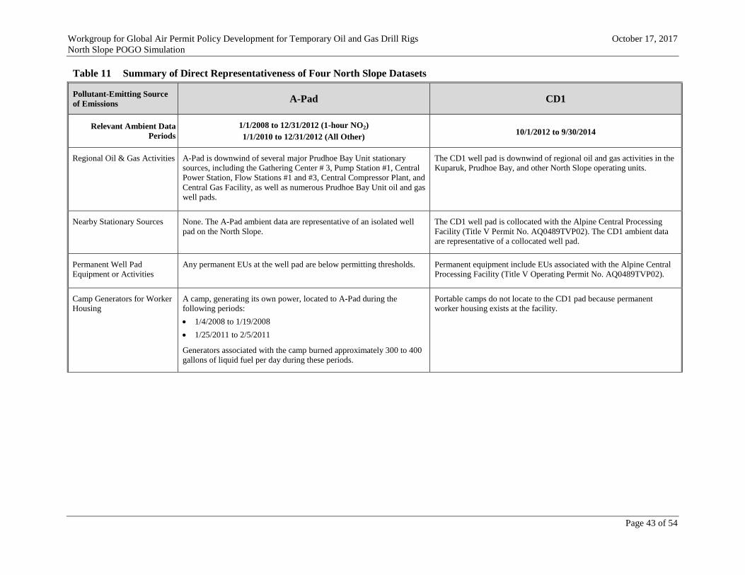
Workgroup for Global Air Permit Policy Development for Temporary Oil and Gas Drill Rigs October 17, 2017
North Slope POGO Simulation
Page 43 of 54
Table 11 Summary of Direct Representativeness of Four North Slope Datasets
Pollutant-Emitting Source
of Emissions A-Pad CD1
Relevant Ambient Data
Periods
1/1/2008 to 12/31/2012 (1-hour NO2)
1/1/2010 to 12/31/2012 (All Other) 10/1/2012 to 9/30/2014
Regional Oil & Gas Activities A-Pad is downwind of several major Prudhoe Bay Unit stationary
sources, including the Gathering Center # 3, Pump Station #1, Central
Power Station, Flow Stations #1 and #3, Central Compressor Plant, and
Central Gas Facility, as well as numerous Prudhoe Bay Unit oil and gas
well pads.
The CD1 well pad is downwind of regional oil and gas activities in the
Kuparuk, Prudhoe Bay, and other North Slope operating units.
Nearby Stationary Sources None. The A-Pad ambient data are representative of an isolated well
pad on the North Slope.
The CD1 well pad is collocated with the Alpine Central Processing
Facility (Title V Permit No. AQ0489TVP02). The CD1 ambient data
are representative of a collocated well pad.
Permanent Well Pad
Equipment or Activities
Any permanent EUs at the well pad are below permitting thresholds. Permanent equipment include EUs associated with the Alpine Central
Processing Facility (Title V Operating Permit No. AQ0489TVP02).
Camp Generators for Worker
Housing
A camp, generating its own power, located to A-Pad during the
following periods:
1/4/2008 to 1/19/2008
1/25/2011 to 2/5/2011
Generators associated with the camp burned approximately 300 to 400
gallons of liquid fuel per day during these periods.
Portable camps do not locate to the CD1 pad because permanent
worker housing exists at the facility.

Workgroup for Global Air Permit Policy Development for Temporary Oil and Gas Drill Rigs October 17, 2017
North Slope POGO Simulation
Page 44 of 54
Table 11 Summary of Direct Representativeness of Four North Slope Datasets
Pollutant-Emitting Source
of Emissions A-Pad CD1
Drill Rig Activities Coiled tubing rigs operated at various wells during the following
periods:
1/4/2008 to 1/21/2008 (Nordic 1)
1/11/2011 to 2/6/2011 (Nordic 2)
These rigs burned anywhere from 1,200 to 2,800 gallons of liquid fuel
per day during these periods.
Other drill rigs operated at various wells on A-Pad during the following
periods:
5/23/2008 to 6/13/2008 (Nabors 4ES)
4/10/2009 to 4/29/2009 (Nabors 7ES)
5/15/2009 to 6/9/2009 (Doyon 16)
7/15/2011 to 8/11/2011 (Doyon 25)
These rigs burned anywhere from 300 to 3,800 gallons of liquid fuel
per day during these periods.
The Doyon19 drill rig operated at various wells during the following
periods:
9/24/2012 to 1/25/2013
5/3/2013 to 7/14/2013
4/24/2014 to 5/29/2014
The drill rig engines operated largely on highline power during these
periods with 1,000 to 4,000 gallons per day of liquid fuel burned by the
drill rig heaters and boilers and other auxiliary or support equipment.
Hydraulic Fracturing and
Well Servicing Activities
The A-26 well was hydraulic fractured on 12/16/2011. Meteorological
conditions indicate that the monitor may not have captured impacts
from the activity.
E-line units, slick-line units, pumping units, coiled tubing units, and/or
other well testing equipment operated sporadically on 473 days
between 2008 and 2012. The location and duration of these activities
varied, depending on the type and level of operation. This equipment
burned liquid fuel.
The CD1-22B, 34, 40, 43, 44, and 47 wells were hydraulically
fractured over 7 days in March 2013 and April 2014. Hydraulic
fracturing activities lasted from 12 to 18 hours per day and consumed
anywhere from 350 and 1,380 gallons of liquid fuel per day.
Meteorological conditions indicate that the monitor captured impacts
from some of these hydraulic fracturing events.
E-line units, slick-line units, hot oil units, and/or coiled tubing units
operated sporadically on 551 days of the ambient data period. The
location and duration of these activities varied, depending on the type
and level of operation. Liquid fuel consumed by equipment associated
with each of these operations ranged from approximately 5 to 300
gallons of fuel per day.
Other Well Pad Equipment
and Activities
Temporary, mobile, and portable equipment. Temporary, mobile, and portable equipment.

Workgroup for Global Air Permit Policy Development for Temporary Oil and Gas Drill Rigs October 17, 2017
North Slope POGO Simulation
Page 45 of 54
Figure 8 Comparison of A-Pad Ambient Data and Drill Rig Activity Onsite
1/1/08 1/1/09 1/1/10 1/1/11 1/1/12

Workgroup for Global Air Permit Policy Development for Temporary Oil and Gas Drill Rigs October 17, 2017
North Slope POGO Simulation
Page 46 of 54
3.13.2 CD1 Ambient Air and Meteorological Monitoring Station
CPAI owns and operates a monitoring station located at its Alpine CD1 Pad.27
The CD1
Pad is located in the Colville River Unit approximately 13 kilometers north of Nuiqsut,
Alaska, as depicted in Figure 7. A detailed layout of the CD1 Monitoring Station and its
location relative to the well pad is included in Appendix D. CPAI’s CD1 ambient air
quality data are considered representative of local and regional oil and gas, biogenic,
and globally transported emissions throughout the North Slope.
The CD1 ambient data includes impacts from the Alpine Central Processing Facility
(CPF), located on the CD1 Pad, which includes operation of natural gas-fired turbines,
natural gas-fired heaters, emergency generators, incinerators, and flares. The facility
has the capability to process three phase liquids (oil, gas, and water) into as much as
139,000 barrels per day of oil for input to the TransAlaska Pipeline system and has an
active airstrip and associated housing for workers. The Alpine CPF is classified as a
PSD-major stationary source for NOx, CO, SO2, PM10, and PM2.5. Actual emissions
from the stationary sources at the Alpine CPF were over 137 tpy CO and 956 tpy NOX
in 2015.
The CD1 Pad also includes an active well line consisting of 48 wells. At its nearest
point, the monitoring station is located within 200 feet of the well line. Therefore, the
CD1 ambient air quality data captures impacts from a variety of equipment involved in
drilling, well development, hydraulic fracturing and well maintenance, including drill
rig engines, drill rig heaters and boilers, well servicing equipment, and other mobile
and portable sources, as summarized in Table 11. The CD1 ambient data does not
directly include impacts from camp generators because most well pads that are
collocated with major stationary sources already include permanent worker housing
facilities. The level of operation described at CD1 is analogous with current drilling and
well servicing activities on the North Slope. Figure 9 presents a visualization of the
timeline of hydraulic fracturing activities at CD1 over the last several years.
Figure 9 Visualization of the Frequency of an Actual Hydraulic Fracturing Operation at the
CD1 Pad
27
Data collection began on October 1, 2012. The CD1 Monitoring Station collects PSD-quality meteorological
data and ambient concentration measurements of CO, NOX, NO2, NO, O3, SO2, PM2.5, and PM10 in accordance
with its approved QAPP. The current QAPP for the CD1 Monitoring Program was approved by ADEC on
September 28, 2012.

Workgroup for Global Air Permit Policy Development for Temporary Oil and Gas Drill Rigs October 17, 2017
North Slope POGO Simulation
Page 47 of 54
Based on the size of the collocated facility, the number of EUs, the presence of an
active well line, and documented portable and mobile source activity, the Technical
Subgroup found the CD1 ambient data to be directly representative of most non-
modeled activities in Table 4 and representative of a collocated well pad. Because of
the increased level of activity and associated impacts, the CD1 ambient data was also
considered representative of isolated well pad POGO categories (RDi and RDc) when
drilling is occurring concurrent with hydraulic fracturing.
After these considerations, the Technical Subgroup used the CD1 ambient data to
develop background concentrations for the RDc and DDc POGO categories and for the
RDi and RDc POGO categories when there is concurrent hydraulic fracturing for the
1-hour NO2 cumulative impact analysis. For all other pollutants and averaging periods,
the Technical Subgroup used the CD1 ambient data as representative of isolated and
collocated well pads (POGO categories RDi, DDi, RDc, and DDc) when it produced a
more conservative background concentration than the A-Pad ambient data. This was the
case for annual NO2, 3-hour SO2, 24-hour PM2.5, annual PM2.5, 24-hour PM10, 1-hour
CO, and 8-hour CO.
The Technical Subgroup also determined that because the CD1 ambient data includes
impacts from periodic drill rig activity, using the CD1 ambient data to develop
background concentrations double-counts some of the impacts from drill rigs when
included in the North Slope POGO Simulation.
3.14 Design Concentrations
USEPA allows the use of modeled concentrations that are consistent with the form of the
standard for design concentrations. The allowed design concentrations when using five
years of meteorological data are summarized in Table 12, along with applicable AAAQS
and NAAQS evaluated for the North Slope POGO Simulation. The Technical Subgroup
evaluated model-predicted impacts against the AAAQS with design concentrations at least
as conservative as the values described in Table 12.
3.15 Post-Processing
AERMOD output for 1-hour NO2 and 1-hour SO2 modeling demonstrations for the North
Slope POGO Simulation was post-processed with TRANSVAP to better simulate the
transitory nature of the portable sources. AERMOD-predicted impacts for all other
pollutants and averaging periods were analyzed for the North Slope POGO Simulation
without further processing. Additional information about the TRANSVAP post-processor
and input development for TRANSVAP is discussed in Appendix C.

Workgroup for Global Air Permit Policy Development for Temporary Oil and Gas Drill Rigs October 17, 2017
North Slope POGO Simulation
Page 48 of 54
Table 12 Allowed Design Concentrations and Applicable AAAQS and NAAQS
Pollutant Averaging
Period
Modeled Design Value to Compare to
AAAQS and NAAAQS AAAQS NAAQS
NO2
1-hour 5-year average of the high-eighth-high daily
maximum 1-hour average concentration 188 µg/m
3
100 ppbv
(188 µg/m3)
Annual Maximum annual average concentration
from any modeled year 100 µg/m
3
53 ppbv
(100 µg/m3)
SO2
1-hour 5-year average of the high-fourth-high daily
maximum 1-hour average concentration 196 µg/m
3
75 ppbv
(196 µg/m3)
3-hour a
Maximum high-second-high 3-hour average
concentration from any year 1,300 µg/m
3
0.5 ppmv
(1,300 µg/m3)
24-hour a
Maximum high-second-high 24-hour
average concentration from any year 365 µg/m
3 N/A
Annual Maximum annual average concentration
from any modeled year 80 µg/m
3 N/A
PM2.5
24-hour 5-year average of the high-eighth-high
24-hour average concentration 35 µg/m
3 35 µg/m
3
Annual 5-year average of the annual average
concentrations 12 µg/m
3 12 µg/m
3
PM10 24-hour a
High-sixth-high 24-hour average
concentration over 5 years 150 µg/m
3 150 µg/m
3
CO
1-hour a
Maximum high-second-high 1-hour average
concentration from any year 40 mg/m
3
35 ppm
(40 mg/m3)
8-hour a
Maximum high-second-high 8-hour average
concentration from any year 10 mg/m
3
9 ppm
(10 mg/m3)
a For the North Slope POGO Simulation, the design concentration for this pollutant and averaging period was
simulated as the highest-second-high concentration over the entire five-year model simulation, which is more
conservative than the allowable design concentration.

Workgroup for Global Air Permit Policy Development for Temporary Oil and Gas Drill Rigs October 17, 2017
North Slope POGO Simulation
Page 49 of 54
4. RESULTS AND DISCUSSION
The maximum modeled-predicted impacts from the North Slope POGO Simulation are presented
in Figure 10 and Table 13. The background concentration, maximum model-predicted impact for
each fuel consumption simulated, and respective ambient standard are also presented for
comparison. The model-predicted impacts are used to find the maximum allowable drill rig
operation that does not cause or contribute to a violation of the AAAQS using the modeling
approach discussed in Section 1.
4.1 Conservatism in the Modeling Demonstration
The North Slope POGO Simulation was developed to be conservatively representative of a
POGO operating on the North Slope. However, the following aspects of the simulation
should also provide reasonable assurance that the AAAQS will not be violated and are
worth noting when interpreting results:
The simulation included a drill rig operating at five potential well locations at a well
pad. Many North Slope well pads have 15 or more wells. Modeling fewer wells than
exist in reality will lead to overstating actual impacts because each well location
represents three or more wells, which increases the probability of drill rig impacts
occurring in the same location. The simulation will also overstate the impacts for
activities involving less than five wells, such as exploratory programs, because more
activity is simulated at a well pad than what would be expected if drilling only a few
wells.
The drill rig is modeled operating on a 320-meter by 105-meter (11.9 acre) well pad,
within 25 meters of the well pad ambient boundary. This is representative of distances
to pad edge on the smallest pads on the North Slope. A small pad means that stacks
are simulated closer to ambient air. Well pads on the North Slope range from as small
as six acres (with fewer than 20 wells) in newer developments to larger than 80 acres
in older developments, such as Prudhoe Bay.
Well Location 6 is located closer to the side of the well pad ambient boundary where
the maximum impacts are predicted, which adds additional conservativism to model-
predicted impacts.
The drill rig heaters and boilers burn LEPD, which has a higher sulfur content than
ULSD. On the North Slope, many POGOs do not have access to LEPD because its
use is restricted by access to a North Slope topping plant. Therefore, predicted SO2
impacts dominated by North Slope POGO heaters and boilers are potentially 100
times higher than what occurs at many North Slope locations. For locations accessible
from a North Slope topping plant, the sulfur content of LEPD is prescribed by permit
restrictions for sulfur content at other stationary sources that receive and burn LEPD.
Based on current conditions, North Slope topping plants are producing LEPD fuels
with a sulfur content of 0.11 percent by weight or less. LEPD for the North Slope
POGO Simulation was characterized with a sulfur content of 0.15 percent by weight.

Workgroup for Global Air Permit Policy Development for Temporary Oil and Gas Drill Rigs October 17, 2017
North Slope POGO Simulation
Page 50 of 54
The drill rig heaters and boilers were modeled with a seasonal operational profile
using monthly scaling factors. In order to maintain a constant drill rig fuel
consumption year-round, a complementary monthly factor was applied to the drill rig
engines. While assuming a seasonal variation in drill rig heater and boiler operation is
less conservative than assuming a constant value, the complementary seasonal
variation in drill rig engine operations is not. It is not expected that drill rig engines
will operate more when heaters and boilers operate less. This will over predict
impacts from drill rig engines during warmer months of the year than would
reasonably be anticipated with less heater and boiler operation.
All EUs are modeled operating concurrently.
TRANSVAP post-processing requires the use of activity input files to simulate a drill
rig operating at different locations and the duration of active drilling and inactivity at
a well pad. For the routine infill drilling activity profile, these activity inputs are
based on actual North Slope drill rig activity data. Additional conservatism is built
into the analysis of this data by including drill rig activities that are not necessarily
representative of routine infill drilling. The dataset developed includes activities
performed by drill rigs supporting developmental drilling events. Including these
activities in the data has the effect of increasing the duration of time a well pad is
active.
Although the 1-hour NO2 and 1-hour SO2 modeling demonstrations incorporated
several refinements, demonstrations for all other pollutants and averaging periods
were conducted with the standard, simplified modeling approach. For modeling a drill
rig, this includes modeling year-round operations (8,760 hours per year) at a single
location and combining model-predicted impacts with a constant background value
determined from ambient data.
Background concentrations developed from A-Pad and CD1 ambient datasets include
impacts from drill rigs, which were also explicitly modeled in the ambient
demonstration for the North Slope POGO Simulation. Therefore, there is some
amount of double-counting drill rig impacts. Based on drill rig fuel use data collected
between 2006 and 2011 during operations at A-Pad, typical drill rig fuel use was
1,760 gallons per day on average and as high as 3,840 gallons per day.
PVMRM requires ambient ozone data in order to determine how much of the NO is
converted to NO2. A conservatively representative hourly ozone dataset was compiled
for input into AERMOD from five years of ozone data collected at BPXA’s A-Pad
Monitoring Station between 2006 and 2010. This increases conversion to NO2.
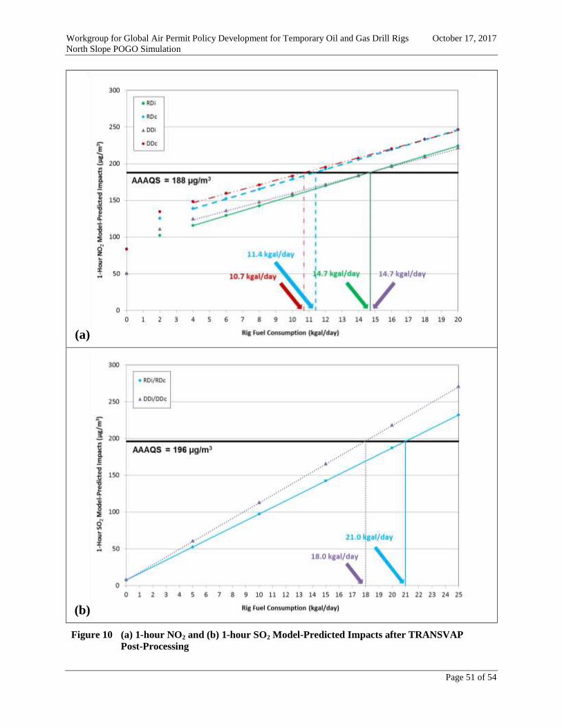
Workgroup for Global Air Permit Policy Development for Temporary Oil and Gas Drill Rigs October 17, 2017
North Slope POGO Simulation
Page 51 of 54
Figure 10 (a) 1-hour NO2 and (b) 1-hour SO2 Model-Predicted Impacts after TRANSVAP
Post-Processing
(a)
(b)

Workgroup for Global Air Permit Policy Development for Temporary Oil and Gas Drill Rigs October 17, 2017
North Slope POGO Simulation
Page 52 of 54
Table 13 Summary of Results
Pollutant Averaging
Period
Model and
Post-Processor
(if applicable)
AERMOD Results (µg/m3)
for Each Fuel Consumption (kgal/day)
Background
Concentration
(µg/m3)
AAAQS/
NAAQS
(µg/m3)
Nominal Fuel Consumption to
Predict Impacts as
High as the AAAQS
(kgal/day)
0 5 10 15 20 25 RDi RDc DDi DDc
NO2
1-hour
AERMOD
(version 15181)
TRANSVAP
See Figure 10(a).
Varies with
wind speed, see
Appendix D.
188 14.7 11.4 14.7 10.7
Annual AERMOD
(version 15181) 0.0 8.5 11.8 15.3 18.7 21.9 16.9 100 116.2
SO2
1-hour
AERMOD
(version 14134)
TRANSVAP
See Figure 10(b). 7.57 196 21.0 18.0
3-hour
AERMOD
(version 14134)
0.0 62.1 124.2 186.3 248.4 310.6 20.94 1,300 103.0
24-hour 0.0 44.6 89.2 133.8 178.5 223.1 7.90 365 40.0
Annual 0.0 3.0 6.0 9.0 12.0 14.9 2.6 80 129.4
PM2.5
24-hour AERMOD
(version 15181) 0.0 2.7 5.5 8.2 10.9 13.6 15 35 36.7
Annual
AERMOD
(version 14134)
0.0 0.4 0.8 1.2 1.6 2.0 4.6 12 90.5
PM10 24-hour 0.0 5.2 10.4 15.6 20.8 26.0 124 150 25.0
CO
1-hour 0.0 129.1 258.2 387.2 516.3 645.4 2,290 40,000 1,461
8-hour 0.0 69.3 138.7 208.0 277.4 346.7 2,290 10,000 555.9
Allowable Nominal Fuel Consumption 14.7 11.4 14.7 10.7

Workgroup for Global Air Permit Policy Development for Temporary Oil and Gas Drill Rigs October 17, 2017
North Slope POGO Simulation
Page 53 of 54
5. CONCLUSIONS
The North Slope POGO Simulation was developed to be representative of any POGO on the
North Slope. The modeling analysis was conducted in a manner consistent with the Guideline, as
required under 18AAC 50.215(b)(1). The following sections summarize the key parameters and
assumptions used in the North Slope POGO Simulation and the results of the modeling analysis.
5.1 Summary of Key Parameters and Assumptions
The following list summarizes key parameters and assumptions used in the North Slope
POGO Simulation. For this analysis, the Technical Subgroup:
Simulated onshore POGOs at well pads on the North Slope coastal plain, where
POGO activities occur on a “small” pad, and the ambient boundary is at pad edge.
Addressed four POGO categories including routine infill drilling at an isolated well
pad (RDi) or a collocated well pad (RDc) and developmental drilling at an isolated
well pad (DDi) or collocated well pad (DDc).
Included nonroad drill rig engines that meet past or present federal emission
requirements (Tier 0 to Tier 4).
Modeled fuel consumption only applies to primary units permanently attached to or
integral to the drill rig, and all other ancillary equipment are adequately represented
through the background data and did not need to be explicitly modeled.
Assumed all modeled and non-modeled POGO EUs are liquid-fired and that all of the
internal combustion units are reciprocating engines.
Assumed the total volume of fuel consumed by the modeled drill rig RICE and
heater/boiler EUs does not exceed the levels shown in Table 14.
Simulated the sulfur content of the liquid fuel as:
o ≤ 0.0015 percent by weight (ULSD) for the fuel consumed by the RICE EUs.
o ≤ 0.15 percent by weight (LEPD) for the fuel consumed by the heaters/boilers.
Assumed rig emissions are linearly-correlated to fuel consumption.
Assumed that the operation of the drill rig heaters and boilers vary seasonally but do
not exceed 30 percent of the levels shown in Table 14.
Characterized the modeled exhaust stacks of the drill rig RICE and heater/boiler EUs
as vertical and uncapped, with stack heights that represent the current existing stack
heights of North Slope drill rigs.

Workgroup for Global Air Permit Policy Development for Temporary Oil and Gas Drill Rigs October 17, 2017
North Slope POGO Simulation
Page 54 of 54
Did not conduct modeling to demonstrate compliance with the maximum allowable
increases listed in 18 AAC 50.020.
Assumed that air quality impacts from equipment outlined in Table 4 are adequately
represented through background ambient data, or the sensitivity analysis provided in
Appendix A, and did not need to be explicitly modeled. These equipment include:
o oilfield construction equipment.
o well drilling, hydraulic fracturing, well servicing, maintenance, and miscellaneous
oilfield support equipment.
o stationary well pad equipment, including a production or line heater, freeze
protection pump, or other small stationary engines used to power generation or
mechanical service to support well pad activities.
Assumed the hydraulic fracturing impacts captured in the background data are only
representative of those from activities used in the development of conventional
resources.
5.2 Summary of Conclusions
Based on the results of the modeling analysis developed for the North Slope POGO
Simulation, the level of drill rig operations described in Table 14 will not cause or
contribute to a violation of the AAAQS listed in Section 1 of this report.
Table 14 Maximum
b Modeled Quantity of Fuel That a North Slope POGO
a Could
Consume Without Violating an AAAQS (Gallons per Day)
Allowable Onshore Drill Rig Operation RDi b RDc
b DDi
b DDc
b
POGO Without Concurrent Hydraulic Fracturing Activities c 14,700 11,400 14,700 10,700
POGO With Concurrent Hydraulic Fracturing Activities c 11,400 11,400 10,700 10,700
a Daily fuel consumption thresholds apply to the drill rig only and do not apply to other emission units
that may be a part of the POGO or operating on the well pad, such as stationary well pad equipment,
portable power generators, or well servicing equipment (as defined in 18 AAC 50.990(125)) – these
activities are represented by the background values added to the modeled impacts. An example list of
this equipment is outlined in Table 4. b Daily fuel consumption thresholds can be exceeded by 25 percent, 20 percent of the days in a year
(73 days per year), which is equivalent to the following daily volumes:
14,700 x 1.25 = 18,375 gallons per day.
11,400 x 1.25 = 14,250 gallons per day.
10,700 x 1.25 = 13,375 gallons per day. c Hydraulic fracturing in Alaska is discussed in Appendix E.

Prepared by: AECOM
October 17, 2017
Appendix A
AERMOD Sensitivity Analyses

Workgroup for Global Air Permit Policy Development for Temporary Oil and Gas Drill Rigs October 17, 2017
North Slope POGO Simulation
Page A1 of A11
A1. SENSITIVITY OF MODEL-PREDICTED IMPACTS TO AERMOD
UPDATES BETWEEN VERSIONS 14134, 15181, AND 16216R
As the Technical Subgroup was finalizing the North Slope POGO Simulation, USEPA
promulgated new versions of AERMET (versions 15181 and 16216) and AERMOD
(version 15181 and 16216r). This analysis describes a limited study conducted to demonstrate
that assessments conducted with the superseded versions of AERMOD and AERMET yield the
same results as those conducted with the current versions (16216r and 16216, respectively),
obviating the need to revise all analyses conducted with the previous versions of AERMOD and
AERMET. To conduct this study, a sensitivity analysis was conducted for 1-hour NOX, 1-hour
SO2, and 24-hour PM2.5 to compare the potential influence of any updates to algorithms between
AERMOD and AERMET versions 14134, 15181, and 16216r (16216). The sensitivity analysis
was conducted for NOX rather than NO2 because the PVMRM chemical algorithms in AERMOD
version 15181, are no longer available with version 16216r. Therefore, a direct comparison is not
possible. Table A1 compares AERMOD-predicted impacts for the North Slope POGO
Simulation. These results indicate there are no discernible differences to the AERMOD-predicted
1-hour NOX, 1-hour SO2, and 24-hour PM2.5 impacts between processing with AERMOD
versions 14134, 15181, and 16216r.
Table A1 Comparison of 1-hour NOX, 1-hour SO2, and 24-hour PM2.5 Impacts Modeled with AERMOD Versions 14134, 15181, and 16216r
Nominal Fuel
Consumption Modeled
(kgal/day)
AERMOD-Predicted Design Values (µg/m3)
Version 14134 Version 15181 Version 16216r
1-hour NOX
5 493.88051 493.88051 493.88051
10 987.76102 987.76102 987.76102
15 1481.64152 1481.64152 1481.64152
20 1975.52203 1975.52203 1975.52203
25 2469.40254 2469.40254 2469.40254
1-hour SO2
5 69.86519 69.86519 69.86519
10 139.73038 139.73038 139.73038
15 209.59556 209.59556 209.59556
20 279.46075 279.46075 279.46075
25 349.32594 349.32594 349.32594
24-hour PM2.5
5 2.72593 2.72593 2.72593
10 5.45187 5.45187 5.45187
15 8.1778 8.1778 8.1778
20 10.90374 10.90374 10.90374
25 13.62967 13.62967 13.62967
Workgroup for Global Air Permit Policy Development for Temporary Oil and Gas Drill Rigs October 17, 2017
North Slope POGO Simulation
Page A2 of A11
A2. SENSITIVITY OF MODEL-PREDICTED IMPACTS TO
NON-TIERED VERSUS TIER 4 DRILL RIG ENGINES
The North Slope POGO Simulation was developed with drill rig equipment and emissions
representative of current drill rigs operating on the North Slope. However, future POGOs will
include equipment subject to continually more stringent emission standards and equipment
regulations leading to lower polluting operations. However, for nonroad engines, designing
cleaner burning equipment with respect to NOX and PM emissions can lead to an increase in the
portion of NOX that is NO2. For future operations, this warrants further investigation because the
National Ambient Air Quality Standard (NAAQS) regulates NO2. Therefore, in an effort to
confirm the North Slope POGO Simulation modeling results are applicable for future operations,
a 1-hour NO2 analysis was conducted comparing impacts from drill rig engines representative of
current operations to impacts from Tier 4 drill rig engines. This type of analysis was not carried
out for the other major class of equipment in the North Slope POGO Simulation, heaters and
boilers, because there are not similar concerns.
A2.1 Background
Representative drill rig emissions were developed for the North Slope POGO Simulation
with non-tiered engines from Caterpillar vendor data. For this demonstration, impacts from
the non-tiered, vendor-supplied drill rig engine emissions are compared to impacts from
Tier 4 drill rig engine emissions, which must comply with a more stringent NOX emission
standard.28
While the NOX emissions from these engines are lower, they are expected to
have higher in-stack NO2-to-NOX ratios (ISRs) than non-tiered engines because of catalyzed
diesel particulate filters.
Tier 4 engine emissions were derived using the emission standards in 40 CFR 1039.101 and
adding an additional 25 percent, or factor of 1.25, to represent not-to-exceed (NTE)
emission rates consistent with the NTE basis for the vendor-supplied non-tiered engines.
The primary drill rig engines are assumed to be in generator service while the large and
small utility engines are assumed to be in mechanical service. For Tier 4 engines, an ISR of
0.30 is conservatively assumed for this demonstration. For modeling purposes, the only
model parameters that change are estimated emissions and ISR between simulations with
the non-tiered and Tier 4 engines. Table A2 compares estimated emissions and ISRs for the
non-tiered and Tier 4 drill rig engines. The NOX emission rates in Table A2 are calculated
based on a nominal fuel consumption of 10,000 gallons per day.
28
Tier 4 emissions standards in 40 CFR 1039.101, Table 1, Tier 4 Exhaust Emission Standards After the 2014
Model Year, g/kW-hr.

Workgroup for Global Air Permit Policy Development for Temporary Oil and Gas Drill Rigs October 17, 2017
North Slope POGO Simulation
Page A3 of A11
Table A2 Comparison of Non-Tiered and Tier 4 Engine Emission Rates and Model
Parameters for Sensitivity Analysis
Source
ID Source Description
North Slope Non-Tiered
Drill Rig Engines Tier 4 Drill Rig Engines
NOX Emission
Rate
(g NOX/s)
In-Stack
NO2-to-NOx
Ratio
NOX Emission
Rate
(g NOX/s)
In-Stack
NO2-to-NOx
Ratio
RIG1_1 Primary Drilling Engines 6.036 0.07 0.466 0.30
RIG1_2 Primary Drilling Engines 6.036 0.07 0.466 0.30
GEN1_2 Large Utility Engines 1.635 0.07 0.727 0.30
AUX1 Small Utility Engines 0.150 0.07 0.011 0.30
This modeling demonstration is conducted using the PVMRM option with AERMOD and
all other model parameters developed for the North Slope POGO Simulation as discussed in
the modeling report. For simplicity in this demonstration, impacts are compared using
AERMOD results only; results were not post-processed with TRANSVAP. In addition, to
evaluate the differences specific to the drill rig engines:
All other non-engine sources, such as boilers and heaters, have zero emissions.
No ambient background concentrations were incorporated into the AERMOD results.
By removing the emissions from all other sources, except for the engines, this analysis is
focused on the engines.
A2.2 Results
Table A3 compares the modeled impacts from the non-tiered and Tier 4 drill rig engines
given the assumptions outlined in Section A3.1 for the five well (drill rig) locations modeled
for the North Slope POGO Simulation. The ratio of Tier 4 to non-tiered engine impacts in
Table A3 is calculated as follows:
Ratio of Tier 4 to Non-Tiered Engine Impacts = Tier 4 Engine Impacts at Max Receptor
Non-Tiered Engine Impacts at Max Receptor
Note that the modeled receptor with the maximum impact may be different between
simulations. In all cases in Table A3, impacts from Tier 4 drill rig engines are only a
fraction of impacts from the non-tiered drill rig engines. The ratio of Tier 4 to non-tiered
engine impacts varies with emissions based nominal daily fuel consumption. Therefore,
impacts were predicted using several daily fuels consumption values spanning the range of
those potentially proposed as limits. At the extreme upper limit of potential daily fuel
consumption modeled, the Tier 4 engine model-predicted impacts are most similar to
non-tiered impacts. Yet, the high-eighth-high (H8H) Tier 4 engine impacts are less than

Workgroup for Global Air Permit Policy Development for Temporary Oil and Gas Drill Rigs October 17, 2017
North Slope POGO Simulation
Page A4 of A11
76 percent of non-tiered engine impacts across all modeled drill rig locations. Therefore, for
any reasonably expected amount of drill rig operation, the modeling developed with non-
tiered engine emissions conservatively represents potential future operations with Tier 4 or
better drill rig engines. This demonstration shows the North Slope POGO Simulation is
applicable to future operations.
Table A3 Ratio of Tier 4 to Non-Tiered Drill Rig Engine 1-Hour NO2 Impacts
Modeled
Well Pad
Location
Ratio of Tier 4 to Non-Tiered Engine Impacts
5 kgal/day
Nominal Fuel Consumption
15 kgal/day
Nominal Fuel Consumption
25 kgal/day
Nominal Fuel Consumption
H1H 1 H8H
2 H1H
1 H8H
2 H1H
1 H8H
2
2 0.53 0.49 0.70 0.73 0.66 0.76
3 0.48 0.45 0.79 0.71 0.90 0.73
4 0.45 0.46 0.76 0.72 0.91 0.74
5 0.45 0.47 0.76 0.72 0.91 0.74
6 0.45 0.43 0.76 0.66 0.89 0.68
1 High-First-High (H1H) 1-hour NO2 results are based on the ratio of first-highest maximum daily 1-hour NO2
results averaged over five years.
2 High-Eighth-High (H8H) 1-hour NO2 results are based on the ratio of eighth-highest maximum daily 1-hour
NO2 results averaged over five years (design value).
A3. SENSTIVITY OF MODEL-PREDICTED IMPACTS TO STACK
PARAMETERS DURING EXCURSIONS
For the cumulative impact analysis for the North Slope POGO Simulation, temporally-varying
emissions were applied to drill rig operation to simulate transient hourly excursions in fuel
consumption above the nominal modeled daily rate. In the North Slope POGO Simulation
modeling report, these are referred to as “excursions.” For modeling purposes, an excursion is
equivalent to a 25 percent increase in drill rig fuel consumption (emissions), which occurs
sporadically 20 percent of the time during the five-year simulation. Concurrent with the
excursions in drill rig fuel consumption, a 25 percent increase in the exit temperature and exit
velocity stack parameters was also applied in the modeling. This memorandum addresses
concerns that these stack parameter assumptions may understate model-predicted impacts and
discusses the sensitivity of the modeling demonstration to those assumptions.
A3.1 Stack Parameters for Modeling
For the North Slope POGO Simulation, two stack parameters, exit temperature and exit
velocity, were scaled by a factor of 1.25, concurrent with the scaling of modeled emission
rates for excursions. Table A4 compares the difference in exit temperature and exit velocity
between periods of nominal operations and periods of excursions from nominal operations.
All other stack parameters, including release height, exit diameter, and in-stack NO2-to-NOX
ratio, remain the same under both operational conditions.

Workgroup for Global Air Permit Policy Development for Temporary Oil and Gas Drill Rigs October 17, 2017
North Slope POGO Simulation
Page A5 of A11
Table A4 Comparison of Stack Parameters during Nominal Operations and Excursions from
Nominal Operations
Model
ID
Exit Temperature Exit Velocity
Nominal
Operations
(No Scaling)
Excursions
(1.25 Factor)
Nominal
Operations
(No Scaling)
Excursions
(1.25 Factor)
(°F) (°K) (°F) (°K) (ft/s) (m/s) (ft/s) (m/s)
RIG1_1 950.0 783.2 1,303 979.0 233.2 71.1 291.6 88.9
RIG1_2 950.0 783.2 1,303 979.0 233.2 71.1 291.6 88.9
GEN1_2 960.2 788.8 1,315 986.0 198.6 60.5 248.1 75.6
AUX1 1,110 872.1 1,503 1,090 254.3 77.5 317.8 96.9
ST1_1 449.8 505.3 677.3 631.6 29.8 9.1 37.3 11.4
ST1_2 449.8 505.3 677.3 631.6 29.8 9.1 37.3 11.4
A3.2 Results and Discussion
A sensitivity analysis was conducted to explore how the model-predicted impacts are
influenced by the difference in exit temperature and exit velocity between nominal
operations and excursions from nominal operations. The sensitivity analysis was conducted
with the 1-hour NO2 modeling demonstration because it is the limiting pollutant and
averaging period identified for the North Slope POGO Simulation, and consequently, it is
also the only ambient demonstration that included excursions. Table A5 summarizes
cumulative model-predicted impacts for the North Slope POGO Simulation, modeled with
two different stack parameter scenarios during excursions: (1) scaling both exit temperature
and exit velocity and (2) scaling exit velocity only. These stack parameter scenarios are only
applicable to the 20 percent of the time that is simulated as excursions. No scaling is applied
to stack parameters during the other 80 percent of the time which was modeled as nominal
operations.
ADEC has noted that simulating an increase in flow rate (exit velocity) during excursions is
a reasonable assumption for reciprocating internal combustion engines (RICE) and external
combustion units. ADEC also noted that while temperature may also increase with load, the
magnitude or character of that increase is unclear. However, the results in Table A5 show
that the cumulative impact analysis for the North Slope POGO Simulation is not sensitive to
the scaling of exit temperature. Whether exit temperature and exit velocity or exit velocity
only is scaled during excursions, there is little difference in the model-predicted impacts.

Workgroup for Global Air Permit Policy Development for Temporary Oil and Gas Drill Rigs October 17, 2017
North Slope POGO Simulation
Page A6 of A11
Table A5 Comparison of Model-Predicted Impacts for the RDi POGO Category
Description of Processing Form of the Model
Predicted Impact
Cumulative Model-Predicted Impact a
(µg/m3)
Exit Temperature and
Exit Velocity Scaled Exit Velocity
AERMODb Only
Highest-eighth-high
from all rig locations 214.00 211.35
AERMODb + TRANSVAP
Post-Processing 99
th Percentile 169.87 170.01
a Cumulative model-predicted impacts are based 12,000 gallons per day of drill rig operation and includes the
background concentration for the RDi POGO Category.
b Version 15181 was used for consistency with the North Slope POGO Simulation.
Also of note are the AERMOD-predicted impacts with exit temperature and exit velocity
scaled compared to the impacts with exit velocity only scaled. Cumulative
AERMOD-predicted impacts appear to improve when scaling of the exit temperature during
excursions is removed from the analysis. Because higher exit temperatures are expected to
improve dispersion characteristics of the plume due to buoyancy, there may be other
explanations for the results:
(1) Changing the exit temperature may alter the dispersion of the plume to the extent
that it shifts maximum impacts in relation to the receptors, or
(2) Changing the exit temperature may alter, temporally, which days contribute to the
daily maximum 1-hour NO2 concentrations in the annual distribution of daily
maximums for each year of the simulation. This is worth noting considering that
background concentrations are dependent on wind speed, and therefore, also vary
temporally.
A3.3 Stack Parameters for Modeling
The sensitivity analysis indicates that the North Slope POGO Simulation model-predicted
impacts are not sensitive to whether either (1) exit temperature and exit velocity or (2) exit
velocity only are scaled during excursions from nominal operations. The differences in the
model-predicted impacts between these scenarios are within the variability of other aspects
of the model and assumptions.
ADEC noted that increasing the flow rate (exit velocity) during excursions is a reasonable
assumption although it is unclear how much temperature would increase with load. Even
though this is unknown, this sensitivity analysis shows that the exit velocity assumption is
the main driver in determining model-predicted impacts, and exit temperature is not a
critical assumption. Therefore, this analysis suggests that the results of the North Slope
POGO Simulation excursion analysis would not materially change if the assumption about
stack exit temperature variation with fuel consumption was incorrect.

Workgroup for Global Air Permit Policy Development for Temporary Oil and Gas Drill Rigs October 17, 2017
North Slope POGO Simulation
Page A7 of A11
A4. CULPABILITY OF A PRODUCTION HEATER AND PORTABLE
FLARE TO THE NORTH SLOPE POGO SIMULATION
There is a small category of equipment supporting oil and gas development that were not
explicitly modeled as part of the North Slope POGO Simulation but could operate concurrently
with drilling operations. This category includes flares and production heaters. These emissions
units were not explicitly modeled because they are not the focus of the permitting program, nor
do they influence impacts or conclusions. Because they have considerably different stack
parameters, such as higher stack heights, than the non-modeled temporary and portable
equipment, it was decided that they deserve more attention than simply saying they are included
in the background concentrations.
The nature of operations of production heaters and flares makes their impacts unimportant in
terms of modeling for the North Slope POGO Simulation. Because of the nature of their
operations, production heaters and flares rarely produce plumes of emissions that overlap with
the dominant source of emissions, the drill rig, in the North Slope POGO Simulation. The
chances of plume overlap are low, because (1) there is a large separation distance between
production heaters or flares and the well line along which a drill rig would operate, and (2)
emissions release characteristics are considerably different between a production heater or flare
and a drill rig. There is a large separation distance because production heaters are located
downstream of where produced liquids are gathered for logistical reasons, and flares are never
located near other equipment or personnel on a well pad for safety. Therefore, comingling of the
plumes is unlikely.
To demonstrate this concept, a sensitivity analysis was conducted to estimate model-predicted
impacts from a production heater and flare and the culpability of these impacts to the North
Slope POGO Simulation.
A4.1 Characterization of Simulation Used for the Sensitivity Analysis
The sensitivity analysis was developed based on the following characterization:
A 30 MMBtu/hr (lower heating value [LHV]) natural gas-fired production heater was
simulated with its potential-to-emit and toward the end of the generic well pad around
Well Location 6.
The drill rig emission units were simulated in the same way they are characterized in
Section 3 of the North Slope POGO Simulation report. For this analysis, the drill rig
is specifically modeled at Well Location 5 since it needed to be close to the heater
which occupies Well Location 6.
A flare burning 10 million standard cubic feet (MMscf) per day and 130 MMscf per
year of gaseous fuel was simulated toward the end of the generic well pad around
Well Location 6.
The production heater and flare were simulated without downwash since neither
requires an associated building.

Workgroup for Global Air Permit Policy Development for Temporary Oil and Gas Drill Rigs October 17, 2017
North Slope POGO Simulation
Page A8 of A11
Table A6 summarizes the emission rates, stack parameters, and location of modeled
emission releases used to characterize the production heater and flare for the sensitivity
analysis.
Using this characterization of a production heater and flare, several different model runs
were conducted to assess the sensitivity of the North Slope POGO Simulation to impacts
from these types of equipment. It is not only important to understand how much these types
of units would contribute to the overall cumulative model-predicted impacts but also to
understand the magnitude of maximum impacts possible from a production heater and flare.
Therefore, cumulative model runs (simulating the drill rig, production heater, and flare) and
analysis of results were conducted at three different locations for each pollutant and
averaging period:
At the overall cumulative maximum model-predicted design value impact location.
At the location of the production heater’s maximum impact (worst-case) location.
At the location of the flare’s maximum impact (worst-case) location.
These runs were used to assess the culpability of the production heater and flare impacts to
the overall model-predicted design values, as well as at their maximum impact locations
where they are expected to produce the highest impacts.
A4.2 Results and Discussion
Table A7 summarizes the culpability of the production heater and flare model-predicted
impacts at the location of the overall model-predicted design values and at each maximum
impact location for all modeled pollutants and averaging periods. Based on these results, the
sensitivity analysis supports the following conclusions:
Model-predicted impacts from a large production heater and portable flare do not
have significant overlap with model-predicted drill rig impacts, nor are they likely to
have significant overlap with each other due to the nature of their operations and
configurations.
Because the drill rig is the dominate source of emissions and plumes are unlikely to
overlap, impacts from the production heater and flare do not contribute to maximum
model-predicted design values. The only exception is 1-hour and 8-hour CO.
However, considering the large modeled compliance margin, it is unlikely that the
impacts from these sources will change critical results of the North Slope POGO
Simulation.
Even at the maximum model-predicted impact location for the production heater and
flare, the drill rig is the dominate contributor to model-predicted impacts.

Workgroup for Global Air Permit Policy Development for Temporary Oil and Gas Drill Rigs October 17, 2017
North Slope POGO Simulation
Page A9 of A11
Table A6 Emission Rates, Stack Parameters, and Emission Release Locations for the Production
Heater and Flare
Characterization Permanent Production or
Line Heater (HTR)
Portable Flare
(FLARE)
Base Emission Rates (grams per second)
1-hour NO2 0.407 a 4.941
b
Annual NO2 0.407 a 0.176
b
1-hour, 3-hour, and 24-hour SO2 0.101 c 1.772
c
Annual SO2 0.101 c 0.063
c
24-hour PM2.5 0.031 a 1.389
b
Annual PM2.5 0.031 a 0.049
b
24-hour PM10 0.031 a 1.389
b
1-hour CO 0.342 a 20.49
b
8-hour CO 0.342 a 20.49
b
Stack Parameters (units as indicated)
Base Elevation (meters) 1.5 g 1.5
g
Release Height (meters) 10.0 d 38.0
e
Exit Temperature (Kelvin) 450.0 d 1,273
e
Exit Velocity (meters per second) 8.9 d 20.0
e
Exit Diameter (meters) 0.847 d 4.214
e
In-Stack NO2-to-NOX Ratio 0.05 g 0.50
f
Plant Coordinates of Emission Releases (meters)
XNorth 112.3 120.0
YEast 53.8 26.6
a Production heater emission rates based on emission factors from U.S. Environmental Protection Agency
(USEPA) AP-42, Section 1.4, Table 1.4-2 (July 1998). b Flare emission rates based on emission factors from USEPA AP-42, Section 13.5, Tables 13.5-1 and 13.5-2
(April 2015). c SO2 emission rates based on a mass balance assuming a sulfur content of 200 parts per million by volume H2S
in the gaseous fuel. d Stack parameters for the production heater are based on a survey of all similar heaters in ConocoPhillips
Alaska, Inc.’s Kuparuk River Unit and Colville River Delta Unit. e The flare stack parameters were developed using procedures and assumptions in the Alaska Department of
Environmental Conservation (ADEC) Modeling Review Procedure Manual (May 2016). f USEPA default in-stack NO2-to-NOX ratio.
g Parameter is consistent with information presented for the drill rig modeled inventory in this report.
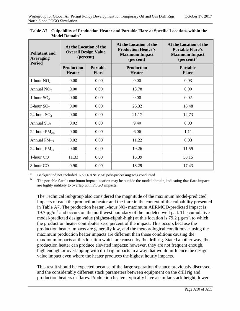
Workgroup for Global Air Permit Policy Development for Temporary Oil and Gas Drill Rigs October 17, 2017
North Slope POGO Simulation
Page A10 of A11
Table A7 Culpability of Production Heater and Portable Flare at Specific Locations within the
Model Domain a
Pollutant and
Averaging
Period
At the Location of the
Overall Design Value
(percent)
At the Location of the
Production Heater’s
Maximum Impact
(percent)
At the Location of the
Portable Flare’s
Maximum Impact
(percent) b
Production
Heater
Portable
Flare
Production
Heater
Portable
Flare
1-hour NO2 0.00 0.00 0.00 0.03
Annual NO2 0.00 0.00 13.78 0.00
1-hour SO2 0.00 0.00 0.00 0.02
3-hour SO2 0.00 0.00 26.32 16.48
24-hour SO2 0.00 0.00 21.17 12.73
Annual SO2 0.02 0.00 9.40 0.03
24-hour PM2.5 0.00 0.00 6.06 1.11
Annual PM2.5 0.02 0.00 11.22 0.03
24-hour PM10 0.00 0.00 19.26 11.59
1-hour CO 11.33 0.00 16.39 53.15
8-hour CO 0.90 0.00 18.29 17.43
a Background not included. No TRANSVAP post-processing was conducted.
b The portable flare’s maximum impact location may be outside the model domain, indicating that flare impacts
are highly unlikely to overlap with POGO impacts.
The Technical Subgroup also considered the magnitude of the maximum model-predicted
impacts of each the production heater and the flare in the context of the culpability presented
in Table A7. The production heater 1-hour NO2 maximum AERMOD-predicted impact is
19.7 µg/m3 and occurs on the northwest boundary of the modeled well pad. The cumulative
model-predicted design value (highest-eighth-high) at this location is 79.2 µg/m3, to which
the production heater contributes zero percent of the impact. This occurs because the
production heater impacts are generally low, and the meteorological conditions causing the
maximum production heater impacts are different than those conditions causing the
maximum impacts at this location which are caused by the drill rig. Stated another way, the
production heater can produce elevated impacts; however, they are not frequent enough,
high enough or overlapping with drill rig impacts in a way that would influence the design
value impact even where the heater produces the highest hourly impacts.
This result should be expected because of the large separation distance previously discussed
and the considerably different stack parameters between equipment on the drill rig and
production heaters or flares. Production heaters typically have a similar stack height, lower

Workgroup for Global Air Permit Policy Development for Temporary Oil and Gas Drill Rigs October 17, 2017
North Slope POGO Simulation
Page A11 of A11
exit temperature and velocity, and larger stack diameter than most equipment on a drill rig.
Portable flares typically have higher effective stack heights, exit temperature, and larger
effective exit diameter than most equipment on a drill rig. In addition, this equipment is
typically not near other structures, and therefore, was not simulated with downwash. These
aspects of the operation of production heaters and flares, as well as separation from other
sources of emissions, keep (1) plumes from overlapping in space and (2) plumes from
overlapping under the same meteorological conditions (in time). With these considerations,
the Technical Subgroup determined that it was not necessary to explicitly include equipment
like production heaters and portable flares in the North Slope POGO Simulation.
Prepared by: AECOM
October 17, 2017
Appendix B
Drill Rig Equipment Inventory Survey

Workgroup for Global Air Permit Policy Development for Temporary Oil and Gas Drill Rigs October 17, 2017
North Slope POGO Simulation
Page B1 of B1
Figure B1 Results of Drill Rig Inventory Survey

Prepared by: AECOM
October 17, 2017
Appendix C
Transportable Source Variability Processor
(TRANSVAP)

Workgroup for Global Air Permit Policy Development for Temporary Oil and Gas Drill Rigs October 17, 2017
North Slope POGO Simulation
Page C1 of C17
C1. INTRODUCTION
Given the stringency of the short-term probabilistic National Ambient Air Quality Standards
(NAAQS) and the need to include non-stationary emissions units (EUs) in NAAQS compliance
demonstrations using steady state dispersion modeling in Alaska, a robust technique was
developed to predict air quality impacts from EUs that are characterized by portable, temporary,
and intermittent operations. Examples of such equipment and operations could include drill rigs,
hydraulic fracturing units and other well servicing activities, rock crushers, asphalt batch plants,
construction equipment, and shipping vessels and other port operations. This technique was
implemented as a post-processor, called the Transportable Source Variability Processor
(TRANSVAP),29
for U.S. Environmental Protection Agency (USEPA) Modeling Guideline30
dispersion models. Because this technique better simulates the transitory nature of portable
sources, it fills a gap in USEPA’s Modeling Guideline and predicts more realistic concentrations
for assessing compliance with the probabilistic and multi-year form of the 1-hour NO2, 1-hour
SO2, and 24-hour PM2.5 NAAQS.
For the North Slope POGO Simulation, the TRANSVAP post-processor was used to more
realistically simulate the transitory nature of a drill rig operating for varying lengths of time at
multiple well locations across a well pad. The following discussion outlines background on the
TRANSVAP post-processor, how inputs are developed for TRANSVAP, and how TRANSVAP
was implemented for the North Slope POGO Simulation.
C2. TRANSVAP BACKGROUND
TRANSVAP was designed to predict a representative distribution of impacts from portable
sources by taking advantage of the fact that these sources: (1) only remain at a location for a
limited period of time, (2) can have a random spatial distribution, and (3) can have various
physical configurations. This technique was implemented as a post-processor that utilizes output
from USEPA Modeling Guideline dispersion models, such as AERMOD and OCD. The models
themselves do not need to be modified for use with TRANSVAP and, therefore, do not constitute
an alternative modeling technique under Section 3.2 of the Guideline. Because TRANSVAP is
model-independent, the technique is flexible enough to be used in short-range and long-range, as
well as over land and over water, applications. TRANSVAP is designed to provide a
conservatively representative distribution of model-predicted impacts from one or more portable
sources operating at locations according to a random or predictable pattern. The resulting
distribution of design values (a distribution describing the probability that a particular impact
will occur in time) is more consistent with describing impacts from portable sources than the
29
Additional information available in TRANSVAP: A new technique for predicting impacts from portable or
transitory sources (Damiana, T.A. and Hamel, R.P., 2013), presented and published through the Air and Waste
Management Association (AWMA) – Guideline on Air Quality Models 2013: The Path Forward Conference in
Raleigh, North Carolina, March 19-21, 2013. 30
USEPA Guideline on Air Quality Models, 40 CFR 51, Appendix W promulgated November 9, 2005. Draft
revisions to the Guideline proposed by USEPA were published in the Federal Register on July 14, 2015, and the
revised Guideline became effective on May 22, 2017. All references to the Guideline in this document refer to
the version in place when the modeling was conducted (November 9, 2005 version). Differences in the
references between the 2005 and 2017 Guidelines are indicated.

Workgroup for Global Air Permit Policy Development for Temporary Oil and Gas Drill Rigs October 17, 2017
North Slope POGO Simulation
Page C2 of C17
results from single model runs because of the unpredictable spatial and temporal nature of
portable sources.
Figure C1 illustrates how the TRANSVAP post-processing technique compares to more
conservative and unrealistic standard modeling approaches for a potential drill rig operation.
Figure C1(a) illustrates the standard conservative modeling approach, assuming a constant drill
rig operation at a single location and at its potential-to-emit or a permitted limit over the entire
modeled period. For this type of operation, this scenario is unrealistic and does not occur. An
alternative to the conservative modeling approach in Figure C1(a) would be modeling the drill
rig operating only during specific periods according to a fixed schedule as depicted in
Figure C1(b). While this scenario is more realistic, this type of modeling demonstration could
lead to impractical permit conditions that hold the drill rig operation to a fixed schedule. While
these activities can be planned in advance, operators almost always need to deviate from their
original drilling plan due to unforeseen circumstances. TRANSVAP provides a solution to this
by processing up to 10,000 different randomly-generated scenarios of possible drill rig activity,
as shown in Figure C1(c). This approach accounts for any number of different operational
scenarios in order to determine a worst-case reality.
C3. OVERVIEW: HOW TRANSVAP WORKS
TRANSVAP was developed as a post-processor that utilizes binary output from AERMOD for
each distinctly identified short-term operational scenario. TRANSVAP uses a series of
realizations designed to represent possible sequences of activity amongst those operational
scenarios to generate modeled design concentrations from thousands of those realizations. The
results are then presented in a statistical manner that can be used to characterize the distribution
of possible air quality impacts from a portable source for use in assessing compliance with the
NAAQS.
C3.1 TRANSVAP Control File
In order to run TRANSVAP, the user must create a TRANSVAP Control File which
provides the program with the following information:
Number of modeled meteorological years and dates within those years to be
analyzed in the study; up to five meteorological years can be specified.
Total number of receptors used in the AERMOD simulation and the filename
containing those receptors.
NAAQS being evaluated; TRANSVAP currently supports 1-hour NO2, 1-hour SO2,
and 24-hour PM2.5 probabilistic NAAQS.
Percentile ranking of design values output from TRANSVAP. Default rankings are
50th
, 60th
, 70th
, 75th
, 80th
, 85th
, 90th
, and 95th
percentiles. Percentile rankings can also
be user-defined.

Workgroup for Global Air Permit Policy Development for Temporary Oil and Gas Drill Rigs October 17, 2017
North Slope POGO Simulation
Page C3 of C17
(a) Continuous Operation - Highly Conservative for Modeling a Portable Source
(b) Intermittent Operation - More Realistic for a Portable Source, but only One of Many
Possibilities
(c) Intermediate Operation - Several Realizations of Operational Profiles using the
TRANSVAP Approach
Figure C1 Potential Modeling Approaches for a Portable and Transitory Operation

Workgroup for Global Air Permit Policy Development for Temporary Oil and Gas Drill Rigs October 17, 2017
North Slope POGO Simulation
Page C4 of C17
Filenames of all of the AERMOD binary files representing impacts generated for
each operational scenario processed with TRANSVAP.
Filenames of all TRANSVAP simulation files for use with TRANSVAP. These files
contain instructions for how to string together series of identified short-term portable
source operational modes into each of the thousands of realizations of activity.
C3.2 TRANSVAP Input Files
Before using TRANSVAP, the user must perform two steps in order to prepare key files
necessary for input into the program. The development of these inputs is discussed in the
following sections.
C3.2.1 AERMOD Binary Files
The user must define a number of operational scenarios that represent distinct short-
term activities of one or more portable sources operating at a given location or multiple
locations either individually or simultaneously. For example, the sources representing a
drilling operation at a location might be considered one operational scenario, while
another operational scenario might represent hydraulic fracturing operations at that
same location, while yet another might be the same drilling equipment as used in the
first scenario but operating at a different load or entirely different location. For each
operational scenario identified by the user, one AERMOD run must be executed and a
binary file of the modeled concentrations in AERMOD’s POSTFILE format (either in
1-hour or 24-hour periods depending on the standard under consideration) generated
containing the results from the entire period of meteorological data being modeled. One
binary file representing each operational scenario will be input into TRANSVAP.
Because this AERMOD run can contain any of the combinations of source types,
emission rates, and source locations that an AERMOD run can contain, there is great
flexibility in the kinds of operational scenarios that TRANSVAP can simulate.
C3.2.2 TRANSVAP Simulation Files
The user must also generate a number of operating schedules, or realizations, which
represent a possible sequence of user developed operational modes over the
meteorological period being modeled. To define each simulation, it is necessary to first
determine the probability distribution for each operational scenario under consideration.
For example, suppose Scenario 1 represents well drilling, while Scenario 2 represents
hydraulic fracturing. Probability distributions for each scenario are developed using
knowledge of how these activities typically occur. For example, using the typical mean
number of days that well drilling occurs, and a typical standard deviation from the
mean, spreadsheet tools can be used to generate a series of random numbers
representing the probable number of hours that well drilling occurs. Similar sets of
random numbers can be generated for hydraulic fracturing and for periods of inactivity
when neither well drilling nor hydraulic fracturing occurs. These numbers are then
combined to define as many realizations as are desired, and are used to produce the
TRANSVAP Simulation File.

Workgroup for Global Air Permit Policy Development for Temporary Oil and Gas Drill Rigs October 17, 2017
North Slope POGO Simulation
Page C5 of C17
The format of the TRANSVAP Simulation File is a list of hours for each simulation at
which the activity of one or more of the operational scenarios starts. During the period
starting with the hour identified, an operational mode that is active is signified by a “1”
for on, or “0” for off. For example, a single simulation representing two operational
scenarios modeled over a five-year period might look like the example below. In this
example shown in Figure C2, for hours 1 through 7,870 both scenarios are set to 0 and
therefore are inactive. At hour 7,871, Scenario 1 becomes active and remains active
through hour 8,230, at which point both scenarios are inactive until hour 13,775 when
Scenario 2 becomes active through hour 14,110 of the five-year period, etc. This
simulation is also shown graphically as a time series of activity in Figure C2(b). There
are no restrictions regarding the number of scenarios that can be active or inactive
simultaneously, or the number of realizations that can be included one after the next in
a single TRANSVAP analysis (depending on computer resources available).
C3.3 Executing TRANSVAP
Once the user creates the necessary files, the TRANSVAP executable must be run based on
the inputs provided by the user in a control file. All of the necessary files are imported into
the program and each simulation outlined in the TRANSVAP Simulation File is run by the
following process:
For each averaging period, dependent on the NAAQS being evaluated, the program
determines if any of the user-defined operational scenarios are active. If they are not,
the modeled concentrations for the period are set to zero.
For any operational scenario that is active during the period (1-hour or 24-hours
depending on the NAAQS evaluated), the modeled concentration for that operational
scenario is summed with the modeled concentrations from any other active
operational scenarios to produce an overall modeled concentration for that period at
each receptor.
Once all hours are processed for a particular simulation period, appropriate design
concentrations are calculated according to the NAAQS being evaluated and then
written to a file.
Once all realizations have been completed, design values for each user specified
percentile rank are calculated and presented to the user.
TRANSVAP produces the following output:
A file containing the design concentrations for each simulation defined in the
TRANSVAP Simulation File, identifying the design concentration and the receptor
at which the design concentration for that simulation occurred.
A violation report file containing a list of every receptor at which the design
concentration exceeded the NAAQS for each simulation defined in the TRANSVAP
Simulation File.

Workgroup for Global Air Permit Policy Development for Temporary Oil and Gas Drill Rigs October 17, 2017
North Slope POGO Simulation
Page C6 of C17
A file containing the modeled concentration, in the form of the standard, at every
receptor for each simulation defined in the TRANSVAP Simulation File.
For every simulation, a file reflecting the activity switches used for that simulation,
taken from the TRANSVAP Simulation File, and the yearly modeled concentrations
for each receptor. These files are primarily for quality assurance and debugging.
Example Format of Simulation:
START SIMULATION 1
**Hour SCENARIO 1 SCENARIO 2
1 0 0
7871 1 0
8231 0 0
13775 0 1
14111 0 0
15623 0 1
16007 0 0
20207 0 1
20495 0 0
23855 0 1
24191 0 0
29567 0 1
29807 0 0
36023 0 1
36431 0 0
41975 0 1
42311 0 0
END SIMULATION 1
Figure C2 Example (a) TRANSVAP Simulation File and (b) Graphical Depiction for a Single
Simulation
(a)
(b)

Workgroup for Global Air Permit Policy Development for Temporary Oil and Gas Drill Rigs October 17, 2017
North Slope POGO Simulation
Page C7 of C17
The TRANSVAP.OUT file provides a statistical analysis based on the results from
each of the realizations defined in the TRANSVAP Simulation File. This file
presents the following information:
o For every receptor, the overall maximum design concentration calculated over
all realizations, the average design concentration calculated over all realizations,
and eight different percentile results of the design values calculated over all
realizations. By default, the program presents, for each receptor, the 50th
, 60th
,
70th
, 75th
, 80th
, 85th
, 90th
, and 95th
percentiles design concentrations over all
realizations. These percentile values are customizable by the user.
o The highest design concentration, highest average value, and highest design
concentration at each of the percentile levels described above is reported
separately.
o For the overall highest design concentration, the receptor at which it occurred
and the simulation it occurred in is identified.
o For the highest overall average design concentration, the receptor at which it
occurred is identified.
o If the NAAQS is violated at any receptor, the percentile result at which the
violation occurred.
C4. APPLICATION OF TRANSVAP FOR THE NORTH SLOPE POGO
SIMULATION
TRANSVAP was used to post-process AERMOD-predicted impacts for 1-hour NO2 and
1-hour SO2 averaging periods for the North Slope POGO Simulation. Sections C4.1 through
C4.4 summarize input development for post-processing the North Slope POGO Simulation with
TRANSVAP. Figure C2 illustrates the AERMOD and TRANSVAP processing steps specific to
the North Slope POGO Simulation. The process outlined would be used for each fuel
consumption modeled.
C4.1 TRANSVAP Control File
As described in Section C3, there are several key inputs required to use the TRANSVAP
post-processor. For the North Slope POGO Simulation, required inputs specified in the
control file are summarized in Table C1 for both the 1-hour NO2 and 1-hour SO2 modeling
demonstrations.
C4.2 Receptor Grid
For computational efficiency, the full AERMOD receptor grid described in the North Slope
POGO Simulation modeling report is refined to only consider receptors with
AERMOD-predicted impacts for a representative fuel consumption that show a violation of
the NAAQS. This processing step was performed for all AERMOD simulations that are
post-processed with TRANSVAP.

Workgroup for Global Air Permit Policy Development for Temporary Oil and Gas Drill Rigs October 17, 2017
North Slope POGO Simulation
Page C8 of C17
C4.3 AERMOD Output
All required AERMOD binary output files were generated in POSTFILE (*.pos) format. A
POSTFILE was generated for each of the six operational scenarios which consist of a drill
rig operating at five different well locations across a representative well pad and one
scenario with no drill rig operation. Modeled drill rig locations across the well pad are
illustrated in Figure C3.
C4.4 TRANSVAP Simulation Files
As previously described, TRANSVAP recombines AERMOD-predicted impacts according
to randomly-generated drill rig realizations. To develop and generate the different
realizations of drill rig activity, a TRANSVAP Simulation File for the North Slope POGO
Simulation, there were three degrees of freedom considered:
Location of the drill rig (See Figure C3).
Duration of active drilling.
Duration without drill rig activity.
Table C1 North Slope POGO Simulation Control File
Pollutant Isolated Pad Collocated Pad
RDi DDi RDc DDc
Meteorological
Years Processed
1-hour NO2 5 years – 2006, 2007, 2008, 2009, 2010
1-hour SO2
Number of
Receptors and
Filename with
Receptors
1-hour NO2 100
(ReGrid_NO2_isolated.dat) 152
(ReGrid_NO2_collocated.dat)
1-hour SO2 100 (ReGrid_SO2.dat)
NAAQS
Evaluated
1-hour NO2 Option 2
1-hour SO2 Option 1
Percentile
Ranking of
Design Values
1-hour NO2
Default (50th
, 60th
, 70th
, 75th
, 80th
, 85th
, 90th
, and 95th
) 1-hour SO2
AERMOD
Output Files for
Each
Operational
Scenario
1-hour NO2
Drill Rig Not Operating at Well Pad: DRILLING_SC1_SO2.POS
Drill Rig Operating at Well Location 2: DRILLING_SC2_SO2.POS
Drill Rig Operating at Well Location 3: DRILLING_SC3_SO2.POS
Drill Rig Operating at Well Location 4: DRILLING_SC4_SO2.POS
Drill Rig Operating at Well Location 5: DRILLING_SC5_SO2.POS
Drill Rig Operating at Well Location 6: DRILLING_SC6_SO2.POS
1-hour SO2
TRANSVAP
Activity Profiles
1-hour NO2 WOA_INFILL_
23-OCT-2014.inp
Rig_Movement_
22-APR-2014.inp
WOA_INFILL_
23-OCT-2014.inp
Rig_Movement_
22-APR-2014.inp 1-hour SO2

Workgroup for Global Air Permit Policy Development for Temporary Oil and Gas Drill Rigs October 17, 2017
North Slope POGO Simulation
Page C9 of C17
Based on these degrees of freedom and actual operational data collected on the North Slope,
10,000 realizations of drill rig activity were developed.
Model-predicted impacts are predicted with AERMOD for each operational scenario, which,
in this case, consists of a drill rig operating at each location at the well pad continuously and
one where the drill rig is not operating at any of the well pad locations. The individual well
site locations are depicted in Figure C3. Model-predicted impacts at each of these locations
are then recombined according to 10,000 different realizations of drill rig activity.
Sections C4.4.1 and C4.4.2 describe the development of the unique activity profiles for
routine infill drilling and developmental drilling activities.
C4.4.1 Routine Infill Drilling Activity
Routine infill drilling is characterized by intermittent drilling at a well pad where the
drill rig operates at a well pad, leaves, and then returns to the well pad to operate after a
period of inactivity. To characterize the activity on the North Slope, an analysis was
conducted on 6.5 years of daily drill rig activity data. This data was collected for drill
rig activities occurring across 26 separate well pads in the Western Operating Area of
the Prudhoe Bay Unit (PBU). The data was analyzed to characterize the duration of
time when a drill rig was operating at a well pad and duration of time when a drill rig
was not operating at a well pad. The information derived from the PBU data are
summarized in the form of probability frequency distributions in Figure C4. For
processing with TRANSVAP, a probability density function is fitted to each of these
datasets. Active drilling activity is characterized by a lognormal probability density
function with a mean of 29.5 days and standard deviation of 34.9 days. Inactivity is
characterized by a gamma probability density function with a mean of 160.1 days and
standard deviation of 200.6 days.
Using these activity and inactivity probability density functions, a TRANSVAP
Simulation File is developed for input into TRANSVAP. To create five years of
intermittent drill rig activity at a well pad for modeling, activity proceeds as follows:
Well pad is vacant between 0 and 365 days.
Drill rig operates at one of the five well locations for a random duration of time
determined according to the lognormal drill rig activity profile.
Drill rig is inactive at the well pad for a random duration of time determined
according to the gamma drill rig inactivity profile.
Alternating drill rig activity and inactivity continue through the remainder of the
five-year modeled period according to the activity and inactivity profiles.
For routine infill drilling, the lognormal probability density function was selected to
better represent the tail of the active drilling dataset that is less representative of routine
infill drilling activities. This type of distribution does not represent typical routine infill
drilling activities, which last between 30 to 60 days, as well as other probability density
functions considered. This has the effect of increasing the likelihood of non-routine

Workgroup for Global Air Permit Policy Development for Temporary Oil and Gas Drill Rigs October 17, 2017
North Slope POGO Simulation
Page C10 of C17
infill drilling activities, such as multi-year drilling events at a single well, occurring
amongst the 10,000 realizations and adding additional conservativism into the analysis.
C4.4.2 Developmental Drilling Activity
Developmental drilling is characterized by continuous drilling at a well pad where a
drill rig moves from one well to another with little to no inactivity between drilling new
wells. To represent developmental drilling activity for the North Slope, a drill rig is
assumed to be operating at one of five well locations for an average of three weeks to
drill a new well before drilling another new well at the well pad. Active drilling activity
is characterized by a normal probability density function with a mean of 21 days and
standard deviation of 3.5 days. This characterization is based on a typical drilling cycle
rather than the PBU data discussed for infill drilling activity. However, because
continuous drilling is assumed, the analysis is not very sensitive to the duration of
activity at any particular well location.
The probability density functions used to represent developmental drilling activity and
inactivity are depicted in Figure C5.
To create five years of developmental drill rig activity at a well pad for modeling,
activity proceeds as the following:
Well pad is vacant between 0 and 730 days (2 years).
Drill rig operates at one of the five well locations for a random duration of time
determined according to the normal drill rig activity profile.
Continuous drill rig activity through the remainder of the five-year modeled
period among the five well locations at the well pad according to the normal drill
rig the activity profile.
Using this characterization, developmental drilling activities are simulated for three to
five years of continuous drilling. The maximum model-predicted impacts are most
likely to occur with realizations of drill rig activity that have the longest period of
continuous drilling activity because of the multi-year average form of the 1-hour
standards. Therefore, this is a very conservative characterization of developmental
drilling because continuous drilling for that length of time on the North Slope is
unrealistic.
C4.5 Using TRANSVAP Results for the North Slope POGO Simulation
For the North Slope POGO Simulation, the 99th
percentile of the distribution of impacts
predicted for the 10,000 realizations of drill rig activity is used to represent design value air
quality impacts for comparison to the NAAQS.

Workgroup for Global Air Permit Policy Development for Temporary Oil and Gas Drill Rigs October 17, 2017
North Slope POGO Simulation
Page C11 of C17
Figure C2 Flowchart of Processing for North Slope POGO Simulation

Workgroup for Global Air Permit Policy Development for Temporary Oil and Gas Drill Rigs October 17, 2017
North Slope POGO Simulation
Page C12 of C17
Figure C3 Configuration of Representative Well pad with Five Modeled Well (Drill Rig) Locations

Workgroup for Global Air Permit Policy Development for Temporary Oil and Gas Drill Rigs October 17, 2017
North Slope POGO Simulation
Page C13 of C17
Figure C4 Representative Routine Infill Drilling Activity Profiles
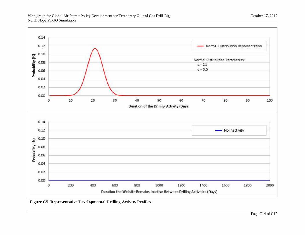
Workgroup for Global Air Permit Policy Development for Temporary Oil and Gas Drill Rigs October 17, 2017
North Slope POGO Simulation
Page C14 of C17
Figure C5 Representative Developmental Drilling Activity Profiles

Workgroup for Global Air Permit Policy Development for Temporary Oil and Gas Drill Rigs October 17, 2017
North Slope POGO Simulation
Page C15 of C17
C5. SENSITIVITY ANALYSIS: STATISTICAL CONVERGENCE OF
THE MODELING
Sensitivity analyses were conducted to show that the results are stable regardless of which set of
10,000 realizations of drill rig activity are selected, and to show that 10,000 realizations is
sufficient to generate a stable result. Two separate analyses were conducted to test the statistical
convergence of TRANSVAP post-processed 1-hour NO2 AERMOD-predicted results by (1)
varying the number of realizations of drill rig activity processed with TRANSVAP and (2)
creating multiple randomly-generated activity input files.
Sensitivity analyses were conducted for 1-hour NO2 modeling for the RDi POGO category with
drill rig operation at 12,000 gallons per day and AERMOD version 14134. While the
representative fuel consumption selected is not important to these analyses, the conclusions of
these analyses are sensitive on the number of and nature of the degrees of freedom incorporated
into the model simulation. Degrees of freedom include well location, duration of drill rig
activity, and duration of drill rig inactivity. These AERMOD runs do not include transient hourly
excursions and do not represent a compliance demonstration for the North Slope POGO
Simulation. Therefore, the model-predicted impacts presented do not have meaning in the
context of the allowable fuel consumption determined for North Slope POGOs.
C5.1 Convergence of Results and the Number of Realizations
Table C2 summarizes 1-hour NO2 results after TRANSVAP post-processing while varying
the number of realizations of drill rig activity processed. Model-predicted impacts indicate
results generally converge with less than 1,000 realizations. The maximum
AERMOD-predicted impacts will continue to vary as additional realizations are processed.
However, the average and other statistical percentile results show little variability beyond
1,000 realizations.
Table C2 1-Hour NO2 Results Varying the Number of Realizations of Drill Rig Activity
Number of
Realizations
of Drill Rig
Activity
Design Concentrations (µg/m3)
Maximum 99
th
Percentile
95th
Percentile
90th
Percentile
75th
Percentile
50th
Percentile Average
100 153.26 146.36 135.86 129.45 119.41 108.53 111.03
500 162.10 148.81 135.77 130.38 121.57 112.04 113.13
1,000 162.10 147.03 137.06 131.26 121.93 112.33 113.38
2,500 162.10 147.03 137.39 131.70 122.07 112.89 113.43
5,000 164.97 147.17 137.17 131.47 122.04 112.79 113.40
7,500 164.97 147.69 137.64 131.74 122.23 112.74 113.50
10,000 164.97 147.74 137.45 131.84 122.39 112.79 113.60

Workgroup for Global Air Permit Policy Development for Temporary Oil and Gas Drill Rigs October 17, 2017
North Slope POGO Simulation
Page C16 of C17
C5.2 Convergence of Results and Randomly-Generated Activity Input Files
Table C3 summarizes 1-hour NO2 results after TRANSVAP post-processing with ten
different randomly-generated TRANSVAP activity input files. Each activity input file was
created with 10,000 realizations of drill rig activity. Model-predicted impacts indicate that
the specific realizations comprising the activity input file made little difference to the
model-predicted impacts. Similar to varying the number of realizations, the most variability
is seen in the maximum results, while the average and other statistical percentile results
show less variability in results.
Table C3 1-Hour NO2 Results Predicted with Different Activity Input Files
File #
Design Concentrations (µg/m3)
Maximum 99
th
Percentile
95th
Percentile
90th
Percentile
75th
Percentile
50th
Percentile Average
1 164.97 147.74 137.45 131.84 122.39 112.79 113.60
2 165.09 147.77 137.25 131.59 122.63 112.43 113.47
3 164.33 147.17 137.23 131.54 122.54 112.60 113.49
4 161.84 147.68 137.15 131.42 122.17 112.45 113.17
5 166.85 147.88 137.43 131.91 122.65 112.64 113.50
6 171.37 147.64 137.28 131.96 122.94 112.96 113.68
7 169.80 147.16 137.27 131.63 122.55 112.89 113.53
8 166.50 146.39 136.89 131.57 122.48 112.72 113.43
9 165.93 147.64 137.72 132.14 122.74 112.90 113.69
10 162.53 147.70 137.35 131.76 122.69 112.82 113.55
Summary
Minimum 161.84 146.39 136.89 131.42 122.17 112.43 113.17
Maximum 171.37 147.88 137.72 132.14 122.94 112.96 113.69
Range 9.53 1.49 0.83 0.72 0.77 0.53 0.52
Average 165.92 147.48 137.30 131.74 122.58 112.72 113.51
Std. Dev. 2.95 0.45 0.22 0.22 0.21 0.19 0.15
C5.3 Conclusions
The following conclusions can be drawn from the two sensitivity analyses conducted with
the TRANSVAP post-processor. TRANSVAP post-processing with 10,000 realizations of
drill rig activity is sufficient:
to allow for the convergence of results.
to account for the expected variability in randomly-generated drill rig activity.

Workgroup for Global Air Permit Policy Development for Temporary Oil and Gas Drill Rigs October 17, 2017
North Slope POGO Simulation
Page C17 of C17
to capture a diverse range of realizations of drill rig activity, such that one set of
10,000 realizations produces identical results to an independently produced set or
realizations.
For the North Slope POGO Simulation, these sensitivity analyses demonstrate the approach
is robust. This analysis also supports using the 99th
percentile TRANSVAP-processed
results to evaluate impacts from North Slope POGOs. Based on the sensitivity analyses
conducted, the 99th
percentile results show better general convergence and less variability in
results than that maximum.
Sensitivity analyses were not conducted for a developmental drilling, DDi or DDc, POGO
categories because the developmental drilling activity input files have fewer degrees of
freedom and will have less variability than routine infill drilling results.

Prepared by: AECOM
October 17, 2017
Appendix D
Second Tier Approach to Combining Model-Predicted Impacts
with a Monitored NO2 Background

Workgroup for Global Air Permit Policy Development for Temporary Oil and Gas Drill Rigs October 17, 2017
North Slope POGO Simulation
Page D1 of D8
D1. INTRODUCTION
Guidance published by the U.S. Environmental Protection Agency (USEPA) offers multiple
approaches for developing monitored 1-hour NO2 background concentrations to combine with
model-predicted impacts. Given the stringency of the 1-hour NO2 National Ambient Air Quality
Standard (NAAQS), a second tier approach was used to combine background concentrations
with model-predicted impacts from the North Slope POGO Simulation. This appendix reviews
the development and implementation of a second tier 1-hour NO2 background approach using
data collected at representative North Slope monitoring stations. The representativeness of the
monitored data collected at these stations is discussed in the modeling report for the North Slope
POGO Simulation.
D2. BACKGROUND
A guidance memo published by the USEPA31
outlines a tiered approach to develop monitored
NO2 background values to assess compliance with the 1-hour NO2 National Ambient Air Quality
Standard (NAAQS). The first tier approach assumes “a uniform monitored background
contribution” by “[adding] the overall highest hourly background NO2 concentration (across the
most recent three years) from a representative monitor to the modeled design value.” A less
conservative first tier approach assumes “a uniform monitored background contribution based on
the monitored design value” (98th
percentile of the annual distribution of daily maximum 1-hour
values). Though these approaches are generally acceptable, the first tier approach may “be overly
conservative in many cases and may also be prone to reflecting source-oriented impacts from
nearby sources.”31
USEPA also provides guidance on a second tier approach that can be used if a first tier approach
is overly conservative and compliance cannot be demonstrated with that approach. The second
tier approach is a collection of approaches that involves developing background concentrations
based on identifying “the meteorological conditions accompanying the concentrations of
concern”32
(meteorological conditions of concern). For sources with diurnal patterns of ambient
impacts, USEPA suggests a temporally varying background based on “multiyear averages of the
98th-percentile of the available background concentrations by season and hour-of-day, excluding
periods when the source in question is expected to impact the monitored concentration.”31
When
identifying meteorological conditions of concern, the second tier approach can also be
interpreted to include methods in which the monitored NO2 background levels can be shown to
vary by wind direction, wind speed, hour of day, day of week, or month of year, as appropriate.
Second tier approaches are representative because “the monitored values will be temporally
paired with modeled concentrations based on temporal factors that are associated with the
31
USEPA Memorandum from Tyler Fox to Regional Air Division Directors, Additional Clarification Regarding
Application of Appendix W Modeling Guidance for the 1-hour NO2 National Ambient Air Quality Standard,
dated March 1, 2011. 32
USEPA Guideline on Air Quality Models, 40 CFR 51, Appendix W promulgated November 9, 2005. Draft
revisions to the Guideline proposed by USEPA were published in the Federal Register on July 14, 2015, and the
revised Guideline became effective on May 22, 2017. All references to the Guideline in this document refer to
the version in place when the modeling was conducted (November 9, 2005 version). Differences in the
references between the 2005 and 2017 Guidelines are indicated.

Workgroup for Global Air Permit Policy Development for Temporary Oil and Gas Drill Rigs October 17, 2017
North Slope POGO Simulation
Page D2 of D8
meteorological variability, but will also reflect worst-case meteorological conditions in a manner
that is consistent with the probabilistic form of the 1-hour NO2 standard.”31
An analysis of NO2 data from the A-Pad and CD1 monitoring stations demonstrated that the
measured 1-hour NO2 concentrations have a strong dependence on wind speed on the North
Slope. This relationship exists because higher wind speeds promote increased dispersion and
dilution of plumes, making NO2 concentrations generally decrease with increasing wind speeds.
Figure D1 illustrates the relationship between hourly average NO2 concentration and hourly
average wind speed measurements at the (a) A-Pad Monitoring Station and (b) CD1 Monitoring
Station. Note that the NO2 concentrations collected at the CD1 Monitoring Station are paired
with wind speed measurements collected at the Nuiqsut Monitoring Station also operated by
ConocoPhillips Alaska, Inc. (CPAI). The Nuiqsut Monitoring Station is located approximately
13 kilometers south of the CD1 Monitoring Station.
Figure D1 clearly shows that the monitored NO2 concentrations at these locations decrease with
increasing wind speed. Therefore, in this case, low wind speeds are associated with the highest
concentrations and are the “meteorological conditions accompanying the concentrations of
concern” referenced in the USEPA guidance. The existence of the relationship shown in
Figure D1 makes a second tier approach appropriate for development of background
concentrations varying by wind speed.
D3. IMPLEMENTATION OF A SECOND TIER APPROACH
The second tier approach for 1-hour NO2 background development is applied using the following
ambient NO2 and wind speed measurements:
A-Pad Monitoring Station data collected between January 1, 2008 and
December 31, 2012(5 years).
CD1 Monitoring Station data collected between October 1, 2012 and September 30, 2014
(2 years).
Background concentrations are determined by first sorting all hourly average NO2 measurements
according to the accompanying wind speed using the categories listed in Table D1. These wind
speed categories are defined in the AERMOD User’s Guide.33
Once the data have been sorted,
the 98th
percentile hourly average NO2 concentration is calculated from the data in each wind
speed category for each year of data. All annual 98th
percentile values are then averaged together
for each wind speed categories. The use of multi-year average monitored background
concentrations accounting for the meteorological conditions of concern is consistent with the
language in USEPA’s Guideline32
and other guidance on modeling for the 1-hour NO2
NAAQS.31
Table D1 summarizes the resulting NO2 background concentrations that were calculated using
data collected at the A-Pad and CD1 monitoring stations. The background NO2 values
33
User’s Guide for the AMS/EPA Regulatory Model – AERMOD (EPA-454/B-03-001), Office of Air Quality
Planning and Standards; September 2004.

Workgroup for Global Air Permit Policy Development for Temporary Oil and Gas Drill Rigs October 17, 2017
North Slope POGO Simulation
Page D3 of D8
corresponding to specific wind speed categories vary from 16.7 to 50.3 µg/m3 using the A-Pad
dataset and from 41.8 to 83.7 µg/m3
using the CD1 dataset.
Once the second tier approach background concentrations are determined, these values are
incorporated into the AERMOD modeling using the “BACKGRND” keyword on the “SO”
pathway and the secondary keyword “WSPEED.” The wind speed categories can be user-defined
by using the “WINDCATS” keyword on the “ME” pathway, though this is unnecessary as
AERMOD default wind speed categories have been used in this analysis. Using this approach,
within the AERMOD run an NO2 background concentration is assigned to all receptors for each
hour of the meteorological input, with the selected background value being determined by the
wind speed for that hour in accordance with Table D1.
D3.1 Data Completeness
Table D2 summarizes the annual and quarterly data completeness for applicable data
collected at the A-Pad Monitoring Station between January 1, 2008 and December 31, 2012.
Table D3 summarizes the annual and quarterly data completeness for applicable data
collected at the CD1 and Nuiqsut monitoring stations between October 1, 2012 and
September 30, 2014. Hourly wind speed data from the A-Pad and Nuiqsut monitoring
stations used in the implementation of the second tier approach meet minimum data
completeness requirements for PSD-quality ambient air quality data. Hourly NO2 data used
to develop background concentrations from the A-Pad and CD1 monitoring stations also
meet minimum PSD data completeness requirements, except for the third quarter of 2008
A-Pad NO2 data. Although this is the case, little bias is expected in the development of
background concentrations because ambient NO2 on the North Slope has no discernible
seasonal variability. Any effect is also minimized by the use of five years rather than three
years of ambient data.
For implementation of the second tier approach, hourly NO2 measurements in the dataset
without a corresponding wind speed measurement were disregarded in the development of
background concentrations. However, given that both parameters generally meet PSD data
completeness requirements and wind speed data completeness is generally very high, near
100 percent, the joint data completeness of these parameters would be similar to the NO2
data completeness, and the joint data completeness was not further analyzed. Any effect on
the calculated background values is also minimized by the use of five years rather than three
years of ambient data.

Workgroup for Global Air Permit Policy Development for Temporary Oil and Gas Drill Rigs October 17, 2017
North Slope POGO Simulation
Page D4 of D8
Figure D1 Relationship Between Hourly NO2 Concentrations and Wind Speed Measured at the
(a) A-Pad and (b) CD1 Monitoring Stations
0
20
40
60
80
100
120
140
160
180
0 2 4 6 8 10 12 14 16 18 20 22 24 26 28 30
NO
2 C
on
cen
trat
ion
(µ
g/m
3)
Wind Speed (m/s)
0
20
40
60
80
100
120
140
160
180
0 2 4 6 8 10 12 14 16 18 20 22 24 26 28 30
NO
2 C
on
cen
trat
ion
(µ
g/m
3 )
Wind Speed (m/s)
CD1 (Collocated Pad) Monitoring Station October 1, 2012 – September 30, 2014
A-Pad (Isolated Pad) Monitoring Station January 1, 2008 – December 31, 2012
(a)
(b)

Workgroup for Global Air Permit Policy Development for Temporary Oil and Gas Drill Rigs October 17, 2017
North Slope POGO Simulation
Page D5 of D8
Table D1 1-Hour NO2 Background Varying by Wind Speed
Wind Speed (WS)
Category a
(m/s)
NO2 Concentration
A-Pad (Isolated Pad) CD1 (Collocated)
(ppbv) (µg/m3) (ppbv) (µg/m
3)
WS < 1.54 26.7 50.3 44.5 83.7
1.54 ≤ WS < 3.09 24.6 46.2 37.0 69.5
3.09 ≤ WS < 5.14 17.0 31.9 30.4 57.2
5.14 ≤ WS < 8.23 12.3 23.2 23.0 43.2
8.23 ≤ WS < 10.8 8.9 16.7 22.2 41.8
WS ≥ 10.8 13.6 25.5 22.6 42.5
a AERMOD-default wind speed categories.

Workgroup for Global Air Permit Policy Development for Temporary Oil and Gas Drill Rigs October 17, 2017
North Slope POGO Simulation
Page D6 of D8
Table D2 Summary of Quarterly and Annual Data Completeness for Hourly NO2 and Wind Speed Measurements at A-Pad (percent)
Data Period
2008 2009 2010 2011 2012
NO2 a
Wind
Speed b
NO2 a
Wind
Speed b
NO2 a
Wind
Speed b
NO2 a
Wind
Speed b
NO2 a
Wind
Speed b
First Quarter (Q1) 91 99 98 100 91 100 96 100 98 96
Second Quarter (Q2) 84 98 97 98 98 97 93 97 92 99
Third Quarter (Q3) 55 99 97 99 98 100 96 99 97 100
Fourth Quarter (Q4) 97 91 98 91 93 100 98 100 98 99
Annual 82 97 97 97 95 99 98 99 96 98
a Hourly NO2 data for all quarters, except third quarter 2008, meet the 80 percent completeness requirement for PSD-quality ambient air quality data.
b Hourly wind speed data for all quarters meet the 90 percent completeness requirement for PSD-quality meteorological data.
Table D3 Summary of Quarterly and Annual Data Completeness for Hourly NO2 Measurements at CD1 Paired with Wind Speed
Measurements at Nuiqsut (percent)
Data Period October 1, 2012 – September 30, 2013 October 1, 2013 – September 30, 2014
NO2 a Wind Speed
b NO2
a Wind Speed
b
First Quarter (Q1) 93 90 97 90
Second Quarter (Q2) 96 95 98 99
Third Quarter (Q3) 96 100 87 97
Fourth Quarter (Q4) 96 100 98 100
Annual 95 96 95 97
a Hourly NO2 data for all quarters meet the 80 percent completeness requirement for PSD-quality ambient air quality data.
b Hourly wind speed data for all quarters meet the 90 percent completeness requirement for PSD-quality meteorological data.
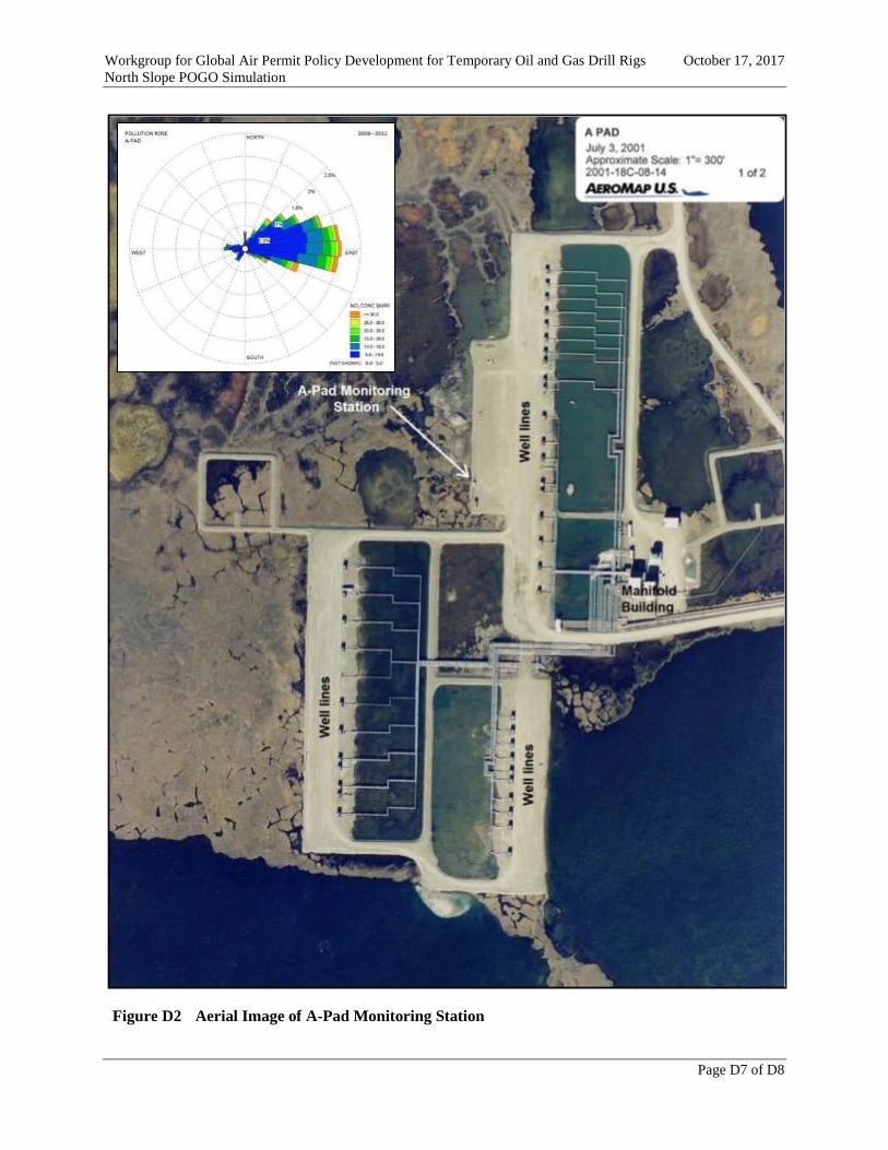
Workgroup for Global Air Permit Policy Development for Temporary Oil and Gas Drill Rigs October 17, 2017
North Slope POGO Simulation
Page D7 of D8
Figure D2 Aerial Image of A-Pad Monitoring Station
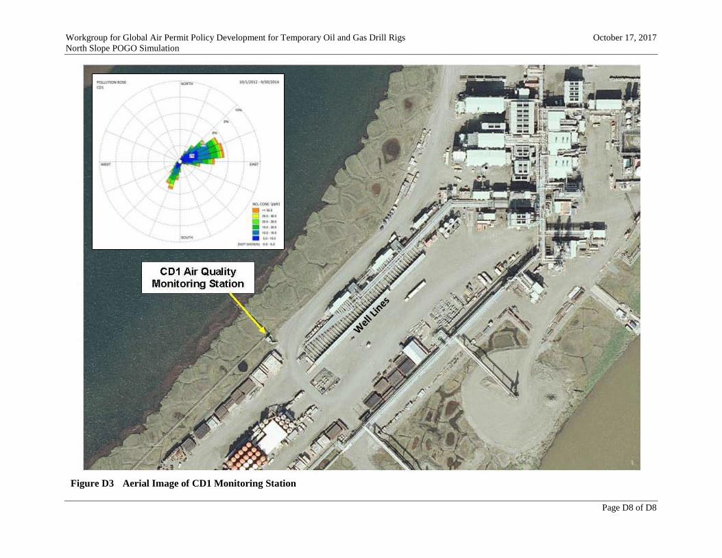
Workgroup for Global Air Permit Policy Development for Temporary Oil and Gas Drill Rigs October 17, 2017
North Slope POGO Simulation
Page D8 of D8
Figure D3 Aerial Image of CD1 Monitoring Station
Prepared by: AECOM
October 17, 2017
Appendix E
Hydraulic Fracturing in Alaska

Workgroup for Global Air Permit Policy Development for Temporary Oil and Gas Drill Rigs October 17, 2017
North Slope POGO Simulation
Page E1 of E7
EXECUTIVE SUMMARY
The purpose of this document is to describe hydraulic fracturing in Alaska for the purpose of
applying ambient air quality background measurements with air quality dispersion modeling.
Hydraulic fracturing, as it’s been conducted in Alaska to date, is captured by the ambient air
quality measurements at several North Slope drill sites. The hydraulic fracturing conducted to
date in Alaska is fracturing of wells drilled for conventional resources, rather than
unconventional. Conventional oil and gas resources are found in more permeable formations
(sandstone) and are easier to produce as oil and gas flow readily to wellbores. Unconventional
resources are found in less permeable formations (shale) and require more energy to produce.
Impacts from hydraulic fracturing of unconventional resources are not captured in existing
ambient air quality measurements because unconventional resources have not yet been brought
into production in Alaska.
E1. INTRODUCTION
The following is a brief discussion characterizing hydraulic fracturing currently occurring in
Alaska and contrasting that with hydraulic fracturing associated with unconventional oil and gas
development which has recently gained significant attention in the lower 48 states. This
discussion is supplemented by a description of current trends and what might be expected in the
future regarding the use of hydraulic fracturing in the development of oil and gas in resources in
Alaska. This discussion relies heavily on North Slope data but is applicable to other parts of
Alaska, as well.
E2. HISTORIAL PERSPECTIVE ON THE PURPOSE OF HYDRUALIC
FRACTURING
Hydraulic fracturing was first conducted in the 1940’s to enhance oil and gas well productivity.
The method was based on the idea that creating fractures or conduits enables fluids to flow more
easily to the wellbore. Since its development, hydraulic fracturing has been used to enhance the
productivity of low permeability formations, remove near-wellbore formation damage caused by
drilling or completion, increase secondary recovery productivity, and increase the capacity of
disposal injection wells (Howard and Fast 1970). In addition to these uses of fracturing, the
method evolved in the 1970s to enable the commerciality of very low permeability “tight” gas
sands. From the 1980s to present, multi stage hydraulic fracturing was combined with horizontal
drilling technology to produce oil and gas from extremely low permeability rocks, such as shales.
This unconventional oil and gas development has led to increased visibility on the role of
hydraulic fracturing.
E3. HISTORIAL PERSPECTIVE ON THE PURPOSE OF HYDRUALIC
FRACTURING
In order to understand how hydraulic fracturing has become a highly visible activity in the past
decade, it is important to understand the difference between conventional and unconventional oil
and gas resources. According to the U.S. Department of Energy (USDOE n.d.):

Workgroup for Global Air Permit Policy Development for Temporary Oil and Gas Drill Rigs October 17, 2017
North Slope POGO Simulation
Page E2 of E7
“Unconventional oil and gas is differentiated from conventional hydrocarbon
resources based on the state of the hydrocarbon, nature of the geologic reservoirs
and the types of technologies required to extract the hydrocarbon. Conventional
oil and gas deposits have a well-defined areal extent, the reservoirs are porous and
permeable, the hydrocarbon is produced easily through a wellbore, and reservoirs
generally do not require extensive well stimulation to produce. Unconventional
hydrocarbon deposits … in general are often lower in resource concentration,
dispersed over large areas, and require well stimulation or additional extraction or
conversion technology. They also are often more expensive to develop per unit of
energy and require a higher price to be economic.”
Oil and gas produced from shale are considered unconventional resources where hydraulic
fracturing is integral to their recovery.
While there are many factors that influence the purpose and design of hydraulic fracturing, there
are a couple of major differences between fracturing conventional and unconventional reservoirs
due to the following factors:
Fracture Gradient: The fracture gradient is “the pressure required to induce fractures in rock
at a given depth.” (Schlumberger 2017). The fracture gradient is stated in pounds per square
inch per foot (psi/ft) or kilo Pascals per meter (kPa/m).
Fracture Half-Length: Fracture half-length is the radial distance from the wellbore to the
limit of fractures created by hydraulic fracturing.
In general, shales have higher fracture gradients than sandstone (Leach 1994) formations. The
significantly higher fracture gradients and fracture half-lengths required for unconventional shale
development leads to very different scales of activities between Alaska and the lower 48 states,
as shown in Table E1. In general, hydraulic fracturing of shale requires more fluid, proppant,
pumping equipment, pumping pressure, and time. Figure E1depicts two hydraulic fracturing
operations at conventional developments on the North Slope. Figure E2 depicts a hydraulic
fracturing operation at an unconventional Woodford Shale development in the lower 48 states.
E4. HYDRAULIC FRACTURING IN ALASKA
The oil and gas resources that are currently being extracted in Alaska are considered
conventional. However, hydraulic fracturing has been an integral part of Alaskan oil production
by increasing the recovery of oil and gas resources. Due to the scale and historical timeline of the
development, the largest body of research comes from North Slope experience. In the mid-1980s,
the operators of Prudhoe Bay noticed a sharp production decline in many wells that was due to
extensive formation damage in the Ivishak formation (Reimers, et al. 1991). Formation damage
typically results from exposing a virgin formation to water, drilling fluids, solids, cement, as well
as damage caused by perforations, which decreases porosity and effective permeability in the
near-wellbore region. Ivishak formation wells that were fractured had production gains averaging
1,600 stock tank barrels per day (STB/D) with gains as high as 5,000 STB/D recorded. In the
stimulation program described by Reimers, et al. (1991), over 100 wells were stimulated
resulting in a production increase of 100,000 STB/D. Hydraulic fracturing also was used to great

Workgroup for Global Air Permit Policy Development for Temporary Oil and Gas Drill Rigs October 17, 2017
North Slope POGO Simulation
Page E3 of E7
Table E1 Comparison of Hydraulic Fracturing Activities for Conventional and
Unconventional Development
Characteristic Alaskan North Slope
Conventional Development a
Unconventional Shale (Tight
Oil or Gas) Development b
Formation Sandstone Shale
Fracture Gradient Low High
Fracture Half Length Short Long
Generally Required for
Resource Recovery
No
(increases flow rate) Yes
Type of Chemicals Will vary depending on reservoir properties and well conditions
Fluid Used (bbls) Less than 30,000 Approximately 300,000+
Proppant (ton) – untreated sands,
ceramics, resin coated sands, etc. Less than 2,000 Approximately 2,000-8,000+
Percent of Wells Fractured Approximately 25 100
Horizontal Well Spacing (ft) 1,200 – 1,500 Approximately 600
Duration of a Fracturing Event
(Engine Operation)
Approximately 1 day
(only 2-3 hours at high load)
Approximately 2-7 days
(varying hours at high load)
Treating Pressure (psi) 5,000 – 8,000 8,500+
Pumping Horsepower (hp) 3,000 16,700
a Review of records from the Kuparuk River Unit and Colville River Unit.
b Review of records from the Denver-Julesburg Basin.

Workgroup for Global Air Permit Policy Development for Temporary Oil and Gas Drill Rigs October 17, 2017
North Slope POGO Simulation
Page E4 of E7
Figure E1 Alaskan North Slope Hydraulic Fracturing with Conventional Developments
3.13.2.1
Figure E2 Hydraulic Fracturing with Unconventional Shale Development
Colville River Unit, CD5 Colville River Unit,
CD3
Provided by ConocoPhillips Alaska, Inc.
A Woodford Shale Development
https://wellworc.com/wp-content/uploads/2016/03/1_Frac.jpg

Workgroup for Global Air Permit Policy Development for Temporary Oil and Gas Drill Rigs October 17, 2017
North Slope POGO Simulation
Page E5 of E7
extent at the Kuparuk field because the “A” sand reservoir was extremely susceptible to damage
from drilling and completion (Niemeyer and Reinart 1986). In the 1980s, an aggressive
fracturing program was implemented using a variety materials and methods in order to determine
optimum stimulation. The fracturing program yielded production gains averaging 300 percent.
Hydraulic fracturing of conventional resources intended to counter formation damage has been a
successful well stimulation technology at North Slope oil and gas fields, and an important factor
in maximizing recovery. It is reported that 25 percent of the oil and gas wells in Alaska have
been stimulated by hydraulic fracturing (Bond 2016).
In recent years, there has been interest in the unconventional resources in source rock shales of
the North Slope. The shale formations include the Triassic Shublik Formation, Jurassic–Lower
Cretaceous Kingak Shale, and Cretaceous pebble shale unit and Hue Shale, referred to as the
Brookian Shale. The U.S. Geological Survey conducted a probabilistic oil and gas resource
assessment that indicated a mean total resource for all the shales as 940 million barrels of oil, 42
trillion cubic feet of gas, and 262 million barrels of natural gas liquids are technically
recoverable from the shales (Houseknecht, et al. 2012). One oil company, Great Bear Petroleum
Operating, LLC (Great Bear), undertook exploration for shale resources on the North Slope in
2010 (Bailey 2016a). Great Bear drilled a couple of wells and conducted extensive testing but
has since decided to explore conventional targets.
E5. CURRENT TRENDS
While the possibility of unconventional resources exists in the Cook Inlet (Schenk, et al. 2015),
discussions have been, and will continue to focus on Alaskan North Slope resources due the
known availability and location of source rock. Shale production on the North Slope is not
limited by whether these shales could yield oil, but rather, if the need for fracturing is cost
prohibitive for commercial production. Successful unconventional shale production is not only
very price sensitive, but also requires a logistical train that will assure adequate supplies of
proppant (silica sand), drilling equipment, fuel, cement, and other necessary commodities (Metz
2013). As alluded to in Table E1, the major difference in the hydraulic fracturing described for
conventional North Slope resources and shale development is the amount of material that would
be needed to stimulate shale wells and the increased number wells to develop a similar area. In
the well stimulation program described by Reimers and Clausen (1991) for Prudhoe Bay, a
typical frac job consumed less than 20 tons of proppant (one bulk truck load) and 900 barrels of
fluid. By contrast, based on Eagle Ford Formation (South Texas) development, a typical well in
the Shublik Formation shale may require up to 6,000 tons (240 bulk truck loads) of proppant and
200,000 to 300,000 barrels of fluid (Metz 2013; LaFollette, et al. 2014). Assuming 200 potential
horizontal shale wells per year (as envisioned by Great Bear), the water and proppant needed
presents an substantial supply chain task. This, in addition to the supply chain issues for drilling
unconventional resources, may explain why Alaska shale resources have been slow to develop
(Hobson 2013).
The issues challenging unconventional shale production in Alaska do not apply to the use of
hydraulic fracturing combined with horizontal wells to develop conventional resources in Alaska
into the future. At Cook Inlet, BlueCrest Alaska Operating, LLC has commenced a program to
drill horizontal wells and conduct staged hydraulic fracturing to enhance recovery from

Workgroup for Global Air Permit Policy Development for Temporary Oil and Gas Drill Rigs October 17, 2017
North Slope POGO Simulation
Page E6 of E7
conventional reservoirs as opposed to unconventional shale (Bailey 2016b). The total amount of
frac fluid that would be used by BlueCrest probably would not exceed 36,000 barrels per well, a
much smaller hydraulic fracturing effort as compared to a “typical” shale well. Recent large
discoveries (Pikka Unit and Smith Bay) in lower permeability Cretaceous rocks on the North
Slope indicate that hydraulic fracturing may be a well stimulation method that will continue to be
used for many years into the future to develop Alaskan conventional oil and gas resources.
E6. REFERENCES
American Oil and Gas Historical Society [AOGHS]. 2017. Shooters – A “Fracking” History.
http://aoghs.org/technology/shooters-well-fracking-history/.
Bailey, A. 2016a. Great Bear Evaluating Eight Prospects: Petroleum News, Volume 21, No. 41,
October 9, 2016. http://petroleumnews.com. Accessed March 12, 2017.
Bailey, A. 2016b. BlueCrest Drilling Ahead: Petroleum News, Volume 21, No. 50, December
11, 2016. . http://petroleumnews.com. Accessed March 12, 2017.
Bond, A. 2016. Fracturing Overview: Fact vs. Fiction. Caelus Energy Alaska, December 8, 2016.
Brehmer, Elwood. 2016. Partners will drill at Icewine in 2017: Alaska Journal of Commerce,
October Issue 1-2016. Wed, 09/28/2016 - 2:09pm.
Hobson, M.K. 2013. Geologist’s Alaska gamble could turn into America’s next big shale play:
E&E News, Energywire, April 3, 2013. https://www.eenews.net/stories/1059978794.
Accessed June 6, 2017.
Houseknecht, D.W., W.A. Rouse, C.P. Garrity, K.J. Whidden, J.A. Dumoulin, C.J. Schenk, R.
Charpentier, T.A. Cook, S.B. Gaswirth, M.A. Kirschbaum, and R.M. Pollastro. 2012.
Assessment of Potential Oil and Gas Resources in Source Rocks of the Alaska North Slope,
2012. U.S. Geological Survey Fact Sheet 2012–3013, February 2012.
Howard, G.C. and C.R. Fast. 1970. Hydraulic Fracturing: Society of Petroleum Engineers of
AIME, Monograph Volume 2 of the Henry A. Doherty Series, 203 p.
LaFollette, R.F., G. Izadi, and M. Zhong. 2014. Application of Multivariate Statistical Modeling
and Geographic Information Systems Pattern-Recognition Analysis to Production Results
in the Eagle Ford Formation of South Texas. Society of Petroleum Engineers paper SPE
168628. The paper was prepared for presentation at the SPE Hydraulic Fracturing
Technology Conference, The Woodlands, Texas, February 4-6, 2014.
Leach, W.G. 1994. Distributions of Hydrocarbons in Abnormal Pressure in South Louisiana,
U.S.A., in Fertl, W.H., R.E. Chapman, and R.F. Hotz, editors, Studies in Abnormal
Pressures. Developments in Petroleum Science 38. Elsivier Science, B.V., Amsterdam,
Netherlands, p. 391 to 428.

Workgroup for Global Air Permit Policy Development for Temporary Oil and Gas Drill Rigs October 17, 2017
North Slope POGO Simulation
Page E7 of E7
Lidji, A. 2017. Icewine Exploration Plan Approved: Petroleum News, Volume 22, No. 1.
http://petroleumnews.com. Accessed March 17, 2017.
Metz, P. 2013. Economic Impact of a North Slope Rail Extension on Future Northern Energy
and Mineral Development.
Niemeyer, B.L. and M.R. Reinart. 1986. Hydraulic Fracturing of a Moderate Permeability
Reservoir, Kuparuk River Unit: Society of Petroleum Engineers paper SPE15507. The
paper was prepared for the 61st Annual Technical Conference and Exhibition, New
Orleans, Louisiana, October 5-8, 1986.
Reimers, D.R., and R.A. Clausen. 1991. High-Permeability Fracturing at Prudhoe Bay, Alaska:
Society of Petroleum Engineers paper SPE 22835. Paper was prepared for the 66th Annual
Technical Conference and Exhibition, Dallas, Texas, October 6-9, 1991, p. 181-194.
Schenk, C.J., and Nelson, P.H., 2015, Geologic model and assessment of potential
unconventional (tight) gas resources in Upper Cook Inlet Basin, South-central Alaska,
chap. 1 of Assessment of unconventional (tight) gas resources in Upper Cook Inlet Basin,
South-central Alaska: U.S Geological Survey Digital Data Series 69–AA, 31 p.,
http://dx.doi.org/10.3133/ds69AA.
Schlumberger. 2017. Oil Field Glossary. Internet website:
http://www.glossary.oilfield.slb.com/Terms/f/fracture_gradient.aspx. Site accessed April 5,
2017.
U.S. Department of Energy (USDOE). Unconventional Energy Resources.
http://www.unconventionalenergyresources.com/#about. Accessed March 16, 2017.