normalized least-squares estimation in time-varying …suhasini/papers/nls08.pdfestimation in...

The Annals of Statistics2008, Vol. 36, No. 2, 742–786DOI: 10.1214/07-AOS510© Institute of Mathematical Statistics, 2008

NORMALIZED LEAST-SQUARES ESTIMATION IN TIME-VARYINGARCH MODELS

BY PIOTR FRYZLEWICZ,1 THEOFANIS SAPATINAS

AND SUHASINI SUBBA RAO2

University of Bristol, University of Cyprusand Texas A&M University

We investigate the time-varying ARCH (tvARCH) process. It is shownthat it can be used to describe the slow decay of the sample autocorrelationsof the squared returns often observed in financial time series, which warrantsthe further study of parameter estimation methods for the model.

Since the parameters are changing over time, a successful estimator needsto perform well for small samples. We propose a kernel normalized-least-squares (kernel-NLS) estimator which has a closed form, and thus outper-forms the previously proposed kernel quasi-maximum likelihood (kernel-QML) estimator for small samples. The kernel-NLS estimator is simple,works under mild moment assumptions and avoids some of the parameterspace restrictions imposed by the kernel-QML estimator. Theoretical evi-dence shows that the kernel-NLS estimator has the same rate of convergenceas the kernel-QML estimator. Due to the kernel-NLS estimator’s ease of com-putation, computationally intensive procedures can be used. A prediction-based cross-validation method is proposed for selecting the bandwidth ofthe kernel-NLS estimator. Also, we use a residual-based bootstrap schemeto bootstrap the tvARCH process. The bootstrap sample is used to obtainpointwise confidence intervals for the kernel-NLS estimator. It is shown thatdistributions of the estimator using the bootstrap and the “true” tvARCH es-timator asymptotically coincide.

We illustrate our estimation method on a variety of currency exchange andstock index data for which we obtain both good fits to the data and accurateforecasts.

1. Introduction. Among models for log-returns Xt = log(Pt/Pt−1) on spec-ulative prices Pt (such as currency exchange rates, share prices, stock indices, etc.),the stationary ARCH(p) [Engle (1982)] and GARCH(p, q) [Bollerslev (1986) andTaylor (1986)] processes have gained particular popularity and have become stan-dard in the financial econometrics literature as they model well the volatility offinancial markets over short periods of time. For a review of recent advances on

Received June 2007; revised June 2007.1Supported in part by the Department of Mathematics, Imperial College, UK.2Supported by the DFG (DA 187/12-2).AMS 2000 subject classifications. Primary 62M10; secondary 62P20.Key words and phrases. Cross-validation, (G)ARCH models, kernel smoothing, least-squares es-

timation, locally stationary models.

742

http://www.imstat.org/aos/

http://dx.doi.org/10.1214/07-AOS510

http://www.imstat.org

http://www.ams.org/msc/

ESTIMATION IN TIME-VARYING ARCH MODELS 743

those and related models, we refer the reader to Fan and Yao (2003) and Giraitis,Leipus and Surgailis (2005).

The modeling of financial data using nonstationary time series models has re-cently attracted considerable attention. Arguments for using such models were laidout, for example, in Fan, Jiang, Zhang and Zhou (2003), Mikosch and Starica(2000, 2003, 2004), Mercurio and Spokoiny (2004a, 2004b), Starica and Granger(2005) and Fryzlewicz et al. (2006).

Recently, Dahlhaus and Subba Rao (2006) generalized the class of ARCH(p)

processes to include processes whose parameters were allowed to change “slowly”through time. The resulting model, called the time-varying ARCH(p)

[tvARCH(p)] process, is defined as

Xt,N = σt,NZt , σ 2t,N = a0

(t

N

)+

p∑j=1

aj

(t

N

)X2

t−j,N ,(1)

for t = 1,2, . . . ,N , where {Zt }t are independent and identically distributed ran-dom variables with E(Zt ) = 0 and E(Z2

t ) = 1. In this paper, we focus on how thetvARCH(p) process can be used to characterize some of the features present in fi-nancial data, estimation methods for small samples, bootstrapping the tvARCH(p)

process and the fitting of the tvARCH(p) process to data.In Section 2, we show how the tvARCH(p) process can be used to describe the

slow decay of the sample autocorrelations of the squared returns often observed infinancial log-returns and usually attributed to the long memory of the underlyingprocess. This is despite the true nonstationary correlations decaying geometricallyfast to zero. Thus, the tvARCH(p) process, due to its nonstationarity, capturesthe appearance of long memory which is present in many financial datasets: afeature also exhibited by a short memory GARCH(1,1) process with structuralbreaks [Mikosch and Starica (2000, 2003, 2004)—note that this effect goes backto Bhattacharya, Gupta and Waymire (1983)].

The benchmark method for the estimation of stationary ARCH(p) parametersis the quasi-maximum likelihood (QML) estimator. Motivated by this, Dahlhausand Subba Rao (2006) use a localized kernel-based quasi-maximum likelihood(kernel-QML) method for estimating the parameters of a tvARCH(p) process.However, the kernel-QML estimator for small sample sizes is not very reliable,since the QML tends to be shallow about the minimum for small sample sizes[Shephard (1996) and Bose and Mukherjee (2003)]. This is of particular relevanceto tvARCH(p) processes, where in regions of nonstationarity, we need to base ourestimator on only a few observations to avoid a large bias. Furthermore, the para-meter space of the estimator is restricted to infj aj (u) > 0. However, it is suggestedin the examples in Section 6 that over large periods of time some of the higher-order parameters should be zero. This renders the assumption infj aj (u) > 0 ratherunrealistic. In addition, evaluation of the kernel-QML estimator at every time pointis computationally quite intensive. Therefore, bandwidth selection based on a data

744 P. FRYZLEWICZ, T. SAPATINAS AND S. SUBBA RAO

driven procedure, where the kernel-QML estimator has to be evaluated at eachtime point for different bandwidths, may not be feasible for even moderately largesample sizes.

A rival class of estimators are least-squares-based and are known to have goodsmall-sample properties [Bose and Mukherjee (2003)]. These types of estimatorswill be the focal point in this paper. In Section 3 and the following sections, we pro-pose and thoroughly analyze a (suitably localized and normalized) least-squares-type estimator for the tvARCH(p) process which, unlike the kernel-QML estima-tor mentioned above, enjoys the following properties: (i) very good performancefor small samples, (ii) simplicity and closed form and (iii) rapid computability.In addition, it does allow infj aj (u) = 0, thereby avoiding the parameter spacerestriction described above.

In Section 3.1, we consider a general class of localized weighted least-squaresestimators for tvARCH(p) process and study their sampling properties. We showthat their small sample performance, sampling properties and moment assumptionsdepend on the weight function used.

In Section 3.3, we investigate weight functions that lead to estimators which areclose to the kernel-QML estimator for large samples and easy to compute. In fact,we show that the weight functions which have the most desirable properties containunknown parameters. This motivates us in Section 3.4 to propose the two-stagekernel normalized-least-squares (kernel-NLS) estimator where in the first stagewe estimate the weight function which we use in the second stage as the weightin the least-squares estimator. The two-stage kernel-NLS estimator has the samesampling properties as if the true weight function were a priori known, and has thesame rate of convergence as the kernel-QML estimator. In Section 3.6, we statesome of the results from extensive simulation studies which show that for smallsample sizes the two-stage kernel-NLS estimator performs better than the kernel-QML estimator. This suggests that at least in the nonstationary setup, the two-stagekernel-NLS estimator is a viable alternative to the kernel-QML estimator.

In Section 4, we propose a cross-validation method for selecting the bandwidthof the two-stage kernel-NLS estimator. The proposed cross-validation procedurefor tvARCH(p) processes is based on one-step-ahead prediction of the data toselect the bandwidth. The closed form solution of the two-stage kernel-NLS esti-mator means that, for every bandwidth, the estimator can be evaluated rapidly. Thecomputation ease of the two-stage kernel-NLS estimator means that it is simple toimplement a cross-validation method based on this scheme. We discuss some ofthe implementation issues associated with the procedure and show that its compu-tational complexity remains low.

In Section 5, we bootstrap the tvARCH(p) process. This allows us to obtainfinite sample pointwise confidence intervals for the tvARCH(p) parameter esti-mators. The scheme is based on bootstrapping the estimated residuals, which weuse, together with the estimated tvARCH(p) parameters, to construct the bootstrapsample. Again, the fact that the bootstrapping scheme is computationally feasible


is only due to the rapid computability of the two-stage kernel-NLS estimator. Weshow that the distribution of the bootstrap tvARCH(p) estimator asymptoticallycoincides with the “true” tvARCH(p) estimator. The method and results in thissection may also be of independent interest.

In Section 6, we demonstrate that our estimation methodology gives a very goodfit to data for the USD/GBP currency exchange and FTSE stock index datasets,and we also exhibit bootstrap pointwise confidence intervals for the estimated pa-rameters. In Section 7, we test the long-term volatility forecasting ability of thetvARCH(p) process with p = 0,1,2, where the parameters are estimated via thetwo-stage kernel-NLS estimator. We show that, for a variety of currency exchangedatasets, our forecasting methodology outperforms the stationary GARCH(1, 1)and EGARCH(1, 1) techniques. However, it is interesting to observe that the lattertwo methods give slightly superior results for a selection of stock index datasets.

Proofs of the results in the paper are outlined in the Appendix. Further detailsof the proofs can be found in the accompanying technical report, available fromthe authors or from http://www.maths.bris.ac.uk/~mapzf/tvarch/trNLS.pdf.

2. The tvARCH(p) process: preliminary results and motivation. In thissection, we discuss some of the properties of the tvARCH(p) process.

2.1. Notation, assumptions and main ingredients. We first state the assump-tions used throughout the paper.

ASSUMPTION 1. Suppose {Xt,N }t is a tvARCH (p) process. We assume thatthe time-varying parameters {aj (u)}j and the innovations {Zt }t satisfy the follow-ing conditions:

(i) There exist 0 < ρ1 ≤ ρ2 < ∞ and 0 < δ < 1 such that, for all u ∈ (0,1],ρ1 ≤ a0(u) ≤ ρ2, and supu

∑pj=1 aj (u) ≤ 1 − δ.

(ii) There exist β ∈ (0,1] and a finite constant K > 0 such that for u, v ∈ (0,1]|aj (u) − aj (v)| ≤ K|u − v|β for each j = 0,1, . . . , p.

(iii) For some γ > 0, E(|Zt |4(1+γ )) < ∞.(iv) For some η > 0 and 0 < δ < 1, m1+η supu

∑pj=1 aj (u) ≤ 1 − δ, where

m1+η = {E(|Zt |2(1+η))}1/(1+η).

Assumption 1(i) implies that supt,N E(X2t,N ) < ∞. Assumption 1(i), (ii)

means that the tvARCH(p) process can locally be approximated by a station-ary process. We require Assumption 1(iii), (iv) to show asymptotic normal-ity of the two-stage kernel-NLS estimator (defined in Section 3.4). Comparingm1+η supu

∑pj=1 aj (u) ≤ 1 − δ with the assumption required to show asymptotic

normality of the kernel-QML estimator (m1 supu

∑pj=1 aj (u) ≤ 1 − δ, where we

http://www.maths.bris.ac.uk/~mapzf/tvarch/trNLS.pdf.


note that m1 = 1), it is only a mildly stronger assumption, as we only require it tohold for some η > 0. In other words, if the moment function mν increases smoothlywith ν, and m1 supu

∑pj=1 aj (u) ≤ 1 − δ, then there exists a η > 0 and 0 < δ1 < 1

such that m1+η supu

∑pj=1 aj (u) ≤ 1 − δ1 [which satisfies Assumption 1(iv)].

In order to prove results concerning the tvARCH(p) process, Dahlhaus andSubba Rao (2006) define the stationary process {Xt (u)}t . Let u ∈ (0,1] and sup-pose that, for each fixed u, {Xt (u)}t satisfies the model

Xt (u) = σt (u)Zt , σ 2t (u) = a0(u) +

p∑j=1

aj (u)X2t−j (u).(2)

The following lemma is a special case of Corollary 4.2 in Subba Rao (2006),where it was shown that {X2

t (u)}t can be regarded as a stationary approximationof the nonstationary process {X2

t,N }t about u ≈ t/N , which is why {Xt,N }t canbe regarded as a locally stationary process. We can treat the lemma below as thestochastic version of Hölder continuity.

LEMMA 1. Suppose {Xt,N }t is a tvARCH(p) process which satisfies Assump-tion 1(i), (ii), and let {Xt (u)}t be defined as in (2). Then, for each fixed u ∈ (0,1],we have that {X2

t (u)}t is a stationary, ergodic process such that

|X2t,N − X2

t (u)| ≤ 1

NβVt,N +

∣∣∣∣u − t

N

∣∣∣∣βWt almost surely,(3)

and |X2t (u)− X2

t (v)| ≤ |u−v|βWt , almost surely, where {Vt,N }t and {Wt }t arewell-defined positive processes, and {Wt }t is a stationary process. In addition, ifwe assume that Assumption 1(iv) holds, then we have supt,N E|Vt,N |1+η < ∞ andE|Wt |1+η < ∞.

Several of the estimators considered in this paper [e.g., the estimators definedin (4) and (7), etc.] are local or global averages of functions of the tvARCH(p)

process. Unlike stationary ARCH(p) (or more general stationary) processes, wecannot study the sampling properties of these estimators by simply letting thesample size grow. Instead, we use the rescaling by N to obtain a meaningful as-ymptotic theory. The underlying principle to studying an estimator at a particulartime t , is to keep the ratio t/N fixed and let N → ∞ [Dahlhaus (1997)]. However,the tvARCH(p) process varies for different N , which is the reason for introducingthe stationary approximation.

Throughout the paper,P→ and

D→ denote convergence in probability and in dis-tribution, respectively.


2.2. The covariance structure and the long memory effect. The followingproposition shows the behavior of the true autocovariance function of the squaresof a tvARCH(p) process.

PROPOSITION 1. Suppose {Xt,N }t is a tvARCH(p) process which satisfiesAssumption 1(i), (ii), and assume that {E(Z4

t )}1/2 supu

∑pj=1 aj (u) ≤ 1 − δ, for

some 0 < δ < 1. Then, for some ρ ∈ (1 − δ,1) and a fixed h ≥ 0, we have

supt,N

| cov{X2t,N ,X2

t+h,N }| ≤ Kρh,

for some finite constant K > 0 that is independent of h.

If the fourth moment of the process {Xt,N }t exists, then Proposition 1 impliesthat {X2

t,N }t is a short memory process.However, we now show that the sample autocovariance of the process {X2

t,N }t ,computed under the wrong premise of stationarity, does not necessarily decay tozero. Typically, if we believed that the process {X2

t,N }t were stationary, we woulduse SN(h) as an estimator of cov{X2

t,N ,X2t+h,N }, where

SN(h) = 1

N − h

N−h∑t=1

X2t,NX2

t+h,N − (XN)2(4)

and

XN = 1

N − h

N−h∑t=1

X2t,N .

Denote μ(u) = E(X2t (u)) and c(u,h) = cov{X2

t (u), X2t+h(u)} for each u ∈ (0,1]

and h ≥ 0.The following proposition shows the behavior of the sample autocovariance of

the squares of a tvARCH(p) process, evaluated under the wrong assumption ofstationarity.

PROPOSITION 2. Suppose {Xt,N }t is a tvARCH(p) process which satisfiesAssumption 1(i), (ii), and assume that, for some 0 < ζ ≤ 2 and 0 < δ < 1,{E(|Zt |2(2+ζ ))}1/(2+ζ ) supu

∑pj=1 aj (u) ≤ 1−δ. Then, for fixed h > 0, as N → ∞,

we have

SN(h)P→∫ 1

0c(u,h) du +

∫ ∫{0≤u<v≤1}

{μ(u) − μ(v)}2 dudv.(5)

According to Proposition 2, since the autocovariance of the squares of atvARCH(p) process decays to zero exponentially fast as h → ∞, so does thefirst integral in (5). However, the appearance of persistent correlations would still


appear if the second integral were nonzero. We consider the simple example whenthe mean of the squares increases linearly, that is, if μ(u) = cu, for some nonzeroconstant c. In this case, the second integral in (5) reduces to c2/12. In other words,the long memory effect is due to changes in the unconditional variance of thetvARCH(p) process.

3. The kernel-NLS estimator and its asymptotic properties. Typically, toestimate the parameters of a stationary ARCH(p) process, a QML estimator isused, where the likelihood is constructed as if the innovations were Gaussian. Themain advantage of the QML estimator is that, even in the case that the innovationsare non-Gaussian, it is consistent and asymptotically normal. In contrast, Strau-mann (2005) has shown that under misspecification of the innovation distribution,the resulting non-Gaussian maximum likelihood estimator is inconsistent. As itis almost impossible to specify the distribution of the innovations, this makes theQML estimator the benchmark method when estimating stationary ARCH(p) pa-rameters.

A localized version of the QML estimator is used to estimate the parameters of atvARCH(p) process in Dahlhaus and Subba Rao (2006). To prove the sampling re-sults, the asymptotics are done in the rescaled time framework. In practice, a goodestimator is obtained if the process is close to stationary over a relatively largeregion. However, the story is completely different over much shorter regions. Asnoted in the Section 1, in estimation over a short period of time (which will oftenbe the case for nonstationary processes), the performance of the QML estimator isquite poor.

Rival methods are least-squares-type estimators which are known to have goodsmall sample properties. In this section, we focus on kernel weighted least-squaresas a method for estimating the parameters of a tvARCH(p) process. To this end, wedefine the kernel W : [−1/2,1/2] → R, which is a function of bounded variationand satisfies the standard conditions:

∫ 1/2−1/2 W(x)dx = 1 and

∫ 1/2−1/2 W 2(x) dx <

∞.

3.1. Kernel weighted least-squares for tvARCH (p) processes. It is straight-forward to show that the squares of the tvARCH(p) process satisfy the autore-gressive representation X2

t,N = a0(tN

) +∑pj=1 aj (

tN

)X2t−j,N + (Z2

t − 1)σ 2t,N . For

reasons that will become obvious later, we weight the least squares representationwith the weight function κ(u0,Xk−1,N ), where XT

k−1,N = (1,X2k−1,N , . . . ,X2

k−p,N),and define the following weighted least-squares criterion:

Lt0,N (α) =N∑

k=p+1

1

bNW

(t0 − k

bN

)(X2k,N − α0 −∑p

j=1 αjX2k−j,N)2

κ(u0,Xk−1,N )2 .(6)


If |u0 − t0/N | < 1/N , we use at0,Nas an estimator of a(u0) = (a0(u), a1(u), . . . ,

ap(u))T , where

at0,N= arg min

aLt0,N (a).(7)

Since at0,Nis a least-squares estimator, it has the advantage of a closed form solu-

tion, that is, at0,N= {Rt0,N }−1rt0,N

, where

Rt0,N =N∑

k=p+1

1

bNW

(t0 − k

bN

)Xk−1,NXTk−1,N

κ(u0,Xk−1,N )2 ,

rt0,N=

N∑k=p+1

1

bNW

(t0 − k

bN

)X2

k,NXk−1,N

κ(u0,Xk−1,N )2 .

3.2. Asymptotic properties of the kernel weighted least-squares estimator. Wenow obtain the asymptotic sampling properties of at0,N

.

To show asymptotic normality we require the following definitions:

Ak(u) = Xk−1(u)XTk−1(u)

κ(u0, Xk−1(u))2, Dk(u) = σ 4

k (u)Xk−1(u)XTk−1(u)

κ(u0, Xk−1(u))4(8)

and

Bt0,N (α) =N∑

k=p+1

1

bNW

(t0 − k

bN

)

×[{X2

k,N − α0 −∑pj=1 αjX

2k−j,N }2

κ(u0,Xk−1,N )2(9)

− {X2k(u0) − α0 −∑p

j=1 αj X2k−j (u0)}2

κ(u0, Xk−1(u))2

],

where Xt−1(u) = (1, X2t−1(u), . . . , X2

t−p(u)). We point out that if {Xt,N }t were astationary process then Bt0,N (α) ≡ 0.

In the following proposition we obtain consistency and asymptotic nor-mality of at0,N

. We denote ∇f (u, a) = (∂f (u,a)

∂a0, . . . ,

∂f (u,a)∂ap

)T , and set x =(1, x1, x2, . . . , xp) and y = (1, y1, y2, . . . , yp).

PROPOSITION 3. Suppose {Xt,N }t is a tvARCH (p) process which satisfiesAssumption 1(i), (ii), (iii), and let at0,N

, At (u), Dt (u) and Bt0,N (α) be definedas in (7), (8) and (9), respectively. We further assume that κ is bounded awayfrom zero and we have a type of Lipschitz condition on the weighted least-squares;


that is, for all 1 ≤ i ≤ p, | xi

κ(u,x)− yi

κ(u,y)| ≤ K

∑pj=1 |xj − yj |, for some finite

constant K > 0. Also, assume for all 1 ≤ i ≤ p that supk,N E(X4

k−i,N

κ(u0,Xk−1,N )2 ) < ∞,

and suppose |u0 − t0/N | < 1/N .

(i) Then we have at0,N

P→ a(u0), with b → 0, bN → ∞ as N → ∞.(ii) If in addition we assume for all 1 ≤ i ≤ p and some ν > 0 that

supk,N E(X8+2ν

k−i,N

κ(u0,Xk−1,N )4+ν ) < ∞, then we have ∇Bt0,N (a(u0)) = Op(bβ) and

√bN(at0,N

− a(u0))+ 1

2

√bNE[At (u0)]−1∇Bt0,N (a(u0))

(10)D→ N (0,w2μ4E[At (u0)]−1

E[Dt (u0)]E[At (u0)]−1),

with b → 0, bN → ∞ as N → ∞, where w2 = ∫ 1/2−1/2 W 2(x) dx and μ4 =

var(Z2t ).

At first glance the above assumptions may appear quite technical, but we notethat in the case κ(·) ≡ 1, they are standard in least-squares estimation. Further-more, if the weight function κ is bounded away from zero and Lipschitz continu-ous [i.e., supx,y |κ(u, x) − κ(u, y)| ≤ K

∑pj=1 |xj − yj |, for some finite constant

K > 0], then it is straightforward to see that | xi

κ(u,x)− yi

κ(u,y)| ≤ K

∑pj=1 |xj − yj |.

In the following section, we will suggest a κ(·) that is ideal for tvARCH(p) esti-mation and satisfies the required conditions.

3.3. Choice of weight function κ . By considering both theoretical and empir-ical evidence, we now investigate various choices of weight functions. To do this,we study Proposition 3 and consider the κ which yields an estimator which requiresonly weak moment assumptions and has minimal error [see (10)]. Considering firstthe bias in (10), if

√bNbβ → 0, then the bias converges in probability to zero. In-

stead we focus attention on (i) the variance E[At (u0)]−1E[Dt (u0)]E[At (u0)]−1

and (ii) derivation under low moment assumptions.In the stationary ARCH framework, Giraitis and Robinson (2001), Bose and

Mukherjee (2003), Horváth and Liese (2004) and Ling (2007) have consideredthe weighted least-squares estimator for different weight functions. Giraitis andRobinson (2001) use the Whittle likelihood to estimate the parameters of a sta-tionary ARCH(∞) process. Adapted to the nonstationary setting, the local Whittlelikelihood estimator and the local weighted least-squares estimator are asymptot-ically equivalent when κ(·) ≡ 1. Studying their assumptions, supt,N E(X4

t,N ) <

∞ and supt,N E(X8+2νt,N ) < ∞, for some ν > 0, are required to show consis-

tency and asymptotic normality. Assuming normality of the innovations {Zt }tand interpreting these conditions in terms of the coefficients of the tvARCH(p)

process, they imply that supu

∑pj=1 aj (u) < 1/

√3 is required for consistency and


supu

∑pj=1 aj (u) < 1/{E(Z8+2ν

t )}1/(4+ν) for asymptotic normality. In other words,the tvARCH(p) process should be close to a white noise process for the samplingresults to be valid.

On the other hand, Bose and Mukherjee (2003) use a two-stage least-squaresprocedure to estimate the stationary ARCH(p) parameters. In the first stage, theyuse least-squares with weight function κ(·) ≡ 1 and in the second stage—a least-squares estimator with κ = σ 2

t , where σ 2t is an estimator of the conditional vari-

ance. An advantage of their scheme is that, asymptotically, it has the same dis-tribution variance as the QML estimator. However, because in the first stage theyuse the weight κ(·) ≡ 1, their method requires the same set of assumptions as inGiraitis and Robinson (2001).

To reduce the high moment restrictions, Horváth and Liese (2004) use ran-dom weights of the form κ(u,Xk−1,N ) = 1 +∑p

j=1 X2k−j,N to estimate stationary

ARCH(p) parameters, and Ling (2007) uses a similar weighting to estimate theparameters of a stationary ARMA–GARCH process. The main advantage of usingthis choice of weight functions is that under Assumption 1(i), (ii), (iii) the momentassumptions in Proposition 3 are satisfied.

Motivated by the discussion above, let us consider weight functions which havethe form κ(u,Xk−1,N ) = g(u) +∑p

j=1 ρj (u)X2k−j,N . We will make some com-

parisons with the kernel-QML estimator considered in Dahlhaus and Subba Rao(2006), who showed that the kernel-QML estimator is asymptotically normal withvariance w2μ4E[ t(u0)]−1, where

t(u0) = Xt−1(u0)T Xt−1(u0)

σ 4t (u0)

.(11)

It is worth noting that if {ρj (u)} are bounded away from zero, then the conditionsin Proposition 3 are fulfilled with no additional assumptions. For the purposes ofthis discussion only, let us assume for a moment that infj aj (u) > 0 (althoughthis is not a requirement for our estimation methodology to be valid). In orderto select g(·) and ρj (·), we first observe that if a(u0) were known then lettingκ(u0,Xk−1,N ) = a0(u0) +∑p

j=1 aj (u0)X2k−1,N would be the ideal choice [pro-

vided infj aj (u0) > 0] as the asymptotic variance of the resulting kernel weightedleast-squares estimator would be the same as the kernel-QML estimator. Clearlythis weight function is unknown, and for this reason we call it the “oracle” weight.Instead, we look for a closely related alternative, which is computationally sim-ple to evaluate and avoids the requirement that infj aj (u0) > 0. Let us considera weight function κ(u,Xk−1,N) = g(u) + ∑p

j=1 X2k−j,N [which is in the spirit

of the solution proposed by Horváth and Liese (2004) for stationary ARCH(p)

processes] and compare it to the oracle weight. For convenience, the estimatorusing the weight function g(u) +∑p

j=1 X2k−j,N we call the g-estimator, and the

estimator using the oracle weight we call the oracle estimator.


Using Proposition 3, we see that the asymptotic distribution variance ofthe g-estimator and the oracle estimator is w2μ4E[A(g)

t (u)]−1E[D (g)

t (u)] ×E[A(g)

t (u)]−1 and w2μ4E[ t(u0)]−1, respectively, where

A(g)k (u) = Xk−1(u)XT

k−1(u)

[g(u) +∑pj=1 X2

k−j (u)]2,

(12)

D(g)k (u) = σ 4

k (u)Xk−1(u)XTk−1(u)

[g(u) +∑pj=1 X2

k−j (u)]4,

and t(u) is defined in (11). Let α(u) =∑pj=1 aj (u), β(u) = 1/minp

j=1 aj (u) and

|A|det denote the determinant of a matrix. By bounding A(g)t (u) and D

(g)t (u) from

both above and below we obtain

�(g)−4 |E[ t(u)]|−1det ≤ ∣∣E[A(g)

t (u)]−1

E[D

(g)t (u)

]E[A

(g)t (u)

]−1∣∣det

(13)≤ �(g)4|E[ t(u)]|−1

det,

where

�(g) =(

a0(u) + g(u)α(u)

g(u)

)(g(u) + β(u)a0(u)

a0(u)

).

Examining (13), we have an upper and lower bound for the asymptotic distribu-tion variance of the g-estimator in terms of the asymptotic variance of the ora-cle estimator. It is easily seen that the difference (�(g)4 − �(g)−4)|E[ t(u)]|−1

detand the upper bound �(g)4|E[ t(u)]|−1

det are minimized when g∗(u) = (a0(u))/

([min1≤j≤p aj (u)]∑pj=1 aj (u)). However, g∗(u) depends on unknown parameters

and is highly sensitive to small values of aj (u), hence it is inappropriate as a weightfunction. Instead, we consider a close relative g(u) := μ(u) = a0(u)/(1 − α(u)),where μ(u) = E[X2

t (u)]. In this case, using (13), we obtain the following upperand lower bound for the asymptotic variance of the kernel weighted least-squaresestimator in terms of the oracle variance:

|E[ t(u)]|−1detω(u)−1 ≤ ∣∣E[A(μ)

t (u)]−1

E[D

(μ)t (u)

]E[A

(μ)t (u)

]−1∣∣det

(14)≤ |E[ t(u)]|−1

detω(u),

where

ω(u) =(

1 + β(u)[1 − α(u)]1 − α(u)

)4

.

We notice that the upper and lower bounds in (14) do not depend on the magnitudeof a0(u).

Since a0(u)1−α(u)

= E(X2t (u)) = μ(u), which is the local mean, it can easily be es-

timated from {Xk,N }. In the following section, we use it to estimate the weight


function κ(u0,Xk−1,N ) = μ(u0) + Sk−1,N , where Sk−1,N = ∑pj=1 X2

k−j,N . Anadditional advantage of this weight function, κ(u0,Xk−1,N ), is that under As-

sumption 1, supk,N E(X4

k−i,N

κ(u0,Xk−1,N )2 ) < ∞ and supk,N E(X8+2ν

k−i,N

κ(u0,Xk−1,N )4+ν ) < ∞ are

immediately satisfied. Furthermore, |κ(u, x) − κ(u, y)| ≤ K∑p

j=1 |xj − yj |, thus

|xi/κ(u, x) − yi/κ(u, y)| ≤ K∑p

j=1 |xj − yj |. Therefore, all the conditions inProposition 3 hold.

3.4. The two-stage kernel-NLS estimator. We use μt0,N as an estimator ofμ(u0) (see Lemma A.1 in the Appendix), where

μt0,N =N∑

k=1

1

bNW

(t0 − k

bN

)X2

k,N .(15)

We use this to define the two-stage kernel-NLS estimator of the tvARCH(p) para-meters.

The two-stage scheme:

(i) Evaluate μt0,N , given in (15), which is an estimator of μ(u0).(ii) Let at0,N

= {Rt0,N }−1r t0,Nwith Sk−1,N =∑p

j=1 X2k−j,N , κt0,N (Sk−1,N ) =

(μt0,N + Sk−1,N ) and

Rt0,N=

N∑k=p+1

1

bNW

(t0 − k

bN

)Xk−1,NXTk−1,N

κt0,N (Sk−1,N )2 ,

(16)

r t0,N=

N∑k=p+1

1

bNW

(t0 − k

bN

)X2

k,NXk−1,N

κt0,N (Sk−1,N )2 .

If |u0 − t0/N | < 1/N , we use at0,Nas an estimator of a(u0). We call at0,N

thetwo-stage kernel-NLS estimator.

3.5. Asymptotic properties of the two-stage kernel-NLS estimator. We derivethe asymptotic sampling properties of at0,N

. [We note that because in the firststage we need to estimate the weight function κ(u0,Xk−1) = μ(u0) + Sk−1,N ,we require the additional mild Assumption 1(iv), which we use to obtain a rate ofconvergence for |μt0,N − μ(u0)|.]

In the following proposition we obtain consistency and asymptotic normality ofat0,N

.

PROPOSITION 4. Suppose {Xt,N }t is a tvARCH (p) process which satisfies

Assumption 1(i), (ii), and let μt0,N , at0,N, A

(μ)t (u) and D

(μ)t (u) be defined as in

(15), the two stage scheme and (12), respectively. Further, let μ(u) = E(X2t (u)),

and suppose |u0 − t0/N | < 1/N .


(i) Then we have at0,N

P→ a(u0), with b → 0, bN → ∞ as N → ∞.(ii) If in addition we assume that Assumption 1(iii), (iv) holds, then we have

√bN(at0,N

− a(u0))+ 1

2

√bN{E[A

(μ)t (u0)

]}−1∇Bt0,N(a(u0))

(17)D→ N

(0,w2μ4

{E[A

(μ)t (u0)

]}−1E[D

(μ)t (u0)

]{E[A

(μ)t (u0)

]}−1),

where ∇Bt0,N(a(u0)) = Op(bβ) and w2 and μ4 are defined as in Proposition 3,

with b → 0, bN → ∞ as N → ∞.

Comparing the two-stage kernel-NLS estimator with the kernel-QML estimator inDahlhaus and Subba Rao (2006), it is easily seen that they both have the same rateof convergence.

REMARK 1 (An asymptotically optimal estimator). We recall that the ora-cle estimator asymptotically has the same variance as the kernel-QML estima-tor, but in practice the oracle weight is never known. However, the two-stagekernel-NLS estimator can be used as the basis of an estimate of the oracleweight. In other words, using the two-stage kernel-NLS estimator, we definethe weight function σ 2

k,N(u0) = at0,N (0) +∑pj=1 at0,N (j)X2

k−j,N , where at0,N=

(at0,N (0), . . . , at0,N (p)). Then, we use at0,Nas an estimator of a(u0), where

at0,N= {Rt0,N }−1r t0,N

, and Rt0,N and r t0,Nare defined in the same way as Rt0,N

and r t0,N, with σ 2

t,N (u0) replacing (μt0,N +∑pj=1 X2

t−j,N). The asymptotic sam-pling results can be derived using a similar proof to Proposition 4. More precisely,if Assumption 1 holds, bβ

√bN → 0, and aj (u0) > 0 for all j , then we have

√bN(at0,N

− a(u0)) D→ N (0,w2μ4{E[ t(u0)]}−1).(18)

In other words, by using the two-stage kernel-NLS estimator, we are able to esti-mate the oracle weight sufficiently well for the parameter to have the same as-ymptotic variance as the kernel-QML estimator. We note that, similarly to thekernel-QML estimator, we require that infj aj (u) > 0. However, it is suggestedin the examples in Section 6 that over large periods of time some of the higher-order parameters should be zero. This renders the assumption infj aj (u) > 0 ratherunrealistic. Furthermore, to estimate at0,N

, we require an additional stage of com-putation, which significantly increases computation time in tasks such as cross-validatory bandwidth choice or evaluation of bootstrap confidence intervals. Also,small sample evidence suggests that the performance of the estimators at0,N

andat0,N

is similar. For this reason, in the rest of this paper, we focus on at0,N, though

our results can be generalized to at0,N.


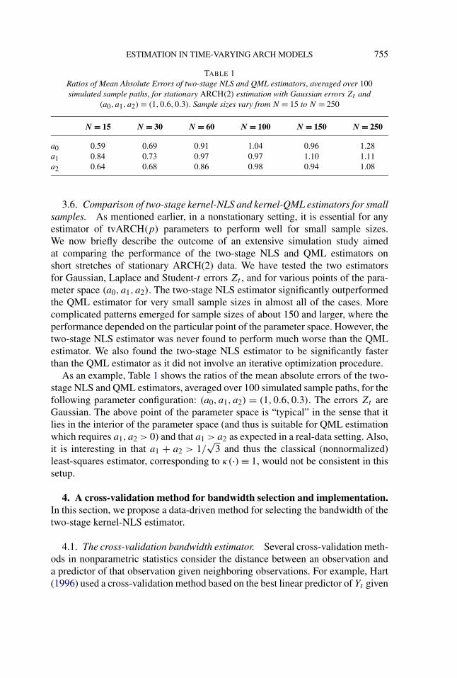
TABLE 1Ratios of Mean Absolute Errors of two-stage NLS and QML estimators, averaged over 100simulated sample paths, for stationary ARCH(2) estimation with Gaussian errors Zt and

(a0, a1, a2) = (1,0.6,0.3). Sample sizes vary from N = 15 to N = 250

N = 15 N = 30 N = 60 N = 100 N = 150 N = 250

a0 0.59 0.69 0.91 1.04 0.96 1.28a1 0.84 0.73 0.97 0.97 1.10 1.11a2 0.64 0.68 0.86 0.98 0.94 1.08

3.6. Comparison of two-stage kernel-NLS and kernel-QML estimators for smallsamples. As mentioned earlier, in a nonstationary setting, it is essential for anyestimator of tvARCH(p) parameters to perform well for small sample sizes.We now briefly describe the outcome of an extensive simulation study aimedat comparing the performance of the two-stage NLS and QML estimators onshort stretches of stationary ARCH(2) data. We have tested the two estimatorsfor Gaussian, Laplace and Student-t errors Zt , and for various points of the para-meter space (a0, a1, a2). The two-stage NLS estimator significantly outperformedthe QML estimator for very small sample sizes in almost all of the cases. Morecomplicated patterns emerged for sample sizes of about 150 and larger, where theperformance depended on the particular point of the parameter space. However, thetwo-stage NLS estimator was never found to perform much worse than the QMLestimator. We also found the two-stage NLS estimator to be significantly fasterthan the QML estimator as it did not involve an iterative optimization procedure.

As an example, Table 1 shows the ratios of the mean absolute errors of the two-stage NLS and QML estimators, averaged over 100 simulated sample paths, for thefollowing parameter configuration: (a0, a1, a2) = (1,0.6,0.3). The errors Zt areGaussian. The above point of the parameter space is “typical” in the sense that itlies in the interior of the parameter space (and thus is suitable for QML estimationwhich requires a1, a2 > 0) and that a1 > a2 as expected in a real-data setting. Also,it is interesting in that a1 + a2 > 1/

√3 and thus the classical (nonnormalized)

least-squares estimator, corresponding to κ(·) ≡ 1, would not be consistent in thissetup.

4. A cross-validation method for bandwidth selection and implementation.In this section, we propose a data-driven method for selecting the bandwidth of thetwo-stage kernel-NLS estimator.

4.1. The cross-validation bandwidth estimator. Several cross-validation meth-ods in nonparametric statistics consider the distance between an observation anda predictor of that observation given neighboring observations. For example, Hart(1996) used a cross-validation method based on the best linear predictor of Yt given


the past to select the bandwidth of a kernel smoother, where Yt was a nonparamet-ric function plus correlated noise. The methodology we propose is based on thebest linear predictor of X2

t,N given the past, which is a0(tN

)+∑pj=1 aj (

tN

)X2t−j,N .

We estimate the parameters {aj (t/N)}j using the localized two-stage kernel-NLS method but omit the observation X2

t,N in the estimation. More precisely, we

use a−tt,N (b) = (a−t

0 (b), . . . , a−tp (b)) as an estimator of {aj (t/N)}j , where

a−tt,N (b) = {R−t

t,N (b)}−1r−tt,N (b),(19)

with

R−tt,N (b) =

N∑k=p+1

k �=t,...,t+p

1

bNW

(t − k

bN

) Xk−1,NXTk−1,N

(μt,N + Sk−1,N )2 ,

r−tt,N (b) =

N∑k=p+1

k �=t,...,t+p

1

bNW

(t − k

bN

)X2

k,NXk−1,N

(μt,N + Sk−1,N )2 .

By using a−tt,N (b), the squared error in predicting X2

t,N is given by (X2t,N −

a−t0 (b) −∑p

j=1 a−tj (b)X2

t−j,N )2.To reduce the complexity, we suggest only evaluating the cross-validation cri-

terion on a subsample of the observations. Let h be such that h → ∞, N/h → ∞as N → ∞ (in practice h p). We implement the cross-validation criterion ononly the subsampled observations {Xkh,N :k = 1, . . . ,N/h}. In other words, leta

−khkh,N(b) = (a−kh

0 (b), . . . , a−khp (b)) be the estimator defined in (19) and by nor-

malizing the squared error with the term (μkh,N +∑pj=1 X2

kh−j,N)2, we define thefollowing cross-validation criterion

GN,h(b) = h

N

N/h∑k=1

(X2kh,N − a−kh

0 (b) −∑pj=1 a−kh

j (b)X2kh−j,N )2

(μkh,N +∑pj=1 X2

kh−j,N )2.(20)

We then use bhopt as the optimal bandwidth, where bh

opt = arg minbGN,h(b). Us-ing similar arguments to those in Hart (1996), asymptotically, one can show thatGN,h(b) is equivalent to the mean-squared error GN,h(b), where

GN,h(b) = h

N

N/h∑k=1

E

{(X2kh,N − a−kh

0 (b) −∑pj=1 a−kh

j (b)X2kh−j,N )2

(μkh,N +∑pj=1 X2

kh−j,N )2

}.(21)

It follows that bhopt is an estimator of bopt, where bopt = arg minb GN,h(b). GN,h(b)

is minimized if a−tkh,N(b) = a(kh/N) and in that case it is asymptotically equal to

∫ 1

0E

{(Z2

0 − 1)2σ 20 (u)

[μ(u) +∑pj=1 X2−j (u)]2

}du.(22)


FIG. 1. Dotted lines in the middle and right plots: the true time-varying parameters a0(u) anda1(u), respectively. The left plot: a sample path from the model, with Gaussian errors. Solid lines inthe middle and right plots: the corresponding estimates. See Section 4.2 for details.

Therefore, bhopt is such that a

−tt,N (bh

opt) is close to a(t/N).It is straightforward to show that the computational complexity of this algo-

rithm is O(B NhN log N), where B is the cardinality of the set of bandwidths tested

for the minimum of the cross-validation criterion. We note that the above rate isunattainable for the kernel-QML estimator due to its iterative character.

4.2. An illustrative example. We illustrate the performance of the proposedcross-validation criterion by an interesting example of a tvARCH(1) process forwhich the parameters a0(·) and a1(·) vary over time but the asymptotic uncondi-tional variance E(X2

t (u)) = a0(u)/(1 − a1(u)) remains constant. This means thatsample paths of {Xt,N }t will invariably appear stationary on visual inspection, andthat more sophisticated techniques are needed to detect the nonstationarity.

The left-hand plot in Figure 1 shows a sample path of length 1024, simulatedfrom the above process using standard Gaussian errors. The true time-varying pa-rameters a0(·) and a1(·) are displayed as dotted lines in the middle and right-handplots, respectively. In the estimation procedure, we used the Parzen kernel (a con-volution of the rectangular and triangular kernels) and, for simplicity, set μt,N tobe the sample mean of {X2

t,N }t . To estimate a suitable bandwidth, we applied theproposed cross-validation procedure described above with h = 10 (empirically, wehave found that for data of length of order 1000, the value h = 10 offers a goodcompromise between speed and accuracy of our method). We examined the valueof the cross-validation criterion over a regular grid of bandwidths between 0 and1, and obtained the optimal bandwidth as bh

opt = 0.132.The resulting parameter estimates are shown in the middle and right-hand plots

of Figure 1 as solid lines. While we can clearly observe a degree of bias due to thesmall sample sizes involved in the estimation, it is reassuring to see that the result-ing estimates correctly trace the shape of the underlying parameters. Denoting theempirical residuals from the fit by Zt , the p-value of the Kolmogorov–Smirnovtest for Gaussianity of Zt was 0.08, and the p-values of the Ljung–Box test forlack of serial correlation in Zt , |Zt | and Z2

t were 0.71, 0.33 and 0.58, respectively.


5. Constructing bootstrap pointwise confidence intervals. In parameter es-timation of linear time series, bootstrap methods are often used to obtain a good fi-nite sample approximation of the distribution of the parameter estimators. Schemesbased on estimating the residuals are often used [Franke and Kreiss (1992)]. In-spired by these methods, we propose a bootstrap scheme for the tvARCH(p)

process, which we use to construct pointwise confidence intervals for the two-stagekernel-NLS estimator. The main idea of the scheme is to use the two-stage kernel-NLS estimator to estimate the residuals. We construct the empirical distributionsfrom the estimated residuals, sample from it and use this to construct the bootstraptvARCH(p) sample. We show that the distribution of the two-stage kernel-NLSestimator using the bootstrap tvARCH(p) sample and the “true” tvARCH(p) esti-mator asymptotically coincide. We mention that the scheme and the asymptotic re-sults derived here are also of independent interest and can be used to bootstrap sta-tionary ARCH(p) processes [for a recent review on resampling and subsamplingfinancial time series in the stationary context, see Paparoditis and Politis (2007)].We emphasize that unlike the kernel-QML estimator, this computer-intensive pro-cedure is feasible for the kernel-NLS estimator due to its rapid computability.

Let at0,N= (at0,N (0), . . . , at0,N (p)). We first note that Assumption 1(i) is usu-

ally imposed in the tvARCH framework because it guarantees that almost surelyevery realization of the resulting process is bounded. When the sum of the coef-ficients is greater than one, the corresponding process is unstable. The followingresidual bootstrap scheme constructs the tvARCH(p) process from estimates of

the residuals and the parameter estimators. Despite at0,N

P→ a(u0), it is not neces-sarily true that the sum of the parameter estimates satisfies

∑pj=1 at0,N (j) < 1.

To overcome this, we now define a very slight modification of the two-stagekernel-NLS estimator which guarantees that this sum is less than one. Let at0,N

=(at0,N (0), . . . , at0,N (p)), where at0,N (0) = at0,N (0) and, for j > 1,

at0,N (j) =

⎧⎪⎪⎪⎪⎪⎨⎪⎪⎪⎪⎪⎩

at0,N (j), ifp∑

j=1

at0,N (j) ≤ 1 − δ,

(1 − δ)at0,N (j)∑p

j=1 at0,N (j), if

p∑j=1

at0,N (j) > 1 − δ.

(23)

Since at0,N

P→ a(u0) and∑p

j=1 aj (u) ≤ 1 − δ [Assumption 1(i)], it is straightfor-

ward to see that at0,N

P→ a(u0) and∑p

j=1 at0,N (j) ≤ 1 − δ.The residual bootstrap of the tvARCH (p) process:

(i) If k ∈ [t0 − bN, t0 + bN − 1], using the parameter estimators constructresiduals

Z2k = X2

k,N

at0,N (0) +∑pj=1 at0,N (j)X2

k−j,N

.


(ii) Define Z2t = Z2

t − 12bN

∑t0+bN−1k=t0−bN Z2

k + 1 and consider the empirical dis-tribution function

Ft0,N (x) = 1

bN

t0+bN−1∑k=t0−bN

I(−∞,x](Z2k ),

where IA(y) = 1 if y ∈ A, 0 otherwise. It is worth mentioning that we use Z2t

rather than Z2t since we have E(Z2

t ) = ∫zFt0,N (dz) = 1. (This result is used in

Proposition 6 in the Appendix.)Set X+2

t (u0) = 0 for t ≤ 0. For 1 ≤ t ≤ t0 + bN/2, sample from the distributionfunction Ft0,N (x), to obtain the sample {Z+2

t }t . Use this to construct the bootstrapsample

X+2t (u0) = σ+2

t (u0)Z+2t , σ+2

t (u0) = at0,N (0) +p∑

j=1

at0,N (j)X+2t−j (u0).

We note that by estimating the residuals from [t0 − bN, t0 + bN − 1], the distri-bution of X+2

t (u0) will be suitably close to the stationary approximation Xt(u0)

when t ∈ [t0 − bN/2, t0 + bN/2 − 1], this allows us to obtain the sampling prop-erties of the bootstrap estimator.

(iii) Define the bootstrap estimator

a+t0,N

= {R+t0,N

}−1r+t0,N

,(24)

where Xt−1(u0)+ = (1,X+2

t−1(u0), . . . ,X+2t−p(u0))

T and

R+t0,N

=N∑

k=p+1

1

bNW

(t0 − k

bN

)Xk−1(u0)

+Xk−1(u0)+T

(μt0,N +∑kj=1 X+2

k−j (u0))2,

r+t0,N

=N∑

k=p+1

1

bNW

(t0 − k

bN

)X+2

k (u0)Xk−1(u0)+T

(μt0,N +∑kj=1 X+2

k−j (u0))2.

We observe that in steps (i), (ii) of the bootstrap scheme we are constructing thebootstrap sample {X+2

t (u0)}t whose distribution should emulate the distribution ofthe stationary approximation {X2

t (u0)}t . In step (iii) of the bootstrap scheme weare constructing the bootstrap estimator a

+t0,N

from the bootstrap samples. We note

that we have bootstrapped the stationary approximation X2t (u0) since the limiting

distribution of at0,Nis derived using the stationary approximation.

We now show that the distributions of√

bN{a+t0,N

− at0,N} and

√bN{at0,N

−a(u0)} asymptotically coincide.

PROPOSITION 5. Suppose Assumption 1 holds, and suppose eitherinfj aj (u0) > 0 or E(Z4

t )1/2 supu[

∑pj=1 aj (u)] < 1 − δ [which implies


supk E(X4k,N) < ∞]. Let at0,N

and a+t0,N

be defined as in (23) and (24), respec-

tively, and let bβ√

bN → 0. If |u0 − t0/N | < 1/N , then we have√

bN(a+t0,N

− at0,N)

D→ N(0,w2μ4

{E[A

(μ)t (u0)

]}−1{E[D

(μ)t (u0)

]}{E[A

(μ)t (u0)

]}−1),

with b → 0, bN → ∞ as N → ∞.

Comparing the results in Propositions 4(ii) and Propositions 5 we see ifbβ

√bN → 0, then, asymptotically, the distributions of (a

+t0,N

− at0,N) and (at0,N

−a(u0)) are the same.

6. Volatility estimation: real data examples. The datasets analyzed in thisand the following section fall into two categories:

1. Logged and differenced daily exchange rates between USD and a number ofother currencies running from January 1, 1990 to December 31, 1999: thedata are available from the US Federal Reserve website: www.federalreserve.gov/releases/h10/Hist/default1999.htm. We use the following acronyms: CHF(Switzerland Franc), GBP (United Kingdom Pound), HKD (Hong Kong Dol-lar), JPY (Japan Yen), NOK (Norway Kroner), NZD (New Zealand Dollar),SEK (Sweden Kronor), TWD (Taiwan New Dollar).

2. Logged and differenced daily closing values of the NIKKEI, FTSE, S andP500 and DAX indices, measured between a date in 1996 (exact dates vary)and April 29, 2005: the data are available from: www.bossa.pl/notowania/daneatech/metastock/.

The lengths N of each dataset vary but oscillate around 2500. In this section, weexhibit the estimation performance of the two-stage kernel-NLS estimator on theUSD/GBP exchange rate and FTSE series. We examine the cases p = 0,1,2 anduse the Parzen kernel with bandwidths selected by the cross-validation algorithmof Section 4.2.

The left column in Figure 2 shows the results for USD/GBP. The top plot showsthe data, the next one down shows the estimates of a0(·) for p = 0 (dashed line),p = 1 (dotted line) and p = 2 (solid line), the one below displays the positive partsof the estimates of a1(·) for p = 1 (dotted) and p = 2 (solid), and the bottom plotshows the positive part of the estimate of a2(·) for p = 2. Note that the negativevalues arise since our estimator is not guaranteed to be nonnegative. The rightcolumn shows the corresponding quantities for the FTSE data. It is interesting toobserve that in both cases, the shapes of the estimated time-varying parameters aresimilar for different values of p.

The goodness of fit for each choice of p = 0,1,2 is assessed in Table 2. In eachcase, Zt denotes the sequence of empirical residuals from the given fit. For the

www.federalreserve.gov/releases/h10/Hist/default1999.htm

www.bossa.pl/notowania/daneatech/metastock/

www.federalreserve.gov/releases/h10/Hist/default1999.htm

www.bossa.pl/notowania/daneatech/metastock/


FIG. 2. Left (right) column: USD/GBP (FTSE) series and the corresponding estimation results. SeeSection 6 for details.

USD/GBP data, the best fit is obtained for p = 1. For the FTSE data, it is lessclear which order gives the best fit but the Ljung–Box (L–B) p-value for |Zt | isthe highest for p = 0 and thus it seems to be the preferred option, which is furtherconfirmed by the visual inspection of the sample autocorrelation function of |Zt |in the three cases. In both cases, the empirical residuals are negatively skewed, andin the case of USD/GBP they are also heavy-tailed.


TABLE 2The values of bandwidth selected by cross-validation, the p-values of the L–B test for white noisefor Zt , |Zt |, Z2

t , and the sample skewness and kurtosis coefficients for Zt for the USD/GBP andFTSE data sets. The boxed value means p-value is below 0.05

USD/GBP FTSE

p = 0 p = 1 p = 2 p = 0 p = 1 p = 2

Bandwidth 0.02 0.032 0.04 0.024 0.028 0.028L–B P -value for Zt 0.83 0.83 0.82 0.15 0.20 0.30

L–B P -value for |Zt | 0.17 0.71 0.03 0.10 0.07 0.07L–B P -value for Z2

t 0.09 0.79 0.26 0.13 0.35 0.52Skewness of Zt −0.05 −0.09 −0.08 −0.13 −0.15 −0.16Kurtosis of Zt 0.7 0.92 1.24 −0.01 0.06 0.15

We conclude this section by constructing bootstrap pointwise confidence inter-vals for the estimated parameters, using the algorithm detailed in Section 5. Notethat our central limit theorem (CLT) of Proposition 4 could be used for the samepurpose, but this would require pre-estimation of a number of quantities, whichwe wanted to avoid. We base our bootstrap pointwise confidence intervals on 100bootstrap samples. For clarity, we only display confidence intervals for the “pre-ferred” orders p: that is, for p = 1 in the case of the USD/GBP data, and p = 0 inthe case of the FTSE series. These are shown in Figure 3.

It is interesting to note that the pointwise confidence intervals for the “nonlin-earity” parameter a1(·) in the USD/GBP series are relatively wide and that theparameter can be viewed as only insignificantly different from zero most (but notall) of the time. On the other hand, there exist time intervals where the parametersignificantly deviates from zero. This further confirms the observation made ear-lier that the order p = 0 is an inferior modeling choice for this series and that theorder p = 1 is preferred.

7. Volatility forecasting: real data examples. In this section, we describea numerical study whereby the long-term volatility forecasting ability of thetvARCH(p) process is compared to that of the stationary GARCH(1,1) andEGARCH(1, 1) processes with standard Gaussian errors. We compute the fore-casts of the tvARCH(p) process as follows: we use the available data to estimatethe tvARCH(p) parameters, and then forecast into the future using the “last” es-timated parameter values, that is, those corresponding to the right edge of the ob-served data. For a rectangular kernel with span m, this strategy leads to the fol-lowing algorithm: (a) treat the last m data points as if they came from a stationaryARCH(p) process, (b) estimate the stationary ARCH(p) parameters on this seg-ment (via the two-stage NLS scheme), and (c) forecast into the future as in the


FIG. 3. Solid lines from left to right: estimates of a0(·) for USD/GBP, a1(·) for USD/GBP, and a0(·)for FTSE. Dashed lines: the corresponding 80% symmetric bootstrap pointwise confidence intervals.

classical stationary ARCH(p) forecasting theory [for the latter, see, e.g., Bera andHiggins (1993)].

We denote the mean-square-optimal h-step-ahead volatility forecasts at time t ,obtained via the above algorithm, by σ

2,tvARCH(p)t |t+h . Note that to obtain the analo-

gous quantities, σ 2,GARCH(1,1)t |t+h and σ

2,EGARCH(1,1)t |t+h , for the stationary GARCH(1,1)

and EGARCH(1, 1) processes, we always use the entire available dataset, and notonly the last m observations.

To test the forecasting ability of the various models, we use the exchange rateand stock index datasets listed in Section 6. For the tvARCH(p) process, we takep = 0,1,2, and use the forecasting procedure described above with a rectangularkernel, over a grid of span values m = 50,100, . . . ,500. Note that the tvARCH(0)process has the simple form Xt,N = a

1/20 (t/N)Zt and is also considered by Starica

and Granger (2005). We select the span by a “forward validation” procedure, thatis, choose the value of m that yields the minimum out-of-sample prediction errorAMSE defined below.

For the stationary (E)GARCH(1,1) prediction, we use the standard S-Plusgarch and predict routines. The stationary (E)GARCH(1,1) parameters arere-estimated for each t .

For each t = 1000, . . . ,N − 250, we compute the quantities

σ2,modelt |t+250 =

250∑h=1

σ2,modelt |t+h ,

where “model” is one of: tvARCH(0), tvARCH(1), tvARCH(2), GARCH(1,1),and EGARCH(1,1), and compare them to the “realized” volatility

X2t |t+250 =

250∑h=1

X2t+h,


using the scaled aggregated mean square error (AMSE)

Rmodel250,1000,N =

N−250∑t=1000

(σ2,modelt |t+250 − X

2t |t+250)

2,

where the scaling is by the factor of 1/(N − 1000). For a justification of thissimulation setup, see Starica (2003).

Table 3 lists the AMSEs attained by tvARCH(0), tvARCH(1), tvARCH(2), sta-tionary GARCH(1,1) and stationary EGARCH(1, 1) processes: the best resultsare boxed. The values in brackets indicate the selected span values. The bulletsfor the USD/TWD and USD/HKD series indicate that the numerical optimizersperforming the QML estimation in stationary (E)GARCH(1,1) processes failed toconverge at several points of the series and, therefore, we were unable to obtainaccurate forecasts. We list below some interesting conclusions from this study.

• In most cases, the selected span values m are similar across orders p. Thesevalues can be taken as an indication of how “variable” the time-varying parame-ters are. Exceptions to this rule occur mostly in data sets which are difficult tomodel, such as the HKD series, which is extremely spiky. For the latter series,more thought is needed on how to model it accurately in the tvARCH(p) (orindeed any other) framework.

• For the NZD series, it can clearly be seen how “adding more nonlinearity takesaway nonstationarity”: as p increases, a larger and larger span m is selected,which means that more and more variability in the volatility of the data can beattributed to the nonlinearity, rather than the nonstationarity.

• While the tvARCH(p) framework seems superior to stationary (E)GARCH(1,1)

methodology for the currency exchange data, the opposite is true for the stockindices. This might be indicative of the fact that stock indices are “less nonsta-tionary” than currency exchange series.

We conclude with a heuristic investigation of the quality of our volatility fore-casts. Conditioning on the information available up to time t , the quantity σ

2,modelt |t+250

predicts the variance of the variable X(250)t := ∑250

h=1 Xt+h. By CLT-type argu-

ments, X(250)t is approximately Gaussian, and thus we assess the quality of the

predicted volatility by measuring how often the process Yt := X(250)t /{σ 2,model

t |t+250}1/2

falls into desired confidence intervals for standard Gaussian variables.However, this is less informative of the quality of the forecasting procedure

than one might hope, the reason being that the process Yt is strongly dependent,so it is not reasonable to expect it to take values outside (1 − α)100% confidenceintervals exactly, or approximately, 100α% of the time. Figure 4 shows processesYt constructed for the GBP, NZD and SEK series, with the “optimal” forecastingparameters from Table 3 (i.e., those for which the results are boxed). For α = 0.05,the coverages are, respectively, 100%, 79% and 95%. If the dependence in Yt were


TABLE 3AMSE for long-term forecasts using tvARCH (0), tvARCH (1), tvARCH (2), stationary

GARCH (1,1) and stationary EGARCH(1, 1) processes. R(E)GARCH(1,1)250,1000,N is the better result out of:

RGARCH(1,1)250,1000,N and R

EGARCH(1,1)250,1000,N

Series Scaling R(E)GARCH(1,1)250,1000,N R

tvARCH(0)250,1000,N R

tvARCH(1)250,1000,N R

tvARCH(2)250,1000,N

CHF 108 2395 2371 (500) 2254 (500) 3030 (500)

GBP 109 20282 7660 (250) 9567 (300) 9230 (300)

HKD 1012 • 230 (150) 170 (500) 150 (100)

JPY 108 8687 9713 (350) 9173 (300) 9450 (300)

NOK 108 1767 1552 (500) 1875 (250) 2221 (500)

NZD 108 11890 5270 (50) 4976 (100) 4955 (150)

SEK 109 37720 6639 (250) 6805 (250) 7321 (250)

TWD 108 • 2323 (500) 2372 (500) 2400 (500)

S & P500 105 33 43 (500) 43 (500) 40 (500)

FTSE 106 516 860 (500) 958 (500) 983 (500)

DAX 106 2602 4492 (150) 4483 (500) 4864 (150)

NIKKEI 107 2364 3418 (100) 3252 (250) 3432 (250)

weaker, we would expect the three coverages to be closer to 95%, provided theforecasting procedure was “adequate.” However, here, the strong dependence in Yt

causes the variance of the coverage percentages to be high.Nonetheless, it is reassuring to note that on average, across the datasets, we

do obtain the correct coverage of around 95%. To see this, let us consider theseries for which our forecasting procedure is satisfactory [i.e., those for whichit outperforms (E)GARCH(1,1) processes], bar the two series: HKD and TWD,which are extremely spiky and thus difficult to model and forecast. These are:CHF, GBP, NOK, NZD, SEK. Table 4 shows the coverages for the five series.The average coverage is 94.2%, which is very close to the ideal coverage of 95%.Averaging across all series, excluding HKD and TWD, we obtain a coverage of95.7%.

TABLE 4Coverage of 95% Gaussian prediction intervals for our method, using parameter configurations

that gave the best results in Table 3

Series CHF GBP NOK NZD SEK

Coverage 99% 100% 98% 79% 95%


FIG. 4. From top to bottom: processes Yt for the GBP, NZD, SEK series. Horizontal lines: symmet-ric 95% confidence intervals for standard Gaussian variables.

APPENDIX: AUXILIARY LEMMAS AND OUTLINE OF PROOFS

The aim of this Appendix is to sketch the proofs of the results stated in theprevious sections. The full details can be found in a technical report, availablefrom the authors or from http://www.maths.bris.ac.uk/~mapzf/tvarch/trNLS.pdf.

http://www.maths.bris.ac.uk/~mapzf/tvarch/trNLS.pdf


Before proving these results, we first obtain some results related to weightedsums of tvARCH(p) processes that we use below.

In what follows, we use K to denote a generic finite positive constant.

A.1. Properties of tvARCH(p) processes. Let us define the following quan-tity:

r(u) = E

{X2

k(u)Xk−1(u)

κ(u0,Xk−1,N )2

}.(25)

LEMMA A.1. Suppose the conditions in Proposition 3(i) are satisfied, letμ(u) = E{X2

t (u)}, and let At (u), Dt (u) and r(u) be defined as in (8) and (25),respectively. If |u0 − t0/N | < 1/N , then we have:

(i)

N∑k=1

1

bNW

(t0 − k

bN

)X2

k,N

P→ μ(u0).(26)

(ii)

Rt0,N=

N∑k=p+1

1

bNW

(t0 − k

bN

)Xk−1,NXTk−1,N

κ(u0,Xk−1,N )2P→ E[At (u0)].(27)

(iii)

rt0,N=

N∑k=p+1

1

bNW

(t0 − k

bN

)X2

k,NXk−1,N

κ(u0,Xk−1,N )2P→ r(u0).(28)

(iv) Suppose further that the conditions in Proposition 3(ii) are satisfied, thenwe have

N∑k=p+1

1

bNW 2(

t0 − k

bN

)σ 4

k,NXk−1,NXTk−1,N

κ(u0,Xk−1,N )4P→ w2E[Dt (u0)],(29)

with b → 0, bN → ∞ as N → ∞, where w2 = ∫ 1/2−1/2 W 2(x)dx.

PROOF. It is straightforward to derive (i), (ii), (iii) and (iv) using Lemma A.5in Dahlhaus and Subba Rao (2006). We omit the details. �

To prove Lemma A.3 below we use the following lemma, whose proof is basedon mixingale arguments. Suppose 1 ≤ q < ∞, and let ‖ · ‖q denote the �q -norm ofa vector.


LEMMA A.2. Suppose {φk : k = 1,2, . . .} is a stochastic process whichsatisfies E(φk) = 0 and E(φ

qk ) < ∞ for some 1 < q ≤ 2. Further, let Ft =

σ(φt , φt−1, . . .), and suppose that there exists a ρ ∈ (0,1) such that {E‖E(φk|Fk−j )‖q

q}1/q ≤ Kρj . Then we have

{E

∥∥∥∥∥s∑

k=1

akφk

∥∥∥∥∥q

q

}1/q

≤ K

1 − ρ

(s∑

k=1

|ak|q)1/q

.(30)

In Lemma A.3 below we derive rates of convergence for local sums of a sta-tionary ARCH(p) process. We use this result to prove the long memory result inProposition 2.

Let us define the following quantities:

μ1(u, d,h) = E{X2t (u)X2

t+h(u + d)},(31)

c(u, d,h) = cov{X2t (u), X2

t+h(u + d)},and set μ1(u,0, h) = μ1(u,h) and c(u,0, h) = c(u,h). Define also the followingquantities:

Sk,bN(u) = 1

bN

(k+1)bN−1∑s=kbN

X2s (u),(32)

Sk,bN(u,h, d) = 1

bN

(k+1)bN−1∑s=kbN

X2s (u)X2

s+h(u + d).(33)

LEMMA A.3. Suppose {Xt (u)}t is a stationary ARCH(p) process defined asin (2) and suppose the conditions on the parameters {aj (u)}j and the innovations{Zt } in Assumption 1(i), (ii), (iv) hold. Let μ(u) = E{X2

t (u)}, and let μ1(u, d,h),Sk,bN(u) and Sk,bN(u,h, d) be defined as in (31), (32) and (33) respectively. Then,we have {

E

∥∥∥∥∥N∑

k=p+1

1

bNW

(t − k

bN

){X2

k(u) − μ(u)}∥∥∥∥∥

1+η

1+η

}1/(1+η)

(34)≤ K(bN)−(η)/1+η.

Further, if {E(|Zt |2(2+ζ ))}1/(2+ζ ) supu

∑pj=1 aj (u) ≤ 1 − δ for some 0 < ζ ≤ 2

and δ > 0, then we have

{E‖Sk,bN(u,h, d) − μ1(u, d,h)‖1+ζ/21+ζ/2}1/(1+ζ/2) ≤ K(bN)−(ζ )/2+ζ ,(35)

where the constant K is independent of u and d .


PROOF. We will first prove (34). We use Lemma A.2, with ak = W(t−kbN

),φk = {X2

k(u) − μ(u)} and q = 1 + η. It can be shown that

{‖E(X2k(u) | Fk−j ) − μ(u)‖1+η

1+η}1/(1+η)

≤ Kρj (1 + {E‖Xk−j (u)‖1+η1+η}1/(1+η)),

where Ft = σ(X2t (u), X2

t−1(u), . . .). By using the above and that the support ofW(t−k

bN) is proportional to bN , we can apply Lemma A.2 to obtain

{E

∥∥∥∥∥N∑

k=p+1

1

bNW

(t − k

bN

){X2

k(u) − μ(u)}∥∥∥∥∥

1+η

1+η

}1/(1+η)

≤ 1

bN

K

1 − ρ

(N∑

k=p+1

∣∣∣∣W(

t − k

bN

)∣∣∣∣1+η

)1/(1+η)

≤ K(bN)−η/(1+η).

Thus, we have proved (34). The proof of (35) is similar to the proof above butrequires the additional (stated) assumption, hence we omit the details. �

A.2. The covariance structure and the long memory effect of tvARCH(p)processes. In this section, we prove results for the covariance structure and thelong memory effect of tvARCH(p) processes.

PROOF OF PROPOSITION 1. It follows easily by making a time-varyingVolterra series expansion of the tvARCH(p) process [see Section 5 in Dahlhausand Subba Rao (2006)] and using Lemma 2.1 in Giraitis, Kokoszka and Leipus(2000). We omit the details. �

The following lemma is used to prove Proposition 2.

LEMMA A.4. Suppose {Xt,N }t is a tvARCH(p) which satisfies Assumption1(i), (ii), (iv), and let {Xt (u)}t be defined as in (2). Let h := h(N) be such thath/N → d ∈ [0,1) as N → ∞. Then we have

1

N − h

N−h∑s=1

X2s,N

P→∫ 1−d

0E{X2

t (u)}du.(36)

Further, if {E(|Zt |2(2+ζ ))}1/(2+ζ ) supu

∑pj=1 aj (u) ≤ 1 − δ for some 0 < ζ ≤ 2

and δ > 0, then we have

1

N − h

N−h∑s=1

X2s,NX2

s+h,N

P→∫ 1−d

0E{X2

t (u)X2t+h(u + d)}du.(37)


PROOF. We first prove (37). Let b := b(N) be such that 1/b is an inte-ger, b → 0 and b(N − h) → ∞ as N → ∞. We partition the left-hand side of(37) into 1/b blocks. Let kb = kb[1 − d], and replace the terms X2

kb(N−h)+r,N

and X2kb(N−h)+r+h,N with X2

kb(N−h)+r (kb) and X2kb(N−h)+r+h(kb + d), respec-

tively. Let N ′ = (N − h). If s ∈ [kbN ′, (k + 1)bN ′) then we replace X2s,N with

X2s (kb) and X2

s+h,N with X2s (kb + d). Recall the notation Sk,bN(u,h, d) and

μ1(u, d,h) given in (31) and (33), respectively. Now, by using Lemma 1 and thatkb(N−h)

N≤ s

N< (k+1)b(N−h)

N, we have

1

N − h

N−h∑s=1

X2s,NX2

s+h,N

(38)

= b

1/b−1∑k=0

1

b(N − h)

b(N−h)−1∑r=0

Sk,bN(kb, h, d) + RN,

where

|RN | ≤ b

1/b−1∑k=0

1

bN ′bN ′−1∑r=0

{X2

kbN ′+r,N

(1

NβVkbN ′+r+h,N

+(

2b +∣∣∣∣ hN − d

∣∣∣∣)β

WkbN ′+r+h

)

+ X2kbN ′+r+h(kb + d)

(1

NβVkbN ′+r,N

+ (2b)βWkbN ′+r

)}.

Now, taking expectations of the above, we have

(E|RN |1+ζ/2)1/(1+ζ/2) ≤ K

{(2b + b

∣∣∣∣d − h

N

∣∣∣∣)β

+ 1

Nβ

}.(39)

Therefore, RNP→ 0 as N → ∞. By substituting the integral

∫ 1−d0 μ1(u, d,h) du

with a sum and using (38) and (39), we have{E

∥∥∥∥∥ 1

N − h

N−h∑s=1

X2s,NX2

s+h,N −∫ 1−d

0μ1(u, d,h) du

∥∥∥∥∥1+ζ/2

1+ζ/2

}1/(1+ζ/2)

≤ b

1/b−1∑k=0

{E‖Sk,b(N−h)(kb, h, d) − μ1(kb, d,h)‖1+ζ/21+ζ/2}1/(1+ζ/2)

(40)

+∣∣∣∣∣b

1/b−1∑k=0

μ1(kb, d,h) −∫ 1−d

0μ1(kb, d,h) du

∣∣∣∣∣


+ O

{(b + kb

∣∣∣∣d − h

N

∣∣∣∣)β

+ 1

Nβ

}.

Finally, by substituting the bound (35) and∣∣∣∣∣b1/b−1∑k=0

μ1(kb, d,h) −∫ 1−d

0E{X2

t (u)X2t+h(u + d)}du

∣∣∣∣∣≤ kb

into (40), we have{E

∥∥∥∥∥ 1

N − h

N−h∑s=1

X2s,NX2

s+h,N

−∫ 1−d

0E{X2

t (u)X2t+h(u + d)}du

∥∥∥∥∥1+ζ/2

1+ζ/2

}1/(1+ζ/2)

→ 0,

which gives us (37). The proof of (36) is similar and we omit the details. �

PROOF OF PROPOSITION 2. We first consider the more general case whereh := h(N) is such that h/N → d ∈ [0,1) as N → ∞. Then, for fixed h > 0, weobtain (5) as special case with d = 0.

Let SN(h) = AN − BN , where

AN = 1

N − h

N−h∑t=1

X2t,NX2

t+h,N and BN = (XN)2.

We consider the asymptotic behavior of the terms AN and BN separately. By using(36) and (37), we have

ANP→∫ 1−d

0μ1(u,h, d) du and BN

P→∫ 1−d

0

∫ 1−d

0μ(u)μ(v) dudv.

Recall that μ(u) = E{X2t (u)}, and that μ1(u, d,h) and c(u, d,h) are defined in

(31). By using the formula μ1(u, d,h) = c(u, d,h) + μ(u)μ(u + d), we obtain

SN(h)P→∫ 1−d

0{c(u, d,h) + μ(u)μ(u + d)}du −

{∫ 1−d

0μ(u)du

}2

(41)

where h/N → d as N → ∞.Let us now consider the special case of (41) where d = 0. Then, for fixed h > 0,

we have

SN(h)P→∫ 1

0c(u,h) du +

∫ 1

0

∫ 1

0μ2(u) dudv −

∫ 1

0

∫ 1

0μ(u)μ(v) dudv,

as N → ∞. This proves (5) and, hence, we have the required result. �


A.3. Proofs in Section 3.2. In this section, we prove consistency and asymp-totic normality of the weighted kernel-NLS estimator.

PROOF OF PROPOSITION 3(I). By using (27), (28) and Slutsky’s theorem, wehave

at0,N= {Rt0,N

}−1rt0,N

P→ {E[At (u0)]}−1r (u0).

Therefore, to prove that at0,N

P→ a(u0), we need to show that a(u0) ={E[At (u0)]}−1r (u0). By using (2) and dividing by κ(u0, Xk−1(u0)), {X2

k−1(u0)}ksatisfies the representation

X2k(u0)

κ(u0, Xk−1(u0))= aT (u0)Xk−1(u0)

κ(u0, Xk−1(u0))+ (Z2

k − 1)σ 2

k (u0)

κ(u0, Xk−1(u0)).(42)

Finally, multiplying (42) by Xk−1(u0)/κ(u0,Xk−1,N ) and taking on both sidesexpectations, we obtain the desired result.

To prove Proposition 3(ii), we use the same methodology given in the proof ofTheorem 3 in Dahlhaus and Subba Rao (2006), hence we omit the details. �

A.4. Proofs in Section 3.4. In this section, we prove consistency and asymp-totic normality of the two-stage kernel-NLS estimator. To prove these asymptoticproperties, we need the following two lemmas.

LEMMA A.5. Suppose {Xt,N }t is a tvARCH(p) process which satisfies As-sumption 1(i), (ii), (iv), let μ(u) = E{X2

t (u)}, and let μt0,N be defined as in (15).If |u0 − t0/N | < 1/N , then, for 0 ≤ i, j ≤ p, we have

N∑k=p+1

1

bNW

(t0 − k

bN

) X2k−i,NX2

k−j,N

(μt0,N + Sk−1,N )2P→ E

( X2k−i(u0)X

2k−j (u0)

(μ(u0) + Sk−1(u0))2

),(43)

with b → 0, bN → ∞ as N → ∞.

PROOF. To prove the result we use techniques similar to those in Bose andMukherjee (2003). By using the inequality |1/x2 − 1/y2| ≤ 2|x − y|{(1/x)[1 +x/y]}3, for x, y > 0, we bound the difference∣∣∣∣ X2

k−i,NX2k−j,N

(μt0,N + Sk−1,N )2 − X2k−i,NX2

k−j,N

(μ(u0) + Sk−1,N )2

∣∣∣∣≤ 2X2

k−i,NX2k−j,N |μt0,N − μ(u0)|

(44)

×∣∣∣∣ 1

μ(u0) + Sk−1,N

(1 + μt0,N + Sk−1,N

μ(u0) + Sk−1,N

)∣∣∣∣3

≤ 2|μt0,N − μ(u0)|(

1 + |μ(u0)||μt0,N |

) X2k−i,NX2

k−j,N

(μ(u0) + Sk−1,N )3 .


Let us now define the following quantities:

�(u0) = E

( X2k−i(u0)X

2k−j (u0)

{μ(u0) + Sk−1(u0)}2

),

At0,N =N∑

k=p+1

1

bNW

(t0 − k

bN

) X2k−i,NX2

k−j,N

{μt0,N + Sk−1,N }2 ,

Ct0,N (u0) =∣∣∣∣∣

N∑k=p+1

1

bNW

(t0 − k

bN

) X2k−i,NX2

k−j,N

{μ(u0) + Sk−1,N }2 − �(u0)

∣∣∣∣∣.Then, by using the bound (44), we have∣∣∣∣At0,N − �(u0)

∣∣∣∣∣≤∣∣∣∣

N∑k=p+1

1

bNW

(t0 − k

bN

) X2k−i,NX2

k−j,N

{μ(u0) + Sk−1,N }2 − �(u0)

∣∣∣∣∣+ 2|μt0,N − μ(u0)|

(1 + |μ(u0)|

|μt0,N |)

(45)

×N∑

k=p+1

1

bN

∣∣∣∣W(

t0 − k

bN

)∣∣∣∣ X2k−i,NX2

k−j,N

{μ(u0) + Sk−1,N }3

≤ Ct0,N (u0) + 2|μt0,N − μ(u0)|(

1 + |μ(u0)||μt0,N |

) N∑k=p+1

1

bN

∣∣∣∣W(

t0 − k

bN

)∣∣∣∣.Since μt0,N

P→ μ(u0), by using Slutsky’s lemma we have

|μt0,N − μ(u0)|(

1 + |μ(u0)||μt0,N |

)P→ 0.

Furthermore, by using (27) we have Ct0,N (u0)P→ 0. Altogether this gives |At0,N −

�(u0)| P→ 0, and the desired result follows. �

To show asymptotic normality, we need to define the following least-squarescriteria:

Lt0,N(α) =

N∑k=p+1

1

bNW

(t0 − k

bN

)ht0,N (Xk,N ,Xk−1,N ,α),(46)

Lt0(u,α) =

N∑k=p+1

1

bNW

(t0 − k

bN

)ht0,N (Xk(u), Xk−1(u),α),(47)


L(μ)t0

(u,α) =N∑

k=p+1

1

bNW

(t0 − k

bN

)h(u, Xk(u), Xk−1(u),α),(48)

where ht0,N(y0, y,α) = (μt0,N +∑p

j=1 y2j )−2{y2

p −α0−∑pj=1 αjy

2j }2 and h(u, y0,

y,α) = (μ(u) + ∑pj=1 y2

j )−2{y20 − α0 − ∑p

j=1 αjy2j }2. We note that at0,N

=arg mina Lt0,N

(a). Asymptotic normality of√

bN∇L(μ)t0

(u0, a(u0)) can easilybe established by verifying the conditions of the martingale central limit theo-rem. However, the same theorem cannot be used to show the asymptotic nor-mality of

√bN∇Lt0(u0, a(u0)), since Lt0(u0, a(u0)) is not a sum of martin-

gale differences. In Lemma A.6 below we overcome this problem by showing

that√

bN(Lt0(u0, a(u0)) − L(μ)t0

(u0, a(u0)))P→ 0, which allows us to replace

Lt0(u0, a(u0)) with L(μ)t0

(u0, a(u0)).

LEMMA A.6. Suppose {Xt,N }t is a tvARCH(p) process which satisfies As-sumption 1(i), (ii), (iii), (iv). Let μ(u) = E{X2

t (u)}, and μt0,N , Lt0(u,α) and

L(μ)t0

(u,α) be defined as in (15), (47) and (48), respectively. If |u0 − t0| < 1/N ,then we have

|μt0,N − μ(u0)| = Op

(bβ + (bN)−η/(1+η)),(49)

and √bN[∇Lt0(u0, a(u0)) − ∇L

(μ)t0

(u0, a(u0))]= op(1),(50)

with b → 0, bN → ∞ as N → ∞.

PROOF OF PROPOSITION 4. (i) It is straightforward to show consistency using(17) and Lemma A.5.

(ii) Define Bt0,N(α) = Lt0,N

(α) − Lt0(u,α). To prove that ∇Bt0,N (a(u0)) =

Op(bβ), we use the same arguments given in Theorem 3 in Dahlhaus and SubbaRao (2006), hence we omit the details. To prove (17), we use that ∇Lt0,N (at0,N

) =0, and expanding ∇Lt0,N (at0,N

) about a(u0), we have

∇2Lt0,N

(at0,N

− a(u0))

= L(μ)t0

(u0, a(u0)) + {∇Lt0(u0, a(u0)) − ∇L(μ)t0

(u0, a(u0))}

− ∇Bt0,N (a(u0)).

By using Lemma A.5, we easily see that ∇2Lt0,N (a(u0))P→ 2E[A(μ)

t (u0)] and,using (50), we have(

at0,N− a(u0)

)= −1

2

{∇L(μ)t0

(u0, a(u0)) + ∇Bt0,N (a(u0))}{

E[A

(μ)t (u0)

]}−1 + op

(1

bN

).


Finally, by using the martingale central limit theorem [see, e.g., Hall and Heyde(1980), Theorem 3.2], we obtain (17). �

A.5. Proofs in Section 5. In this section, we prove the results in Section 5.Some of the results in this section have been inspired by corresponding results inthe residual bootstrap for linear processes literature [cf. Franke and Kreiss (1992)].However, the proofs are technically very different, because the tvARCH(p)

process is a nonlinear, nonstationary process, and the normalization of the two-stage kernel-NLS estimator with random weights.

In order to show that the distribution of the bootstrap sample a+t0,N

− at0,Nas-

ymptotically coincides with the asymptotic distribution of at0,N− a(u0), we will

show convergence of the distributions under the Mallows distance. The Mallowsdistance between the distribution H and G is defined as

d2(H,G) = infX∼H,Y∼G

{E(X − Y)2}1/2.

Roughly speaking, if d2(Fn,Gn) → 0, then the limiting distributions of Fn and Gn

are the same [Bickel and Freedman (1981)]. Following Franke and Kreiss (1992),to reduce notation, we let d2(X,Y ) = d2(H,G), where the random variables X

and Y have measures H and G, respectively.We also require the following definitions. Let

RN(u0) =N∑

k=p+1

1

bNW

(t0 − k

bN

)Xk−1(u0)Xk−1(u0)

T

(μt0,N +∑kj=1 X2

k−j (u0)),

rN (u0) =N∑

k=p+1

1

bNW

(t0 − k

bN

)X2

k(u0)Xk−1(u0)T

(μt0,N +∑kj=1 X2

k−j (u0))2.

PROPOSITION 6. Suppose Assumption 1 holds, and suppose eitherinfj aj (u0) > 0 or E(Z4

t )1/2 supu[

∑pj=1 aj (u)] ≤ 1 − δ [which implies

supk E(X4k,N) < ∞]. Let F be the distribution function of Z2

t . Then we have

d2(Ft0,N ,F )P→ 0.(51)

Furthermore, if we suppose bβ√

bN → 0, then we have

d2(√

bN(r+t0,N

− R+t0,N

at0,N),

√bN(rN (u0) − RN(u0)a(u0)

)) P→ 0,(52)

and

R+t0,N

P→ E{A

(μ)t (u0)

},(53)

with b → 0, bN → ∞ as N → ∞.


We prove each part of the proposition below.

PROOF OF (51). To prove this result, we define the empirical distributionfunction of the true residuals, that is,

Ft0,N (x) = 1

2bN


I(−∞,x](Z2t ),

noting that Z2t is an estimator of Z2

t . [It is worth pointing out that in a differ-ent context, the empirical distribution of the estimated residuals of a stationaryARCH(p) process was considered in Horváth, Kokoszka and Teyssiére (2001).]We first observe that since d2 is a distance it satisfies the triangle inequalityd2(Ft0,N ,F ) ≤ d2(Ft0,N ,Ft0,N

)+d2(Ft0,N ,F ). By using Lemma 8.4 in Bickel and

Freedman (1981), it can be shown that d2(Ft0,N ,F )P→ 0. Therefore, to prove (51),

we need only show that d2(Ft0,N ,Ft0,N)

P→ 0.

By definition of d2 and the measures Ft0,N and Ft0,N , we have

d2(Ft0,N ,Ft0,N )2 = infZ+2

t ∈Ft0,N ,Z2t ∈Ft0,N

E(Z+2t − Z2

t )2,

where the infinimum is taken over all joint distributions on (Z+2t ,Z2

t ) which havemarginals Ft0,N and Ft0,N . Let us suppose P(J = i) = (i + bN)/2bN , for i ∈{−bN, . . . , bN − 1}, and define Z+2

t = Z2J and Z2

t = Z2J . Then, since (Z2

J ,Z2J )

both have marginals Ft0,N and Ft0,N , respectively, we have

d2(Ft0,N ,Ft0,N )2 ≤ E(Z2J − Z2

J )2 = 1

2bN


(Z2k − Z2

k )2

≤ 1

2bN


(Z2

k − Z2k + 1

2bN

t0+bN∑k=t0−bN

Z2k − 1

)2

.

By adding and subtracting 12bN

∑t0+bNk=t0−bN Z2

k , and using that 12bN

∑t0+bNk=t0−bN(Z2

k −1)2 P→ 0, we have

d2(Ft0,N ,Ft0,N)2

≤ 1

2bN


(Z2

k − Z2k + 1

2bN


(Z2k − Z2

k )

+ 1

2bN


(Z2k − 1)

)2


≤ K

bN


(Z2k − Z2

k )2 + K

bN


(Z2k − 1)2

≤ K

bN


[Z2

k

σ 2k,N

{a0(k/N) − at0,N (0)

+p∑

j=1

[aj (k/N) − at0,N (j)]X2k−j,N

}]2

+ op(1),

where σ 2k,N = at0,N (0) +∑p

j=1 at0,N (j)X2k−j,N . Now by bounding the above in

two different ways we obtain

d2(Ft0,N ,Ft0,N)2

≤ min

⎧⎪⎪⎪⎪⎪⎨⎪⎪⎪⎪⎪⎩

K

( p∑j=0

|aj (k/N) − at0,N (j)||at0,N (j)|

)2(1

2bN

t0+bN/2∑k=t0−bN

Z4k

)

K

( p∑j=0

|aj (k/N) − at0,N (j)||at0,N (0)|

)2(1

2bN

t0+bN/2∑k=t0−bN

Z4kX

4k−j,N

)⎫⎪⎪⎪⎪⎪⎬⎪⎪⎪⎪⎪⎭

+ op(1).

To show (51), we need to use the bounds above noting that the bound we usedepends on the conditions we have placed on the parameters {aj (·)}. By using|aj (u) − aj (v)| ≤ K|u − v|β and k ∈ [t0 − bN, t0 + bN − 1], we have

|a(k/N) − at0,N| ≤ |a(k/N) − a(u0)| + |a(u0) − at0,N

|≤ Kbβ + |a(u0) − at0,N

|.

Since |at0,N− a(u0)| P→ 0, by using the above, it is straightforward to show

Kp

(bβ + |a(u0) − at0,N

|minj |at0,N (j)|

)2(

1

2bN


Z4k

)P→ 0

if infj aj (u) > 0,

Kp

(bβ + |a(u0) − at0,N

||at0,N (0)|

)2(

1

2bN


Z4kX

4k−j,N

)P→ 0

if supk,N E(X4k,N) < ∞,

with b → 0, bN → ∞ as N → ∞. Therefore, under the stated assumptions, and

by using the above convergence in probability, we have that d2(Ft0,N ,Ft0,N)

P→ 0.


Altogether this means that d2(Ft0,N ,F )P→ 0, with b → 0, bN → ∞ as N → ∞,

thus we obtain the result. �

It follows from the above [Bickel and Freedman (1981), Lemma 8.3] that

E(Z+2t )

P→ E(Zt ), E(Z+4t )

P→ E(Z4t ) and

(54)inf E(Z+2

t − Z2t )

2 P→ 0,

where the infinimum is taken over all joint distributions on (Z+2t ,Z2

t ) which havemarginals Ft0,N and Ft0,N . We use these limits to prove the results below.

To prove Proposition 6 we require the following definitions:

X+2t (u0) = σ+2

t (u0)Z+2t , σ+2

t (u0) = a0(u0) +p∑

j=1

aj (u0)X+2t−j (u0),

and Lemma A.7 below. We note that X+2t (u0) is very similar to X+2

t (u0), but theestimated parameters at0,N

have been replaced by the true parameters a(u0).In the lemma below we show that for t ∈ [t0 −bN/2, t0 +bN/2−1], the distrib-

utions of X+2t (u0) and Xt(u0) are sufficiently close and the difference is uniformly

bounded over t .

LEMMA A.7. Suppose assumptions in Proposition 6 hold, then we have

E|X+2t (u0) − X+2

t (u0)| ≤ C|at0,N− a(u0)|

∞∑k=1

k2(1 − δ)kP→ 0,(55)

where b → 0, bN → ∞ as N → ∞ and where the expectation is conditioned on{Xk,N }. Furthermore for t0 + bN/2 ≤ t ≤ t0 + bN/2 we have

inf E|X+2t (u0) − X2

t (u0)|

≤ C

∞∑k=1

(1 + (E|Z+2

t |)k+bN/(2p))(1 − δ)k

(56)

+ C inf E|Z+21 − Z2

t |∞∑

k=1

{1 + E(Z+21 ) + · · · + [E(Z+2

1 )]k−1}(1 − δ)k

+ op(1)P→ 0,

where b → 0, bN → ∞ as N → ∞. The expectation is with respect to the measureon all independent pairs {(Z+2

t ,Z2t )}t , and the infinimum is taken over all joint

distributions on (Z+2t ,Z2

t ) which have marginals Ft0,N and Ft0,N , respectively.


PROOF. It can be shown that the stationary ARCH(∞) process has a solutionwhich can be written in terms of a Volterra series [Giraitis, Kokoszka and Leipus(2000)]. Define for all j > p, aj (u0) = 0 and at0,N (j) = 0. Then, by followingGiraitis, Kokoszka and Leipus (2000), X+2

t (u0), X+2t (u0) and X2

t (u0) have thesolutions

X+2t (u0) =

N∑k=0

∑jk<···j0:j0=t

{k∏

s=0

at0,N (js − js+1)

}k∏

s=1

Z+2js

,

X+2t (u0) =

N∑k=0

∑jk<···j0:j0=t

{k∏

s=0

ajs−js+1(u0)

}k∏

s=1

Z+2js

,

X2t (u0) =

∞∑k=0

∑jk<···j0:j0=t

{k∏

s=0

ajs−js+1(u0)

}k∏

s=1

Z2js

,

respectively. We first consider

E|X+2t (u0) − X+2

t (u0)|

= E

∣∣∣∣∣N∑

k=0

∑jk<···<j0:j0=t

{at0,N (js − js+1) −

k∏s=0

ajs−js+1(u0)

}k∏

s=1

Z+2js

∣∣∣∣∣.Now, by repeatedly taking differences, and using that supu

∑pj=1 aj (u) ≤ 1 − δ,∑p

j=1 at0,N (j) ≤ 1 − δ and ‖at0,N− a(u0)‖2

P→ 0, we obtain (55).To prove (56), we first note that expectation is taken with respect to the joint

measure on the independent pairs {(Z+2t ,Z2

t )}t . Using the Volterra expansionsabove, we have

E|X+2t (u0) − X2

t (u0)|

≤∞∑

k=0

∑1≤j1,...,jk≤p

k∏s=0

ajs (u0)E

∣∣∣∣k∏

s=1

Z+2t−∑s

i=1 ji−

k∏s=1

Z2t−∑s

i=1 ji

∣∣∣∣(57)

+ op(1).

We see from (54), if t0 − bN ≤ k ≤ t0 + bN − 1 and by setting Z+2k = Zk , we

have E|Z+2k − Z2

k | P→ 0. Therefore, for all t ∈ [t0 − bN/2, t0 + bN/2 − 1], and

t − bN/2 ≤ i ≤ t , we will show that inf E|∏ks=1 Z+2

t−∑si=1 ji

−∏ks=1 Z2

t−∑si=1 ji

| P→0. This allows us to obtain a uniform rate of convergence for E|X+2

t (u0)− X2t (u0)|

for all t0 − bN/2 ≤ k ≤ t0 + bN/2 − 1. To obtain this rate, we partition the innersum above into two sums, where

∑ki=1 js ≤ bN/2 and

∑ki=1 js > bN/2. We fur-

ther note that since for all i, 1 ≤ ji ≤ p, if∑k

j=1 js > bN/2, then this implies


k > bN/(2p). Altogether this gives

E|X+2t (u0) − X2

t (u0)| ≤ I + II + op(1),(58)

where

I = a0(u0)

∞∑k=0

∑∑k

i=1 js≤bN/2

k∏s=1

ajs (u0)E

∣∣∣∣∣k∏

s=1

Z+2t−∑s

i=1 ji−

k∏s=1

Z2t−∑s

i=1 ji

∣∣∣∣∣and

II =∞∑

k>bN/(2p)

∑1≤j1,...,jk≤p

k∏s=0

ajs (u0){(E|Z2t |)k + (E|Z+2

t |)k}.

We now study I and consider, in particular, the difference E|∏ks=1 Z+2

js−∏k

s=1 Z2js

|. By repeatedly taking differences, we have

E

∣∣∣∣∣k∏

s=1

Z+2js

−k∏

s=1

Z2js

∣∣∣∣∣≤ E|Z+2js

− Z2js

|{1 + E(Z+2js

) + · · · + [E(Z2js

)]k−1}.

Substituting the above into I , taking the infinimum over all joint measures on(Z+2

t ,Z2t ), and using supu

∑pj=1 aj (u) ≤ 1 − δ, we obtain

a0(u0)

∞∑k=0

∑∑k

i=1 js≤bN/2

k∏s=0

ajs (u0) inf E

∣∣∣∣∣k∏

s=1

Z+2t−∑s

i=1 ji−

k∏s=1

Z2t−∑s

i=1 ji

∣∣∣∣∣≤ C{inf E|Z+2

t − Z2t |}(59)

×N∑

k=1

{1 + E(Z+21 ) + · · · + [E(Z+2

1 )]k}(1 − δ)k + op(1).

We note that in the above we have extended the sum beyond∑k

i=1 js ≤ bN/2 tomake the summands easier to handle. Our aim is to show that the right-hand side of(59) converges in probability to 0. For any ε > 0, define Bε

N := {E|Z+21 | > 1 + ε}.

By (54), we have P(BεN) → 0 as N → ∞. Denote further

Aεn :=

{C{inf E|Z+2

t − Z2t |}

N∑k=1

{1 + E(Z+21 ) + · · · + [E(Z+2

1 )]k}(1 − δ)k > ε

}.

For ε1 < δ/(1 − δ), we have

P(Aεn) = P(Aε

n|Bε1n )P (Bε1

n ) + P(Aεn|(Bε1

n )c)P ((Bε1n )c)

≤ P(Bε1n ) + P

(C{inf E|Z+2

t − Z2t |}

N∑k=1

(k + 1)(1 + ε1)k(1 − δ)k > ε

)

≤ P(Bε1n ) + P(C1 inf E|Z+2

t − Z2t | > ε) → 0,


which demonstrates the convergence in probability of on the right-hand side of(59).

We now consider the second term II. Since k > bN/(2p) andsupu

∑pj=1 aj (u) ≤ 1 − δ, it is straightforward to show

II ≤ a0(u0)

∞∑k>bN/(2p)

(1 + (E|Z+2

t |)k)(1 − δ)k

≤ a0(u0)(1 − δ)bN/(2p)∞∑

k=1

(1 + (E|Z+2

t |)k+bN/(2p))(1 − δ)k.

Now it is straightforward to show that IIP→ 0 with b → 0, bN → ∞ as N → ∞.

Altogether we obtain (56), and the desired result follows. �

We note that the bounds given in Lemma A.7 are uniform for all t0 − bN/2 ≤t ≤ t0 + bN/2, this is required to prove (52). As a byproduct of Lemma A.7, wehave the following result.

COROLLARY 1. Suppose the assumptions in Lemma A.7 hold. Then, for allt ∈ [t0 − bN/2, t0 + bN/2 − 1], we have

E|σ+2t (u0) − σ+2

t (u0)| P→ 0,(60)

inf E|σ+2t (u0) − σ 2

t (u0)| P→ 0,(61)

where b → 0, bN → ∞ as N → ∞, and the expectations are defined in the sameway as in Lemma A.7.

PROOF. By using the expressions σ+2t (u0) = at0,N (0) + ∑p

j=1 at0,N (j) ×X+2

t−j (u0) and σ 2t (u) = a0(u) +∑p

j=1 aj (u)X2t−j (u), and taking also into account

that at0,N

P→ a(u0), the desired result follows immediately from Lemma A.7. �

In order to prove (52), we require the following inequalities.Let us suppose σ 2

x = α0 +∑pj=1 αjxj , σ 2

y = β0 +∑pj=1 βjyj with {αj }, {βj },

{xj } and {yj } positive. Then, it can be shown that

∣∣∣∣∣ zxσ2x xi

(μt0,N +∑pj=1 xj )2

− zxσ2y yi

(μt0,N +∑pj=1 yj )2

∣∣∣∣∣2

(62)

≤ Kz2x(A + B)2

μt0,N

{2

p∑j=1

|xj − yj | + |σ 2x − σ 2

y |},


where

A = α0

μt0,N

+p∑

j=1

αj and B = β0

μt0,N

+p∑

j=1

βj .

Similarly, we have∣∣∣∣ zxσ

2x xi

(μt0,N +∑pj=1 xj )2

− zyσ2y yi

(μt0,N +∑pj=1 yj )2

∣∣∣∣2

≤ K(A + B)|zx − zy |2(63)

+ Kz2x(A + B)2

μt0,N

{2

p∑j=1

|xj − yj | + |σ 2x − σ 2

y |}.

We use these inequalities to prove the following result.

PROOF OF (52). By definition of Mallows metric, independence of the pairs{(Z+2

t ,Z2t )}t , and that E(Z+2

t ) = 1, we have

d2{√

bN(r+t0,N

− R+t0,N

at0,N),

√bN(rN (u0) − RN(u0)a(u0)

)}≤ (bN) inf E

{(r+

t0,N− R+

t0,Nat0,N

) − (rN (u0) − RN(u0)a(u0)

)}2

(64)

≤ 2

bN

p∑j=1

N∑k=p

W

(t0 − k

b

)2

inf E

((Z+2

k − 1)σ+2k (u0)X

+2k−i(u0)

[μt0,N +∑pj=1 X+2

k−j (u0)]2

− (Z2k − 1)σ 2

k (u0)X2k−i(u0)

[μt0,N +∑pj=1 X2

k−j (u0)]2

)2

,

where the infinimum is taken over all joint measures on (Z+2t ,Z2

t ). We now con-sider

E

((Z+2

k − 1)σ+2k (u0)X

+2t−i(u0)

[μt0,N +∑pj=1 X+2

k−j (u0)]2− (Z2

k − 1)σ 2k (u0)X

2k−i(u0)

[μt0,N +∑pj=1 X2

k−j (u0)]2

)2

≤ 2(I + II),

where

I = E

((Z+2

k − 1)σ+2k (u0)X

+2k−i(u0)

[μt0,N +∑pj=1 X+2

k−j (u0)]2− (Z+2

k − 1)σ+2k (u0)X

+2k−i(u0)

[μt0,N +∑pj=1 X+2

k−j (u0)]2

)2

,

II = E

((Z+2

k − 1)σ+2k (u0)X

+2k−i(u0)

[μt0,N +∑pj=1 X+2

k−j (u0)]2− (Z2

k − 1)σ 2k (u0)X

2k−i(u0)

[μt0,N +∑pj=1 X2

k−j (u0)]2

)2

.


Studying first I , and using (63), we have

I ≤ KE(Z+2k − 1)2

× E

(σ+2

k (u0)X+2k−i(u0)

[μt0,N +∑pj=1 X+2

k−j (u0)]2− σ+2

k (u0)X+2k−i(u0)

[μt0,N +∑pj=1 X+2

k−j (u0)]2

)2

≤ KE(Z+2k − 1)2(A1 + B1)

2

μt0,N

×{

2p∑

j=1

E|X+2k−j (u0) − X+2

k−j (u0)| + E|σ+2k (u0) − σ+2

k (u0)|},

where A1 = at0,N (0)

μt0,N+∑p

j=1 at0,N (j) and B1 = a0(u0)μt0,N

+∑pj=1 aj (u0). Therefore,

by using (54), (55) and (60), we have IP→ 0. Bounding II by using (64), we have

II ≤ (A1 + B1)E|Z+2k − Z2

k |2

+ KE(Z+2k )(A1 + B1)

2

μt0,N

×{

2p∑

j=1

E|X+2k−j (u0) − X2

k−j (u0)| + E|σ+2k (u0) − σ 2

k (u0)|}.

Substituting the above bounds into (65), we have

d2{√

bN(r+t0,N

− Rt0,N (u0)+at0,N

),√

bN(rN (u0) − RN(u0)a(u0)

)}≤ I + II,

where

I =[

4E(Z+2k − 1)2(A1 + B1)

2

μt0,N

×{

2p∑

j=1

E|X+2k−j (u0) − X+2

k−j (u0)| + E|σ+2k (u0) − σ+2

k (u0)|}]

ωN,

II = 4E(Z+2k )(A1 + B1)

2

μt0,N

×{

2p∑

j=1

inf E|X+2k−j (u0) − X2

k−j (u0)| + inf E|σ+2k (u0) − σ 2

k (u0)|}ωN,


and ωN = 1bN

∑pj=1

∑bN/2k=bN/2 W(

t0−kb

)2. By using (54), (55) and (60), we have

IP→ 0. By using (54), (56) and (61), we have II

P→ 0. Altogether we obtain therequired result. �

PROOF OF (53). We use the same methods as those in the proof of (52) to

show that d2(R+t0,N

, RN(u0))P→ 0. Then, by using Lemma 8.3 in Bickel and

Freedman (1981), and RN(u0)P→ E[A(μ)

t (u)] we have R+t0,N

P→ E[A(μ)t (u)], thus

obtaining the desired result. �

We now have the necessary ingredients to prove Proposition 5.

PROOF OF PROPOSITION 5. We observe that√bN(a

+t0,N

− at0,N)

= √bN(R+

t0,N)−1(r+

t0,N− R+

t0,Nat0,N

).

Now, since by (53) we have R+t0,N

P→ E[A(μ)t (u0)], we can replace in the above

R+t0,N

with E[A(μ)t (u0)], and then use the delta method and (52) to get the required

result. �

Acknowledgments. Piotr Fryzlewicz would like to thank David Hand andTheofanis Sapatinas for financial support while visiting Nicosia to carry out partof this work. We also thank Esther Ruiz for interesting discussions. Most of theresearch was conducted while Suhasini Subba Rao was at the Universität Heidel-berg. We are grateful to the co-editor (Jianqing Fan), an Associate Editor, and thetwo reviewers whose valuable comments and suggestions led to a significant im-provement of this paper.

REFERENCES

BERA, A. K. and HIGGINS, M. L. (1993). ARCH models: Properties, estimation and testing. J.Econom. Surv. 7 305–366.

BHATTACHARYA, R. N., GUPTA, V. K. and WAYMIRE, E. (1983). The Hurst effect under trend. J.Appl. Probab. 20 649–662. MR0713513

BICKEL, P. J. and FREEDMAN, D. A. (1981). Some asymptotic theory for the bootstrap. Ann.Statist. 9 1196–1217. MR0630103

BOLLERSLEV, T. (1986). Generalized autoregressive conditional heteroskedasticity. J. Econometrics31 307–327. MR0853051

BOSE, A. and MUKHERJEE, K. (2003). Estimating the ARCH parameters by solving linear equa-tions. J. Time Ser. Anal. 24 127–136. MR1965808

DAHLHAUS, R. (1997). Fitting time series models to nonstationary processes. Ann. Statist. 25 1–37.MR1429916

DAHLHAUS, R. and SUBBA RAO, S. (2006). Statistical inference for time-varying ARCH processes.Ann. Statist. 34 1075–1114. MR2278352

http://www.ams.org/mathscinet-getitem?mr=0713513







ENGLE, R. F. (1982). Autoregressive conditional heteroscedasticity with estimates of the varianceof United Kingdom inflation. Econometrica 50 987–1008. MR0666121

FAN, J. and YAO, Q. (2003). Nonlinear Time Series. Springer, New York. MR1964455FAN, J., JIANG, J., ZHANG, C. and ZHOU, Z. (2003). Time-dependent diffusion models for term

structure dynamics. Statist. Sinica 13 965–992. MR2026058FRANKE, J. and KREISS, J.-P. (1992). Bootstrapping stationary autoregressive moving average

models J. Time Ser. Anal. 13 297–317. MR1173561FRYZLEWICZ, P., SAPATINAS, T. and SUBBA RAO, S. (2006). A Haar–Fisz technique for locally

stationary volatility estimation. Biometrica 93 687–704. MR2261451GIRAITIS, L., KOKOSZKA, P. and LEIPUS, R. (2000). Stationary ARCH models: Dependence

structure and central limit theorem. Econometric Theory 16 3–22. MR1749017GIRAITIS, L., LEIPUS, R. and SURGAILIS, D. (2005). Recent advances in ARCH modelling.

In Long Memory in Economics (A. Kirman and G. Teyssiere, eds.) 3–38. Springer, Berlin.MR2265054

GIRAITIS, L. and ROBINSON, P. (2001). Whittle estimation of GARCH models. Econometric The-ory 17 608–631. MR1841822

HALL, P. and HEYDE, C. (1980). Martingale Limit Theory and its Applications. Academic Press,New York. MR0624435

HART, J. (1996). Some automated methods for smoothing time-dependent data. J. Nonparametr.Statist. 6 115–142. MR1383047

HORVÁTH, L., KOKOSZKA, P. and TEYSSIÉRE, G. (2001). Empirical process of the squared resid-uals of an ARCH process. Ann. Statist. 29 445–469. MR1863965

HORVÁTH, L. and LIESE, F. (2004). Lp-estimators in ARCH models. J. Statist. Plann. Inference119 277–309. MR2019642

LING, S. (2007). Self-weighted and local quasi-maximum likelihood estimators for ARMA-GARCH/IGARCH models. J. Econom. 140 849–873.

MERCURIO, D. and SPOKOINY, V. (2004a). Statistical inference for time-inhomogeneous volatilitymodels. Ann. Statist. 32 577–602. MR2060170

MERCURIO, D. and SPOKOINY, V. (2004b). Estimation of time dependent volatility via localchange point analysis. Preprint.

MIKOSCH, T. and STARICA, C. (2000). Is it really long memory we see in financial returns? InExtremes and Integrated Risk Management (P. Embrechts, ed.) 149–168. Risk Books, London.

MIKOSCH, T. and STARICA, C. (2003). Long-range dependence effects and ARCH modelling.In Theory and Applications of Long Range Dependence (P. Doukhan, G. Oppenheim and M. S.Taqqu, eds.) 439–459. Birkhäuser, Boston. MR1957503

MIKOSCH, T. and STARICA, C. (2004). Non-stationarities in financial time series, the long-rangedependence, and the IGARCH effects. Rev. Econ. Statist. 86 378–390.

PAPARODITIS, E. and POLITIS, D. N. (2007). Resampling and subsampling for financial time se-ries. In Handbook of Financial Time Series (T. Andersen, R. A. Davis, J.-P. Kreiss and T. Mikosch,eds.). Springer, New York. To appear.

SHEPHARD, N. (1996). Statistical aspects of ARCH and stochastic volatility. In Time Series Modelsin Econometric, Finance and Other Fields (D. R. Cox, D. V. Hinkley and O. E. Barndorff-Nielsen,eds.) 1–67. Chapman and Hall, London.

STRAUMANN, D. (2005). Estimation in Conditionally Heteroscedastic Time Series Models.Springer, New York. MR2142271

STARICA, C. (2003). Is GARCH(1,1) as good a model as the Nobel prize accolades would imply?Preprint.

STARICA, C. and GRANGER, C. W. J. (2005). Non-stationarities in stock returns. Rev. Econ.Statist. 87 503–522.

SUBBA RAO, S. (2006). On some nonstationary, nonlinear random processes and their stationaryapproximations. Adv. in Appl. Probab. 38 1153–1172. MR2285698


















TAYLOR, S. C. (1986). Modelling Financial Time Series. Wiley, Chichester.

P. FRYZLEWICZ

SCHOOL OF MATHEMATICS

UNIVERSITY OF BRISTOL

BRISTOL BS8 1TWUNITED KINGDOM

E-MAIL: [email protected]

T. SAPATINAS

DEPARTMENT OF MATHEMATICS

AND STATISTICS

UNIVERSITY OF CYPRUS

CY 1678 NICOSIA

CYPRUS

E-MAIL: [email protected]

S. SUBBA RAO

DEPARTMENT OF STATISTICS

TEXAS A&M UNIVERSITY

COLLEGE STATION, TEXAS 77843USAE-MAIL: [email protected]

mailto: [email protected]



normalized least-squares estimation in time-varying …suhasini/papers/nls08.pdfestimation in...

Documents