normal distributions - university of notre damedgalvin1/10120/10120_s16/topic20_8p7_galvin... ·...
TRANSCRIPT

Normal Distributions
So far we have dealt with random variables with a finitenumber of possible values. For example; if X is the numberof heads that will appear, when you flip a coin 5 times, Xcan only take the values 0, 1, 2, 3, 4, or 5.
Some variables can take a continuous range of values, forexample a variable such as the height of 2 year old childrenin the U.S. population or the lifetime of an electroniccomponent. For a continuous random variable X, theanalogue of a histogram is a continuous curve (theprobability density function) and it is our primary tool infinding probabilities related to the variable. As with thehistogram for a random variable with a finite number ofvalues, the total area under the curve equals 1.

Normal DistributionsProbabilities correspond to areas under the curve and arecalculated over intervals rather than for specific values ofthe random variable.
Although many types of probability density functionscommonly occur, we will restrict our attention to randomvariables with Normal Distributions and the probabilitieswill correspond to areas under a Normal Curve (ornormal density function).
This is the most important example of a continuousrandom variable, because of something called the CentralLimit Theorem: given any random variable with anydistribution, the average (over many observations) of thatvariable will (essentially) have a normal distribution. Thismakes it possible, for example, to draw reliable informationfrom opinion polls.
Normal Distributions
The shape of a Normal curve depends on two parameters, µand σ, which correspond, respectively, to the mean andstandard deviation of the population for the associatedrandom variable.
The graph below shows a selection ofNormal curves, for various values of µ and σ. The curve isalways bell shaped, and always centered at the mean µ.Larger values of σ give a curve that is more spread out.The area beneath the curve is always 1.
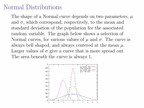
Normal Distributions
The shape of a Normal curve depends on two parameters, µand σ, which correspond, respectively, to the mean andstandard deviation of the population for the associatedrandom variable. The graph below shows a selection ofNormal curves, for various values of µ and σ. The curve isalways bell shaped, and always centered at the mean µ.Larger values of σ give a curve that is more spread out.The area beneath the curve is always 1.

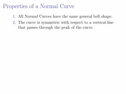
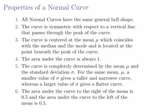
Properties of a Normal Curve
1. All Normal Curves have the same general bell shape.
2. The curve is symmetric with respect to a vertical linethat passes through the peak of the curve.
3. The curve is centered at the mean µ which coincideswith the median and the mode and is located at thepoint beneath the peak of the curve.
4. The area under the curve is always 1.
5. The curve is completely determined by the mean µ andthe standard deviation σ. For the same mean, µ, asmaller value of σ gives a taller and narrower curve,whereas a larger value of σ gives a flatter curve.
6. The area under the curve to the right of the mean is0.5 and the area under the curve to the left of themean is 0.5.
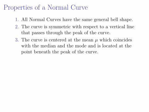
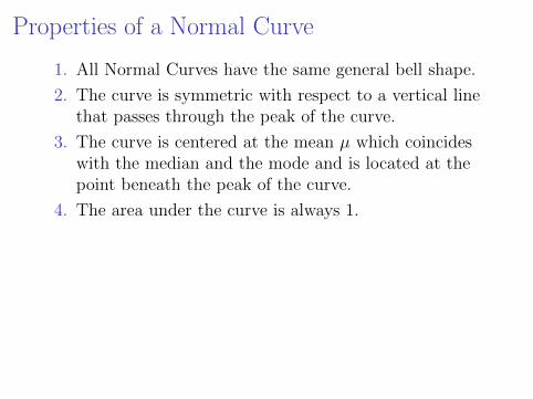
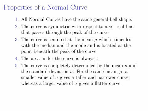

Properties of a Normal Curve
7. The empirical rule (68%, 95%, 99.7%) for moundshaped data applies to variables with normaldistributions.For example, approximately 95% of the measurementswill fall within 2 standard deviations of the mean, i.e.within the interval (µ− 2σ, µ+ 2σ).
8. If a random variable X associated to an experimenthas a normal probability distribution, the probabilitythat the value of X derived from a single trial of theexperiment is between two given values x1 and x2(P(x1 6 X 6 x2)) is the area under the associatednormal curve between x1 and x2. For any given valuex1, P(X = x1) = 0, soP(x1 6 X 6 x2) = P(x1 < X < x2).
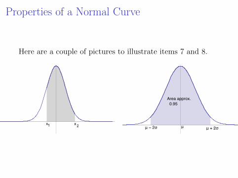
Properties of a Normal Curve
Here are a couple of pictures to illustrate items 7 and 8.
xx x1 2
Area approx. 0.95
μμ − 2σ μ + 2σ
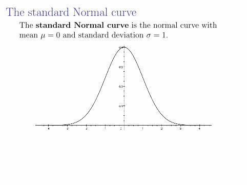
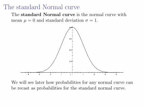
The standard Normal curveThe standard Normal curve is the normal curve withmean µ = 0 and standard deviation σ = 1.
We will see later how probabilities for any normal curve canbe recast as probabilities for the standard normal curve.
For the standard normal, probabilities are computed eitherby means of a computer/calculator of via a table.
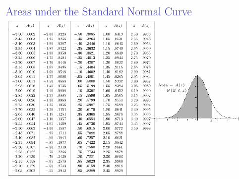
Areas under the Standard Normal Curve
z
Area = A(z)
= P(Z 6 z)

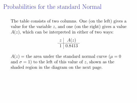
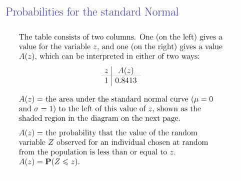
Probabilities for the standard Normal
The table consists of two columns. One (on the left) gives avalue for the variable z, and one (on the right) gives a valueA(z), which can be interpreted in either of two ways:
z A(z)1 0.8413
A(z) = the area under the standard normal curve (µ = 0and σ = 1) to the left of this value of z, shown as theshaded region in the diagram on the next page.
A(z) = the probability that the value of the randomvariable Z observed for an individual chosen at randomfrom the population is less than or equal to z.A(z) = P(Z 6 z).

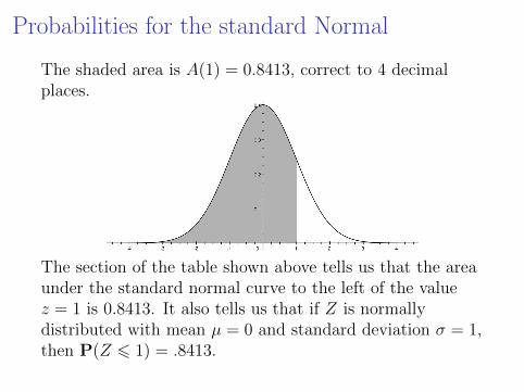
Probabilities for the standard Normal
The shaded area is A(1) = 0.8413, correct to 4 decimalplaces.
The section of the table shown above tells us that the areaunder the standard normal curve to the left of the valuez = 1 is 0.8413. It also tells us that if Z is normallydistributed with mean µ = 0 and standard deviation σ = 1,then P(Z 6 1) = .8413.
Examples
If Z is a standard normal random variable, what isP(Z 6 2)? Sketch the region under the standard normalcurve whose area is equal to P(Z 6 2). Use the table tofind P(Z 6 2).
P(Z 6 2) = 0.9772.

Examples
If Z is a standard normal random variable, what isP(Z 6 2)? Sketch the region under the standard normalcurve whose area is equal to P(Z 6 2). Use the table tofind P(Z 6 2).
P(Z 6 2) = 0.9772.
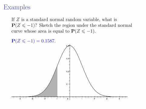
Examples
If Z is a standard normal random variable, what isP(Z 6 −1)? Sketch the region under the standard normalcurve whose area is equal to P(Z 6 −1).
P(Z 6 −1) = 0.1587.
Examples
If Z is a standard normal random variable, what isP(Z 6 −1)? Sketch the region under the standard normalcurve whose area is equal to P(Z 6 −1).
P(Z 6 −1) = 0.1587.
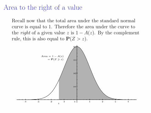
Area to the right of a value
Recall now that the total area under the standard normalcurve is equal to 1. Therefore the area under the curve tothe right of a given value z is 1− A(z). By the complementrule, this is also equal to P(Z > z).
z
Area = 1 − A(z)= P(Z > z)
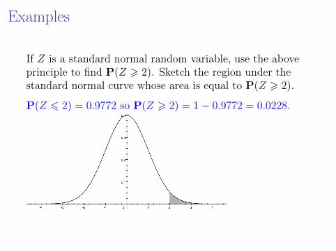
Examples
If Z is a standard normal random variable, use the aboveprinciple to find P(Z > 2). Sketch the region under thestandard normal curve whose area is equal to P(Z > 2).
P(Z 6 2) = 0.9772 so P(Z > 2) = 1− 0.9772 = 0.0228.
Examples
If Z is a standard normal random variable, use the aboveprinciple to find P(Z > 2). Sketch the region under thestandard normal curve whose area is equal to P(Z > 2).
P(Z 6 2) = 0.9772 so P(Z > 2) = 1− 0.9772 = 0.0228.
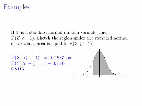
Examples
If Z is a standard normal random variable, findP(Z > −1). Sketch the region under the standard normalcurve whose area is equal to P(Z > −1).
P(Z 6 −1) = 0.1587 soP(Z > −1) = 1 − 0.1587 =0.8413.
Examples
If Z is a standard normal random variable, findP(Z > −1). Sketch the region under the standard normalcurve whose area is equal to P(Z > −1).
P(Z 6 −1) = 0.1587 soP(Z > −1) = 1 − 0.1587 =0.8413.
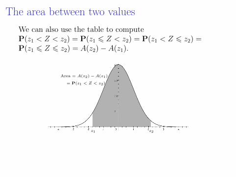
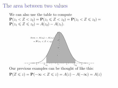
The area between two values
We can also use the table to computeP(z1 < Z < z2) = P(z1 6 Z < z2) = P(z1 < Z 6 z2) =P(z1 6 Z 6 z2) = A(z2)− A(z1).
z1 z2
Area = A(z2) − A(z1)
= P(z1 < Z < z2)
Our previous examples can be thought of like this:
P(Z 6 z) = P(−∞ < Z 6 z) = A(z)− A(−∞) = A(z)
P(z < Z) = P(z < Z <∞) = A(∞)− A(z) = 1− A(z)
Example
If Z is a standard normal random variable, findP(−3 6 Z 6 3). Sketch the region under the standardnormal curve whose area is equal to P(−3 6 Z 6 3).
P(−3 6 Z 6 3) = P(Z 6 3)−P(Z 6 −3) =0.9987− 0.0013 = 0.9973.

Example
If Z is a standard normal random variable, findP(−3 6 Z 6 3). Sketch the region under the standardnormal curve whose area is equal to P(−3 6 Z 6 3).
P(−3 6 Z 6 3) = P(Z 6 3)−P(Z 6 −3) =0.9987− 0.0013 = 0.9973.
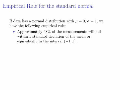
Empirical Rule for the standard normal
If data has a normal distribution with µ = 0, σ = 1, wehave the following empirical rule:
I Approximately 68% of the measurements will fallwithin 1 standard deviation of the mean orequivalently in the interval (−1, 1).
I Approximately 95% of the measurements will fallwithin 2 standard deviations of the mean orequivalently in the interval (−2, 2).
I Approximately 99.7% of the measurements (essentiallyall) will fall within 3 standard deviations of the mean,or equivalently in the interval (−3, 3).

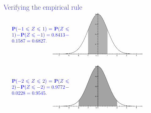
Verifying the empirical rule
P(−1 6 Z 6 1) = P(Z 61)−P(Z 6 −1) = 0.8413−0.1587 = 0.6827.
P(−2 6 Z 6 2) = P(Z 62)−P(Z 6 −2) = 0.9772−0.0228 = 0.9545.
Verifying the empirical rule
P(−1 6 Z 6 1) = P(Z 61)−P(Z 6 −1) = 0.8413−0.1587 = 0.6827.
P(−2 6 Z 6 2) = P(Z 62)−P(Z 6 −2) = 0.9772−0.0228 = 0.9545.

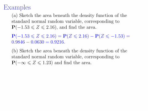
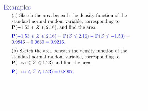
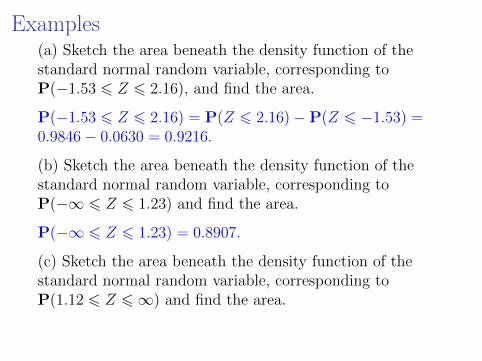
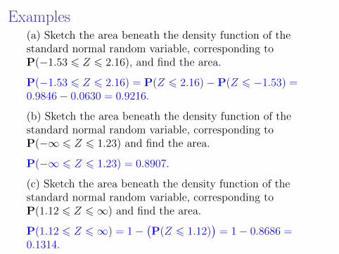
Examples(a) Sketch the area beneath the density function of thestandard normal random variable, corresponding toP(−1.53 6 Z 6 2.16), and find the area.
P(−1.53 6 Z 6 2.16) = P(Z 6 2.16)−P(Z 6 −1.53) =0.9846− 0.0630 = 0.9216.
(b) Sketch the area beneath the density function of thestandard normal random variable, corresponding toP(−∞ 6 Z 6 1.23) and find the area.
P(−∞ 6 Z 6 1.23) = 0.8907.
(c) Sketch the area beneath the density function of thestandard normal random variable, corresponding toP(1.12 6 Z 6∞) and find the area.
P(1.12 6 Z 6∞) = 1−(P(Z 6 1.12)
)= 1− 0.8686 =
0.1314.
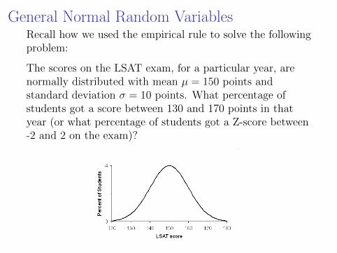
General Normal Random VariablesRecall how we used the empirical rule to solve the followingproblem:
The scores on the LSAT exam, for a particular year, arenormally distributed with mean µ = 150 points andstandard deviation σ = 10 points. What percentage ofstudents got a score between 130 and 170 points in thatyear (or what percentage of students got a Z-score between-2 and 2 on the exam)?
LSAT Scores distribution and US Law Schools http://www.studentdoc.com/lsat-scores.html
2 of 3 6/24/07 2:15 PM

General Normal Random VariablesLSAT Scores distribution and US Law Schools http://www.studentdoc.com/lsat-scores.html
2 of 3 6/24/07 2:15 PM
We will now use normal distribution tables to solve thiskind of problem. We do not have a table for every normalrandom variable (there are infinitely many of them!). So wewill convert problems about general normal random toproblems about the standard normal random variable, bystandardizing — converting all relevant values of thegeneral normal random variable to z-scores, and thencalculating probabilities of these z-scores from a standardnormal table (or using a calculator).

Standardizing
If X is a normal random variable with mean µ and standarddeviation σ, then the random variable Z defined by
Z =X − µσ
“z-score of Z”
has a standard normal distribution. The value of Z givesthe number of standard deviations between X and themean µ (negative values are values below the mean,positive values are values above the mean).
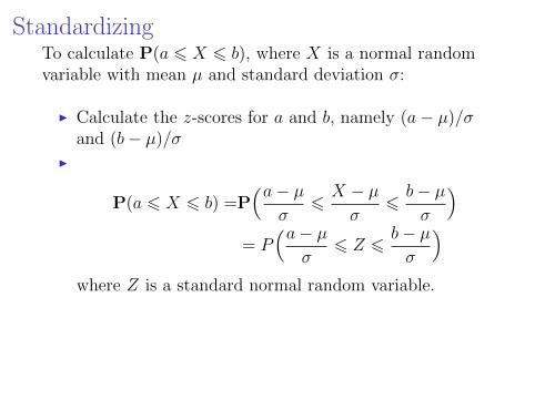
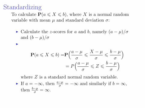
StandardizingTo calculate P(a 6 X 6 b), where X is a normal randomvariable with mean µ and standard deviation σ:
I Calculate the z-scores for a and b, namely (a− µ)/σand (b− µ)/σ
I
P(a 6 X 6 b) =P(a− µ
σ6X − µσ
6b− µσ
)= P
(a− µσ
6 Z 6b− µσ
)where Z is a standard normal random variable.
I If a = −∞, then a−µσ
= −∞ and similarly if b =∞,
then b−µσ
=∞.
I Use a table or a calculator for standard normalprobability distribution to calculate the probability.
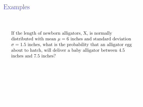
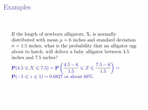
Examples
If the length of newborn alligators, X, is normallydistributed with mean µ = 6 inches and standard deviationσ = 1.5 inches, what is the probability that an alligator eggabout to hatch, will deliver a baby alligator between 4.5inches and 7.5 inches?
P(4.5 6 X 6 7.5) = P
(4.5− 6
1.56 Z 6
7.5− 6
1.5
)=
P(−1 6 z 6 1) = 0.6827 or about 68%.
Examples
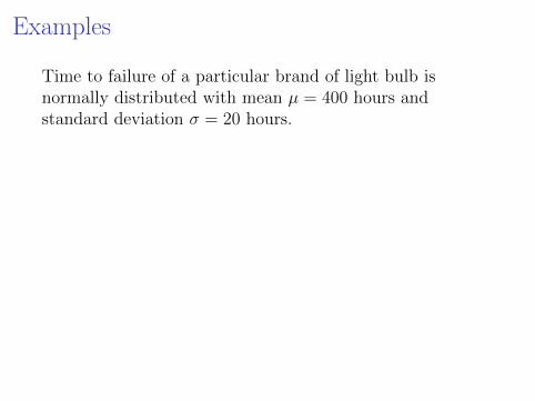
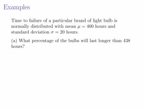
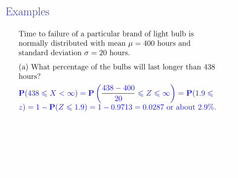
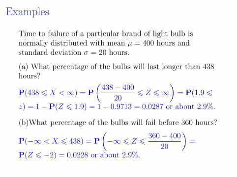
Time to failure of a particular brand of light bulb isnormally distributed with mean µ = 400 hours andstandard deviation σ = 20 hours.
(a) What percentage of the bulbs will last longer than 438hours?
P(438 6 X <∞) = P
(438− 400
206 Z 6∞
)= P(1.9 6
z) = 1−P(Z 6 1.9) = 1− 0.9713 = 0.0287 or about 2.9%.
(b)What percentage of the bulbs will fail before 360 hours?
P(−∞ < X 6 438) = P
(−∞ 6 Z 6
360− 400
20
)=
P(Z 6 −2) = 0.0228 or about 2.9%.
Examples
Time to failure of a particular brand of light bulb isnormally distributed with mean µ = 400 hours andstandard deviation σ = 20 hours.
(a) What percentage of the bulbs will last longer than 438hours?
P(438 6 X <∞) = P
(438− 400
206 Z 6∞
)= P(1.9 6
z) = 1−P(Z 6 1.9) = 1− 0.9713 = 0.0287 or about 2.9%.
(b)What percentage of the bulbs will fail before 360 hours?
P(−∞ < X 6 438) = P
(−∞ 6 Z 6
360− 400
20
)=
P(Z 6 −2) = 0.0228 or about 2.9%.
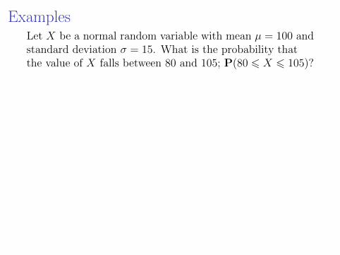
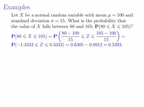
ExamplesLet X be a normal random variable with mean µ = 100 andstandard deviation σ = 15. What is the probability thatthe value of X falls between 80 and 105; P(80 6 X 6 105)?
P(80 6 X 6 105) = P
(80− 100
156 Z 6
105− 100
15
)=
P(−1.3333 6 Z 6 0.3333) = 0.6305− 0.0912 = 0.5393.
Example Dental Anxiety Assume that scores on aDental anxiety scale (ranging from 0 to 20) are normal forthe general population, with mean µ = 11 and standarddeviation σ = 3.5.
(a) What is the probability that a person chosen at randomwill score between 10 and 15 on this scale?
P(80 6 X 6 105) = P
(10− 11
3.56 Z 6
15− 11
3.5
)=
P(−0.2857 6 Z 6 1.1429) = 0.8735− 0.3875 = 0.4859.

Examples
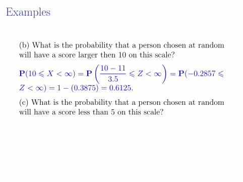
(b) What is the probability that a person chosen at randomwill have a score larger then 10 on this scale?
P(10 6 X <∞) = P
(10− 11
3.56 Z <∞
)= P(−0.2857 6
Z <∞) = 1− (0.3875) = 0.6125.
(c) What is the probability that a person chosen at randomwill have a score less than 5 on this scale?
P(−∞ < X 6 5) = P
(∞ < Z 6
5− 11
3.5
)= P(Z 6
−1.7143) = 0.0432.

Examples
(b) What is the probability that a person chosen at randomwill have a score larger then 10 on this scale?
P(10 6 X <∞) = P
(10− 11
3.56 Z <∞
)= P(−0.2857 6
Z <∞) = 1− (0.3875) = 0.6125.
(c) What is the probability that a person chosen at randomwill have a score less than 5 on this scale?
P(−∞ < X 6 5) = P
(∞ < Z 6
5− 11
3.5
)= P(Z 6
−1.7143) = 0.0432.
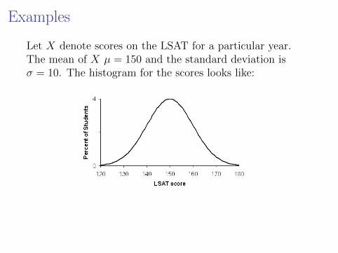
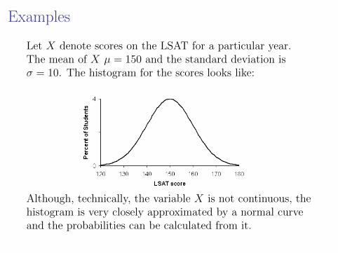
Examples
Let X denote scores on the LSAT for a particular year.The mean of X µ = 150 and the standard deviation isσ = 10. The histogram for the scores looks like:LSAT Scores distribution and US Law Schools http://www.studentdoc.com/lsat-scores.html
2 of 3 6/24/07 2:15 PM
Although, technically, the variable X is not continuous, thehistogram is very closely approximated by a normal curveand the probabilities can be calculated from it.
Examples
What percentage of students had a score of 165 or higheron this LSAT exam?
P(165 6 X <∞) = P
(165− 150
106 Z <∞
)= P(1.5 6
Z <∞) = 1−P(Z 6 1.5) = 1− (0.9332) = 0.0668.

Examples
What percentage of students had a score of 165 or higheron this LSAT exam?
P(165 6 X <∞) = P
(165− 150
106 Z <∞
)= P(1.5 6
Z <∞) = 1−P(Z 6 1.5) = 1− (0.9332) = 0.0668.

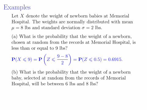
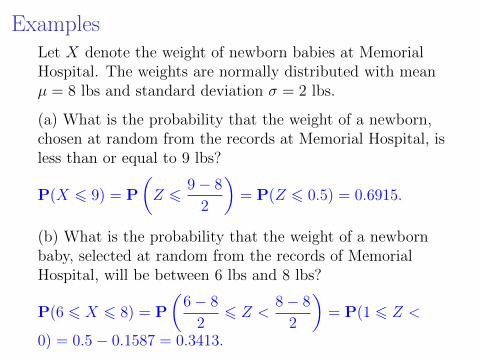
ExamplesLet X denote the weight of newborn babies at MemorialHospital. The weights are normally distributed with meanµ = 8 lbs and standard deviation σ = 2 lbs.
(a) What is the probability that the weight of a newborn,chosen at random from the records at Memorial Hospital, isless than or equal to 9 lbs?
P(X 6 9) = P
(Z 6
9− 8
2
)= P(Z 6 0.5) = 0.6915.
(b) What is the probability that the weight of a newbornbaby, selected at random from the records of MemorialHospital, will be between 6 lbs and 8 lbs?
P(6 6 X 6 8) = P
(6− 8
26 Z <
8− 8
2
)= P(1 6 Z <
0) = 0.5− 0.1587 = 0.3413.

Examples
Example Let X denote Miriam’s monthly living expenses.X is normally distributed with mean µ = $1, 000 andstandard deviation σ = $150. On Jan. 1, Miriam finds outthat her money supply for January is $1,150. What is theprobability that Miriam’s money supply will run out beforethe end of January?
If Miriam’s monthly expenses exceed $1, 150 she will runout of money before the end of the month. Hence we want
P(1, 150 6 X): P
(1150− 1000
1506 X
)= P(1 6 Z) =
1−P(Z 6 1) = 1− (0.8413) = 0.1587.
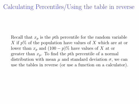
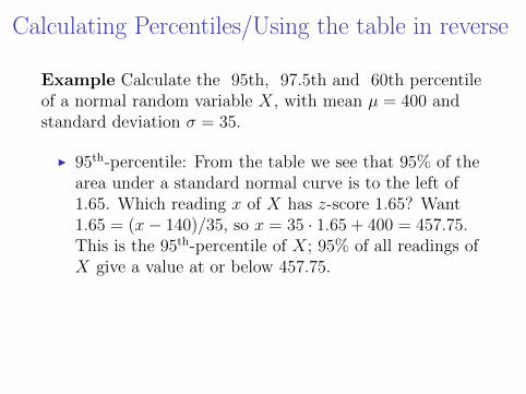
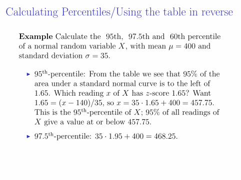
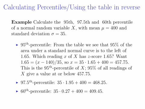
Calculating Percentiles/Using the table in reverse
Recall that xp is the pth percentile for the random variableX if p% of the population have values of X which are at orlower than xp and (100− p)% have values of X at orgreater than xp. To find the pth percentile of a normaldistribution with mean µ and standard deviation σ, we canuse the tables in reverse (or use a function on a calculator).
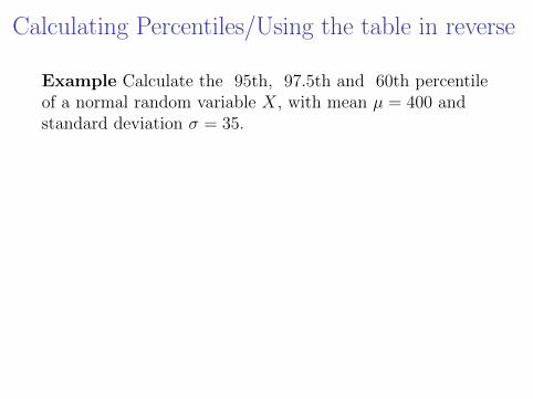
Calculating Percentiles/Using the table in reverse
Example Calculate the 95th, 97.5th and 60th percentileof a normal random variable X, with mean µ = 400 andstandard deviation σ = 35.
I 95th-percentile: From the table we see that 95% of thearea under a standard normal curve is to the left of1.65. Which reading x of X has z-score 1.65? Want1.65 = (x− 140)/35, so x = 35 · 1.65 + 400 = 457.75.This is the 95th-percentile of X; 95% of all readings ofX give a value at or below 457.75.
I 97.5th-percentile: 35 · 1.95 + 400 = 468.25.
I 60th-percentile: 35 · 0.27 + 400 = 409.45.
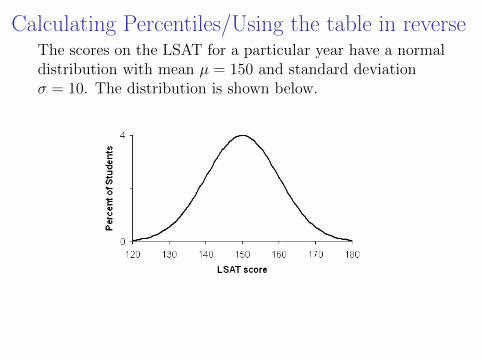
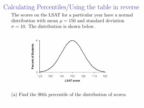
Calculating Percentiles/Using the table in reverseThe scores on the LSAT for a particular year have a normaldistribution with mean µ = 150 and standard deviationσ = 10. The distribution is shown below.
LSAT Scores distribution and US Law Schools http://www.studentdoc.com/lsat-scores.html
2 of 3 6/24/07 2:15 PM
(a) Find the 90th percentile of the distribution of scores.
90th-percentile a = 162.8155.
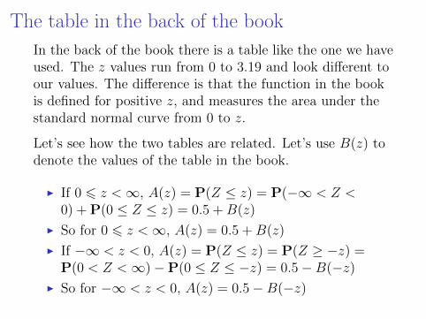
The table in the back of the book
In the back of the book there is a table like the one we haveused. The z values run from 0 to 3.19 and look different toour values.
The difference is that the function in the bookis defined for positive z, and measures the area under thestandard normal curve from 0 to z.
Let’s see how the two tables are related. Let’s use B(z) todenote the values of the table in the book.
I If 0 6 z <∞, A(z) = P(Z ≤ z) = P(−∞ < Z <0) + P(0 ≤ Z ≤ z) = 0.5 +B(z)
I So for 0 6 z <∞, A(z) = 0.5 +B(z)
I If −∞ < z < 0, A(z) = P(Z ≤ z) = P(Z ≥ −z) =P(0 < Z <∞)−P(0 ≤ Z ≤ −z) = 0.5−B(−z)
I So for −∞ < z < 0, A(z) = 0.5−B(−z)

The table in the back of the book
In the back of the book there is a table like the one we haveused. The z values run from 0 to 3.19 and look different toour values. The difference is that the function in the bookis defined for positive z, and measures the area under thestandard normal curve from 0 to z.
Let’s see how the two tables are related. Let’s use B(z) todenote the values of the table in the book.
I If 0 6 z <∞, A(z) = P(Z ≤ z) = P(−∞ < Z <0) + P(0 ≤ Z ≤ z) = 0.5 +B(z)
I So for 0 6 z <∞, A(z) = 0.5 +B(z)
I If −∞ < z < 0, A(z) = P(Z ≤ z) = P(Z ≥ −z) =P(0 < Z <∞)−P(0 ≤ Z ≤ −z) = 0.5−B(−z)
I So for −∞ < z < 0, A(z) = 0.5−B(−z)
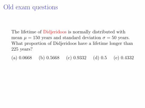
Old exam questions
The lifetime of Didjeridoos is normally distributed withmean µ = 150 years and standard deviation σ = 50 years.What proportion of Didjeridoos have a lifetime longer than225 years?
(a) 0.0668 (b) 0.5668 (c) 0.9332 (d) 0.5 (e) 0.4332
P(225 6 X) = P
(225− 150
506 Z
)= P(1.5 6 Z) =
1−P(Z 6 1.5) = 1− 0.9332 = 0.0668.
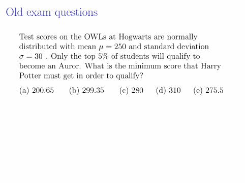
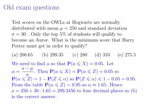
Old exam questions
Test scores on the OWLs at Hogwarts are normallydistributed with mean µ = 250 and standard deviationσ = 30 . Only the top 5% of students will qualify tobecome an Auror. What is the minimum score that HarryPotter must get in order to qualify?
(a) 200.65 (b) 299.35 (c) 280 (d) 310 (e) 275.5
We need to find a so that P(a 6 X) = 0.05. Let
α =a− µσ
. Then P(a 6 X) = P(α 6 Z) = 0.05 so
P(α 6 Z) = 1−P(Z 6 α) so P(Z 6 α) 6 1− 0.05 = 0.95.From the table P(α 6 Z) = 0.95 so α ≈ 1.65. Hencea = 250 + 30 · 1.65 = 299.3456 to four decimal places so (b)is the correct answer.
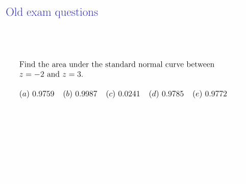
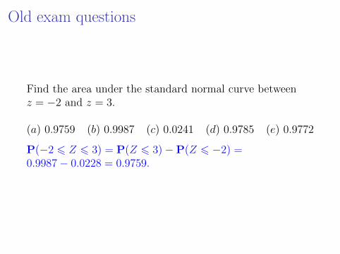
Old exam questions
Find the area under the standard normal curve betweenz = −2 and z = 3.
(a) 0.9759 (b) 0.9987 (c) 0.0241 (d) 0.9785 (e) 0.9772
P(−2 6 Z 6 3) = P(Z 6 3)−P(Z 6 −2) =0.9987− 0.0228 = 0.9759.
Old exam questions
Find the area under the standard normal curve betweenz = −2 and z = 3.
(a) 0.9759 (b) 0.9987 (c) 0.0241 (d) 0.9785 (e) 0.9772
P(−2 6 Z 6 3) = P(Z 6 3)−P(Z 6 −2) =0.9987− 0.0228 = 0.9759.

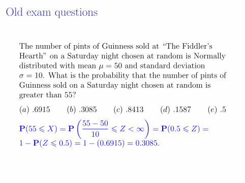
Old exam questions
The number of pints of Guinness sold at “The Fiddler’sHearth” on a Saturday night chosen at random is Normallydistributed with mean µ = 50 and standard deviationσ = 10. What is the probability that the number of pints ofGuinness sold on a Saturday night chosen at random isgreater than 55?
(a) .6915 (b) .3085 (c) .8413 (d) .1587 (e) .5
P(55 6 X) = P
(55− 50
106 Z <∞
)= P(0.5 6 Z) =
1−P(Z 6 0.5) = 1− (0.6915) = 0.3085.
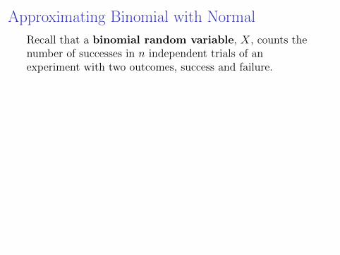
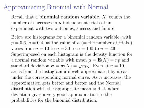
Approximating Binomial with Normal
Recall that a binomial random variable, X, counts thenumber of successes in n independent trials of anexperiment with two outcomes, success and failure.
Below are histograms for a binomial random variable, withp = 0.6, q = 0.4, as the value of n (= the number of trials )varies from n = 10 to n = 30 to n = 100 to n = 200.Superimposed on each histogram is the density function fora normal random variable with mean µ = E(X) = np andstandard deviation σ = σ(X) =
√npq. Even at n = 10,
areas from the histogram are well approximated by areasunder the corresponding normal curve. As n increases, theapproximation gets better and better and the Normaldistribution with the appropriate mean and standarddeviation gives a very good approximation to theprobabilities for the binomial distribution.
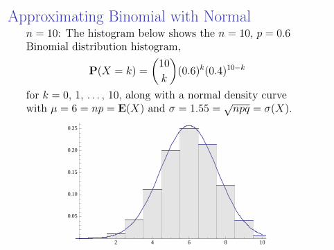
Approximating Binomial with Normaln = 10: The histogram below shows the n = 10, p = 0.6Binomial distribution histogram,
P(X = k) =
(10
k
)(0.6)k(0.4)10−k
for k = 0, 1, . . . , 10, along with a normal density curvewith µ = 6 = np = E(X) and σ = 1.55 =
√npq = σ(X).
2 4 6 8 10
0.05
0.10
0.15
0.20
0.25
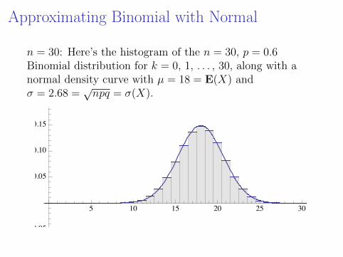
Approximating Binomial with Normal
n = 30: Here’s the histogram of the n = 30, p = 0.6Binomial distribution for k = 0, 1, . . . , 30, along with anormal density curve with µ = 18 = E(X) andσ = 2.68 =
√npq = σ(X).
5 10 15 20 25 30
-0.10
-0.05
0.05
0.10
0.15
0.20
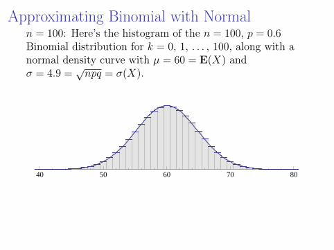
Approximating Binomial with Normaln = 100: Here’s the histogram of the n = 100, p = 0.6Binomial distribution for k = 0, 1, . . . , 100, along with anormal density curve with µ = 60 = E(X) andσ = 4.9 =
√npq = σ(X).
40 50 60 70 80

Approximating Binomial with Normaln = 200: Finally, here’s the histogram of the n = 200,p = 0.6 Binomial distribution for k = 0, 1, . . . , 200, alongwith a normal density curve with µ = 120 = E(X) andσ = 6.93 =
√npq = σ(X).
90 100 110 120 130 140 150

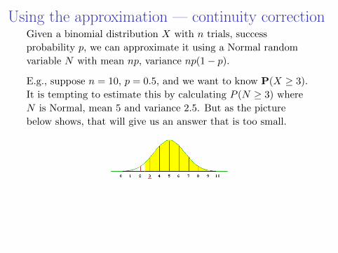
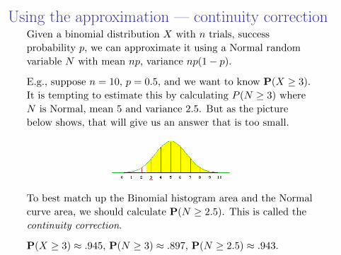
Using the approximation — continuity correctionGiven a binomial distribution X with n trials, success
probability p, we can approximate it using a Normal random
variable N with mean np, variance np(1− p).
E.g., suppose n = 10, p = 0.5, and we want to know P(X ≥ 3).
It is tempting to estimate this by calculating P (N ≥ 3) where
N is Normal, mean 5 and variance 2.5. But as the picture
below shows, that will give us an answer that is too small.
To best match up the Binomial histogram area and the Normal
curve area, we should calculate P(N ≥ 2.5). This is called the
continuity correction.
P(X ≥ 3) ≈ .945, P(N ≥ 3) ≈ .897, P(N ≥ 2.5) ≈ .943.
Continuity correction
Given a binomial distribution X with n trials, successprobability p, we can approximate it using a Normalrandom variable N with mean np, variance np(1− p).
The continuity correction tells us that when we move fromX to N , we should make the following changes to theprobabilities we are calculating:
I X ≥ a changes to N ≥ a− 0.5
I X > a changes to N ≥ a+ 0.5
I X ≤ a changes to N ≤ a+ 0.5
I X < a changes to N ≤ a− 0.5

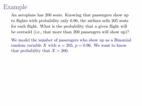
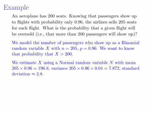
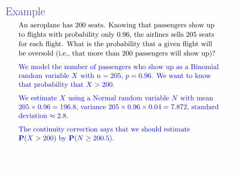
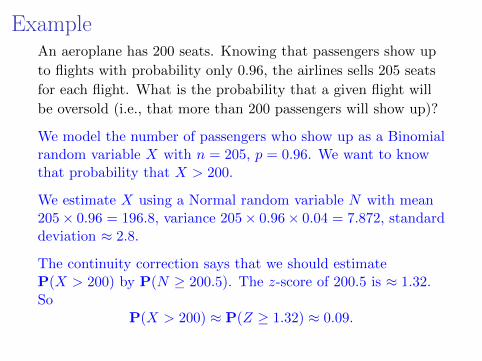
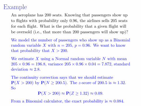
ExampleAn aeroplane has 200 seats. Knowing that passengers show up
to flights with probability only 0.96, the airlines sells 205 seats
for each flight. What is the probability that a given flight will
be oversold (i.e., that more than 200 passengers will show up)?
We model the number of passengers who show up as a Binomialrandom variable X with n = 205, p = 0.96. We want to knowthat probability that X > 200.
We estimate X using a Normal random variable N with mean205× 0.96 = 196.8, variance 205× 0.96× 0.04 = 7.872, standarddeviation ≈ 2.8.
The continuity correction says that we should estimateP(X > 200) by P(N ≥ 200.5). The z-score of 200.5 is ≈ 1.32.So
P(X > 200) ≈ P(Z ≥ 1.32) ≈ 0.09.
From a Binomial calculator, the exact probability is ≈ 0.084.
ExampleAn aeroplane has 200 seats. Knowing that passengers show up
to flights with probability only 0.96, the airlines sells 205 seats
for each flight. What is the probability that a given flight will
be oversold (i.e., that more than 200 passengers will show up)?
We model the number of passengers who show up as a Binomialrandom variable X with n = 205, p = 0.96. We want to knowthat probability that X > 200.
We estimate X using a Normal random variable N with mean205× 0.96 = 196.8, variance 205× 0.96× 0.04 = 7.872, standarddeviation ≈ 2.8.
The continuity correction says that we should estimateP(X > 200) by P(N ≥ 200.5).
The z-score of 200.5 is ≈ 1.32.So
P(X > 200) ≈ P(Z ≥ 1.32) ≈ 0.09.
From a Binomial calculator, the exact probability is ≈ 0.084.
ExampleAn aeroplane has 200 seats. Knowing that passengers show up
to flights with probability only 0.96, the airlines sells 205 seats
for each flight. What is the probability that a given flight will
be oversold (i.e., that more than 200 passengers will show up)?
We model the number of passengers who show up as a Binomialrandom variable X with n = 205, p = 0.96. We want to knowthat probability that X > 200.
We estimate X using a Normal random variable N with mean205× 0.96 = 196.8, variance 205× 0.96× 0.04 = 7.872, standarddeviation ≈ 2.8.
The continuity correction says that we should estimateP(X > 200) by P(N ≥ 200.5). The z-score of 200.5 is ≈ 1.32.So
P(X > 200) ≈ P(Z ≥ 1.32) ≈ 0.09.
From a Binomial calculator, the exact probability is ≈ 0.084.
ExampleAn aeroplane has 200 seats. Knowing that passengers show up
to flights with probability only 0.96, the airlines sells 205 seats
for each flight. What is the probability that a given flight will
be oversold (i.e., that more than 200 passengers will show up)?
We model the number of passengers who show up as a Binomialrandom variable X with n = 205, p = 0.96. We want to knowthat probability that X > 200.
We estimate X using a Normal random variable N with mean205× 0.96 = 196.8, variance 205× 0.96× 0.04 = 7.872, standarddeviation ≈ 2.8.
The continuity correction says that we should estimateP(X > 200) by P(N ≥ 200.5). The z-score of 200.5 is ≈ 1.32.So
P(X > 200) ≈ P(Z ≥ 1.32) ≈ 0.09.
From a Binomial calculator, the exact probability is ≈ 0.084.

Polling example I
Melinda McNulty is running for the city council this May,with one opponent, Mark Reckless. She needs to get morethan 50% of the votes to win.
I take a random sample of 100 people and ask them if theywill vote for Melinda or not. Now assuming the populationis large, the variable X = number of people who say “yes”has a distribution which is basically a binomial distributionwith n = 100.
We do not know what p is. Suppose that in our poll, wefound that 40% of the sample say that they will vote forMelinda. This is not good news, as it suggests p ≈ .4, butthis may be just due to variation in sample statistics.
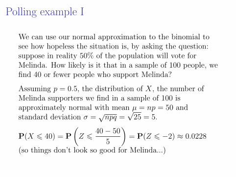
Polling example I
We can use our normal approximation to the binomial tosee how hopeless the situation is, by asking the question:suppose in reality 50% of the population will vote forMelinda. How likely is it that in a sample of 100 people, wefind 40 or fewer people who support Melinda?
Assuming p = 0.5, the distribution of X, the number ofMelinda supporters we find in a sample of 100 isapproximately normal with mean µ = np = 50 andstandard deviation σ =
√npq =
√25 = 5.
P(X 6 40) = P
(Z 6
40− 50
5
)= P(Z 6 −2) ≈ 0.0228
(so things don’t look so good for Melinda...)
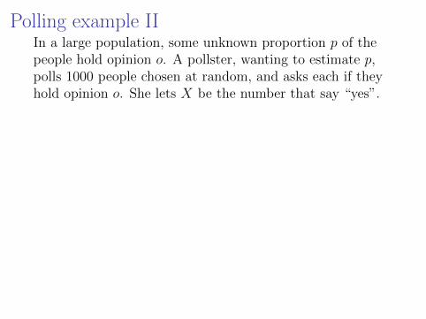
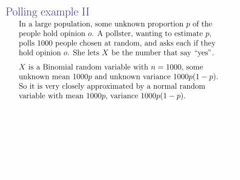
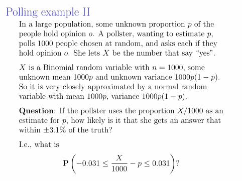
Polling example IIIn a large population, some unknown proportion p of thepeople hold opinion o. A pollster, wanting to estimate p,polls 1000 people chosen at random, and asks each if theyhold opinion o. She lets X be the number that say “yes”.
X is a Binomial random variable with n = 1000, someunknown mean 1000p and unknown variance 1000p(1− p).So it is very closely approximated by a normal randomvariable with mean 1000p, variance 1000p(1− p).
Question: If the pollster uses the proportion X/1000 as anestimate for p, how likely is it that she gets an answer thatwithin ±3.1% of the truth?
I.e., what is
P
(−0.031 ≤ X
1000− p ≤ 0.031
)?

Polling example IIP(−0.031 ≤ X
1000−p ≤ 0.031) = P(1000p−31 ≤ X ≤ 1000p+31)
z-score of 1000p− 31 is −31√1000p(1−p)
≈ −0.98√p(1−p)
.
z-score of 1000p− 31 is 31√1000p(1−p)
≈ 0.98√p(1−p)
.
So P(−0.031 ≤ X1000 − p ≤ 0.031) ≈ P( −0.98√
p(1−p)≤ Z ≤ 0.98√
p(1−p))
P( −0.98√p(1−p)
≤ Z ≤ 0.98√p(1−p)
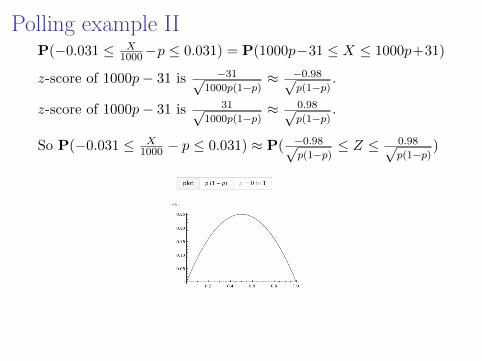
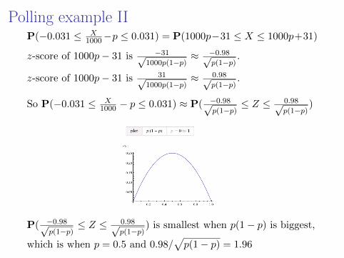
) is smallest when p(1− p) is biggest,
which is when p = 0.5 and 0.98/√p(1− p) = 1.96
Polling example IIP(−0.031 ≤ X
1000−p ≤ 0.031) = P(1000p−31 ≤ X ≤ 1000p+31)
z-score of 1000p− 31 is −31√1000p(1−p)
≈ −0.98√p(1−p)
.
z-score of 1000p− 31 is 31√1000p(1−p)
≈ 0.98√p(1−p)
.
So P(−0.031 ≤ X1000 − p ≤ 0.031) ≈ P( −0.98√
p(1−p)≤ Z ≤ 0.98√
p(1−p))
P( −0.98√p(1−p)
≤ Z ≤ 0.98√p(1−p)
) is smallest when p(1− p) is biggest,
which is when p = 0.5 and 0.98/√p(1− p) = 1.96

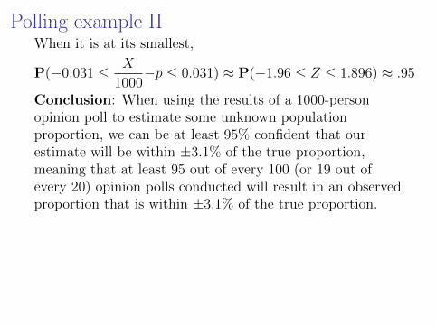
Polling example IIWhen it is at its smallest,
P(−0.031 ≤ X
1000−p ≤ 0.031) ≈ P(−1.96 ≤ Z ≤ 1.896) ≈ .95
Conclusion: When using the results of a 1000-personopinion poll to estimate some unknown populationproportion, we can be at least 95% confident that ourestimate will be within ±3.1% of the true proportion,meaning that at least 95 out of every 100 (or 19 out ofevery 20) opinion polls conducted will result in an observedproportion that is within ±3.1% of the true proportion.
I But 1 out of every 20 polls will be wrong!
I ±3.1% is called the “margin or error”
I All this assumes that the polling was done randomly
I Works regardless of the size of the population being polled