norm-based capacity control in neural networksproceedings.mlr.press/v40/neyshabur15.pdf ·...

JMLR: Workshop and Conference Proceedings vol 40:1–26, 2015

Norm-Based Capacity Control in Neural Networks

Behnam Neyshabur [email protected]

Ryota Tomioka [email protected]

Nathan Srebro [email protected]

Toyota Technological Institute at Chicago, Chicago, IL 60637, USA

AbstractWe investigate the capacity, convexity and characterization of a general family of norm-constrainedfeed-forward networks.Keywords: Feed-forward neural networks, deep learning, scale-sensitive capacity control

1. Introduction

The statistical complexity, or capacity, of unregularized feed-forward neural networks, as a functionof the network size and depth, is fairly well understood. With hard-threshold activations, the VC-dimension, and hence sample complexity, of the class of functions realizable with a feed-forwardnetwork is equal, up to logarithmic factors, to the number of edges in the network (Anthony andBartlett, 2009; Shalev-Shwartz and Ben-David, 2014), corresponding to the number of parameters.With continuous activation functions the VC-dimension could be higher, but is fairly well under-stood and is still controlled by the size and depth of the network.1

But feedforward networks are often trained with some kind of explicit or implicit regularization,such as weight decay, early stopping, “max regularization”, or more exotic regularization such asdrop-outs. What is the effect of such regularization on the induced hypothesis class and its capacity?

For linear prediction (a one-layer feed-forward network) we know that using regularization thecapacity of the class can be bounded only in terms of the norms, with no (or a very weak) depen-dence on the number of edges (i.e. the input dimensionality or number of linear coefficients). E.g.,we understand very well how the capacity of `2-regularized linear predictors can be bounded interms of the norm alone (when the norm of the data is also bounded), even in infinite dimension.

A central question we ask is: can we bound the capacity of feed-forward network in termsof norm-based regularization alone, without relying on network size and even if the network size(number of nodes or edges) is unbounded or infinite? What type of regularizers admit such capacitycontrol? And how does the capacity behave as a function of the norm, and perhaps other networkparameters such as depth?

Beyond the central question of capacity control, we also analyze the convexity of the resultinghypothesis class—unlike unregularized size-controlled feed-forward networks, infinite magnitude-controlled networks have the potential of yielding convex hypothesis classes (this is the case, e.g.,

1. Using weights with very high precision and vastly different magnitudes it is possible to shatter a number of pointsquadratic in the number of edges when activations such as the sigmoid, ramp or hinge are used (Shalev-Shwartz andBen-David, 2014, Chapter 20.4). But even with such activations, the VC dimension can still be bounded by the sizeand depth (Bartlett, 1998; Anthony and Bartlett, 2009; Shalev-Shwartz and Ben-David, 2014).

c© 2015 B. Neyshabur, R. Tomioka & N. Srebro.

NEYSHABUR TOMIOKA SREBRO

when we move from rank-based control on matrices, which limits the number of parameters tomagnitude based control with the trace-norm or max-norm). A convex class might be easier tooptimize over and might be convenient in other ways.

In this paper we focus on networks with rectified linear units and two natural types of norm reg-ularization: bounding the norm of the incoming weights of each unit (per-unit regularization) andbounding the overall norm of all the weights in the system jointly (overall regularization, e.g. lim-iting the overall sum of the magnitudes, or square magnitudes, in the system). We generalize bothof these with a single notion of group-norm regularization: we take the `p norm over the weightsin each unit and then the `q norm over units. In Section 3 we present this regularizer and obtaina tight understanding of when it provides for size-independent capacity control and a characteri-zation of when it induces convexity. We then apply these generic results to per-unit regularization(Section 4) and overall regularization (Section 5), noting also other forms of regularization that areequivalent to these two. In particular, we show how per-unit regularization is equivalent to a novelpath-based regularizer and how overall `2 regularization for two-layer networks is equivalent to so-called “convex neural networks” (Bengio et al., 2005). In terms of capacity control, we show thatper-unit regularization allows size-independent capacity-control only with a per-unit `1-norm, andthat overall `p regularization allows for size-independent capacity control only when p ≤ 2, even ifthe depth is bounded. In any case, even if we bound the sum of all magnitudes in the system, weshow that an exponential dependence on the depth is unavoidable.

As far as we are aware, prior work on size-independent capacity control for feed-forward net-works considered only per-unit `1 regularization, and per-unit `2 regularization for two-layerednetworks (see discussion and references at the beginning of Section 4). Here, we extend the scopesignificantly, and provide a broad characterization of the types of regularization possible and theirproperties. In particular, we consider overall norm regularization, which is perhaps the most naturalform of regularization used in practice (e.g. in the form of weight decay). We hope our study will beuseful in thinking about, analyzing and designing learning methods using feed-forward networks.Another motivation for us is that complexity of large-scale optimization is often related to scale-based, not dimension-based complexity. Understanding when the scale-based complexity dependsexponentially on the depth of a network might help shed light on understanding the difficulties inoptimizing deep networks.

2. Preliminaries: Feedforward Neural Networks

A feedforward neural network that computes a function f : RD → R is specified by a directedacyclic graph (DAG) G(V,E) with D special “input nodes” vin[1], . . . , vin[D] ∈ V with no incom-ing edges and a special “output node” vout ∈ V with no outgoing edges, weights w :E → R on theedges, and an activation function σ :R→ R.

Given an input x ∈ RD, the output values of the input units are set to the coordinates of x,o(vin[i]) = x[i] (we might want to also add a special “bias” node with o(vin[0]) = 1, or just rely onthe inputs having a fixed “bias coordinate”), the output value of internal nodes (all nodes except theinput and output nodes) are defined according to the forward propagation equation:

o(v) = σ

∑(u→v)∈E

w(u→ v)o(u)

, (1)

2

NORM-BASED CAPACITY CONTROL IN NEURAL NETWORKS

and the output value of the output unit is defined as o(vout) =∑

(u→vout)∈E w(u → vout)o(u). Thenetwork is then said to compute the function fG,w,σ(x) = o(vout). Given a graphs G and activationfunction σ, we can consider the hypothesis class of functionsNG,σ = fG,w,σ :RD → R | w :E →R computable using some setting of the weights.

We will refer to the size of the network, which is the overall number of edges |E|, the depth dof the network, which is the length of the longest directed path in G, and the in-degree (or width)H of a network, which is the maximum in-degree of a vertex in G.

A special case of feedforward neural networks are layered fully connected networks wherevertices are partitioned into layers and there is a directed edge from every vertex in layer i to everyvertex in layer i + 1. We index the layers from the first layer, i = 1 whose inputs are the inputnodes, up to the last layer i = d which contains the single output node—the number of layers isthus equal to the depth and the in-degree is the maximal layer size. We denote by layer(d,H) thelayered fully connected network with d layers and H nodes per layer (except the output layer thathas a single node), and also allow H =∞. We will also use the shorthand N d,H,σ = N layer(d,H),σ

and N d,σ = N layer(d,∞),σ.Layered networks can be parametrized by a sequence of matrices W1 ∈ RH×D,W2,

W3, . . . ,Wd−1 ∈ RH×H ,Wd ∈ R1×H where the row Wi[j, :] contains the input weights to unitj in layer i, and

fW (x) = Wdσ(Wd−1σ(Wd−2(. . . σ(W1x)))), (2)

where σ is applied element-wise.We will focus mostly on the hinge, or RELU (REctified Linear Unit) activation, which is

currently in popular use (Nair and Hinton, 2010; Bordes and Bengio, 2011; Zeiler et al., 2013),σRELU(z) = [z]+ = max(z, 0). When the activation will not be specified, we will implicitly bereferring to the RELU. The RELU has several convenient properties which we will exploit, some ofthem shared with other activation functions:

Lipshitz The hinge is Lipschitz continuous with Lipshitz constant one. This property is also sharedby the sigmoid and the ramp activation σ(z) = min(max(0, z), 1).

Idempotency The hinge is idempotent, i.e. σRELU(σRELU(z)) = σRELU(z). This property is alsoshared by the ramp and hard threshold activations.

Non-Negative Homogeneity For a non-negative scalar c ≥ 0 and any input z ∈ R we haveσRELU(c · z) = c · σRELU(z). This property is important as it allows us to scale the incom-ing weights to a unit by c > 0 and scale the outgoing edges by 1/c without changing the thefunction computed by the network. For layered graphs, this means we can scale Wi by c andcompensate by scaling Wi+1 by 1/c.

We will consider various measures α(w) of the magnitude of the weights w(·). Such a measureinduces a complexity measure on functions f ∈ NG,σ defined by αG,σ(f) = inffG,w,σ=f α(w).The sublevel sets of the complexity measure αG,σ form a family of hypothesis classes NG,σ

α≤a =

f ∈ NG,σ | αG,σ(f) ≤ a. Again we will use the shorthand αd,H,σ and αd,σ when referringto layered graphs layer(d,H) and layer(d,∞) respectively, and frequently drop σ when RELU isimplicitly meant.

For binary function g : ±1D → ±1 we say that g is realized by f with unit margin if∀xf(x)g(x) ≥ 1. A set of points S is shattered with unit margin by a hypothesis class N if allg : S → ±1 can be realized with unit margin by some f ∈ N .

3


3. Group Norm Regularization

Considering the grouping of weights going into each node of the network, we will consider thefollowing generic group-norm type regularizer, parametrized by 1 ≤ p, q ≤ ∞:

µp,q(w) =

∑v∈V

∑(u→v)∈E

|w(u→ v)|pq/p

1/q

. (3)

Here and elsewhere we allow q = ∞ with the usual conventions that (∑zqi )

1/q = sup zi and1/q = 0 when it appears in other contexts. When q = ∞ the group regularizer (3) imposes a per-unit regularization, where we constrain the norm of the incoming weights of each unit separately,and when q = p the regularizer (3) is an “overall” weight regularizer, constraining the overall normof all weights in the system. E.g., when q = p = 1 we are paying for the sum of all magnitudes ofweights in the network, and q = p = 2 corresponds to overall weight-decay where we pay for thesum of square magnitudes of all weights (i.e. the overall Euclidean norm of the weights).

For a layered graph, we have:

µp,q(W ) =

d∑k=1

H∑i=1

H∑j=1

|Wk[i, j]|pq/p

1/q

= d1/q

(1

d

d∑k=1

‖Wk‖qp,q

)1/q

≥ d1/q(

d∏k=1

‖Wk‖p,q

)1/d

, d1/q d

√γp,q(W ) (4)

where γp,q(W ) =d∏

k=1

‖Wk‖p,q aggregates the layers by multiplication instead of summation. The

inequality (4) holds regardless of the activation function, and so for any σ we have:

γd,H,σp,q (f) ≤(µd,H,σ(f)p,q

d1/q

)d. (5)

But due to the homogeneity of the RELU activation, when this activation is used we can alwaysbalance the norm between the different layers without changing the computed function so as toachieve equality in (4):

Claim 1 For any f ∈ N d,H,σRELU , µd,H,σRELUp,q (f) = d1/q

d

√γd,H,σRELUp,q (f).

Proof Let W be weights that realizes f and are optimal with respect to γp,g; i.e. γp,q(W ) =

γd,Hp,q (f). Let Wk = d√γp,q(W )Wk/ ‖Wk‖p,q, and observe that they also realize f . We now have:

µd,Hp,q (f) ≤ µp,q(W ) =(∑d

k=1

∥∥∥Wk

∥∥∥qp,q

)1/q=(d(γp,q(W )

)q/d)1/q= d1/q

d

√γd,H,σRELUp,q (f)

which together with (4) completes the proof.

The two measures are therefore equivalent when we use RELUs, and define the same level sets, orfamily of hypothesis classes, which we refer to simply as N d,H

p,q . In the remainder of this Section,we investigate convexity and generalization properties of these hypothesis classes.

4


3.1. Generalization and Capacity

In order to understand the effect of the norm on the sample complexity, we bound the Rademachercomplexity of the classesN d,H

p,q . Recall that the Rademacher Complexity is a measure of the capac-ity of a hypothesis class on a specific sample, which can be used to bound the difference betweenempirical and expected error, and thus the excess generalization error of empirical risk minimization(see, e.g., Bartlett and Mendelson (2003) for a complete treatment, and Appendix A for the exactdefinitions we use). In particular, the Rademacher complexity typically scales as

√C/m, which

corresponds to a sample complexity of O(C/ε2), where m is the sample size and C is the effectivemeasure of capacity of the hypothesis class.

Theorem 1 For any d, q ≥ 1, any 1 ≤ p <∞ and any set S = x1, . . . , xm ⊆ RD:

Rm(N d,H,σRELU

γp,q≤γ ) ≤ γ(

2H[ 1p∗−

1q]+)(d−1)

Rlinearm,p,D

≤

√√√√γ2(

2H[ 1p∗−

1q]+)2(d−1)

minp∗, 4 log(2D)maxi ‖xi‖2p∗m

and so:

Rm(N d,H,σRELU

µp,q≤µ ) ≤ µd(

2H[ 1p∗−

1q]+/

q√d)(d−1)

Rlinearm,p,D

≤

√√√√µ2d(

2H[ 1p∗−

1q]+/ q√d)2(d−1)


where the second inequalities hold only if 1 ≤ p ≤ 2, Rlinearm,p,D is the Rademacher complexity of

D-dimensional linear predictors with unit `p norm with respect to a set of m samples and p∗ is suchthat 1

p∗ + 1p = 1.

Proof sketch We prove the bound by induction, showing that for any q, d > 1 and 1 ≤ p <∞,

Rm(N d,H,σRELU

γp,q≤γ ) ≤ 2H[ 1p∗−

1q]+Rm(N d−1,H,σRELU

γp,q≤γ ).

The intuition is that when p∗ < q, the Rademacher complexity increases by simply distributing theweights among neurons and if p∗ ≥ q then the supremum is attained when the output neuron isconnected to a neuron with highest Rademacher complexity in the lower layer and all other weightsin the top layer are set to zero. For a complete proof, see Appendix A.

Note that for 2 ≤ p <∞, the bound on the Rademacher complexity scales withm1p (see section

A.1 in appendix) because:

Rlinearm,p,D ≤

√2 ‖X‖2,p∗m

≤√

2 maxi ‖xi‖p∗

m1p

(6)

The bound in Theorem 1 depends on both the magnitude of the weights, as captured by µp,q(W ) orγp,q(W ), and also on the width H of the network (the number of nodes in each layer). However,the dependence on the width H disappears, and the bound depends only on the magnitude, as long

5


as q ≤ p∗ (i.e. 1/p+ 1/q ≥ 1). This happens, e.g., for overall `1 and `2 regularization, for per-unit`1 regularization, and whenever 1/p+ 1/q = 1. In such cases, we can omit the size constraint andstate the theorem for an infinite-width layered network (i.e. a network with an infinitely countablenumber of units, when the number of units is allowed to be as large as needed):

Corollary 2 For any d ≥ 1, 1 ≤ p < ∞ and 1 ≤ q ≤ p∗ = p/(p − 1), and any set S =x1, . . . , xm ⊆ RD,

Rm(N d,H,σRELU

γp,q≤γ ) ≤ γ2(d−1)Rlinearm,p,D ≤

√√√√γ2(

2H[ 1p∗−

1q]+)2(d−1)


and so:

Rm(N d,H,σRELU

µp,q≤µ ) ≤(

2µ/q√d)dRlinearm,p,D ≤

√√√√(2µ/ q√d)2d


where the second inequalities hold only if 1 ≤ p ≤ 2 and Rlinearm,p,D is the Rademacher complexity of

D-dimensional linear predictors with unit `p norm with respect to a set of m samples.

3.2. Tightness

We next investigate the tightness of the complexity bound in Theorem 1, and show that when 1/p+1/q < 1 the dependence on the widthH is indeed unavoidable. We show not only that the bound onthe Rademacher complexity is tight, but that the implied bound on the sample complexity is tight,even for binary classification with a margin over binary inputs. To do this, we show how we canshatter the m = 2D points ±1D using a network with small group-norm:

Theorem 3 For any p, q ≥ 1 (and 1/p∗ + 1/p = 1) and any depth d ≥ 2, the m = 2D points±1D can be shattered with unit margin by N d,H

γp,q≤γ with:

γ ≤ D1/pm1/p+1/qH−(d−2)[1/p∗−1/q]+

The proof is given in Appendix B. To understand this lower bound, first consider the boundwithout the dependence on the width H . We have that for any depth d ≥ 2, γ ≤ mrD = mr logm(since 1/p ≤ 1 always) where r = 1/p+1/q ≤ 2. This means that for any depth d ≥ 2 and any p, qthe sample complexity of learning the class scales as m = Ω(γ1/r/ log γ) ≥ Ω(

√γ). This shows

a polynomial dependence on γ, though with a lower exponent than the γ2 (or higher for p > 2)dependence in Theorem 1. Still, if we now consider the complexity control as a function of µp,q weget a sample complexity of at least Ω(µd/2/ logµ), establishing that if we control the group-normas in (3), we cannot avoid a sample complexity which depends exponentially on the depth. Note thatin our construction, all other factors in Theorem 1, namely maxi ‖xi‖ and logD, are logarithmic(or double-logarithmic) in m.

Next we consider the dependence on the width H when 1/p + 1/q < 1. Here we have to usedepth d ≥ 3, and we see that indeed as the width H and depth d increase, the magnitude controlγ can decrease as H(1/p∗−1/q)(d−2) without decreasing the capacity, matching Theorem 1 up to anoffset of 2 on the depth. In particular, we see that in this regime we can shatter an arbitrarily largenumber of points with arbitrarily low γ by using enough hidden units, and so the capacity of N d

p,q

is indeed infinite and it cannot ensure any generalization.

6


3.3. Convexity

Finally we establish a sufficient condition for the hypothesis classes N dp,q to be convex. We are

referring to convexity of the functions in the N dp,q independent of a specific representation. If we

consider a, possibly regularized, empirical risk minimization problem on the weights, the objective(the empirical risk) would never be a convex function of the weights (for depth d ≥ 2), even if theregularizer is convex in w (which it always is for p, q ≥ 1). But if we do not bound the width of thenetwork, and instead rely on magnitude-control alone, we will see that the resulting hypothesis class,and indeed the complexity measure, may be convex (with respect to taking convex combinations offunctions, not of weights).

Theorem 4 For any d, p, q ≥ 1 such that 1q ≤

1d−1(1− 1

p

), γdp,q(f) is a semi-norm in N d.

In particular, under the condition of the Theorem, γdp,q is convex, and hence its sublevel sets N dp,q

are convex, and so µdp,q is quasi-convex (but not convex).

Proof sketch To show convexity, consider two functions f, g ∈ N dγp,q≤γ and 0 < α < 1, and let

U and V be the weights realizing f and g respectively with γp,q(U) ≤ γ and γp,q(V ) ≤ γ. We willconstruct weights W realizing αf + (1 − α)g with γp,q(W ) ≤ γ. This is done by first balancingU and V s.t. at each layer ‖Ui‖p,q = d

√γp,q(U) and ‖Vi‖p,q = d

√γp,q,(V ) and then placing U and

V side by side, with no interaction between the units calculating f and g until the output layer. Theoutput unit has weights αUd coming in from the f -side and weights (1− α)Vd coming in from theg-side. In Appendix C we show that under the condition in the theorem, γp,q(W ) ≤ γ. To completethe proof, we also show γdp,q is homogeneous and that this is sufficient for convexity.

4. Per-Unit and Path Regularization

In this Section we will focus on the special case of q = ∞, i.e. when we constrain the norm of theincoming weights of each unit separately.

Per-unit `1-regularization was studied by Bartlett (1998); Koltchinskii and Panchenko (2002);Bartlett and Mendelson (2003) who showed generalization guarantees. A two-layer network of thisform with RELU activation was also considered by Bach (2014), who studied its approximationability and suggested heuristics for learning it. Per-unit `2 regularization in a two-layer networkwas considered by Cho and Saul (2009), who showed it is equivalent to using a specific kernel. Wenow introduce Path regularization and discuss its equivalence to Per-Unit regularization.

Path Regularization Consider a regularizer which looks at the sum over all paths from inputnodes to the output node, of the product of the weights along the path:

φp(w) =( ∑vin[i]

e1→v1e2→v2···

ek→vout

k∏i=1

|w(ei)|p)1/p

(7)

where p ≥ 1 controls the norm used to aggregate the paths. We can motivate this regularizer asfollows: if a node does not have any high-weight paths going out of it, we really don’t care muchabout what comes into it, as it won’t have much effect on the output. The path-regularizer thus looksat the aggregated influence of all the weights.

7


Referring to the induced regularizer φGp (f) = minfG,w=f φp(w) (with the usual shorthands forlayered graphs), we now observe that for layered graphs, path regularization and per-unit regular-ization are equivalent:

Theorem 5 For p ≥ 1, any d and (finite or infinite) H , for any f ∈ N d,H : φd,Hp (f) = γd,Hp,∞

It is important to emphasize that even for layered graphs, it is not the case that for all weightsφp(w) = γp,∞(w). E.g., a high-magnitude edge going into a unit with no non-zero outgoingedges will affect γp,∞(w) but not φp(w), as will having high-magnitude edges on different layers indifferent paths. In a sense path regularization is as more careful regularizer less fooled by imbalance.Nevertheless, in the proof of Theorem 5 in Appendix D.1, we show we can always balance theweights such that the two measures are equal.

The equivalence does not extend to non-layered graphs, since the lengths of different pathsmight be different. Again, we can think of path regularizer as more refined regularizer taking intoaccount the local structure. However, if we consider all DAGs of depth at most d (i.e. with paths oflength at most d), the notions are again equivalent (see proof in Appendix D.2):

Theorem 6 For any p ≥ 1 and any d: γdp,∞(f) = minG ∈ DAG(d)

φGp (f).

In particular, for any graph G of depth d, we have that φGp (f) ≥ γdp,∞(f). Combining thisobservation with Corollary 2 allows us to immediately obtain a generalization bound for path regu-larization on any, even non-layered, graph:

Corollary 7 For any graph G of depth d and any set S = x1, . . . , xm ⊆ RD:

Rm(NGφ1≤φ) ≤

√4d−1φ2 · 4 log(2D) sup ‖xi‖2∞

m

Note that in order to apply Corollary 2 and obtain a width-independent bound, we had to limitourselves to p = 1. We further explore this issue next.

Capacity As was previously noted, size-independent generalization bounds for bounded depthnetworks with bounded per-unit `1 norm have long been known (and make for a popular homeworkproblem). These correspond to a specialization of Corollary 2 for the case p = 1, q = ∞. Fur-thermore, the kernel view of Cho and Saul (2009) allows obtaining size-independent generalizationbound for two-layer networks with bounded per-unit `2 norm (i.e. a single infinite hidden layerof all possible unit-norm units, and a bounded `2-norm output unit). However, the lower boundof Theorem 3 establishes that for any p > 1, once we go beyond two layers, we cannot ensuregeneralization without also controlling the size (or width) of the network.

Convexity An immediately consequence of Theorem 4 is that per-unit regularization, if we do notconstrain the network width, is convex for any p ≥ 1. In fact, γdp,∞ is a (semi)norm. However, asdiscussed above, for depth d > 2 this is meaningful only for p = 1, as γdp,∞ collapses for p > 1.

Hardness Since the classes N d1,∞ are convex, we might hope that this might make learning com-

putationally easier. Indeed, one can consider functional-gradient or boosting-type strategies forlearning a predictor in the class (Lee et al., 1996). However, as Bach (2014) points out, this is notso easy as it requires finding the best fit for a target with a RELU unit, which is not easy. Indeed,

8


applying results on hardness of learning intersections of halfspaces, which can be represented withsmall per-unit norm using two-layer networks, we can conclude that, subject to certain complexityassumptions, it is not possible to efficiently PAC learn N d

1,∞, even for depth d = 2 when γ1,∞increases superlinearly:

Corollary 8 Subject to the the strong random CSP assumptions in Daniely et al. (2014), it is notpossible to efficiently PAC learn (even improperly) functions ±1D → ±1 realizable with unitmargin byN 2

1,∞ when γ1,∞ = ω(D) (e.g. when γ1,∞ = D logD). Moreover, subject to intractabil-ity of Q(D1.5)-unique shortest vector problem, for any ε > 0, it is not possible to efficiently PAClearn (even improperly) functions ±1D → ±1 realizable with unit margin by N 2

1,∞ whenγ1,∞ = D1+ε.

This is a corollary of Theorem 22 in the Appendix E. Either versions of corollary 8 precludes thepossibility of learning in time polynomial in γ1,∞, though it still might be possible to learn inpoly(D) time when γ1,∞ is sublinear.

Sharing We conclude this Section with an observation on the type of networks obtained by per-unit, or equivalently path, regularization.

Theorem 9 For any p ≥ 1 and d > 1 and any f ∈ N d, there exists a layered graph G(V,E) ofdepth d, such that f ∈ NG and γGp,∞(f) = φGp (f) = γdp,∞(f), and the out-degree of every internal(non-input) node in G is one. That is, the subgraph of G induced by the non-input vertices is a treedirected toward the output vertex.

The proof is given in Appendix D.3. What the Theorem tells us is that we can realize every functionas a tree with optimal per-unit norm. If we think of learning with an infinite fully-connected layerednetwork, we can always restrict ourselves to models in which the non-zero-weight edges form atree. This means that when using per-unit regularization we have no incentive to “share” lower-level units—each unit will only have a single outgoing edge and will only be used by a singledown-stream unit. This seems to defy much of the intuition and power of using deep networks,where we expect lower layers to represent generic feature useful in many higher-level features. Ineffect, we are not encouraging any transfer between learning different aspects of the function (orbetween different tasks or classes, if we do have multiple output units). Per-unit regularizationtherefore misses out on much of the inductive bias that we might like to impose when using deeplearning (namely, promoting sharing).

5. Overall Regularization

In this Section, we will focus on “overall” `p regularization, corresponding to the choice q = p,i.e. when we bound the overall (vectorized) norm of all weights in the system:

µp,p(w) =(∑e∈E|w(e)|p

)1/p.

Capacity For p ≤ 2, Corollary 2 provides a generalization guarantee that is independence of thewidth—we can conclude that if we use weight decay (overall `2 regularization), or any tighter `pregularization, there is no need to limit ourselves to networks of finite size (as long as the corre-sponding dual-norm of the inputs are bounded). However, in Section 3.2 we saw that with d ≥ 3

9


layers, the regularizer degenerates and leads to infinite capacity classes if p > 2. In any case, evenif we bound the overall `1-norm, the complexity increases exponentially with the depth.

Convexity The conditions of Theorem 4 for convexity ofN d2,2 are ensured when p ≥ d. For depth

d = 1, i.e. a single unit, this just confirms that `p-regularized linear prediction is convex for p ≥ 1.For depth d = 2, we get convexity with `2 regularization, but not `1. For depth d > 2 we wouldneed p > d ≥ 3, however for such values of p we know from Theorem 3 that N d

p,p degenerates toan infinite capacity class if we do not control the width (if we do control the width, we do not getconvexity). This leaves us with N 2

2,2 as the interesting convex class. Below we show an explicitconvex characterization of N 2

2,2 by showing it is equivalent to so-called “convex neural nets”.Convex Neural Nets (Bengio et al., 2005) over inputs in RD are two-layer networks with a fixed

infinite hidden layer consisting of all units with weights w ∈ G for some base class G ∈ RD, anda second `1-regularized layer. Since over finite data the weights in the second layer can always betaken to have finite support (i.e. be non-zero for only a finite number of first-layer units), and we canapproach any function with countable support, we can instead think of a network in N 2 where thebottom layer is constraint to G and the top layer is `1 regularized. Focusing on G = w | ‖w‖p ≤ 1,this corresponds to imposing an `p constraint on the bottom layer, and `1 regularization on the toplayer and yields the following complexity measure over N 2:

νp(f) = infflayer(d),W=f,s.t.∀j‖W1[j,:]‖p≤1

‖W2‖1 . (8)

This is similar to per-unit regularization, except we impose different norms at different layers (ifp 6= 1). We can see thatN 2

νp≤ν = ν · conv(σ(G)), and is thus convex for any p. Focusing on RELUactivation we have the equivalence:

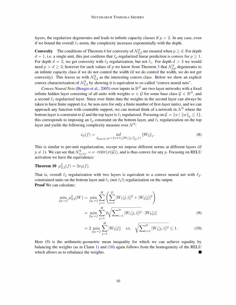
Theorem 10 µ22,2(f) = 2ν2(f).

That is, overall `2 regularization with two layers is equivalent to a convex neural net with `2-constrained units on the bottom layer and `1 (not `2!) regularization on the output.Proof We can calculate:

minfW=f

µ22,2(W ) = minfW=f

H∑j=1

(D∑i=1

|W1[j, i]|2 + |W2[j]|2)

= minfW=f

H∑j=1

2

√∑D

i=1|W1[j, i]|2 · |W2[j]| (9)

= 2 minfW=f

H∑j=1

|W2[j]| s.t.

√∑D

i=1|W1[j, i]|2 ≤ 1. (10)

Here (9) is the arithmetic-geometric mean inequality for which we can achieve equality bybalancing the weights (as in Claim 1) and (10) again follows from the homogeneity of the RELUwhich allows us to rebalance the weights.

10


Hardness As withN d1,∞, we might hope that the convexity ofN 2

2,2 might make it computationallyeasy to learn. However, by the same reduction from learning intersection of halfspaces (Theorem22 in Appendix E) we can again conclude that we cannot learn in time polynomial in µ22,2:

Corollary 11 Subject to the the strong random CSP assumptions in Daniely et al. (2014), it isnot possible to efficiently PAC learn (even improperly) functions ±1D → ±1 realizable with

unit margin by N 2p,p when µ2p,p = ω(D

1p ). (e.g. when γ1,∞ = D logD). Moreover, subject to in-

tractability of Q(D1.5)-unique shortest vector problem, for any ε > 0, it is not possible to efficientlyPAC learn (even improperly) functions ±1D → ±1 realizable with unit margin by N 2

1,∞ when

γ1,∞ = D1p+ε.

6. Depth Independent Regularization

Up until now we discussed relying on magnitude-based regularization instead of directly controllingnetwork size, thus allowing unbounded and even infinite width. But we still relied on a finite boundon the depth in all our derivations. Can the explicit dependence on the depth be avoided, andreplaced with only a measure of scale of the weights?

We already know we cannot rely only on a bound on the group-norm µp,q when the depth isunbounded, as we know from Theorem 3 that in terms of µp,q the sample complexity necessarilyincreases exponentially with the depth: if we allow arbitrarily deep graphs we can shrink µp,q towardzero without changing the scale of the computed function. However, controlling the γ-measure, orequivalently the path-regularizer φ, in arbitrarily-deep graphs is sensible, and we can define:

γp,q = infd≥1

γdp,q(f) = limd→∞

γdp,q(f) or: φp = infGφGp (f) (11)

where the minimization is over any DAG. From Theorem 6 we can conclude that φp(f) = γp,∞(f).In any case, γp,q(f) is a sensible complexity measure, that does not collapse despite the unboundeddepth. Can we obtain generalization guarantees for the class Nγp,q≤γ ?

Unfortunately, even when 1/p + 1/q ≥ 1 and we can obtain width-independent bounds, thebound in Corollary 2 still has a dependence on 4d, even if γp,q is bounded. Can such a dependencebe avoided?

For anti-symmetric Lipschitz-continuous activation functions (i.e. such that σ(−z) = −σ(z)),such as the ramp, and for per-unit `p-regularization µd1,∞ we can avoid the factor of 4d

Theorem 12 For any anti-symmetric 1-Lipschitz function σ and any set S = x1, . . . , xm ⊆ RD:

Rm(N d,σµ1,∞≤µ) ≤

√4µ2d log(2D) sup ‖xi‖2∞

m

The proof is again based on an inductive argument similar to Theorem 1 and you can find it inappendix A.4.

However, the ramp is not homogeneous and so the equivalent between µ, γ and φ breaks down.Can we obtain such a bound also for the RELU? At the very least, what we can say is that aninductive argument such that used in the proofs of Theorems 1 and 12 cannot be used to avoid an

11


exponential dependence on the depth. To see this, consider γ1,∞ ≤ 1 (this choice is arbitrary if weare considering the Rademacher complexity), for which we have

N d+1γ1,∞<1 =

[conv(N d

γ1,∞<1)]+, (12)

where conv(·) is the symmetric convex hull, and [·]+ = max(z, 0) is applied to each function inthe class. In order to apply the inductive argument without increasing the complexity exponentiallywith the depth, we would need the operation [conv(H)]+ to preserve the Rademacher complexity,at least for non-negative convex cones H. However we show a simple example of a non-negativeconvex coneH for whichRm ([conv(H)]+) > Rm (H).

We will specifyH as a set of vectors in Rm, corresponding to the evaluation of h(xi) of differentfunctions in the class on the m points xi in the sample. In our construction, we will have onlym = 3 points. Consider H = conv((1, 0, 1), (0, 1, 1)), in which case H′ , [conv(H)]+ =conv((1, 0, 1), (0, 1, 1), (0.5, 0, 0)). It is not hard to verify thatRm(H′) = 13

16 >1216 = Rm(H).

7. Summary and Open Issues

We presented a general framework for norm-based capacity control for feed-forward networks, andanalyzed when the norm-based control is sufficient and to what extent capacity still depends on otherparameters. In particular, we showed that in depth d > 2 networks, per-unit control with p > 1 andoverall regularization with p > 2 is not sufficient for capacity control without also controlling thenetwork size. This is in contrast with linear models, where with any p < ∞ we have only a weakdependence on dimensionality, and two-layer networks where per-unit p = 2 is also sufficient forcapacity control. We also obtained generalization guarantees for perhaps the most natural form ofregularization, namely `2 regularization, and showed that even with such control we still necessarilyhave an exponential dependence on the depth.

Although the additive µ-measure and multiplication γ-measure are equivalent at the optimum,they behave rather differently in terms of optimization dynamics (based on anecdotal empiricalexperience) and understanding the relationship between them, as well as the novel path-based reg-ularizer can be helpful in practical regularization of neural networks.

Although we obtained a tight characterization of when size-independent capacity control ispossible, the precise polynomial dependence of margin-based classification (and other tasks) on thenorm in might not be tight and can likely be improved, though this would require going beyondbounding the Rademacher complexity of the real-valued class. In particular, Theorem 1 gives thesame bound for per-unit `1 regularization and overall `1 regularization, although we would expectthe later to have lower capacity.

Beyond the open issue regarding depth-independent γ-based capacity control, another interest-ing open question is understanding the expressive power of N d

γp,q≤γ , particularly as a function ofthe depth d. Clearly going from depth d = 1 to depth d = 2 provides additional expressive power,but it is not clear how much additional depth helps. The class N 2 already includes all binary func-tions over ±1D and is dense among continuous real-valued functions. But can the γ-measure bereduced by increasing the depth? Viewed differently: γdp,q(f) is monotonically non-increasing ind, but are there functions for it continues decreasing? Although it seems obvious there are func-tions that require high depth for efficient representation, these questions are related to decade-oldproblems in circuit complexity and might not be easy to resolve.

12


Acknowledgments

This research was partially supported by NSF grant IIS-1302662 and an Intel ICRI-CI award. Wethank the COLT anonymous reviewers for pointing out an error in the statement of Lemma 15 andsuggesting other corrections.

References

Martin Anthony and Peter L. Bartlett. Neural network learning: Theoretical foundations. Cam-bridge University Press, 2009.

Francis Bach. Breaking the curse of dimensionality with convex neural networks. Technical report,HAL-01098505, 2014.

Maria-Florina Balcan and Christopher Berlind. A new perspective on learning linear separatorswith large lqlp margins. Proceedings of the Seventeenth International Conference on ArtificialIntelligence and Statistics, pages 68–76, 2014.

Peter L. Bartlett. The sample complexity of pattern classification with neural networks: the size ofthe weights is more important than the size of the network. IEEE transactions on informationtheory, 44(2):525–536, 1998.

Peter L. Bartlett and Shahar Mendelson. Rademacher and gaussian complexities: Risk bounds andstructural results. The Journal of Machine Learning Research, pages 463–482, 2003.

Yoshua Bengio, Nicolas L. Roux, Pascal Vincent, Olivier Delalleau, and Patrice Marcotte. Convexneural networks. Advances in neural information processing systems, pages 123–130, 2005.

Xavier Glorot Antoine Bordes and Yoshua Bengio. Deep sparse rectifier networks. AISTATS, 2011.

Youngmin Cho and Lawrence K. Saul. Kernel methods for deep learning. Advances in neuralinformation processing systems, pages 342–350, 2009.

Amit Daniely, Nati Linial, and Shai Shalev-Shwartz. From average case complexity to improperlearning complexity. STOC, 2014.

Uffe Haagerup. The best constants in the khintchine inequality. Studia Mathematica, 70(3):231–283, 1981.

Sham M Kakade, Karthik Sridharan, and AmbujTewari. On the complexity of linear prediction:Risk bounds, margin bounds, and regularization. Advances in neural information processingsystems, pages 793–800, 2009.

Adam R Klivans and Alexander A Sherstov. Cryptographic hardness for learning intersections ofhalfspaces. FOCS, pages 553–562, 2006.

Vladimir Koltchinskii and Dmitry Panchenko. Empirical margin distributions and bounding thegeneralization error of combined classifiers. Annals of Statistics, pages 1–50, 2002.

13


Wee Sun Lee, Peter L Bartlett, and Robert C Williamson. Efficient agnostic learning of neuralnetworks with bounded fan-in. Information Theory, IEEE Transactions on, 42(6):2118–2132,1996.

Roi Livni, Shai Shalev-Shwartz, and Ohad Shamir. On the computational efficiency of trainingneural networks. Advances in Neural Information Processing Systems, pages 855–863, 2014.

Vinod Nair and Geoffrey E. Hinton. Rectified linear units improve restricted boltzmann machines.ICML, 2010.

Shai Shalev-Shwartz and Shai Ben-David. Understanding Machine Learning: From Theory toAlgorithms. Cambridge University Press, 2014.

M.D. Zeiler, M. Ranzato, R. Monga, M. Mao, K. Yang, Q.V. Le, P. Nguyen, A. Senior, V. Van-houcke, J. Dean, and G.E. Hinton. On rectified linear units for speech processing. ICASSP,2013.

Appendix A. Rademacher Complexities

The sample based Rademacher complexity of a class F of function mapping from X to R withrespect to a set S = x1, . . . , xm is defined as:

Rm(F) = Eξ∈±1m

[1

msupf∈F

∣∣∣∣∣m∑i=1

ξif(xi)

∣∣∣∣∣]

In this section, we prove an upper bound for the Rademacher complexity of the classN d,H,σRELUγp,q≤γ ,

i.e., the class of functions that can be represented as depth d, width H network with rectified linearactivations, and the layer-wise group norm complexity γp,q bounded by γ. As mentioned in themain text, our proof is an induction with respect to the depth d. We start with d = 1 layer neuralnetworks, which is essentially the class of linear separators.

A.1. `p-regularized Linear Predictors

For completeness, we prove the upper bounds on the Rademacher complexity of class of linearseparators with bounded `p norm. The upper bounds presented here are particularly similar togeneralization bounds in Kakade et al. (2009) and Balcan and Berlind (2014). We first mention twoalready established lemmas that we use in the proofs.

Theorem 13 (Khintchine-Kahane Inequality) For any 0 < p < ∞ and S = z1, . . . , zm, if therandom variable ξ is uniform over ±1m, then(

Eξ

[∣∣∣∣∣m∑i=1

ξizi

∣∣∣∣∣p]) 1

p

≤ Cp

(m∑i=1

|zi|2) 1

2

where Cp is a constant depending only on p.

14


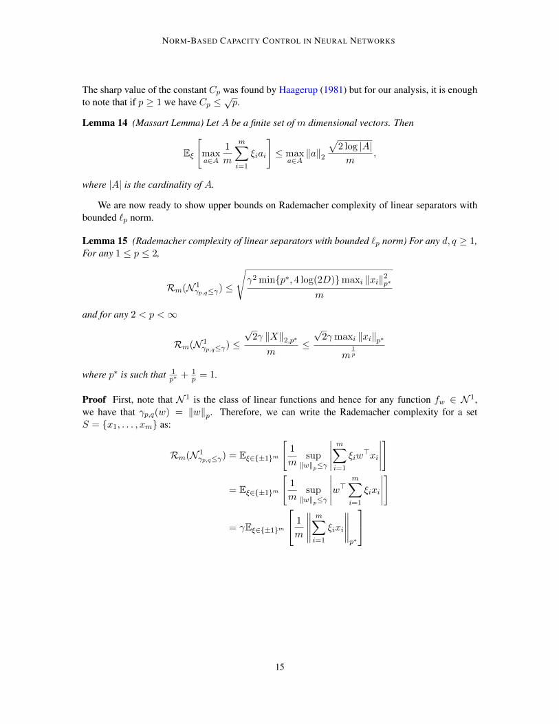
The sharp value of the constant Cp was found by Haagerup (1981) but for our analysis, it is enoughto note that if p ≥ 1 we have Cp ≤

√p.

Lemma 14 (Massart Lemma) Let A be a finite set of m dimensional vectors. Then

Eξ

[maxa∈A

1

m

m∑i=1

ξiai

]≤ max

a∈A‖a‖2

√2 log |A|m

,

where |A| is the cardinality of A.

We are now ready to show upper bounds on Rademacher complexity of linear separators withbounded `p norm.

Lemma 15 (Rademacher complexity of linear separators with bounded `p norm) For any d, q ≥ 1,For any 1 ≤ p ≤ 2,

Rm(N 1γp,q≤γ) ≤

√γ2 minp∗, 4 log(2D)maxi ‖xi‖2p∗

m

and for any 2 < p <∞


√2γ ‖X‖2,p∗

m≤√

2γmaxi ‖xi‖p∗

m1p

where p∗ is such that 1p∗ + 1

p = 1.

Proof First, note that N 1 is the class of linear functions and hence for any function fw ∈ N 1,we have that γp,q(w) = ‖w‖p. Therefore, we can write the Rademacher complexity for a setS = x1, . . . , xm as:

Rm(N 1γp,q≤γ) = Eξ∈±1m

[1

msup‖w‖p≤γ

∣∣∣∣∣m∑i=1

ξiw>xi

∣∣∣∣∣]

= Eξ∈±1m

[1

msup‖w‖p≤γ

∣∣∣∣∣w>m∑i=1

ξixi

∣∣∣∣∣]

= γEξ∈±1m

1

m

∥∥∥∥∥m∑i=1

ξixi

∥∥∥∥∥p∗

15


For 1 ≤ p ≤ min

2, 2 log(2D)2 log(2D)−1

(and therefore 2 log(2D) ≤ p∗), we have

Rm(N 1γp,q≤γ) = γEξ∈±1m

1

m

∥∥∥∥∥m∑i=1

ξixi

∥∥∥∥∥p∗

≤ D

1p∗ γEξ∈±1m

[1

m

∥∥∥∥∥m∑i=1

ξixi

∥∥∥∥∥∞

]

≤ D1

2 log(2D)γEξ∈±1m

[1

m

∥∥∥∥∥m∑i=1

ξixi

∥∥∥∥∥∞

]

≤√

2γEξ∈±1m

[1

m

∥∥∥∥∥m∑i=1

ξixi

∥∥∥∥∥∞

]

We now use the Massart Lemma viewing each feature (xi[j])mi=1 for j = 1, . . . , D as a member of

a finite hypothesis class and obtain


√2γEξ∈±1m

[1

m

∥∥∥∥∥m∑i=1

ξixi

∥∥∥∥∥∞

]

≤ 2γ

√log(2D)

mmaxj=1...,D

‖(xi[j])mi=1‖2

≤ 2γ

√log(2D)

mmax

i=1,...,m‖xi‖∞

≤ 2γ

√log(2D)

mmax

i=1,...,m‖xi‖p∗

If min

2, 2 log(2D)2 log(2D)−1

< p <∞, by Khintchine-Kahane inequality we have

Rm(N 1γp,q≤γ) = γEξ∈±1m

1

m

∥∥∥∥∥m∑i=1

ξixi

∥∥∥∥∥p∗

≤ γ 1

m

D∑j=1

Eξ∈±1m

∣∣∣∣∣m∑i=1

ξixi[j]

∣∣∣∣∣p∗1/p∗

≤ γ√p∗

m

(∑D

j=1‖(xi[j])mi=1‖

p∗

2

)1/p∗

= γ

√p∗

m‖X‖2,p∗

If p∗ ≥ 2, by Minskowski inequality we have that ‖X‖2,p∗ ≤ m1/2 maxi ‖xi‖p∗ . Otherwise, by

subadditivity of the function f(z) = zp∗2 , we get ‖X‖2,p∗ ≤ m1/p∗ maxi ‖xi‖p∗ .

16


A.2. Theorem 1

We define the hypothesis class N d,H,H to be the class of functions from X to RH computed by alayered network of depth d, layer size H and H outputs.

For the proof of theorem 1, we need the following two technical lemmas. The first is the well-known contraction lemma:

Lemma 16 (Contraction Lemma) Let function φ : R → R be Lipschitz with constant Lφ suchthat φ satisfies φ(0) = 0. Then for any class F of functions mapping from X to R and any setS = x1, . . . , xm:

Eξ∈±1m

[1

msupf∈F

∣∣∣∣∣m∑i=1

ξiφ(f(xi))

∣∣∣∣∣]≤ 2LφEξ∈±1m

[1

msupf∈F

∣∣∣∣∣m∑i=1

ξif(xi))

∣∣∣∣∣]

Next, the following lemma reduces the maximization over a matrix W ∈ RH×H that appears in thecomputation of Rademacher complexity to H independent maximizations over a vector w ∈ RH(the proof is deferred to Subsection A.3):

Lemma 17 For any p, q ≥ 1, d ≥ 2, ξ ∈ ±1m and f ∈ N d,H,H we have

supW

1

‖W‖p,q

∥∥∥∥∥m∑i=1

ξi[W [f(xi)]+]+

∥∥∥∥∥p∗

= H[ 1p∗−

1q]+ sup

w

1

‖w‖p

∣∣∣∣∣m∑i=1

ξi[w>[f(xi)]+]+

∣∣∣∣∣where p∗ is such that 1

p∗ + 1p = 1.

Theorem 1 For any d, p, q ≥ 1 and any set S = x1, . . . , xm ⊆ RD:

Rm(N d,H,σRELU

γp,q≤γ ) ≤

√√√√γ2(

2H[ 1p∗−

1q]+)2(d−1)

minp∗, 2 log(2D) sup ‖xi‖2p∗m

and so:

Rm(N d,H,σRELU

µp,q≤µ ) ≤

√√√√µ2d(

2H[ 1p∗−

1q]+/ q√d)2(d−1)

minp∗, 2 log(2D) sup ‖xi‖2p∗m

where p∗ is such that 1p∗ + 1

p = 1.

17


Proof By the definition of Rademacher complexity if ξ is uniform over ±1m, we have:

Rm(N d,Hγp,q≤γ) = Eξ

1

msup

f∈N d,Hγp,q≤γ

∣∣∣∣∣m∑i=1

ξif(xi)

∣∣∣∣∣

= Eξ

[1

msup

f∈N d,H

γ

γp,q(f)

∣∣∣∣∣m∑i=1

ξif(xi)

∣∣∣∣∣]

= Eξ

[1

msup

g∈N d−1,H,H

supw

γ

γp,q(g) ‖w‖p

∣∣∣∣∣m∑i=1

ξiw>[g(xi)]+

∣∣∣∣∣]

= Eξ

1

msup

g∈N d−1,H,H

γ

γp,q(g)

∥∥∥∥∥m∑i=1

ξi[g(xi)]+

∥∥∥∥∥p∗

= Eξ

1

msup

h∈N d−2,H,H

γ

γp,q(h)supW

1

‖W‖p,q

∥∥∥∥∥m∑i=1

ξi[W [h(xi)]+]+

∥∥∥∥∥p∗

= H

[ 1p∗−

1q]+Eξ

[1

msup

h∈N d−2,H,H

γ

γp,q(h)supw

1

‖w‖p

∣∣∣∣∣m∑i=1

ξi[w>[h(xi)]+]+

∣∣∣∣∣]

(13)

= H[ 1p∗−

1q]+Eξ

1

msup

g∈N d−1,Hγp,q≤γ

∣∣∣∣∣m∑i=1

ξi[g(xi)]+

∣∣∣∣∣

≤ 2H[ 1p∗−

1q]+Eξ

1

msup

g∈N d−1,Hγp,q≤γ

∣∣∣∣∣m∑i=1

ξig(xi)

∣∣∣∣∣ (14)

= 2H[ 1p∗−

1q]+Rm(N d−1,H

γp,q≤γ )

where the equality (13) is obtained by lemma 17 and inequality (14) is by Contraction Lemma.This will give us the bound on Rademacher complexity of N d,H

γp,q≤γ based on the Rademacher

complexity of N d−1,Hγp,q≤γ . Applying the same argument on all layers and using lemma 15 to bound

the complexity of the first layer completes the proof.

A.3. Proof of Lemma 17

Proof It is immediate that the right hand side of the equality in the statement is always less thanor equal to the left hand side because given any vector w in the right hand side, by setting eachrow of matrix W in the left hand side we get the equality. Therefore, it is enough to prove thatthe left hand side is less than or equal to the right hand side. For the convenience of notations, letg(w) , |

∑mi=1 ξiw

>[f(xi)]+|. Define w to be:

w , arg maxw

g(w)

‖w‖p

18


If q ≤ p∗, then the right hand side of equality in the lemma statement will reduce to g(w)/ ‖w‖pand therefore we need to show that for any matrix V ,

g(w)

‖w‖p≥‖g(V )‖p∗‖V ‖p,q

.

Since q ≤ p∗, we have ‖V ‖p,p∗ ≤ ‖V ‖p,q and hence it is enough to prove the following inequality:

g(w)

‖w‖p≥‖g(V )‖p∗‖V ‖p,p∗

.

On the other hand, if q > p∗, then we need to prove the following inequality holds:

H1p∗−

1qg(w)

‖w‖p≥‖g(V )‖p∗‖V ‖p,q

Since q > p∗, we have that ‖V ‖p,p∗ ≤ H1p∗−

1q ‖V ‖p,q. Therefore, it is again enough to show that:

g(w)

‖w‖p≥‖g(V )‖p∗‖V ‖p,p∗

.

We can rewrite the above inequality in the following form:

H∑i=1

(g(w) ‖Vi‖p‖w‖p

)p∗≥

H∑i=1

g(Vi)p∗

By the definition of w, we know that the above inequality holds for each term in the sum and hencethe inequality is true.

A.4. Theorem 12

The proof is similar to the proof of theorem 1 but here bounding µ1,∞ by µ means the `1 norm ofinput weights to each neuron is bounded by µ. We use a different version of Contraction Lemma inthe proof that is without the absolute value:

Lemma 18 (Contraction Lemma (without the absolute value)) Let function φ : R→ R be Lipschitzwith constant Lφ. Then for any class F of functions mapping from X to R and any set S =x1, . . . , xm:

Eξ∈±1m

[1

msupf∈F

m∑i=1

ξiφ(f(xi))

]≤ LφEξ∈±1m

[1

msupf∈F

m∑i=1

ξif(xi))

]

Theorem 12 For any anti-symmetric 1-Lipschitz function σ and any set S = x1, . . . , xm ⊆ RD:

Rm(N d,σµ1,∞≤µ) ≤

√2µ2d log(2D) sup ‖xi‖2∞

m

19


Proof Assuming ξ is uniform over ±1m, we have:

Rm(N d,Hµ1,∞≤µ) = Eξ

1

msup

f∈N d,Hµ1,∞≤µ

∣∣∣∣∣m∑i=1

ξif(xi)

∣∣∣∣∣

= Eξ

1

msup

f∈N d,Hµ1,∞≤µ

m∑i=1

ξif(xi)

= Eξ

1

msup

g∈N d−1,H,Hµ1,∞≤µ

sup‖w‖1≤µ

w>m∑i=1

ξiσ(g(xi))

= Eξ

1

msup

g∈N d−1,H,Hµ1,∞≤µ

∥∥∥∥∥m∑i=1

ξiσ(g(xi))

∥∥∥∥∥∞

= Eξ

1

msup

g∈N d−1,Hµ1,∞≤µ

∣∣∣∣∣m∑i=1

ξiσ(g(xi))

∣∣∣∣∣ (15)

= Eξ

1

msup


m∑i=1

ξiσ(g(xi))

≤ Eξ

1

msup


m∑i=1

ξig(xi)

(16)

= Eξ

1

msup


∣∣∣∣∣m∑i=1

ξig(xi)

∣∣∣∣∣

= Rm(N d−1,Hµ1,∞≤µ)

where the equality (15) is by anti-symmetric property of σ and inequality (16) is by the versionof Contraction Lemma without the absolute value. This will give us the bound on Rademachercomplexity of N d,H

µ1,∞≤µ based on the Rademacher complexity of N d−1,Hµ1,∞≤µ. Applying the same

argument on all layers and using lemma 15 to bound the complexity of the first layer completes theproof.

Appendix B. Tightness

We repeat the theorem statement here for convenience.

Theorem 3 For any p, q ≥ 1 (and 1/p∗ + 1/p = 1) and any depth d ≥ 2, the m = 2D points±1D can be shattered with unit margin by N d,H

γp,q≤γ with:

γ ≤ D1/pm1/p+1/qH−(d−2)[1/p∗−1/q]+ .

20


Proof Consider a size m subset Sm of 2D vertices of the D dimensional hypercube −1,+1D.We construct the first layer using m units. Each unit has a unique weight vector consisting of +1and−1’s and will output a positive value if and only if the sign pattern of the input x ∈ Sm matchesthat of the weight vector. The second layer has a single unit and connects to all m units in thefirst layer. For any m dimensional sign pattern b ∈ −1,+1m, we can choose the weights of thesecond layer to be b, and the network will output the desired sign for each x ∈ Sm with unit margin.The norm of the network is at most (m ·Dq/p)1/q ·m1/p = D1/p ·m(1/p+1/q). This establishes theclaim for d = 2. For d > 2 and 1/p+ 1/q ≥ 1, we obtain the same norm and unit margin by addingd− 2 layers with one unit in each layer connected to the previous layer by a unit weight. For d > 2and 1/p + 1/q < 1, we show the dependence on H by recursively replacing the top unit with Hcopies of it and adding an averaging unit on top of that. More specifically, given the above d = 2layer network, we make H copies of the output unit with rectified linear activation and add a 3rdlayer with one output unit with uniform weight 1/H to all the copies in the 2nd layer. Since thisoperation does not change the output of the network, we have the same margin and now the norm ofthe network is (m ·Dq/p)1/q · (Hmq/p)1/q · (H(1/Hp))1/p = D1/p ·m(1/p+1/q) ·H1/q−1/p∗ . Thatis, we have reduced the norm by factor H1/q−1/p∗ . By repeating this process, we get the geometricreduction in the norm H(d−2)(1/q−1/p∗), which concludes the proof.

Appendix C. Proof that γdp,q(f) is a semi-norm in N d

Theorem 4 For any d, p, q ≥ 1 such that 1q ≤

1d−1(1− 1

p

), γdp,q(f) is a semi-norm in N d.

Proof The proof consists of three parts. First we show that the level set N dγdp,q≤γ

= f ∈ N d :

γdp,q(f) ≤ γ is a convex set if the condition on d, p, q is satisfied. Next, we establish the non-negative homogeneity of γdp,q(f). Finally, we show that if a function α : N d → R is non-negativehomogeneous and every sublevel set f ∈ N d : α(f) ≤ γ is convex, then α satisfies the triangularinequality.

Convexity of the level sets First we show that for any two functions f1, f2 ∈ N dγp,q≤γ and 0 ≤

α ≤ 1, the function g = αf1 + (1 − α)f2 is in the hypothesis class N dγp,q≤γ . We prove this by

constructing weights W that realizes g. Let U and V be the weights of two neural networks suchthat γp,q(U) = γdp,q(f1) ≤ γ and γp,q(V ) = γdp,q(f2) ≤ γ. For every layer i = 1, . . . , d let

Ui = d

√γp,q(U)Ui/‖Ui‖p,q, Vi = d

√γp,q(V )Vi/‖Vi‖p,q.

and set W1 =

[U1

V1

]for the first layer, Wi =

[Ui 0

0 Vi

]for the intermediate layers and Wd =[

αUd (1− α)Vd]

for the output layer.Then for the defined W , we have fW = αf1 + (1 − α)f2 for rectified linear and any other

non-negative homogeneous activation function. Moreover, for any i < d, the norm of each layer is

‖Wi‖p,q =(γp,q(U)

qd + γp,q(V )

qd

) 1q ≤ 2

1q γ

1d (17)

21


and in layer d we have:

‖Wd‖p =(αpγp,q(U)

pd + (1− α)pγp,q(V )

pd

) 1p ≤ 21/p−1γ1/d (18)

Combining inequalities (17) and (18), we get γdp,q(fW ) ≤ 2d−1q

+ 1pγ ≤ γ, where the last inequality

holds because we assume that 1q ≤

1d−1(1− 1

p

). Thus for every γ ≥ 0, N d

γp,q≤γ is a convex set.

Non-negative homogeneity For any function f ∈ N d and any α ≥ 0, let U be the weightsrealizing f with γdp,q(f) = γp,q(U). Then d

√αU realizes αf establishing γdp,q(αf) ≤ γp,q( d

√αU) =

αγp,q(U) = αγdp,q(U) = αγdp,q(f). This establishes the non-negative homogeneity of γdp,q.

Convex sublevel sets and homogeneity imply triangular inequality Let α(f) be non-negativehomogeneous and assume that every sublevel set f ∈ N d : α(f) ≤ γ is convex. Then forf1, f2 ∈ N d, defining γ1 , α(f1), γ2 , α(f2), f1 , (γ1 + γ2)f1/γ1, and f2 , (γ1 + γ2)f2/γ2,we have

α(f1 + f2) = α

(γ1

γ1 + γ2f1 +

γ2γ1 + γ2

f2

)≤ γ1 + γ2 = α(f1) + α(f2).

Here the inequality is due to the convexity of the level set and the fact that α(f1) = α(f2) = γ1+γ2,because of the homogeneity. Therefore α satisfies the triangular inequality and thus it is a seminorm.

Appendix D. Path Regularization

D.1. Theorem 5

Lemma 19 For any function f ∈ N d,Hγp,∞≤γ there is a layered network with weights w such that

γp,∞(w) = γd,Hp,∞(f) and for any internal unit v,∑

(u→v)∈E |w(u→ v)|p = 1.

Proof Let w be the weights of a network such that γp,∞(w) = γd,Hp,∞(f). We now construct a net-work with weights w such that γp,∞(w) = γd,Hp,∞(f) and for any internal unit v,

∑(u→v)∈E |w(u→

v)|p = 1. We do this by an incremental algorithm. Let w0 = w. At each step i, we do the following.Consider the first layer, Set Vk to be the set of neurons in the layer k. Let x be the maximum of

`p norms of input weights to each neuron in set V1 and let Ux ⊆ V1 be the set of neurons whose `pnorms of their input weight is exactly x. Now let y be the maximum of `p norms of input weightsto each neuron in the set V1 \ Ux and let Uy be the set of the neurons such that the `p norms oftheir input weights is exactly y. Clearly y < x. We now scale down the input weights of neuronsin set Ux by y/x and scale up all the outgoing edges of vertices in Ux by x/y (y cannot be zerofor internal neurons based on the definition). It is straightforward that the new network realizes thesame function and the `p,∞ norm of the first layer has changed by a factor y/x. Now for everyneuron v ∈ V2, let r(v) be the `p norm of the new incoming weights divided by `p norm of theoriginal incoming weights. We know that r(v) ≤ x/y. We again scaly down the input weights ofeveryv ∈ V2 by 1/r(v) and scale up all the outgoing edges of v by r(v). Continuing this operationto on each layer, each time we propagate the ratio to the next layer while the network always realizes

22


the same function and for each layer k, we know that for every v ∈ Vk, r(v) ≤ x/y. After thisoperation, in the network, the `p,∞ norm of the first layer is scaled down by y/x while the `p,∞norm of the last layer is scaled up by at most x/y and the `p,∞ norm of the rest of the layers hasremained the same. Therefore, if wi is the new weight setting, we have γp,∞(wi) ≤ γp,∞(wi−1).

After continuing the above step at most |V1| − 1 times, the `p norm of input weights is the samefor all neurons in V1. We can then run the same algorithm on other layers and at the end we havea network with weight setting w such that the for each k < d, `p norm of input weight to each ofthe neurons in layer k is equal to each other and γp,∞(w) ≤ γp,∞(w). This is in fact an equalitybecause weight setting w′ realizes function f and we know that γp,∞(w) = γd,Hp,∞(f). A simplescaling of weights in layers gives completes the proof.

Theorem 5 For p ≥ 1, any d and (finite or infinite) H , for any f ∈ N d,H : φd,Hp (f) = γd,Hp,∞.

Proof By the Lemma 19, there is a layered network with weights w such that γp,∞(w) = γd,Hp,∞(f)and for any internal unit v,

∑(u→v)∈E |w(u → v)|p = 1. Let W be the weights of the layered

network that corresponds to the function w. Then we have:

vp(w) =

∑vin[i]

e1→v1e2→v2···

ek→vout

k∏i=1

|w(ei)|p

1p

(19)

=

H∑id−1=1

· · ·H∑i1=1

D∑i0=1

|Wd[id−1]|pd−1∏k=1

|Wk[ik, ik−1]|p 1

p

(20)

=

H∑id−1=1

|Wd[id−1]|p · · ·H∑i1=1

|Wk[i2, i1]|pD∑i0=1

|Wk[i1, i0]|p 1

p

(21)

=

H∑id−1=1

|Wd[id−1]|p · · ·H∑i1=1

|Wk[i2, i1]|p 1

p

(22)

=

H∑id−1=1

|Wd[id−1]|p · · ·H∑i2=1

|Wk[i3, i2]|p 1

p

(23)

=

H∑id−1=1

|Wd[id−1]|p 1

p

= `p(Wd) = γp,∞(W ) (24)

(25)

where inequalities 20 to 24 are due to the fact that the `p norm of input weights to each internalneuron is exactly 1 and the last equality is again because `p,∞ of all layers is exactly 1 except thelayer d.

23


D.2. Proof of Theorem 6

In this section, without loss of generality, we assume that all the internal nodes in a DAG haveincoming edges and outgoing edges because otherwise we can just discard them. Let dout(v) be thelongest directed path from vertex v to vout and din(v) be the longest directed path from any inputvertex vin[i] to v. We say graph G is a sublayered graph if G is a subgraph of a layered graph.

We first show the necessary and sufficient conditions under which a DAG is a sublayered graph.

Lemma 20 The graph G(E, V ) is a sublayered graph if and only if any path from input nodes tothe output nodes has length d where d is the length of the longest path in G

Proof Since the internal nodes have incoming edges and outgoing edges; hence ifG is a sublayeredgraph it is straightforward by induction on the layers that for every vertex v in layer i, there is avertex u in layer i + 1 such that (v → u) ∈ E and this proves the necessary condition for beingsublayered graph.

To show the sufficient condition, for any internal node u, u has din(v) distance from the inputnode in every path that includes u (otherwise we can build a path that is longer than d). Therefore,for each vertex v ∈ V , we can place vertex v in layer din(v) and all the outgoing edges from v willbe to layer din(v) + 1.

Lemma 21 If the graph G(E, V ) is not a sublayered graph then there exists a directed edge (u→v) such that din(u) + dout(v) < d− 1 where d the length of the longest path in G.

Proof We prove the lemma by an inductive argument. If G is not sublayered, by lemma 20, weknow that there exists a path v0 → . . . vi · · · → vd′ where v0 is an input node (din(v0) = 0),vd′ = vout (dout(vd′ = 0) and d′ < d. Now consider the vertex v1. We need to have dout(v1) = d−1otherwise if dout(v1) < d− 1 we get din(u) + dout(v) < d− 1 and if dout(v1) > d− 1 there will bepath in G that is longer than d. Also, since dout(v1) = d− 1 and the longest path in G has length d,we have din(v1) = 1.

By applying the same inductive argument on each vertex vi in the path we get din(vi) = i anddout(vi) = d − i. Note that if the condition din(u) + dout(v) < d − 1 is not satisfied in one of thesteps of the inductive argument, the lemma is proved. Otherwise, we have din(vd′−1) = d′ − 1 anddout(vd′−1) = d − d′ + 1 and therefore din(vd′−1) + dout(vout) = d′ − 1 < d − 1 that proves thelemma.

Theorem 6 For any p ≥ 1 and any d: γdp,∞(f) = minG ∈ DAG(d)

φGp (f).

Proof Consider any fG,w ∈ NDAG(d) where the graphG(E, V ) is not sublayered. Let ρ be the totalnumber of paths from input nodes to the output nodes. Let T be sum over paths of the length of thepath. We indicate an algorithm to change G into a sublayered graph G of depth d with weights wsuch that fG,w = fG,w and φ(w) = φ(w). Let G0 = G and w0 = w.

At each step i, we consider the graph Gi−1. If Gi−1 is sublayered, we are done otherwise bylemma 21, there exists an edge (u→ v) such that din(u)+dout(v) < d−1. Now we add a new vertexvi to graph Gi−1, remove the edge (u → v), add two edges (u → vi) and (vi → v) and return the

24


graph asGi and since we had din(u)+dout(v) < d−1 inGi−1, the longest path inGi still has lengthd. We also set w(u → vi) =

√|w(u→ v)| and w(vi → v) = sign(w(u → v))

√|w(u→ v)|.

Since we are using rectified linear units activations, for any x > 0, we have [x]+ = x and therefore:

w(vi → v) [w(u→ vi)o(u)]+ = sign(w(u→ v))√|w(u→ v)|

[√|w(u→ v)|o(u)

]+

= sign(w(u→ v))√|w(u→ v)|

√|w(u→ v)|o(u)

= w(u→ v)o(u)

So we conclude that fGi,wi = fGi−1,wi−1 . Clearly, since we didn’t change the length of any pathfrom input vertices to the output vertex, we have φ(w) = φ(w). Let Ti be sum over paths of thelength of the path in Gi. It is clear that Ti−1 ≤ Ti because we add a new edge into a path at eachstep. We also know by lemma 20 that if Ti = ρd, then Gi is a sublayered graph. Therefore, afterat most ρd − T0 steps, we return a sublayered graph G and weights w such that fG,w = fG,w. Wecan easily turn the sublayered graph G a layered graph by adding edges with zero weights and thistogether with Theorem 5 completes the proof.

D.3. Proof of Theorem 9

Theorem 9 For any p ≥ 1 and d > 1 and any f ∈ N d, there exists a layered graph G(V,E) ofdepth d, such that f ∈ NG and γGp,∞(f) = φGp (f) = γdp,∞(f), and the out-degree of every internal(non-input) node in G is one. That is, the subgraph of G induced by the non-input vertices is a treedirected toward the output vertex.

Proof For any fG,w ∈ NDAG(d), we show how to construct such G and w. We first sort the verticesof G based on topological ordering such that the out-degree of the first vertex is zero. Let G0 = Gand w0 = w. At each step i, we first set Gi = Gi−1 and wi = wi−1 and then pick the vertex u thatis the ith vector in the topological ordering. If the out-degree of u is at most 1. Otherwise, for anyedge (u → v) we create a copy of vertex u that we call it uv, add the edge (uv → v) to Gi andconnect all incoming edges of u with the same weights to every such uv and finally we delete thevertex u from Gi together with all incoming and outgoing edges of u. It is easy to indicate thatfGi,wi = fGi−1,wi−1 . After at most |V | such steps, all internal nodes have out-degree one and hencethe subgraph induced by non-input vertices will be a tree.

Appendix E. Hardness of Learning Neural Networks

Daniely et al. (2014) show in Theorem 5.4 and in Section 7.2 that subject to the strong random CSPassumption, for any k = ω(1) the hypothesis class of intersection of homogeneous halfspaces over±1n with normals in ±1 is not efficiently PAC learnable (even improperly)2. Furthermore,for any ε > 0, Klivans and Sherstov (2006) prove this hardness result subject to intractability ofQ(D1.5)-unique shortest vector problem for k = Dε.

2. Their Theorem 5.4 talks about unrestricted halfspaces, but the construction in Section 7.2 uses only data in ±1Dand halfspaces specified by 〈w, x〉 > 0 with w ∈ ±1D

25


If it is not possible to efficiently PAC learn intersection of halfspaces (even improperly), we canconclude it is also not possible to efficiently PAC learn any hypothesis class which can representsuch intersection. In Theorem 22 we show that intersection of homogeneous half spaces can berealized with unit margin by neural networks with bound norm.

Theorem 22 For any k > 0, the intersection of k homogeneous half spaces is realizable with unitmargin by N 2

γp,q≤γ where γ = 4D1pk2.

Proof The proof is by a construction that is similar to the one in Livni et al. (2014). For eachhyperplane 〈wi, x〉 > 0, where wi ∈ ±1D, we include two units in the first layer: g+i (x) =[〈wi, x〉]+ and g−i (x) = [〈wi, x〉 − 1]+. We set all incoming weights of the output node to be 1.Therefore, this network is realizing the following function:

f(x) =

k∑i=1

([〈wi, x〉]+ − [〈wi, x〉 − 1]+)

Since all inputs and all weights are integer, the outputs of the first layer will be integer,([〈wi, x〉]+ − [〈wi, x〉 − 1]+) will be zero or one, and f realizes the intersection of the k halfspaceswith unit margin. Now, we just need to make sure that γ2p,q(f) is bounded by γ = 4D

1pk2:

γ2p,q(f) = D1p (2k)

1q (2k)

1p

≤ D1p (2k)2 = γ.

26

norm-based capacity control in neural networksproceedings.mlr.press/v40/neyshabur15.pdf ·...

Documents