IFAC Journal of Systems and Control 6 (2018) 33–42

Contents lists available at ScienceDirect

IFAC Journal of Systems and Control

journal homepage: www.elsevier.com/locate/ifacsc

Nonstandard use of anti-windup loop for systems with input backlashSophie Tarbouriech a,∗, Isabelle Queinnec a, Christophe Prieur b

a LAAS-CNRS, Université de Toulouse, CNRS, Toulouse, Franceb Univ. Grenoble Alpes, CNRS, Grenoble-INP, GIPSA-lab, F-38000, Grenoble, France

a r t i c l e i n f o

Article history:Received 13 July 2018Accepted 18 October 2018Available online xxxx

Keywords:Stability analysisStabilizationBacklashAnti-windup loops

a b s t r a c t

Control systems with backlash at the input are considered in this paper. The goal of this work is tocharacterize the attractor of such nonlinear dynamical systems, and to design anti-windup inspired loopssuch that the system is globally asymptotically stablewith respect to this attractor. The anti-windup loopsaffect the dynamics of the controllers, and allow to increase the performance of the closed-loop systems.Different performance issues are considered throughout the paper such as robustness with respect touncertainty in the backlash, and L2 gain when external disturbances affect the dynamics. Numericallytractable algorithms with feasibility guarantee are provided, as soon as the linear closed-loop system,obtained by neglecting the backlash effect, is asymptotically stable. The results are illustrated on anacademic example and an open-loop unstable aircraft system.

© 2018 Elsevier Ltd. All rights reserved.

1. Introduction

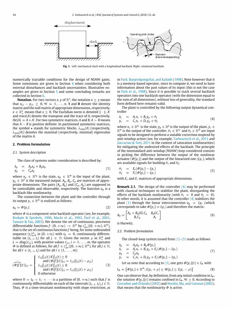
Backlash operators are nonlinearities present in manymechan-ical systems. They are involved inmechanical slacks, static friction,elastic displacements and ferromagnetism. Fig. 1 shows some ex-amples andMacki, Nistri, and Zecca (1993) is a good introduction ofthis kind of nonlinearity. Sincemany smart actuators andmaterialscontain a backlash, and since they are often used for precise controlsystems, such as position regulation, it is crucial to take the back-lash operator into account in the design or the analysis of the closedloop. Neglecting them can reduce the performance or alleviate thestability objective.

There are many different models for backlash operators, seeMacki et al. (1993) for a survey of possible models. Here we willfocus on a component-wise model considered in Brokate andSprekels (1996), Macki et al. (1993), Ouyang and Jayawardhana(2014), Paré, Hassibi, and How (2001) and Taware and Tao (2003).The undesirable effect of such a nonlinearity map has been alreadyanalyzed using circle criterion in Jayawardhana, Logemann, andRyan (2011), assuming that the control system is open-loop stable,an assumption that is not required in this paper. The presentwork is based on a Lyapunov method for control systems withbacklash operators in the loop. The control objective is to reducethe undesirable effect of the nonlinearity by adding an extra dy-namics. Such a strategy inspired by anti-windup techniques hasbeen already employed for control systems with saturated inputs,see e.g. Tarbouriech, Garcia, Gomes da Silva, and Queinnec (2011)

∗ Corresponding author.E-mail addresses: tarbour@laas.fr (S. Tarbouriech), queinnec@laas.fr

(I. Queinnec), christophe.prieur@gipsa-lab.fr (C. Prieur).

and Zaccarian and Teel (2011), where it is shown how to design socalled anti-windup gains to improve the performance of saturatingclosed-loop systems.

To be more specific, our contribution is as follows. We succeedto compute numerically tractable conditions for the design ofnonstandard anti-windup (NSAW) gains thatmodify the controllerdynamics and its output for different control objectives. In pres-ence of backlash operators, the most natural control objective isprobably the reduction of the attractor that is the reduction of theultimate bounded set where all solutions converge. In an ideal casewhere the backslash is not present, the attractor is usually reducedto one point, thus our NSAW technique can be seen as a method toapproach as much as possible the ideal case.

Another natural control objective is the robustness issue, that isto guarantee some stability properties in presence of external per-turbations or disturbances in the loop and in the backlash operator.The Lyapunov method applies for such cases, and we show how todesign NSAW gains guaranteeing the best performance in terms ofrobustness, with respect to uncertainty in the backlash and withrespect to external disturbances. Again our design conditions arenumerically tractable and apply as soon as the closed-loop system,without any backlash, is asymptotically stable. On the other hand,no restrictive hypothesis is necessary regarding the open-loopstability of the system. More precisely, our conditions are based onthe solution to a convex problemwritten in terms of Linear MatrixInequalities that are shown to have a solution allowing to explicitlycompute NSAW gains.

The paper is organized as follows. The stability problem andthe NSAW gain design problem are introduced in Section 2 forbacklash control systems. The main results are given in Section 3yielding a solution to the stability analysis and allowing to compute

https://doi.org/10.1016/j.ifacsc.2018.10.0032468-6018/© 2018 Elsevier Ltd. All rights reserved.

34 S. Tarbouriech et al. / IFAC Journal of Systems and Control 6 (2018) 33–42

Fig. 1. Left: mechanical slack with a longitudinal backlash. Right: rotational backlash.

numerically tractable conditions for the design of NSAW gains.Some extensions are given in Section 4 when considering bothexternal disturbances and backlash uncertainties. Illustrative ex-amples are given in Section 5 and some concluding remarks arecollected in Section 6.

Notation. For two vectors x, y of Rn, the notation x ⪰ y meansthat x(i) − y(i) ≥ 0, ∀i = 1, . . . , n. 1 and 0 denote the identitymatrix and the nullmatrix of appropriate dimensions, respectively.x ∈ Rn

+means that x ⪰ 0. The Euclidian norm is denoted ∥ · ∥. A′

and trace(A) denote the transpose and the trace of A, respectively.He{A} = A+A′. For two symmetric matrices, A and B, A > Bmeansthat A − B is positive definite. In partitioned symmetric matrices,the symbol ⋆ stands for symmetric blocks. λmax(A) (respectively,λmin(A)) denotes the maximal (respectively, minimal) eigenvalueof the matrix A.

2. Problem formulation

2.1. System description

The class of systems under consideration is described by:

xp = Apxp + Bpupyp = Cpxp

(1)

where xp ∈ Rnp is the state, up ∈ Rm is the input of the plant,yp ∈ Rp is the measured output. Ap, Bp, Cp are matrices of appro-priate dimensions. The pairs (Ap, Bp) and (Cp, Ap) are supposed tobe controllable and observable, respectively. The function up is abacklash-like nonlinearity.

The connection between the plant and the controller throughits output yc ∈ Rm is realized as follows:

up = Φ[yc] (2)

whereΦ is a component-wise backlash operator (see, for example,Brokate & Sprekels, 1996, Macki et al., 1993, Paré et al., 2001,Taware & Tao, 2003). We denote the set of continuous, piecewisedifferentiable functions f : [0, +∞) → Rm by C1

pw([0, +∞);Rm),that is the set of continuous functions f being, for some unboundedsequence (tj)∞j=0 in [0, +∞) with t0 = 0, continuously differen-tiable on (tj−1, tj) for all j ∈ N. Given the vector ρ in Rm

+and

L = diag(ℓ(i)), with positive values ℓ(i), i = 1, . . . ,m, the operatorΦ is defined as follows, for all f ∈ C1

pw([0, +∞);Rm), for all j ∈ N,for all t ∈ (tj−1, tj) and for all i ∈ {1, . . . ,m}:

(˙

Φ[f ](t))(i) =

⎧⎪⎪⎪⎨⎪⎪⎪⎩ℓ(i) f(i)(t) if f(i)(t) ≥ 0

and (Φ[f ](t))(i) = ℓ(i)(f(i)(t) − ρ(i))ℓ(i) f(i)(t) if f(i)(t) ≤ 0

and (Φ[f ](t))(i) = ℓ(i)(f(i)(t) + ρ(i))0 otherwise

(3)

where 0 = t0 < t1 < · · · is a partition of [0, +∞) such that f iscontinuously differentiable on each of the intervals (tj−1, tj), j ∈ N.Thus, Φ is a time-invariant nonlinearity with slope restriction, as

in Park, Banjerdpongchai, and Kailath (1998). Note however that itis a memory-based operator, since to compute it, we need to haveinformation about the past values of its input (this is not the casein Park et al., 1998). Since it is possible to stack several backlashoperators into one backlash operator (with the dimension equal tothe sum of all dimensions), without loss of generality, the standardform defined here remains valid.

The plant is controlled by the following output dynamical con-trollerxc = Acxc + Bcyp + θ1yc = Ccxc + Dcyp + θ2

(4)

where xc ∈ Rnc is the state, yp ∈ Rp is the output of the plant, yc ∈

Rm is the output of the controller. θ1 ∈ Rnc and θ2 ∈ Rm are inputsignals to be designed to perform a suitable correction inspired byanti-windup action (see, for example, Tarbouriech et al., 2011 andZaccarian & Teel, 2011 in the context of saturation nonlinearities)for mitigating the undesired effects of the backlash. The principleof the nonstandard anti-windup (NSAW) loop considered consistsin picking the difference between the output of the nonlinearactuator (Φ[yc]) and the output of the linearized one (Lyc), whichare available signals for building θ1 and θ2:

θ1 = Ec(Φ[yc] − Lyc)θ2 = Fc(Φ[yc] − Lyc)

(5)

with Ec and Fc matrices of appropriate dimensions.

Remark 2.1. The design of the controller (4) may be performedwith classical techniques to stabilize the plant, disregarding theeffects of the backlash nonlinearity (with θ1 = 0 and θ2 = 0).In other words, it is assumed that the controller (4) stabilizes theplant (1) through the linear interconnection up = Lyc (whichcorresponds to take Φ[yc] = Lyc) and therefore the matrix:

A0 =

[Ap + BpLDcCp BpLCc

BcCp Ac

](6)

is Hurwitz.

2.2. Problem formulation

The closed-loop system issued from (1)–(5) reads as follows

xp = Apxp + BpΦ[yc]xc = Acxc + Bcyp + Ec(Φ[yc] − Lyc)yp = Cpxpyc = Ccxc + Dcyp + Fc(Φ[yc] − Lyc)

(7)

Let us note that according to (3), one gets Φ[yc](t) ∈ IΦ with

IΦ ={Φ[yc] ∈ Rm

; L(yc + ρ) ⪰ Φ[yc] ⪰ L(yc − ρ)}

(8)

One can observe that, by definition, from any initial condition in IΦ ,the solution Φ[yc](t) remains confined in IΦ , ∀t ≥ 0. According toCorradini and Orlando (2002) and Nordin, Ma, and Gutman (2002),that means that the nonlinearity Φ is active.

S. Tarbouriech et al. / IFAC Journal of Systems and Control 6 (2018) 33–42 35

The presence of the backlash operator Φ may induce the ex-istence of multiple equilibrium points or a limit cycle around theorigin. Furthermore, in a neighborhood of the origin, system (1) op-erates in open loop. Hence, we are concerned with the asymptoticbehavior of the state x =

[x′p x′

c]′

∈ Rn, n = np+nc but not of theoperator Φ . Therefore, we want to study the stability properties ofthe following attractor:

A = S0 ⊆ Rn (9)

It is important to emphasize that the proposed technique doesnot require for the open-loop system to be stable, contrary toJayawardhana et al. (2011) and Tarbouriech, Prieur, and Queinnec(2010).

Then the problem we intend to solve can be summarized asfollows.

Problem 2.1. Characterize the region S0 of the state space, con-taining the origin, and design the NSAW gains Ec and Fc such thatsystem (7) is globally asymptotically stable with respect to S0,when initialized as in (8). In other words, S0 is a global asymptoticattractor for the closed-loop dynamics (7), for any initial value ofΦ in IΦ .

2.3. Closed-loop description and well-posedness

For conciseness, throughout the paper, we denote Φ instead of˙

Φ[yc], and Φ instead of Φ[yc]. Let us define the nonlinearity Ψ :

Ψ = Φ[yc] − Lyc (10)

Hence, with the augmented state x =[x′p x′

c]′

∈ Rn, the closed-loop system reads:

x = A0x + (B + REc + BLFc)Ψyc = Kx + FcΨ

(11)

with A0 defined in (6) and

K =[DcCp Cc

]; B =

[Bp0

]; R =

[01

]When Fc = 0, system (11) does no contain any algebraic loop.However, it can be interesting to consider Fc = 0 in order tohave more degrees of freedom to characterize the attractor setS0. A particular attention should be paid to the well posedness ofthe implicit relation defining yc in (11). Indeed, the algebraic loopyc = Kx + FcΨ is said to be well-posed if there exists a uniquesolution yc of the second line of (11) for each Kx + FcΨ . We havethe following well-posedness result:

Proposition 2.1. Under the assumption that 1 + FcL is nonsingular,the algebraic loop in (11) is well defined, and the system (11) is well-posed.

To prove the proposition, note that from the definition ofΦ , onecan prove that the implicit function g(yc) = yc − Kx + FcΨ = 0has a solution, and therefore, provided that 1 + FcL is nonsingular,Proposition 2.1 holds. See, for example, Zaccarian and Teel (2011)(Chapter 2, page 38) for more details.

3. Main results

3.1. Theoretical conditions

The following result provides a solution to Problem 2.1, byadapting Lemma 1 in Tarbouriech, Queinnec, and Prieur (2014) tosystem (11).

Theorem 3.1. Suppose there exist a symmetric positive definitematrixW ∈ Rn×n, two diagonal positive definitematrices S2 ∈ Rm×m,T3 ∈ Rm×m, two matrices Ec ∈ Rnc×m, Fc ∈ Rm×m and a positivescalar τ satisfying the following conditions

M1 < 0 (12)

ρ ′LT3Lρ − τ ≤ 0 (13)

with

M1 =

⎡⎣ He{A0W } + τW ⋆ ⋆

(B + REc + BLFc )′ −T3 ⋆

−LKA0W −LK (B + REc + BLFc ) −He{(1 + LFc )S2}

⎤⎦(14)

Then, for any admissible initial conditions (x(0), Ψ (0)), the closed-loop system (11) is globally asymptotically stable with respect to theset S0 defined as follows:

S0 = {x ∈ Rn; x′W−1x ≤ 1} (15)

In other words, Ec , Fc and S0 are solution to Problem 2.1.

Proof. First note that the satisfaction of relation (12) guaranteesthat thematrix 1+LFc is Hurwitz and therefore nonsingular, whichimplies that Proposition 2.1 holds.

To prove Theorem 3.1, we consider a quadratic Lyapunov func-tion candidate V defined by V (x) = x′Px, P = P ′ > 0, for allx in Rn. We want to verify that there exists a class K function α

such that V (x) ≤ −α(V (x)), for all x such that x′Px ≥ 1 (i.e. forany x ∈ Rn

\S0), and for all nonlinearities Ψ satisfying Lemma 1 inTarbouriech et al. (2014). By using the S-procedure, it is sufficientto check that L < 0, where

L = V (x) − τ (1 − x′Px)− Ψ ′T3Ψ + ρ ′LT3Lρ − 2(Ψ + Lyc)′N1Ψ

− 2(Ψ + Lyc)′N2(Ψ + (1 − N3)Lyc)(16)

with τ a positive scalar and T3 a positive diagonal matrix. ChoosingN1 = 01 and N3 = 1, from the definition of Ψ in (10), noting thatV (x) = x′(A′

0P + PA0)x + 2x′P(B + REc + BLFc)Ψ , it follows thatL = L0 + ρ ′LT3Lρ − τ with

L0 =

⎡⎣ xΨ

Ψ

⎤⎦′

M2

⎡⎣ xΨ

Ψ

⎤⎦with M2 defined as follows

M2 =

⎡⎣ He{PA0} + τP ⋆ ⋆

(B + REc + BLFc )′P −T3 ⋆

−N2LKA0 −N2LK (B + REc + BLFc ) −He{N2(1 + LFc )}

⎤⎦(17)

The matrix M1 of relation (12) is directly obtained by pre- and

post-multiplying M2 by

[W 0 00 1 00 0 S2

], where W = P−1 and S2 =

N−12 .The satisfaction of relations (12) and (13) implies both L0 < 0

and ρ ′LT3Lρ − τ ≤ 0, and then L < 0, for all (x, Ψ , Ψ ) = 0, andfor any x ∈ Rn

\S0.Therefore, the satisfaction of relation (12) ensures that there

exists ε > 0, such thatL ≤ −ε∥[x′ Ψ ′ Ψ ′

]′∥2

≤ −εx′x. Hence,

1 The positive definiteness constraint of N1 of Lemma 1 in Tarbouriech et al.(2014) can be relaxed in a positive semi-definiteness constraint without loss ofgenerality. It is the reason why in the current paper we fix N1 = 0.

36 S. Tarbouriech et al. / IFAC Journal of Systems and Control 6 (2018) 33–42

since by definition one gets V (x) ≤ V (x)−τ (1−x′Px) ≤ L, one canalso verify

V (x) ≤ −εx′x , ∀x such that x′Px ≥ 1 (18)

Furthermore, from (18), there exists a time T ≥ t0 + (x(t0)′Px(t0)−1)λmax(P)/ϵ such that x(t) ∈ S0, ∀t ≥ T , and therefore, S0 is an in-variant set for the trajectories of system (11). Hence, in accordancewith (Khalil, 2002), it concludes the proof of Theorem 3.1. ■

Let us comment the feasibility of conditions of Theorem 3.1.

Proposition 3.1. Theorem 3.1 enjoys the following properties:

1. Given Ec = 0 and Fc = 0, condition (12) is feasible if and onlyif matrix A0 is Hurwitz.

2. There always exist Ec and Fc non null such that condition (12)holds.

Proof. Let us first definematrixM0 corresponding toM1 in the caseEc = 0 and Fc = 0:

M0 =

[He{A0W } + τW ⋆ ⋆

B′−T3 ⋆

−LKA0W −LKB −2S2

](19)

Then, in this case, condition (12) corresponds to M0 < 0. Recallthat matrix A0 is Hurwitz by construction (see Remark 2.1). Thenone can show that the inequalityM0 < 0 is always feasible by using

(1) the fact that the stability property of A0 implies the existenceof a matrixW = W ′ > 0 such that He{A0W } + τW < 0;

(2) the Schur complement to show that all the minors of matrix−M0 are positive for large enough values of T3 and S2.

Let us now consider the case where Ec and Fc are non null. Inthis case, condition (12) can be written as

M1 = M0+

He{

[ R0

−LKR

]Ec

[0 1 0

]}

+He{

[ BL 00 0

−LKBL −L

](1 ⊗ Fc)

[0 1 00 0 S2

]}

(20)

Hence, ifM0 < 0 is feasible, it is always possible to find some valuefor Ec , Fc such that relation (20) is feasible, or equivalently such thatM1 < 0 is feasible ■

Remark 3.1. Conditions of Theorem 2 in Tarbouriech et al. (2014)can be deduced from that one of Theorem 3.1. Indeed, as pointedout previously, the part due to N1 appearing in Tarbouriech et al.(2014) is not useful to solve Problem 2.1 and may be removed.Hence, by setting Ec = 0 and Fc = 0 in the conditions of Theo-rem 3.1 one retrieves the conditions of Theorem 2 in Tarbouriechet al. (2014) with N1 = 0 and P = W−1.

3.2. Computational issues

Theorem 3.1 may be used to solve both the NSAW designProblem 2.1 and the analysis problem (Ec and Fc given). It maythen be noted that there are two sources of nonlinearities in theconditions of Theorem 3.1. The first one is issued from the use ofthe S-procedure, with the product τW , and is the unique sourceof nonlinearity in the stability analysis problem and in the NSAWdesign problem of Ec only (Fc = 0 or given). This nonlinearity iseasily managed as τ is a simple parameter withoutmuch influenceon the solution. It may be selected arbitrarily by try-and-erroruntil a feasible condition is found, or thanks to a grid search, orencapsulated in an optimization problemwith theMatlab function

fminsearch. On the other hand, when Fc is a decision variable,another nonlinearity occurs due to the product FcS2. An iterativeprocedure may then be used, where S2 and Fc are alternatively adecision variable, the other one being fixed to the solution to theprevious step. The initialization of the iterative process may bedonewith S2 solution to the analysis problem. Finally optimizationproblems may be solved to evaluate the smallest set S0, typicallydescribedby its volume, proportional to

√det(W ) (Boyd, El Ghaoui,

Feron, & Balakrishnan, 1994), and related to the trace of matrixW .The following algorithm can then be considered for the analysis

problemor to design the gain Ec (Fc given, typically equal to 0) suchthat Theorem 3.1 holds.

Algorithm 3.1.min

τmin

W ,S2,T3(,Ec )trace(W )

subject to conditions (12), (13)(21)

Similarly, the following algorithm can be considered to designthe gain Fc (and eventually Ec) such that Theorem 3.1 holds.

Algorithm 3.2.

• Step 1. Initialization. Given Ec = 0 and Fc = 0, solve theoptimization problem (21).

• Step 2. Design. Keep the value of S2 and solve the following

minτ minW ,T3,Ec ,Fc trace(W )subject to conditions (12), (13) (22)

• Step 3. Analysis. Keep the values of Ec and Fc and solve (21).• Step 4. Iterate between Step 2 and Step 3 until trace(W ) does

not decrease more than a given tolerance ϵ > 0.

In both algorithms, the Matlab function fminsearch is used tofind the minimal value of τ allowing to obtain a solution to opti-mization problems (21) and (22).

4. Extensions

4.1. Existence conditions

Note that Theorem 3.1 implies that system (7) is asymptoticallystablewith respect to the setS0×IΦ , as soon asΦ is initialized in IΦ .Then, let us state an existence condition regarding the robustnessof the solution to Problem 2.1. To do that, denote respectively the(set-valued) right-hand side of the first line of (11), the closed unitball and the closed convex hull of a set by F , B and co.

Proposition 4.1. Under the hypotheses of Theorem 3.1, there exists acontinuous function δ : Rn

→ R≥0 which is positive outside S0 suchthat the differential inclusion

x ∈ coF (x + δ(x)B) + δ(x)B (23)

is asymptotically stable with respect to the set S0 × IΦ , for anyadmissible initial condition, i.e. Φ is initialized in IΦ ,. It means thatit exists a class KL-function β such that, all solutions to (23), with Φ

initialized in (8), satisfy

∥x(t)∥S0 ≤ β(∥x(0)∥S0 , t) , ∀t ≥ 0.

Proof. To prove this result, we first note that we may include allthe dynamics in the two first lines of (7) together with (3) in termsof a differential inclusion of the state x:

x ∈ F (x) (24)

where F is a nonempty, compact, convex and locally Lipschitz set-valued function, by considering the Filippov regularization of (7).

S. Tarbouriech et al. / IFAC Journal of Systems and Control 6 (2018) 33–42 37

Moreover the attractor S0 is compact and, with Theorem 3.1, thesystem (24) is globally asymptotically stable with the attractor S0.Therefore, according to Teel and Praly (2000, Theorem 1), system(7) is robustly globally asymptotically stable with the attractor S0.Moreover the distance of any point x to the set S0 is ∥x∥S0 . Thisimplies, with Teel and Praly (2000, Definition 8), the existence ofa δ function and of a class KL-function β as considered in thestatement of Proposition 4.1. ■

Remark 4.1. The notion of global ultimate boundedness withrespect to a compact set S0 (see, for example, Khalil, 2002) couldbe used, but the use of such a notion does not allow to ensureLyapunov stability of the considered compact set S0. That meansthat it may exist some trajectories starting close to S0, which maynot converge to it. However, the property of global asymptoticstability of a compact set S0, as guaranteed in Theorem 3.1, allowsto inherit robustness property with respect to small perturbations,as developed in Proposition 4.1. Similar facts appear in the contextof quantized systems as discussed in Ferrante, Gouaisbaut, andTarbouriech (2018).

4.2. Uncertainty on the backlash

In this section, we address the casewhere the backlash operatoris uncertain, in order to study the impact of the uncertain backlashoperator on the asymptotic stability of the closed loop as donefor example in Bisoffi, Da Lio, Teel, and Zaccarian (2018) for theCoulomb friction. To be more specific, the uncertain parameter ofbacklash operator is ρ, that is ρ = ρN + ∆ρ, where ρN is thenominal part and ∆ρ the uncertain part with:

− µ ⪯ ∆ρ ⪯ µ (25)

for some constant vector µ in Rm with positives entries.

Remark 4.2. Taking into account explicitly the backlash uncer-taintymakes sensewhen associated to anNSAWstrategy. Actually,in the case without NSAW, the smallest set S0 in which the trajec-tories of the closed-loop system are uniformly ultimately boundedis forced by the worst case ρ = ρN + µ. On the other hand, onecannot expect to access the true value of the backlash in the NSAWscheme, and it has to be built by considering the a priori nominalvalue of the uncertain backlash dead-zone ρ.

Then, in the control scheme (4), the NSAW signals are modifiedas follows:θ1 = Ec(ΦN [yc] − Lyc)θ2 = Fc(ΦN [yc] − Lyc)

(26)

whereΦN (which corresponds to ρN ) represents the nominal back-lash. Then, the closed-loop system is modified as follows:

x = A0x + (B + REc + BLFc)ΨN + B(Ψ − ΨN )yc = Kx + FcΨNz = Cx

(27)

with ΨN = ΦN − Lyc (associated to ρN ), Ψ = Φ − Lyc (associatedto ρ). Note also that:

−2LρN − Lµ ≤ Ψ − ΨN ≤ 2LρN + Lµ.

Problem 2.1 is unchanged, excepted that it now concerns system(27) and a solution to this uncertain problem is given by thefollowing theorem.

Theorem 4.1. Suppose there exist a symmetric positive definitematrix W ∈ Rn×n, three diagonal positive definite matrices S2 ∈

Rm×m, T3 ∈ Rm×m, T4 ∈ Rm×m, two matrices Ec ∈ Rnc×m, Fc ∈ Rm×m

and a positive scalar τ satisfying[M1 ⋆

B′[

1 0 0]

−T4

]< 0 (28)

ρ ′

NLT3LρN − τ + (2ρ ′

N + µ′)LT4L(2ρN + µ) ≤ 0 (29)

with M1 defined in (14). Then, for any admissible initial conditions(x(0), Ψ (0)), the closed-loop system (27) is well posed and globallyasymptotically stable with respect to the set S0 defined in (15) and Ec ,Fc and S0 are solution to the uncertain Problem 2.1.

Algorithms 3.1 and 3.2 are simply modified by updating theconditions with (28) and (29) instead of (12) and (13).

4.3. External stability

Let us consider that plant (1) is affected by an additive distur-bance as follows:xp = Apxp + Bpup + Bpww

yp = Cpxpz = Cpzxp

(30)

where w ∈ Rq is the additive perturbation and z ∈ Rnz is theperformance output to be attenuated. The exogenous signal w issupposed to be limited in energy:∫

∞

0w(t)′w(t) ≤ δ−1 (31)

with a positive finite scalar δ.In that case, the plant (30) in closed loop with the controller (4)

reads:x = A0x + (B + REc + BLFc)Ψ + Bww

yc = Kx + FcΨz = Cx

(32)

with

Bw =

[Bpw0

]; C =

[Cpz 0

]Problem 2.1 is then modified as follows.

Problem4.1. Characterize the regionsS0 andS∞ of the state space,containing the origin, and design the NSAW gains Ec and Fc suchthat:

1. When w = 0, the system (32) is globally asymptoticallystable with respect to S0, when initialized as in (8). In otherwords, S0 is a global asymptotic attractor for the closed-loopdynamics (32), for any initial value of Φ in IΦ ;

2. When w = 0, the closed-loop trajectories of system (32)remains bounded in the set S∞.

3. Whenw = 0, characterize the L2-gain of themap fromw toz. Then in this case we are interested to prove that the mapfrom w to z is finite L2-gain stable with∫ T

0z(t)′z(t)dt ≤ γ 2

∫ T

0w(t)′w(t) + g(x(0)), ∀T ≥ 0 (33)

where g(x(0)) is a bias related to the initial condition x(0) =[xp(0)′ xc(0)′

]′∈ Rn.

Theorem 3.1 is modified to deal with Problem 4.1 as follows.

Theorem 4.2. Suppose there exist a symmetric positive definitematrixW ∈ Rn×n, two diagonal positive definitematrices S2 ∈ Rm×m,T3 ∈ Rm×m, two matrices Ec ∈ Rnc×m, Fc ∈ Rm×m and two positivescalars τ and γ satisfying (13) and the following condition[M1 ⋆

M3 −γ 1

]< 0 (34)

38 S. Tarbouriech et al. / IFAC Journal of Systems and Control 6 (2018) 33–42

with M1 defined in Theorem 3.1, and

M3 =

[B′

w 0 −B′wK

′LCW 0 0

](35)

Then,

1. Whenw = 0, for any admissible initial conditions (x(0), Ψ (0)),the closed-loop system (32) is globally asymptotically stablewith respect to the set S0, where the set S0 is defined in (15).

2. When w = 0,

(a) The closed-loop trajectories (32) remain bounded in theset S∞ defined as

S∞ = {x ∈ Rn; x′Px ≤ γ δ−1

+ x(0)′Px(0)} (36)

for any admissible initial conditions (x(0), Ψ (0)) suchthat x(0) ∈ Rn

\S0 (i.e., x(0)′Px(0) ≥ 1).(b) The map from w to z is finite L2-gain stable with∫ T

0z(t)′z(t)dt ≤ γ 2

∫ T

0w(t)′w(t)+γ x(0)′Px(0), ∀T ≥ 0

(37)

with P = W−1.

Proof. The proof of item 1 of Theorem 4.2 is directly obtainedfrom the proof of Theorem 3.1. Indeed, in presence of disturbancewe want to verify that there exists a class K function α such thatV (x) +

1γz ′z − γw′w ≤ −α(V (x)), for all x such that x′Px ≥ 1,

and for all nonlinearities Ψ satisfying Lemma 1 in Tarbouriechet al. (2014). Mimicking the previous arguments, by using the S-procedure, it is sufficient to check that Lw < 0, where

Lw = V (x) − τ (1 − x′Px)− Ψ ′T3Ψ + ρ ′LT3Lρ− 2(Ψ + Lyc)′N2Ψ +

1γz ′z − γw′w

(38)

with τ a positive scalar and T3 a positive diagonal matrix. Then, itfollows that Lw = Lw0 + ρ ′LT3Lρ − τ with

Lw0 =

⎡⎢⎣ xΨ

Ψ

w

⎤⎥⎦′ ⎡⎣M2 +

[C 0 0

]′ [ C 0 0]

γ⋆[

B′wP 0 −B′

wK′LN2

]−γ 1

⎤⎦⎡⎢⎣ x

Ψ

Ψ

w

⎤⎥⎦By pre- and post-multiplying thematrix in the inequality above by⎡⎢⎣W 0 0 0

0 1 0 00 0 S2 00 0 0 1

⎤⎥⎦, with W = P−1 and S2 = N−12 , and by using

the Schur complement, the satisfaction of relations (13) and (34)implies both Lw0 < 0 and ρ ′LT3Lρ − τ ≤ 0, and then Lw < 0, forall (x, Ψ , Ψ , w) = 0. By integrating Lw0 < 0 between 0 and T , onegets:

V (x(T )) − V (x(0)) +1γ

∫ T

0z(t)′z(t)dt − γ

∫ T

0w(t)′w(t) < 0

or still

V (x(T )) ≤ V (x(T ))+1γ

∫ T

0z(t)′z(t)dt ≤ γ

∫ T

0w(t)′w(t)+V (x(0))

Therefore one obtains relation (37) and the definition of S∞ givenin (36). That concludes the proof of item 2 of Theorem 4.2. ■

Algorithms 3.1 and 3.2 are updated in this case with the newcondition (34) in plus of (13), but also considering for the optimiza-tion criterion min γ or a mixed criterion min γ + trace(W ).

Remark 4.3. The presence of an additive disturbance has nodirect impact on the set S0 in which converges the trajectory oncethe disturbance vanished. Then, during the design step, a mixedcriterion min γ + trace(W ) consisting in minimizing γ withoutneglecting the long term convergence to S0, allows a trade-offbetween disturbance rejection and size of the attractor. At theinverse, in the analysis step, it is recommended to separate bothoptimization problems.

5. Illustrative examples

Algorithms 3.1 and 3.2 (and their extensions to the uncertainand/or perturbed cases) have been implemented in the Matlabenvironment, using Yalmip (Löfberg, 2004) and Mosek (MOSEKApS, 2018).

5.1. Academic example

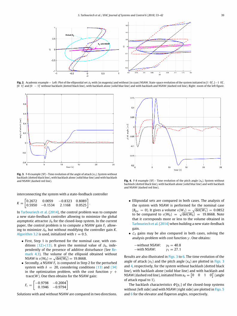
Let us consider to illustrate the approach a small-size exampledescribed by (Ap, Bp, Cp, Dp) = (0.1, 1, 1, 0), with the stabilizing PIcontrol (Ac , Bc , Cc , Dc) = (0, −0.2, 1, −2) and a backlash elementgiven by (ρ, L)= (1.5, 1). Let us first compare the global asymptoticattractor S0 obtained without and with NSAW. Algorithm 3.1 isused both for the analysis of the system without NSAW, and todesign an anti-windup gain Ec , whose the solution is Ec = 0.11.The results are illustrated on Fig. 2. The ellipsoidal sets S0 andtrajectories initiated from several initial conditions in the casewithout backlash (black dotted line), with backlash alone (dashedred line) and with backlash and NSAW (solid blue line) illustratethe positive effect of the NSAW. The simulations without NSAWalso illustrate that the system may converge to a fixed point or toa limit cycle around the origin.

5.2. Four-dimensional unstable F-8 aircraft

Let us now consider an unstable MIMO plant model with fourstates and two inputs. It corresponds to the longitudinal dynamicsof an F-8 aircraft, slightly modified inWu, Grigoriadis, and Packard(2000) to make it unstable. This model has been frequently used inthe past to study the influence of saturating inputs. In this paper,we do not consider saturations but concentrate on the presence ofbacklash phenomenon in the input. Let us then consider the systemdefined by the following matrices

Ap =

⎡⎢⎣−0.8 −0.006 −12 00 −0.014 −16.64 −32.21 −0.0001 −1.5 01 0 0 0

⎤⎥⎦ ;

Bp =

⎡⎢⎣ −19 −3−0.66 −0.5−0.16 −0.5

0 0

⎤⎥⎦ ; Cp =

[0 0 0 10 0 −1 1

]The state variables correspond to the pitch rate, the forward ve-locity, the angle of attack and the pitch angle. The elevator andflaperon angles are the input variables. The output measurementsare set as the pitch angle and the flight path angle (see Wu et al.,2000 for details). External disturbances are considered as acting atthe input of the system, with Bpw = Bp, mimicking the effect ofnoise on the actuator signal.

5.2.1. State-feedback control (SF)This system has already been used in Tarbouriech et al. (2014)

to illustrate the influence of backlash defined as follows

L =

[1 00 1

], ρ =

[0.50.5

]

S. Tarbouriech et al. / IFAC Journal of Systems and Control 6 (2018) 33–42 39

Fig. 2. Academic example— Left: Plot of the ellipsoidal setS0 with (inmagenta) andwithout (in cyan) NSAW. State-space evolution of the system initiated in [1 0]′ , [−1 0]′ ,[0 1]′ and [0 − 1]′ without backlash (dotted black line), with backlash alone (solid blue line) and with backlash and NSAW (dashed red line). Right: zoom of the left figure.

Fig. 3. F-8 example (SF) - Time evolution of the angle of attack (x3). Systemwithoutbacklash (dotted black line), with backlash alone (solid blue line) andwith backlashand NSAW (dashed red line).

interconnecting the system with a state-feedback controller

K =

[0.2672 0.0059 −0.8323 0.80890.5950 −0.1534 2.1168 0.0525

].

In Tarbouriech et al. (2014), the control problem was to computea new state-feedback controller allowing to minimize the globalasymptotic attractor S0 for the closed-loop system. In the currentpaper, the control problem is to compute a NSAW gain Fc allow-ing to minimize S0, but without modifying the controller gain K .Algorithm 3.2 is used, initialized with τ = 0.5.

• First, Step 1 is performed for the nominal case, with con-ditions (12)–(13). It gives the nominal value of S0, inde-pendently of the presence of additive disturbance (See Re-mark 4.3). The volume of the ellipsoid obtained withoutNSAW is v(W0) =

√det(W0) = 19.8668.

• Secondly, a NSAW Fc is computed in Step 2 for the perturbedsystem with δ = 20, considering conditions (13) and (34)in the optimization problem, with the cost function γ +

trace(W ). One then obtains for the NSAW gain:

Fc =

[−0.9798 −0.20040.1946 −0.9794

]Solutions with andwithout NSAW are compared in two directions.

Fig. 4. F-8 example (SF) - Time evolution of the pitch angle (x4). System withoutbacklash (dotted black line), with backlash alone (solid blue line) andwith backlashand NSAW (dashed red line).

• Ellipsoidal sets are compared in both cases. The analysis ofthe system with NSAW is performed for the nominal case(Bpw = 0). It gives a volume v(W1) =

√det(W1) = 0.0852

to be compared to v(W0) =√det(W0) = 19.8668. Note

that it corresponds more or less to the volume obtained inTarbouriech et al. (2014) when building a new state-feedbackgain.

• L2 gains may be also compared in both cases, solving theanalysis problem with cost function γ . One obtains:

−without NSAW: γ0 = 40.8−with NSAW: γ1 = 27.1

Results are also illustrated in Figs. 3 to 6. The time evolution of theangle of attack (x3) and the pitch angle (x4) are plotted in Figs. 3and 4, respectively, for the system without backlash (dotted blackline), with backlash alone (solid blue line) and with backlash andNSAW(dashed red line), initiated from x0 =

[0 0 1 0

]′ (angleof attack equal to 1).

The backlash characteristics Φ[yc] of the closed-loop systemswithout (left side) andwith NSAW (right side) are plotted in Figs. 5and 6 for the elevator and flaperon angles, respectively.

40 S. Tarbouriech et al. / IFAC Journal of Systems and Control 6 (2018) 33–42

Fig. 5. F-8 example (SF) - Backlash characteristics Φ[yc ] for the elevator angle (u1). Left: system without NSAW. Right: system with NSAW.

Fig. 6. F-8 example (SF) - Backlash characteristics Φ[yc ] for the flaperon angle (u2). Left: system without NSAW. Right: system with NSAW.

5.2.2. Dynamic output-feedback control (DOF)

Let us now consider the same F-8 aircraft but controlled by a

dynamic output feedback, issued from Tarbouriech et al. (2011):

Ac =

⎡⎢⎣−4.2676 0.0362 −11.7964 −31.7599−1.7022 −0.0182 2703.8 470.5213−0.9265 −0.0066 −7.0109 6.2734

1 0 0.0801 −3.2993

⎤⎥⎦ ;

Bc =

⎡⎢⎣ 0.3711 1.9263−3217.1 2717.57.6163 −9.18673.2192 0.0801

⎤⎥⎦Cc =

[−0.4485 −0.0045 1.3181 3.19743.9966 0.0144 −7.7734 −10.4292

];

Dc =

[0 00 0

]

S. Tarbouriech et al. / IFAC Journal of Systems and Control 6 (2018) 33–42 41

Fig. 7. F-8 example (DOF) - Time evolution of the angle of attack (x3). Systemwithout backlash (dotted black line), with backlash alone (solid blue line) and withbacklash and NSAW (dashed red line).

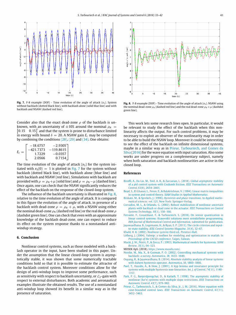
Consider also that the exact dead-zone ρ of the backlash is un-known, with an uncertainty of ±10% around the nominal ρN =[0.15 0.15

]′ and that the system is prone to disturbance limitedin energy with bound δ = 20. A NSAW gain Ec may be computedby combining the conditions (28), (29) and (34). One obtains:

Ec =

⎡⎢⎣ −18.6757 −2.9305−421.7373 −119.8615

1.7229 −0.03572.0566 0.7154

⎤⎥⎦The time evolution of the angle of attack (x3) for the system ini-tiated with x3(0) = 1 is plotted in Fig. 7 for the system withoutbacklash (dotted black line), with backlash alone (blue line) andwith backlash and NSAW (red line). Simulations with backlash areprovidedwithρ = ρN+µ (solid line) andρ = ρN−µ (dashed line).Once again, one can check that the NSAW significantly reduces theeffect of the backlash on the response of the closed-loop system.

The influence of the backlash uncertainty is illustrated in Fig. 8,relative to the time evolution of the angle of attack. It is comparedin this figure the evolution of the angle of attack, in presence of abacklash with dead-zone ρ = ρN + µ, with a NSAW using eitherthenominal dead-zoneρN (dashed red line) or the real dead-zoneρ

(dashdot green line). One can check that evenwith an approximateknowledge of the backlash dead-zone, one can expect to reduceits effect on the system response thanks to a nonstandard anti-windup strategy.

6. Conclusion

Nonlinear control systems, such as those modeled with a back-lash operator in the input, have been studied in this paper. Un-der the assumption that the linear closed-loop system is asymp-totically stable, it was shown that some numerically tractableconditions hold so that it is possible to estimate the attractor ofthe backlash control system. Moreover conditions allow for thedesign of anti-windup loops to improve some performance, suchas sensitivity with respect to backlash uncertainty, orL2-gain withrespect to external disturbances. Both academic and aeronauticalexamples illustrate the obtained results. The use of a nonstandardanti-windup loop showed its benefit in a similar way as in thepresence of saturation.

Fig. 8. F-8 example (DOF) - Time evolution of the angle of attack (x3). NSAW usingthe nominal dead-zone ρN (dashed red line) and the real dead-zone ρN +µ (dashdotgreen line).

This work lets some research lines open. In particular, it wouldbe relevant to study the effect of the backlash when this non-linearity affects the output. For such control problems, it may benecessary to exploit an observer of the nonlinearity map in orderto be able to build the NSAW loop. Moreover it could be interestingto see the effect of the backlash on infinite dimensional systems,maybe in a similar way as in Prieur, Tarbouriech, and Gomes daSilva (2016) for thewave equationwith input saturation. Also someworks are under progress on a complementary subject, namelywhen both saturation and backlash nonlinearities are active in theclosed loop.

References

Bisoffi, A., Da Lio, M., Teel, A. R., & Zaccarian, L. (2018). Global asymptotic stabilityof a pid control system with Coulomb friction. IEEE Transactions on AutomaticControl, 63(8), 2654–2661.

Boyd, S., El Ghaoui, L., Feron, E., & Balakrishnan, V. (1994). Linearmatrix inequalitiesin system and control theory. SIAM Studies in Applied Mathematics.

Brokate, M., & Sprekels, J. (1996). Hysteresis and phase transitions. In Applied mathe-matical sciences: vol. 121, New York: Springer-Verlag.

Corradini, M. L., & Orlando, G. (2002). Robust stabilization of nonlinear uncertainplants with backlash or dead zone in the actuator. IEEE Transactions on ControlSystems Technology, 10(1), 158–166.

Ferrante, F., Gouaisbaut, F., & Tarbouriech, S. (2018). On sensor quantization inlinear control systems: Krasovskii solutions meet semidefinite programming.IMA Journal of Mathematical Control and Information, submitted for publication.

Jayawardhana, B., Logemann, H., & Ryan, E. P. (2011). The circle criterion and input-to-state stability. IEEE Control Systems Magazine, 31(4), 32–67.

Khalil, H. K. (2002). Nonlinear systems third ed., Prentice-Hall.Löfberg, J. (2004). Yalmip: a toolbox for modeling and optimization in matlab. In

Proceedings of the CACSD conference. Taipei, Taiwan.Macki, J. W., Nistri, P., & Zecca, P. (1993). Mathematical models for hysteresis. SIAM

Review, 35(1), 94–123.MOSEK ApS. (2018). https://www.mosek.com/.Nordin, M., Ma, X., & Gutman, P. O. (2002). Controlling mechanical systems with

backlash: a survey. Automatica, 38, 1633–1649.Ouyang, R., & Jayawardhana, B. (2014). Absolute stability analysis of linear systems

with duhem hysteresis operator. Automatica, 50, 1860–1866.Paré, T., Hassibi, A., & How, J. (2001). A kyp lemma and invariance principle for

systems with multiple hysteresis non-linearities. Int. J. of Control, 74(11), 1140–1157.

Park, P. G., Banjerdpongchai, D., & Kailath, T. (1998). The asymptotic stability ofnonlinear (lur’e) systems with multiple slope restrictions. IEEE Transactions onAutomatic Control, 43(7), 979–982.

Prieur, C., Tarbouriech, S., & Gomes da Silva, Jr., J. M. (2016). Wave equation withcone-bounded control laws. IEEE Transactions on Automatic Control, 61(11),3452–3463.

42 S. Tarbouriech et al. / IFAC Journal of Systems and Control 6 (2018) 33–42

Tarbouriech, S., Garcia, G., Gomes da Silva, Jr., J. M., & Queinnec, I. (2011). Stabilityand stabilization of linear systems with saturating actuators. London: Springer.

Tarbouriech, S., Prieur, C., & Queinnec, I. (2010). Stability analysis for linear sys-tems with input backlash through sufficient lmi conditions. Automatica, 46(11),1911–1915.

Tarbouriech, S., Queinnec, I., & Prieur, C. (2014). Stability analysis and stabilizationof systems with input backlash. IEEE Transactions on Automatic Control, 59(2),488–494.

Taware, A., & Tao, G. (2003). Control of sandwich nonlinear systems. In Lecture notesin control and information sciences, vol. 288. Berlin: Springer-Verlag.

Teel, A. R., & Praly, L. (2000). A smooth lyapunov function from a class-kl estimateinvolving two positive semidefinite functions. ESAIM. Control, Optimisation andCalculus of Variations, 5, 313–367.

Wu, F., Grigoriadis, K. M., & Packard, A. (2000). Anti-windup controller designusing linear parameter-varying controlmethods. International Journal of Control,73(12), 1104–1114.

Zaccarian, L., & Teel, A. R. (2011).Modern anti-windup synthesis. Princeton: PrincetonUniversity Press.