Working Paper Series in

ENVIRONMENTAL

& RESOURCE

ECONO:M:ICS

Nonrenewability in Forest Rotations: Implications for Economic and

Ecosystem Sustainability

Jon D. Erickson, Duane Chapman, Timothy J. Fahey, and Martin J. Christ

June 1997

• ..

ERE 97-01 CORNELL WP97-08 UNIVBRSITY

It is the Policy ofCornell University actively to support equality ofeducational and employment opportunity. No person shall be denied admission to any educational program or activity or be denied employment on the basis of any legally prohibited discrimination involving, but not limited to, such factors as race, color, creed, religion, national or ethnic origin, sex, age or handicap. The University is committed to the maintenance of affirmative action programs which will assure the continuation of such equality of opportunity.

..

[

~ I

Nonrenewability in Forest Rotations:

Implications for Economic and Ecosystem Sustainability

By JON D. ERICKSON, DUANE CHAPMAN, TIMOTHY J. FAHEY, AND

MARTIN J. CHRIST"

• Erickson: Department of Economics, Rensselaer Polytechnic Institute, Troy, NY 12180-3590; Chapman: ­Department of Agricultural, Resource, and Managerial Economics, Cornell University, Ithaca, NY 14853-7801; Fahey: Department of Natural Resources, Cornell University, Ithaca, NY 14853-7801; Christ: Department of Biology, West Virginia University, Morgantown, WV 26506. Research supported by the Department of Agricultural, Resource, and Managerial Economics, Cornell University, during Erickson's doctoral studies.

Nonrenewability in Forest Rotations:

Implications for Economic and Ecosystem Sustainability

The forest rotations problem has been considered by generations of

economists, including Fisher (1930), Boulding (1966), and Samuelson

(1976). Traditionally, the forest resource across all future harvest

periods is assumed to grow without memory of past harvest periods.

This paper integrates economic theory and intertemporal ecological

mechanics, linking current harvest decisions with future forest growth,

financial value, and ecosystem health. Results and implications of a

nonrenewable forest resource are reported. (JEL Q23, C61, D92)

-

1

Traditional financial models of the forest resource assume perfect

renewability in forest growth following infinite optimal rotations of constant

length. Forest ecology, however, suggests that rotations can affect future growth,

product quality, and forest health. For instance, alteration of successional sequences,

nutrient cycles, and other components of ecosystem function are influenced by

rotation length, harvest intensity, and cutting frequency. These cross-harvest

interactions suggest a nonrenewable forest growth specification, an omission in the

economist's model of the forest which can lead to sub-optimal management

decisions. Section I addresses this omission, leading to the addition of a marginal

benefit of recovery to the traditional optimal rotation decision rule.

In Section II, an integrated forest succession, product, and price model for the

northern hardwood forest ecosystem is developed to evaluate the impact of

increasing density of pioneer species following disturbance on rotation length and

timber profits. The success of early successional species in disturbance-recovery

cycles from short, repetitive rotations have the effect of delaying forest development

and entrance into late successional, higher quality, higher return species.

Accordingly, a missing variable valuing forest recovery is specified and estimated.

Section III presents the results of solving the discrete horizon rotations

problem. From a nonrenewable growth specification a marginal benefit of recovery

emerges and has the effect over traditional models of lengthening forest rotations,

adjusting profits downwards, and valuing the long-term maintenance of ecosystem

processes.

By incorporating ecosystem modeling into traditional forest economics, a

clearer management picture results through capturing the influence of rotation

length and number on forest recovery. Furthermore, cost estimates of moving from ­short-term economic rotations to long-term ecological rotations suggest the level of

incentive required for one aspect of ecosystem management. A net private cost of

2

maintaining ecosystem health emerges and, for public policy purposes, can be

compared to measures of non-timber amenity values and social benefits exhibiting

increasing returns to rotation length.

I. The Marginal Benefit of Recovery

For the commercial forest manager, the principal economic question centers

on harvest timing. The majority of the economic literature on this question is

grounded in the model developed in the 19th century by the German tax collector

Martin Faustmann (1849). Faustmann was concerned with estimating the bare-land

expected profits l of a forthcoming forest. Assuming land is to remain in forestry,

the problem is to solve for rotation length (T) over an infinite stream of future

profits from harvesting a renewable resource.2

Assuming a continuous-time discount factor (e'lil) and a continuously twice

differentiable stand profit function (1t(t)), the choice of an infinite number of

rotation lengths converges to the choice of one constant length (T), and the infinite

horizon profit maximization problem converges to:

(1) Max n =.Kill elil_1

where

1t(t) =P Q(t).

1 The term "value" has been used to represent forest profits (e.g. Clark, 1990) in economics. Here, • "value" is reserved for problems incorporating non-forest amenities and other positive externalities. For example, forest profits include only income from the sale of timber, where forest value would include non-market goods such as aesthics, biodiversity, or recreation. 2 Note: All symbols used throughout the text are also summarized in Appendix A by order and equation of appearance.

3

Stumpage price (P) is assumed to reflect cutting costs and thus equals net price

per unit volume. In the most general case of the multi-species, multi-grade

problem, P represents a matrix of stumpage prices and, likewise, Q(t) models a

matrix of timber volumes across species and quality classes.

Solving (1) produces the following first-order condition, know as the

Faustmann formula:

(2) 7t'(t) = 07t(t) + 0 7t(t) . llt -1e

From (2), a single optimal rotation length (T) maximizes net present value

(IT) by equating the marginal benefit of waiting to the marginal opportunity cost of

delaying the harvest of the current stand (Le., interest forgone on current profit)

plus the marginal opportunity cost of delaying the harvest of all future stands (Le.,

interest forgone on all future profits, often called site value).3

Adaptations and expansions to this model include modeling non-timber

benefits (e.g., Hartman, 1976; Calish et al., 1978; Berek, 1981), multiple-use forestry

(e.g., Bowes and Krutilla, 1989; Snyder and Bhattacharyya, 1990; Swallow and Wear,

1993), stochastic price paths (e.g., Clarke and Reed, 1989; Forboseh et al., 1996),

market structure (e.g., Crabbe and Long, 1989), and uneven aged forestry (e.g.,

Montgomery and Adams, 1995). However, all these improvements in the basic

Faustmann formula share a strong assumption of perfect growth renewability - a

constant growth function (Q(T)) across all future planning periods.

Evidence from the study of forest ecology and management, however,

indicates a strong relationship between rotation length, rotation frequency, and -.'

3 If real stumpage prices are assumed to grow at a rate r, then the Faustmann formula simply becomes: 1t'(t) =(0 - r) 1t(t) + (0 - xl 1t(t). Equation (15) in the empirical analysis introduces price growth.

e(lH)t_l

4

harvest magnitude in current harvest periods, with the growth and maintenance of

the forest in future periods (e.g., Kimmins, 1987, p. 480; Bormann and Likens, 1979,

p. 221). This is particularly the case where natural regeneration seeds the new forest,

or soil renewability is compromised. In the Faustmann framework, this ecological

knowledge implies a forest stand profit function dependent on rotation-time (T) and

rotation-number (i), given constant technology and harvest magnitude.

To illustrate, consider a cubic functional form for undiscounted profit at

constant prices:

Figure 1 illustrates three plots of (3) following a harvest at To assuming

different parameter values for ~l' ~2' and ~3' Suppose T1A is an optimal Faustmann

rotation in the first harvest cycle (i=l). Therefore, a longer rotation in this first cycle

(for instance, TlB) would be sub-optimal as it would decrease the marginal value of

waiting below the sum of first harvest and future harvest opportunity costs.

However, there may be an additional marginal variable to consider in the

first rotation decision. Suppose rotation length in the first harvest cycle influences

the form of the functional stand profit function in subsequent cycles. For instance,

suppose the choice of T1A in cycle i=l results in the profit function 1t(Ti =21 T1A) in

cycle i=2. A longer rotation such as T1B, however, results in a higher profit function

1t(Ti =21 TlB). In this case, a longer first rotation has the benefit of allowing the forest

more time to recover from the initial cut at To. Now, waiting until T1B to harvest

during the first cycle has the benefit of shifting the second cycle curve upwards to -1t(Ti =21 TlB). A sufficiently long first rotation would result in an identical second

rotation profit function. Without taking into account this cross-harvest impact, the

Faustmann solution of T1A would lead to a sub-optimal decision.

5

B

-

FIGURE 1. CUBIC FOREST UNDISCOUNTED PROFIT FUNCTIONS

To incorporate this interaction between current harvest length and

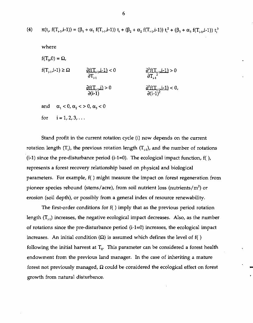
subsequent profit functions consider equation (4). The function f(T i _lI i-I) is added as

a variable to the period i profit function. The level of f(Ti_lI i-I), or ecological impact,

depends on the length of last period's rotation (Ti -1), and the number of rotations

since the first cut at To to take into account any cumulative impacts. It influences

the cubic function parameters (~1I ~2' and ~3) of the stand profit function through an

ecological impact represented by the parameters (X.1I (X.2' and (X.3.

6

where

f(To'O) =0,

af(Ti_1..il > 0 a(i-l)

for i = I, 2, 3, ...

Stand profit in the current rotation cycle (i) now depends on the current

rotation length (TJ, the previous rotation length (Ti _1), and the number of rotations

(i-I) since the pre-disturbance period (i-l=O). The ecological impact function, f( ),

represents a forest recovery relationship based on physical and biological

parameters. For example, f( ) might measure the impact on forest regeneration from

pioneer species rebound (stems/acre), from soil nutrient loss (nutrients/m2) or

erosion (soil depth), or possibly from a general index of resource renewability.

The first-order conditions for f( ) imply that as the previous period rotation

length (Ti _1) increases, the negative ecological impact decreases. Also, as the number

of rotations since the pre-disturbance period (i-l=O) increases, the ecological impact

increases. An initial condition (0) is assumed which defines the level of f( )

following the initial harvest at To' This parameter can be considered a forest health

endowment from the previous land manager. In the case of inheriting a mature

forest not previously managed, 0 could be considered the ecological effect on forest -growth from natural disturbance.

7

Assuming this nonrenewable, rotation-time dependent, stand profit

specification over an infinite horizon, the profit maximization problem becomes:

Under an assumption of perfect renewability, f(To'O) =f(Tl'l) = ... =f(T"",oo) =

0, and the profit maximization problem converges to equation (1), from which the

usual Faustmann result of a constant rotation length in equation (2) is obtained.

Under the assumption of nonrenewability, however, the selection of the

optimal rotation length set (Tj for i = 1,2,3, ...) now considers the impact on each

subsequent period's profits through the addition of a marginal benefit of recovery

(MBR). The marginal benefit of recovery in period i from a rotation length in the

previous period i-I is represented as:

(6) MBR j =af(Tj _1. i-I) {u1T j + u 2T j2 + u 3T j

3} > O.

aTj_1

Thus, balancing the benefits to recovery from longer rotations against the

opportunity costs of delaying current and future harvests will determine the

optimal rotation set.

In the forest ecology literature, Kimmins (1987, p. 480) outlines the distinction

between a Faustmann type rotation where net present value is maximized, and an

ecological rotation, the time required for a site managed with a given technology to

return to the pre-disturbance ecological condition. Figure 2 demonstrates the

concept of an ecological rotation, and the hypothetical case of rotating before a ­successional sequence is completed. Succession is defined as the orderly

replacement over time of one species or community of species by another, resulting

from competitive interactions between them for limited site resources (Marchand,

8

Initial Harvest

Yor-----:iModerate

•~ Regime

Disturbance 3rd Moderate

2nd Moderate Disturbance

Severe Disturbance Regime

Disturbance

J=----+-------+----+---+--------~I----I I I I

To T r 2T

Time

FIGURE 2. KIMMINS' (1987) ECOLOGICAL ROTATION VERSUS SUCCESSIONAL RETROGRESSION

1987, p. 19). The vertical axis of Figure 2 delineates a range from early successional

species (pioneer) to late successional species (climax).

Under a moderate disturbance regime (for instance, stem-harvesting or

selective cutting), T and 2T represent two Faustmann rotations. The declining path

of "backwards" succession is referred to as successional retrogression. For a

moderate disturbance, an ecological rotation is represented by 'P, the time when the

forest recovers to the original successional condition. A more severe disturbance

regime (for instance, whole-tree harvesting or clear-cutting) is also represented -where a longer ecological rotation (TE) would necessarily be required for successional

rebound. Ecological observations also suggest the possibility that severe or repeated

disturbance could shift the biotic community into a different domain in which the

9

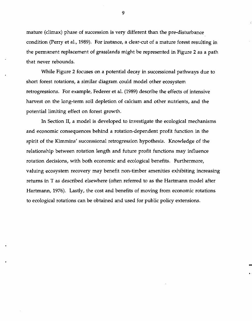
mature (climax) phase of succession is very different than the pre-disturbance

condition (Perry et al., 1989). For instance, a clear-cut of a mature forest resulting in

the permanent replacement of grasslands might be represented in Figure 2 as a path

that never rebounds.

While Figure 2 focuses on a potential decay in successional pathways due to

short forest rotations, a similar diagram could model other ecosystem

retrogressions. For example, Federer et al. (1989) describe the effects of intensive

harvest on the long-term soil depletion of calcium and other nutrients, and the

potential limiting effect on forest growth.

In Section II, a model is developed to investigate the ecological mechanisms

and economic consequences behind a rotation-dependent profit function in the

spirit of the Kimmins' successional retrogression hypothesis. Knowledge of the

relationship between rotation length and future profit functions may influence

rotation decisions, with both economic and ecological benefits. Furthermore,

valuing ecosystem recovery may benefit non-timber amenities exhibiting increasing

returns in T as described elsewhere (often referred to as the Hartmann model after

Hartmann,1976). Lastly, the cost and benefits of moving from economic rotations

to ecological rotations can be obtained and used for public policy extensions.

-

10

II. An Ecological-Economic Model of the Northern Hardwood Forest

To explore the impact of including benefits from recovery on the forest

rotation decision, the Northern Hardwood forest ecosystem is modeled. This forest

type is the dominant hardwood component of the larger Northern Forest stretching

west to northern Minnesota, east through New England, south into parts of the

Pennsylvania Appalachians, and north into Canada.4 It is characterized by sugar

maple (Acer saccharum), American beech (Fagus grandifolia), and yellow birch

(Betula alleghaniensis) predominance, with varying admixtures of other hardwoods

and softwoods. The model includes components to account for forest growth,

pioneer species introduction, conversion from biomass to merchantable timber and

pulpwood, and stumpage price growth.

A. Growth Simulation

The forest growth simulator JABOWA is used to model succession and

growth following a clear-cut in the Northern Hardwood forest. Model

development, parameters, and forest species characteristics are described in

Appendix B. Growth algorithms for each species consist of the following

components (adapted from Botkin et al., 1972).

(7) ~d =G(cr, L, dmax'~) • r(L(I, Z)) • l1(D, Dmin, Dmax) • S(A, 6)

=1 - e-4.64(L - 0.05) (9) r() {shade-tolerant}

=2.24 (1 _e-l.136(L - 0.08») {shade-intolerant} -where L =I e-kZ

4 The hardwood component of the Northern Forest type dominates low to mid elevations in deep, well drained soils.

(8) GO

11

(11) S() =1 - A/e

Equation (7) represents the annual change in species diameter at breast height

(d). Only growth in diameter is modeled because it will be used to predict

merchantable volume (Q) by species and product class for estimating the stand profit

function in equation (1). The function G represents a growth rate equation for each

species under optimal conditions, depending on a solar energy utilization factor (0),

leaf area (L), and maximum values for diameter (dmax) and height (~ax)'

The remaining right-hand side functions act as multipliers to the optimal

growth function to take into account shading, climate, and soil quality. The shading

function, r, is modeled separately for shade-tolerant and intolerant species and

depends on available light to the tree (a function of annual insolation (I) and

shading leaf area (2) 5). The function 11 accounts for the effect of temperature on

photosynthetic rates, and depends on the number of growing degree-days (D) 6 and

species specific minimum and maximum values of D for which growth is possible.

Finally, S is a dynamic soil quality index?

Stochastic dynamics of stand growth enter the model through stem birth and

death subroutines, and are described in more detail in Appendix B. Given this

stochasticity, simulation data vary widely with each model run. Data specific to

defining equations in the remainder of this section can be obtained from the author,

and are based on ten runs (ten 100 m2 plots). This builds an approximately 1/4 acre

-5 A sum of leaf areas of all taller trees on the 100 m2 plot. 6 Approximated by the number of days per year exceeding 40°F, which is in tum approximated by using January and July average temperatures for a site. 7 Dependent on total basal area (A; stem cross-sectional area at breast height) on the plot and maximum basal area (8) under optimal growing conditions.

-

12

plot, which is subsequently expanded to a full acre by assuming each tree represents

four trees per acre.

B. Successional Retrogression

Building on the JABOWA model, the challenge is to incorporate an ecological

mechanism to capture Kimmins' hypothesis of rotation dependent succession and

growth. Such a mechanism is evident in the early succession rebound of pioneer

species. A possible succession of dominant species is represented by Figure 3,

adapted from Marks (1974).

During the first 15 - 20 years following a clear-cut, the recovering forest is

dominated by pioneer species such as raspberry bushes, birches, and pin cherry.

These fast growing, opportunistic species, playa critical role in ecosystem recovery

from a clear-cut by reducing runoff and limiting soil and nutrient loss (Marks, 1974).

However, their initial density will also influence stand biomass accumulation and

Yellow High Birch

Low

60 80 100 120 Time Since Disturbance (Years)

FIGURE 3. NORTHERN HARDWOOD SUCCESSION FOLLOWING CLEAR-CUT

20 40

13

growth of commercial species (Wilson and Jensen, 1954; Marquis, 1969; Mou,

Fahey, and Hughes, 1993; Heitzman and Nyland, 1994).

In this application to the Northern Hardwood forest, pin cherry (Prunus

pensylvanica) is assumed to be the dominant pioneer species. As a particularly fast­

growing, short-lived, shade intolerant species with no commercial value, the effect

of its growth following a clear-cut on forest succession and future harvest profits can

be significant. Tierney and Fahey (1996) demonstrate the influence of short

rotations on the survival of its seeds, and its subsequent germination and growth at

very high density in young stands. This forest ecology research indicates that

pioneer species densities may stabilize at low levels following a 120-year or more

rotation regime (comparable to a Kimmins' ecological rotation), while rotations at

60-year intervals (closer to a Faustmann economic rotation) result in increasing

pioneer species densitities toward a carrying capacity asymptote.

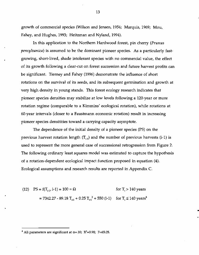
The dependence of the initial density of a pioneer species (PS) on the

previous harvest rotation length (Ti -t ) and the number of previous harvests (i-I) is

used to represent the more general case of successional retrogression from Figure 2.

The following ordinary least squares model was estimated to capture the hypothesis

of a rotation-dependent ecological impact function proposed in equation (4).

Ecological assumptions and research results are reported in Appendix C.

(12) PS =f(T i _JI i-I) =100 =n for Ti > 140 years

=7342.27 - 89.18 Ti_t + 0.25 Ti } + 550 (i-I) for Ti :S 140 years8

•

8 All parameters are significant at a=.lO; R2=O.98; F=65.05.

14

C. Multi-Product, Stochastic Quality Model

The third model component converts stem diameter output from JABOWA

into economic output. The financial value of standing timber depends on age, size,

species, and quality distributions. A typical northern hardwood stand can provide

sawtimber, pulpwood, and firewood. Depending on the market and the land

owners motivations, any combination of these three product classes may be

managed. Equation (13) is used to estimate stand profit.

9 6

(13) 1t(t, P5) = {L L Qs,dd, M, P5] } • PI 5=1 C=l

Profit [1t(t, P5)] is defined at a year following a clear-cut and before the next (t =

0, 1, 2, ... T), given initial pioneer species density (P5). As in equation (1), total

stand profit ($/acre) is the product of a price matrix (PI) and merchantable volume

(Q) for each commercial species (5=1, 2, ,8) and noncommercial species group

(5=9) in each product category (C=I, 2, 6).9 Commercial species numbers

correspond to species listed in Table B2 in Appendix B. Product categories comprise

of grade 1 through 3 timber (C=I-3), below grade sawtimber (C=4), and hardwood

(C=5) and softwood (C=6) pulp. Firewood output was not considered.

Merchantable volume (Q) is modeled on stem diameter (d), provided for each

tree by a growth simulation, and merchantable length (M), which is also modeled

on d. The level of initial pioneer species density (P5) is predicted from equation (12)

based on the previous periods rotation length (Ti _1) and number (i-I). P5 influences

diameter growth through the dynamics of the forest growth simulator, as well as ­9 Note, a matrix of all volumes across species and product classes implicit ifl equation (13) is the same as Q(t) from equation (1).

15

influencing merchantable volume calculations through impacting forest site.

quality. The procedures for converting diameter estimates to merchantable volume

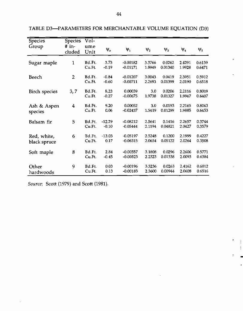
by species and product class are described in detail in Appendix D.

D. Parameterization

Integrating the first three components of the model outlined above,

merchantable stand volumes were generated at 10 year intervals from year 20 to 250,

at initial pioneer species densities of 0, 10, 20, 50, 100, 200, 500, 1000, 2000, and 5000

initial stems per 100 m2 Volume within each species, product class, and year was•

then converted to profit by multiplying a net price matrix of 1995 prices. The initial

distribution of net prices (Po) across product classes and species is summarized in

Table 1. Stand profit for each year was then summarized across all products and

species to generate data for 1t(t, PS) at each PS value run.

TABLE I-INITIAL SAWTIMBER STUMPAGE AND PULPWOOD PRICES (Po)

Below Species Grade Grade 3 Grade 2 Grade 1 Pulp

($/Thousand Board Feet) ($/cord)

Sugar Maple 125 298.30 471.5 650 7 Beech 20 38.15 56.3 75 7 Yellow Birch 50 99.50 149.0 200 7 White Ash 75 182.30 289.5 400 7 Balsam Fir 30 53.10 76.2 100 12 Red Spruce 30 53.10 76.2 100 12 Paper Birch 45 56.55 68.1 80 7 Red Maple 50 83.00 116.0 150 7 Noncommercial 7

Note: Sawtimber prices in each quality class were calculated from ­ranges of stumpage prices reported in NYDEC (1995) for the Adirondack region. Within each range: Min =Below Grade price, 33rd Percentile = Grade 3 price, 66th Percentile =Grade 2 price, and Max =Grade 1 price.

16

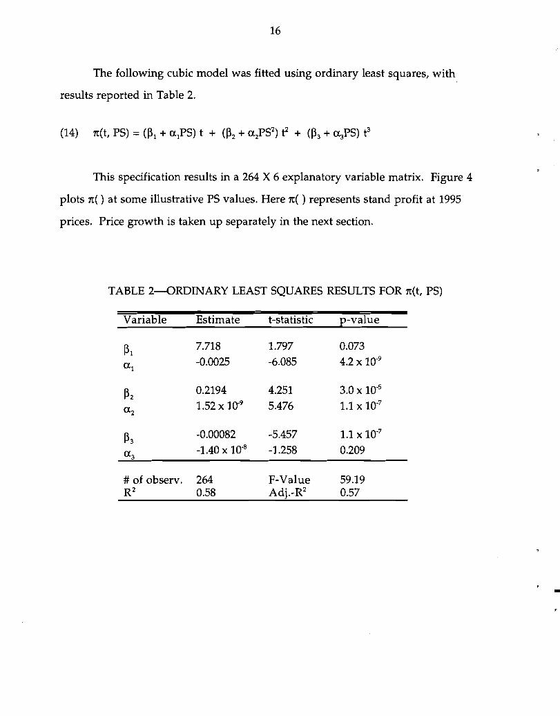
The following cubic model was fitted using ordinary least squares, with

results reported in Table 2.

This specification results in a 264 X 6 explanatory variable matrix. Figure 4

plots n() at some illustrative PS values. Here n( ) represents stand profit at 1995

prices. Price growth is taken up separately in the next section.

TABLE 2-0RDINARY LEAST SQUARES RESULTS FOR n(t, PS)

Variable

~l <Xl

~2 <X 2

~3 <X3

# of observ. R2

Estimate

7.718 -0.0025

0.2194 1.52 X 10-9

-0.00082 -1.40 X 10-8

264 0.58

t-statistic

1.797 -6.085

4.251 5.476

-5.457 -1.258

F-Value Adj.-R2

p-value

0.073 4.2 x 10-9

3.0 x 10-5

1.1 x 10-7

1.1 x 10-7

0.209

59.19 0.57

-

17

4000 3500

(/} PS=-cu 3000 v 'C 2500 tl.t

II') 20000'1 0'1 t""l 1500

1000

--~ v tel 500

iA­0

0 0 0 0 0 0 0-500 \0 0\ N It) 00 ~ -.:l" ~ ~ ~ N N

T

-0 -100 --500 -1000 -5000

FIGURE 4. 1t(T, PS) AT FIVE INITIAL PIONEER SPECIES (PS) DENSITIES

E. Price Growth (P t)

The influences on stumpage prices at the forest stand level are complex. They

might include: timber quality, volume to be cut per acre, logging terrain, market

demand, distance to market, season of year, distance to public roads, woods labor

costs, size of the average tree to be cut, type of logging equipment, percentage of

timber species in the area, end product of manufacture, landowner requirements,

landowner knowledge of market value, property taxes, performance bond

requirements, and insurance costs (NYDEC, 1995). At the macroeconomic level,

exports, mill stocks, and aggregate demand are typically explanatory variables

(Luppold and Jacobsen, 1985). Emerging effects on northeast stumpage prices

include increasing substitution of recycled fibers in paper making, board feet

restrictions on removals in the Pacific Northwest, and continued growth in global -wood demand.

18

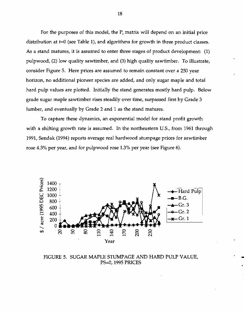
For the purposes of this model, the PI matrix will depend on an initial price

distribution at t=O (see Table 1), and algorithms for growth in three product classes.

As a stand matures, it is assumed to enter three stages of product development: (1)

pulpwood, (2) low quality sawtimber, and (3) high quality sawtimber. To illustrate,

consider Figure 5. Here prices are assumed to remain constant over a 250 year

horizon, no additional pioneer species are added, and only sugar maple and total

hard pulp values are plotted. Initially the stand generates mostly hard pulp. Below

grade sugar maple sawtimber rises steadily over time, surpassed first by Grade 3

lumber, and eventually by Grade 2 and 1 as the stand matures.

To capture these dynamics, an exponential model for stand profit growth

with a shifting growth rate is assumed. In the northeastern U.S., from 1961 through

1991, Sendak (1994) reports average real hardwood stumpage prices for sawtimber

rose 4.3% per year, and for pulpwood rose 1.3% per year (see Figure 6).

-.. C/)

....uOJ 1400 ....

Pot 1200 U 1000 0 ~

800 I.t') 0\ 6000\ .....-- 400 .... OJ

200u !tl 0 ..........

-

0 0 0 0 0 0 0 0f:Ft N I.t') 00 ..... ~ t-... 0 ('Ij ..... ..... ..... N N

Year

-+-Hard Pulp _B.G.

-.-Gr.3

I-o-Gr.2 -.-Gr.l

FIGURE 5. SUGAR MAPLE STUMPAGE AND HARD PULP VALUE, PS=O, 1995 PRICES

19

160

140

8' 120 Average Annual % Change = 4.3%.... II ~ 100 0\ .... - 80[l u -.-Sawtimber";:: 60 ll. _Pulpwood~ 40L.........~~.............. &

Average Annual % Change = 1.3%20

Year

FIGURE 6. NORTHEAST AVERAGE HARDWOOD STUMPAGE ($/MBF) AND HARD PULPWOOD ($/CORD) REAL PRICE GROWTH, 1961-91

As these rates are an average across all quality classes and species, the

following price growth model is assumed to apply to the entire price matrix.

where r(t) =1% if t ::; tL + ~i

=3% if tL + ~i < t ::; tH + ~i

=4% if t> tH + ~i

and ~i = PSI 250

The parameters tL and tH represent the number of years since harvest when

the growing forest stand shifts into higher quality product classes. Following a clear­

cut, the recovering forest stand can only produce pulpwood, a product class where -prices are growing slowly at an exponential growth rate of r(t) = 1%. At tu the stand

shifts into a low quality sawtimber phase (below grade and grade 3), and the

exponential growth rate jumps to 3%. As the stand continues to mature, high

20

quality timber becomes more prevalent until a time tH is reached when timber prices

grow at a rate more characteristic of high quality timber.

As continued short rotations enhance pioneer species abundance, species

competition pushes commercial species development further into the future, thus

delaying the entrance into higher quality product classes. To capture this

successional retrogression hypothesis, a shift variable (.!\J is assumed to add years to

tL and tH depending on pioneer species density at the beginning of each rotation.

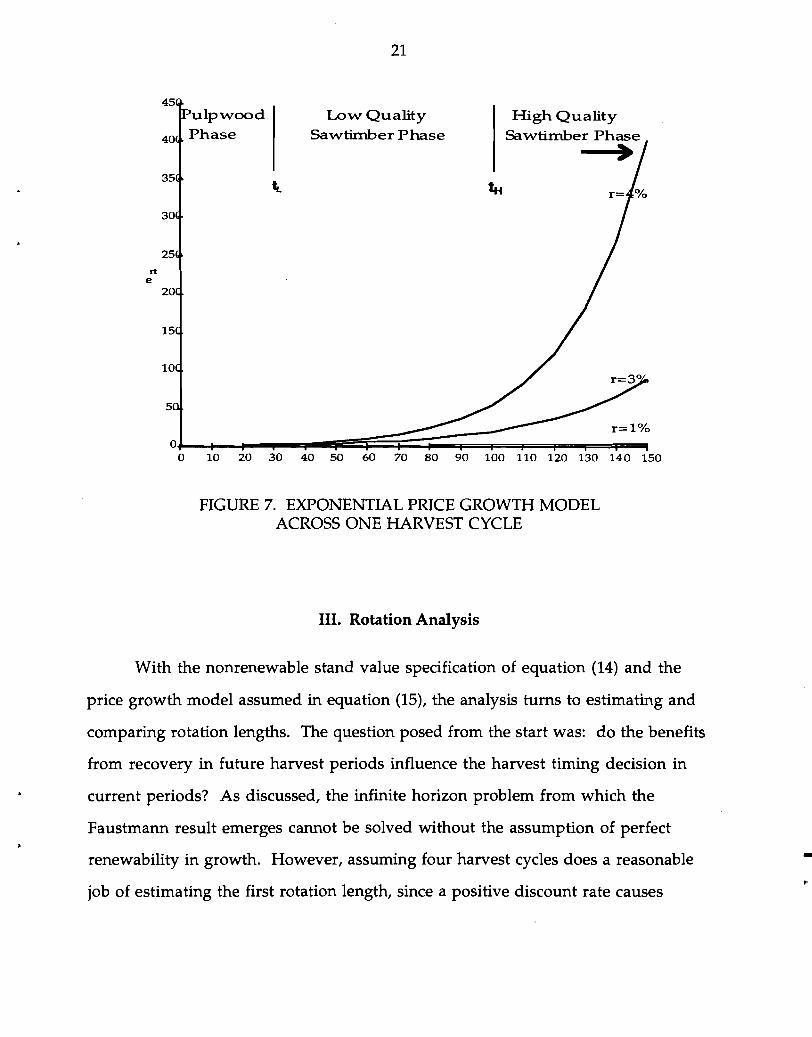
This model is applied by mapping three exponential growth functions over

the planning horizon at each rate. The function is applied as a multiplier to the

initial species by product price matrix (Po), with r depending on t. Figure 7 outlines a

price growth sequence over a 150 year horizon assuming tL =30, tH =100, and PS =O.

In a subsequent rotation, where PS>O, both boundaries between product phases

would shift outward due to a positive .!\j'

The assumption of exponential profit growth is perhaps most relevant to

high quality timber. As global forest productivity declines due to short-sighted

management practices, the supply of high quality timber will fall and its price will

perhaps behave more like a scarcity multiplier of a nonrenewable resource. On a

regional scale, short rotation cycles due to high discount rates may limit high quality

timber supplies. In fact, under a successional retrogression hypothesis and short

rotation lengths, as .!\j continues to increase, the third or fourth harvest may only

yield pulpwood.

-'"

-

21

ulpwood Low Quality High Quality Phase SawtiInber Phase SawtiInber Phase•

rt e

r=l %

oJ-.............-..,...-.-.-pi~==:;~:::::;::~=t===F=""""I"'=~~ o 10 20 30 40 50 60 70 80 90 100 110 120 130 140 150

FIGURE 7. EXPONENTIAL PRICE GROWTH MODEL ACROSS ONE HARVEST CYCLE

III. Rotation Analysis

With the nonrenewable stand value specification of equation (14) and the

price growth model assumed in equation (15), the analysis turns to estimating and

comparing rotation lengths. The question posed from the start was: do the benefits

from recovery in future harvest periods influence the harvest timing decision in

current periods? As discussed, the infinite horizon problem from which the

Faustmann result emerges cannot be solved without the assumption of perfect

renewability in growth. However, assuming four harvest cycles does a reasonable

job of estimating the first rotation length, since a positive discount rate causes

22

profits from harvest cycles beyond four periods to have a negligible effect on the

choice of rotation lengths in earlier periods.

Therefore, assuming cutting costs are internalized in stumpage price and high

labor costs would prohibit thinning young dense stands, the problem is to choose

the rotation set that maximizes the present value of profits over four harvest cycles:

(16) Max I1 =

A. Risk and Choosing an Economic Optimum

The difficulty in solving equation (16) over four periods is that as r varies

within each rotation cycle (from 1% to 3% to 4%), the possibility of multiple

optimums arises. To illustrate, take the case of maximizing profit over just a single

rotation. Figure 8 plots the present value over each price growth phase, assuming

PS=100, 0=5%, tL=30, and tH =100. Two optimums emerge, however, the global

optimum of T=196 is obvious. Under the model assumptions, a 196 year harvest

cycle stabilizes the pin cherry seed bank at "natural" background levels. In this case

the optimal economic rotation length is also an ecological rotation.

However, is this a realistic rotation length? Indeed, at a discount rate of 5% a

rotation length of T=70 is perhaps more characteristic of the end of most commercial

rotations for large landowners in the northern hardwood fo~est.

-

---

23

4000

3500

.- 3000~ ... ~ ~ 2500 QI

;;::s 2000

;>

'E 1500 QI

'" ~ 1000c.

500 T=70years

0 0 0

N ~ 8-Rotation Length (T)

FIGURE 8. PRESENT VALUE OF A SINGLE ROTATION, PS=100, <>=5%, tL=30, AND tH=100

Are managers behaving irrationally? Not when risk and uncertainty are

taken into account. A landholder will not face a profit maximization problem with

perfectly forcasted profits. Risk and uncertainty increase in later periods through

market, government, and environmental variability, effectively raising the discount

rate. For example, as a forest matures its potential for yielding high quality wood

increases, but so does the likelihood of disease, aging effects, or blowdown.

Furthermore, given the pUblic's preference for old growth forests, there may be a

risk of tighter regulations as a stand ages. As present value declines during the

interval 63 < T < 100 at a constant r=3%, the landowner must also evaluate the

expectation that prices will jump (in this case to a growth rate of r=4%) at some age

tHo These types of risks can and should be reflected in the owners discount rate. lO

-10 If stochastic growth was carried through, or stochastic price growth introduced, risk could be modeled with option value methodology by including growth or price variance. Cl~ke and Reed (1989) found an optimal stopping frontier assuming brownian motion for age-dependent growth and geometric brownian motion for price evolution, and an optimal stopping rule under deterministic growth.

24

In the single rotation example of Figure 8, consider the effect of simply raising

the landowners discount rate in the high quality timber phase (T > 100 years) by two

percentage points. One optimum at T=70 results, illustrated in Figure 9. This line of

reasoning is helpful in solving the multi-rotation problem.

350

300 'E... 250I'll

~ ClI 200..: I'll :> 150-c

':V:ClI III

~ c..

I 0 0

~N

Rotation Length (T)

FIGURE 9. PRESENT VALUE OF A SINGLE ROTATION WITH A 2% RISK FACTOR IN PERIODS T>lOO YEARS, PS=lOO, 0=5%, tL=30, AND tH=lOO

-

25

B. The Optimal Rotation Set with Risk, and the Marginal Benefit of Recovery

Assume that because of risk and uncertainty the hypothetical landowner will

maximize profits in either the low quality timber or pulpwood price phases. The

task is to solve equation (16) for Tl' T2, T3 and T4 • Parameter values are as follows:

0=5%, PSo=100, tL=30, and tH =100.

Table 3 outlines the optimal rotation set under two cases. The first is the

successional retrogression hypothesis with 1t(Tj , f(T j _l' i-I)). The second is the

traditional perfectly renewable growth hypothesis with 1t(Tj , PS j =100). The sum of

present value over four periods reveals a 17.5% overestimate of stand profits in the

misspecified problem. Rotation lengths differ by as much as 24 years in the second

cycle, and become longer in future cycles as prices continue to grow exponentially

and profit from future rotations goes to zero. The rotation length for T4 simply

maximizes profits in this cycle.

TABLE 3-FOUR HARVEST PERIOD SOLUTION WITH 2% LONG-RUN RISK FACTOR

Rotation Dependent Renewable Growth Specification Specification

Rotation 1t(TNI f(TN_I , N-1) 1t(TNI PSN=100) (years)

T I 58 40 T2 68 44 T3 70 51 T4 83 70

Net Present $ 400.3/acre $470.2/acre Value

-

26

Compare the first cycle rotation lengths with that of the single rotation

problem represented in Figure 9, where T equaled 70 years. The effect of considering

profits in cycles 2, 3 and 4 at considerably higher prices and identical growth

conditions reduces T1 from 70 to 40 years. This is the result of considering three

period future profits. When successional retrogression is assumed, the shift from 40

to 58 years is the result of including a marginal benefit of recovery.

Differentiating equation (16) by T1 and setting the result to zero yields the first

order condition for T1• The terms can be arranged so that the marginal benefit of

waiting another period equals the marginal cost of delaying first cycle profits plus

the marginal cost of delaying all future profits (site value), as was the case in the

traditional Faustmann formula, and the addition of a marginal benefit of recovery

in the second cycle:

(17)

where

r(T1 ) =r(T2 ) =r(T3 ) =r(T4 ) =r,

R= r-b,

=three period site profit.

At the optimal first cycle rotation (T1=58) the marginal benefit of waiting

another year until harvest is $7.50. It equals the marginal cost of delaying first cycle

profits of $6.30, the marginal cost of delaying the next three harvests (site value) of

$1.70, and the marginal benefit of recovery in future cycles of $0.50. Site value well

exceeds MBR because of the effect of exponential price growth.

-

27

C. Economic and Ecological Indicators under various Discount Rates

The discount rate measures the landowner's opportunity cost. A relatively

low opportunity cost of 0=5% may be characteristic of a large landowner with many

sources of income. For instance, the highest return for a pulp and paper mill in the

northern hardwood forest is in making paper. As long as their mill is fed with a

continuous, inexpensive supply of fiber, management can hold onto timber stands

for speculation in the higher return sawtimber markets, particularly when land is

drawing income between rotations, for instance, through recreationalleasing.ll

Medium opportunity cost in the range of 0=10% may be more characteristic of a

small primary forest product industry or small woodlot owner. A discount rate of

15%, may be characteristic of a landowner not necessarily in the timber industry. In

this case it may be more profitable to use the land for an activity with a shorter

investment horizon, for instance housing development.

Table 4 lists the results of the four cycle optimization when the discount rate

is varied, assuming no risk factor. In the case of high opportunity cost (0=15%), four

pulpwood rotations are optimal at interior solutions of 8, 37, 30 and 30 years with a

total present value of $24/acre. At 0=10% the optimal rotation set occurs in the low

quality sawtimber phase at rotations of 31, 51, 48 and 51 years, all of which are corner

solutions since tL=30, ~1=21, ~2=18 and ~3=21. At 0 =5%, the solution occurs at the

corner of the high quality sawtimber phase.

The sum of present value over four cycles indicates the effect on profit of both

shorter rotations with lower quality products and a higher discount rate. A second

economic indicator, summarizing stand profit at year 105 (the end of the fourth cycle

under 0=15%) with no discounting, indicates only the effect of shorter rotations and ­11 Personal communication with management of Finch, Pruyn and Co. of Glen Fall, N.Y. Finch-Pruyn owns over 160,000 acres of forest in the Adirondack Park of New York State, the majority of which is in hardwoods managed for sawtimber.

28

TABLE 4-THE OPTIMAL 4-CYCLE ROTATION SET AND LONG-RUN ECONOMIC AND ECOLOGICAL HEALTH, VARYING THE DISCOUNT RATE

Optimal 0 Rotation Set 5% 15%10% T1 101 years 31 years 8 years T2 107 51 37 T3 108 48 30 T4 115 51 30

Economic Indicators: Net Present Value $1,122.6/acre $48.6/acre $24.0/acre

Undiscounted Profit @ year 105 $5,909/acre $1,592/acre $500/acre

Ecological Indicators: f(T3' 3) 2,224 stems/ acre 5,277 stems/acre 6,538 stems/acre

39 years 51 years 56 yearstL + Ll3

109 121 126tH + Ll3

lower quality products on profits. Under this second indication, just over one

rotation of high quality sawtimber (at T1=101 and T2=4) produces 2.7 times more

undiscounted profits than three and a half rotations under the low quality

management case, and 10.8 times more undiscounted profits than four full

pulpwood rotations.

Looking at the ecological indicators of the three management scenarios, the

ecological benefits to longer rotations are evident. At the beginning of the fourth

harvest cycle, pioneer species density is 2,224 stems under long rotations, 5,277 stems

under medium length rotations, and 6,538 stems under short rotations. In the

pulpwood harvesting case, entrance into both sawtimber phases is delayed a full 27 ­years by the fourth harvest cycle. The cases where 0=10% and 0=15% demonstrate

the declining trend in successional integrity as suggested by the Kimmins'

29

successional retrogression hypothesis, while the case where 0=5% perhaps

approaches a set of ecological rotations.

D. Single Period Management under Declining Forest Health

Another method to solving the multiple rotations problem is to assume the

values for PSi over subsequent rotations are forest health endowments to new

generations of owners or managers. In other words, a different owner during each

cycle solves a single rotation problem, without consideration of site value or

benefits to recovery. Here, the first order condition within each cycle becomes:

(18)

Again, assuming the landowner will manage either in the low quality

sawtimber or pulpwood price growth phases, the four cycle interior solution for T is

70,80,80, and 83. The result: future landowners must wait longer to maximize

profits due to poorer forest health endowments. Profits continue to increase in later

cycles because of exponential price growth, but not as fast as they would under

perfect growth renewability. By the fourth cycle, the pulpwood price phase is 70

years long, and initial pioneer species density is 3,979 stems/acre.

•

30

E. Ecological Rotations and Valuing Non-Timber Amenities

As was seen in the single period problem, given low constant discount rates

ecological rotations may be economically optimal. Solving equation (16) with a

constant discount rate of 5% yielded the rotation length set of 101, 107, 108 and 115

years with a total present value of $1122.6/acre. Assuming PS=100 and ~i=O across

all cycles (Le., perfect renewability), the optimal set becomes 101, 101, 101 and 116

with a total present value of $1200.2/acre. Here the misspecification error results in

only a 2% overestimate.

These rotation lengths are approaching what might be considered ecological

rotations as described by Kimmins and illustrated in Figure 2. Without risk factored

into the decision and preventively high forest maintenance costs assumed, such

lengths are economically optimal as well. Therefore, the question remains: under

what conditions will landowners rotate forests at 100+ years?

Perhaps including the value of non-timber amenities would make ecological

rotations socially optimal, even at high discount rates. Amenity values that exhibit

increasing returns to rotation length might include recreation value, provision for

certain habitats, and watershed protection.

For example, referring to Table 4, consider the low discount rate solution

(0=5%) and middle discount rate solution (0=10%) as the social and private optimal

rotation sets. Next, evaluating the social rotation set at the private discount rate of

10% results in a total present value of just $5/acre. If a landowner was forced to

rotate at these lengths, this would result in a private loss of $41/acre. However, if

the sum of non-timber amenities exceeds this loss and the landowner experiences

•these benefits directly (for example, hunting or recreational use), then there may be

a private incentive to lengthen rotations.

31

Alternatively, if the amenity values are of a strictly social nature (for example,

watershed protection or biodiversity preservation) then there may be an

opportunity for the government or an environmental group to accomodate the land

owners loss in timber profits through a payment or incentive mechanism (for

example, paying for a conservation easement or providing tax relief). In addition,

alternative silviculture practices such as selective cutting may strike common

ground between the interplay of social and private benefits. For instance, assessing

the ecological impact of economic decisions contributes towards defining and

assessing "new" or "sustainable" forestry, which touts management practices

entrenched in ecological principles with sufficient economic and social policy

returns (Franklin, 1989; Gillis, 1990; Gane, 1992; Fiedler, 1992; Maser, 1994).

IV. Concluding Remarks

Accounting for the ecological recovery of the northern hardwood forest over

a series of harvests was shown to increase rotation lengths over the traditional

Faustmann result. A positive marginal benefit of recovery offsets the marginal costs

of delaying current and future rotations, creating a benefit to delaying rotations

under a nonrenewable stand value growth specification.

Knowledge of benefits to ecosystem recovery can help define both ecological

and economic rotation lengths under various scenarios of ecosystem retrogression.

At one extreme, given low discount rates and risk, relatively long ecological

rotations may be economically optimal. At the other extreme, a site managed with

short rotations motivated by short term profits and a high discount rate may result

in degraded forest stands with low value species - a detriment to long-run ecological ­•

health and social benefits.

32

When considering social welfare from multiple-use management, many

non-timber benefits (Le., recreation, aesthetics, biodiversity) have increasing returns

in rotation length, and thus in forest health recovery. The benefit of recovery was

shown to have a market value, and its inclusion more accurately estimates the

optimal rotation set. Including this benefit, however, may not completely provide

the private incentive to move from ecologically unsustainable to sustainable

rotation lengths and practices, particularly when the net private cost of doing so is

high. However, this net private cost can be compared to benefits from non-timber

amenities and alternative management practices, or to costs of forest maintenance

(Le., thinning undesirable species), providing rationale for social management.

Questions of where to manage along ecological-economic dimensions in a

forest will ultimately depend on a region's spatial ownership pattern, land holder

motivations, policy variables, management costs, timber markets, and ecosystem

characteristics. These modeling results suggest very different economic and

ecological outcomes by varying opportunity cost and ecosystem recovery

assumptions, and suggest a positive benefit to recovery. Estimating economic

benefits across ecological gradients could contribute to valuing non-timber

amenities and developing stewardship policies aimed at managing multiple, spatial

benefits of a forest ecosystem.

-

33

APPENDIX A: LIST OF SYMBOLS (by order of appearance)

Equation 1 T = rotation length (years).

0 = continuous discount rate (%). t = time (years). 1t(t) = forest stand profit function ($/acre) for harvest at time t. IT = total present value of future stream of profits from rotations. P = matrix of net prices per unit volume across species and product

classes. Q(t) = merchantable timber output across species and product classes

at t.

Equation 3

~l' ~2' ~3 = parameters to cubic form of stand profit function (1t(t)).

Equation 4 i = number of forest rotations since predisturbance period (i=O) or

harvest cycle. 1t(ti, f(Ti_1, i-I)) = nonrenewable profit specification. f(Ti_l' i-I) = ecological impact function.

(Xi = fixed impact parameters in nonrenewable profit specification, measuring the impact of f(T i _1, i-I) on the cubic profit function

parameters (~1' ~2' ~3)' n = initial effect on cubic growth function parameters from the

first disturbance (T1); can also be considered as the effect on growth from a natural disturbance regime, for example, from hurricanes or fires.

Equation 6 MBR i = marginal benefit of recovery in harvest cycle i from the choice

of rotation length in the previous harvest cycle (i-I).

Figure 2 r = ecological rotation from moderate disturbance. An ecological

rotation is defined as the time required for a site managed with a given technology to return to the pre-disturbance ecological condition.

= ecological rotation from severe disturbance. -Equations 7 - 11 ~d = annual change in tree diameter. d = diameter at breast height (4.5 feet above ground). h = height.

34

G(O", L, dmax ' ~x) = species growth rate equation under optimal conditions. 0" = solar utilization factor. L = leaf area. dmax = maximum diameter. hmax = maximum height. r(L(I, Z)) = shading function; models effect of shade on optimal growth. L(I, Z) = available light. I = annual solar insolation. Z = shading leaf area, which is the sum of leaf areas of all taller

trees on the 100 m2 plot. = temperature function; models effect of temperature on optimal

growth. = number of growing degree days; approximated by the number

of days per year exceeding 40°F, which is in tum approximated by using January and July average temperatures for a site.

= minimum temperature at which growth is possible. Dmin

Dmax = maximum temperature at which growth is possible. S(A, Q) = soil quality model. A = total basal area per 100 m2

, where basal area is the cross section area at breast height per plot.

e = maximum basal area under optimal growing conditions.

Equation 12 PS = peak pioneer species density following clear cut (stems/acre).

Equation 13 n(t, PS) = rotation time dependent specification of stand value function,

using PS as an estimate of f(T i_1, i-I). S = species (I, 2, ... 8) identified in Table B2 of Appendix B. C = product category (O=below grade sawtimber, l=grade I, 2=grade

2, 3=grade 3, 4=hard pulpwood, 5=soft pulpwood). Qs,c = merchantable volume function by species and quality class. M = merchantable length. PI = matrix of prices across species and product categories at t.

Equation 15 r(t) = exponent in exponential price growth equation. tL = time since harvest when the new stand shifts to an r(t) more

characteristic of low quality sawtimber (C=O and 3) price growth.

= time since harvest when the new stand shifts to an r(t) more ­characteristic of high quality sawtimber (C=l and 2) price growth.

= variable which shifts tL and tH further into the future as PS increases.

35

Equation 17 R =fixed exponential price growth rate (r) less the discount rate (0).

<l> =three period site value for i =2, 3, and 4.

Equation D1 si =species specific site index function. SI(PS) = stand site index, dependent on initial pioneer species density

(PS) (see footnote 17 in Appendix D). bo = parameter to species specific site index function. g = growth rate of reference tree class (i.e. maple-beech-birch

group). =growth rate of slower of faster growing tree class. &

Equation D2 td = minimum top diameter acceptable. all a2, a3 = parameters to merchantable length function.

Equation D3 =parameters to merchantable stem volume function "'i (i = 0, 1,2,3,4,5).

Equations E1 - E3 Gp =potential tree grade. Pk =probability that Gp equals k, where k =grade I, 2, 3, or 4 (below

grade). fj =generalized logistic regression (GLR) model

(j =1,2,3).

Xj1' Xj1' Xj3 = regression coefficients to GLR model. n = uniform random number.

-

36

APPENDIX B: JABOWA FOREST GROWTH AND SUCCESSION SIMULATOR

The JABOWA model is from the popular family of /Igap models" which

simulate growth of individual trees on small plots and disturbance at the forest gap

level. 12 Christ et al. (1995) developed a version of the model in PASCAL to test the

accuracy of the original Botkin et al. (1972) model predictions against forest

inventory data/3 and determine if more recently added modifications improve

those predictions. The model simulates growth of the Northern Hardwood forest,

built on silvical data for the species of the Hubbard Brook Experimental Forest in the

White Mountains of New Hampshire.14

The Christ et al. (1995) model is used to simulate growth on 10 x 10 meter

plots for thirteen species (including two softwoods). Table Bllists species specific

and environmental parameters. Each year, individual trees competing for light

either become established15, grow, or die. Species characteristics and chance

determine the dynamics of these birth-growth-death cycles. As taller trees shade

smaller ones, the amount of shading is dependent on the species' characteristic leaf

number and area, and survival under shaded conditions depends on the shade

tolerance of a species (photosynthetic rates in the shaded environment being higher

in shade-tolerant species vs. intolerant; vice versa under bright conditions). Table

B2 characterizes the relative shade tolerance, and maximum age and height of the

species modeled.

New saplings randomly enter the plot within limits imposed by their relative

shade tolerance and degree-day and soil moisture requirements. Tolerant species,

12 Gap refers to a hole in the forest canopy created by the felling of a tree, naturally or otherwise. 13 One of the important results of this work is that JABOWA tends to grow trees too big, particularly -yellow birch. 14 One of the USDA's Northeast Forest Experiment Stations, and location of the Hubbard Brook Ecosystem Study. 15 Trees enter the modeled stand at a diameter-at-breast-height (DBH) of '0.5 em, a life stage which corresponds to stem establishment rather than birth or germination.

37

yellow and paper birch, and pin cherry are added randomly at the rate of 0-2 stems,

0-13 stems, and 60-75 stems, respectively. In assigning death probabilities for

individual trees, it is assumed that no more than 2% of the saplings of a species will

reach their maximum age. A second mechanism assigns a 1% chance of surviving

10 years for an individual whose annual increment remains below a minimum

value.

TABLE Bl-SPECIES AND ENVIRONMENTAL PARAMETERS IN JABOWA

Species Specific Parameters • Maximum age, diameter, and height • Relation between: height and diameter,

total leaf weight and diameter, rate of photosynthesis and available light, relative growth and climate

• Range of stem establishment requirements • Limit on number of saplings allowed under shading conditions

Abiotic Environment Assumption: • Elevation 549 meters • Soil Depth 3 meters deep • Soil-moisture holding capacity 15 cm/m • Percent rock in soil 5% • Degree days (400 F base) 3,288 0 days • Actual evapotranspiration 542.3 mm H20

•

38

TABLE B2---eHARACTERISTICS OF SPECIES MODELED WITH JABOWA

# Species Shade Maximum Maximum Tolerance Known Age Known

(years) Height (ft.) Commercial 1 Sugar Maple (Acer saccharum) Tolerant 200 132 2 Beech (Fagus grandifolia) Tolerant 300 120 3 Y. Birch (Betula alleghaniensis) Intermed. 300 100 4 White Ash (Fraxinus americana) Intermed. 100 71

Balsam Fir (Abies balsamea) Tolerant 80 60 6 Red Spruce (Picea rubens) Tolerant 350 60 7 Paper Birch (Betula papyrifera) Intolerant 80 60

8 Red Maple (Acer rubrum) Intermed. 150 120

Noncommercial 9 Mountain Maple (Acer spicatum) Tolerant 25 16 9 Striped Maple (A. pensylvanicum) Tolerant 30 33

9 Pin Cherry (Prunus pensylvanica) Intolerant 30 37

9 Chokecherry (P. virginia) Intolerant 20 16 9 Mountain Ash (Sorbus americana) Tolerant 30 16

Source: Adapted from Botkin et al. (1972).

39

APPENDIXC: DYNAMIC PIONEER SPECIES MODEL

Pin cherry (Prunus pensylvanica) is used as a representative pioneer species

to estimate the ecological impact function, f(T i _1, i-1), in equation (4). The

reproduction of pin cherry follows a buried seed strategy. Seed production begins at

a very early age (- 3 years), and are dispersed widely by birds. Some survive in the

soil seed bank for periods of longer than 100 years. Germination occurs only when

the right conditions are present (most significantly, light resulting from a large

forest opening such as that created by severe windstorms or clear-cutting). The I

result in forest management terms: the shorter the forest rotation, the more seeds

survive and germinate, and the denser initial pin cherry stands become in

subsequent rotation-recovery cycles.

Figure C1 presents two forest rotation scenarios of pin cherry rebound,

summarizing the soil seed bank dynamic modeling results of Tierney and Fahey

(1996). Background level in the seed bank is assumed 5 pin cherry seeds/m2 in

stands greater than 170 years old. At the initial disturbance at TO' one stem/m2

becomes established. They further hypothesize that rotations greater than 120 years

may allow enough depletion of the seed bank to stabilize pin cherry germination at

10 stems1m2• At the other extreme, 60 year rotations may eventually triple the size

of the pin cherry soil seed bank, resulting in peak stem densities (stems/m2) of 30 at

T1=61, 42 at T2=121, 48 at T3=181, and approaching a limit of 50 at T4=241.

Table C1 lists data used to estimate equation (12) based on three disturbance

regimes: 60 and 120 year from Figure C1, and 170 year.

-

50

40

,, ,, ,, ~ QJ-::;QJ 40

QJ ~ !U ;:l l:T' m II) - 30e QJ

m-S QJ

..c: 20U

....= ~

10

Disturbance Regimes:

60-year

-- l20-year

, ,\ \

"-­" "

:'" " ,"'

·, ,,·, ,, ,·, ,, , ,I \ , \

,l

50

\I ,\ ,\ , \ \

, \ \

\ \ '. I,

,\

I." I,'.

\ " " " " ,"

I," -­ " " " , "

" " , .'"

"

,," ,", , , , ,, ,, ,,

I\ ,, ,, ,\ , \ ,\

\\ ,\ \

\

~

, , , , , , , , , , , , , , , \ \

100 150 200 250

Years

FIGURE C1. PIN CHERRY REBOUND, 60-YEAR AND 120-YEAR DISTURBANCE REGIMES

TABLE C1-DATA FOR PS =f(T i_l' i-I) ESTIMATION

Initial Pioneer Previous Cycle # of Rotations Species Density Rotation Length Before Current

(PS) (Ti -1) Ti_1 2 (i-I)

100 170 28,900 1 100 170 28,900 2

1000 120 14,400 1 1000 120 14,400 2 -3000 60 3,600 1 4200 60 3,600 2 4800 60 3,600 3 5000 60 3,600 4

41

APPENDIXD: MULTI-PRODUCT, STOCHASTIC QUALITY MODEL16

Species and diameter at breast height (d) are provided for each tree by the

ecology model run. When converting diamter to merchantable volume, stems with

d < 5 inches are discarded. Softwoods with d < 9 inches are considered softwood

pulp (C=6) and hardwoods with d < 11 inches are considered hardwood pulp (C=5).

Noncommercial species (5=9) do not reach sawtimber diameters.

Determining the sawtimber classes (C=1,2,3,4) isn't as straight forward. First a

species specific site index (si) must be computed from a benchmark index (51) for the

maple-beech-birch class which is in turn modeled as a function of PSY This

provides a more accurate growth potential of each species on the site. Defining g as

the growth rate of the general class, and gs as that of the slower or faster growing

class, for nine species groups the following model from Hilt et al. (1989) was

incorporated. Parameter estimates are tabulated in Table D1.

(D1) si = bo + 1.104 51 (PS)

= 110- + 0.906 51 (PS) 1.104

16 The following procedures and equations were programmed in Visual Basic for Microsoft Excel Macros. A 19 page appendix including the code is available from the author. These procedures were originally developed by the USDA Forest Service and have also been incorporated in the NE-TWIGS forest growth model. See Miner et al. (1988) for a general reference to the TWIGS family of models. 17 Site index is a proxy to site quality measured as the height of the dominant canopy species at year 50. Based on eleven JABOWA runs at the PS densities specified above, the following ordinary least squares result was used to predict 51 from Ps: .

51 = 54.90197 - 0.00418 PS

-

42

TABLE D1-PARAMETERS FOR SITE INDEX EQUATION (D1)

Height Group Species included bo in group (see Table B2 for #'s) when g<gs when g>gs

Black cherry-poplar-aspen 9 Elm-ash-cottonwood 4 -1.824 Afaple-beech-birch 1,2,3,7,8 Balsam fir-eastern hemlock 5 1.408 R. spruce-tamarack-other 6,9 -0.800 hardwoods

Note: Of the species in the noncommercial grouping (S=9), pin cherry and striped maple were included in the fastest growing class, and mountain maple and chokecherry were included in the slowest growing class with "other hardwoods". Source: Hilt et al. (1989).

Next a random number is generated and assigned to each stem, and along

with d and si, the potential sawtimber class (or tree grade (Gp»is determined with a

generalized logistic regression (GLR) model as estimated by Yaussey (1993). The GLR

procedure, parameters, and an example are described in Appendix E.

With Gp assigned by stem, actual tree grades (Ga) are then assigned at current

period diameters. Softwoods are either grade 1 or below grade, regardless of current

d. Diameter restrictions for hardwoods include 16 inches for grade 1 and 13 inches

for grade 2 (Yaussey, 1993). For example, a hardwood with G p = 1 and d = 15 would

be assigned Ga = 2.

With quality classes established, merchantable length (M) is calculated in

equation (D2) from si, d, and a new parameter, td (minimum top diameter

acceptable). Restrictions on td are 9,7, and 4 inches for hardwood sawlogs, softwood •

sawlogs, and pulpwood, respectively. Parameter estimates are tabulated in Table D2.

(D2) M = a1 sia2 {I - exp[a3 (d - td)]}

43

TABLE D2-PARAMETERS FOR MERCHANTABLE LENGTH EQUATION (D2)

# Species a1 a2 a3

1 Sugar Maple 21.237 0.182 -0.294 2 Beech 16.430 0.212 -0.328 3 Yellow Birch 18.922 0.176 -0.400 4 White Ash 26.321 0.135 -0.268 5 Balsam Fir 17.394 0.252 -0.326 6 Red Spruce 24.180 0.186 -0.280 7 Paper Birch 18.922 0.176 -0.400 8 Red Maple 22.319 0.149 -0.342 9 Noncommercial 26.129 0.000 -0.493

Source: Yaussy and Dale (1991).

Lastly, within each species and product class, board-feet for sawtimber and

cubic feet for pulpwood18 are estimated from d and M. The following model for

merchantable stem volume (Q) is assumed. Parameter estimates for "'i for board-feet

and cubic feet are tabulated in Table D3.

-

18 When prices are introduced, one cord per 70 cubic feet is assumed for pulpwood volume.

44

TABLE D3-PARAMETERS FOR MERCHANTABLE VOLUME EQUATION (D3)

Species Species Vol-Group # in- ume

eluded Unit "'0 "'1 "'2 "'3 "'4 "'5

Sugar maple 1 Bd.Ft. 3.73 -0.00182 3.3766 0.0262 2.4291 0.6139 Cu.Ft. -0.19 -0.01171 1.8949 0.01340 1.9928 0.6471

Beech 2 Bd.Ft. -0.84 -0.01207 3.0043 0.0419 2.3951 0.5912 Cu.Ft. -0.60 -0.00711 2.2693 0.01399 2.0190 0.6518

Birch species 3,7 Bd.Ft. 8.23 0.00039 3.0 0.0206 2.2116 0.8019 Cu.Ft. -0.27 -0.00675 1.9738 0.01327 1.9967 0.6407

Ash & Aspen 4 Bd.Ft. 9.20 0.00052 3.0 0.0193 2.2165 0.8043

species Cu.Ft. 0.06 -0.02437 1.5419 0.01299 1.9885 0.6453

Balsam fir 5 Bd.Ft. -12.29 -0.08212 2.5641 0.1416 2.2657 0.3744 Cu.Ft. -0.10 -0.05444 2.1194 0.04821 2.0427 0.3579

Red, white, 6 Bd.Ft. -13.03 -0.05197 2.5248 0.1200 2.1999 0.4227

black spruce Cu.Ft. 0.17 -0.06315 2.0654 0.05122 2.0264 0.3508

Soft maple 8 Bd.Ft. 2.84 -0.00557 3.1808 0.0296 2.2606 0.5771 Cu.Ft. -0.45 -0.00523 2.2323 0.01338 2.0093 0.6384

Other 9 Bd.Ft. 0.03 -0.00196 3.3236 0.0263 2.4162 0.6012 Cu.Ft. 0.13 -0.00183 2.3600 0.00944 2.0608 0.6516hardwoods

Source: Scott (1979) and Scott (1981).

-

45

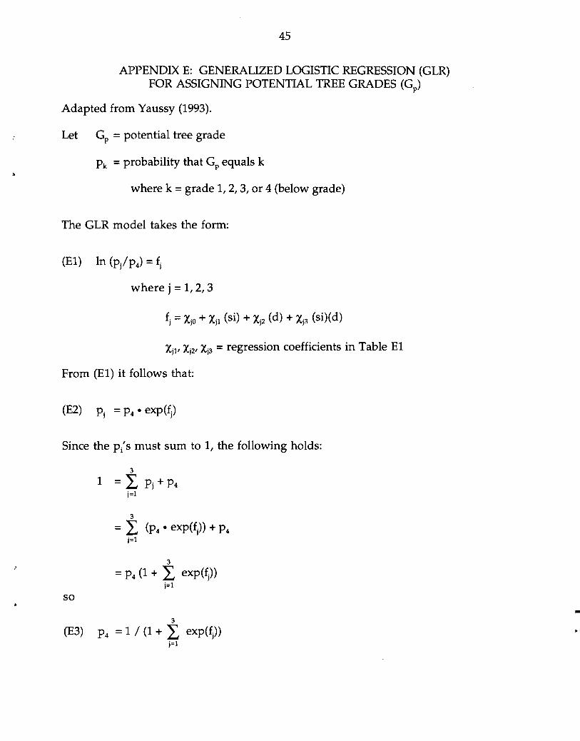
APPENDIX E: GENERALIZED LOGISTIC REGRESSION (GLR) FOR ASSIGNING POTENTIAL TREE GRADES (Gp)

Adapted from Yaussy (1993).

Let Gp = potential tree grade

Pk =probability that Gp equals k

where k =grade I, 2, 3, or 4 (below grade)

The GLR model takes the form:

where j =1,2,3

fj =XjD + Xj1 (si) + Xj2 (d) + Xj3 (si)(d)

Xj1' Xj2' Xj3 =regression coefficients in Table El

From (El) it follows that:

Since the p/s must sum to I, the following holds:

1 =L 3

Pi + P4 j=l

3

=L (P4 • exp(fj)) + P4 j=l

= P4 (1 + L3

exp(fj))

j=l

so •

(E3) P4 = 1 / (1 + L3

exp(fj)) .' j=l

46

TABLE E1-COEFFICIENTS FOR THE GENERALIZED LOGISTIC REGRESSIONS

Species Group

Commer­cial species included

XiD Xu Xi2 j3

Ash 4 1 2 3

-1.6880 3.0552 4.3884

0.0145 -0.0235 -0.0265

0.0770 -0.1620 -0.2638

-0.00090 0.00102 0.00155

Beech 2 1 2 3

-3.7807 -4.0959 0.7484

-0.0229 0.0167

-0.0173

0.0191 0.1002

-0.0890

0.00023 -0.00160 0.00028

Birch 3,7 1 2 3

-7.2202 -3.5818 2.9962

0.0313 0.0285

-0.0363

0.2471 0.0987

-0.2099

-.00210 -0.00154 0.00205

Hemlock 5,6 1 0.6158 -0.0033 -0.0057 0.00012

Red Maple

8 1 2 3

-4.8396 -2.2768 1.9865

0.0096 0.0144

-0.0206

0.1327 0.0932

-0.1169

-0.00113 -0.00176 0.00052

Sugar Maple

1 1 2 3

-4.1101 -1.1156 1.7617

0.0141 0.0062

-0.0056

0.1198 0.0164

-0.0902

-0.00104 -0.00073 -0.00042

Source: Yaussey (1993, p. 7-8, Table 3).

The proportion of trees in one of the four potential tree grade classes (two

classes for softwoods) is computed from equations (E2) and (E3). To illustrate how

these probabilities are computed and applied, consider an example of a group of

sugar maples with DBH (d) of 15 inches and a site index (si) of 60 feet. Using

parameter values for sugar maple from Table E1, first compute: ­exp(f1) = exp(-4.1101 + 0.0141 (si) + 0.1198 (d) - 0.00104 (si)(d))

= 0.0904

47

exp(f2)

exp(f3)

= 0.3152

= 0.7369

L exp(9 = 1.1425

Next, employing equation (E3), the proportion of trees of this species,

diameter, and site index with a Gp equal to below grade is:

P4 = (1 + 1.1425)-1 = 0.4667

The remaining probabilities for grades I, 2, and 3 are then computed from equation

(E2) as follows:

PI = P4 • exp(f1) = 0.4667 • 0.0904 = 0.0422

P2 = 0.1471

P3 = 0.3439

To apply these probabilities, a uniform random number is generated (n) for

each sawtimber stem. In this example, for each sugar maple stem with d=15 in a

stand with a sugar maple site index of 60, a potential tree grade would be assigned

based on cumulative probabilities as follows:

G =1p

G =2p

G =3p

G =4p

if

if

if

if

o~ n ~ 0.0422,

0.0422 < n ~ 0.1893,

0.1893 < n ~ 0.5332, and

0.5332 < n ~ 1.

-•

48

REFERENCES

Berek, P. "Optimal Management of Renewable Resources with Growing Demand and Stock Externalities." Journal of Environmental Economics and Management, 1981, 8, pp. 105-117.

Borman, F. Herbert and Likens, Gene E. Pattern and Process in a Forested Ecosystem: disturbance, development, and the steady state based on the Hubbard Brook ecosystem study. New York: Springer-Verlag, 1979.

Botkin, Daniel B.; Janak, James F. and Wallis, James R. "Some Ecological Consequences of a Computer Model of Forest Growth." Journal of Ecology, 1972, 60, pp. 948-972.

Boulding, Kenneth E. Economic analysis. New York, NY: Harper, 1966.

Bowes, Michael D. and Krutilla, John V. Multiple-use management: the economics of public forestlands. Washington, DC: Resources for the Future, 1989.

Calish, Steven; Fight, Roger D. and Teeguarden, Dennis E. "How Do Nontimber Values Affect Douglas-Fir Rotations?" Journal of Forestry, April 1978, 76, pp. 217­221.

Christ, Martin; Siccama, Thomas G.; Botkin, Daniel B. and Bormann, F. H. "Comparison of Stand-Dynamics at the Hubbard Brook Experimental Forest, New Hampshire, with Predictions of JABOWA and Other Forest-Growth Simulators." Institute of Ecosystem Studies, Millbrook, NY, 1995 (available from authors).

Clark, Colin W. Mathematical Bioeconomics: the optimal management of renewable resources. New York, NY: John Wiley & Sons, 1990.

Clarke, Harry R. and Reed, William J. "The Tree-Cutting Problem in a Stochastic Environment: the Case of Age-Dependent Growth." Journal of Economic Dynamics and Control, 1989, 13, pp. 569-595.

Crabbe, Phillipe H. and Van Long, Ngo. "Optimal Forest Rotation Under Monopoly and Competition." Journal of Environmental Economics and Management, 1989, 17, pp. 54-65.

Faustmann, Martin. "On the Determination of the Value Which Forest Land and Immature Stands Possess for Forestry," 1849, in M. Gane, ed., Martin Faustmann ­and the evolution of discounted cash flow. Oxford, UK: Oxford Institute Paper ..42,1968.

49

Federer, C. Anthony; Hornbeck, James W.; Tritton, Louise M.; .Martin, C. Wayne; Pierce Robert S. and Smith, C. Tattersall. "Long-Term Depletion of Calcium and Other Nutrients in Eastern US Forests." Environmental Management, 1989, 13(5), pp. 593-601.

Fiedler, C. "New Forestry: Concepts and Applications." Western Wildlands, 1992, 17(4), pp. 2-7.

Fisher, Irving. The theory of interest. New York, NY: Macmillan, 1930.

Forboseh, Philip F.; Brazee, Richard J. and Pickens, James B. "A Strategy for Multiproduct Stand Management with Uncertain Future Prices." Forest Science, 1996,42(1), pp. 58-66.

Franklin, J. "Toward a New Forestry." American Forests, Nov./Dec 1989.

Gane, M. "Sustainable Forestry." Commonwealth Forestry Review Volume, 1992, 71(2), pp. 83-90.

Gillis, A.M. "The New Forestry: An ecosystem approach to land management," Bioscience, 1990,40(8), pp. 558-562.

Hartman, Richard. "The Harvesting Decision when a Standing Forest has Value." Economic Inquiry, March 1976,4, pp. 52-58.

Heitzman, Eric and Nyland, Ralph D. "Influences of Pin Cherry (Prunus pensylvanica L. f.) on Growth and Development of Young Even-aged Northern Hardwoods." Forest Ecology and Management, 1994,67, pp. 39-48.

Hilt, Don; Teck, Rich and Fuller, Les. "Site Index Conversion Equations for the Northeast." USDA Forest Service, Northeastern Forest Experiment Station (Delaware, OH), File Report Number I, Research Work Unit FS-NE-4153, 1989.

Kimmins, J. P. Forest Ecology. New York, NY: Macmillan, 1987.

Luppold, William G. and Jacobsen, Jennifer M. "The Determinants of Hardwood Lumber Price." USDA Forest Service, Northeastern Forest Experiment Station (Broomall, PA), Research Paper NE-558, 1985.

Marchand, Peter J. North Woods: an inside look at the nature of forests in the Northeast. Boston, MA: Appalachian Mountain Club, 1987. -

Marks, Peter L. "The Role of Pin Cherry (Prunus pensylvanica L.) in the Maintenance of Stability in Northern Hardwood Ecosystems." Ecological Monographs, 1974, 44(1), pp. 73-88.

50

Marquis, D. A. "Thinning in Young Northern Hardwoods: 5 year results." USDA Forest Service, Northeast Forest Experiment Station (Broomall, PA), Research Paper 139, 1969.

Maser, C. Sustainable Forestry: philosophy, science, and economics, Delray Beach, FL: St. Lucie Press, 1994.

Miner, Cynthia L.; Walters, Nancy R. and Belli, Monique L. "A Guide to the TWIGS Program for the North Central United States." USDA Forest Service, North Central Forest Experiment Station (St. Paul, MN), General Technical Report NC-125, 1988.

Montgomery, Claire A. and Adams, Darius M. "Optimal Timber Management Policies," in Daniel W. Bromley, ed., The handbook of environmental economics. Oxford, UK: Blackwell, 1995.

Mou, Pu; Fahey, Timothy J. and Hughes, Jeffrey W. "Effects of Soil Disturbance on Vegetation Recovery and Nutrient Accumulation Following Whole-tree Harvest of a Northern Hardwood Ecosystem, HBEF." Journal of Applied Ecology, 1993,30, pp. 661-675.

NYDEC. "Stumpage Price Report:' Division of Lands and Forests, New York State Department of Environmental Conservation (Albany, NY), Number 46, January 1995.

Perry, D. A.; Amaranthus, M. P.; Borchers, J. Go; Borchers S. L. and Brainerd, R. E. "Bootstrapping in Ecosystems." Bioscience, April 1989, 39(4), pp. 230-237.

Samuelson, Paul A. "Economics of Forestry in an Evolving Society." Economic Inquiry, December 1976, 14, pp. 466-91.

Scott, Charles T. "Northeastern Forest Survey Board-Foot Volume Equations." USDA Forest Service, Northeastern Forest Experiment Station (Broomall, PA), Research Note NE -271, 1979.

_____,. "Northeastern Forest Survey Revised Cubic-Foot Volume Equations." USDA Forest Service, Northeastern Forest Experiment Station (Broomall, PA), Research Note NE-304, 1981.

Sendak, Paul E. "Northeastern Regional Timber Stumpage Prices: 1961-91:' USDA Forest Service, Northeastern Forest Experiment Station (Radnor, PA), Research Paper NE-683, January 1994.

Snyder, Donald L. and Bhattacharyya, Rabindra N. "A More General Dynamic Economic Model of the Optimal Rotation of Multiple-Use Forests." Journal of Environmental Economics and Management, 1990, 18, pp. 168-175.

51

Swallow, Stephen K. and Wear, David N. "Spatial Interactions in Multiple-Use Forestry and Substitution and Wealth Effects for the Single Stand." Journal of Environmental Economics and Management, 1993, 25, pp. 103-120.

Tierney, Geraldine L. and Fahey, Timothy J. "Soil Seed Bank Dynamics of Pin Cherry in Northern Hardwoods Forest, New Hampshire, USA." Department of Natural Resources, Cornell University (Ithaca, NY), Working Paper, 1996.

Wilson, Jr., R. W. and Jenson, V. S. "Regeneration After Clear-Cutting Second­Growth Northern Hardwoods." USDA Forest Service, Northern Forest Experiment Station, Station Note 27, 1954.

Yaussy, Daniel A. and Dale, Martin E. "Merchantable Sawlog and Bole-Length Equations for the Northeastern United States." USDA Forest Service, Northeastern Forest Experiment Station (Radnor, PA), Research Paper NE-650, 1991.

Yaussy, Daniel A. "Method for Estimating Potential Tree-Grade Distributions for Northeastern Forest Species." USDA Forest Service, Northeastern Forest Experiment Station (Radnor, PA), Research Paper NE-670, March 1993.

-

WPNo IilIe

97-07 Is There an Environmental Kuznets Curve for Energy? An Econometric Analysis

1 97-06 A Comparative Analysis of the Economic Development of

Angola and Mozamgbique

97-05 Success in Maximizing Profits and Reasons for Profit Deviation on Dairy Farms

97-04 A Monthly Cycle in Food Expenditure and Intake by Participants in the U.S. Food Stamp Program

97-03 Estimating Individual Farm Supply and Demand Elasticities· Using Nonparametric Production Analysis

97-02 Demand Systems for Energy Forecasting: Practical Considerations for Estimating a Generalized Logit Model

97-01 Climate Policy and Petroleum Depletion

96-22 Conditions for Requiring Separate Green Payment Policies Under Asymmetric Information

96-21 Policy Implications of Ranking Distributions of Nitrate Runoff and Leaching by Farm, Region, and Soil Productivity

96-20 The Impact of Economic Development on Redistributive and Public Research Policies in Agriculture

96-19 Penn State Comell Integrated Assessment Model

96-18 The G3 Free Trade Agreement: A Preliminary Empirical Assessment

96-17 The G3 Free Trade Agreement: Member Countries' Agricultural Policies and its Agricultural Provisions

96-16 Developing a Demand Revealing Market Criterion for Contingent Valuation Validity Tests

96-15 Economies of Size in Water Treatment vs. Diseconomies of Dispersion for Small Public Water Systems

Author(s)

Agras, J. and D. Chapman

Kyle, S.

Tauer, L. and Z. Stefanides

Wilde, P. and C. Ranney

Stefanides, Z. and L. Tauer

Weng, W. and T.D. Mount

Khanna, N. and D. Chapman

Boisvert, R.N. and J.M. Peterson

Boisvert, R.N., A.Regmi and T.M. Schmit

de Gorter, H. and J.F.M. Swinnen

Barron, E.J., D. Chapman, J.F. Kasting, N. Khanna, A.Z. Rose and P.A. Schultz

R. Arguello and S. Kyle

Arguello, R. and S. Kyle

Rondeau, D., G.L. Poe and W.D. SChulze -Boisvert, R.N. and T.M. Schmit

0­

To order single copies ofARME pUblications, write to: Publications, Department ofAgricultural, Resource, and Managerial Economics, Warren Hall, Cornell University, Ithaca, NY 14853-7801.