nonparametric testing for asymmetric information - singapore
TRANSCRIPT

Nonparametric Testing for Asymmetric Information
Liangjun Su, Martin Spindler
School of Economics, Singapore Management University ([email protected]) Ludwig—Maximilians—University and Max Planck Society, Germany
First version: July 23, 2010
This version: November 28, 2012
Abstract
Asymmetric information is an important phenomenon in many markets and in particular in
insurance markets. Testing for asymmetric information has become a very important issue in
the literature in the last two decades. Almost all testing procedures that are used in empirical
studies are parametric, which may yield misleading conclusions in the case of misspecification
of either functional or distributional relationships among the variables of interest. Motivated
by the literature on testing conditional independence, we propose a new nonparametric test
for asymmetric information which is applicable in a variety of situations. We demonstrate
that the test works reasonably well through Monte Carlo simulations and apply it to an
automobile insurance data set and a long term care insurance data set. Our empirical results
consolidate Chiappori and Salanié’s (2000) findings that there is no evidence for the presence
of asymmetric information in the French automobile insurance market. While Finkelstein
and McGarry (2006) find no positive correlation between risk and coverage in the long term
care insurance market in the US, our test detects asymmetric information using only the
information that is available to the insurance company and our investigation of the source
of asymmetric information suggests some sort of asymmetric information that is related to
risk preferences as opposed to risk types and thus lends support to Finkelstein and McGarry
(2006).
Keywords: Asymmetric information, Automobile insurance, Long term care insurance,
Conditional independence, Distributional misspecification, Functional misspecification, Non-
linearity, Nonparametric test.
JEL classification codes: C12, C14, D82, D86, G22.
1 Introduction
Since Akerlof (1970) the notion of asymmetric information, comprising adverse selection and moral
hazard, has been explored at a rapid pace. At the same time people observed a wide gap between
the theoretical development and empirical studies in asymmetric information. This gap has
1

recently become narrower. In particular, the insurance market has been a fruitful and productive
field for empirical studies. There are two reasons for this. First, insurance contracts are usually
highly standardized and can be described exhaustively by a relatively small set of variables, and
insurees’ performances, i.e., the occurrence of a claim and possibly its cost, are exactly filed in
the database of an insurance company. Second, insurance companies have hundreds of thousands
or even millions of clients and therefore the samples are sufficiently large for econometric studies.
Hence, fields like automobile insurance, annuities and life insurance, crops insurance, long-term
care and health insurance offer a large sample of standardized contracts for which performances
are recorded and therefore are well suited for testing the theoretical predictions of contract theory.
For a detailed justification for using insurance data to test contract theory, see Chiappori and
Salanié (1997). For a recent overview of the issue of testing for adverse selection in insurance
markets, see Cohen and Siegelman (2010). The latter paper covers a large number of empirical
studies in different insurance branches.
In statistical terms, the theoretical notion of asymmetric information implies a positive (condi-
tional) correlation between coverage and risk as both adverse selection and moral hazard predict
this positive correlation. In their seminal paper Chiappori and Salanié (2000) propose both
parametric and nonparametric methods to test this. Their nonparametric tests are restricted
to discrete data with only two categories per variable even though some of the variables in the
data set are continuous and others have far more than two categories. Therefore, in order to
conduct Chiappori and Salanié’s nonparametric test, all variables must be transformed to binary
variables, which often results in a loss of information. Following the lead of Chiappori and Salanié
(2000), most subsequent studies use a variation of their parametric testing procedure which has
become somewhat standard in the empirical contract theory literature. Nevertheless, these para-
metric tests are fragile to both functional and distributional form misspecifications. In actuarial
science the number of claims is modeled in many cases by a Poisson distribution or a negative
binomial distribution. The size of claims is modeled by a generalized gamma distribution, a
log normal distribution, or even more elaborate distributions. For an overview of modeling of
claims in actuarial science, see Kaas et al. (2008), Mikosch (2008) and De Jong and Heller (2008),
among others. They show that modeling claims by a probit model might be insufficient and
more sophisticated models and methods are used by actuaries. For example, in the automobile
insurance market it is common knowledge that the age of the driver has a nonlinear effect on
the probability of an accident, but such a nonlinear effect has rarely been taken into account in
the literature on testing for asymmetric information. For another example, the error term in the
binary model for modeling the choice of an insurance contract may not be either normally or
logistically distributed, and tests for asymmetric information based on the probit or logit model
can therefore yield misleading conclusions in the case of incorrect distributional specification. For
this reason, in this paper we propose a new purely nonparametric test for asymmetric information
based on the notion of conditional independence, which avoids the problem of either functional
or distributional misspecification.
2

The absence of asymmetric information means that the choice of a contract (discrete
variable) provides no information for predicting the “performance” variable (discrete or con-
tinuous, e.g., the number of claims or the sum of reimbursements), conditional on the vector
of all exogenous variables (discrete and continuous). Therefore we can transform the prob-
lem of testing the absence of asymmetric information into a test for conditional independence:
(| ) = (|) almost surely (a.s.) where, e.g., (| ) denotes the conditional cumu-
lative distribution function (CDF) of given ( ) We propose a nonparametric test statistic
to test the conditional independence of and givenWe show that the test statistic is asymp-
totic normally distributed under the null hypothesis of conditional independence (or absence of
asymmetric information) and diverges to infinity in the presence of conditional dependence (or
asymmetric information). Simulations reveal that our test behaves well in finite samples in com-
parison with some existing tests. We then apply our test to a French automobile insurance data
set and a US long term insurance data set and compare our testing results with the results found
in the literature. Our empirical results consolidate Chiappori and Salanié’s (2000) findings that
there is no evidence for the presence of asymmetric information in the French automobile insur-
ance market. While Finkelstein and McGarry (2006) find no positive correlation between risk
and coverage in the long term care insurance market, our test reveals evidence of asymmetric
information using only the information that is available to the insurance company.
The rest of the paper is structured as follows. Section 2 outlines the theory of asymmetric
information. Section 3 reviews the standard statistical tools for testing asymmetric information.
We introduce a new nonparametric test for conditional independence in Section 4. We conduct
a small set of Monte Carlo simulations to examine the performance of the new test in Section 5.
In Section 6 we test for asymmetric information in the two applications mentioned above. Final
remarks are contained in Section 7. All technical details are relegated to the Appendix.
2 The Theory of Asymmetric Information
In their seminal paper Rothschild and Stiglitz (1976) introduce the notion of adverse selection
in insurance markets, which has since then been extended in many directions. For a detailed
survey on adverse selection and the related moral hazard problem, we refer to Dionne, Doherty
and Fombaron (2000) and Winter (2000), respectively. In the basic model, the insureds have
private information about the expected claim, exactly speaking about the probability that a
claim with fixed level occurs, while the insurers do not have this information. There are two
groups with different claim probabilities, the “bad” and “good” risks. The agents have identical
preferences which are moreover perfectly known to the insurer. Additionally, perfect competition
and exclusive contracts are assumed. Exclusive contracts mean that an insuree can buy coverage
only from one insurance company. This allows firms to implement nonlinear (especially convex)
pricing schemes which are typical under asymmetric information. Under this setting insurance
companies offer a menu of contracts in equilibrium: a full insurance which is chosen by the “bad”
3

risks and a partial coverage which is bought by the “good” risks. In general, contracts with more
comprehensive coverage are sold at a higher (unitary) premium.
Therefore, one expects a positive correlation between “risk” and “coverage” (conditional on
observables). Since the assumptions in the Rothschild and Stiglitz model are very simplistic
and normally not fulfilled in real applications, an important question to address is how robust
this coverage-risk correlation is. Chiappori et al. (2006) show that the positive correlation prop-
erty extends to much more general models, as already conjectured by Chiappori and Salanié
(2000). Under competitive markets this property is also valid in a very general framework entail-
ing heterogeneous preferences, multiple levels of losses, multidimensional adverse selection plus
possible moral hazard, and even non-expected utility theory. In the case of imperfect competi-
tion some form of positive correlation holds if the agent’s risk aversion is public information. In
the case of private information the property does not necessarily hold (c.f. Jullien, Salanié, and
Salanié (2007)).
While adverse selection concerns “hidden information,”moral hazard deals with “hidden ac-
tion.”Moral hazard occurs when the expected loss (accident probability or level of damage) is
not exogenous, as assumed in the adverse selection case, but depends on some decision or action
made by the subscriber (e.g., effort or prevention) which is neither observable nor contractible.
A higher coverage leads to decreased efforts and therefore to a higher expected loss. Therefore
moral hazard also predicts a positive correlation between “coverage” and “risk”.
Although both phenomena lead to a positive risk-coverage correlation, there is one important
difference: under adverse selection the risk of the potential insuree affects the choice of the con-
tract, whereas under moral hazard the chosen contract influences the behavior and therefore the
expected loss. To disentangle moral hazard from adverse selection is undoubtedly an important
problem in the empirical literature. See Dionne, Michaud, and Dahchour (2012) for the first at-
tempt and Cohen and Siegelman (2010) for an overview of different possible strategies for dealing
with this problem.
In sum, the theory of asymmetric information predicts a positive correlation between (appro-
priately defined) “risk” and “coverage” which should be quite robust.
To proceed, it is worth mentioning that to test for asymmetric information, the researcher
needs to access to the same information which is also available to the insurer and used for pricing.
The theory of adverse selection predicts that the insurance company offers a menu of contracts
to indistinguishable individuals. Individuals are (ex ante) indistinguishable for the insurer if
they share the same characteristics. Therefore the positive risk-coverage correlation is valid only
conditional on the observed characteristics. Different groups of observable equivalent individuals
are offered different menus of contracts with different prices according to their risk exposure.
For the theory of risk classification under asymmetric information we refer to the survey article
Crocker and Snow (2000). Only within each class are the mechanisms described above valid.
4

3 Standard Testing Procedures
In this section we review some tests of asymmetric information in the literature. We first outline
the general structure of the problem, which has been first proposed by Dionne, Gourieroux, and
Vanasse (2001, 2006), and then review the parametric and nonparametric testing procedures in
turn.
3.1 General Structure
In the following we denote by the vector of exogenous control variables to be conditioned
on, by a decision or choice variable, and by the endogenous “performance” variable. In
the context of insurance, usually includes variables that are used for risk classification by the
insurance company, could be the choice of deductibles, and could be the number of accidents
or claims or the sum of reimbursements caused by accidents. The distinction of accidents and
claims is a very important point in the empirical literature as not every accident leads to a claim.
Neglecting this issue might lead to biased results. As we shall see, we allow both continuous and
discrete variables in and can be continuous or discrete. For concreteness, we assume that
is a discrete variable. There is no asymmetric information if and only if the prediction of the
endogenous variable based on and jointly coincides with its prediction based on alone.
As Dionne, Gourieroux, and Vanasse (2001, 2006) first note, this can be formally stated in terms
of the equivalence of two conditional CDFs:
(| ) = (|) a.s. (3.1)
where, e.g., (| ) denotes the conditional CDF of given ( ). Intuitively, this means
that the choice of a contract, e.g., the choice of certain deductible, provides no useful information
for predicting the risk, e.g., the number of claims, as long as the risk classes are controlled for.
Equivalently, we can interchange the roles of and :
( |) = ( |) a.s. (3.2)
where, e.g., ( |) denotes the conditional CDF of given (). (3.2) says that the
number of claims (or the sum of reimbursements caused by accidents) does not provide useful
information to predict the choice of deductibles as long as we control the risk classes. Either (3.1)
or (3.2) indicates the conditional independence of and given .
As a referee kindly points out, there are applications in different insurance markets that
use more general models where all variables can be continuous as in Dionne, Gourieroux, and
Vanasse (2001, 2006). In this case, one can apply some existent tests for conditional independence
(e.g., Delgado and González-Manteiga (2001), Su and White (2007, 2008)) to test for asymmetric
information.
5

3.2 Parametric Testing Procedures
Almost all empirical studies analyzing the positive risk-coverage correlation property use one of
the following two types of parametric procedures.
The first approach is to run a regression of on and and test whether the coefficient
of is zero or not. When is continuously valued, the regression model is
= 0 + 1 + 02 + (3.3)
where is the error term, 0 and¡1
02
¢are intercept and slope coefficients, respectively, and
the prime denotes transpose. When is a dummy variable, the regression model is
= 1(0 + 1 + 02 + 0) (3.4)
where is assumed to be either normally or logistically distributed, and 1 () = 1 if is true and
0 otherwise. If is a discrete variable that has more than two categories, then one can use the
ordered logit model. One obvious drawback of this approach is that it neglects by construction the
potential nonlinear effects of the controlled variables, and a test based on (3.3) is designed to test
the conditional mean independence of and given which is a much weaker condition than
conditional independence at the distributional level. In addition, the distributional assumption in
the probit, logit, or ordered logit model may not hold, and once this happens, tests for asymmetric
information can lead to misleading conclusions.
In one of the first empirical studies Puelz and Snow (1994) consider an ordered logit formu-
lation for the deductible choice variable and find strong evidence for the presence of asymmetric
information in the market for automobile collision insurance in Georgia. But Dionne, Gouri-
eroux, and Vanasse (2001) show that this correlation might be spurious because of the highly
constrained form of the exogenous effects or the misspecification of the functional form used in
the regression. They propose to add the estimate ̂(|) of the conditional expected value of
given as a regressor into the ordered logit model to take into account the nonlinear effect
of the risk classification variables, and by accounting for this, they find no residual asymmetric
information in the market for Canadian automobile insurance.
A second and more advanced approach was introduced by Chiappori and Salanié (1997, 2000)
and has become widespread in the empirical contract theory since then. They define two probit
models, one for the choice of the coverage (either compulsory/basic coverage or comprehensive
coverage) and the other for the occurrence of an accident (either no accident being blamed for
or at least one accident with fault):( = 1(
0 + 0)
= 1(0 + 0)
(3.5)
where and are independent standard normal errors, and and are coefficients. They first
6

estimate these two probit models independently, calculate the generalized residuals ̂ and ̂
which have been introduced by Gourieroux et al. (1987), and then construct the following test
statistic
=(P
=1 ̂̂)2P
=1 ̂2 ̂2
(3.6)
Under the null of conditional independence, cov( ) = 0 and is distributed asymptotically
as 2(1). Alternatively, one can estimate a bivariate probit model in which and are distrib-
uted as bivariate normal with correlation coefficient to be estimated, and then test whether
= 0 or not. They find no evidence of asymmetric information in the French automobile insurance
market.
3.3 Nonparametric Testing Procedures
Motivated by the 2-test for independence in the statistics literature, Chiappori and Salanié
(2000) propose a nonparametric test for asymmetric information by restricting all variables in
and to be binary. They choose a set of exogenous binary variables in , and
construct ≡ 2 cells in which all individuals have the same values for all variables in . For
each cell they set up a 2× 2 contingency table generated by the binary values of and , and
conduct a 2-test for independence. This results in test statistics, each of which is distributed
asymptotically as 2 (1) under the null hypothesis. They aggregate these test statistics in three
ways to obtain three overall test statistics for conditional independence: one is the Kolmogorov-
Smirnoff test statistic that compares the empirical distribution function of the test statistics
with the CDF of the 2 (1) distribution; the second is to count the number of rejections for the
independence test for each cell which is asymptotically distributed as binomial () under
the null, where denotes the significance level of the 2 test within each cell; and the third is the
sum of all the test statistics for each individual cell, which is asymptotically 2() distributed
under the null. Again, using these nonparametric methods, they find no evidence for the presence
of asymmetric information in the French automobile insurance market.
4 A New Nonparametric Test
In this section we propose a new nonparametric test for asymmetric information based on the
formulation in (3.1). The null hypothesis is
H0 : (| ) = (|) a.s. (4.1)
and the alternative hypothesis is
H1 : Pr { (| ) = (|)} 1 (4.2)
7

We consider the case where is a discrete random variable (typically a dummy variable), can
be either discrete or continuous, and contains both continuous and discrete variables. Note
that early literature on testing for conditional independence mainly focuses on the case where
both and are continuously distributed, see, Delgado and González-Manteiga (2001), Su and
White (2007, 2008), Song (2009), Huang and White (2009), Huang (2010), to name just a few.
Even though we restrict our attention mainly on the case where is discrete, we remark that in
the case of continuous the proposed test continues to work with little modification.
4.1 The Test Statistic
Given observations {( )}=1 one could propose a test based on the comparison of twoconditional CDF estimates; one is the conditional CDF of given ( (|)) and the other isthe conditional CDF of given ( ) ( (| )) Nevertheless, for the reason elaborated at theend of this section, we will compare (| ) with (| e) for different values and e instead.
For more rigorous notation, one could use | (|) (resp. | (| )) to denote theconditional CDF of given (resp. ( )) Below we make reference to these CDFs and several
probability density functions (PDFs) by simply using the list of their arguments — for example,
( ) ( ) and () denote the PDFs of ( ), ( ), and respectively. This
notation is compact, and we hope, sufficiently unambiguous. In addition, even though a PDF is
most commonly associated with continuous distributions, here we use it to denote the Radon-
Nikodym derivative of a CDF with respect to the Lebesgue measure for the continuous component
and the counting measure for the discrete component.
To allow for both continuous and discrete regressors in write = (0
0 )
0where
denotes a × 1 vector of continuous regressors in and
denotes a × 1 vector ofremaining discrete regressors with ≡ − For simplicity, we assume that none of the discreteregressors has a natural ordering and each takes only a finite number of values. When some of
the conditioning variables in have a natural ordering, one can easily modify the corresponding
discrete kernel defined below following either Racine and Li (2004) or Li and Racine (2007, 2008).
We use (resp.
) to denote the th component of
(resp.
), where = 1 · · · (resp.
). We assume that takes different values in X
≡ {0 1 · · · − 1} = 1 · · · and takes different values in Y ≡ {0 1 · · · − 1}
Fix ∈ Y. We consider the estimation of (| ) by using the local constant (Nadaraya-Watson) method. [Alternatively, one can consider local linear/polynomial method, but we find
through simulations that the latter method does not yield as satisfactory size behavior as the
local constant method.] For this purpose, we define the kernels for the continuous regressor
and discrete regressor separately. For the continuous regressor, we choose a product kernel
function (·) of (·) and a vector of smoothing parameters ≡ (1 )0 Let (
) ≡
8

Π=1
−1
³³ −
´
´and
≡
¡ −
¢=
Y=1
−1 ¡¡ −
¢¢ (4.3)
where, for example, ≡ (1 · · · )0 For the discrete regressor, we follow Racine and Li (2004)and Li and Racine (2007, 2008) and use a variation of the kernel function of Aitchison and Aitken
(1976):
³
´=
(1 if
=
otherwise(4.4)
where ∈ [0 1] is the smoothing parameter. In the special case where = 0 (· · ·) reduces tothe usual indicator function as used in the nonparametric frequency approach. Similarly, = 1
leads to a uniform weight function, in which case, the regressor will be completely smoothed
out in the sense that it will not affect the nonparametric estimation result. The product kernel
function for the vector of discrete variables is given by
≡
³
´≡
Y=1
1(
6=)
(4.5)
where ≡ (1 · · · )0 Combining (4.3) and (4.5), we obtain the product kernel function forthe conditioning vector :
≡ ( ) =
¡ −
¢
³
´ (4.6)
We estimate (| ) by
b (| ) =
1
P=11
1 ( ≤ )
1
P=11
(4.7)
where 1 ≡ 1 ( = ) Then we measure the variation in b (| ) across different values of
and different observations by
≡−2X=0
−1X=+1
X=1
h b (| )− b (| )i2 (
)
where (·) is a uniformly bounded nonnegative weight function with compact support X that
lies in the interior of the support of It serves to perform trimming in areas of sparse support.
In the following simulations and empirical studies, we will set ( ) = Π
=11( (0025) ≤
≤ (0975)) where () denotes the th sample quantile of
We will study the asymptotic
properties of under H0, a sequence of Pitman local alternatives, and the global alternative
H1. We will show that after being appropriately recentered and scaled, is asymptotically
9

normally distributed under the null and local alternatives, and diverges to infinity under the
global alternative.
4.2 Assumptions
Throughout the paper we use and to denote (0 )
0and ( 0
)0 respectively. Similarly,
let ≡ (0 )0 and ≡ (0 )0 With a little bit abuse of notation, we use () ( ) and () to denote the PDF of ( ), and respectively. Frequently we also write (| )as (| ).
To facilitate our asymptotic analysis, we make the following assumptions.
Assumption A1. The sequence {}=1 is independent and identically distributed (IID) withCDF .
Assumption A2. () is uniformly bounded on X × Y × Z, where X ≡ X × X , X ≡X 1 × · · · × X
and Z is the support of ( ) is bounded away from 0 on X × Y.
Assumption A3. () For each¡
¢ ∈ X × Y and ∈ Z, (| ) has all partialderivatives up to order 2 with respect to and its second order partial derivatives with respect
to 2 (| ) = 1 · · · are uniformly continuous and bounded on X
() For each ( ) ∈ X × Y | (| )− (e| ) | ≤ | − e| for all e ∈ ZAssumption A4. () The kernel function : R→ R+ is a continuous, bounded, and symmetric
PDF.
() For some 1 ∞ and 2 ∞ either (·) is compactly supported such that () = 0 for|| 1 and |()− (e)| ≤ 2 |− e| for any e ∈ R; or (·) is differentiable, | () | ≤ 1
and for some 0 1 | () | ≤ 1 ||−0 for all || 2
Assumption A5. Let ! ≡ Π=1 Let k·k denotes the Euclidean norm. As → ∞
kk → 0 kk → 0 |||| is of the same order as ||||2 (!)2 log → ∞ (!)12 kk4 → 0
and kk4 !→ 0
Remark 1. The IID assumption in assumption A1 is standard in cross sectional studies. One
could allow dependence but that would complicate the presentation to a large degree. Assump-
tion A2 is standard for kernel estimation with mixed regressors. Assumptions A3-A4 are used
to obtain uniform consistency for kernel estimators; see, e.g., Hansen (2008). Assumption A5
imposes appropriate conditions on the bandwidth. In particular A5 implies that undersmoothing
is required for our test and 4 This is typical in nonparametric tests when a second order
kernel is used in the local constant regression. In the case where ≥ 4 one has to rely upon theuse higher order kernels.
10

4.3 The Asymptotic Distribution of the Test Statistic
Let 2 (| ) ≡Var(1 ( ≤ ) | = = ) = (| ) [1− (| )] and ( ; ) ≡Cov(1 ( ≤ ) 1 ( ≤ ) | = = ) = ( ∧ ̄| )− (| ) (̄| ) where ∧ =min ( ) Define
0 ≡ 1 ( − 1)(!)12
−1X=0
X∈X
Z Z ( )−1 2 (| ) () () (|) (4.8)
20 ≡ 22 ( − 1)2−1X=0
X∈X
Z Z Z ( )−2 ( ; )2 ()2
× ()2 (|) (|) (4.9)
where 1 = [R ()2 ] and 2 = {
R[R () (− ) ]2}
Our first result says that after centering, (!)12 is asymptotically normally distributed
under H0.
Theorem 4.1 Suppose Assumptions A.1-A.5 hold. Then under H0 (!)12−0 →
¡0 20
¢
To implement the test, we need to consistently estimate 0 and 20 Define
b ≡ 1 ( − 1) (!)12
X=1
−1X=0
b ( )−1 b2 (| ) (
)
b2 ≡ 22 ( − 1)2 (− 1)
X=1
X 6=
−1X=0
b ( ) ( )
¡
¢
where b ( ) = b ( )−1 b ( )
−1 b ( ; ) b ( ; ) b ( ) =1
P=1 1
× b2 (| ) = b (| ) [1− b (| )] and b ( ; ) = b ( ∧ ̄| )− b (| ) b (̄| ) We demonstrate in the proof of Theorem 4.2 below that b−0 = (1) and b2− 20 = (1)
Then we can compare
≡h(!)12 − b
i
qb2 (4.10)
to the one-sided critical value the upper percentile from the (0 1) distribution. We reject
the null at level if
To examine the asymptotic local power of the test, we consider the following sequence of
Pitman local alternatives:
H1 () : (| )− (| ) = () for a.e. (4.11)
where → 0 as → ∞ and (·) is a continuous function such that 0 ≡ lim→∞P−2
=0P−1=+1[ ( )]
2 ∞ The following theorem establishes the local power of the test.
11

Theorem 4.2 Suppose Assumptions A1-A5 hold. Then under H1 () with = −12(!)−14
→ (00 1)
Thus, the test has nontrivial power against Pitman local alternatives that converge to zero at
rate −12(!)−14 The asymptotic local power function is given by 1−Φ ( − 00) where Φ
is the standard normal CDF.
The following theorem establishes the consistency of the test under the global alternative H1stated in (4.2).
Theorem 4.3 Suppose Assumptions A1-A5 hold. Then under H1 −1(!)−12 = 0 +
(1) where ≡P−2
=0
P−1=+1 [ (| )− (| )]
2 so that ( )→ 1 under
H1 for any nonstochastic sequence = ¡(!)12
¢
Remark 2. Alternatively, one can consider testing the conditional independence of and
given based upon the comparison of (|) with (| ) In this case, the test statisticwould be e ≡
X=1
h e (|)− e (| )i2 (
)
where e (|) and e (| ) are local constant estimates of (|) and (| ) by smoothing alldiscrete variables in and ( ) respectively. After being suitably centered and rescaled, e
can be shown to be asymptotically normally distributed. The key assumption for the asymptotic
normality of e would require that the bandwidth ( say) used in smoothing the discrete
variable tends to zero as → ∞ Nevertheless, under the null hypothesis of conditional
independence, is an irrelevant variable in the prediction of or 1 ( ≤ ) implying that the
optimal bandwidth for should tend to 1 as → ∞ (see Li and Racine (2007)). Thus this
creates a dilemma for the choice of making it extremely difficult to control the finite sample
level of a test based upon e In contrast, when we construct our test statistic, we obtain
the estimate b (| ) of (| ) for different values of without smoothing the discrete
variable (see (4.7)) and thus avoid the above dilemma.
5 Monte Carlo Simulations
In this section we conduct some Monte Carlo experiments to evaluate the finite sample perform-
ance of our test and compare it with some existing tests.
5.1 Data Generating Processes
We consider three data generating processes (DGPs):
12

DGP 1.
= 1 ( ≤ ())
= 1 ( ≤ ())
() =h1 − 052
1 + (2)−
12 − 05
11 + 05
1 + 05
1
2
i
() = (1)
2 −
1 −2
2 + 05
1
2 +
1
where ≡¡1
2
1
2
¢0 (·) is the (0 1) PDF, =
q1 +2
1 +22
1 is
IID (0 1) 2 is IID (0 1)
¡1 =
¢= 14 for = 0 1 2 3
¡2 =
¢= 15 for
= 0 1 2 3 4 1 is IID (0 1), is IID (0 1), and all these variables are mutually inde-
pendent. controls the degree of conditional dependence between and given Given
and are conditionally independent when = 0 and conditionally dependent otherwise.
DGP 2.
= 1 ( ≤ ())
= () +
() = (1)
2 −
1 −2
2 + 05
1
2 + 2 (
1)2
where ≡¡1
2
1
2
¢0 and (·) are generated as in DGP 1, and is taken
to ensure the signal-noise ratio in the equation for to be 1.
DGP 3.
_ = Φ³−2 +
+ 02 +
´
= Φ³(−2 + 02
+ )(06 + 08)
´
= 1 ( ≤ _)
= 1 (_ ≤ )
where Φ (·) is the (0 1) CDF, is IID (0 1)
is IID with ¡ =
¢= 12 for = 0
and 1 is IID (−05 05) and are each IID (0 1) and mutually independent.
Clearly, DGP 1 generates binary and variables whereas DGP 2 generates binary
and continuous In both DGPs the vector includes two continuous variables, 1 and
2, and two discrete variables,
1 and
2. DGP 3 tries to mimic an insurance market with
asymmetric information in a simplistic way. The accident probability of an individual (_)
is determined by three variables, two continuous ones (
) and a discrete one (
),
indicative of gender, say. While the insuree can observe all three variables, the insurance company
can observe only and
. The insurance company tries to assess the individual accident
probabilities based on the observed information and requires some mark-up. Without loss of
generality, we standardize the cost in the case of an accident to one. An individual buys insurance
13
coverage if it is advantageous for him, i.e., under standardization if the premium is lower than his
accident probability. Finally, we simulate whether an accident occurs depending on the individual
accident probabilities.
5.2 Tests and Implementation
We consider three tests for conditional independence. The first is the two-probit parametric test
(Two-probit) and the second is the nonparametric test proposed by Chiappori and Salanié (2000)
(CS’s NP test), both of which are described in Section 3.2. We compare the performance of these
two tests with our nonparametric test. As the two-probit test and the bivariate probit test tend
to yield very similar results, we present only the results of the former test. To implement the
two-probit test for DGP 2, we first transform the continuous variable into a binary one by
using the value 0 as a cutoff point.
For DGP 1-2 we consider two different configurations to apply the two-probit test. In Con-
figuration I we consider a “correctly specified ”(nonlinear) probit model where all variables in
enter the probit equations as specified in DGPs 1-2, but we do not allow the interaction term
1 in DGP 1 or (
1)2 in DGP 2 in order to generate residual correlations under the al-
ternative hypothesis (i.e., when 6= 0). For either DGP 1 or DGP 2, we consider the followingnonlinear probit models:
= 1¡ ≤ 0 + 1 (
1) + 2
¡21
¢+ 3( (
2) ) + 4 (
1
2)
+5
³1
1
´+ 6
³1
´+ 7
³1
2
´´ = 1
³ ≤ 0 + 1 (
1)
2 + 2
1 + 3
2
2 + 4
1
2
´where =
q1 +2
1 +22 and and are each modeled as (0 1) In Configuration II we
consider the widely used linear probit model where all variables in enter the probit equations
linearly and the two probit models become
= 1³ ≤ 0 + 1
1 + 2
2 + 3
1 + 4
2
´ = 1
³ ≤ 0 + 1
1 + 2
2 + 3
1 + 4
2
´where and are each modeled as (0 1) Note that we have dropped the interaction term
associated with in the probit equation of Otherwise there would be symmetric information
independently of the true value of and no residual correlation can be detected even when is
nonzero, i.e., the alternative hypothesis holds. The results are reported in columns 4-5 and 6-7
in Table 1 for Configurations I and II, respectively.
For DGP 3 we run two different versions of the two-probit test. In Configuration I we adopt
14

a “full information” approach which also uses the variable in both probit equations:
= 1³ ≤ 0 + 1
+ 2
+ 3
´ = 1
³ ≤ 0 + 1
+ 2
+ 3
´
In Configuration II we use the correct information set of the insurance company and exclude
from the above two linear probit equations. The results are reported in columns 4-5
and 6-7 in Table 1 for Configurations I and II, respectively.
To construct our test statistic, we need to choose both kernel and bandwidth. We choose
the Gaussian kernel for the continuous regressor(s): () = (2)−12 exp¡−22¢ and select
the bandwidth following the lead of Horowitz and Spokoiny (2001) and Su and Ullah (2009).
Specifically, we use a geometric grid consisting of points (), where () = (()1
()
)0,
() = min, = 1 ( = 2 in DGPs 1-2 and =1 in DGP 3), = 0 1 − 1, is thesample standard deviations of
in DGPs 1-2 and in DGP 3, respectively, = blogc, b·c
denotes the integer part of · and = (maxmin)1(−1). Note that undersmoothing is required
for our tests and the choice of bandwidths depends on the dimension of the continuous variables
in We set min = 05−1475 max = 3−1475 1 = 2 = 05−2475 in DGPs 1-2, andmin = 05−1425 max = 5−1425 1 = 05−2425 in DGP 3. Write =(1 2)0 for DGPs1-2 and 1 for DGP 3. For each
¡()
¢ we calculate the test statistic in (4.10) and denote it
as b ¡() ¢ DefineSup ≡ max
0≤≤N−1b ³() ´ (5.1)
Even though b ¡() ¢ is asymptotically distributed as (0 1) under the null for each the
distribution of Sup is unknown. Fortunately, we can use a bootstrap method to obtain the
bootstrap -values.
Here, we generate the bootstrap data {(∗
∗
∗ )}=1 based on the following local bootstrap
procedure:
1. Set (∗
∗ ) = ( ) for each ∈ {1 · · · }
2. For = 1 · · · given ∗ draw ∗ from the following local constant nonparametric es-
timate of (|∗ ) :
e (|∗ ) =
P=1 (
∗ )1 ( ≤ )P
=1 ( ∗ )
(5.2)
where e and e are the bandwidth used in the estimation of (|∗ )
3. Compute the bootstrap test statistic Sup ∗ in the same way as Sup by using {(∗
∗
∗ )}=1
instead.
4. Repeat steps 1-3 times to obtain bootstrap test statisticsnSup ∗
o=1
Calculate the
15

bootstrap -values ∗ ≡ −1P
=1 1³Sup ∗ ≥ Sup
´and reject the null hypothesis of
conditional independence if ∗is smaller than the prescribed level of significance.
The above procedure combines the local bootstrap procedure of Paparoditis and Politis (2000)
with the rate-optimal test idea of Horowitz and Spokoiny (2001). It works no matter whether
is discrete or continuous. In the case where is continuous, we can also generate a smooth
version of ∗ through ∗∗ = ∗ + where ≡ () → 0 as → ∞ and is drawn from
(0 1) In our simulations and applications, we generate ∗ and ∗∗ for the case where is
discrete and continuous, respectively. When is continuous, we set = −1(+4) with
being the sample standard deviation of Our simulations indicate that the choice of plays
little role in the performance of our test. For simplicity, we set e = (e1 e)0 and e =
with e = −1(4+) Following Horowitz and Spokoiny (2001) one can justify the asymptotic
validity of the above bootstrap approximation.
5.3 Test Results
Table 1 reports the empirical rejection frequencies of the three tests at 5% and 10% nominal levels
for DGPs 1-3. To save on computational time, we use 250 replications for each sample size and
200 bootstrap resamples in each replication. We summarize some important findings from Table
1.
First, in terms of level, only our nonparametric smoothing test is well behaved across all
DGPs and all sample sizes under investigation. The two-probit test under Configuration I has
well behaved level for all DGPs under investigation. The two-probit test under Configuration
II tends to be excessively oversized for DGP 1 and moderately oversized for DGP 2. The CS’s
NP test has the correct size for DGP 3 but severe size distortion for DGPs 1-2. In general when
size distortion exists, it tends to be inflated when increases; see the cases of two-probit test
(Configuration II) and CS’s NP test for DGPs 1-2.
Second, in terms of power, we find that our test has stable power to detect deviations from
conditional independence no matter whether is discrete or continuous. As either or
increases, the power of our nonparametric test increases very quickly. Since the CS’s NP test
is oversized in DGPs 1-2 and there is no way to obtain a size-corrected power for their test, we
cannot compare their test power with ours. When the size of their test is well-behaved in DGP
3, we find that the power of their test is significantly lower than that of ours when the signal of
asymmetric information is not very strong ( = 1) Interestingly, the two-probit test has totally
distinct power behavior under the two configurations. Under Configuration I when the correctly
specified functional form is used in DGP 1-2 or the full information is explored in DGP 3, there
is not much residual information left in the residual so that two-probit test exhibits little power
in detecting residual correlation. In sharp contrast, under Configuration II when the functional
form in the probit models are not correctly accounted for in DGPs 1-2 or only partial information
is explored in DGP 3, the residuals from the two probit models contain much useful information
16

Table 1: Finite sample rejection frequency for DGPs 1-3
DGP Two-probit(Configuration I)
Two-probit(Configuration II)
CS’s NP test Our test
5% 10% 5% 10% 5% 10% 5% 10%
1 200 0 0.056 0.092 0.084 0.164 0.152 0.252 0.044 0.088
1 0.048 0.104 0.128 0.208 0.508 0.696 0.052 0.168
2 0.064 0.124 0.120 0.208 0.932 0.968 0.208 0.348
400 0 0.044 0.108 0.140 0.208 0.276 0.400 0.060 0.108
1 0.080 0.152 0.212 0.288 0.908 0.956 0.176 0.312
2 0.100 0.168 0.212 0.372 0.996 1.000 0.664 0.832
600 0 0.052 0.104 0.224 0.316 0.472 0.612 0.056 0.120
1 0.072 0.160 0.276 0.412 0.988 0.976 0.412 0.616
2 0.124 0.192 0.340 0.476 1.000 1.000 0.944 0.976
2 200 0 0.064 0.108 0.052 0.124 0.088 0.160 0.028 0.068
1 0.040 0.084 0.072 0.144 0.196 0.296 0.084 0.204
2 0.056 0.116 0.064 0.132 0.352 0.552 0.164 0.280
400 0 0.068 0.108 0.060 0.120 0.124 0.200 0.036 0.096
1 0.078 0.072 0.080 0.172 0.412 0.576 0.284 0.440
2 0.072 0.132 0.108 0.192 0.644 0.784 0.420 0.576
600 0 0.052 0.112 0.076 0.148 0.176 0.284 0.054 0.112
1 0.040 0.084 0.080 0.172 0.412 0.576 0.528 0.664
2 0.056 0.142 0.132 0.204 0.780 0.884 0.672 0.784
3 200 0 0.024 0.096 0.024 0.088 0.052 0.104 0.060 0.112
1 0.060 0.080 0.380 0.532 0.096 0.156 0.348 0.420
2 0.028 0.096 0.952 0.980 0.720 0.848 0.896 0.940
400 0 0.076 0.100 0.076 0.104 0.044 0.108 0.044 0.100
1 0.068 0.084 0.616 0.712 0.292 0.276 0.508 0.632
2 0.024 0.088 1.000 1.000 0.984 0.996 1.000 1.000
600 0 0.056 0.092 0.056 0.092 0.044 0.092 0.064 0.120
1 0.036 0.096 0.804 0.856 0.412 0.588 0.732 0.796
2 0.036 0.084 1.000 1.000 1.000 1.000 1.000 1.000
17

and may exhibit significant residual correlation as expected. Despite the over-size issue of the
two-probit test for DGPs 1-2 under Configuration II, its power is not as good as that of our
nonparametric test.
6 Empirical Applications
In this section we apply our nonparametric test to an automobile insurance data set and a long
term care insurance data set.
6.1 Automobile Insurance
Despite the scarcity of insurance data sets, car insurance has been analyzed for different countries
amongst others by Chiappori and Salanié (1997, 2000), Richaudeau (1999), Cohen (2005), Saito
(2006) and Kim et al. (2009). We first briefly introduce the automobile insurance market in
France where our data set stems from, then discuss configurations of the data set and present our
empirical findings. Noting that the design of automobile insurance is relatively similar in most
countries, we believe that our methodology is broadly applicable.
6.1.1 Principles of the Automobile Insurance in France
In France, like in many other countries, all cars must be insured at the “responsabilité civile” (RC)
level. This is a liability insurance that covers damage inflicted to other drivers and their cars.
Moreover, insurance companies offer additional non-compulsory coverage. The most common
one is called “assurance tous risques” (TR), which also covers damage to the insured car or the
driver in the case of an accident at which he or she is at fault. The insurees can choose from
different comprehensive insurance contracts which vary in the value of the deductible (fixed or
proportional).
A special feature of the car insurance is the so-called “bonus/ malus”, a uniform experience
rating system. At any date/year , the premium is defined as the product of a basis amount
and a “bonus” coefficient. The basic amount can be defined freely by the insurance companies
according to their risk classification but cannot be related to past experience. The past experience
is captured by the so-called “bonus/ malus” coefficient whose evolution is strictly regulated.
Suppose, the bonus coefficient is at the beginning of the th period. Then the occurrence of
an accident during the period leads to an increase of 25 percent at the end of the period (i.e.,
+1 = 125), whereas an accident-free year implies a reduction of 5 percent at the end (i.e.,
+1 = 095). Additionally, several special rules are applied, which include the permission to
overcharge contracts held by young drivers. But the surcharge is limited to 140 percent of the
basis rate and is forced to decrease by half every year in which the insuree has not had an accident.
The basis amount of the premium is calculated according to different risk classes. Due to
variables like age, sex, profession, area, etc., the insurees are divided into different risk classes
which should reflect their accident probabilities, and the premium to be paid is then determined.
18

6.1.2 Configurations of the Data Set
We use a data set of the French federation of insurers (FFSA) which conducted in 1990 a survey
of its members. This data set was also used in Chiappori and Salanié (1997, 2000). With a
sampling rate of 120 the data set consists of 41 variables on 1 120 000 contracts and 25 variables
on 120 000 accidents for the year 1989. For each driver all variables which are used by insurance
companies for pricing their contracts — age of the driver, sex, profession of the driver, year of
drivers license, age of the car, type of the car, use of the car, and area — plus the characteristics
of the contract and the characteristics of the accident, if occurred, are available. We restrict
our analysis to all “young” drivers who obtained their driver license in 1988. In this context
“young” refers not to the actual age but to the driving experience. This reduces the sample size
to = 6 333.
As Chiappori and Salanié (2000) argue, focusing on young drivers has two major advantages.
In a subsample of young drivers the driving experience is much more homogeneous than that in
the total population in which groups of different experiences are pooled. Therefore the hetero-
geneity problem is mitigated and less severe. The concentration on young drivers also avoids the
problems associated with the experience rating and the resulting bias. The past driving history
is usually observed by the insurance companies. The past driving records are highly informative
on probabilities of accident and used for pricing. The bonus coefficient is a very excellent proxy
for this variable. However, the introduction of this variable is quite delicate because of its endo-
geneity. This problem can be circumvented either by using panel data or by using only data on
beginners. Chiappori and Heckmann (1999) discuss this point in detail. We pursue the second
approach and concentrate on novice drivers.
An important issue in testing for asymmetric information is the distinction between accidents
and claims. The data set of insurance companies comprise claims. But whether an accident —
once it has occurred — is declared to the insurance company and becomes a claim depends on the
decision of the insuree. This decision is mainly determined by the nature of the contract. For ex-
ample, accidents whose damage is below the deductible or is not covered are usually not declared.
Therefore one might expect a positive correlation between the type of contract (coverage) and
the probability of a claim — even in the absence of ex ante moral hazard. One strategy to handle
this problem is to discard all accidents in which only one automobile was involved. Whenever
two cars are involved, a declaration is nearly inevitable.
To make the results comparable with those of Chiappori and Salanié (2000) and to check for
robustness we examine several different configurations of the data set. Let denote the set of
exogenous control variables for individual . Let = 0 if individual buys only the minimum
legal coverage (a RC contract) and 1 if individual buys any form of comprehensive coverage (a
TR contract). First we consider discrete where = 1 if has at least one accident in which
he or she is judged to be at fault and 0 otherwise (no accident occurred or is not at fault). Then
we consider the case where is continuous and defined by the total payments caused by the
insuree, which is also included in the data set. Table 2 summarizes the key figures of the data
19

Table 2: Summary statistics for the car insurance data
Sample size 6 333
Contracts under TR 2 335 (369%)
Contracts with one or more accidents 434 (69%)
Note: Percentages are in brackets.
set.
For the variables in we consider three configurations. In Configuration I we include the
following control variables in : sex (2), make of car (8), performance of car (6), type of use
(4), type of area (5), profession of driver (8), region (10), age of driver, and age of car, where
numbers in brackets indicate the number of categories for the corresponding discrete variables,
and variables without numbers indicate they are continuous variables. These control variables
are similar to those used by Chiappori and Salanié (2000) for their probit-model- or 2-based
tests except that we do not transform the age of car or driver to discrete variables.
Our nonparametric test requires that the number of observations per cell should not be too
small. So we also consider another two configurations for In Configuration II we omit the
variable, make of car, which describes the home country of the manufacturer of the car. We think
that the most important part of the information concerning an automobile can be captured by the
performance of the car, so that the omission of this variable should have no significant influence
on the results. For example, the accident probability of an Italian and a French compact car
should not differ significantly, all other things being equal. Additionally, we reduce the number
of categories for some discrete variables according to Column 3 in Table 3. Again, we argue that
merging categories which are nearly identical or closely related does not bias the results.
In Configuration III we use only two categories for each of the seven discrete variables in
. As surveyed above, Salanié and Chiappori (2000) also conduct nonparametric tests where
they code all control variables as binary and apply a 2 independence test to each cell, and then
aggregate the resulting test statistics in three different ways. Our third configuration enables a
direct comparison of our nonparametric test with their nonparametric tests.
Configurations IV - VI correspond to Configurations I - III, respectively. In the settings
IV - VI we only replace the discrete dummy variable by its continuous counterpart, i.e., by
the total payments caused through accidents by the insuree to the insurance company. In all
configurations, we treat the age of car and the age of driver as continuous variables. See Table 3
for a summary of these configurations.
6.1.3 Empirical Results
In Figure 1 we plot the predicted accident probabilities as a function of the two continuous
variables, namely, age of car and age of driver, conditional on insurance coverage (i.e., RC or
TR contract) by using all variables under Configuration I. We calculate three predictions for
the accident probabilities based on a probit model, our nonparametric local constant estimate,
20

20 25 30 35 40 45 50 55 600
0.05
0.1
0.15
0.2
0.25
Age of driver in years
Acc
iden
t pro
babi
lity
(a) Third party liability only
20 25 30 35 40 45 50 55 60600
0.05
0.1
0.15
0.2
Age of driver in years
Acc
iden
t pro
babi
lity
(b) Comprehensive coverage
0 2 4 6 8 10 12 14 16 18 200
0.05
0.1
0.15
Age of car in years
Acc
iden
t pro
babi
lity
(c) Third party liability only
Probit estimates
NP estimates
CS estimates
0 2 4 6 8 10 12 14 16 18 200
0.05
0.1
0.15
Age of car in years
Acc
iden
t pro
babi
lity
(d) Comprehensive coverage
Figure 1: Predicted Accident Probabilities
21

Table 3: An overview of the data configurations
Variables\Configurations I II III IV V VI
2 2 2 2 2 2
2 2 2 X X X
sex 2 2 2 2 2 2
make of car 8 - 2 8 - 2
performance of car 6 6 2 6 6 2
type of use 4 3 2 4 3 2
type of area 5 2 2 5 2 2
profession of driver 9 5 2 9 5 2
region 10 5 2 10 5 2
age of driver X X X X X X
age of car X X X X X X
Note: Integers denote the number of categories for the corresponding discrete variables.
An “X” in the table denotes the corresponding variable is treated as a continuous variable.
and the nonparametric method of Chiappori and Salanié (2000), respectively labeled as Probit
estimates, NP estimates, and CS estimates in the figure. The third one is based on the empirical
probabilities which are used for the nonparametric test by Chiappori and Salanié (2000). In
order to calculate the accident probability for a certain age of driver, say, we restrict to all drivers
with this age, classify them according to five binary risk variables and calculate for each cell
(32 in total) the empirical accident probabilities. For each of these three methods the predicted
probabilities are calculated as the averages of predictions over all observed values of the other
variables in . For example, when we calculate the predicted probabilities for the RC contract
as a function of the age of driver in Figure 1, plot (a), the reported predicted probabilities are
the averages of the estimates of
(At least one accident occurs | age of driver, other variables in = 0 )
as a function of the age of driver where the averages are taken over all observed values of the
other variables in
We summarize some important findings from Figure 1. First, it shows that the probit model
predicts a nearly linear monotonic relationship between the predicted (aggregate) accident prob-
abilities and the age of driver (resp. age of car) under either contract, but our nonparametric
estimates suggest that the relationship between the two may not be monotone in some region
of the data. This indicates that the probit model might be inappropriate for the prediction of
accident probabilities. Second, as expected, the predicted accident probabilities based on the CS
method are not a smooth function of either continuous variable due to the transformation of all
variables into binary variables and the fact that only information for a certain age of driver or car
is used when we calculate the predicted accident probabilities for that age group. Third, when
we focus on the estimated curves of predicted accident probabilities based on either the probit
22

Table 4: Bootstrap p values for our nonparametric test under various configurations
Configurations I II III IV V VI VII VIII IX
Bootstrap values 055 078 053 100 100 100 057 092 057
model or our nonparametric method, we find that the curves under the RC contract (plot (a)
or (c) in the figure) share similar shapes as those under the TR contract (plot (b) or (d) in the
figure), which suggests the lack of asymmetric information at the aggregate/average level.
Table 4 reports the bootstrap -values for our nonparametric test under various configurations
of the data set. We set the number of bootstrap replications to 500. Table 4 suggests that in
all cases we fail to reject the null hypothesis of absence of asymmetric information at the 10%
significance level. This means that the knowledge of the choice of the contract does not contain
information for predicting the probability of an accident or the other way round, knowing the
number of accidents (discrete) or the caused damages (continuous) is of no value for predicting
the chosen contract. Therefore our test affirms Chiappori and Salanié’s (2000) findings that there
is no evidence of asymmetric information in the market for automobile insurance in France for
young drivers. The results are very robust to different configurations of data.
Recently Kim et al. (2009) have argued that the absence of asymmetric information in most
empirical studies might be due to the dichotomous measurement approach that induces the ex-
cessive bundling of contracts with different deductibles. In reality the insurees can choose between
several deductibles referring to different fields of coverage. But most studies aggregate this choice
opportunities to a binary choice between “compulsory” coverage and “additional” coverage so
that the choice variable becomes binary. Kim et al. (2009) claim that excessive bundling in
coverage measurements might disguise the existence of asymmetric information. So they apply
a multinomial measurement approach, which is parametric in nature, and demonstrate the evid-
ence of asymmetric information in their data set obtained from a major automobile insurance
company in Korea.
Since our data set also contains the exact level of the chosen deductible, we can investigate
this hypothesis as our test is fully applicable to this problem. A very small proportion of the
contracts has proportional deductibles which are dropped for this analysis. Therefore the sample
size decreases to = 6 219. We divide the chosen deductible into three (0 − 100, 101 − 1500and 1500) groups. Configurations VII-IX in Table 4 correspond to Configurations I-III with
the only difference that the deductible now consists of three choices. Clearly, this modification
confirms the absence of asymmetric information in the data. We also tried a finer division for
the deductible so that has more categories. In all cases, our results are robust in that they all
confirm the absence of asymmetric information in the data. Intuitively speaking, if there is no
asymmetric information in the most important choice between compulsory and comprehensive
insurance, one should not expect asymmetric information in the minor decision of the exact
deductible when the money at stake is not so high.
23

6.2 Long-Term Care Insurance
In this subsection we apply our nonparametric test to a long-term care insurance data set. The
long-term care insurance (LTCI) covers an important risk which might lead to poverty among
the elderly. Private information in the long-term care market in the US has been analyzed in
the influential paper by Finkelstein and McGarry (2006). Below we first present a summary of
Finkelstein and McGarry (2006), then describe their data set and finally present our empirical
findings.
6.2.1 The Study of Finkelstein and McGarry (2006)
Finkelstein and McGarry (2006) find no positive correlation between individuals’ insurance cov-
erage and their risk experience even when controlling for the information which is given in the
application form. Insurance coverage is a binary variable indicative of whether an individual had
long-term care insurance in 1995. Risk is another binary variable indicative of whether an indi-
vidual went into a nursing home in the five-year period between 1995 and 2000. Finkelstein and
McGarry (2006) show that individuals have residual private information conditional on the risk
assessment of the insurance company by using individuals’ subjective assessments of the chance
that they will enter a nursing home. They regress the variables insurance coverage and risk on the
insurance companies’ own assessment of the individuals’ risk type (risk classification) in probit
models and take up the subjective assessment as an additional exogenous variable. The subject-
ive assessment is positively correlated with both risk and coverage when the risk classification
of the insurance company is controlled for. They interpret this finding as a direct evidence of
asymmetric information.
Finkelstein and McGarry (2006) argue that an explanation of the difference in the results is
that individuals have private information about both their risk types and their preferences for
insurance coverage. If individuals with private information that they have strong preferences
for insurance are of lower risk, then private information about both risk types and preferences
might operate in offsetting directions. This might finally result in a zero correlation between
risk and coverage despite the presence of asymmetric information. Only through the use of an
“unused observable” (information which is known to the insuree and the econometrician but not
known or used by the insurance company for risk classification), namely, the subjective assessment
mentioned above, could Finkelstein and McGarry (2006) find evidence of asymmetric information.
But it is a very rare situation where such an “unused observable” is available. For this reason
Gan, Huang, and Mayer (2011) propose a finite mixture model instead to account for differences
in preferences for insurance and use it to analyze the data set of Finkelstein and McGarry (2006)
without using any external information like the subjective assessment of individuals.
24

Table 5: Summary statistics for the long term care insurance data
Sample size 4 780
Number of insured persons 519 (108%)
Number of persons entering a nursing home 776 (162%)
Note: Percentages are in brackets.
6.2.2 Data Set and Risk Classification
Finkelstein and McGarry (2006) use individual-level survey data from the Asset and Health
Dynamics (AHEAD) cohort of the Health and Retirement Study (HRS). Table 5 summarizes the
key statistics of the data set. For more details about the data set we refer the readers directly to
Finkelstein and McGarry (2006).
In order to conduct the positive correlation test, Finkelstein and McGarry (2006) use binary
variables as proxy variables for risk and coverage as defined above. The data set contains similar
detailed information which is used by insurance companies for risk classification: demographic
information (age, gender, marital status, age of spouse), current health and medical history of
the applicant. To replicate the information set of the insurer, Finkelstein and McGarry (2006)
propose two approaches. First, they control for the insurance companies’ actuarial prediction of
the individual’s risk type. This prediction is also used for pricing of the corresponding contract.
In order to calculate this individual prediction of the probability that the insured will go into a
nursing home over a five-year horizon, Finkelstein and McGarry (2006) apply the same actuarial
model that is employed by insurance companies. The prediction depends nonparametrically on
age, sex, and health state, measured by seven categories defined by the number of limitations to
instrumental activities of daily living (IADLs), the number of limitations to activities of daily
living (ADLs), and the absence of cognitive impairments. The model is described in Robinson
(1996). In this case the exogenous variable consists only of the insurance companies’ indi-
vidual risk prediction. In a second approach, Finkelstein and McGarry (2006) try to control
for everything the insurance company observes about the individual. They include demographic
information (age, marital status, age of spouse) and over 35 indicator variables for current health
and health history. Moreover, they use income quartile, asset quartile and two-way and three-way
interactions between certain selected variables.
We apply our nonparametric test to Finkelstein and McGarry’s (2006) data set. As such
a huge amount of indicator variables leads to a high number of cells and negligible number of
observations per cell, we modify this setting and apply our test to two different configurations.
We use the actuarial prediction for a claim, i.e., the use of long term care (LTC), as a continuous
variable. Moreover, we use the number of ADLs, a proxy for current health and past health,
sex and marriage status as discrete regressors. The proxy variable is a categorical variable that
indicates the number of diseases/ limitations an individual suffers or suffered. Presumably these
variables capture the decisive determinants on whether an elderly goes to a nursing home or not.
We compile this data set as Configuration I and apply our nonparametric test. In Configuration
25
70 72 74 76 78 80 82 84 86 88 900
0.1
0.2
0.3
0.4
0.5
0.6
Age in years
Pro
babi
lity
for
usin
g LT
C(a) Influence of age with and without LTCI
0 0.1 0.2 0.3 0.4 0.5 0.6 0.7 0.8 0.9 110
0.05
0.1
0.15
0.2
0.25
0.3
0.35
Actuarial prediction
Pro
babi
lity
for
usin
g LT
C
(b) Influence of actuarial prediction with and without LTCI
Probit estimates, no LTCI
NP estimates, no LTCI
CS estimates, no LTCI
Probit estimates, LTCI
NP estimates, LTCI
CS estimates, LTCI
Figure 2: Predicted Probabilities of Entering a Nursing Home
II we additionally include the age of the insuree as a second continuous variable. The results are
presented in the next section.
6.2.3 Empirical Results
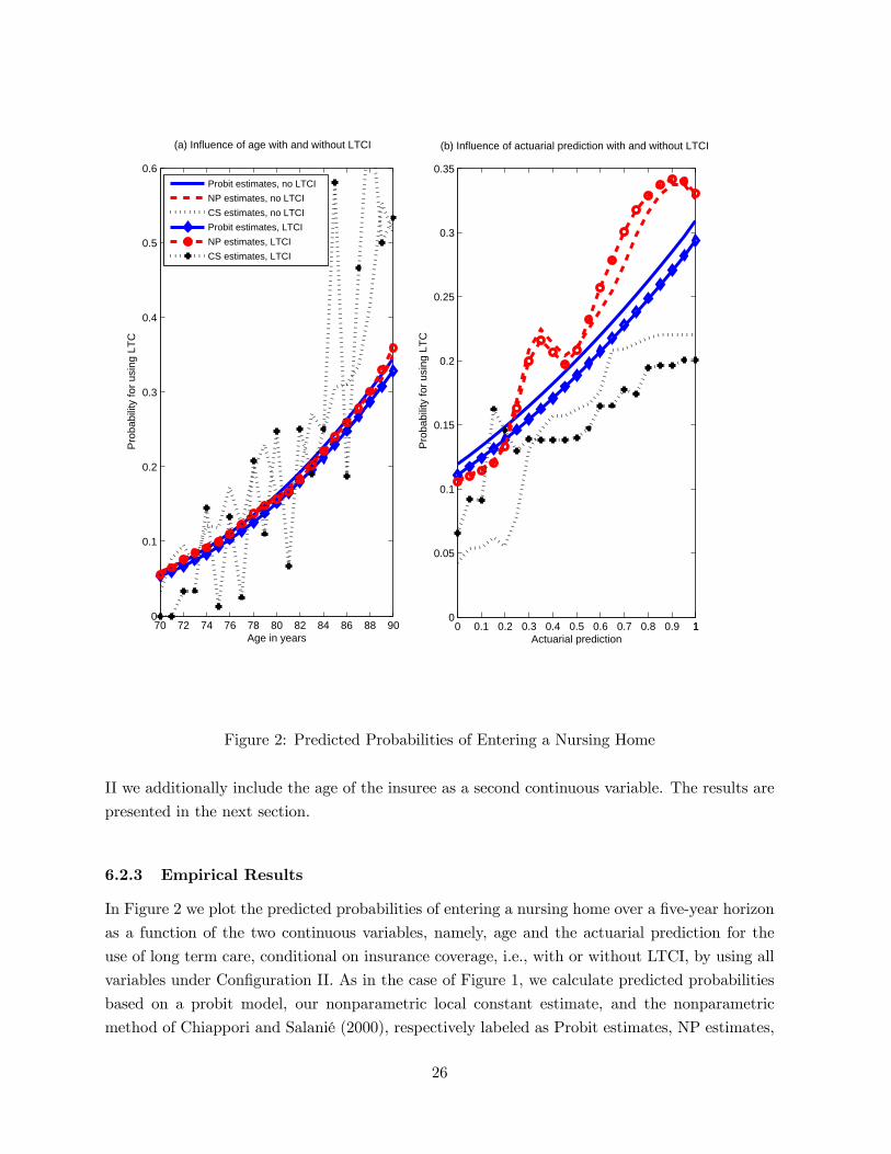
In Figure 2 we plot the predicted probabilities of entering a nursing home over a five-year horizon
as a function of the two continuous variables, namely, age and the actuarial prediction for the
use of long term care, conditional on insurance coverage, i.e., with or without LTCI, by using all
variables under Configuration II. As in the case of Figure 1, we calculate predicted probabilities
based on a probit model, our nonparametric local constant estimate, and the nonparametric
method of Chiappori and Salanié (2000), respectively labeled as Probit estimates, NP estimates,
26

and CS estimates in Figure 2. In order to calculate the CS’s predicted probabilities as a function
of actuarial prediction that takes values between 0 and 1, we use a grid from 0 to 1 with step size
0.05 (with 21 points in total) to discretize the actuarial prediction. To appreciate the differences
between the curves for individuals with and without LTCI, we follow the kind advice of a referee
and lay the curves in the same plane.
We summarize some important findings from Figure 2. First, it shows that the probit model
predicts a monotonic relationship between the predicted (aggregate) probabilities and age (resp.
actuarial prediction) no matter whether an individual has LTCI or not, but our nonparametric
estimates indicate the relationship between the predicted probabilities and age is monotonic but
the predicted probabilities may depend on the actuarial prediction non-monotonically. Second, as
expected, the predicted probabilities based on the CS’s method are not a smooth function of age
due to the transformation of all variables into binary variables and the fact that only information
for a certain age of individuals is used when we calculate the predicted probabilities for that age
group. But the predicted probabilities are a relatively smoother function of actuarial predication
because we only use 21 points to discretize the latter. In any case, the CS’s predictions are quite
different from ours and those based on the probit model. Third, Figure 2(a) suggests that, both
Probit and our NP methods yield similar estimates of the effects of age on the probability of
entering a nursing home for the two groups of senior people with or without LTCI. Based on the
Probit estimates, individuals with LTCI have lower probability of entering a nursing home than
those without LTCI. But our NP estimates suggest that it is difficult to distinguish the estimated
effects of age on the probability of entering a nursing home for individuals with or without LTCI.
Fourth, Figure 2(b) suggests that our NP estimates are significantly different from the Probit
estimates in terms of the effect of actuarial prediction on the probability of entering a nursing
home. The Probit estimates of the effects of actuarial prediction on the probability of entering
a nursing home are always higher for individuals without LTCI than for individuals with LTCI
regardless the level of actuarial prediction. But this is not the case for our NP estimates. Fifth, our
NP estimates reveal that the probability of entering a nursing home is lower for individuals with
LTCI than those without LTCI when both have relatively low actuarial predictions (02 − 05),and the probability of entering a nursing home is higher for those those with LTCI than those
without LTCI when both have relatively high actuarial predictions (05 − 1). Interestingly, forextremely low actuarial predictions (0− 02) the probabilities of entering a nursing home hardlydiffer for individuals with and without LTCI. In sum, we think our findings suggest some sort of
asymmetric information that is related to risk preferences as opposed to risk types and thus lend
support to Finkelstein and McGarry (2006).
For the two configurations described above, Table 6 reports the bootstrap -values for our
nonparametric test based on 500 bootstrap resamples. For either configuration, we can reject the
null hypothesis at the 10% significance level. Therefore we conclude that there is some evidence
of asymmetric information in the long-term care insurance market despite the fact that it is
not overwhelmingly strong. The choice of contract contains information about the occurrence
27

Table 6: Bootstrap p values for our nonparametric test for the long term care insurance
Configurations I II
value 0060 0082
of an accident. This result indicates that a functional and distributional specification is a very
important issue in this field and that probit models might be inappropriate. In order to find some
evidence for asymmetric information in the US long-term care insurance market, Finkelstein and
McGarry (2006) have to resort to the so-called “unused observable”. Our test works without the
need to use such additional information which is only available in some exceptional cases.
7 Concluding Remarks
We propose a new nonparametric test for asymmetric information in this paper and apply it to
a French automobile insurance data set consisting of novice drivers and to the US long term care
insurance market. Our main conclusion for the car insurance data set is that we cannot detect
asymmetric information in the data set despite different configurations of the control variables.
Our nonparametric test does not require specification of any functional or distributional form
among the sets of variables of interest and it is not subject to any misspecification problem given
the right choice of control variables. We also show that excessive bundling does not necessarily
result in a disguise of asymmetric information. Both in the case of the binary choice between
“compulsory” coverage and “additional” coverage and in the case of several deductibles (three
and more groups) we confirm the absence of asymmetric information for young driver in the
French car insurance. Our results are also very strong in contrast to Kim et al. (2009).
Our second application is the US long term care insurance market. While Finkelstein and
McGarry (2006) find no positive correlation between risk and coverage — conditional on the
variables used for risk classification — our test rejects the null hypothesis at the 10% significance
level and therefore we detect the existence of asymmetric information in this market. Whereas
Finkelstein and McGarry (2006) have to use additional information to establish their result, our
test does not require additional information so that the test is widely applicable in most situations.
Our analysis reveals also that a correct functional and distributional specification in this field is
a very important issue and the use of probit models might be inappropriate. This application
shows that our test may have power when other tests do not have.
Since nearly all other classes of insurance, such as the legal protection insurance, private health
insurance, and disability insurance, are structured in the same way as the auto insurance or long
term care insurance, applications to data sets in these subfields are immediate and might help to
gain new insights. Moreover, our test can be applied to more general settings, either to testing
for asymmetric information in other fields or more generally, to testing the general hypothesis of
conditional independence.
28

Mathematical Appendix
A Proof of the Main Results
Let B () ≡ { ( )1 [ (| )− (| )]} ( ) and V () ≡ −1
P=1
( )1 [1 ( ≤ )− (| )] ( ) The following lemma establishes the uniform con-
sistency of b (| ) Lemma A.1 Suppose Assumptions A1-A5 hold. Then uniformly in ( ) ∈ X × Y × Z we
have: b (| ) − (| ) = B () + V () + ((1 + 2)2) = (1 + 2) where
1 ≡ −12 (!)−12√log and 2 ≡ kk2 + kk
Proof. Write b (| ) = b (| ) b ( ) where b (| ) = 1
P=1 ( )1
1 ( ≤ )
and b ( ) = 1
P=1 ( )1
Then we have
b (| )− (| ) =b (| )− b ( ) (| )
( )
"1 +
( )− b ( )b ( )#
= 1 (| ) +2 (| )
where 1 (| ) = [b (| )− b ( ) (| )] ( ) and 2 (| ) = [b (| )− b ( )× (| )][ ( ) − b ( )][ b ( ) ( )] By Theorems 2, 7 and 8 in Hansen (2008) withlittle modification to account for discrete regressors, we can readily show that 2 (| ) = ((1 + 2)
2) uniformly in ( ) ∈ X × Y For 1 (| ) we have
1 (| ) =1
( )
X=1
( )1 [1 ( ≤ )− (| )]
= V () +B () +R ()
where R () = −1P
=1{ ( )1 [ (| )− (| )] − B () ( )} ( )
By the same theorems, we can show that V () = (1) B () = (2) and R () =
(12) uniformly in ( ) ∈ X ×Y. It follows that b (| ) − (| ) = B ()+V ()
+ ((1+2)2) = (1+2) uniformly in ( ) ∈ X ×Y. By the same argument as used
in the proof of Theorem 4.1 of Boente and Fraiman (1991), we can show the above results also
hold uniformly in ∈ Z under Assumption A3. Then the conclusion follows.
Remark. Following Li and Racine (2008), we can write B () =P
=1 21 (| ) +P
=1 2 (| )+smaller order term, where1 (| ) ≡ 12
R2 () [2 (| ) ( )+
( ) (| )] ( ) 2 (| ) ≡P∈X
¡e ¢ [ ¡| e ¢ ¡ e ¢− (| ) ( )] ( ) ( ) ≡
¡
¢ (| ) ≡
¡| ¢ , (| )
≡ 2¡| ¢ ()2 and
¡e ¢ = 1 ¡ 6= e¢Π=1 6=1 ¡ = e¢ Proof of Theorems 4.1 and 4.2
We only prove Theorem 4.2, as the proof of Theorem 4.1 is a special case.
29

First, we observe that (!)12 = (!)12P−2
=0
P−1=+1
P=1[
b (| )− b (| )]2
= 1 +2 + 23 where ≡ ( )
1 ≡ (!)12−2X=0
−1X=+1
X=1
£ (| )− (| )
¤2
2 ≡ (!)12−2X=0
−1X=+1
X=1
h b (| )− (| )− b (| ) + (| )i2 and
3 = (!)12−2X=0
−1X=+1
X=1
[ (| )− (| )]
×h b (| )− (| )− b (| ) + (| )
i
Under H1(−12 (!)−14) we prove the theorem by showing that () 1→ 0 () 2−0
→¡0 20
¢ () 3 = (1) () b = 0 + (1) and () b2 = 20 + (1). For (),
1 = −1P−2
=0
P−1=+1
P=1 ()
2 = 0 + (1) under H1(−12 (!)−14) It remains to
show ()-().
To show (), we first apply Lemma A.1 to obtain
2 = (!)12−2X=0
−1X=+1
X=1
©[V ( )−V ()] + [B ()−B ( )] + (
21 + 22)
ª2
= (!)12−2X=0
−1X=+1
X=1
[V ( )−V ( )]2
+ 2 (!)12−2X=0
−1X=+1
X=1
[V ()−V ()] [B ()−B ()]
+(!)12X=1
[B ()−B ( )]2 + (!)12 (
31 + 32)
≡ 21 + 222 +23 + (1) (A.1)
where the definitions of 21 22 and 23 are self-evident. Let ¡
¢ ≡ ( )1
× [1 ( ≤ )− (| )] ( ) and ¡
¢ ≡ ¡
¢ − ¡
¢ Noting that
V () = −1P
=1 ¡
¢and V ( ) −V ( ) = −1
P=1
¡
¢, we have 21 =
(!)12
2
P=1
P−2=0
P−1=+1[
P=1
¡
¢]2 = + + where ≡ (!)12
2
P=1
P 6=P
6=P−2
=0
P−1=+1
¡
¢ ( ) ≡ (!)12
2
P=1
P=1
P−2=0
P−1=+1
¡
¢2× and ≡ 2(!)12
2
P=1
P 6=P−2
=0
P−1=+1
¡
¢ ( ) Let
¡
¢ ≡[
¡
¢ ( ) +
¡
¢
¡
¢ + ( )
¡
¢] 3 Then
=6 (!)12
2
X1≤≤
−2X=0
−1X=+1
¡
¢=(− 1) (− 2)
30

where ≡ 6(!)12
(−1)(−2)P1≤≤
P−2=0
P−1=+1
¡
¢ Note that for all 6= 6=
≡ £
¡
¢¤= 0 1 () ≡
£
¡
¢¤= 0 and 2(
e) ≡ [(e )] =
13[ ( ) (
e)] Let 3(e ) ≡ (e ) − 2(
e) − 2( ) − 2(e ) By
the Hoeffding decomposition,
= 3(2) +(3)
where (2) ≡ 2(!)12
(−1)P1≤≤
P−2=0
P−1=+1 2
¡
¢and
(3) ≡ 6(!)12
(−1)(−2)P1≤≤P−2
=0
P−1=+1 3( ) Noting that
£3 (e )¤ = 0 and that 3 is symmetric in
its arguments by construction, it is straightforward to show that [(3) ] = 0 and [
(3) ]2 =
(−3 (!)−1) Hence, (3) = (
−32 (!)−12) = ¡−1
¢by the Chebyshev inequality. It
follows that =(−2)−1 = {1 + (1)}H + (1) where
H ≡ 2 (!)12
X1≤≤
−2X=0
−1X=+1
32¡
¢=
2 (!)12
X1≤≤
−2X=0
−1X=+1
Z ( )
¡
¢ () ()
As H is a second order degenerate -statistic, it is straightforward but tedious to verify that all
the conditions of Theorem 1 of Hall (1984) are satisfied, implying that a central limit theorem ap-
plies to H : H→
¡0 lim→∞ 2
¢ where 2 ≡ 2! [
P−2=0
P−1=+1
R ( )
¡
¢× () ()]2 = 2!{
P−2=0
P−1=+1
R[ ( )− ( )]
£
¡
¢− ¡
¢¤ ()
()}2 where denotes expectation with respect to We now show that lim→∞ 2 = 20which is defined in (4.9). In view of the fact that ( ) ( ) = 0 for any 6= we have
2 = 2!
⎧⎨⎩−2X=0
−1X=+1
Z[ ( )
¡
¢+ ( )
¡
¢] () ()
⎫⎬⎭2
= 2!
⎧⎨⎩−2X=0
−1X=+1
( )
⎫⎬⎭2
+ 2!
⎧⎨⎩−2X=0
−1X=+1
( )
⎫⎬⎭2
+4!
⎡⎣−2X=0
−1X=+1
( )
−2X=0
−1X=+1
( )
⎤⎦≡ 21 + 22 + 23 say,
where ( ) ≡R ( )
¡
¢ () () By straightforward but tedious calcula-
tions, one can verify that 21 = 22P−2
=0 ( − 1− )2 + (1) 22 = 22P−1
=1 2+ (1)
and 23 = 42P−2
=1 ( − 1− ) + (1) where =P
∈X
R R R ( )−2 ( ; )2 ()
(|) (|) ()2 It follows that 2 = 22 ( − 1)2P−2
=0 + (1) = 20+ (1) Con-
sequently →
¡0 20
¢ By moment calculations, the Chebyshev inequality, and Assumptions
31
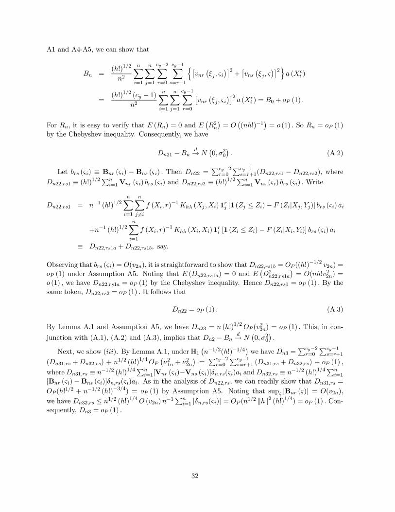
A1 and A4-A5, we can show that
=(!)12
2
X=1
X=1
−2X=0
−1X=+1
n£
¡
¢¤2+£
¡
¢¤2o (
)
=(!)12 ( − 1)
2
X=1
X=1
−1X=0
£
¡
¢¤2 (
) = 0 + (1)
For it is easy to verify that () = 0 and ¡2¢=
¡(!)−1
¢= (1) So = (1)
by the Chebyshev inequality. Consequently, we have
21 −→
¡0 20
¢ (A.2)
Let () ≡ B () − B ( ) Then 22 =P−2
=0
P−1=+1(221 − 222) where
221 ≡ (!)12P
=1V ( ) ( ) and 222 ≡ (!)12P
=1V () () Write
221 = −1 (!)12X=1
X 6=
( )−1 ( )1
[1 ( ≤ )− (| )] ( )
+−1 (!)12X=1
( )−1 ()1
[1 ( ≤ )− (| )] ( )
≡ 221 +221 say.
Observing that ( ) = (2) it is straightforward to show that221 = ((!)−12 2) =
(1) under Assumption A5. Noting that (221) = 0 and ¡2221
¢= (!22) =
(1) we have 221 = (1) by the Chebyshev inequality. Hence 221 = (1) By the
same token, 222 = (1) It follows that
22 = (1) (A.3)
By Lemma A.1 and Assumption A5, we have 23 = (!)12 (22) = (1) This, in con-
junction with (A.1), (A.2) and (A.3), implies that 2 −→
¡0 20
¢
Next, we show (). By Lemma A.1, under H1¡−12(!)−14
¢we have 3 =
P−2=0
P−1=+1
(31 +32) + 12 (!)14
¡21 + 22
¢=P−2
=0
P−1=+1 (31 +32) + (1)
where31 ≡ −12 (!)14P
=1[V ( )−V ( )]() and32 ≡ −12 (!)14P
=1
[B ()−B ()]( ). As in the analysis of 22 we can readily show that 31 =
(!12 + −12 (!)−34) = (1) by Assumption A5. Noting that sup |B ()| = (2),
we have 32 ≤ 12 (!)14 (2)−1P
=1 |()| = (12 kk2 (!)14) = (1) Con-
sequently, 3 = (1)
32

We now show (). Let 1 ≡ 1 (!)−12 ( − 1) Then we have
b −0 =1
X=1
−1X=0
h b ( )−1 b2 (| )− ( )
−1 2 (| )i (
)
+1
X=1
−1X=0
n ( )
−1 2 (| ) ( )−[ ( )
−1 2 (| ) ( )]o
≡ 1 +2 say.
By the Chebyshev inequality, it is straightforward to show that 2 = ((!)−12) = (1)
Use the fact that b ( )− ( ) = (1 + 2) and b2 (| )−2 (| ) = (1 + 2)
uniformly in ( ) ∈ X×Y×Z, we can readily show that 1 = (!)−12 (1 + 2) = (1)
under Assumption A5. Consequently, b −0 = (1)
For (), letting 2 ≡ 22 ( − 1)2 we have
b2 − 20
=2
(− 1)X=1
X 6=
−1X=0
hb ( )− ( )i (
)
¡
¢+
2
(− 1)X=1
X 6=
−1X=0
© ( ) (
)
¡
¢−£ ( ) (
)
¡
¢¤ª+
1
(− 1)X=1
X 6=
⎧⎨⎩2
−1X=0
£ ( ) (
)
¡
¢¤− 20
⎫⎬⎭≡ 1 + 2 + 3 say,
where ( ) = ( )−1 ( )
−1 ( ; ) ( ; ) and b ( ) = b ( )−1b ( )
−1 b ( ; )b ( ; ) Using the uniform consistency of b ( ) and b (| ) we can readily show that 1 = (1 + 2) = (1) By the law of large numbers for second
order -statistic, 2 = (1) By moment calculations, 3 = (2) = (1) Thus we haveb2 = 20 + (1). ¥Proof of Theorems 4.3
Using the notation defined in the proof of Theorem 4.2, we have −1 = −1 (!)−12 (1+
2+23) Under H1, it is easy to show that −1 (!)−121 =P−2
=0
P−1=+1 [ (| )
− (| )]2 + (1)
−1 (!)−122 = (21 + 22) = (1) and −1 (!)−123 =
(1 + 2) = (1) On the other hand, −1 (!)−12 b =
¡−1
¢= (1) and b2 =
20 + (1). It follows that −1 (!)−12 = (−1− −1 (!)−12 b)
qb2 →P−2=0
P−1=+1
[ (| )− (| )]20 and the conclusion follows. ¥
ACKNOWLEDGMENTS
The authors sincerely thank Keisuke Hirano, the associate editor, and three anonymous refer-
ees for their many insightful comments and suggestions that lead to a substantial improvement of
33

the presentation. They are very grateful to Bernard Salanié for his most valuable comments and
for providing us with the first data set used in the paper. They gratefully acknowledge a referee
for pointing to them that Dionne, Gourieroux, and Vanasse (2001, 2006) first formulate the test
of asymmetric information as a test of conditional independence as outlined in Section 3.1. Spind-
ler gratefully acknowledges financial support from the Deutsche Forschungsgemeinschaft through
GRK 801.
References
Aitchison, J., and Aitken, C. G. G. (1976), “Multivariate Binary Discrimination by the KernelMethod,” Biometrika 63, 413-420.
Akerlof, G. (1970), “The Market for Lemons: Quality Uncertainty and the Market Mechanism,”Quarterly Journal of Economics 84, 488-500.
Boente, G., and Fraiman, R. (1991), “Strong Uniform Convergence Rates for Some RobustEquivariant Nonparametric Regression Estimates for Mixing Processes,” International Stat-istical Review 59, 355-372.
Chiappori, P.-A., and Heckman, J. J. (1999), “Testing for Moral Hazard Using Dynamic Data,”Manuscript, Dept. of Economics, University of Chicago.
Chiappori, P.-A., and Salanié, B. (1997), “Empirical Contract Theory: the Case of InsuranceData,” European Economic Review 41, 943-950.
Chiappori, P.-A., and Salanié, B. (2000), “Testing for Asymmetric Information in InsuranceMarkets,” Journal of Political Economy 108, 56-78.
Chiappori, P.-A., Jullien, B., Salanié, B., and Salanié, F. (2006), “Asymmetric Information inInsurance: General Testable Implications,” Rand Journal of Economics 37, 783-798.
Cohen, A. (2005), “Asymmetric Information and Learning: Evidence from the AutomobileInsurance Market,” Review of Economics and Statistics 87, 197-207.
Cohen, A., and Siegelman, P. (2010), “Testing for Adverse Selection in Insurance Markets,”Journal of Risk and Insurance 77, 39-84.
Crocker, K.-J., and Snow, A. (2000), “The Theory of Risk Classification,” in Handbook of In-surance, eds., G. Dionne, pp. 245-276. Kluwer Academic Publishers.
De Jong, P. and Heller, G. Z. (2008), Generalized Linear Models for Insurance Data, Oxford:Oxford University Press.
Delgado, M. A., and González-Manteiga, W. (2001), “Significance Testing in NonparametricRegression Based on the Bootstrap,” Annals of Statistics 29, 1469-1507.
Dionne, G., Doherty, N., and Fombaron, N. (2000), “Adverse Selection in Insurance Markets,”in Handbook of Insurance, eds. G. Dionne, pp. 185-244. Kluwer Academic Publishers.
Dionne, G., Gourieroux C., and Vanasse, C. (2001), “Testing for Evidence of Adverse Selectionin the Automobile Insurance Market: A Comment,” The Journal of Political Economy 109,444-453.
Dionne, G., Gourieroux, C., and Vanasse, C., (2006), “Informational Content of HouseholdDecisions with Applications to Insurance under Asymmetric Information,” in Competitivefailures in insurance markets: Theory and policy implications, eds. P. A. Chiappori and C.Gollier, pp. 159-184. Cambridge, MA: MIT Press.
34

Dionne, G., Michaud, P.-C., and Dahchour, M. (2012), “Separating Moral Hazard from AdverseSelection in Automobile Insurance: Longitudinal Evidence from France,” Journal of theEuropean Economic Association forthcoming.
Finkelstein, A., and McGarry, K. (2006), “Multiple Dimensions of Private Information: Evidencefrom the Long-term Care Insurance Market,” American Economic Review 96, 938-958.
Finkelstein, A., and Poterba, J. (2006), “Testing for Adverse Selection with ‘Unused Observ-ables’,” NBER Working Paper 12112.
Gan, L., Huang, F., and Mayer, A. (2011), “A Simple Test of Private Information in the Insur-ance Markets with Heterogeneous Insurance Demand,” NBER Working Paper 16738.
Gourieroux, C., Monfort, A., Renault, E., and Trognon, A. (1987), “Generalised Residuals,”Journal of Econometrics 34, 5-32.
Hall, P. (1984), “Central Limit Theorem for Integrated Square Error of Multivariate Nonpara-metric Density Estimators,” Journal of Multivariate Analysis 14, 1-16.
Hansen, B. E. (2008), “Uniform Convergence Rates for Kernel Estimation with DependentData,” Econometric Theory 24, 726-748.
Horowitz, J. L., and Spokoiny, V. G. (2001), “An Adaptive, Rate-optimal Test of a ParametricMean-regression Model against a Nonparametric Alternative,” Econometrica, 69, 599-631.
Huang, M., and White, H. (2009), “A flexible Test for Conditional Independence,” WorkingPaper, Dept. of Economics, UCSD.
Huang, T.-M. (2010), “Testing Conditional Independence Using Maximal Nonlinear ConditionalIndependence,” Annals of Statistics, 38, 2047-2091.
Jullien, B., Salanié, B., and Salanié, F. (2007), “Screening Risk Averse Agents under MoralHazard,” Economic Theory 30, 151-169.
Kaas, R., Goovaerts, M., Dhaene, J., and Denuit, M. (2008), Modern Actuarial Risk Theory:Using R, Springer, 2nd edition.
Kim, H., Kim, D., Im, S., and Hardin, J. W. (2009), “Evidence of Asymmetric Informationin the Automobile Insurance Market: Dichotomous versus Multinomial Measurement ofInsurance Coverage,” Journal of Risk and Insurance 76, 343-366.
Li, Q., and Racine, J. (2007), Nonparametric Econometrics: Theory and Practice. Princeton:Princeton University Press.
Li, Q., and Racine, J. (2008), “Nonparametric Estimation of Conditional CDF and QuantileFunctions with Mixed Categorical and Continuous Data,” Journal of Business and Eco-nomic Statistics 26, 423-434.
Mikosch, T. (2006), Non-Life Insurance Mathematics: An Introduction with Stochastic Processes.Springer.
Paparoditis, E., and Politis, D. N. (2000), “The Local Bootstrap for Kernel Estimators underGeneral Dependence Conditions,” Annals of the Institute of Statistical Mathematics 52,139-159.
Puelz, R., and Snow, A. (1994), “Evidence on Adverse Selection: Equilibrium Signaling andCross-subsidization in the Insurance Market,” Journal of Political Economy 102, 236-257.
Racine, J., and Li, Q. (2004), “Nonparametric Estimation of Regression Functions with BothCategorical and Continuous Data,” Journal of Econometrics 119, 99-130.
35

Richaudeau, D. (1999), “Automobile Insurance Contracts and Risk of Accident: an EmpiricalTest Using French Individual Data,” The Geneva Papers on Risk and Insurance Theory 24,97-114.
Robinson, J. (1996), “A Long-term Care Status Transition Model,” presented at Bowles Sym-posium on the Old-Age Crisis: Actuarial Opportunities, Georgia State University, Septem-ber 26-27, 1996.
Rothschild, M., and Stiglitz, J. E. (1976) “Equilibrium in Competitive Insurance Markets: AnEssay on the Economics of Imperfect Information,” Quarterly Journal of Economics 90,630-649.
Saito, K. (2009), “Testing for Asymmetric Information in the Automobile Insurance Marketunder Rate Regulation,” The Journal of Risk and Insurance 73, 335-356.
Song, K. (2009), “Testing Conditional Independence via Rosenblatt Transform,” Annals of Stat-istics 37, 4011-4045.
Su, L., and Ullah, A. (2009), “Testing Conditional Uncorrelatedness,” Journal of Business andEconomic Statistics, 27, 18-29.
Su, L., and White, H. (2007), “A Consistent Characteristic-function-based Test for ConditionalIndependence,” Journal of Econometrics 141, 807-834.
Su, L., and White, H. (2008), “A Nonparametric Hellinger Metric Test for Conditional Inde-pendence,” Econometric Theory 24, 829-864.
Winter, R. (2000), “Optimal Insurance under Moral Hazard,” in Handbook of Insurance, eds.G. Dionne, pp.155-184. Kluwer Academic Publishers.
36