Nonparametric Blind Super-Resolution

Tomer Michaeli and Michal IraniDept. of Computer Science and Applied Mathematics

Weizmann Institute of Science, Israel

Abstract

Super resolution (SR) algorithms typically assume that

the blur kernel is known (either the Point Spread Function

‘PSF’ of the camera, or some default low-pass filter, e.g. a

Gaussian). However, the performance of SR methods sig-

nificantly deteriorates when the assumed blur kernel devi-

ates from the true one. We propose a general framework

for “blind” super resolution. In particular, we show that:

(i) Unlike the common belief, the PSF of the camera is the

wrong blur kernel to use in SR algorithms. (ii) We show how

the correct SR blur kernel can be recovered directly from

the low-resolution image. This is done by exploiting the in-

herent recurrence property of small natural image patches

(either internally within the same image, or externally in a

collection of other natural images). In particular, we show

that recurrence of small patches across scales of the low-res

image (which forms the basis for single-image SR), can also

be used for estimating the optimal blur kernel. This leads to

significant improvement in SR results.

1. Introduction

Super-resolution (SR) refers to the task of recovering

a high-resolution image from one or several of its low-

resolution versions. Most SR methods (e.g. [11, 7, 2, 4, 20,

16, 15, 21]) assume that the low-resolution input image was

obtained by down-sampling the unknown high-resolution

image with a known blur kernel. This is usually assumed

to be the Point Spread Function (PSF) of the camera. When

the PSF is unknown, the blur kernel is assumed to be some

standard low-pass filter (LPF) like a Gaussian or a bicubic

kernel. However, the PSF may vary in practice with zoom,

focus, and/or camera shake. Relying on the wrong blur ker-

nel may lead to low-quality SR results, as demonstrated in

Fig. 1. Moreover, we show that unlike the common belief,

even if the PSF is known, it is the wrong blur kernel to use in

SR algorithms! We further show how to obtain the optimal

SR blur kernel directly from the low-resolution image.

A very limited amount of work has been dedicated to

“blind SR”, namely SR in which the blur kernel is not as-

sumed known. Most methods in this category assume some

parametric model for the kernel (e.g. still a Gaussian, but

with unknown width) and infer its parameters [17, 1, 19].

Extension to multiple parametric models appears in [10].

A nonparametric kernel recovery method was presented in

Low-resolution image Default kernel Recovered kernel

SR of [8] with its default kernel SR of [8] with our recovered kernel

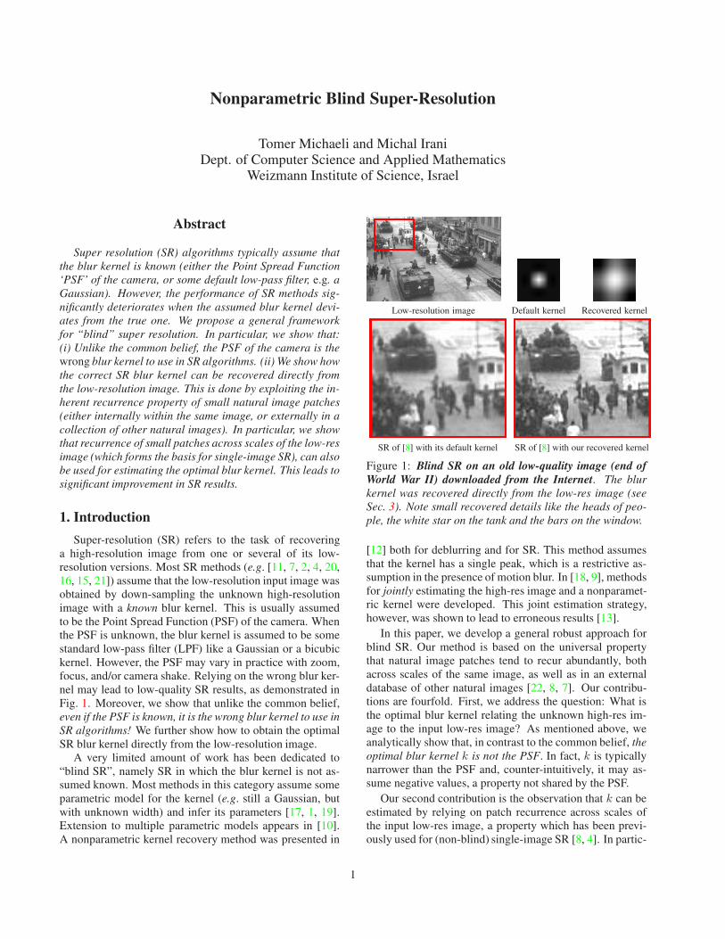
Figure 1: Blind SR on an old low-quality image (end of

World War II) downloaded from the Internet. The blur

kernel was recovered directly from the low-res image (see

Sec. 3). Note small recovered details like the heads of peo-

ple, the white star on the tank and the bars on the window.

[12] both for deblurring and for SR. This method assumes

that the kernel has a single peak, which is a restrictive as-

sumption in the presence of motion blur. In [18, 9], methods

for jointly estimating the high-res image and a nonparamet-

ric kernel were developed. This joint estimation strategy,

however, was shown to lead to erroneous results [13].

In this paper, we develop a general robust approach for

blind SR. Our method is based on the universal property

that natural image patches tend to recur abundantly, both

across scales of the same image, as well as in an external

database of other natural images [22, 8, 7]. Our contribu-

tions are fourfold. First, we address the question: What is

the optimal blur kernel relating the unknown high-res im-

age to the input low-res image? As mentioned above, we

analytically show that, in contrast to the common belief, the

optimal blur kernel k is not the PSF. In fact, k is typically

narrower than the PSF and, counter-intuitively, it may as-

sume negative values, a property not shared by the PSF.

Our second contribution is the observation that k can be

estimated by relying on patch recurrence across scales of

the input low-res image, a property which has been previ-

ously used for (non-blind) single-image SR [8, 4]. In partic-

1

ular, we show that the kernel that maximizes the similarity

of recurring patches across scales of the low-res image, is

also the optimal SR kernel. Based on this observation, we

propose an iterative algorithm for recovering the kernel.

Many example-based SR algorithms rely on an external

database of low-res and high-res pairs of patches extracted

from a large collection of high-quality example images [20,

21, 7, 2]. They too assume that the blur kernel k is known

a-priori (and use it to generate the low-res versions of the

high-res examples). We show how our kernel estimation

algorithm can be modified to work with an external database

of images, recovering the optimal kernel relating the low-res

image to the external high-res examples.

Our last contribution is a proof that our algorithm com-

putes the MAP estimate of the kernel, as opposed to the

joint MAP (over the kernel and high-res image) strategy of

[19, 10, 18, 9]. The benefit of this approach has been studied

and demonstrated in the context of blind deblurring [13].

We show that plugging our estimated kernel into existing

super-resolution algorithms results in improved reconstruc-

tions that are comparable to using the ground-truth kernel.

2. What is the correct SR kernel?

Let l denote a low-resolution image. Super-resolution

can be viewed as trying to recover a high-resolution image

h of the same scene, as if taken by the same camera, but

with an optical zoom-in by a factor of α. This allows to

view fine details, that are smaller than a pixel size in l.The low-res image l is generated from a continuous-

space image f and a continuous-space PSF bL, as1

l[n] =

∫

f(x)bL(n− x)dx. (1)

The unknown high-res image h corresponds to a finer grid,

h[n] =

∫

f(x)bH

(n

α− x)

dx, (2)

where bH is the high-res PSF. E.g., in the case of optical

zoom, bH is a narrower (scaled-down) version of bL, namely

bH(x) = αbL(αx). (3)

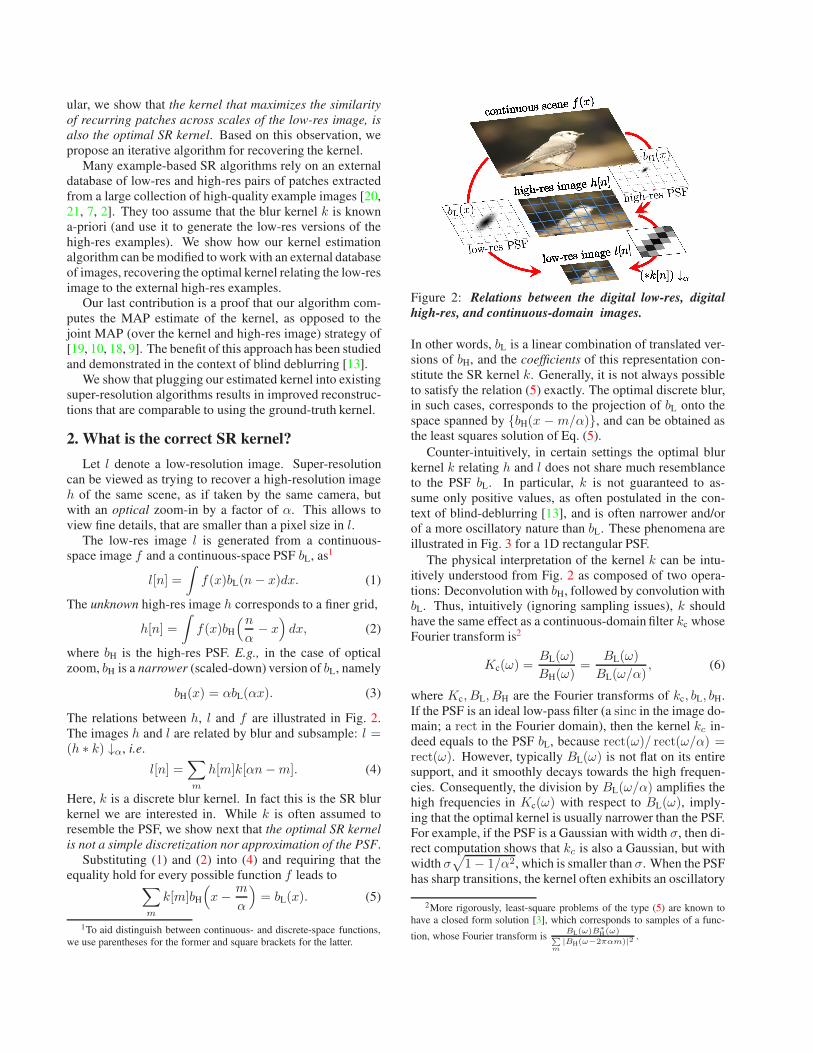
The relations between h, l and f are illustrated in Fig. 2.

The images h and l are related by blur and subsample: l =(h ∗ k) ↓α, i.e.

l[n] =∑

m

h[m]k[αn−m]. (4)

Here, k is a discrete blur kernel. In fact this is the SR blur

kernel we are interested in. While k is often assumed to

resemble the PSF, we show next that the optimal SR kernel

is not a simple discretization nor approximation of the PSF.

Substituting (1) and (2) into (4) and requiring that the

equality hold for every possible function f leads to∑

m

k[m]bH

(

x−m

α

)

= bL(x). (5)

1To aid distinguish between continuous- and discrete-space functions,

we use parentheses for the former and square brackets for the latter.

Figure 2: Relations between the digital low-res, digital

high-res, and continuous-domain images.

In other words, bL is a linear combination of translated ver-

sions of bH, and the coefficients of this representation con-

stitute the SR kernel k. Generally, it is not always possible

to satisfy the relation (5) exactly. The optimal discrete blur,

in such cases, corresponds to the projection of bL onto the

space spanned by {bH(x −m/α)}, and can be obtained as

the least squares solution of Eq. (5).

Counter-intuitively, in certain settings the optimal blur

kernel k relating h and l does not share much resemblance

to the PSF bL. In particular, k is not guaranteed to as-

sume only positive values, as often postulated in the con-

text of blind-deblurring [13], and is often narrower and/or

of a more oscillatory nature than bL. These phenomena are

illustrated in Fig. 3 for a 1D rectangular PSF.

The physical interpretation of the kernel k can be intu-

itively understood from Fig. 2 as composed of two opera-

tions: Deconvolution with bH, followed by convolution with

bL. Thus, intuitively (ignoring sampling issues), k should

have the same effect as a continuous-domain filter kc whose

Fourier transform is2

Kc(ω) =BL(ω)

BH(ω)=

BL(ω)

BL(ω/α), (6)

where Kc, BL, BH are the Fourier transforms of kc, bL, bH.

If the PSF is an ideal low-pass filter (a sinc in the image do-

main; a rect in the Fourier domain), then the kernel kc in-

deed equals to the PSF bL, because rect(ω)/ rect(ω/α) =rect(ω). However, typically BL(ω) is not flat on its entire

support, and it smoothly decays towards the high frequen-

cies. Consequently, the division by BL(ω/α) amplifies the

high frequencies in Kc(ω) with respect to BL(ω), imply-

ing that the optimal kernel is usually narrower than the PSF.

For example, if the PSF is a Gaussian with width σ, then di-

rect computation shows that kc is also a Gaussian, but with

width σ√

1− 1/α2, which is smaller than σ. When the PSF

has sharp transitions, the kernel often exhibits an oscillatory

2More rigorously, least-square problems of the type (5) are known to

have a closed form solution [3], which corresponds to samples of a func-

tion, whose Fourier transform isBL(ω)B∗

H(ω)∑

m|BH(ω−2παm)|2

.

bL(x)knaive[n]

Discretization of the PSF

koptimal[n]

Optimal blur k computed from (5)

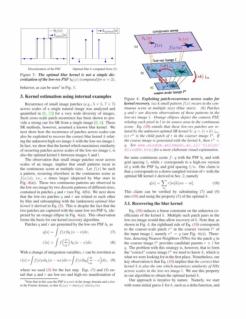
Figure 3: The optimal blur kernel is not a simple dis-

cretization of the low-res PSF bL(x) (computed for α = 2).

behavior, as can be seen3 in Fig. 3.

3. Kernel estimation using internal examples

Recurrence of small image patches (e.g., 5 × 5, 7 × 7)

across scales of a single natural image was analyzed and

quantified in [8, 22] for a very wide diversity of images.

Such cross-scale patch recurrence has been shown to pro-

vide a strong cue for SR from a single image [8, 6]. These

SR methods, however, assumed a known blur kernel. We

next show how the recurrence of patches across scales can

also be exploited to recover the correct blur kernel k relat-

ing the unknown high-res image h with the low-res image l.In fact, we show that the kernel which maximizes similarity

of recurring patches across scales of the low-res image l, is

also the optimal kernel k between images h and l.The observation that small image patches recur across

scales of an image, implies that small patterns recur in

the continuous scene at multiple sizes. Let f(x) be such

a pattern, recurring elsewhere in the continuous scene as

f(x/α), i.e., α times larger (depicted by blue stars in

Fig. 4(a)). These two continuous patterns are observed in

the low-res image by two discrete patterns of different sizes,

contained in patches q and r (see Fig. 4(b)). We next show

that the low-res patches q and r are related to each other

by blur and subsampling with the (unknown) optimal blur

kernel k derived in Eq. (5). This is despite the fact that the

two patches are captured with the same low-res PSF bL (de-

picted by an orange ellipse in Fig. 4(a)). This observation

forms the basis for our kernel recovery algorithm.

Patches q and r are generated by the low-res PSF bL as

q[n] =

∫

f(x)bL(n− x)dx, (7)

r[n] =

∫

f(x

α

)

bL(n− x)dx. (8)

With a change of integration variables, r can be rewritten as

r[n]=

∫

f(x)αbL(n− αx)dx=

∫

f(x)bH

(n

α− x)

dx, (9)

where we used (3) for the last step. Eqs. (7) and (9) en-

tail that q and r are low-res and high-res manifestation of

3Note that in this case the PSF is a rect in the image domain and a sincin the Fourier domain, so that Kc(ω) = sinc(ω)/ sinc(ω/α).

Figure 4: Exploiting patch-recurrence across scales for

kernel recovery. (a) A small pattern f(x) recurs in the con-

tinuous scene at multiple sizes (blue stars). (b) Patches

q and r are discrete observations of these patterns in the

low-res image l. Orange ellipses depict the camera PSF,

relating each pixel in l to its source area in the continuous

scene. Eq. (10) entails that these low-res patches are re-

lated by the unknown optimal SR kernel k: q = (r ∗ k) ↓α.

(c) rα is the child patch of r in the coarser image lα. If

the coarse image is generated with the kernel k, then rα =q. See www.wisdom.weizmann.ac.il/˜vision/

BlindSR.html for a more elaborate visual explanation.

the same continuous scene f : q with the PSF bL and with

grid spacing 1, while r corresponds to a high-res version

of q with the PSF bH and grid spacing 1/α. Our claim is

that q corresponds to a down-sampled version of r with the

optimal SR kernel k derived in Sec. 2, namely

q[n] =∑

m

r[m]k[αn−m]. (10)

This claim can be verified by substituting (7) and (9)

into (10) and using the property (5) of the optimal k.

3.1. Recovering the blur kernel

Eq. (10) induces a linear constraint on the unknown co-

efficients of the kernel k. Multiple such patch pairs in the

low-res image would thus allow recovery of k. Note that, as

shown in Fig. 4, the righthand side of Eq. (10) corresponds

to the coarser-scale patch rα in the coarser version lα of

the input image l, namely rα = q (see Fig. 4(c)). There-

fore, detecting Nearest-Neighbors (NNs) for the patch q in

the coarser image lα provides candidate parents r ∈ l for

q. The problem with this strategy is, however, that to form

the “correct” coarse image lα we need to know k, which is

what we were looking for in the first place. Nonetheless, our

key observation is that Eq. (10) implies that the correct blur

kernel k is also the one which maximizes similarity of NNs

across scales in the low-res image l. We use this property

in our algorithm to obtain the optimal kernel k.

Our approach is iterative by nature. Namely, we start

with some initial guess k for k, such as a delta function, and

use it to down-sample l. Next, for each small patch qi in lwe find a few nearest neighbors (NNs) in lα and regard the

large patches right above them as the candidate “parents”

of qi. The so found parent-child pairs (q, r) are then used

to construct a set of linear equations (using (10)), which is

solved using least-squares to obtain an updated k. These

steps are repeated until convergence. Note that the least-

squares step does not recover the initial kernel k we use to

down-sample the image, but rather a kernel that is closer to

the true k. This is because, as our experience shows, even

with an inaccurate kernel, many of the NNs of qi are located

at the same image coordinates in lα as the NNs correspond-

ing to the correct k. Thus, in each iteration the number

of correct NNs increases and the estimate gets closer to k.

As long as the root mean squared error (RMSE) between

patches in l and their NNs in lα keeps decreasing, we keep

iterating. Our experiments show that this process converges

to the correct k very quickly (typically ∼ 15 iterations), and

is insensitive to the choice of initial guess k (see Figs. 6

and 7 in Sec. 6).

Not all patches in l need to recur (have similar patches) in

the coarse image lα in order to be able to recover k. For ex-

ample, recovering a 7×7 discrete kernel k relating high-res

h with low-res l (49 unknowns) may be done with as little

as one good 7×7 patch recurring in scales l and lα (provid-

ing 49 equations). When using multiple patches, the NNs

should intuitively be weighted according to their degree of

similarity to the query patches {qi}, so that good NNs con-

tribute more than their poor counterparts. It may also be de-

sired to add a regularization term to the least-squares prob-

lem solved in each iteration, in order to impose smoothness

constraints on the kernel. We defer the discussion on these

issues to Sec. 5, where we also provide a detailed summary

of the algorithm (see Alg. 1).

Figs. 1,5,9 show examples of single-image SR with the

method of [8], once using their default (bicubic) kernel, and

once using our kernel recovered from the low-res image.

4. Kernel estimation using external examples

Many example-based SR algorithms rely on an external

database of high-res patches extracted from a large collec-

tion of high-res images [20, 21, 7, 2]. They too assume

that the blur kernel k is known a-priori, and use it to down-

sample the images in the database in order to obtain pairs

of low-res and high-res patches. Roughly speaking, these

pairs are used to learn how to “undo” the operation of down-

sampling with k, so that, given an input image l, its cor-

responding high-res version h can be reconstructed. We

first explain the physical interpretation of the optimal ker-

nel k when using an external database of examples, and then

show how to estimate this optimal k.

Let us assume, for simplicity, that all the high-res images

in the external database were taken by a single camera with

a single PSF. Since the external images form examples of

the high-res patches in SR, this implicitly induces that the

high-res PSF bH is the PSF of the external camera. The

external camera, however, is most likely not the same as the

camera imaging the low-res input image l (the “internal”

camera). Thus, the high-res PSF bH and the low-res PSF

bL may not necessarily have the same profile (i.e. one is

no longer a scaled version of the other). It is important to

note that the discussion in Sec. 2 remains valid. Namely

the kernel k relating the high-res and low-res images is still

given by Eqs. (5) and (6) in these settings, but with a PSF

bH of a different camera. According to Eq. (6), the intuitive

understanding of the optimal kernel k when using external

high-res examples is (in the Fourier domain):

Kc(ω) =BL(ω)

BH(ω)=

PSF Internal(ω)

PSFExternal(ω). (11)

Thus, in SR from external examples the high-res patches

correspond to the PSF bH of the external camera, and the

low-res patches generated from them by downsampling

with k should correspond, by construction, to the low-res

PSF bL of the internal camera. This k is generally unknown

(and is assumed by external SR methods to be some default

kernel, like a Guassian, or a bicubic kernel).

Determining the optimal kernel k for external SR can be

done in the same manner as for internal SR (Sec. 3.1), with

the only exception that the “parent” patches {ri} are now

sought in an external database rather than within the input

image. As before, we start with an initial guess k to the ker-

nel k. We down-sample the external patches {ri} with k to

obtain their low-res versions {rαi }. Then each low-res patch

q in the low-res image l searches for its NNs among {rαi },

to find its candidate parents {ri} in the database. These

“parent-child” pairs (q, r) are used to recover a more ac-

curate kernel k via a least-squares solution to a system of

linear equations. This process is repeated until convergence

to the final estimated kernel. Fig. 5 provides an example

of external SR with the algorithm of [21], once using their

default (bicubic) kernel k, and once using our kernel k esti-

mated from their external examples.

5. Interpretation as MAP estimation

We next show that both our approaches to kernel estima-

tion (internal and external) can be viewed as a principled

Maximum a Posteriori (MAP) estimation. Some existing

blind SR approaches attempt to simultaneously estimate the

high-res image h and the kernel k [19, 10, 18, 9]. This is

done by assuming a prior on each of them and maximizing

the posterior probability p(h, k|l). In the context of blind

deblurring, this MAPh,k approach has been shown to lead

to inaccurate estimates of k [13]. This is in contrast to the

MAPk method [5, 13, 14] which seeks to estimate k alone,

by maximizing its marginal posterior, p(k|l). As we show

next, the algorithm presented in Secs. 3 and 4 computes the

MAPk estimate. However, unlike [14], our MAPk is based

on a nonparametric prior.

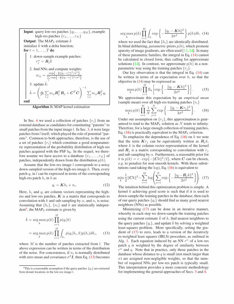
Input: query low-res patches {q1, . . . , qM}, example

high-res patches {r1, . . . , rN}

Output: The MAPk estimate k

initialize k with a delta function;

for t = 1, . . . , T do

1. down-sample example patches:

rαj = Rj k

2. find NNs and compute weights:

wij =exp{− 1

2‖qi−rαj ‖2/σ2}

∑

j

exp{− 1

2‖qi−rα

j‖2/σ2}

3. update k:

k =

(

1σ2

∑

i,j

wijRTj Rj +C

TC

)−1

∑

i,j

wijRTj qi

end

Algorithm 1: MAP kernel estimation

In Sec. 4 we used a collection of patches {ri} from an

external database as candidates for constituting “parents” to

small patches from the input image l. In Sec. 3, it were large

patches from l itself, which played the role of potential “par-

ents”. Common to both approaches, therefore, is the use of

a set of patches {ri} which constitute a good nonparamet-

ric representation of the probability distribution of high-res

patches acquired with the PSF bH. In the sequel, we there-

fore assume we have access to a database {r1, . . . , rN} of

patches, independently drawn from the distribution p(h).Assume that the low-res image l corresponds to a noisy

down-sampled version of the high-res image h. Then, every

patch qi in l can be expressed in terms of the corresponding

high-res patch hi in h as

qi = Khi + ni. (12)

Here, hi and qi are column vectors representing the high-

res and low-res patches, K is a matrix that corresponds to

convolution with k and sub-sampling by α, and ni is noise.

Assuming that {hi}, {ni} and k are statistically indepen-

dent4, the MAPk estimate is given by

k = argmaxk

p(k)

M∏

i=1

p(qi|k)

= argmaxk

p(k)

M∏

i=1

∫

hi

p(qi|hi, k)p(hi)dhi, (13)

where M is the number of patches extracted from l. The

above expression can be written in terms of the distribution

of the noise. For concreteness, if ni is normally distributed

with zero mean and covariance σ2I , then Eq. (13) becomes

4This is a reasonable assumption if the query patches {qi} are extracted

from distant locations in the low-res image l.

argmaxk

p(k)

M∏

i=1

∫

h

exp

{

−‖qi −Kh‖2

2σ2

}

p(h)dh, (14)

where we used the fact that {hi} are identically distributed.

In blind deblurring, parametric priors p(h), which promote

sparsity of image gradients, are often used [13, 14]. In many

of these parametric families, the integral in Eq. (14) cannot

be calculated in closed form, thus calling for approximate

solutions [14]. In contrast, we approximate p(h) in a non-

parametric way using the training patches {rj}.

Our key observation is that the integral in Eq. (14) can

be written in terms of an expectation over h, so that the

objective in (14) may be expressed as

maxk

p(k)

M∏

i=1

Eh

[

exp

{

−‖qi −Kh‖2

2σ2

}]

. (15)

We approximate this expectation by an empirical mean

(sample mean) over all high-res training patches {ri}

maxk

p(k)

M∏

i=1

1

N

N∑

j=1

exp

{

−‖qi −Krj‖

2

2σ2

}

. (16)

Under our assumption on {rj}, this approximation is guar-

anteed to tend to the MAPk solution as N tends to infinity.

Therefore, for a large enough collection of training patches,

Eq. (16) is practically equivalent to the MAPk criterion.

To emphasize the dependence of Eq. (16) on k we note

that the term Krj can be equivalently written as Rjk,

where k is the column-vector representation of the kernel

and Rj is a matrix corresponding to convolution with rjand sub-sampling by α. Furthermore, a reasonable prior for

k is p(k) = c · exp{−‖Ck‖2/2}, where C can be chosen,

e.g. to penalize for non-smooth kernels. With these substi-

tutions (and taking the log), Eq. (16) is equivalent to

mink

1

2‖Ck‖2−

M∑

i=1

log

N∑

j=1

exp

{

−‖qi−Rjk‖

2

2σ2

}

. (17)

The intuition behind this optimization problem is simple. A

kernel k achieving good score is such that if it is used to

down-sample the training patches in the database, then each

of our query patches {qi} should find as many good nearest

neighbors (NNs) as possible.

Minimizing (17) can be done in an iterative manner,

whereby in each step we down-sample the training patches

using the current estimate k of k, find nearest neighbors to

the query patches {qi}, and update k by solving a weighted

least-squares problem. More specifically, setting the gra-

dient of (17) to zero, leads to a version of the iteratively

re-weighted least squares (IRLS) procedure, as outlined in

Alg. 1. Each equation induced by an NN rα of a low-res

patch q is weighted by the degree of similarity between

rα and q. Note that in practice, only those patches in the

database whose distance to q is small (not much larger than

σ) are assigned non-negligible weights, so that the num-

ber of required NNs per low-res patch is typically small.

This interpretation provides a more concrete methodology

for implementing the general approaches of Secs. 3 and 4.

6. Experimental results

We validated the benefit of using our kernel estimation

in SR algorithms both empirically (on low-res images gen-

erated with ground-truth data), as well as visually on real

images. We use the method of [8] as a representative of SR

methods that rely on internal patch recurrence, and the al-

gorithm of [21] as representative of SR methods that train

on an external database of examples.

In our experiments the low-res patches q and rα were

5×5 patches. We experimented with SR×2 and SR×3. We

typically solve for 9 × 9, 11 × 11 or 13 × 13 kernels. The

noise level was assumed to be σ = 10. For the external ker-

nel recovery we used a database of 30 natural images down-

loaded from the Internet (most likely captured by different

cameras). The regularization in the least-squares stage of

each iteration (see Alg. 1) was performed with a matrix C

corresponding to derivatives in the x and y directions.

To quantify the effect of our estimated kernel k on SR

algorithms, we use two measures. The Error Ratio to

Ground Truth (ERGT), which was suggested in the con-

text of blind deblurring [13], measures the ratio between

the SR reconstruction error with our k and the SR recon-

struction error with the ground-truth k, namely ERGT =

‖h− hk‖2/‖h− hk‖

2. Values close to 1 indicate that the es-

timated kernel k is nearly as good as the ground-truthk. The

Error Ratio to Default (ERD) measure quantifies the bene-

fit of using the estimated kernel k over the default (bicubic)

kernel kd, and is defined as ERD = ‖h− hk‖2/‖h− hkd

‖2.

Values much smaller than 1 indicate a large improvement.

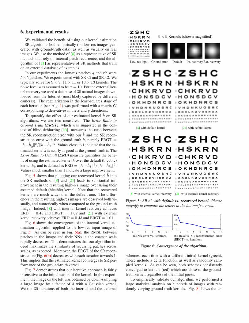
Fig. 5 shows that plugging our recovered kernel k into

the SR methods of [8] and [21] leads to substantial im-

provement in the resulting high-res image over using their

assumed default (bicubic) kernel. Note that the recovered

kernels are much wider than the default one. The differ-

ences in the resulting high-res images are observed both vi-

sually, and numerically when compared to the ground-truth

image. Indeed, [8] with internal kernel recovery achieves

ERD = 0.45 and ERGT = 1.02 and [21] with external

kernel recovery achieves ERD = 0.43 and ERGT = 1.01.

Fig. 6 shows the convergence of the internal kernel es-

timation algorithm applied to the low-res input image of

Fig. 5. As can be seen in Fig. 6(a), the RMSE between

patches in the image and their NNs in the coarser scale

rapidly decreases. This demonstrates that our algorithm in-

deed maximizes the similarity of recurring patches across

scales, as expected. Moreover, the ERGT of the SR recon-

struction (Fig. 6(b)) decreases with each iteration towards 1.

This implies that the estimated kernel converges to SR per-

formance of the ground-truth kernel.

Fig. 7 demonstrates that our iterative approach is fairly

insensitive to the initialization of the kernel. In this experi-

ment, the image on the left was obtained by down-sampling

a large image by a factor of 3 with a Gaussian kernel.

We ran 30 iterations of both the internal and the external

Low-res input

9× 9 Kernels (shown magnified):

Ground-truth Default Int. recovery Ext. recovery

[8] with default kernel [21] with default kernel

[8] with internal kernel recovery [21] with external kernel recovery

Figure 5: SR×2 with default vs. recovered kernel. Please

magnify to compare the letters at the bottom few rows.

2 4 6 8 10 12 1410

12

14

16

18

(a) NN error vs. iterations

2 4 6 8 10 12 14

1

1.5

2

2.5

(b) Relative SR reconstruction error(ERGT) vs. iterations

Figure 6: Convergence of the algorithm.

schemes, each time with a different initial kernel (green).

These include a delta function, as well as randomly sam-

pled kernels. As can be seen, both schemes consistently

converged to kernels (red) which are close to the ground-

truth kernel, regardless of the initial guess.

To empirically validate our algorithm, we performed a

large statistical analysis on hundreds of images with ran-

domly varying ground-truth kernels. Fig. 8 shows the er-

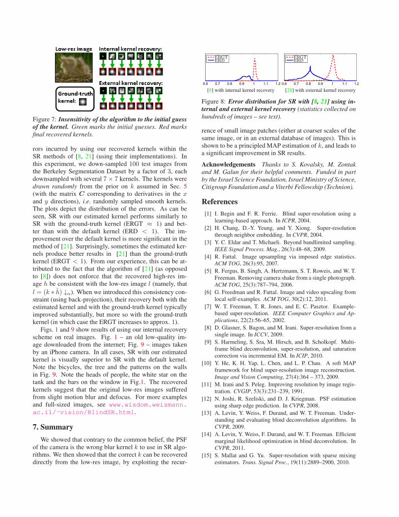
Figure 7: Insensitivity of the algorithm to the initial guess

of the kernel. Green marks the initial guesses. Red marks

final recovered kernels.

rors incurred by using our recovered kernels within the

SR methods of [8, 21] (using their implementations). In

this experiment, we down-sampled 100 test images from

the Berkeley Segmentation Dataset by a factor of 3, each

downsampled with several 7 × 7 kernels. The kernels were

drawn randomly from the prior on k assumed in Sec. 5

(with the matrix C corresponding to derivatives in the xand y directions), i.e. randomly sampled smooth kernels.

The plots depict the distribution of the errors. As can be

seen, SR with our estimated kernel performs similarly to

SR with the ground-truth kernel (ERGT ≈ 1) and bet-

ter than with the default kernel (ERD < 1). The im-

provement over the default kernel is more significant in the

method of [21]. Surprisingly, sometimes the estimated ker-

nels produce better results in [21] than the ground-truth

kernel (ERGT < 1). From our experience, this can be at-

tributed to the fact that the algorithm of [21] (as opposed

to [8]) does not enforce that the recovered high-res im-

age h be consistent with the low-res image l (namely, that

l = (k ∗ h) ↓α). When we introduced this consistency con-

straint (using back-projection), their recovery both with the

estimated kernel and with the ground-truth kernel typically

improved substantially, but more so with the ground-truth

kernel (in which case the ERGT increases to approx. 1).

Figs. 1 and 9 show results of using our internal recovery

scheme on real images. Fig. 1 – an old low-quality im-

age downloaded from the internet; Fig. 9 – images taken

by an iPhone camera. In all cases, SR with our estimated

kernel is visually superior to SR with the default kernel.

Note the bicycles, the tree and the patterns on the walls

in Fig. 9. Note the heads of people, the white star on the

tank and the bars on the window in Fig.1. The recovered

kernels suggest that the original low-res images suffered

from slight motion blur and defocus. For more examples

and full-sized images, see www.wisdom.weizmann.

ac.il/˜vision/BlindSR.html.

7. Summary

We showed that contrary to the common belief, the PSF

of the camera is the wrong blur kernel k to use in SR algo-

rithms. We then showed that the correct k can be recovered

directly from the low-res image, by exploiting the recur-

0.6 0.7 0.8 0.9 1 1.1 1.2

ERGTERD

[8] with internal kernel recovery

0.6 0.7 0.8 0.9 1 1.1 1.2

ERGTERD

[21] with external kernel recovery

Figure 8: Error distribution for SR with [8, 21] using in-

ternal and external kernel recovery (statistics collected on

hundreds of images – see text).

rence of small image patches (either at coarser scales of the

same image, or in an external database of images). This is

shown to be a principled MAP estimation of k, and leads to

a significant improvement in SR results.

Acknowledgements Thanks to S. Kovalsky, M. Zontak

and M. Galun for their helpful comments. Funded in part

by the Israel Science Foundation, Israel Ministry of Science,

Citigroup Foundation and a Viterbi Fellowship (Technion).

References

[1] I. Begin and F. R. Ferrie. Blind super-resolution using a

learning-based approach. In ICPR, 2004.

[2] H. Chang, D.-Y. Yeung, and Y. Xiong. Super-resolution

through neighbor embedding. In CVPR, 2004.

[3] Y. C. Eldar and T. Michaeli. Beyond bandlimited sampling.

IEEE Signal Process. Mag., 26(3):48–68, 2009.

[4] R. Fattal. Image upsampling via imposed edge statistics.

ACM TOG, 26(3):95, 2007.

[5] R. Fergus, B. Singh, A. Hertzmann, S. T. Roweis, and W. T.

Freeman. Removing camera shake from a single photograph.

ACM TOG, 25(3):787–794, 2006.

[6] G. Freedman and R. Fattal. Image and video upscaling from

local self-examples. ACM TOG, 30(2):12, 2011.

[7] W. T. Freeman, T. R. Jones, and E. C. Pasztor. Example-

based super-resolution. IEEE Computer Graphics and Ap-

plications, 22(2):56–65, 2002.

[8] D. Glasner, S. Bagon, and M. Irani. Super-resolution from a

single image. In ICCV, 2009.

[9] S. Harmeling, S. Sra, M. Hirsch, and B. Scholkopf. Multi-

frame blind deconvolution, super-resolution, and saturation

correction via incremental EM. In ICIP, 2010.

[10] Y. He, K. H. Yap, L. Chen, and L. P. Chau. A soft MAP

framework for blind super-resolution image reconstruction.

Image and Vision Computing, 27(4):364 – 373, 2009.

[11] M. Irani and S. Peleg. Improving resolution by image regis-

tration. CVGIP, 53(3):231–239, 1991.

[12] N. Joshi, R. Szeliski, and D. J. Kriegman. PSF estimation

using sharp edge prediction. In CVPR, 2008.

[13] A. Levin, Y. Weiss, F. Durand, and W. T. Freeman. Under-

standing and evaluating blind deconvolution algorithms. In

CVPR, 2009.

[14] A. Levin, Y. Weiss, F. Durand, and W. T. Freeman. Efficient

marginal likelihood optimization in blind deconvolution. In

CVPR, 2011.

[15] S. Mallat and G. Yu. Super-resolution with sparse mixing

estimators. Trans. Signal Proc., 19(11):2889–2900, 2010.

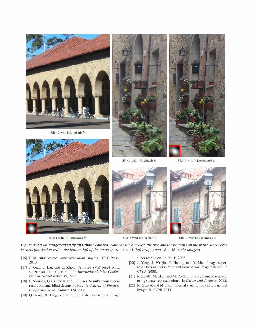
SR×2 with [8], default k

SR×2 with [8], estimated k

SR×3 with [8], default k SR×3 with [8], estimated k

SR×3 with [8], default k SR×3 with [8], estimated k

Figure 9: SR on images taken by an iPhone camera. Note the the bicycles, the tree and the patterns on the walls. Recovered

kernels (marked in red at the bottom-left of the images) are 11× 11 (left image) and 13× 13 (right images).

[16] P. Milanfar, editor. Super-resolution imaging. CRC Press,

2010.

[17] J. Qiao, J. Liu, and C. Zhao. A novel SVM-based blind

super-resolution algorithm. In International Joint Confer-

ence on Neural Networks, 2006.

[18] F. Sroubek, G. Cristobal, and J. Flusser. Simultaneous super-

resolution and blind deconvolution. In Journal of Physics:

Conference Series, volume 124, 2008.

[19] Q. Wang, X. Tang, and H. Shum. Patch based blind image

super resolution. In ICCV, 2005.

[20] J. Yang, J. Wright, T. Huang, and Y. Ma. Image super-

resolution as sparse representation of raw image patches. In

CVPR, 2008.

[21] R. Zeyde, M. Elad, and M. Protter. On single image scale-up

using sparse-representations. In Curves and Surfaces, 2012.

[22] M. Zontak and M. Irani. Internal statistics of a single natural

image. In CVPR, 2011.