Nonlinearity and Randomness in Complex Systems 1

Computing Waves in the Face of Uncertainty

E. Bruce PitmanDepartment of Mathematics

University at Buffalopitman@buffalo.edu

2

Part of a large project investigating geophysical mass flows Interdisciplinary research project funded by NSF (ITR and EAR)

UB departments/people involved: Mechanical engineering: A Patra, A Bauer, T Kesavadas, C

Bloebaum, A. Paliwal, K. Dalbey, N. Subramaniam, P. Nair, V. Kalivarappu, A. Vaze, A. Chanda

Mathematics: E.B. Pitman, C Nichita, L. Le Geology: M Sheridan, M Bursik, B.Yu, B. Rupp, A. Stinton, A. Webb,

B. Burkett Geography (National Center for Geographic Information and Analysis): C

Renschler, L. Namikawa, A. Sorokine, G. Sinha Center for Computational.Research M Jones, M. L. Green Iowa State University E Winer

3

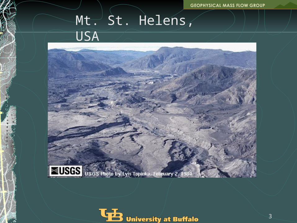
Mt. St. Helens, USA

4

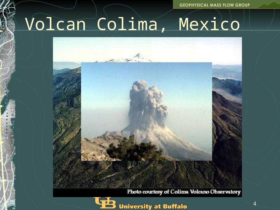
Volcan Colima, Mexico

5

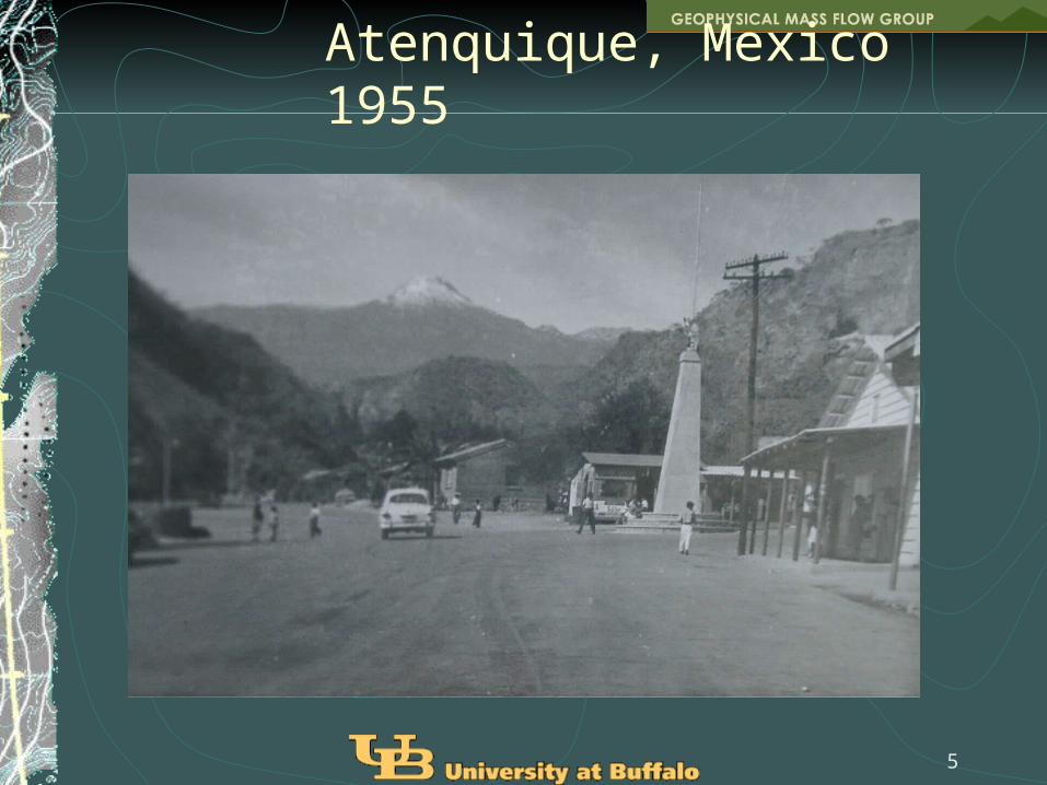
Atenquique, Mexico 1955

6

Atenquique, Mexico 1955

7

San Bernardino Mountain: Waterman Canyon

8

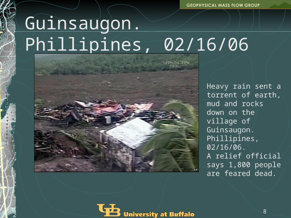
Guinsaugon. Phillipines, 02/16/06

Heavy rain sent a torrent of earth, mud and rocks down on the village of Guinsaugon. Phillipines, 02/16/06.A relief official says 1,800 people are feared dead.

9

Ruapehu, New Zealand

10

Pico de Orizaba, Mexico

Ballistic particle Simulations of pyroclastic flows and hazard map at Pico de Orizaba -- hazard maps by Sheridan et. al.

11

“Hazard map” based on flow simulations and input uncertainty characterizations

Regions for which probability of flow > 1m for initial volumes ranging from 5000 m3 to 108 m3 -- flow volume distribution from historical data

12

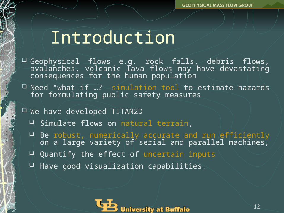
Introduction Geophysical flows e.g. rock falls, debris flows, avalanches, volcanic lava

flows may have devastating consequences for the human population Need “what if …?” simulation tool to estimate hazards for formulating public

safety measures

We have developed TITAN2D Simulate flows on natural terrain, Be robust, numerically accurate and run efficiently on a large variety of

serial and parallel machines, Quantify the effect of uncertain inputs Have good visualization capabilities.

13

Goals of this talk

Basic mathematical modeling Will not address extensions such as erosion, two

phase flows, that are important in the fieldUncertainty Quantification

Hyperbolic PDE system – poses special difficulties for uncertainty computations

Ultimate aim is Hazard Maps

Nonlinearity and Randomness in Complex Systems 14

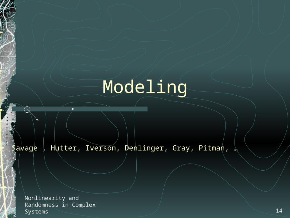
Modeling

Savage , Hutter, Iverson, Denlinger, Gray, Pitman, …

15

ModelingMany models – complex physics is still not perfectly represented !

Savage-Hutter ModelIverson-Denlinger mixture theory ModelPitman-Le Two-phase model

Debris Flows are hazardous mixture of soil, rocks, clasts with interstitial fluid present

16

Micromechanics and Macromechanics

Characteristic length scales (from mm to Km)

e.g. for Mount St. Helens (mudflow –1985) Runout distance 31,000 m Descent height 2,150 m Flow length(L) 100-2,000 Flow thickness(H) 1-10 m Mean diameter of sediment material 0.001-10 m

(data from Iverson 1995, Iverson & Denlinger 2001)

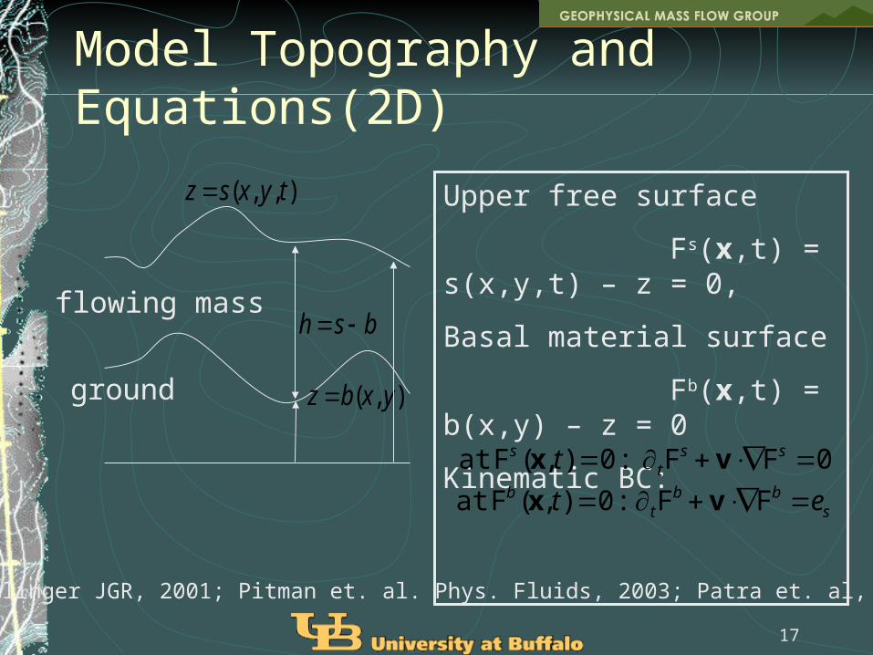
17

Model Topography and Equations(2D)

ground

flowing mass

),( yxbz

),,( tyxsz

bsh

Upper free surface

Fs(x,t) = s(x,y,t) – z = 0,

Basal material surface

Fb(x,t) = b(x,y) – z = 0

Kinematic BC:

sbb

tb

sst

s

et

t

FF:0),(Fat

0FF:0),(Fat

vx

vx

Iverson and Denlinger JGR, 2001; Pitman et. al. Phys. Fluids, 2003; Patra et. al, JVGR, 2005

18

Model System-Basic EquationsSolid Phase Only

gTuuu

u

000 ρρρ

0

t

The conservation laws for a continuum incompressible medium are:

stress-strain rate relationship derived from Coulomb theory

[Aside: this system of equations is ill-posed (Schaeffer 1987)]

Boundary conditions for stress:

bbb

r

rbbbbbbb

sss

t

t

nTnu

unTnnnTxF

nTxF

tan:0),(at

0:0),(at

: basal friction angle

19

Model System-Scaling

Scaling variables are chosen to reflect the shallownessof the geophysical mass

L – characteristic length in the downstream and cross-stream directions (Ox,Oy)

H – characteristic length in normal direction to the flow (Oz)Drop (most) terms of O()

**

**

****

ρ,

,),(

1/,,,,,

TT gHtL

gt

vvgLvv

LHHhhHzLyLxzyx

yxyx

20

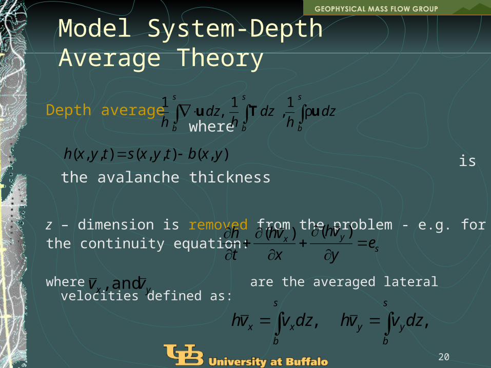
Model System-Depth Average Theory

Depth average where

is the avalanche thickness

z – dimension is removed from the problem - e.g. forthe continuity equation:

where are the averaged lateral velocities defined as:

s

b

s

b

s

b

dzh

dzh

dzh

uTu ρ1

,1

,1

),(),,(),,( yxbtyxstyxh

syx e

y

vh

x

vh

t

h

)()(

yx vv and,

s

b

yy

s

b

xx dzvvhdzvvh ,,

21

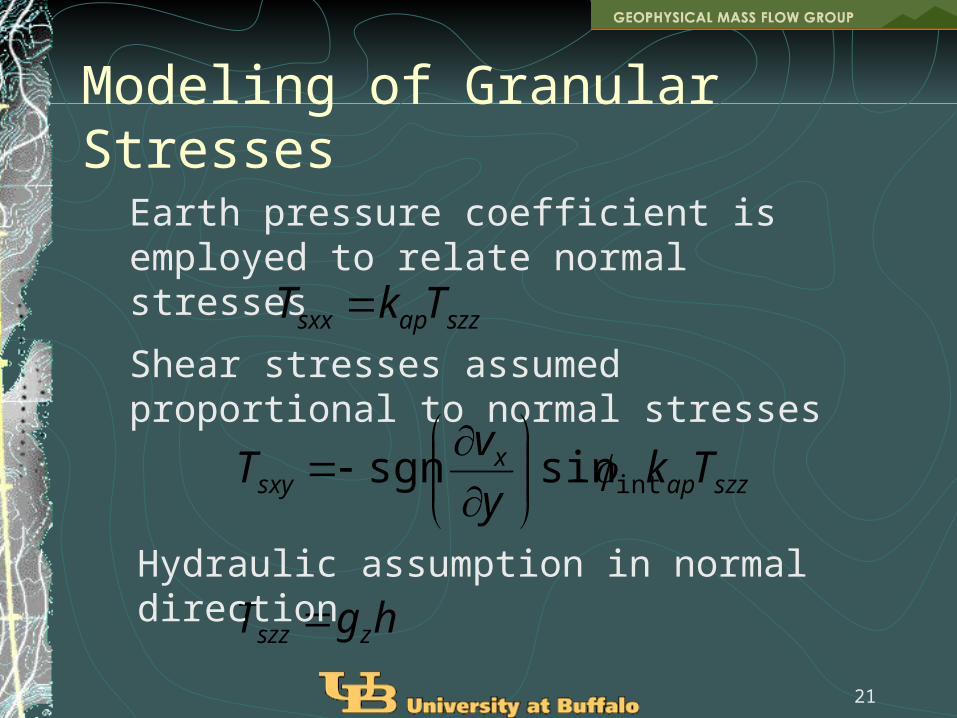
Modeling of Granular Stresses

szzapsxx TkT

Earth pressure coefficient is employed to relate normal stresses

Shear stresses assumed proportional to normal stresses

szzapx

sxy Tky

vT intsinsgn

hgT zszz Hydraulic assumption in normal direction

22

Depth averaging and scaling: Hyperbolic System of balance laws

continuity

x momentum

1. Gravitational driving force

2. Resisting force due to Coulomb friction at the base3. Intergranular Coulomb force due to velocity gradients normal to the

direction of flow

Model System – 2D

int2

22

22

sinsgntan1

)5.(

y

hghk

y

vhvg

vv

vevhg

y

vhv

x

hgkhv

t

hv

ey

hv

x

hv

t

h

zap

xbedx

xz

yx

xsxx

xyzapxx

syx

1 32

Nonlinearity and Randomness in Complex Systems 23

Uncertainty

Dalbey, Patra

24

Modeling and Uncertainty “Why prediction of grain behavior is difficult in geophysical granular

systems””

“…there is no universal constitutive description of this phenomenon as there is for hydraulics”

the variability of granular agglomerations is so large that fundamental physics is not capable of accurately describing the system and its variations

P. Haff (Powders and Grains ’97)

25

Uncertainty in Outputs of Simulations of Geophysical Mass Flows

Model UncertaintyModel Formulation: Assumptions and SimplificationsModel Evaluation: Numerical Approximation, Solution strategies – error estimation

Data Uncertainty propagation of input data uncertainty

26

Modeling Uncertainty• Sources of Input Data Uncertainty

Initial conditions – flow volume and position Bed and internal friction parameters Terrain errors Erosion and two phase model parameters

27

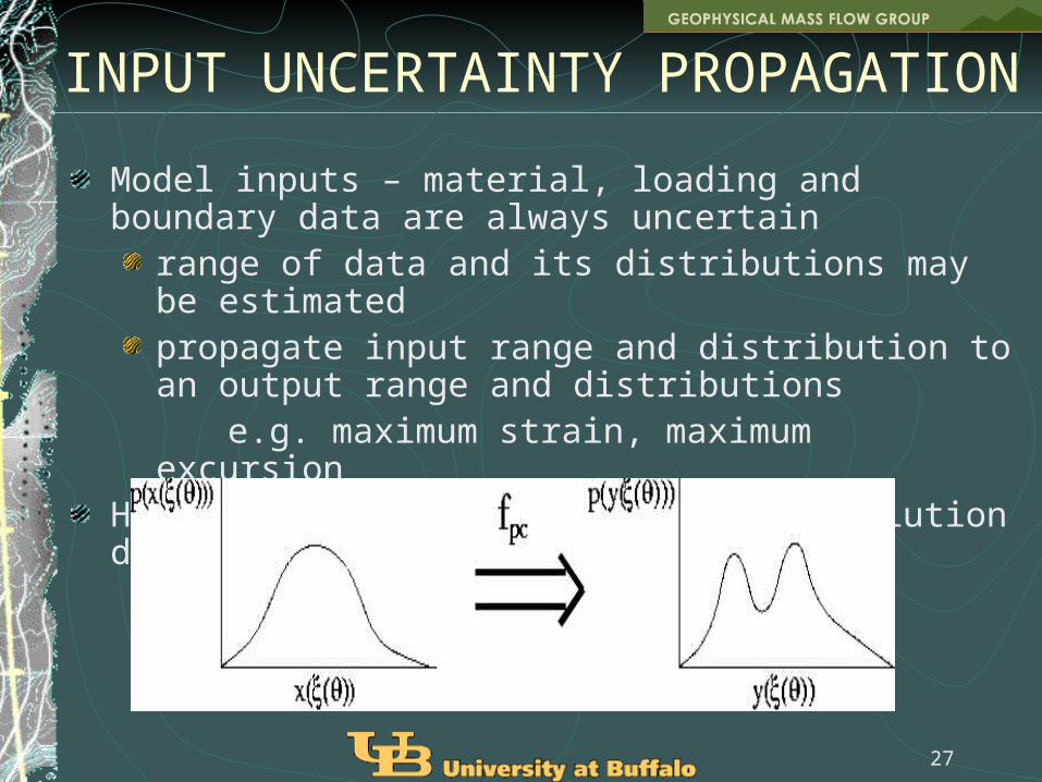
INPUT UNCERTAINTY PROPAGATION

Model inputs – material, loading and boundary data are always uncertain

range of data and its distributions may be estimatedpropagate input range and distribution to an output range and distributions

e.g. maximum strain, maximum excursionHow does uncertain input produce a solution distribution?

28

Effect of different initial volumes

Left – block and Ash flow on Colima, V =1.5 x 105 m3

Right – same flow -- V = 8 x105 m3

29

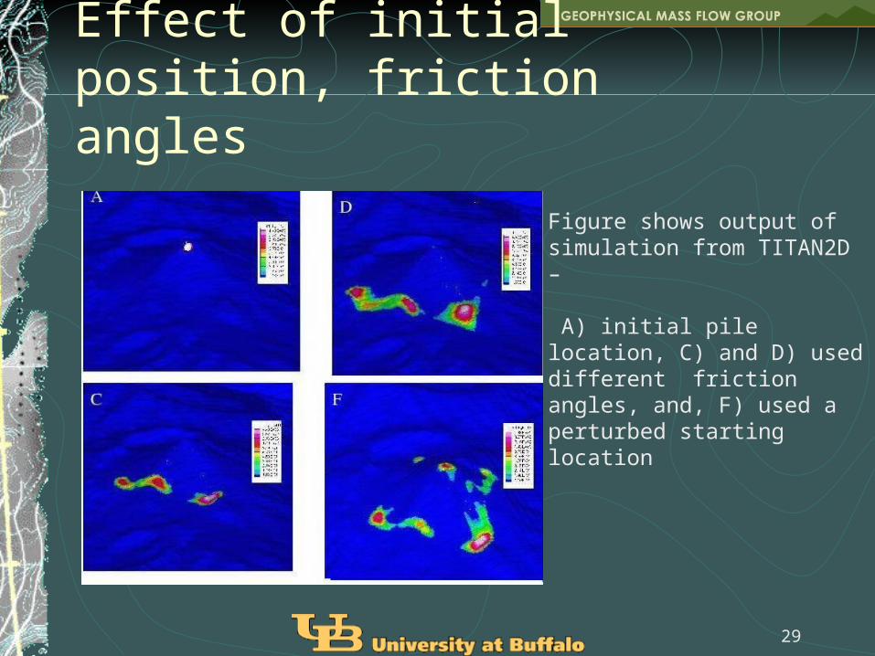
Effect of initial position, friction angles

Figure shows output of simulation from TITAN2D –

A) initial pile location, C) and D) used different friction angles, and, F) used a perturbed starting location

30

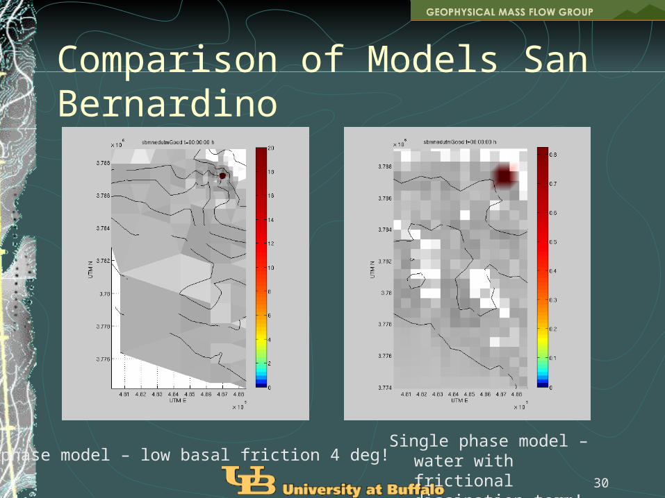
Comparison of Models San Bernardino

Single phase model – low basal friction 4 deg!Single phase model – water with

frictional dissipation term!

31

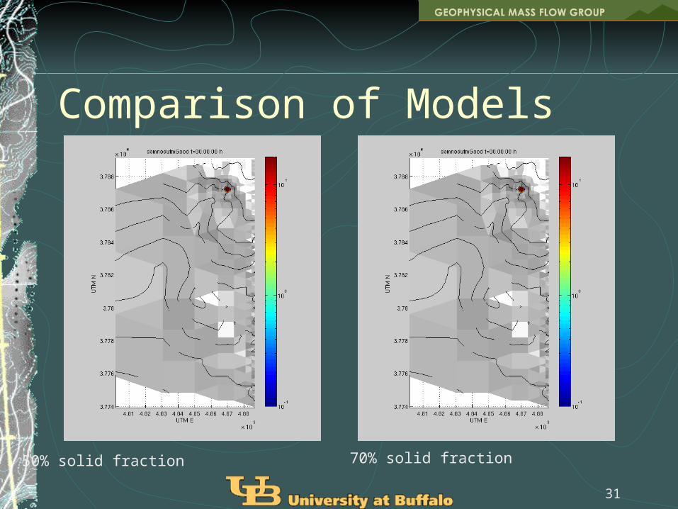
Comparison of Models

50% solid fraction 70% solid fraction

32

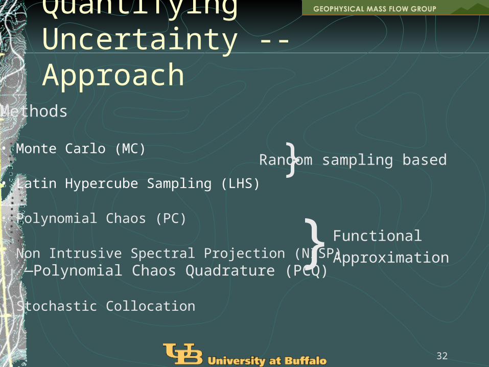
Quantifying Uncertainty -- ApproachMethods

• Monte Carlo (MC)

• Latin Hypercube Sampling (LHS)

• Polynomial Chaos (PC)

• Non Intrusive Spectral Projection (NISP)―Polynomial Chaos Quadrature (PCQ)

• Stochastic Collocation

}Random sampling based

} Functional Approximation

33

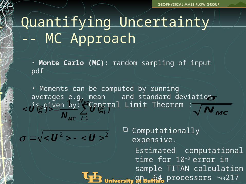
Quantifying Uncertainty -- MC Approach

• Monte Carlo (MC): random sampling of input pdf

• Moments can be computed by running averages e.g. mean and standard deviation is given by:

MCN

ii

MC

UN

U1

)(1

)(

22 UU

Central Limit Theorem :MCN

Computationally expensive. Estimated computational time for 10-3

error in sample TITAN calculation on 64 processors ~ 217 days

34

Latin Hypercube Sampling -- MMC

1. For each random direction (random variable or input), divide that direction into Nbin bins of equal probability;

2. Select one random value in each bin;

3. Divide each bin into 2 bins of equal probability; the random value chosen above lies in one of these sub-bins;

4. Select a random value in each sub-bin without one;

5. Repeat steps 3 and 4 until desired level of accuracy is obtained.

McKay 1979, Stein 1987, …

35

Functional ApproximationsIn these approaches we attempt to compute an approximation of the output pdf based on functional approximations of the input pdf

Prototypical method of this is the Karhunen Loeve expansion

37

Quantifying Uncertainty -- Approach

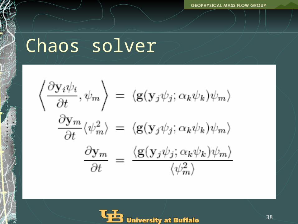
• Polynomial Chaos (PC): approximate pdf as the truncated sum of infinite number of orthogonal polynomials i

• Multiply by m and integrate to use orthogonality

Wiener ’34, Xiu and Karniadakis’02

))();(( tygt

y

)(

)()()(

jj

ii tyty

38

Chaos solver

39

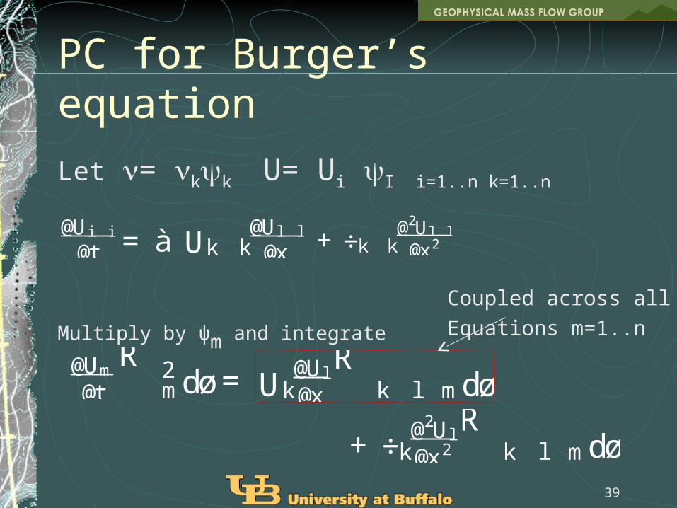
PC for Burger’s equationLet = kk U= Ui I i=1..n k=1..n

Multiply by ψm and integrate

@t@Ui i = à Uk k @x

@Ul l + ÷k k @x2@2Ul l

@t@Um

R 2

mdø= Uk@x@Ul

R k l mdø

+ ÷k@x2@2Ul

R k l mdø

Coupled across allEquations m=1..n

40

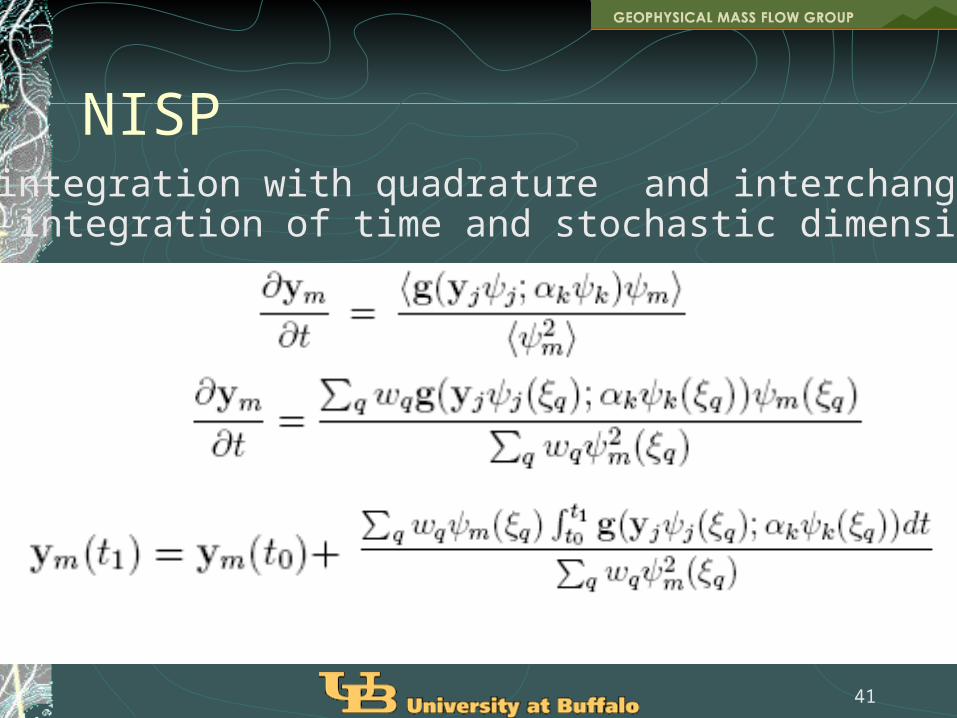
Polynomial Chaos QuadratureInstead of Galerkin projection, integrate by quadrature weightsAnalogy with Non-Intrusive Spectral Projection Stochastic Collocation

Leads to a method that has the simplicity of MC sampling and cost of PC Can directly compute all moment integralsEfficiency degrades for large number of random variables

41

NISPReplace integration with quadrature and interchangeorder of integration of time and stochastic dimension

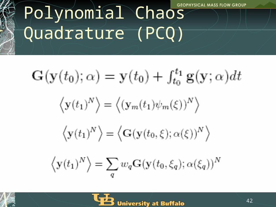
42

Polynomial Chaos Quadrature (PCQ)

44

Quantifying Uncertainty -- ApproachPCQ: a simple deterministic sampling method with sample points

chosen based on an understanding of PC and quadrature rules

makes PC computationally feasible for non-linear non-polynomial forms easy to implement and parallelize; statistics obtained directlycan use random variables from multiple distributions simultaneously

difficult to find sample points for very high orders“curse of dimensionality” -- samples required grows exponentially as a function of number of RV

45

Quantification of UncertaintyTest Problem

Application to flow at Volcan Colima

Starting location, and, Initial volume

are assumed to be random variables distributed according to assumption, or available data

46

Test ProblemBurgers equation

Figure shows statistics of time required to reachsteady state for randomlypositioned shock in initial condition; PCQ converges much fasterthan Monte Carlo

48

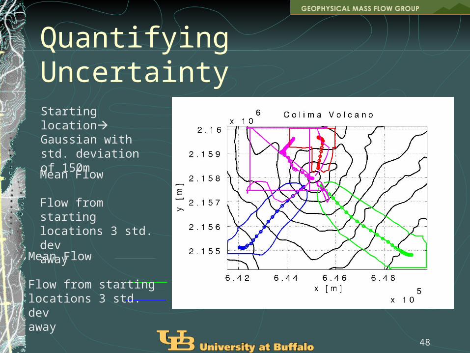
Quantifying UncertaintyStarting locationGaussian with std. deviation of 150m

Mean Flow

Flow from startinglocations 3 std. devaway

Mean Flow

Flow from startinglocations 3 std. devaway

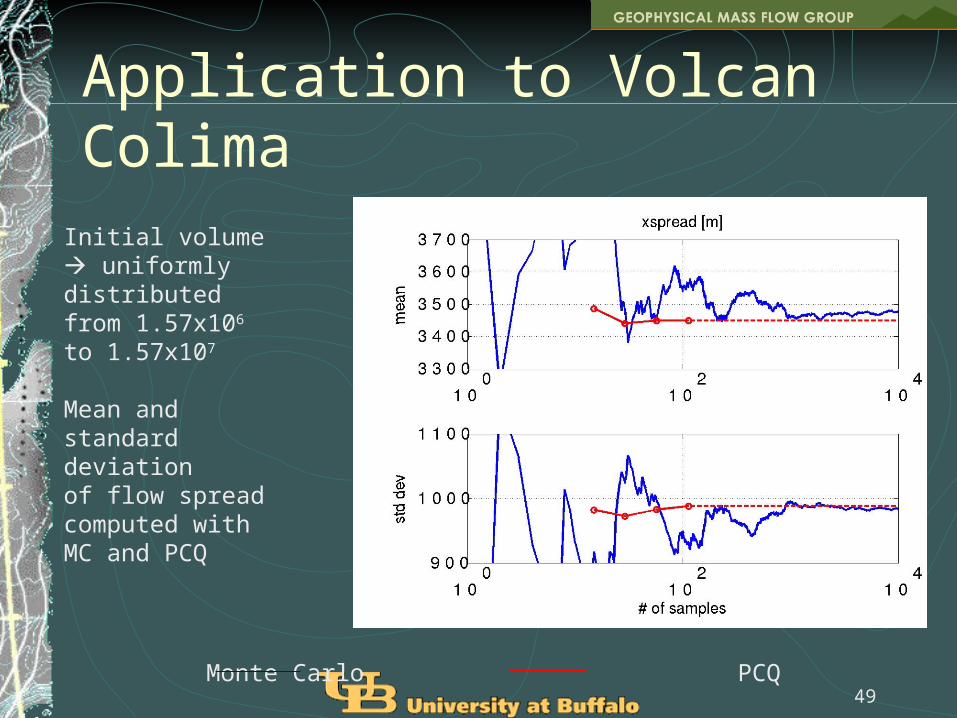
49

Application to Volcan ColimaInitial volume uniformlydistributed from 1.57x106

to 1.57x107

Mean and standard deviationof flow spread computed withMC and PCQ

Monte Carlo PCQ

50

Mean Flow for Volcan Colima for initial volume uncertainty

51

Mean+3std. dev for Volcan Colima -- initial volume uncertainty

52

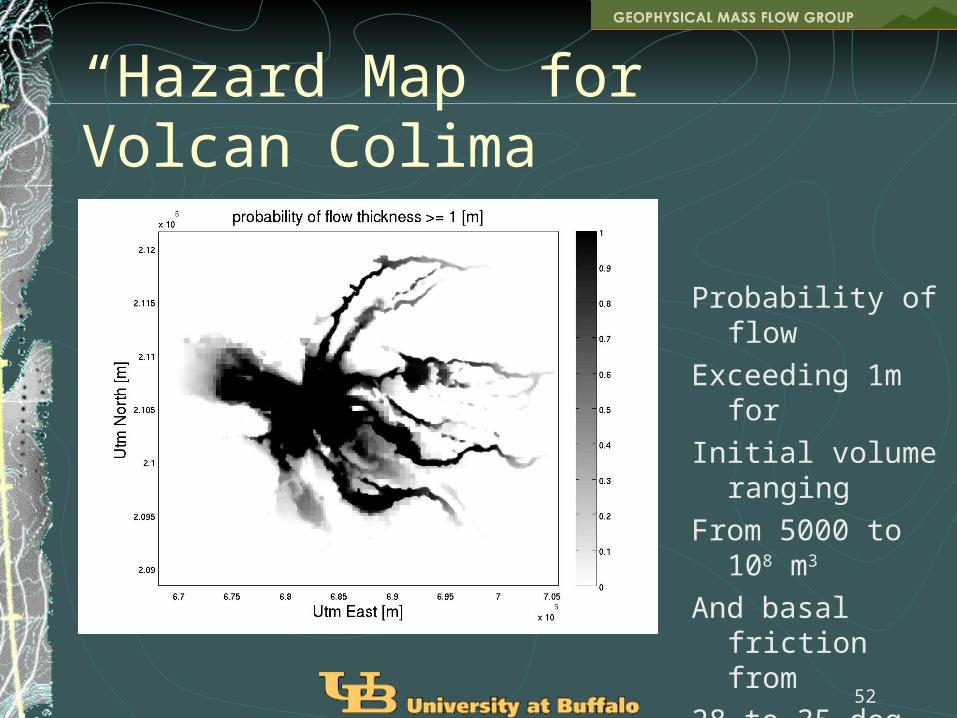
“Hazard Map” for Volcan Colima

Probability of flowExceeding 1m for Initial volume rangingFrom 5000 to 108 m3

And basal friction from28 to 35 deg

54

ConclusionsPCQ is an attractive methodology for

determining the solution distribution as a consequence of uncertainty

Find full pdfCurse of dimensionality still strikesMC, LH, NISP, Point Estimate methods, PCQ –

which to use depends on the problem at hand

55

Conclusions How to handle uncertainty in terrain? In the models? More work to integrate PCQ into output functionals that

prove valuable

All developed software is available free and open source from www.gmfg.buffalo.edu

Software can be accessed on the Computational Grid (DOE Open Science Grid) at http://grid.ccr.buffalo.edu