nonlinear2dtransformations: deconstructingpathscass/graphics/manual/pdf/ch8.pdf · chapter 8....

CHAPTER 8

Nonlinear 2D transformations:

deconstructing paths

Sometimes wewant to draw a figure after a nonlinear transformation has been applied to it. In imagemanipula

tion programs, this is often calledmorphing . For example, here is a morphed 10×10 grid produced by a programin which the basic drawing commands drew a square grid and these were followed by some transforming code

before stroking.

In order to apply transformations to paths, we just have to understand (a) transformations and (b) paths!

8.1. Two dimensional transformations

A 2D transformation is a function f(x, y) of two variables which returns a pair of numbers u(x, y) and v(x, y),the coordinates of the transform of the point (x, y). We have already seen affine transformations where

f(x, y) = (ax + by + c, dx + ey + f)

for suitable constants a, b, etc. But now we want to allow more complicated ones. I should say right at thebeginning that these can be very complicated. An affine transformation is not so difficult to visualize because we

know what the transformation does everywhere if we know what it does to just a single square. But an arbitrarytransformation may have very different effects in different parts of the plane, and this is the source of much

difficulty in comprehending it. Indeed, the nature of 2D transformations has been in notsodistant times the

subject of interesting mathematical research. (I am referring to the stability of properties of such transformationsunder perturbation, part of the socalled ‘catastrophe theory’.)

I’ll spend some time looking at one which is not too complicated:

f(x, y) = (x2 − y2, 2xy) .

This is not quite a random choice—it is derived from the function of complex numbers that takes z to z2, since

(x + iy)2 = (x2 − y2) + i (2xy) .

Chapter 8. Nonlinear 2D transformations: deconstructing paths 2

The best way to understand what it does is to write (x, y) in polar coordinates as (r cos θ, r sin θ), since in theseterms f takes (x, y) to

(r2 cos2 θ − r2 sin θ, 2r2 cos θ sin θ) = (r2 cos 2θ, r2 sin 2θ) .

In other words, it squares r and doubles θ. We can see how this works in the following figures. On the left is thesector of the unit circle between 0 and π/2, on the right its image with respect to f :

That seems simple enough. And yet, the image that began this chapter is the transformation with respect to this

same f of the square with lower left corner at (1/2, 0), upper right at (3/2, 1), sides aligned with the axes. Soeven this simple transformation has some interesting effects. We’ll see others when we look at what it does to

character strings.

A transformation is completely described by the formula for its separate components, i.e. the functions u and vin the expression

f(x, y) = (u(x, y), v(x, y)) .

This is all we’ll need to know about f in order to apply it. But in order to understand in any deep sense how atransformation in 2D behaves, we also must consider its Jacobian derivative . This is a matrixvalued function ofx and y whose entries are the partial derivatives of f :

Jacf (x, y) =

∂u∂x

∂v∂x

∂u∂y

∂v∂y

.

For the example we have already looked at this is

[

2x 2y−2y 2x

]

.

The importance of the Jacobian matrix is that it allows us to approximate the map f by an affine map in any smallneighbourhood of a point. The exact statement is:

• If∆x and∆y are small then we have an approximate equality

f(x + ∆x, y + ∆y) ≈ f(x, y) + [ ∆x ∆y ] Jacf (x, y)

Another way to say it:

• If (x, y) lies near (x0, y0) then we have an approximate equality

f(x, y) ≈ f(x0, y0) + [ (x − x0) (y − y0) ] Jacf (x, y) .

What this says, roughly, is that locally in small regions the transformation looks as though it were affine.

This phenomenon can be seen geometrically. If we look at the figure that started this chapter, but zoom in, wesee:


In other words, if we zoom in to a part of the plane, the transformation looks straighter and straighter as the

scale shrinks. I’ll not say much more about why this Jacobian approximation is valid, but only remark thatit is essentially the definition of partial derivatives. It is the generalization to 2D of the linear approximation

f(x + ∆x) ≈ f(x) + f ′(x)∆x encountered in the ordinary calculus of one variable.

In our example, we have an exact equation

f(x + ∆x, y + ∆y) = ((x + ∆x)2 − (y + ∆y)2, 2(x + ∆x)(y + ∆y))

= ((x2 + 2x∆x + ∆x2) − (y2 + 2y∆y + ∆y2), 2(xy + x∆y + y∆x + ∆x∆y)

which becomes

((x2 + 2x∆x) − (y2 + 2y∆y), 2(xy + x∆y + y∆x) ≈ (x2 − y2, 2xy) + [2x∆x − 2y∆y, 2x∆y + y∆x]

= f(x, y) + [ ∆x ∆y ]

[

2x 2y−2y 2x

]

if we ignore the terms of order two—i.e. ∆x2, ∆y2, ∆x∆y. But this linear approximation is the Jacobian

approximation. As it always is.

I’ll not use the Jacobian derivative in PostScript procedures, although it could conceivably improve quality at the

cost of complication. But it is important to realize that the reason our transformation procedures will work sowell is precisely because in very small regions the function f looks affine.

In routines to be described later, a 2D transformation f will be given as a procedure with two arguments x andy, and it will return a pair u v. In our example it would be

% on stack: x y

/fcn { 2 dict begin

/y exch def

/x exch def

x dup mul y dup mul sub % x^2-y^2

2 x mul y mul % 2xy

end } def

It would in principle be possible to get a smoother output if I added a second version that takes advantage of the

Jacobian approximation. In this version the function f would return the Jacobian matrix on the stack as well, inthe form of an array of 4 variables. In practice this doesn’t seem to be important.


8.2. Conformal transforms

As we have seen, the Jacobian matrix of the transform (x, y) 7→ (x2 − y2, 2xy) is

[

2x 2y−2y 2x

]

.

This matrix has the form[

a b−b a

]

,

and such matrices, which I’ll call similarity matrices for reasons that will become apparent in a moment, have

interesting properties. One example of such a matrix is the rotation matrix

[

cos θ sin θ− sin θ cos θ

]

,

and another is the scalar matrix[

rr

]

,

So also is the product of these two[

r cos θ r sin θ−r sin θ r cos θ

]

.

In fact, if S is any similarity matrix[

a b−b a

]

,

We can writea√

a2 + b2= cos θ

b√a2 + b2

= sin θ

and then

[

a b−b a

]

=

[

r cos θ r sin θ−r sin θ r cos θ

]

where r =√

a2 + b2, so that every similarity matrix is the product of a rotation and a scaling.

• A matrix is a similarity matrix if and only if (1) it has positive determinant and (2) the linear transformationassociated to it is a similarity transformation—that is to say, it preserves the shape of figures.

In particular, a similarity transformation takes squares to (possibly larger or smaller) squares, which explains

what we have seen in the pictures of the map (x, y) 7→ (x2 − y2, 2xy).

In general, a transform from 2D to 2D is called conformal if its Jacobian matrix is a similarity matrix at all buta few isolated points. Such a map looks like a similarity transformation in small regions, and hence preserves

the angles between paths, even though it may distort large shapes wildly. Thus the map (x, y) 7→ (x2 − y2, 2xy)is conformal, except at the origin (where it doubles angles). As I mentioned before, this map was derived from

the map z 7→ z2 of complex numbers. There is a huge class of similar complexvalued functions of a complex

variable which are conformal.


8.3. Transforming paths

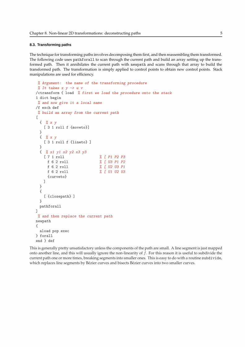
The technique for transforming paths involves decomposing themfirst, and then reassembling them transformed.

The following code uses pathforall to scan through the current path and build an array setting up the transformed path. Then it annihilates the current path with newpath and scans through that array to build the

transformed path. The transformation is simply applied to control points to obtain new control points. Stack

manipulations are used for efficiency.

% Argument: the name of the transforming procedure

% It takes x y -> u v

/ctransform { load % first we load the procedure onto the stack

1 dict begin

% and now give it a local name

/f exch def

% build an array from the current path

[

{ % x y

[ 3 1 roll f {moveto}]

}

{ % x y

[ 3 1 roll f {lineto} ]

}

{ % x1 y1 x2 y2 x3 y3

[ 7 1 roll % [ P1 P2 P3

f 6 2 roll % [ U3 P1 P2

f 6 2 roll % [ U2 U3 P1

f 6 2 roll % [ U1 U2 U3

{curveto}

]

}

{

[ {closepath} ]

}

pathforall

]

% and then replace the current path

newpath

{

aload pop exec

} forall

end } def

This is generally pretty unsatisfactory unless the components of the path are small. A line segment is just mapped

onto another line, and this will usually ignore the nonlinearity of f . For this reason it is useful to subdivide thecurrent path one ormore times, breaking segments into smaller ones. This is easy to dowith a routine subdivide,which replaces line segments by Bezier curves and bisects Bezier curves into two smaller curves.


8.4. Maps

The classical examples of 2D transformations, although with an implicit 3D twist, occur in the design of maps of

the Earth. The basic problem is that there is no faithful way to render the surface of a sphere on a flat surface.There is no one single kind of map that does for all purposes, and various kinds must be designed to conform to

various criteria.

Coordinates on the sphere are East longitude x and latitude y. Assuming the Earth’s surface to be a sphere ofradius R, the coordinate map takes

(x, y) 7−→ (R cosx cos y, R sin x cos y, R sin y) .

The image of a small rectangle dx× dy is an approximate rectangle in space of dimensions R cos y dx×R dy. Ofcourse the coordinates are singular near the poles, since the poles have indeterminate longitude.

I’ll assume from now on for convenience that R = 1. (This is just a matter of choosing units of lengths correctly.)

The simplest map just transforms longitude and latitude into x and y:

There’s not much to be said for it. It preserves distance measured along meridians, but distorts wildly distances

along parallels.


The next simplestmap is called the cylindrical projection , because it projects a point on the Earth’s surface straightout to a vertical cylinder wrapped around the Earth, touching at the Equator. Explicitly,

(x, y) 7−→ (x, sin y) .

It was proven by Archimedes in his classic ‘On sphere and cylinder’ that this map preserves areas, although it

certainly distorts distances near the poles. The modern proof that area is preserved calculates that the regioncos y dx × dy maps to that of dimensions dx × cos y dy.

A more interesting one is the Mercator projection

(x, y) 7→(

x, ln tan(π/4 + y/2))

.


Here, distances and areas near the poles are grossly exaggerated, but angles are conserved, so that plotting a

route by compass is relatively simple. Indeed this is exactly the purpose for which this projection was designed.The first map of this sort was constructed by the 16th century geographer Gerardus Mercator himself, but it was

likely the Englishman Thomas Harriot who understood its mathematical basis thoroughly—well, as thoroughly

as could be done without calculus.

Why is the Mercator map conformal? Recall that the image of a small coordinate rectangle dx by dy is veryapproximately a rectangle on the sphere of dimensions cos y dx × dy. Its image under Mercator’s map has sizedx by

tan′(π/4 + y/2) dy =dy

cos y.

But these two rectangles are similar to each other, with a scale factor of 1/ cosy. In other words, the functiontan(π/4 + y/2) has been chosen precisely because its derivative is 1/ cosy.

All of the maps exhibited here were obtained from the original map data by applying ctransform.

8.5. Stereographic projection

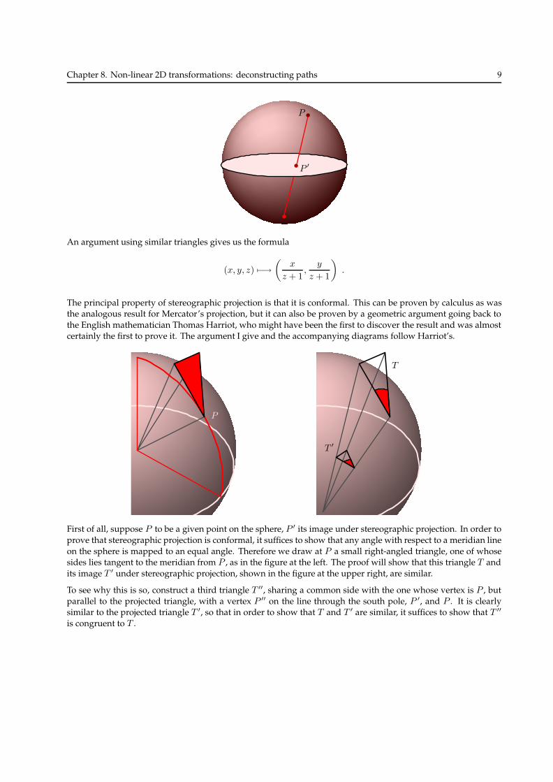
Another map projection, stereographic projection , deserves a section all to itself, since it plays an important

role in much mathematics. In this projection, a point P on a sphere is mapped to the intersection P ′ of the linesegment from P to the south pole with the equatorial plane.


P

P ′

An argument using similar triangles gives us the formula

(x, y, z) 7−→(

x

z + 1,

y

z + 1

)

.

The principal property of stereographic projection is that it is conformal. This can be proven by calculus as wasthe analogous result for Mercator’s projection, but it can also be proven by a geometric argument going back to

the English mathematician Thomas Harriot, who might have been the first to discover the result and was almostcertainly the first to prove it. The argument I give and the accompanying diagrams follow Harriot’s.

P

T

T ′

First of all, suppose P to be a given point on the sphere, P ′ its image under stereographic projection. In order to

prove that stereographic projection is conformal, it suffices to show that any angle with respect to a meridian line

on the sphere is mapped to an equal angle. Therefore we draw at P a small rightangled triangle, one of whosesides lies tangent to the meridian from P , as in the figure at the left. The proof will show that this triangle T andits image T ′ under stereographic projection, shown in the figure at the upper right, are similar.

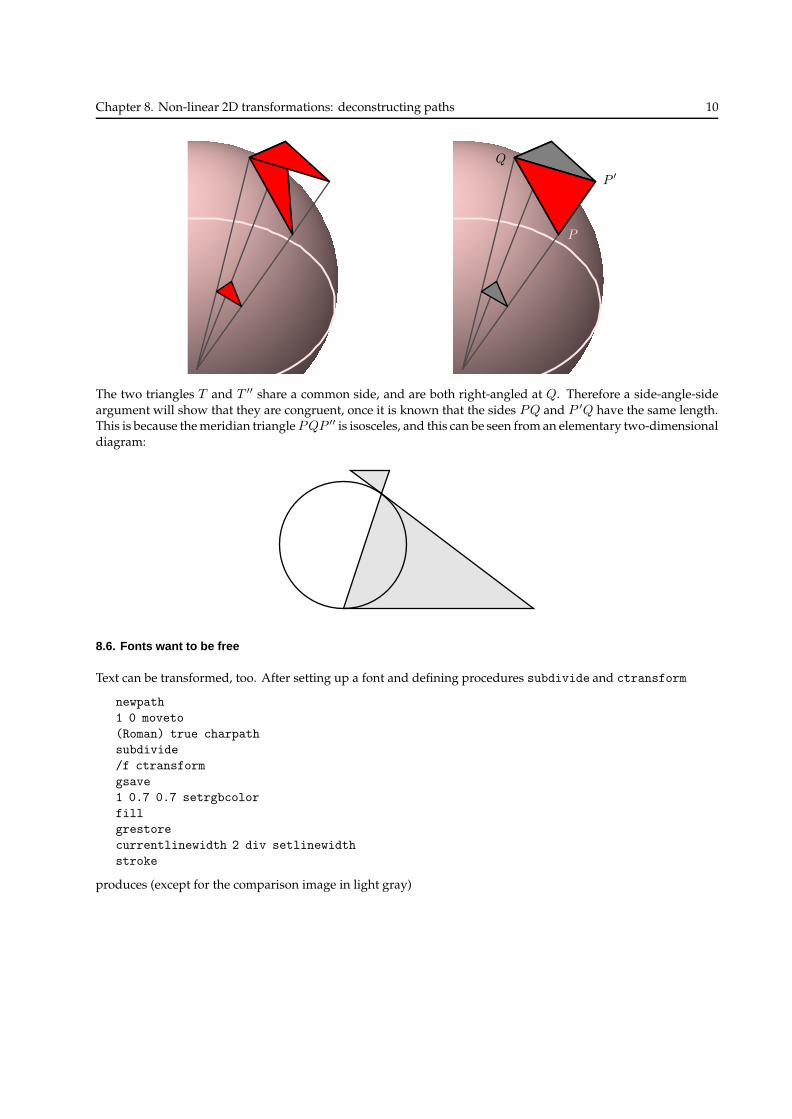
To see why this is so, construct a third triangle T ′′, sharing a common side with the one whose vertex is P , butparallel to the projected triangle, with a vertex P ′′ on the line through the south pole, P ′, and P . It is clearlysimilar to the projected triangle T ′, so that in order to show that T and T ′ are similar, it suffices to show that T ′′

is congruent to T .


P

P ′

Q

The two triangles T and T ′′ share a common side, and are both rightangled at Q. Therefore a sideanglesideargument will show that they are congruent, once it is known that the sides PQ and P ′Q have the same length.This is because themeridian trianglePQP ′′ is isosceles, and this can be seen from an elementary twodimensional

diagram:

8.6. Fonts want to be free

Text can be transformed, too. After setting up a font and defining procedures subdivide and ctransform

newpath

1 0 moveto

(Roman) true charpath

subdivide

/f ctransform

gsave

1 0.7 0.7 setrgbcolor

fill

grestore

currentlinewidth 2 div setlinewidth

stroke

produces (except for the comparison image in light gray)


RomanSubdivision is important here because font paths possess a lot of straight segments which are much better off

transformed as curves.

8.7. Code

The procedures subdivide and ctransform are to be found in the package transform.inc. The map data can

be found in the PostScript files coasts.1.inc etc, which I have made from the MWDB files mentioned below. The

index indicates level of detail—index 1 is the greatest detail, index 5 the least.

References

1. J. L. Berggren and A. Jones, Ptolemy’s Geography , Princeton University Press, 1997. Mathematical mapmaking began with the Greeks. The illustrations here, many taken from medieval manuscripts, are beautiful.

The invention of printed books in theWest meant not only a wider audience for science but also, ironically, a loss

in the quality of graphics and in particular the loss of brilliant colour.

2. TimothyG. Freeman, Portraits of the Earth—A mathematician looks at maps , AmericanMathematical Society,

2002. An appendix includes an account of howwhat seems to be the same map data that I have used can be usedto draw maps using Maple.

3. David Hilbert and Stephan CohnVossen, Geometry and the Imagination , Chelsea, 1952. Many maps areconformal—preserve angles—and one of the basic theorems in the subject is that stereographic projection is

a conformal map. Nowadays this can be proven quickly by calculus, but an elegant geometric proof can be

found in §36 of this book. Early Greek astronomers knew that stereographic projection maps circles to circles,applying a theorem of Apollonius on conic sections to deduce it. This fact is closely related to conformality,

but conformality itself was apparently first stated and proved by the English mathematician Thomas Harriot,

who was among other things Sir Walter Raleigh’s navigation expert, in about 1590. This was still in the goldenage of mapmaking stimulated by the discovery and exploration of America, as well as the great Portugese

voyages around Africa to the Far East. Harriot’s proof was unpublished, but it can be reconstructed from a ratherhandsome sketch in his manuscripts. A reproduction can be found in the article by J. A. Lohne, ‘Thomas Harriot

als Mathematiker’, Centaurus 11 (1965/66), who also discusses Harriot’s treatment of the Mercator projection.The first published proof was by Edmund Halley, who is often (and incorrectly) given credit for it. His paperis ‘An Easie Demonstration of the Analogy of the Logarithmic Tangents . . . ’ in the Philosophical Transactions19 (1695–1697), pp. 202–214 (miraculously available through the electronic library service JSTOR). Althoughhe acknowledges that he learned the statement from De Moivre he claims the proof as his own, but there issuspicion that both came one way one way or another from the remarkable Harriot (as did probably much other

mathematics of the 17th century).

4. John McCleary, Geometry from a differentiable viewpoint , Cambridge University Press, 1994. There is an

interesting account of map projections in Chapter 8 which, like much of this book, would serve nicely as a sourceof graphics projects.

5. Tristan Needham, Visual Complex Analysis , Oxford University Press, 1997. This explains the relationshipbetween complex numbers and conformal maps with lots of illustrations.

6. John P. Snyder, Flattening the Earth: Two Thousand Years of Map Projections , University of Chicago Press,

1993. This is a very readable history of mapmaking, including descriptions of dozens of different ones.


7. For the maps I have used the data from the ‘World Database II’, which is now included in the file world.zip

accessible by clicking on the icon at

http://archive.msmonline.com/1999/12/vis2.htm

These map data, which are now in the public domain, were compiled by Fred Pospeschil and Antonio Riveria

from data originally created by the Central intelligence Agency. The particular files I have used incorporatefurther modifications by by Paul Anderson of Global Associates, Ltd. The Bodleian Library of Oxford University

maintains a convenient web page with links to sources of other map data available without cost.

nonlinear2dtransformations: deconstructingpathscass/graphics/manual/pdf/ch8.pdf · chapter 8....

Documents