nonlinear transformation and application of treasury bond …
TRANSCRIPT

IJRRAS 42 (1) ● Jan 2020 www.arpapress.com/Volumes/Vol42Issue1/IJRRAS_42_1_03.pdf
24
NONLINEAR TRANSFORMATION AND APPLICATION OF TREASURY
BOND PRICING BASED ON VASICEK MODEL
Huang Yitao and Zhang Jingjing* [email protected]
College of Science, University of Shanghai for Science and Technology, Shanghai 200093, PR China
ABSTRACT
Vasicek model is one of the most classic models in the theory on term structure of interest rate. However, Vasicek
model has a weakness, i.e. The drift function on linearity of instantaneous short rate does not correspond to actual
features of interest rate. To overcome the weakness, based on Vasicek model, the paper linear conducts
transformation, and verifies non-linear Vasicek model through the method of ordinary least squares(OLS). Then,
Monte Carlo simulation is adopted to analyze the pricing of treasury bond, and compare pricing differences before
and after transformation. According to results of analysis, transformed Vasicek model is more suitable for treasury
bond pricing.
Keywords: Treasury Bond Pricing, Vasicek Model, OLS Test, Monte Carlo Simulation.
1. INTRODUCTION
After over three decades of development, the bond market has achieved rapid development in China. Investments
and financing functions have been greatly enhanced as well. Until the end of 2018, total transactions of Chinese
bond market were worth more than 8 trillion RMB. Bond issuers mainly include commercial banks, policy
banks,Ministry of Finance, IFC and ordinary enterprises,etc. Hypothecating type repurchase, open repurchase,
forward transaction, cash transaction are the main types of bond transactions. With the constant development of
bond market, more importance will be attached to treasury bond pricing and interest rate risk management. What
needs to be pointed out is that one type of bond has always been important and unique in the market, which is
treasury bond.
Domestic scholars do not pay much attention to treasury bond pricing or compile a lot of documents on model
innocation. Wen Zhongqiao (2004) adopted three common factors to analyze treasury bond pricing in China.
According to the research, model estimated by one-week bond redemption interest rate indicates the most apparent
effect of pricing. Moreover, errors of bond pricing increase with the extension of bond duration. Zhou Rongxi and
Wang Xiaoguang (2011) utilized MCMC simulation method to estimate the parameters of Vasicek model and CIR
model, and conducted relevant studies on bond pricing. According to the results, treasury bond market prices are
generally higher than prices estimated by the two models. In addition, as bond duration extends, pricing errors also
increase constantly.
Foreign scholars pay more attention to research on treasury bond pricing, and many breakthroughs on model
innovation were achieved. Robert and Yildiray(2003) utilized HJM model to analyze the pricing of TIPS and
derivative products. For John,Turalay and Martin(2009), Markov borough system was utilized to convert CIR
model and analyzed the new model, indicating the new model showed more apparent effects of pricing than original
CIR model. Tak(2010 formulated a Markov borough system, converted by Vasicek model. According to his
analysis, transformed model was more superior than original Vasicek mode. Jens,Lopez and
Rudebusch(2012)built the arbitrage-free model with chance fluctuation rate, and analyzed TIPS with deflation
protection.
However, in the above-mentioned documents, linear interest rate model was frequently utilized. However, up to this
day, more and more evidence has shown that interest rates have non-linear traits. For this reason, non-linearization
will be a measure of practical significance. Due to simple structures and convenient estimation of Vasicek model, it
is frequently adopted in assets pricing. This paper will conduct non-linear transformation of Vasicek model, and
apply it to analyze treasury bond pricing.
2. PRICING PRINCIPLE OF VASICEK MODEL
In this section, conventional perspective is ignored. In other words, the concept of risk neutral probability measure is
not used to discuss the pricing principle of Vasicek model. Instead, a new and easy-to-understand method is
adopted, i.e. The pricing principle of Vasicek model is analyzed through formulating risk-free assets portfolios.
There are mainly three steps involved. Firstly, partial differential equations of zero coupon bond prices should apply

IJRRAS 42 (1) ● Jan 2020 Yitao & Jingjing ● Treasury Bond Pricing Based on Vasicek Model
25
to single-factor dynamic model, i.e. term structure equation. Secondly, utilize unique traits of Vasicek model in the
partial differential equation, in order to obtain the analytic expression of zero coupon bond price. Lastly, the
discount rate should be concluded based on the capital and price of zero coupon bonds, so as to estimate the price of
treasury bond according to the cash flow of the discount rate . Next, the process of detailed deduction is shown as
follows. Assume the differential equation of instantaneous rate is:
( , ) ( , ) (2.1)t t t tdr r t dt r t dW = +
( , ), ( , )t tr t r t are drift function and spread function, and a known form of another certain function. tW
is
Brownian movement. Assume the price of zero coupon bond is ( , , )tP r T t . T represents the term of maturity for
zero coupon bond. Then, the differential value of ( , , )tP r T t is
22
2
1( ) (2.2)
2
P P PdP dt dr dr
t r r
= + +
Note that Ito's Lemma is used in the above equation. Combine the the above two equation and obtain the following: 2
2
2
1( ( , ) ( , )) ( , ) (2.3)
2t t t t
P P P PdP r t r t dt r t dW
t r r r
= + + +
Note that Ito's Lemma is also used in the above process of combining equations. Then, two zero coupon bonds with
different maturity dates are adopted to forge a risk-free of asset portfolio, and we assume the combination is Z in the
following:
1 2( , , ) ( , , ) (2.4)t tZ P r T t kP r T t= +
T1 and T2 are two random dates of maturity. Next, a k of proper ratio or position is selected to ensure zero interest
rate risk for the combination, i.e.
1 2( , , ) ( , , )0 (2.5)t tP r T t P r T t
kr r
+ =
Ito's differential of Z is concluded:
221 1 1
2
1 2 2
222 2
2
( , , ) ( , , ) ( , , )1[ ( , ) ( , )]
2
( , , ) ( , , ) ( , , )( , ) [ ( , )
( , , ) ( , , )1( , )] ( , ) (2.6)
2
t t tt t
t t tt t t
t tt t t
P r T t P r T t P r T tdZ r t r t dt
t r r
P r T t P r T t P r T tr t dW k r t
r t r
P r T t P r T tr t dt k r t dW
r r
= + +
+ + +
+ +
Equation (2.5) is incorporated into the above one:
221 1 1
2
222 2 2
2
( , , ) ( , , ) ( , , )1[ ( , ) ( , )]
2
( , , ) ( , , ) ( , , )1[ ( , ) ( , )] (2.7)
2
t t tt t
t t tt t
P r T t P r T t P r T tdZ r t r t dt
t r r
P r T t P r T t P r T tk r t r t dt
t r r
= + +
+ + +
( , )tr t is retained so that subsequent deduction is explicit and easy to understand. Considering Combination Z is
risk-free, its rate of return and risk-free return are consistent with each other, i.e.:
(2.8)t
dZr
Zdt=
Equation (2.7) is incorporated to the above:
IJRRAS 42 (1) ● Jan 2020 Yitao & Jingjing ● Treasury Bond Pricing Based on Vasicek Model
26
221 1 1
12
1
222 2 2
22
2
( , , ) ( , , ) ( , , )1( ( , ) ( , )) ( , , )
2( , , )
( , )
( , , ) ( , , ) ( , , )1( ( , ) ( , )) ( , , )
2 (2.9)( , , )
( , )
t t tt t t t
tt
t t tt t t t
tt
P r T t P r T t P r T tr t r t r P r T t
t r rP r T t
r tr
P r T t P r T t P r T tr t r t r P r T t
t r rP r T t
r tr
+ + −
+ + −
=
Because T1,T2 are random, we may denote them as:
22
2
( , , ) ( , , ) ( , , )1[ ( , ) ( , )] ( , , )
2( , ) (2.10)( , , )
( , )
t t tt t t t
tt
t
P r T t P r T t P r T tr t r t r P r T t
t r rc r tP r T t
r tr
+ + −
=
Next, equation (2.10) is adjusted to obtain partial differential equation to partial differential equation on zero coupon
bond: 2
2
2
( , , ) ( , , ) ( , , )1[ ( , ) ( , ) ( , )] ( , ) ( , , ) 0 (2.11)
2
t t tt t t t t t
P r T t P r T t P r T tr t c r t r t r t r P r T t
t r r
+ − + − =
The boundary condition is:
( , , ) 1 (2.12)tP r T T =
What is worth noting is: The boundary condition unitizes the debenture capital to simplify equation analysis and
calculation. In order to solve the above partial differential equation, we need to consider unique traits of Vasicek
model. According to viewpoints and conclusions of Vasicek(1978), we assume the price of zero coupon bond is: ( )
( , , ) ( ) (2.13)tB T t r
tP r T t A T t e− −
= −
A、B is the unknown function of (T-t). Beside, we also can learn:
( , ) ( ), ( , ) , ( , ) (2.14)t t t tr t r r t c r t c = − = =
(2.11) is simplified as:
22
2
1[ ( ) ] (2.15)
2
P P Pr c rP
r t r
− − + + =
(2.13) is incorporated to the above equation:
22
2
' '
exp( )
exp( ) (2.16)
exp( ) exp( )
PAB rB
r
PAB rB
r
PrAB rB A rB
t
= − −
= −
= − − − A' and B' are the differential coefficients of A and B respectively. (2.16)is included in (2.11) to obtain:
' 2 2 '1( ) [( ) ] 0 (2.17)
2r AB AB A c B B A A + − + − + − =
Due to the randomness of r, functions A and B are acquired based on the following two differential equations: '
2 2 '
1
(2.18)1[( ) ] 0
2
B B
c B B A A
+ =
− + − =
As the boundary condition (2.12) of partial differential equation is valid to any random r, we can also redefine the
boundary condition of differential equation(2.18):
(0) 1, (0) 0 (2.19)A B= =

IJRRAS 42 (1) ● Jan 2020 Yitao & Jingjing ● Treasury Bond Pricing Based on Vasicek Model
27
The following equations are obtained from (2.18)and(2.19).
( )
2 2 22 ( )
2 2 3
( ) (1 ) /
(2.20)( ) exp[ ( ) ( )( ) (1 ) ]
2 4
T t
T t
B T t e
c cA T t B T t e
− −
− −
− = −
− = − − − − − − + −
So far, we have completely obtained the expression of zero coupon bond price. In order to get the price of treasury
bond, we assume discount rate as vt, and conclude the following:
( )( , , )
(2.21)1ln ( , , )
tv T t
t
t t
P r T t e
v P r T tT t
− − =
= −−
Lastly, according to the theory on continuous compounding discounts, treasury bond price can be defined as:
( ) (2.22)tv t
t
D CF t e−
=
t is the time for repayment of principle or issuance of interest. CF is cash flow.
3. ESTABLISHMENT OF NON-LINEAR VASICEK MODEL
Observe the differential form of Vasicek model:
0 1( ) ( ( )) ( ) (3.1)dr t a a r t dt dW t= + +
0 1, ,a a are constants.W(t) is Brownian movement. It is not hard to find out a unique trait of equation (3.1): Drift
function of Vasicek model is linear function of instantaneous interest rate. However, more and more evidence has
proven that drift function of Vasicek model is non-linear function of instantaneous interest rate. Foreign scholars,
such as Ait-Sahalia(1997)and Stanton(1998), conducted non-linear test on the drift function of Vasicek model
through non-parametric ways, indicating that drift function and instantaneous interest rate are non-linear. Domestic
scholars, such as Lin Hai and Hong Yongsen(2007), built different models of dynamic interest rates and terms.
According to empirical analysis, models with non-linear drift functions can apparently reduce errors of fitting. In
addition, Hu Jinjin(2014) and Sun Hao(2015) found that models of non-linear dynamic interest rate term structures
can more accurately describe the dynamic changes of interest rate. As many predecessors’ research and studies have
achieved reliable results from non-linear tests, the main purpose of this paper is to correspond to the results of
predecessors rather than explore unknown fields. Therefore, scatter diagram, which is a simple and direct method, is
used in non-linear tests on drift function of Vasicek model. The theoretical foundation is Eulerian discretion of
Vasicek model.
1 0 1 1( ) ( ) ( ) (3.2)i i i ir t r t a a r t Z+ +− = + +
Zi+1 is random variable that comply with standard normal distribution. According to equation (3.2), we find out an
apparent trait: linear relation is shown by interest rate spread between previous term and next term,as well as interest
rate level of previous term. In fact, this trait is equivalent to the trait of equation (3.1), but the previous one is in
differential form. We may also regard it as a continuous form, which is more suitable for theoretical deduction and
verification. The latter one depicts the recurrence relation of interest rate sequence, which is more applicable to
empirical analysis, especially in the current era of superb calculation of computers. In this paper, the data of
overnight repo rates for treasury bonds in 2018, 2017 and 2016 are utilized. The results of non-linear test and drift
function are shown in the following figure:
IJRRAS 42 (1) ● Jan 2020 Yitao & Jingjing ● Treasury Bond Pricing Based on Vasicek Model
28
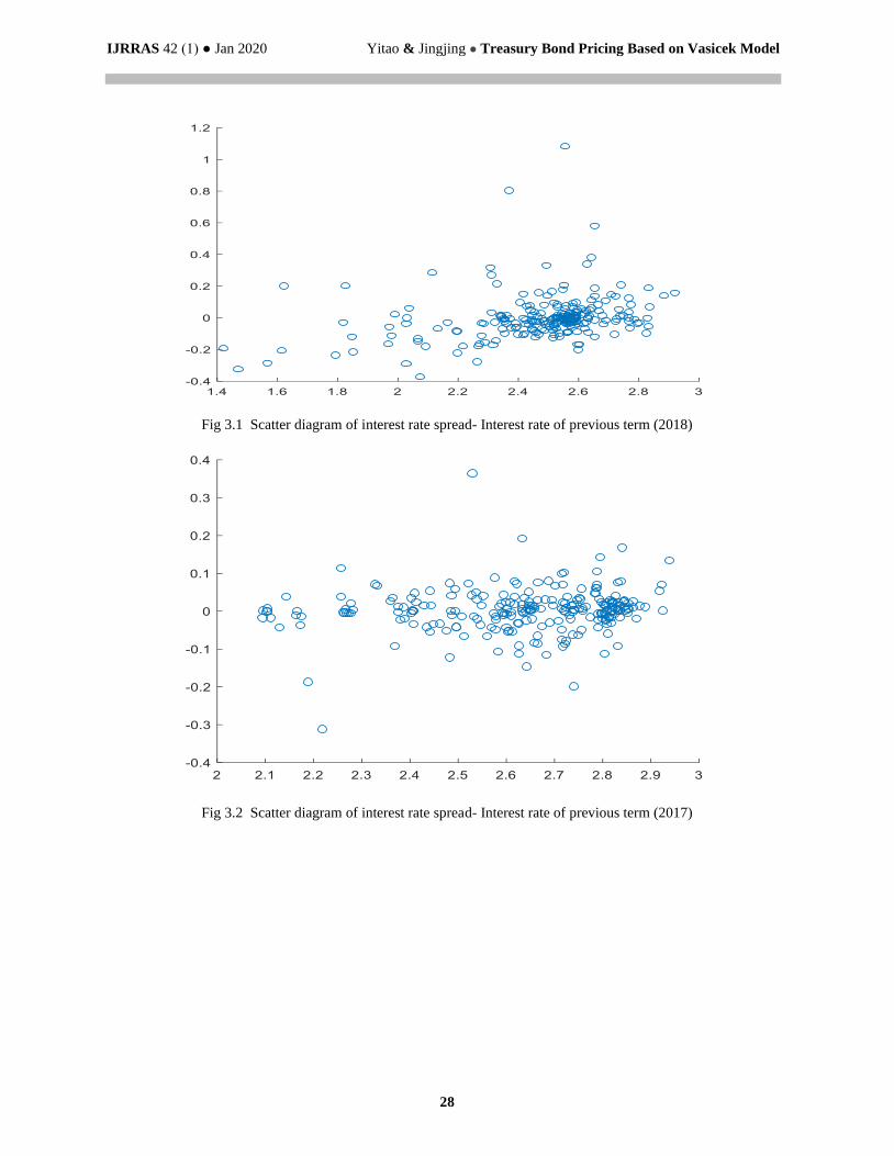
Fig 3.1 Scatter diagram of interest rate spread- Interest rate of previous term (2018)
Fig 3.2 Scatter diagram of interest rate spread- Interest rate of previous term (2017)
IJRRAS 42 (1) ● Jan 2020 Yitao & Jingjing ● Treasury Bond Pricing Based on Vasicek Model
29
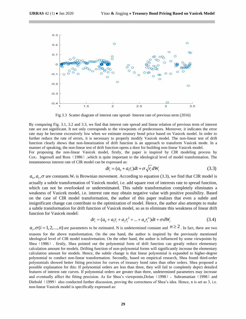
Fig 3.3 Scatter diagram of interest rate spread- Interest rate of previous term (2016)
By comparing Fig. 3.1, 3.2 and 3.3, we find that interest rate spread and linear relation of previous term of interest
rate are not significant. It not only corresponds to the viewpoints of predecessors. Moreover, it indicates the error
rate may be become excessively low when we estimate treasury bond price based on Vasicek model. In order to
further reduce the rate of errors, it is necessary to properly modify Vasicek model. The non-linear test of drift
function clearly shows that non-linearization of drift function is an approach to transform Vasicek mode. In a
manner of speaking, the non-linear test of drift function opens a door for building non-linear Vasicek model.
For proposing the non-linear Vasicek model, firstly, the paper is inspired by CIR modeling process by
Cox,Ingersoll and Ross(1986),which is quite important to the ideological level of model transformation. The
instantaneous interest rate of CIR model can be expressed as:
0 1( ) (3.3)t t t tdr a a r dt r dW= + +
0 1, ,a a are constants.Wt is Brownian movement. According to equation (3.3), we find that CIR model is
actually a subtle transformation of Vasicek model, i.e. add square root of interests rate to spread function,
which can not be overlooked or underestimated. This subtle transformation completely eliminates a
weakness of Vasicek model, i.e. interest rate may obtain negative value with positive possibility. Based
on the case of CIR model transformation, the author of this paper realizes that even a subtle and
insignificant change can contribute to the optimization of model. Hence, the author also attempts to make
a subtle transformation for drift function of Vasicek model, so as to eliminate this weakness of linear drift
function for Vasicek model: 2
0 1 2( ... ) (3.4)n
t t t n t tdr a a r a r a r dt dW= + + + + +
, ( 1,2,..., )ia i n = are parameters to be estimated. N is undetermined constant and 2n . In fact, there are two
reasons for the above transformation. On the one hand, the author is inspired by the previously mentioned
ideological level of CIR model transformation. On the other hand, the author is influenced by some viewpoints by
Shea(1986). firstly, Shea pointed out the polynomial form of drift function can greatly reduce elementary
calculation amount for models. Drifting function of non-polynomial forms will significantly increase the elementary
calculation amount for models. Hence, the subtle change is that linear polynomial is expanded to higher-degree
polynomial to conduct non-linear transformation. Secondly, based on empirical research, Shea found third-order
polynomials showed better fitting precision for curves of treasury bond rates than other orders. Shea proposed a
possible explanation for this: If polynomial orders are less than three, they will fail to completely depict detailed
features of interest rate curves. If polynomial orders are greater than three, undetermined parameters may increase
and eventually affect the fitting precision. As for Shea’s viewpoints,Dolan(1998),Subramanian(1998)and
Diebold(1999)also conducted further discussion, proving the correctness of Shea’s idea. Hence, n is set as 3, i.e.
non-linear Vasicek model is specifically expressed as:

IJRRAS 42 (1) ● Jan 2020 Yitao & Jingjing ● Treasury Bond Pricing Based on Vasicek Model
30
2 3
0 1 2 3( ) (3.5)t t t t tdr a a r a r a r dt dW= + + + +
0 1 2 3, , , ,a a a a are parameters to be estimated. After the non-linear Vasicek model is proposed, this section
discusses the final process of building non-linear Vasicek model,i.e. conduct model test. Comparison test method is
utilized. To be more specific, OLS test results of non-linear Vasicek model are compared with the results of OLS
test on original Vasicek model. If the former outweighs the latter, the model is valid. Otherwise, the model should be
rebuilt. In fact, the underlying principle of comparison test method strives for the better rather than the best. Even if
it is a minor improvement, we still have to recognize and accept it. For this OLS comparison test, the data on
overnight repo rates of treasury bonds in 2018,2017 and 2016 are adopted. Specific test results are shown in the
following table:
Table 3.1 OLS test comparison (2018)
OLS test based on Vasicek model
Estimated
value
Standard
deviation T statistic P value
Goodness
of Fit F statistic
a0 0.089 0.028 3.221 0.001
0.201 158.871 a1 -0.055 0.026 3.119 0.002
sigma 0.014 0.026 2.446 0.015
OLS test based on non-linear Vasicek model
Estimated
value
Standard
deviation T statistic P value
Goodness
of Fit F statistic
a0 -0.023 0.039 3.119 0.002
0.502 298.452
a1 0.074 0.023 3.501 0.001
a2 -0.018 0.023 3.804 0.000
a3 0.067 0.027 2.933 0.004
sigma 0.014 0.031 2.778 0.006
Table 3.2 OLS test comparison (2017)
OLS test based on Vasicek model
Estimated
value
Standard
deviation T statistic P value
Goodness
of Fit F statistic
a0 0.087 0.037 2.988 0.003
0.204 163.331 a1 -0.052 0.022 3.509 0.001
sigma 0.018 0.032 2.228 0.027
OLS test based on non-linear Vasicek model
Estimated
value
Standard
deviation T statistic P value
Goodness
of Fit F statistic
a0 -0.024 0.038 3.244 0.001
0.511 308.156
a1 0.078 0.024 3.343 0.001
a2 -0.022 0.021 3.877 0.000
a3 0.059 0.031 2.886 0.004
sigma 0.017 0.033 2.612 0.010

IJRRAS 42 (1) ● Jan 2020 Yitao & Jingjing ● Treasury Bond Pricing Based on Vasicek Model
31
Table 3.3 OLS test comparison (2016)
OLS test based on Vasicek model
Estimate
d value
Standard
deviation T statistic
P
value
Goodnes
s of Fit F statistic
a0 0.086 0.019 3.444 0.001
0.198 140.966 a1 -0.058 0.027 3.108 0.002
sigma 0.017 0.028 2.309 0.022
OLS test based on non-linear Vasicek model
Estimate
d value
Standard
deviation T statistic
P
value
Goodnes
s of Fit F statistic
a0 -0.025 0.031 3.298 0.001
0.499 290.012
a1 0.079 0.031 2.834 0.005
a2 -0.021 0.028 2.774 0.006
a3 0.057 0.033 2.772 0.006
sigma 0.019 0.029 2.835 0.005
Based on Table 3.1, 3.2 and 3.3, we find that goodness of fit and F statistic for non-linear Vasicek model are greater
than original Vasicek model. In other words, fitting effects and overall significance of non-linear Vasicek model
have been superior to original Vasicel mode. Hence, we contend that non-linear Vasicek model passes OLS test. To
put it in another way, this model is already built. Since non-linear Vasicek model has been established, we should
apply this new model in some empirical analysis. In this paper, we utilize this new model to discuss the pricing
strategy of treasury bond.
4. APPLICATION OF NON-LINEAR VASICEK MODEL
There is a difficult problem concerning the application of non-linear Vasicek model in analyzing treasury bond
price. Once we add high-order items in the drift function of original model, we can not obtain the explicit solution of
the partial differential equation on zero coupon bond prices, or interest bond prices. However, we may utilize Monte
Carlo simulation method to determine treasury bond pricing. First of all, we need to learn about the concept of
Monte Carlo simulation. Monte Carlo simulation, which is also known as random sampling test method, is an
important branch of numerical mathematics. The basic principle and ideology is: When the problem to be solved is
the probability of a certain event or expectation of a random variable, the above-mentioned issues can lead to sample
mean values of this random variable or actual frequency of event occurrence based on a certain “test” method. The
pricing principle of Monte Carlo simulation primarily shows three parts in this section :(1) Computer software is
used in Monte Carlo simulation to generate n paths of interest rates, denoted as( ), 1,2,...,iR t i n=
. (2) Discount
cash flow along every path of interest rate, so as to estimate prices of n treasury bonds: ( )
( ) , 1,2,..., (4.1)iR t t
i
t
P CF t e i n−
= =
CF(t) is the cash flow of treasury bonds at t. (3) Calculate prices of n treasury bonds to get the final estimated prices
of n treasury bonds, i.e.
1
(4.2)n
i
i
P P=
=
After discussing the pricing principle of Monte Carlo simulation, this section will conduct demonstration. Ten
representative treasury bonds are selected in pricing analysis, whose basic information in shown in the following
table:

IJRRAS 42 (1) ● Jan 2020 Yitao & Jingjing ● Treasury Bond Pricing Based on Vasicek Model
32
Table 4.1 Basic information of relevant treasury bonds
No. Bond Type Bond Code Nominal
Interest
Payment of
Annual Interest
Maturity
Data
1 21 Treasury(7) 010107 4.26% 2 2021/7/31
2 03 Treasury(3) 010303 3.40% 2 2023/4/17
3 05 Treasury(4) 010504 4.11% 2 2025/5/15
4 05 Treasury(12) 010512 3.65% 2 2020/11/15
5 06 Treasury(19) 010619 3.27% 2 2021/11/15
6 10 Treasury(12) 019012 3.25% 2 2020/5/13
7 12 Treasury(18) 019218 4.10% 2 2032/9/27
8 13 Treasury(3) 019303 3.42% 1 2020/1/24
9 13 Treasury(8) 019308 3.29% 1 2020/4/18
10 15 Treasury(8) 019508 4.09% 2 2035/4/27
According to Table 3.1, we can obtain the non-linear Vasicek estimation model that applied to overnight repo rates
of treasury bonds in 2018: 2 3( 0.023 0.074 0.018 0.067 ) 0.014 (4.3)t t t t tdr r r r dt dW= − + − + +
Eulerian discretion is conducted to obtain the recurrence relation of interest rate:
2 3
1 1( 0.023 0.074 0.018 0.067 ) 0.014 (4.4)t t t t t tr r r r r t tZ+ += + − + − + +
Fig. 4.1 Interest rate paths of Monte Carlo simulation
In order for computers to analyze Equation (4.4) through Monte Carlo simulation, four factors should be identified.
(1) Identify t in this paper, 1/ 360t = .(2) Identify first item. The first item can truly initiated based on
recurrence relation. A lot of documents use average interest rate as the index, in this paper, the first item is decided
as the average value of overnight repo rates in 2018, r0=0.031. (3) Decided the number of days for simulation. Table
4.1 shows the latest data of maturity for the ten treasury bonds is 2035/4/27, i.e. the longest residual maturity is no
IJRRAS 42 (1) ● Jan 2020 Yitao & Jingjing ● Treasury Bond Pricing Based on Vasicek Model
33
more than 17 years. Hence, in this paper, 6200 days are decided for the simulation, which will cover the interest rate
paths of the ten treasury bonds. (4) Decide the number of interest rate paths. The paper consulted a lot of documents,
concluding that 5000 paths are enough to depict the complexity and randomness of market interest. Fig. 4.1 shows
the Monte Carlo simulation result.
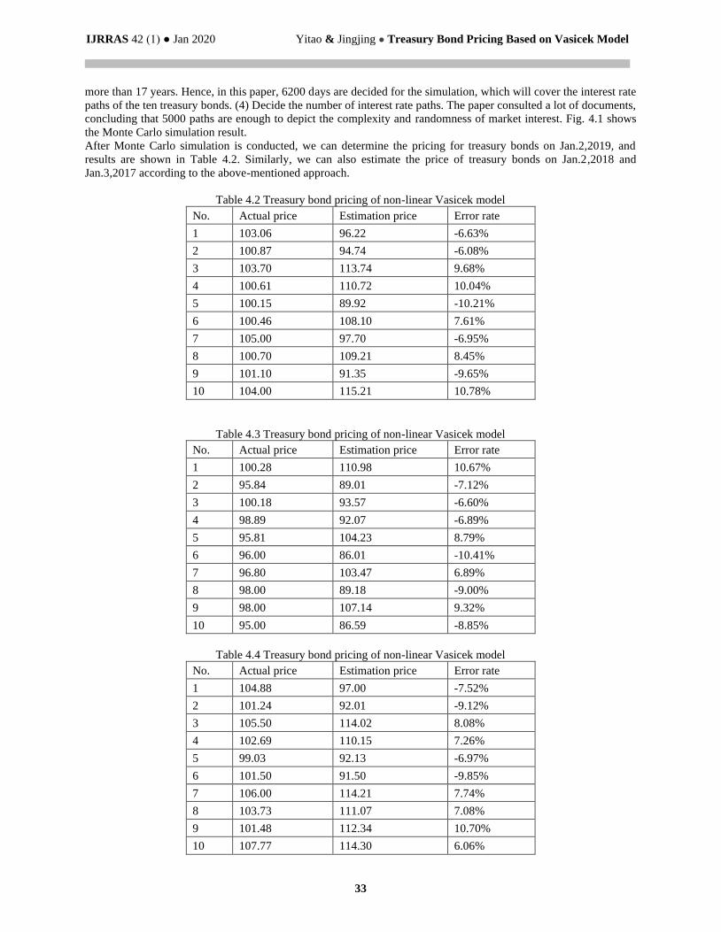
After Monte Carlo simulation is conducted, we can determine the pricing for treasury bonds on Jan.2,2019, and
results are shown in Table 4.2. Similarly, we can also estimate the price of treasury bonds on Jan.2,2018 and
Jan.3,2017 according to the above-mentioned approach.
Table 4.2 Treasury bond pricing of non-linear Vasicek model
No. Actual price Estimation price Error rate
1 103.06 96.22 -6.63%
2 100.87 94.74 -6.08%
3 103.70 113.74 9.68%
4 100.61 110.72 10.04%
5 100.15 89.92 -10.21%
6 100.46 108.10 7.61%
7 105.00 97.70 -6.95%
8 100.70 109.21 8.45%
9 101.10 91.35 -9.65%
10 104.00 115.21 10.78%
Table 4.3 Treasury bond pricing of non-linear Vasicek model
No. Actual price Estimation price Error rate
1 100.28 110.98 10.67%
2 95.84 89.01 -7.12%
3 100.18 93.57 -6.60%
4 98.89 92.07 -6.89%
5 95.81 104.23 8.79%
6 96.00 86.01 -10.41%
7 96.80 103.47 6.89%
8 98.00 89.18 -9.00%
9 98.00 107.14 9.32%
10 95.00 86.59 -8.85%
Table 4.4 Treasury bond pricing of non-linear Vasicek model
No. Actual price Estimation price Error rate
1 104.88 97.00 -7.52%
2 101.24 92.01 -9.12%
3 105.50 114.02 8.08%
4 102.69 110.15 7.26%
5 99.03 92.13 -6.97%
6 101.50 91.50 -9.85%
7 106.00 114.21 7.74%
8 103.73 111.07 7.08%
9 101.48 112.34 10.70%
10 107.77 114.30 6.06%

IJRRAS 42 (1) ● Jan 2020 Yitao & Jingjing ● Treasury Bond Pricing Based on Vasicek Model
34
For better comparison, the pricing principle of Vasicek in Section 2 of this paper is used to estimate treasury bond
prices on Jan.2 2018,2019 and Jan.3 2017. Specific results are shown in Table 4.5,4.6 and 4.7.
Table 4.5 Treasury bond pricing of Vasicek model
No. Actual price Estimation price Error rate
1 103.06 114.51 11.11%
2 100.87 88.48 -12.28%
3 103.70 119.22 14.97%
4 100.61 114.24 13.55%
5 100.15 87.76 -12.37%
6 100.46 114.85 14.32%
7 105.00 116.53 10.98%
8 100.70 89.73 -10.89%
9 101.10 87.50 -13.45%
10 104.00 118.32 13.77%
Table 4.6 Treasury bond pricing of Vasicek model
No. Actual price Estimation price Error rate
1 100.28 114.10 13.78%
2 95.84 81.73 -14.72%
3 100.18 113.84 13.63%
4 98.89 109.50 10.73%
5 95.81 83.38 -12.98%
6 96.00 106.71 11.15%
7 96.80 111.16 14.83%
8 98.00 84.44 -13.84%
9 98.00 83.72 -14.57%
10 95.00 106.98 12.61%
Table 4.7 Treasury bond pricing of Vasicek model
No. Actual price Estimation price Error rate
1 104.88 91.95 -12.33%
2 101.24 113.80 12.41%
3 105.50 119.32 13.10%
4 102.69 90.42 -11.95%
5 99.03 86.40 -12.76%
6 101.50 89.05 -12.26%
7 106.00 94.35 -10.99%
8 103.73 88.69 -14.50%
9 101.48 113.12 11.47%
10 107.77 93.87 -12.90%
5. CONCLUSIONS AND PROSPECTS
Based upon comprehensive analysis on Table 4.2 to 4.7, we find in recent several years, treasury bond pricing by
non-linear Vasicek model shows better effects than treasury bond pricing by Vasicek model. In fact, differences of
pricing effects also verify the results of OLS comparison test in Section 3. We also find non-linear Vasicek model
shows apparent error rates, whose lower limit is at 6% after all. For the high precision of financial pricing, error rate

IJRRAS 42 (1) ● Jan 2020 Yitao & Jingjing ● Treasury Bond Pricing Based on Vasicek Model
35
of 6% and above still can not be ignored. The paper proposes three possible reasons for the error rate of non-linear
Vasicek model. (1) High error rate may be related to liquidity preference. According to theory on liquidity
preference, long-term interest rate of bond market is equal to short-term interest rate plus liquidity premium. But
liquidity premium can not be depicted by single-factor model, which has been proven by Wu HengYu and Chen
Peng(2010). In this paper, non-linear Vasicek model is single-factor interest rate model, thus inducing certain errors
in estimating treasury bond prices. (2) Significant errors may be related to the bond market segmentation in China.
According to market segmentation theory, long-term bond market is not related to short-term market, which is in the
status of segmentation. Because of this reason, the connection between long-term interest rate and short-term interest
rate is deviated from the expectation theory (3) Significant errors may also be related to variations and complexity of
the macroeconomic environment in China. Economic system and financial market are developing quite rapidly. For
this reason, many random factors may come into being during the fast process of growth and advancement.
Therefore, more errors are likely to by induced by models that depict market traits in China.
As for research prospects of non-linear Vasicek model, scholars propose the following aspects for further
improvement and reference. (1) Transform spread function and eliminate the constants. In recent years, more and
more evidence has shown that non-linear spread function demonstrates the actual traits of market interest rates.
Hence, subsequent scholars can adopt thorough transformation in this field of research. (2) Convert single-factor
model to multi-factor model. Due to fast development of economic system and financial market, many uncertain
random factors come into being. Therefore, multi-factor model may be more suitable for Chinese market (3) Add
ARCH effect or GARCH effect, i.e. convert term structure of interest rate to random fluctuation rate model. The
basis for this transformation is that market interest rate has proven to show a certain level of heteroscedasticity.
Acknowledgments This research was supported by the National Natural Science Foundation of China (11701368).
REFERENCES
[1]. Vasicek O. An Equilibrium Character of the Term Structure of Interest Rate[J]. Journal of Economics, 1978, 6:
166-178.
[2]. Cox J, Ingersoll J, Ross S. An Intertemporal Equilibrium Model of Bond Pricing[J]. Econometrica, 1986, 49: 359-
379.
[3]. Shea G. Term Structure Estimation with Polynomial Splines[J]. Journal of Finance, 1986, 4: 320-331.
[4]. Ait-Sahalia Y. Testing Continuous Models of Spot Interest Rate[J]. Review of Financial Studies, 1997, 8: 377-401.
[5]. Dolan C. Forecasting the Curve of Interest Rates with A Few Models[J]. Journal of Fixed Income, 1998, 9: 93-101.
[6]. Stanton R. A Nonparametric Model of Term Structure Dynamics[J]. Journal of Economics, 1998, 17: 1003-1045.
[7]. Subramanian K. Term Structure Estimation in Liquid Market[J]. Journal of Fixed Income, 1998, 35: 334-367.
[8]. Diebold F. A Comparison of Certain Models of Term Structure[J]. Journal of Finance, 1999, 23: 122-149.
[9]. Robert J, Yildiray Y. Pricing Treasury Inflation Protected Securities and Related Derivatives Using An HJM
Model[J]. Journal of Financial and Quantitative Analysis, 2003, 38: 337-358.
[10]. Wen Zhongqiao. Theory and Empirical Analysis Of Treasury Bond Pricing[J]. Nankai Economic Studies, 2004, 5:
85-98.
[11]. Lin Hai, Hong Yongsen. Empirical Research On Dynamic Interest Rate Model In China[J].Journal of Finance and
Economics,2007, 10: 49-61.
[12]. John D, Turalay K, Martin S. The Effects of Different Parameterizations of Markov-Switching in a CIR Model of
Bond Pricing[J]. Studies in Nonlinear Dynamics and Econometrics, 2009, 13: 1558-3708.
[13]. Tak K. Bond Pricing under a Markovian Regime-Switching Jump-Augmented Vasicek Model via Stochastic
Flows[J]. Applied Mathematics and Computation, 2010, 216: 3184-3190.
[14]. Wu Hengyu, Chen Peng. Comparison of Single-Factor Interest Rate Model Simulation[J]Journal of Shanxi Finance
And Economics University,2010, 3: 89-98.
[15]. Zhou Rongxi,Wang Xiaoguang. Treasury Bond Pricing Of Term Structure Of Interest Rate Based On Multi-Factor
Model[J],Chinese Journal of Management Science,2011. 8: 26-30.
[16]. Jens H, Lopez J, Rudebusch G. Pricing Deflation Risk with US Treasury Yields[J]. Federal Reserve Bank of San
Francisco, 2012, 2: 227-238.
[17]. Hu Jinjin. Parametric and Non-Parametric Statistical Analysis Of Short-Term Interest Rate Model In Chinese
Treasury Bond Market[J]. Journal of Fudan University 2014, 3: 95-102.
[18]. Sun Hao. Non-linear Empirical Analysis On Term Structure Of Interest Rate In China[J]Chinese Journal of
Management Science,, 2015, 3: 79-89.