nonlinear time series modeling - columbia universityrdavis/lectures/cop_p2.pdf · nonlinear time...
TRANSCRIPT

1MaPhySto Workshop 9/04
Nonlinear Time Series Modeling Nonlinear Time Series Modeling Part II: Time Series Models in FinancePart II: Time Series Models in Finance
Richard A. DavisColorado State University
(http://www.stat.colostate.edu/~rdavis/lectures)
MaPhySto Workshop
Copenhagen
September 27 — 30, 2004

2MaPhySto Workshop 9/04
Part II: Time Series Models in Finance1. Classification of white noise2. Examples3. “Stylized facts” concerning financial time series4. ARCH and GARCH models5. Forecasting with GARCH6. IGARCH7. Stochastic volatility models8. Regular variation and application to financial TS
8.1 univariate case8.2 multivariate case8.3 applications of multivariate regular variation8.4 application of multivariate RV equivalence8.5 examples8.6 Extremes for GARCH and SV models8.7 Summary of results for ACF of GARCH & SV models

3MaPhySto Workshop 9/04
As we have already seen from financial data, such as log(returns), and from residuals from some ARMA model fits, one needs to consider time series models for white noise (uncorrelated) that allows for dependence.
1. Classification of White Noise
Classification of WN (in increasing degree of “whiteness”).

4MaPhySto Workshop 9/04
1. Classification of White Noise (cont)

5MaPhySto Workshop 9/04
2. Examples
(1) All-pass processs. Satisfies W1 and not W2.

6MaPhySto Workshop 9/04
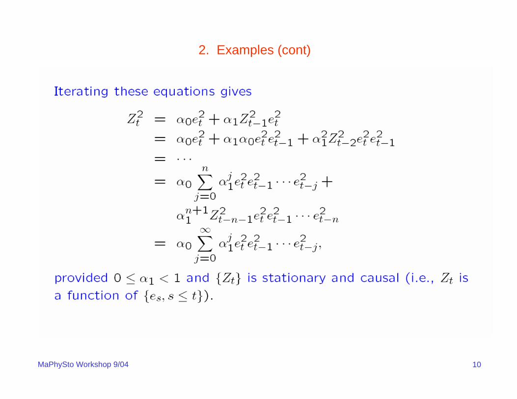
2. Examples (cont)

7MaPhySto Workshop 9/04
2. Examples (cont)

8MaPhySto Workshop 9/04
2. Examples (cont)

9MaPhySto Workshop 9/04
2. Examples (cont)
10MaPhySto Workshop 9/04
2. Examples (cont)

11MaPhySto Workshop 9/04
2. Examples (cont)

12MaPhySto Workshop 9/04
2. Examples (cont)
Properties of ARCH(1) process:
1. Strictly stationary solution if 0 < α1 <1.
2. {Zt} ~ WN(0,α0/(1-α1)).
3. Not IID since
4. Not Gaussian.
5. Zt has a symmetric distribution (Z1 =d – Z1)
6. EZt4 < ∞ if and only if 3α1
2 < 1. (More on moments later.)
7. If EZt4 < ∞, then the squared process Yt = Zt
2 has the same ACF as the AR(1) process
Wt = α1Wt-1 + et

13MaPhySto Workshop 9/04
2. Examples (cont)
Likelihood function:

14MaPhySto Workshop 9/04
2. Examples (cont)
A realization of the process

15MaPhySto Workshop 9/04
2. Examples (cont)
The sample ACF.

16MaPhySto Workshop 9/04
2. Examples (cont)
The sample ACF of the absolute values and squares.
17MaPhySto Workshop 9/04MaPhySto Workshop 9/04

18MaPhySto Workshop 9/04
Define Xt = 100*(ln (Pt) - ln (Pt-1)) (log returns)
• heavy tailed
P(|X1| > x) ~ C x-α, 0 < α < 4.
• uncorrelated
near 0 for all lags h > 0 (MGD sequence?)
• |Xt| and Xt2 have slowly decaying autocorrelations
converge to 0 slowly as h increases.
• process exhibits ‘stochastic volatility’.
)(ˆ hXρ
)(ˆ and )(ˆ 2|| hhXX ρρ
3. “Stylized Facts” of Financial Returns

19MaPhySto Workshop 9/04
1962 1967 1972 1977 1982 1987 1992 1997
time
-20
-10
010
100*
log(
retu
rns)
Log returns for IBM 1/3/62-11/3/00 (blue=1961-1981)
20MaPhySto Workshop 9/04
0 10 20 30 40
Lag
0.0
0.2
0.4
0.6
0.8
1.0
AC
F(a) ACF of IBM (1st half)
0 10 20 30 40
Lag
0.0
0.2
0.4
0.6
0.8
1.0
AC
F
(b) ACF of IBM (2nd half)
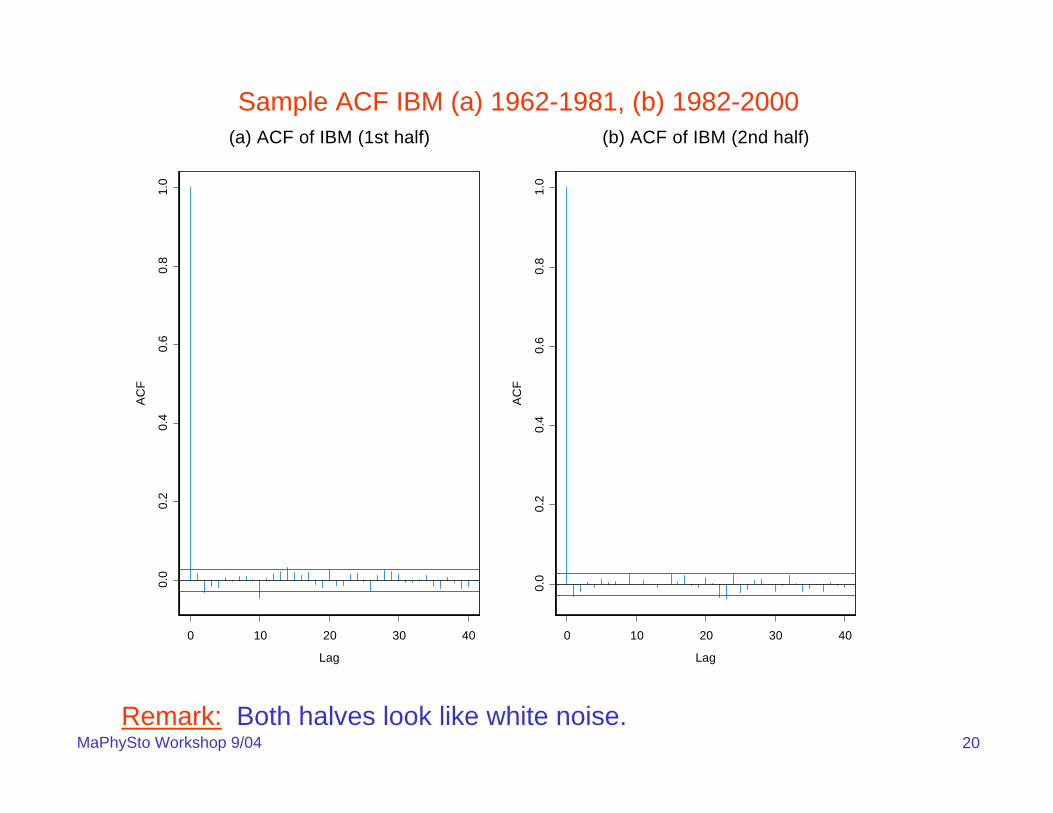
Sample ACF IBM (a) 1962-1981, (b) 1982-2000
Remark: Both halves look like white noise.
21MaPhySto Workshop 9/04
0 10 20 30 40
Lag
0.0
0.2
0.4
0.6
0.8
1.0
AC
F
(a) ACF, Squares of IBM (1st half)
0 10 20 30 40
Lag
0.0
0.2
0.4
0.6
0.8
1.0
AC
F
(b) ACF, Squares of IBM (2nd half)
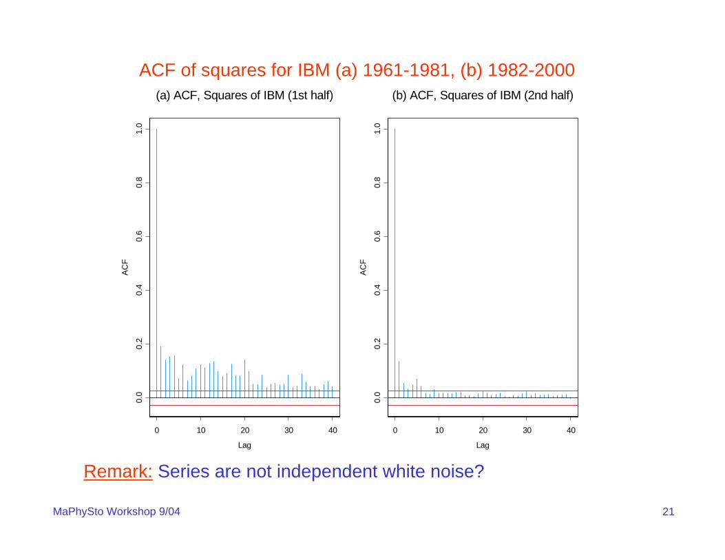
ACF of squares for IBM (a) 1961-1981, (b) 1982-2000
Remark: Series are not independent white noise?

22MaPhySto Workshop 9/04
0 2000 4000 6000 8000 10000
t
0.0
0.2
0.4
0.6
0.8
1.0
M(4
)/S(4
)
Plot of Mt(4)/St(4) for IBM
Remark: For IID data, Mt(k)/St(k) → 0 as t → ∞ iff E|X,|k < ∞, where
|| and ||max1
,...,1 ∑=
= ==t
s
kst
kstst XSXM

23MaPhySto Workshop 9/04
Hill’s estimator of tail indexThe marginal distribution F for heavy-tailed data is often modeled usingPareto-like tails,
1-F(x) = x-αL(x),
for x large, where L(x) is a slowly varying function (L(xt)/ L(x)→1, as x→∞). Now if
X~ F, then P(log X > x) = P(X > exp(x))=exp(-αx)L(exp(x)),
and hence log X has an approximate exponential distribution for large x. The spacings,
log( X(j)) − log(X(j+1)) , j=1,2,. . . ,m,
from a sample of size n from an exponential distr are approximately independent and ExpExp(αj) distributed. This suggests estimating α−1 by
( )
( )∑
∑
=+
=+
−
−=
−=α
m
jmj
m
jjj
XXm
jXXm
1)1()(
1)1()(
1
loglog1
loglog1ˆ

24MaPhySto Workshop 9/04
Hill’s estimator of tail index
Def: The Hill estimate of α for heavy-tailed data with distribution given by
1-F(x) = x-αL(x),
is
( )
( )∑
∑
=+
=+
−
−=
−=α
m
jmj
m
jjj
XXm
jXXm
1)1()(
1)1()(
1
loglog1
loglog1ˆ
The asymptotic variance of this estimate for α is
and estimated by
(See also GPD=generalized Pareto distribution.)
m/2α ./ˆ 2 mα

25MaPhySto Workshop 9/04
0 200 400 600 800 1000
m
12
34
5
Hill
0 200 400 600 800
m
12
34
5
Hill
Hill’s plot of tail index for IBM (1962-1981, 1982-2000)

26MaPhySto Workshop 9/04
4. ARCH and GARCH Models

27MaPhySto Workshop 9/04
4. ARCH and GARCH Models (cont)

28MaPhySto Workshop 9/04
4. ARCH and GARCH Models (cont)

29MaPhySto Workshop 9/04
4. ARCH and GARCH Models (cont)

30MaPhySto Workshop 9/04
4. ARCH and GARCH Models (cont)

31MaPhySto Workshop 9/04
4. ARCH and GARCH Models (cont)

32MaPhySto Workshop 9/04
4. ARCH and GARCH Models (cont)

33MaPhySto Workshop 9/04
4. ARCH and GARCH Models (cont)

34MaPhySto Workshop 9/04
4. ARCH and GARCH Models (cont)

35MaPhySto Workshop 9/04
4. ARCH and GARCH Models (cont)

36MaPhySto Workshop 9/04
4. ARCH and GARCH Models (cont)

37MaPhySto Workshop 9/04
4. ARCH and GARCH Models (cont)
i

38MaPhySto Workshop 9/04
4. ARCH and GARCH Models (cont)

39MaPhySto Workshop 9/04

40MaPhySto Workshop 9/04
4. ARCH and GARCH Models (cont)

41MaPhySto Workshop 9/04
4. ARCH and GARCH Models (cont)
SS but not WS GARCH Processes
MaPhySto Workshop 9/04

42MaPhySto Workshop 9/04
4. ARCH and GARCH Models (cont)

43MaPhySto Workshop 9/04

44MaPhySto Workshop 9/04
4. ARCH and GARCH Models (cont)
MaPhySto Workshop 9/04

45MaPhySto Workshop 9/04
4. ARCH and GARCH Models (cont)

46MaPhySto Workshop 9/04MaPhySto Workshop 9/04

47MaPhySto Workshop 9/04MaPhySto Workshop 9/04

48MaPhySto Workshop 9/04MaPhySto Workshop 9/04

49MaPhySto Workshop 9/04
Parameter Estimation for Finite-Variance GARCH Models

50MaPhySto Workshop 9/04
4. ARCH and GARCH Models (cont)

51MaPhySto Workshop 9/04MaPhySto Workshop 9/04

52MaPhySto Workshop 9/04

53MaPhySto Workshop 9/04
4. ARCH and GARCH Models (cont)

54MaPhySto Workshop 9/04
4. ARCH and GARCH Models (cont)

55MaPhySto Workshop 9/04
4. ARCH and GARCH Models (cont)

56MaPhySto Workshop 9/04
4. ARCH and GARCH Models (cont)

57MaPhySto Workshop 9/04
4. ARCH and GARCH Models (cont)

58MaPhySto Workshop 9/04
4. ARCH and GARCH Models (cont)

59MaPhySto Workshop 9/04
4. ARCH and GARCH Models (cont)

60MaPhySto Workshop 9/04
4. ARCH and GARCH Models (cont)

61MaPhySto Workshop 9/04
4. ARCH and GARCH Models (cont)

62MaPhySto Workshop 9/04
4. ARCH and GARCH Models (cont)
MaPhySto Workshop 9/04

63MaPhySto Workshop 9/04MaPhySto Workshop 9/04

64MaPhySto Workshop 9/04
4. ARCH and GARCH Models (cont)

65MaPhySto Workshop 9/04
4. ARCH and GARCH Models (cont)

66MaPhySto Workshop 9/04
5. Forecasting with GARCH

67MaPhySto Workshop 9/04
5. Forecasting with GARCH (cont)

68MaPhySto Workshop 9/04
6. IGARCH

69MaPhySto Workshop 9/04
7. Stochastic Volatility Models

70MaPhySto Workshop 9/04
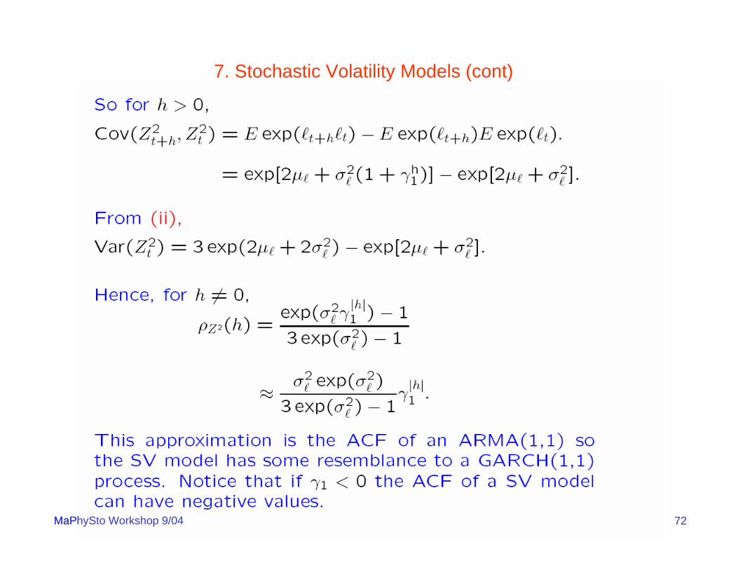
7. Stochastic Volatility Models (cont)

71MaPhySto Workshop 9/04
7. Stochastic Volatility Models (cont)
72MaPhySto Workshop 9/04
7. Stochastic Volatility Models (cont)
MaPhySto Workshop 9/04

73MaPhySto Workshop 9/04
7. Stochastic Volatility Models (cont)
MaPhySto Workshop 9/04

74MaPhySto Workshop 9/04
7. Stochastic Volatility Models (cont)

75MaPhySto Workshop 9/04
7. Stochastic Volatility Models (cont)

76MaPhySto Workshop 9/04
7. Stochastic Volatility Models (cont)

77MaPhySto Workshop 9/04
7. Stochastic Volatility Models (cont)

78MaPhySto Workshop 9/04
7. Stochastic Volatility Models (cont)

79MaPhySto Workshop 9/04
7. Stochastic Volatility Models (cont)

80MaPhySto Workshop 9/04
7. Stochastic Volatility Models (cont)

81MaPhySto Workshop 9/04
82MaPhySto Workshop 9/04
7. Stochastic Volatility Models (cont)

83MaPhySto Workshop 9/04
8. Regular variation and application to financial TS models
8.1 Regular variation — univariate case
Def: The random variable X is regularly varying with index α if
P(|X|> t x)/P(|X|>t) → x−α and P(X> t)/P(|X|>t) →p,
or, equivalently, if
P(X> t x)/P(|X|>t) → px−α and P(X< −t x)/P(|X|>t) → qx−α ,
where 0 ≤ p ≤ 1 and p+q=1.Equivalence:
X is RV(α) if and only if P(X ∈ t • ) /P(|X|>t)→v µ(• )
(→v vague convergence of measures on RR\{0}). In this case,
µ(dx) = (pα x−α−1 I(x>0) + qα (-x)-α−1 I(x<0)) dx
Note: µ(tA) = t-α µ(A) for every t and A bounded away from 0.

84MaPhySto Workshop 9/04
Another formulation (polar coordinates):
Define the ± 1 valued rv θ, P(θ = 1) = p, P(θ = −1) = 1− p = q.Then
X is RV(α) if and only if
or
(→v vague convergence of measures on SS0= {-1,1}).
)(x)t |X(|
)|X|X/ t x, |X(| SPP
SP∈→
>∈> α− θ
)(x)t |X(|
)|X|X/ t x, |X(|•∈→
>•∈> α− θP
PP
v
8.1 Regular variation — univariate case (cont)

85MaPhySto Workshop 9/04
Equivalence:
µ is a measure on RRm which satisfies for x > 0 and A bounded away from 0,
µ(xB) = x−α µ(xA).
Multivariate regular variation of X=(X1, . . . , Xm): There exists a random vector θ ∈ Sm-1 such that
P(|X|> t x, X/|X| ∈ • )/P(|X|>t) →v x−α P( θ ∈ • )
(→v vague convergence on SSm-1, unit sphere in Rm) .
• P( θ ∈•) is called the spectral measure
• α is the index of X.
)()t |(|)t (
•µ→>
•∈vP
PXX )(
)t |(|)t (
•µ→>
•∈vP
PXX
8.2 Regular variation — multivariate case

86MaPhySto Workshop 9/04
1. If X1> 0 and X2 > 0 are iid RV(α), then X= (X1, X2 ) is multivariate regularly varying with index α and spectral distribution
P( θ =(0,1) ) = P( θ =(1,0) ) =.5 (mass on axes).
Interpretation: Unlikely that X1 and X2 are very large at the same time.
0 5 10 15 20
x_1
010
2030
40x_
2Figure: plot of (Xt1,Xt2) for realization of 10,000.
8.2 Regular variation — multivariate case (cont)Examples:

87MaPhySto Workshop 9/04
2. If X1 = X2 > 0, then X= (X1, X2 ) is multivariate regularly varying with index α and spectral distribution
P( θ = (1/√2, 1/√2) ) = 1.
3. AR(1): Xt= .9 Xt-1 + Zt , {Zt}~IID symmetric stable (1.8)
±(1,.9)/sqrt(1.81), W.P. .9898
±(0,1), W.P. .0102{
-10 0 10 20 30x_t
-10
010
2030
x_{t+
1}
Figure: plot of (Xt, Xt+1) for realization of 10,000.
Distr of θ:

88MaPhySto Workshop 9/04
• Domain of attraction for sums of iid random vectors(Rvaceva, 1962). That is, when does the partial sum
converge for some constants an?
• Spectral measure of multivariate stable vectors.
• Domain of attraction for componentwise maxima of iidrandom vectors (Resnick, 1987). Limit behavior of
• Weak convergence of point processes with iid points.
• Solution to stochastic recurrence equations, Y t= At Yt-1 + Bt
• Weak convergence of sample autocovariances.
∑=
−n
tna
1t
1 X
t1
1 Xn
tna=
− ∨
8.3 Applications of multivariate regular variation

89MaPhySto Workshop 9/04
Use vague convergence with Ac={y: cTy > 1}, i.e.,
where t-αL(t) = P(|X| > t).
Linear combinations:
X ~RV(α) ⇒ all linear combinations of X are regularly varying
),(w:)A()t |(|)t (
)()tA ( T
cXXcX
cc =µ→
>>
=∈
α− PP
tLtP
i.e., there exist α and slowly varying fcn L(.), s.t.
P(cTX> t)/(t-αL(t)) →w(c), exists for all real-valued c,
where
w(tc) = t−αw(c).
Ac),(w:)A()t |(|)t (
)()tA ( T
cXXcX
cc =µ→
>>
=∈
α− PP
tLtP
8.3 Applications of multivariate regular variation (cont)

90MaPhySto Workshop 9/04
Converse?
X ~RV(α) ⇐ all linear combinations of X are regularly varying?
There exist α and slowly varying fcn L(.), s.t.
(LC) P(cTX> t)/(t-αL(t)) →w(c), exists for all real-valued c.
Theorem (Basrak, Davis, Mikosch, `02). Let X be a random vector.
1. If X satisfies (LC) with α non-integer, then X is RV(α).
2. If X > 0 satisfies (LC) for non-negative c and α is non-integer,
then X is RV(α).
3. If X > 0 satisfies (LC) with α an odd integer, then X is RV(α).
8.3 Applications of multivariate regular variation (cont)

91MaPhySto Workshop 9/04
1. Kesten (1973). Under general conditions, (LC) holds with L(t)=1
for stochastic recurrence equations of the form
Yt= At Yt-1+ Bt, (At , Bt) ~ IID,
At d×d random matrices, Bt random d-vectors.
It follows that the distributions of Yt, and in fact all of the finite dim’l
distrs of Yt are regularly varying (if α is non-even).
2. GARCH processes. Since squares of a GARCH process can be
embedded in a SRE, the finite dimensional distributions of a
GARCH are regularly varying.
8.4 Applications of theorem

92MaPhySto Workshop 9/04
Example of ARCH(1): Xt=(α0+α1 X2t-1)1/2Zt, {Zt}~IID.
α found by solving E|α1 Z2|α/2 = 1.
α1 .312 .577 1.00 1.57α 8.00 4.00 2.00 1.00
Distr of θ:
P(θ ∈ •) = E{||(B,Z)||α I(arg((B,Z)) ∈ •)}/ E||(B,Z)||α
where
P(B = 1) = P(B = -1) =.5
8.5 Examples

93MaPhySto Workshop 9/04
Figures: plots of (Xt, Xt+1) and estimated distribution of θ for realization of 10,000.
Example of ARCH(1): α0=1, α1=1, α=2, Xt=(α0+α1 X2t-1)1/2Zt, {Zt}~IID
-20 -10 0 10 20
x_t
-20
-10
010
20x_
{t+1}
-3 -2 -1 0 1 2 3
theta
0.06
0.08
0.10
0.12
0.14
0.16
0.18
8.4 Examples (cont)

94MaPhySto Workshop 9/04
Example: SV model Xt = σt Zt
Suppose Zt ~ RV(α) and
Then Zn=(Z1,…,Zn)’ is regulary varying with index α and so is
Xn= (X1,…,Xn)’ = diag(σ1,…, σn) Zn
with spectral distribution concentrated on (±1,0), (0, ±1).
).N(0, IID~}{ , ,log 222 σε∞<ψεψ=σ ∑∑∞
−∞=−
∞
−∞=t
jjjt
jjt
-5000 0 5000 10000
x_1
-500
00
5000
1000
0x_
2
Figure: plot of (Xt,Xt+1) for realization of 10,000.
8.4 Applications of theorem (cont)

95MaPhySto Workshop 9/04
Setup
Xt = σt Zt , {Zt} ~ IID (0,1)
Xt is RV (α)
Choose {bn} s.t. nP(Xt > bn) →1
Then }.exp{)( 1
1 α−− −→≤ xxXbP nn
Then, with Mn= max{X1, . . . , Xn},
(i) GARCH:
γ is extremal index ( 0 < γ < 1).
(ii) SV model:
extremal index γ = 1 no clustering.
},exp{)( 1 α−− γ−→≤ xxMbP nn
},exp{)( 1 α−− −→≤ xxMbP nn
8.6 Extremes for GARCH and SV processes

96MaPhySto Workshop 9/04
(i) GARCH:
(ii) SV model:
}exp{)( 1 α−− γ−→≤ xxMbP nn
}exp{)( 1 α−− −→≤ xxMbP nn
Remarks about extremal index.
(i) γ < 1 implies clustering of exceedances
(ii) Numerical example. Suppose c is a threshold such that
Then, if γ = .5,
(iii) 1/γ is the mean cluster size of exceedances.
(iv) Use γ to discriminate between GARCH and SV models.
(v) Even for the light-tailed SV model (i.e., {Zt} ~IID N(0,1), the extremal index is 1 (see Breidt and Davis `98 )
95.~)( 11 cXbP n
n ≤−
975.)95(.~)( 5.1 =≤− cMbP nn
8.6 Extremes for GARCH and SV processes (cont)

97MaPhySto Workshop 9/04
0 20 40 60
time
010
2030
0 20 40 60
time
010
2030
** * * *** ***
8.6 Extremes for GARCH and SV processes (cont)

98MaPhySto Workshop 9/04
α∈(0,2):
α∈(2,4):
α∈(4,∞):
Remark: Similar results hold for the sample ACF based on |Xt| andXt
2.
,)/())(ˆ( ,,10,,1 mhhd
mhX VVh KK == ⎯→⎯ρ
( ) ( ) .)0()(ˆ ,,11
,,1/21
mhhXd
mhX VhnKK =
−=
α− γ⎯→⎯ρ
( ) ( ) .)0()(ˆ ,,11
,,12/1
mhhXd
mhX GhnKK =
−= γ⎯→⎯ρ
8.7 Summary of results for ACF of GARCH(p,q) and SV models
GARCH(p,q)

99MaPhySto Workshop 9/04
α∈(0,2):
α∈(2, ∞):
( ) ( ) .)0()(ˆ ,,11
,,12/1
mhhXd
mhX GhnKK =
−= γ⎯→⎯ρ
( ) .)(ˆln/0
21
1h1/1
SShnn hd
X
α
α+α
σ
σσ⎯→⎯ρ
8.7 Summary of results for ACF of GARCH(p,q) and SV models (cont)
SV Model

100MaPhySto Workshop 9/04
Sample ACF for GARCH and SV Models (1000 reps)
-0.3
-0.1
0.1
0.3
(a) GARCH(1,1) Model, n=10000-0
.06
-0.0
20.
02
(b) SV Model, n=10000

101MaPhySto Workshop 9/04
Sample ACF for Squares of GARCH (1000 reps)
(a) GARCH(1,1) Model, n=100000.
00.
20.
40.
60.
00.
20.
40.
6
b) GARCH(1,1) Model, n=100000

102MaPhySto Workshop 9/04
Sample ACF for Squares of SV (1000 reps)0.
00.
010.
020.
030.
04
(d) SV Model, n=100000
0.0
0.05
0.10
0.15
(c) SV Model, n=10000

103MaPhySto Workshop 9/04
-1.00
-.80
-.60
-.40
-.20
.00
.20
.40
0 400 800 1200 1600
Series
Example: Amazon returns May 16, 1997 to June 16, 2004.
-1.00
-.80
-.60
-.40
-.20
.00
.20
.40
.60
.80
1.00
0 5 10 15 20 25 30 35 40
Residual ACF: Abs values
-1.00
-.80
-.60
-.40
-.20
.00
.20
.40
.60
.80
1.00
0 5 10 15 20 25 30 35 40
Residual ACF: Squares

104MaPhySto Workshop 9/04
Wrap-up
• Regular variation is a flexible tool for modeling both dependence
and tail heaviness.
• Useful for establishing point process convergence of heavy-tailed
time series.
• Extremal index γ < 1 for GARCH and γ =1 for SV.
Unresolved issues related to RV⇔ (LC)
• α = 2n?
• there is an example for which X1, X2 > 0, and (c, X1) and (c, X2)have the same limits for all c > 0.
• α = 2n−1 and X > 0 (not true in general).