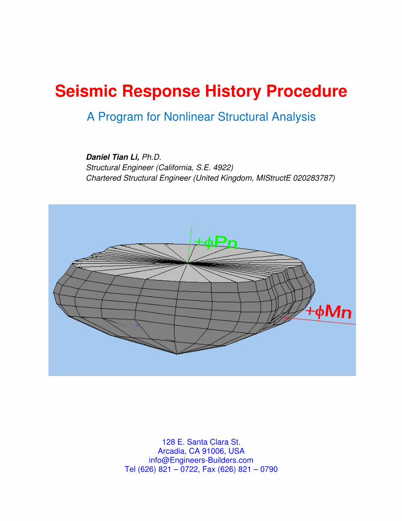
Seismic Response History Procedure

A Program for Nonlinear Structural Analysis

Daniel Tian Li, Ph.D.

Structural Engineer (California, S.E. 4922)

Chartered Structural Engineer (United Kingdom, MIStructE 020283787)

128 E. Santa Clara St.

Arcadia, CA 91006, USA info@Engineers-Builders.com

Tel (626) 821 – 0722, Fax (626) 821 – 0790

1. Introduction

The Seismic Response History Procedure (SRHP) is a determined nonlinear structural

analysis software, based on the most current IBC/CBC, ASCE, ACI and AASHTO,

without probability and/or fuzzy math. The SRHP is also an open system, which the

element matrix, design criteria, and even nonlinear method, are all changeable. From

the manual example, user can find a 5 story building, under El Centro 1940 earthquake,

history procedures of story drift, equivalent base shear and later forces, and their

maximum value with its happened time.

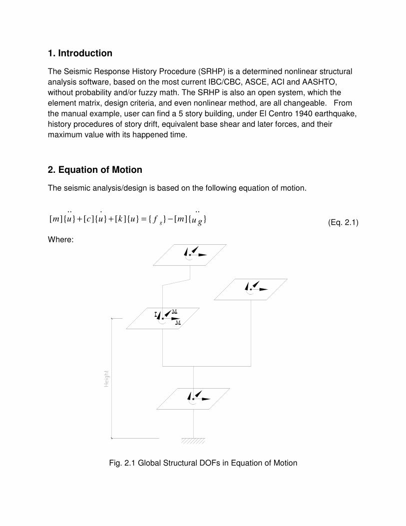
2. Equation of Motion

The seismic analysis/design is based on the following equation of motion.

(Eq. 2.1)

Where:

Fig. 2.1 Global Structural DOFs in Equation of Motion

.. . ..[ ] [ ] [ ] [ ]

gm u c u k u mf u g+ + = −

[m] = Diagonal mass matrix based on each floor diaphragm center points (selected

global DOFs), including horizontal X, Y directions, and Φ moment of inertia. The

each floor diaphragm center points may not be at a same vertical location to keep

mass matrix diagonal.

The moment of inertia is a rigid diaphragm concept. Semirigid modeling

assumption (ASCE 7-10 12.3.1) forces the [m] to non-diagonal matrix, which

results from Complex Eigenvector modes. This software user can cut a diaphragm

to two and more, but each smaller one has to be rigid.

u = Displacement vector at each floor diaphragm center points, including horizontal X,

Y directions, and Φ rotation. Typical for velocity ù and acceleration ȕ.

[k] = Lateral stiffness full matrix based on each floor diaphragm center points, which

concentrated from each vertical 2D frames.

ȕg = Ground acceleration, including horizontal X, Y directions, and Φ rotation, without

SRSS probability issue. User can rotate the structural locations to get maximum

responses.

To get the ground motions in a maximum direction (ASCE 7-10 16.1.3.2) is

based on Single Degree of Freedom, because any actual structural stiffness, [k],

is full matrix, which means that the two horizontal X and Y responses coupled

together. One of DOFs at one direction reached maximum response does not

mean other all DOFs maximum responses, even minimum at the same direction.

[c] = Damping matrix as follows.

(Eq. 2.2)

The reasons that Eq. 2.2 has to be applied are

1. Only damping ratio of ζ has been called out, 5%, on ASCE 7-10, 16.1.3 &

21.1.3. There are no other adapted law document for damping input. The

(Eq. 2.2) has reached the code requirement.

2. The (Eq. 2.2) is an applicable math method to solve the equation of

motion(Eq. 2.1), because structural period T1 & T2 are not constants in

nonlinear structural analysis. The T1 & T2 are changed in each time steps

after plastic hinges formed.

fg = Must be Zero vector. Otherwise, the equation (Eq. 2.1) cannot be solved as

classical damped system. The static gravity loads are not vectors changed on

time steps in Equation of Motion.

( ) ( )( )

1 2

1 2 1 2

4[ ] [ ] [ ]

T Tc m k

T T T T

π ξ ξ

π= +

+ +

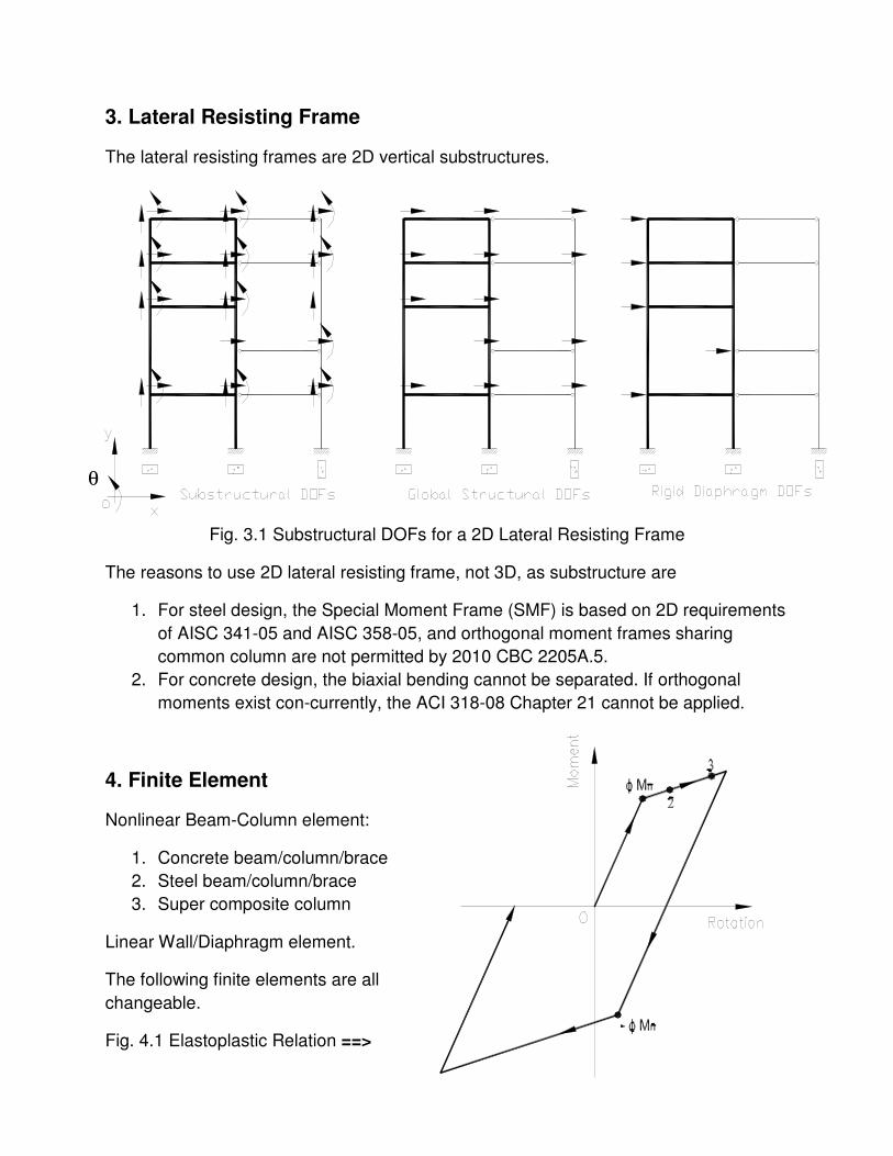
3. Lateral Resisting Frame

The lateral resisting frames are 2D vertical substructures.

Fig. 3.1 Substructural DOFs for a 2D Lateral Resisting Frame

The reasons to use 2D lateral resisting frame, not 3D, as substructure are

1. For steel design, the Special Moment Frame (SMF) is based on 2D requirements

of AISC 341-05 and AISC 358-05, and orthogonal moment frames sharing

common column are not permitted by 2010 CBC 2205A.5.

2. For concrete design, the biaxial bending cannot be separated. If orthogonal

moments exist con-currently, the ACI 318-08 Chapter 21 cannot be applied.

4. Finite Element

Nonlinear Beam-Column element:

1. Concrete beam/column/brace

2. Steel beam/column/brace

3. Super composite column

Linear Wall/Diaphragm element.

The following finite elements are all

changeable.

Fig. 4.1 Elastoplastic Relation ==>

θ

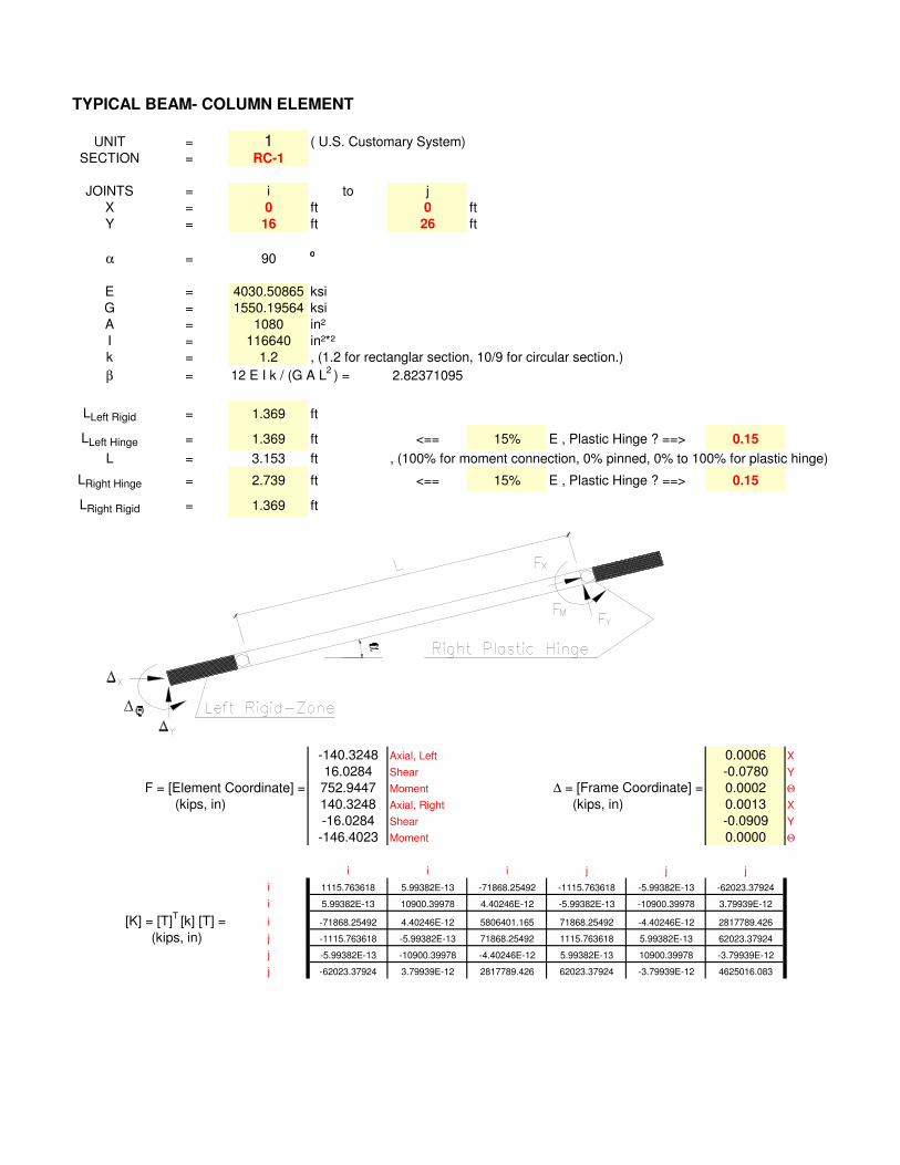
TYPICAL BEAM- COLUMN ELEMENT

UNIT = 1 ( U.S. Customary System)

SECTION = RC-1

JOINTS = i to j

X = 0 ft 0 ft

Y = 16 ft 26 ft

α = 90o

E = 4030.50865 ksi

G = 1550.19564 ksi

A = 1080 in²

I = 116640 in²*²

k = 1.2 , (1.2 for rectanglar section, 10/9 for circular section.)

β = 12 E I k / (G A L2 ) = 2.82371095

LLeft Rigid = 1.369 ft

LLeft Hinge = 1.369 ft <== 15% E , Plastic Hinge ? ==> 0.15

L = 3.153 ft , (100% for moment connection, 0% pinned, 0% to 100% for plastic hinge)

LRight Hinge = 2.739 ft <== 15% E , Plastic Hinge ? ==> 0.15

LRight Rigid = 1.369 ft

-140.3248 Axial, Left 0.0006 X

16.0284 Shear -0.0780 Y

752.9447 Moment ∆ = [Frame Coordinate] = 0.0002 Θ

(kips, in) 140.3248 Axial, Right (kips, in) 0.0013 X

-16.0284 Shear -0.0909 Y

-146.4023 Moment 0.0000 Θ

i i i j j j

i 1115.763618 5.99382E-13 -71868.25492 -1115.763618 -5.99382E-13 -62023.37924

i 5.99382E-13 10900.39978 4.40246E-12 -5.99382E-13 -10900.39978 3.79939E-12

[K] = [T]T

[k] [T] = i -71868.25492 4.40246E-12 5806401.165 71868.25492 -4.40246E-12 2817789.426

(kips, in) j -1115.763618 -5.99382E-13 71868.25492 1115.763618 5.99382E-13 62023.37924

j -5.99382E-13 -10900.39978 -4.40246E-12 5.99382E-13 10900.39978 -3.79939E-12

j -62023.37924 3.79939E-12 2817789.426 62023.37924 -3.79939E-12 4625016.083

F = [Element Coordinate] =

Section RC-1

No. 1

INPUT DATA & DESIGN SUMMARY

CONCRETE STRENGTH fc' = 5 ksi

REBAR YIELD STRESS fy = 60 ksi

SECTION SIZE Cx = 36 in

Cy = 30

FACTORED AXIAL LOAD Pu = 300 k

FACTORED MAGNIFIED MOMENT Mu = 840.9 ft-k

VERT. REINFORCEMENT 7 # 9 at x dir.

3 # 9 at y dir.

LATERAL FRAME DIRECTION θ = 0 deg

Linear Stage

ANALYSIS

φ Pn (k)

φ Mn (ft-k)

φ φ φ φ Pn (k) φφφφ Mn (ft-k)

AT AXIAL LOAD ONLY 2967 0

AT MAXIMUM LOAD 2967 790

AT 0 % TENSION 2570 1131

AT 25 % TENSION 2159 1390

AT 50 % TENSION 1830 1532

AT ε t = 0.002 1342 1674

AT BALANCED CONDITION 1323 1695

AT ε t = 0.005 866 2074

AT FLEXURE ONLY 0 1276

AT PURE TENSION -1080 0

(Total 20 # 9)

in

Concrete Section Design Based on ACI 318-08

-1500

-1000

-500

0

500

1000

1500

2000

2500

3000

3500

0 500 1000 1500 2000 2500

( )'

'

2

'

'

2 0.85, 57 , 29000

0.85 2 , 0

0.85 ,

,

,

C

C

C

C

C

S

fksifE Ec so

Ec

c c forf c of oo

forf c o

forEss s tf

forf s ty

ε

ε εε ε

εε

ε ε

ε ε ε

ε ε

= = =

− < <

=

≥

≤= >

ε

ε

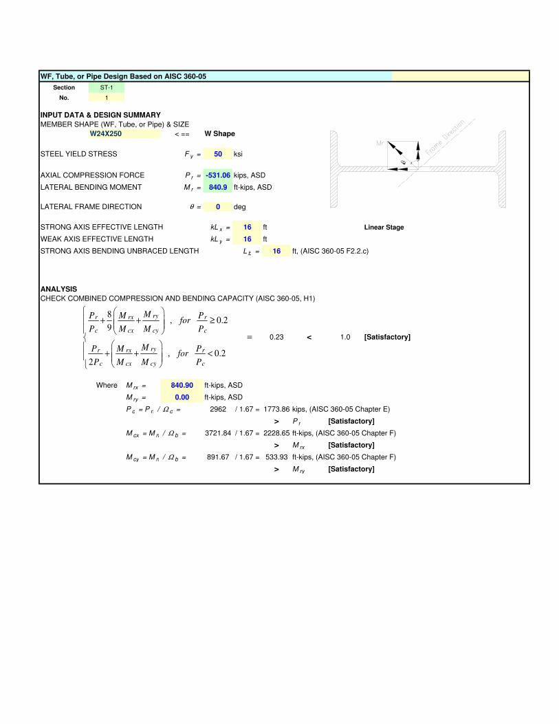
Section ST-1

No. 1

INPUT DATA & DESIGN SUMMARY

MEMBER SHAPE (WF, Tube, or Pipe) & SIZE

W24X250 < == W Shape

STEEL YIELD STRESS F y = 50 ksi

AXIAL COMPRESSION FORCE P r = -531.06 kips, ASD

LATERAL BENDING MOMENT M r = 840.9 ft-kips, ASD

LATERAL FRAME DIRECTION θ = 0 deg

STRONG AXIS EFFECTIVE LENGTH kL x = 16 ft Linear Stage

WEAK AXIS EFFECTIVE LENGTH kL y = 16 ft

STRONG AXIS BENDING UNBRACED LENGTH L b = 16 ft, (AISC 360-05 F2.2.c)

ANALYSIS

CHECK COMBINED COMPRESSION AND BENDING CAPACITY (AISC 360-05, H1)

0.23 < 1.0 [Satisfactory]

Where M rx = 840.90 ft-kips, ASD

M ry = 0.00 ft-kips, ASD

P c = P n / Ω c = 2962 / 1.67 = 1773.86 kips, (AISC 360-05 Chapter E)

> P r [Satisfactory]

M cx = M n / Ω b = 3721.84 / 1.67 = 2228.65 ft-kips, (AISC 360-05 Chapter F)

> M rx [Satisfactory]

M cy = M n / Ω b = 891.67 / 1.67 = 533.93 ft-kips, (AISC 360-05 Chapter F)

> M ry [Satisfactory]

WF, Tube, or Pipe Design Based on AISC 360-05

8, 0.2

9

, 0.22

ryr rx r

c cx cy c

ryr rx r

c cx cy c

MP M Pfor

P M M P

MP M Pfor

P M M P

+ + ≥

=

+ + <

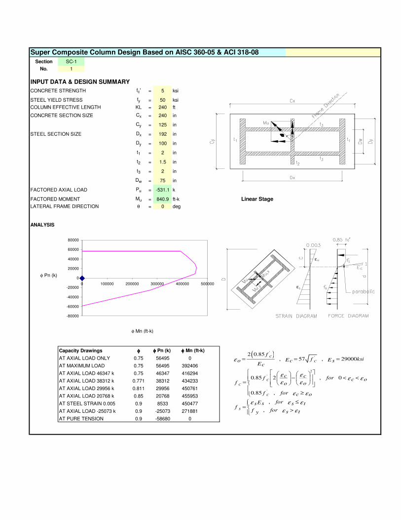
Section SC-1

No. 1

INPUT DATA & DESIGN SUMMARY

CONCRETE STRENGTH fc' = 5 ksi

STEEL YIELD STRESS fy = 50 ksi

COLUMN EFFECTIVE LENGTH KL = 240 ft

CONCRETE SECTION SIZE Cx = 240 in

Cy = 125

STEEL SECTION SIZE Dx = 192

Dy = 100

t1 = 2

t2 = 1.5

t3 = 2

Dw = 75

FACTORED AXIAL LOAD Pu = -531.1 k

FACTORED MOMENT Mu = 840.9 ft-k Linear Stage

LATERAL FRAME DIRECTION θ = 0 deg

ANALYSIS

φ Pn (k)

φ Mn (ft-k)

Capacity Drawings φφφφ φ φ φ φ Pn (k) φφφφ Mn (ft-k)

AT AXIAL LOAD ONLY 0.75 56495 0

AT MAXIMUM LOAD 0.75 56495 392406

AT AXIAL LOAD 46347 k 0.75 46347 416294

AT AXIAL LOAD 38312 k 0.771 38312 434233

AT AXIAL LOAD 29956 k 0.811 29956 450761

AT AXIAL LOAD 20768 k 0.85 20768 455953

AT STEEL STRAIN 0.005 0.9 8533 450477

AT AXIAL LOAD -25073 k 0.9 -25073 271881

AT PURE TENSION 0.9 -58680 0

in

Super Composite Column Design Based on AISC 360-05 & ACI 318-08

in

in

in

in

in

in

-80000

-60000

-40000

-20000

0

20000

40000

60000

80000

0 100000 200000 300000 400000 500000

( )'

'

2

'

'

2 0.85, 57 , 29000

0.85 2 , 0

0.85 ,

,

,

C

C

C

C

C

S

fksifE Ec so

Ec

c c forf c of oo

forf c o

forEss s tf

forf s ty

ε

ε εε ε

εε

ε ε

ε ε ε

ε ε

= = =

− < <

=

≥

≤= >

ε

ε

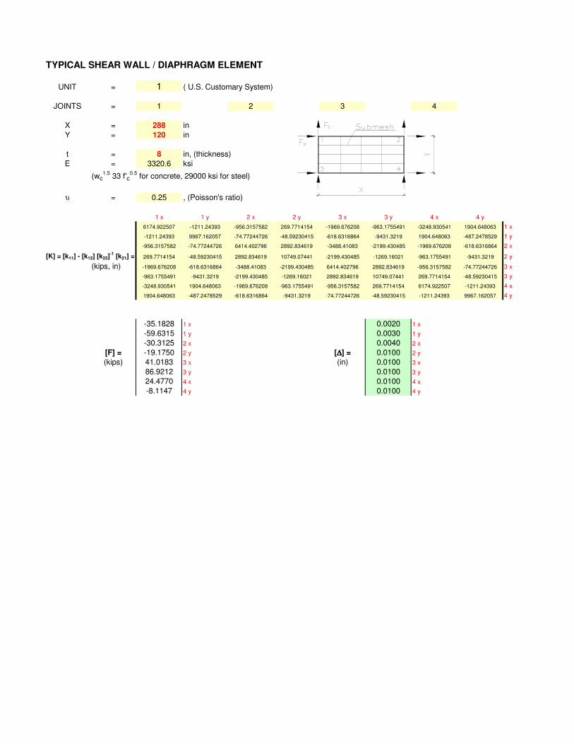
TYPICAL SHEAR WALL / DIAPHRAGM ELEMENT

UNIT = 1 ( U.S. Customary System)

JOINTS = 1 2 3 4

X = 288 in

Y = 120 in

t = 8 in, (thickness)

E = 3320.6 ksi

(wc1.5

33 f'c0.5

for concrete, 29000 ksi for steel)

υ = 0.25 , (Poisson's ratio)

1 x 1 y 2 x 2 y 3 x 3 y 4 x 4 y

6174.922507 -1211.24393 -956.3157582 269.7714154 -1969.676208 -963.1755491 -3248.930541 1904.648063 1 x

-1211.24393 9967.162057 -74.77244726 -48.59230415 -618.6316864 -9431.3219 1904.648063 -487.2478529 1 y

-956.3157582 -74.77244726 6414.402796 2892.834619 -3488.41083 -2199.430485 -1969.676208 -618.6316864 2 x

269.7714154 -48.59230415 2892.834619 10749.07441 -2199.430485 -1269.16021 -963.1755491 -9431.3219 2 y

(kips, in) -1969.676208 -618.6316864 -3488.41083 -2199.430485 6414.402796 2892.834619 -956.3157582 -74.77244726 3 x

-963.1755491 -9431.3219 -2199.430485 -1269.16021 2892.834619 10749.07441 269.7714154 -48.59230415 3 y

-3248.930541 1904.648063 -1969.676208 -963.1755491 -956.3157582 269.7714154 6174.922507 -1211.24393 4 x

1904.648063 -487.2478529 -618.6316864 -9431.3219 -74.77244726 -48.59230415 -1211.24393 9967.162057 4 y

-35.1828 1 x 0.0020 1 x

-59.6315 1 y 0.0030 1 y

-30.3125 2 x 0.0040 2 x

[F] = -19.1750 2 y [∆∆∆∆] = 0.0100 2 y

(kips) 41.0183 3 x (in) 0.0100 3 x

86.9212 3 y 0.0100 3 y

24.4770 4 x 0.0100 4 x

-8.1147 4 y 0.0100 4 y

[K] = [k11] - [k12] [k22]-1

[k21] =

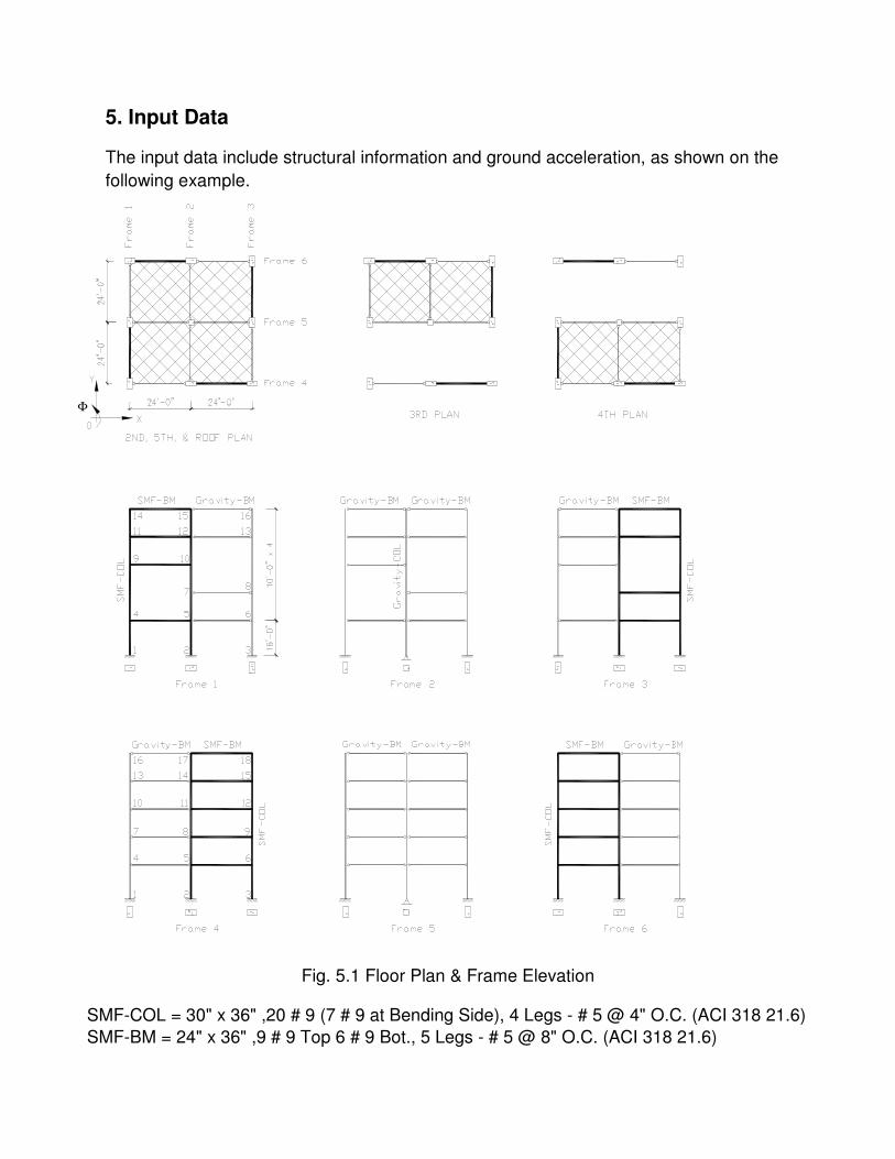
5. Input Data

The input data include structural information and ground acceleration, as shown on the

following example.

Fig. 5.1 Floor Plan & Frame Elevation

SMF-COL = 30" x 36" ,20 # 9 (7 # 9 at Bending Side), 4 Legs - # 5 @ 4" O.C. (ACI 318 21.6)

SMF-BM = 24" x 36" ,9 # 9 Top 6 # 9 Bot., 5 Legs - # 5 @ 8" O.C. (ACI 318 21.6)

Φ

Gravity-COL = 24" x 24" ,12 # 8, 4 Legs - # 4 @ 12" O.C., Continued as Built. Gravity-BM = 20" x 24" ,4 # 8 Bot., 4 Legs - # 4 @ 12" O.C., Pinned both Ends.

fc' = 5 ksi fy = 60 ksi Mass & Moment of Inertia per 0.125 kips/ft2

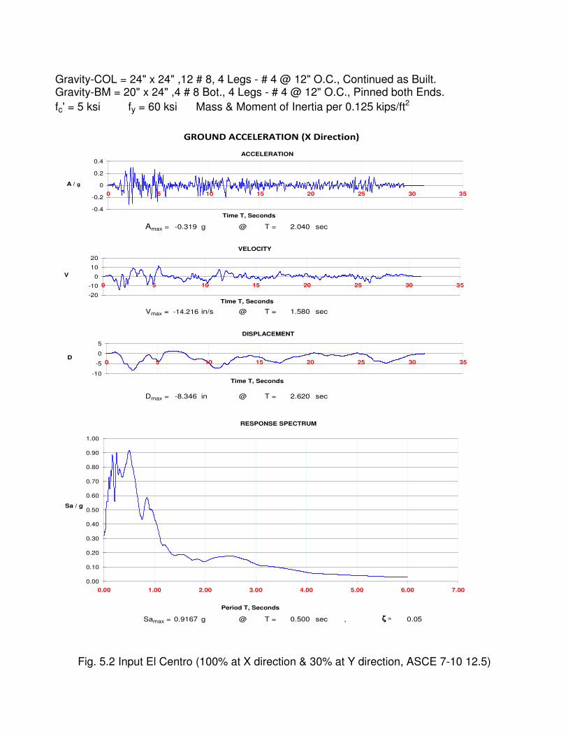
Fig. 5.2 Input El Centro (100% at X direction & 30% at Y direction, ASCE 7-10 12.5)

GROUND ACCELERATION (X Direction)

Amax = -0.319 g @ T = 2.040 sec

Vmax = -14.216 in/s @ T = 1.580 sec

Dmax = -8.346 in @ T = 2.620 sec

Samax = 0.9167 g @ T = 0.500 sec , ζζζζ = 0.05

ACCELERATION

-0.4

-0.2

0

0.2

0.4

0 5 10 15 20 25 30 35

Time T, Seconds

A / g

VELOCITY

-20

-10

0

10

20

0 5 10 15 20 25 30 35

Time T, Seconds

V

DISPLACEMENT

-10

-5

0

5

0 5 10 15 20 25 30 35

Time T, Seconds

D

RESPONSE SPECTRUM

0.00

0.10

0.20

0.30

0.40

0.50

0.60

0.70

0.80

0.90

1.00

0.00 1.00 2.00 3.00 4.00 5.00 6.00 7.00

Period T, Seconds

Sa / g

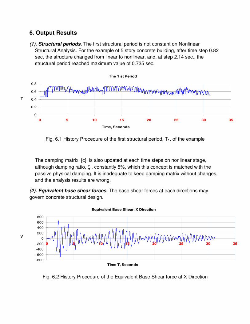
6. Output Results

(1). Structural periods. The first structural period is not constant on Nonlinear

Structural Analysis. For the example of 5 story concrete building, after time step 0.82

sec, the structure changed from linear to nonlinear, and, at step 2.14 sec., the

structural period reached maximum value of 0.735 sec.

Fig. 6.1 History Procedure of the first structural period, T1, of the example

The damping matrix, [c], is also updated at each time steps on nonlinear stage,

although damping ratio, ζ , constantly 5%, which this concept is matched with the

passive physical damping. It is inadequate to keep damping matrix without changes,

and the analysis results are wrong.

(2). Equivalent base shear forces. The base shear forces at each directions may

govern concrete structural design.

Fig. 6.2 History Procedure of the Equivalent Base Shear force at X Direction

The 1 st Period

0

0.2

0.4

0.6

0.8

0 5 10 15 20 25 30 35

Time, Seconds

T

Equivalent Base Shear, X Direction

-800

-600

-400

-200

0

200

400

600

800

0 5 10 15 20 25 30 35

Time T, Seconds

V

The maximum X direction base shear force is 692.3 kips (0.601 W) at time step 2.48

sec., which is larger than the load, 144 kips, by Equivalent Lateral Force Procedure

(ASCE 7-10 12.8).

(3). Story drifts. The story drift at each level and each direction always govern steel

structural design.

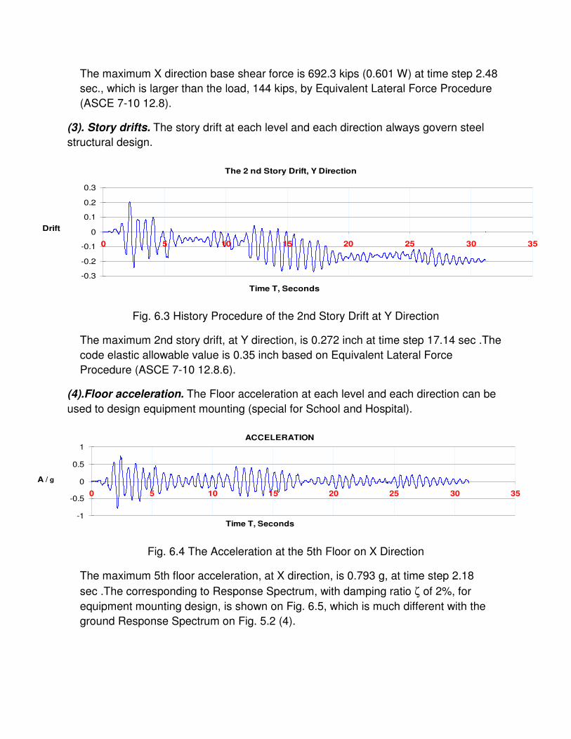
Fig. 6.3 History Procedure of the 2nd Story Drift at Y Direction

The maximum 2nd story drift, at Y direction, is 0.272 inch at time step 17.14 sec .The

code elastic allowable value is 0.35 inch based on Equivalent Lateral Force

Procedure (ASCE 7-10 12.8.6).

(4).Floor acceleration. The Floor acceleration at each level and each direction can be

used to design equipment mounting (special for School and Hospital).

Fig. 6.4 The Acceleration at the 5th Floor on X Direction

The maximum 5th floor acceleration, at X direction, is 0.793 g, at time step 2.18

sec .The corresponding to Response Spectrum, with damping ratio ζ of 2%, for

equipment mounting design, is shown on Fig. 6.5, which is much different with the

ground Response Spectrum on Fig. 5.2 (4).

The 2 nd Story Drift, Y Direction

-0.3

-0.2

-0.1

0

0.1

0.2

0.3

0 5 10 15 20 25 30 35

Time T, Seconds

Drift

ACCELERATION

-1

-0.5

0

0.5

1

0 5 10 15 20 25 30 35

Time T, Seconds

A / g

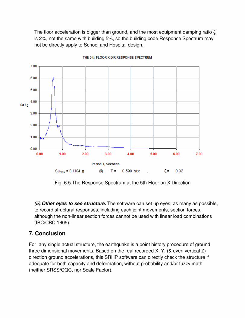
The floor acceleration is bigger than ground, and the most equipment damping ratio ζ

is 2%, not the same with building 5%, so the building code Response Spectrum may

not be directly apply to School and Hospital design.

Fig. 6.5 The Response Spectrum at the 5th Floor on X Direction

(5).Other eyes to see structure. The software can set up eyes, as many as possible,

to record structural responses, including each joint movements, section forces,

although the non-linear section forces cannot be used with linear load combinations

(IBC/CBC 1605).

7. Conclusion

For any single actual structure, the earthquake is a point history procedure of ground

three dimensional movements. Based on the real recorded X, Y, (& even vertical Z)

direction ground accelerations, this SRHP software can directly check the structure if

adequate for both capacity and deformation, without probability and/or fuzzy math

(neither SRSS/CQC, nor Scale Factor).

Reference

Li, Tian (1997). “A Study on Damping Values Applied to The Time-History Dynamic

Analysis of Structures,” China Civil Engineering Journal, 30 (3), 68-73.

Li, Tian, and Wu, Xuemin (1992). “Elasto-Plastic Dynamic Analysis of Multistory and

Complex Structures at Multi-Dimensional Ground Accelerations,” Journal of Building

Structures, P. R. China, 13 (6), 2-11.

CBC (2010). California Building Code, California Building Standards Commission,

Sacramento, CA.

IBC (2009). International Building Code, International Code Council, Washington, DC.

ASCE 7 (2010). Minimum Design Loads for Buildings and Other Structures (ASCE/SEI

7-10), American Society of Civil Engineers, Reston, VA.

ACI 318 (2008). Building Code Requirements for Structural Concrete (ACI 318-08) and

Commentary, American Concrete Institute, Farmington Hills, MI.

AISC 360 (2005). Specification for Structural Steel Buildings (AISC 360-05), American

Institute of Steel Construction, Chicago, IL.

AISC 341 (2005). Seismic Provisions for Structural Steel Buildings (AISC 341-05),

American Institute of Steel Construction, Chicago, IL.

AISC 358 (2009). Prequalified Connections for Special and Intermediate Steel Moment

Frames for Seismic Applications (ANSI/AISC 358-05s1-09), American Institute of Steel

Construction, Chicago, IL.

ASCE 41 (2007). Seismic Rehabilitation of Existing Buildings (ASCE/SEI 41-06),

American Society of Civil Engineers, Reston, VA.

Abbreviations

2D: Two Dimensional

3D: Three Dimensional

DOF: Degree of Freedom

Gravity-BM: Gravity Beam

Gravity-COL: Gravity Column

SMF-BM: Beam of Special Moment

Frame

SMF-COL: Column of Special

Moment Frame

SRSS: Square Root of Sum of

Squares

Q & AQ & AQ & AQ & A

1. Why this SRHP software results have made a big difference with others?

The SRHP software is more accurate than Modal Superposition Method, because the

Modal Superposition Method is a probability method, which always requires a Scale

Factor (ASCE 7 12.9.2, 12.9.4, & CBC 1614A.1.9) with SRSS/CQC, or even just SUM,

to reach the determined analysis results.

2. Why the structural periods have to be calculated at each time step?

The physical damping concept is a passive force/load, not constant one. When

structural stiffness (periods) changed, the damping matrix [c] has to be updated, at each

time step.

3. Why the SRHP software does not include nonlinear shear wall?

The software can input nonlinear shear wall, since opening system. But as lateral frame,

shear wall cannot be designed with plastic hinges. Based on ACI 318-08 Chapter 21,

the SD level elastic section forces are always used to check shear wall capacity if

adequate, which means that the shear wall is linear within φMn capacity. Out-of fMn

capacity, the shear wall, no matter its linear or nonlinear, cannot be as lateral frame any

more.

Shear wall may keep gravity capacity, at upper-bound seismic load, but not plastic

hinge stiffness (dog bone).

4. Why the SRHP used 2D frame, not directly 3D?

The most lateral resisting frames are built by W-Shape steel with almost zero torsional

stiffness, and/or by concrete element with brittle torsional crushing. The current 3D

element stiffness matrix (12 x 12) cannot cover them well.

Although ASCE 7-10 included 3D nonlinear section, the upper level 2010 CBC general

section 1.1.7 say that the specific provision shall apply in the event of any differences

between ASCE 7 and ACI/AISC, so the 2D frame, based on ACI 318-08 Chapter 21 and

AISC 341-05/AISC 358-05, still governs lateral design.

5. Why the SRHP does not calculate LL, Wind, & P∆∆∆∆?

Before the load combinations (IBC/CBC 1605), all loads have to be known. Also, all

load combinations are linear point combinations, not nonlinear history procedure

combinations.

This SRHP software is focus on getting correct seismic load (equivalent base shear

force) and the maximum ∆∆∆∆ value.

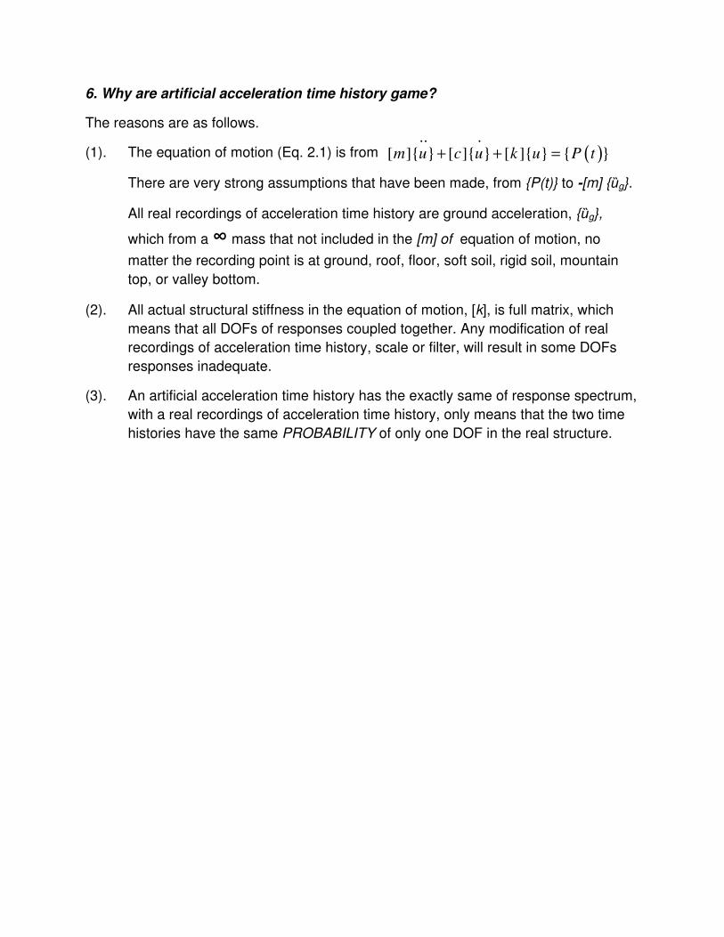
6. Why are artificial acceleration time history game?

The reasons are as follows.

(1). The equation of motion (Eq. 2.1) is from

There are very strong assumptions that have been made, from P(t) to -[m] ȕg.

All real recordings of acceleration time history are ground acceleration, ȕg,

which from a ∞ mass that not included in the [m] of equation of motion, no

matter the recording point is at ground, roof, floor, soft soil, rigid soil, mountain

top, or valley bottom.

(2). All actual structural stiffness in the equation of motion, [k], is full matrix, which

means that all DOFs of responses coupled together. Any modification of real

recordings of acceleration time history, scale or filter, will result in some DOFs

responses inadequate.

(3). An artificial acceleration time history has the exactly same of response spectrum,

with a real recordings of acceleration time history, only means that the two time

histories have the same PROBABILITY of only one DOF in the real structure.

( ).. .

[ ] [ ] [ ] m u c u k u P t+ + =