nonlinear regression analysis and its applications · applications. nonlinear regression ......
TRANSCRIPT

Nonlinear Regression Analysis and Its
Applications


Nonlinear RegressionAnalysis and Its Applications
Second edition
Douglas M. Bates and Donald G. Watts
A Wiley-Interscience Publication
JOHN WILEY & SONS, INC.
New York / Chichester / Weinheim / Brisbane / Singapore / Toronto


Preface
text...
This is a preface section
text...
v


Acknowledgments
To Mary Ellen and Valery
vii


Contents
Preface v
Acknowledgments vii
1 Review of Linear Regression 1
1.1 The Linear Regression Model 1
1.1.1 The Least Squares Estimates 4
1.1.2 Sampling Theory Inference Results 5
1.1.3 Likelihood Inference Results 7
1.1.4 Bayesian Inference Results 7
1.1.5 Comments 7
1.2 The Geometry of Linear Least Squares 9
1.2.1 The Expectation Surface 10
1.2.2 Determining the Least Squares Estimates 12
1.2.3 Parameter Inference Regions 15
1.2.4 Marginal Confidence Intervals 19
1.2.5 The Geometry of Likelihood Results 23
1.3 Assumptions and Model Assessment 24
1.3.1 Assumptions and Their Implications 25
1.3.2 Model Assessment 27
1.3.3 Plotting Residuals 28
ix

x CONTENTS
1.3.4 Stabilizing Variance 29
1.3.5 Lack of Fit 30
Problems 31
2 Nonlinear Regression 33
2.1 The Nonlinear Regression Model 33
2.1.1 Transformably Linear Models 35
2.1.2 Conditionally Linear Parameters 37
2.1.3 The Geometry of the Expectation Surface 37
2.2 Determining the Least Squares Estimates 40
2.2.1 The Gauss–Newton Method 2 2 1 41
2.2.2 The Geometry of Nonlinear Least Squares 43
2.2.3 Convergence 50
2.3 Nonlinear Regression Inference Using the LinearApproximation 53
2.3.1 Approximate Inference Regions forParameters 2 3 1 54
2.3.2 Approximate Inference Bands for theExpected Response 58
2.4 Nonlinear Least Squares via Sums of Squares 62
2.4.1 The Linear Approximation 62
2.4.2 Overshoot 67
Problems 67
Appendix A Data Sets Used in Examples 69
A.1 PCB 69
A.2 Rumford 70
A.3 Puromycin 70
A.4 BOD 71
A.5 Isomerization 73
A.6 α-Pinene 74
A.7 Sulfisoxazole 75
A.8 Lubricant 76
A.9 Chloride 76
A.10 Ethyl Acrylate 76
A.11 Saccharin 79
A.12 Nitrite Utilization 80
A.13 s-PMMA 82
A.14 Tetracycline 82

CONTENTS xi
A.15 Oil Shale 82
A.16 Lipoproteins 85
References 87

1Review of Linear
Regression
Non sunt multiplicanda entia praeter necessitatem.(Entities are not to be multiplied beyond necessity.)
—William of Ockham
We begin with a brief review of linear regression, because a thoroughgrounding in linear regression is fundamental to understanding nonlinear re-gression. For a more complete presentation of linear regression see, for ex-ample, Draper and Smith (1981), Montgomery and Peck (1982), or Seber(1977). Detailed discussion of regression diagnostics is given in Belsley, Kuhand Welsch (1980) and Cook and Weisberg (1982), and the Bayesian approachis discussed in Box and Tiao (1973).
Two topics which we emphasize are modern numerical methods and thegeometry of linear least squares. As will be seen, attention to efficient com-puting methods increases understanding of linear regression, while the geo-metric approach provides insight into the methods of linear least squares andthe analysis of variance, and subsequently into nonlinear regression.
1.1 THE LINEAR REGRESSION MODEL
Linear regression provides estimates and other inferential results for the pa-
rameters β = (β1, β2, . . . , βP )T in the model
Yn = β1xn1 + β2xn2 + · · · + βP xnP + Zn (1.1)
= (xn1, . . . , xnP )β + Zn
1

2 REVIEW OF LINEAR REGRESSION
In this model, the random variable Yn, which represents the response forcase n, n = 1, 2, . . . , N , has a deterministic part and a stochastic part. Thedeterministic part, (xn1, . . . , xnP )β, depends upon the parameters β and uponthe predictor or regressor variables xnp, p = 1, 2, . . . , P . The stochastic part,represented by the random variable Zn, is a disturbance which perturbs theresponse for that case. The superscript T denotes the transpose of a matrix.
The model for N cases can be written
Y = Xβ + Z (1.2)
where Y is the vector of random variables representing the data we may get,X is the N × P matrix of regressor variables,
X =
x11
x21
.
.
.xN1
x12
x22
.
.
.xN2
x13
x23
.
.
.xN3
. . .
. . .
. . .
x1P
x2P
.
.
.xNP
and Z is the vector of random variables representing the disturbances. (Wewill use bold face italic letters for vectors of random variables.)
The deterministic part, Xβ, a function of the parameters and the regres-sor variables, gives the mathematical model or the model function for theresponses. Since a nonzero mean for Zn can be incorporated into the modelfunction, we assume that
E[Z] = 0 (1.3)
or, equivalently,E[Y ] = Xβ
We therefore call Xβ the expectation function for the regression model. Thematrix X is called the derivative matrix , since the (n, p)th term is the deriva-tive of the nth row of the expectation function with respect to the pth pa-rameter.
Note that for linear models, derivatives with respect to any of the parame-
ters are independent of all the parameters.If we further assume that Z is normally distributed with
Var[Z] = E[ZZT] = σ2I (1.4)
where I is an N×N identity matrix, then the joint probability density functionfor Y , given β and the variance σ2, is
p(y|β, σ2) =(
2πσ2)
−N/2exp
(
− (y − Xβ)T
(y − Xβ)
2σ2
)
(1.5)
=(
2πσ2)
−N/2exp
(−‖y − Xβ‖2
2σ2
)

THE LINEAR REGRESSION MODEL 3
••••
••• ••
•
••• •
•
••
••
•
•
•
•
•
••
•
•
Age (years)
PC
B c
once
ntra
tion
(ppm
)
2 4 6 8 10 12
05
1015
2025
30
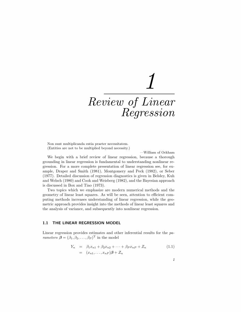
Fig. 1.1 Plot of PCB concentration versus age for lake trout.
where the double vertical bars denote the length of a vector. When providedwith a derivative matrix X and a vector of observed data y, we wish to makeinferences about σ2 and the P parameters β.Example:
As a simple example of a linear regression model, we consider the con-centration of polychlorinated biphenyls (PCBs) in Lake Cayuga trout asa function of age (Bache, Serum, Youngs and Lisk, 1972). The data setis described in Appendix 1, Section A1.1. A plot of the PCB concentra-tion versus age, Figure 1.1, reveals a curved relationship between PCBconcentration and age. Furthermore, there is increasing variance in thePCB concentration as the concentration increases. Since the assump-tion (1.4) requires that the variance of the disturbances be constant,we seek a transformation of the PCB concentration which will stabilizethe variance (see Section 1.3.2). Plotting the PCB concentration on alogarithmic scale, as in Figure 1.2a, nicely stabilizes the variance andproduces a more nearly linear relationship. Thus, a linear expectationfunction of the form
ln(PCB) = β1 + β2 age
could be considered appropriate, where ln denotes the natural logarithm(logarithm to the base e). Transforming the regressor variable (Box andTidwell, 1962) can produce an even straighter plot, as shown in Figure1.2b, where we use the cube root of age. Thus a simple expectation

4 REVIEW OF LINEAR REGRESSION
•
•
•
•
•
•
• ••
•
••• •
•
••
••
•
••
•
•
• •
•
•
Age (years)
PC
B c
once
ntra
tion
(ppm
)
2 4 6 8 10 12
0.5
15
10
(a)
•
•
•
•
•
•
• ••
•
••• •
•
••
••
•
••
•
•
• •
•
•
Cube root of age
PC
B c
once
ntra
tion
(ppm
)
1.0 1.2 1.4 1.6 1.8 2.0 2.2
0.5
15
10
(b)
Fig. 1.2 Plot of PCB concentration versus age for lake trout. The concentration, ona logarithmic scale, is plotted versus age in part a and versus 3
√age in part b.
function to be fitted is
ln(PCB) = β1 + β23√
age
(Note that the methods of Chapter 2 can be used to fit models of theform
f(x, β, α) = β0 + β1xα1
1 + β2xα2
2 + · · · + βP xαP
P
by simultaneously estimating the conditionally linear parameters β andthe transformation parameters α. The powers α1, . . . , αP are used totransform the factors so that a simple linear model in xα1
1 , . . . , xαP
P isappropriate. In this book we use the power α = 0.33 for the age variableeven though, for the PCB data, the optimal value is 0.20.) •
1.1.1 The Least Squares Estimates
The likelihood function, or more simply, the likelihood, l(β, σ|y), for β and σis identical in form to the joint probability density (1.5) except that l(β, σ|y)is regarded as a function of the parameters conditional on the observed data,rather than as a function of the responses conditional on the values of theparameters. Suppressing the constant (2π)−N/2 we write
l(β, σ|y) ∝ σ−N exp
(−‖y − Xβ‖2
2σ2
)
(1.6)
The likelihood is maximized with respect to β when the residual sum of
squares
S(β) = ‖y − Xβ‖2 (1.7)
THE LINEAR REGRESSION MODEL 5
=
N∑
n=1
[
yn −(
P∑
p=1
xnpβp
)]2
is a minimum. Thus the maximum likelihood estimate β is the value of β
which minimizes S(β). This β is called the least squares estimate and can bewritten
β = (XTX)−1XTy (1.8)
Least squares estimates can also be derived by using sampling theory, sincethe least squares estimator is the minimum variance unbiased estimator forβ, or by using a Bayesian approach with a noninformative prior density onβ and σ. In the Bayesian approach, β is the mode of the marginal posteriordensity function for β.
All three of these methods of inference, the likelihood approach, the sam-pling theory approach, and the Bayesian approach, produce the same pointestimates for β. As we will see shortly, they also produce similar regions of“reasonable” parameter values. First, however, it is important to realize thatthe least squares estimates are only appropriate when the model (1.2) and theassumptions on the disturbance term, (1.3) and (1.4), are valid. Expressed inanother way, in using the least squares estimates we assume:
1. The expectation function is correct.
2. The response is expectation function plus disturbance.
3. The disturbance is independent of the expectation function.
4. Each disturbance has a normal distribution.
5. Each disturbance has zero mean.
6. The disturbances have equal variances.
7. The disturbances are independently distributed.
When these assumptions appear reasonable and have been checked usingdiagnostic plots such as those described in Section 1.3.2, we can go on to makefurther inferences about the regression model.
Looking in detail at each of the three methods of statistical inference, wecan characterize some of the properties of the least squares estimates.
1.1.2 Sampling Theory Inference Results
The least squares estimator has a number of desirable properties as shown,for example, in Seber (1977):
1. The least squares estimator β is normally distributed. This followsbecause the estimator is a linear function of Y , which in turn is a linear

6 REVIEW OF LINEAR REGRESSION
function of Z. Since Z is assumed to be normally distributed, β isnormally distributed.
2. E[β] = β: the least squares estimator is unbiased.
3. Var[β] = σ2(XTX)−1: the covariance matrix of the least squares esti-mator depends on the variance of the disturbances and on the derivativematrix X.
4. A 1 − α joint confidence region for β is the ellipsoid
(β − β)TXTX(β − β) ≤ Ps2F (P, N − P ; α) (1.9)
where
s2 =S(β)
N − P
is the residual mean square or variance estimate based on N−P degrees
of freedom, and F (P, N − P ; α) is the upper α quantile for Fisher’s Fdistribution with P and N − P degrees of freedom.
5. A 1 − α marginal confidence interval for the parameter βp is
βp ± se(βp)t(N − P ; α/2) (1.10)
where t(N − P ; α/2) is the upper α/2 quantile for Student’s T distri-bution with N − P degrees of freedom and the standard error of theparameter estimator is
se(βp) = s
√
{
(XTX)−1}
pp(1.11)
with{
(XTX)−1}
ppequal to the pth diagonal term of the matrix (XTX)−1.
6. A 1 − α confidence interval for the expected response at x0 is
xT0 β ± s
√
xT0 (XTX)−1x0 t(N − P ; α/2) (1.12)
7. A 1 − α confidence interval for the expected response at x0 is
xT0 β ± s
√
xT0 (XTX)−1x0 t(N − P ; α/2) (1.13)
8. A 1 − α confidence band for the response function at any x is given by
xTβ ± s
√
xT(XTX)−1x√
PF (P, N − P ; α) (1.14)
The expressions (1.13) and (1.14) differ because (1.13) concerns an intervalat a single specific point, whereas (1.14) concerns the band produced by theintervals at all the values of x considered simultaneously.

THE LINEAR REGRESSION MODEL 7
1.1.3 Likelihood Inference Results
The likelihood l(β, σ | y), equation (1.6), depends on β only through ‖y −Xβ‖, so likelihood contours are of the form
‖y − Xβ‖2 = c (1.15)
where c is a constant. A likelihood region bounded by the contour for which
c = S(β)
[
1 +P
N − PF (P, N − P ; α)
]
is identical to a 1 − α joint confidence region from the sampling theory ap-proach. The interpretation of a likelihood region is quite different from thatof a confidence region, however.
1.1.4 Bayesian Inference Results
As shown in Box and Tiao (1973), the Bayesian marginal posterior densityfor β, assuming a noninformative prior density for β and σ of the form
p(β, σ) ∝ σ−1 (1.16)
is
p(β|y) ∝{
1 +(β − β)TXTX(β − β)
νs2
}
−(ν+P )/2
(1.17)
which is in the form of a P -variate Student’s T density with location pa-
rameter β, scaling matrix s2(XTX)−1, and ν = N − P degrees of freedom.Furthermore, the marginal posterior density for a single parameter βp, say, is
a univariate Student’s T density with location parameter βp, scale parameter
s2{
(XTX)−1}
pp, and degrees of freedom N − P . The marginal posterior
density for the mean of y at x0 is a univariate Student’s T density withlocation parameter xT
0 β, scale parameter s2xT0 (XTX)−1x0, and degrees of
freedom N − P .A highest posterior density (HPD) region of content 1 − α is defined (Box
and Tiao, 1973) as a region R in the parameter space such that Pr {β ∈ R} =1 − α and, for β1 ∈ R and β2 6∈ R, p(β1|y) ≥ p(β2|y). For linear modelswith a noninformative prior, an HPD region is therefore given by the ellipsoiddefined in (1.9). Similarly, the marginal HPD regions for βp and xT
0 β arenumerically identical to the sampling theory regions (1.11, 1.12, and 1.13).
1.1.5 Comments
Although the three approaches to statistical inference differ considerably, theylead to essentially identical inferences. In particular, since the joint confidence,
8 REVIEW OF LINEAR REGRESSION
likelihood, and Bayesian HPD regions are identical, we refer to them all asinference regions.
In addition, when referring to standard errors or correlations, we will usethe Bayesian term “the standard error of βp” when, for the sampling theoryor likelihood methods, we should more properly say “the standard error ofthe estimate of βp”.
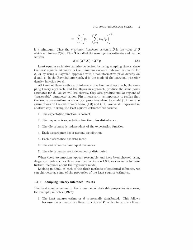
For linear least squares, any of the approaches can be used. For nonlinearleast squares, however, the likelihood approach has the simplest and mostdirect geometrical interpretation, and so we emphasize it.Example:
The PCB data can be used to determine parameter estimates and jointand marginal inference regions. In this linear situation, the regions canbe summarized using β, s2, XTX, and ν = N − P . For the ln(PCB)data with 3
√age as the regressor, we have β = (−2.391, 2.300)T , s2 =
0.246 on ν = 26 degrees of freedom, and
XT
X =
[
28.000 46.94146.941 83.367
]
(
XT
X
)
−1
=
[
0.6374 −0.3589−0.3589 0.2141
]
The joint 95% inference region is then
28.00(β1 + 2.391)2 + 93.88(β1 + 2.391)(β2 − 2.300) + 83.37(β2 − 2.300)2 = 2(0.246)3.37
= 1.66
the marginal 95% inference interval for the parameter β1 is
−2.391 ± (0.496)√
0.6374(2.056)
or−3.21 ≤ β1 ≤ −1.58
and the marginal 95% inference interval for the parameter β2 is
2.300 ± (0.496)√
0.2141(2.056)
or1.83 ≤ β2 ≤ 2.77
The 95% inference band for the ln(PCB) value at any 3√
age = x, is
−2.391 + 2.300x ± (0.496)√
0.637 − 0.718x + 0.214x2√
2(3.37)
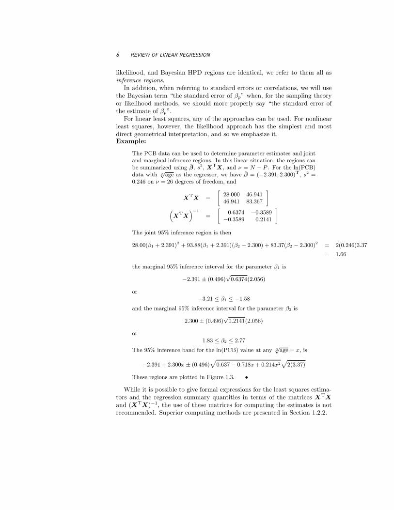
These regions are plotted in Figure 1.3. •
While it is possible to give formal expressions for the least squares estima-tors and the regression summary quantities in terms of the matrices XTX
and (XTX)−1, the use of these matrices for computing the estimates is notrecommended. Superior computing methods are presented in Section 1.2.2.
THE GEOMETRY OF LINEAR LEAST SQUARES 9
–3.5 –3.0 –2.5 –2.0 –1.5
1.8
2.0
2.2
2.4
2.6
2.8
+
β1
β 2
(a)
1.0 1.2 1.4 1.6 1.8 2.0 2.2
–10
12
3
Cube root of age
ln (
PC
B c
once
ntra
tion)
•
•
•
•
•
•
• ••
•
••• •
•
••
••
•
••
•
•
• •
•
•
(b)
Fig. 1.3 Inference regions for the model ln(PCB) = β1 + β2 3√
age. Part a shows theleast squares estimates (+), the parameter joint 95% inference region (solid line), andthe marginal 95% inference intervals (dotted lines). Part b shows the fitted response(solid line) and the 95% inference band (dotted lines).
Finally, the assumptions which lead to the use of the least squares estimatesshould always be examined when using a regression model. Further discussionon assumptions and their implications is given in Section 1.3.
1.2 THE GEOMETRY OF LINEAR LEAST SQUARES
The model (1.2) and assumptions (1.3) and (1.4) lead to the use of the leastsquares estimate (1.8) which minimizes the residual sum of squares (1.7). Asimplied by (1.7), S(β) can be regarded as the square of the distance from thedata vector y to the expected response vector Xβ. This links the subject oflinear regression to Euclidean geometry and linear algebra. The assumptionof a normally distributed disturbance term satisfying (1.3) and (1.4) indicatesthat the appropriate scale for measuring the distance between y and Xβ is theusual Euclidean distance between vectors. In this way the Euclidean geometryof the N -dimensional response space becomes statistically meaningful. Thisconnection between geometry and statistics is exemplified by the use of theterm spherical normal for the normal distribution with the assumptions (1.3)and (1.4), because then contours of constant probability are spheres.
Note that when we speak of the linear form of the expectation functionXβ, we are regarding it as a function of the parameters β, and that whendetermining parameter estimates we are only concerned with how the expectedresponse depends on the parameters, not with how it depends on the variables.In the PCB example we fit the response to 3
√age using linear least squares
because the parameters β enter the model linearly.
10 REVIEW OF LINEAR REGRESSION
1.2.1 The Expectation Surface
The process of calculating S(β) involves two steps:
1. Using the P -dimensional parameter vector β and the N × P derivativematrix X to obtain the N -dimensional expected response vector η(β) =Xβ, and
2. Calculating the squared distance from η(β) to the observed response y,‖y − η(β)‖2.
The possible expected response vectors η(β) form a P -dimensional expec-
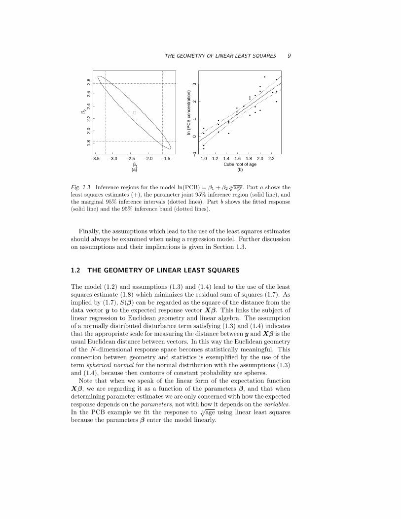
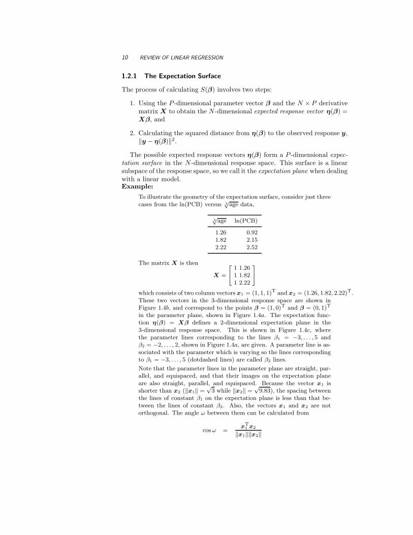
tation surface in the N -dimensional response space. This surface is a linearsubspace of the response space, so we call it the expectation plane when dealingwith a linear model.Example:
To illustrate the geometry of the expectation surface, consider just threecases from the ln(PCB) versus 3
√age data,
3√
age ln(PCB)
1.26 0.921.82 2.152.22 2.52
The matrix X is then
X =
[
111
1.261.822.22
]
which consists of two column vectors x1 = (1, 1, 1)T and x2 = (1.26, 1.82, 2.22)T.These two vectors in the 3-dimensional response space are shown inFigure 1.4b, and correspond to the points β = (1, 0)T and β = (0, 1)T
in the parameter plane, shown in Figure 1.4a. The expectation func-tion η(β) = Xβ defines a 2-dimensional expectation plane in the3-dimensional response space. This is shown in Figure 1.4c, wherethe parameter lines corresponding to the lines β1 = −3, . . . , 5 andβ2 = −2, . . . , 2, shown in Figure 1.4a, are given. A parameter line is as-sociated with the parameter which is varying so the lines correspondingto β1 = −3, . . . , 5 (dotdashed lines) are called β2 lines.
Note that the parameter lines in the parameter plane are straight, par-allel, and equispaced, and that their images on the expectation planeare also straight, parallel, and equispaced. Because the vector x1 isshorter than x2 (‖x1‖ =
√3 while ‖x2‖ =
√9.83), the spacing between
the lines of constant β1 on the expectation plane is less than that be-tween the lines of constant β2. Also, the vectors x1 and x2 are notorthogonal. The angle ω between them can be calculated from
cos ω =xT
1 x2
‖x1‖‖x2‖

THE GEOMETRY OF LINEAR LEAST SQUARES 11
β1
β 2
–2 0 2 4
–2–1
01
2
•
•
(0,1)T
(1,0)T
(a)
•
• (1,1,1)T
(1.26,1.82,2.22)T
1
2
η1
1
2
η3
1
2η2
(b)
1
2
η1
1
2
η2
β1 = 0
β1 = 2 β2 = 0
β2 = –1
β2 = –2
(c)
Fig. 1.4 Expectation surface for the 3-case PCB example. Part a shows the parameterplane with β1 parameter lines (dashed) and β2 parameter lines (dot–dashed). Part bshows the vectors x1 (dashed line) and x2 (dot–dashed line) in the response space.The end points of the vectors correspond to β = (1, 0)T and β = (0, 1)T respectively.Part c shows a portion of the expectation plane (shaded) in the response space, withβ1 parameter lines (dashed) and β2 parameter lines (dot–dashed).
12 REVIEW OF LINEAR REGRESSION
=5.30
√
(3)(9.83)
= 0.98
to be about 11◦, so the parameter lines on the expectation plane arenot at right angles as they are on the parameter plane.
As a consequence of the unequal length and nonorthogonality of thevectors, unit squares on the parameter plane map to parallelograms onthe expectation plane. The area of the parallelogram is
‖x1‖‖x2‖ sin ω = ‖x1‖‖x2‖√
1 − cos2 ω (1.18)
=
√
(xT1 x1)(xT
2 x2) − (xT1 x2)2
=
√
∣
∣XTX∣
∣
That is, the Jacobian determinant of the transformation from the pa-
rameter plane to the expectation plane is a constant equal to∣
∣XTX∣
∣
1/2.
Conversely, the ratio of areas in the parameter plane to those on the
expectation plane is∣
∣XTX∣
∣
−1/2. •
The simple linear mapping seen in the above example is true for all linearregression models. That is, for linear models, straight parallel equispacedlines in the parameter space map to straight parallel equispaced lines on theexpectation plane in the response space. Consequently, rectangles in one planemap to parallelepipeds in the other plane, and circles or spheres in one planemap to ellipses or ellipsoids in the other plane. Furthermore, the Jacobian
determinant,∣
∣
∣XTX
∣
∣
∣
1/2
, is a constant for linear models, and so regions of
fixed size in one plane map to regions of fixed size in the other, no matterwhere they are on the plane. These properties, which make linear least squaresespecially simple, are discussed further in Section 1.2.3.
1.2.2 Determining the Least Squares Estimates
The geometric representation of linear least squares allows us to formulate avery simple scheme for determining the parameters estimates β. Since theexpectation surface is linear, all we must do to determine the point on thesurface which is closest to the point y, is to project y onto the expectationplane. This gives us η, and β is then simply the value of β corresponding toη.
One approach to defining this projection is to observe that, after the projec-tion, the residual vector y−η will be orthogonal, or normal, to the expectationplane. Equivalently, the residual vector must be orthogonal to all the columnsof the X matrix, so
XT(y − Xβ) = 0

THE GEOMETRY OF LINEAR LEAST SQUARES 13
which is to say that the least squares estimate β satisfies the normal equations
XTXβ = XTy (1.19)
Because of (1.19) the least squares estimates are often written β = (XTX)−1XTy
as in (1.8). However, another way of expressing the estimate, and a more sta-ble way of computing it, involves decomposing X into the product of anorthogonal matrix and an easily inverted matrix. Two such decompositionsare the QR decomposition and the singular value decomposition (Dongarra,Bunch, Moler and Stewart, 1979, Chapters 9 and 11). We use the QR decom-position, where
X = QR
with the N × N matrix Q and the N × P matrix R constructed so that Q
is orthogonal (that is, QTQ = QQT = I) and R is zero below the maindiagonal. Writing
R =
[
R1
0
]
where R1 is P × P and upper triangular, and
Q = [Q1|Q2]
with Q1 the first P columns and Q2 the last N − P columns of Q, we have
X = QR = Q1R1 (1.20)
Performing a QR decomposition is straightforward, as is shown in Appendix2.
Geometrically, the columns of Q define an orthonormal, or orthogonal, basisfor the response space with the property that the first P columns span theexpectation plane. Projection onto the expectation plane is then very easy ifwe work in the coordinate system given by Q. For example we transform theresponse vector to
w = QTy (1.21)
with componentsw1 = QT
1 y (1.22)
andw2 = QT
2 y (1.23)
The projection of w onto the expectation plane is then simply[
w1
0
]
in the Q coordinates and
η = Q
[
w1
0
]
= Q1w1 (1.24)
14 REVIEW OF LINEAR REGRESSION
• y
1
2
η12
η2
•
•
•
q1
q3
q2
(a)
• w
1
2
q1
1
2
2
q2
w2
(b)
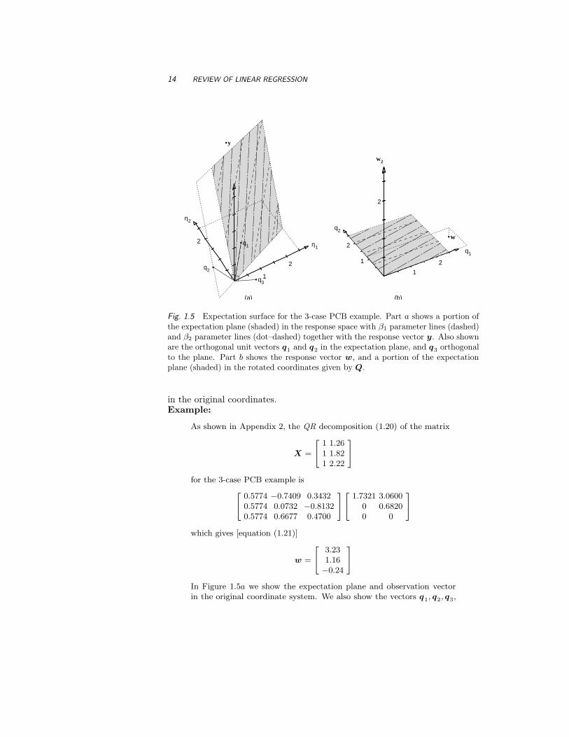
Fig. 1.5 Expectation surface for the 3-case PCB example. Part a shows a portion ofthe expectation plane (shaded) in the response space with β1 parameter lines (dashed)and β2 parameter lines (dot–dashed) together with the response vector y. Also shownare the orthogonal unit vectors q1 and q2 in the expectation plane, and q3 orthogonalto the plane. Part b shows the response vector w, and a portion of the expectationplane (shaded) in the rotated coordinates given by Q.
in the original coordinates.Example:
As shown in Appendix 2, the QR decomposition (1.20) of the matrix
X =
[
111
1.261.822.22
]
for the 3-case PCB example is
[
0.57740.57740.5774
−0.74090.07320.6677
0.3432−0.81320.4700
][
1.732100
3.06000.6820
0
]
which gives [equation (1.21)]
w =
[
3.231.16−0.24
]
In Figure 1.5a we show the expectation plane and observation vectorin the original coordinate system. We also show the vectors q1, q2, q3,
THE GEOMETRY OF LINEAR LEAST SQUARES 15
which are the columns of Q. It can be seen that q1 and q2 lie inthe expectation plane and q3 is orthogonal to it. In Figure 1.5b weshow, in the transformed coordinates, the observation vector and theexpectation plane, which is now horizontal. Note that projecting w
onto the expectation plane is especially simple, since it merely requiresreplacing the last element in w by zero. •
To determine the least squares estimate we must find the value β corre-sponding to η. Since
η = Xβ
using (1.24) and (1.20)
R1β = w1 (1.25)
and we solve for β by back-substitution (Stewart, 1973).Example:
For the complete ln(PCB), 3√
age data set,
R1 =[
5.291500
8.871052.16134
]
and w1 = (7.7570, 4.9721)T , so β = (−2.391, 2.300)T . •
1.2.3 Parameter Inference Regions
Just as the least squares estimates have informative geometric interpretations,so do the parameter inference regions (1.9), (1.10), (1.15) and those derivedfrom (1.17). Such interpretations are helpful for understanding linear regres-sion, and are essential for understanding nonlinear regression. (The geometricinterpretation is less helpful in the Bayesian approach, so we discuss only thesampling theory and likelihood approaches.)
The main difference between the likelihood and sampling theory geometricinterpretations is that the likelihood approach centers on the point y and thelength of the residual vector at η(β) compared to the shortest residual vector,while the sampling theory approach focuses on possible values of η(β) andthe angle that the resulting residual vectors could make with the expectationplane.
1.2.3.1 The Geometry of Sampling Theory Results To develop the geomet-ric basis of linear regression results from the sampling theory approach, wetransform to the Q coordinate system. The model for the random variableW = QTY is
W = Rβ + QTZ
or
U = W − Rβ (1.26)
where U = QTZ.

16 REVIEW OF LINEAR REGRESSION
The spherical normal distribution of Z is not affected by the orthogonaltransformation, so U also has a spherical normal distribution. This can be es-tablished on the basis of the geometry, since the spherical probability contourswill not be changed by a rigid rotation or reflection, which is what an orthogo-nal transformation must be. Alternatively, this can be established analyticallybecause QTQ = I , so the determinant of Q is ±1 and ‖Qx‖ = ‖x‖ for any N -vector x. Now the joint density for the random variables Z = (Z1, . . . , Zn)T
is
pZ(z) = (2πσ2)−N/2 exp
(−zTz
2σ2
)
and, after transformation, the joint density for U = QTZ is
pU (u) = (2πσ2)−N/2|Q| exp
(
−uTQTQu
2σ2
)
= (2πσ2)−N/2 exp
(−uTu
2σ2
)
From (1.26), the form of R leads us to partition U into two components:
U =
[
U 1
U 2
]
where U 1 consists of the first P elements of U , and U 2 the remaining N −Pelements. Each of these components has a spherical normal distribution ofthe appropriate dimension. Furthermore, independence of elements in theoriginal disturbance vector Z leads to independence of the elements of U , sothe components U 1 and U 2 are independent.
The dimensions νi of the components U i, called the degrees of freedom,are ν1 = P and ν2 = N − P . The sum of squares of the coordinates of aν-dimensional spherical normal vector has a σ2χ2 distribution on ν degrees offreedom, so
‖U1‖2 ∼ σ2χ2P
‖U2‖2 ∼ σ2χ2N−P
where the symbol ∼ is read “is distributed as.” Using the independence ofU 1 and U 2, we have
‖U1‖2/P
‖U2‖2/(N − P )∼ F (P, N − P ) (1.27)
since the scaled ratio of two independent χ2 random variables is distributedas Fisher’s F distribution.
The distribution (1.27) gives a reference distribution for the ratio of thesquared component lengths or, equivalently, for the angle that the disturbance

THE GEOMETRY OF LINEAR LEAST SQUARES 17
vector makes with the horizontal plane. We may therefore use (1.26) and(1.27) to test the hypothesis that β equals some specific value, say β0, bycalculating the residual vector u0 = QTy − Rβ0 and comparing the lengthsof the components u0
1 and u02 as in (1.27). The reasoning here is that a large
‖u01‖ compared to ‖u0
2‖ suggests that the vector y is not very likely to havebeen generated by the model (1.2) with β = β0, since u0 has a suspiciouslylarge component in the Q1 plane.
Note that‖u0
2‖2
N − P=
S(β)
N − P= s2
and‖u0
1‖2 = ‖R1β0 − w1‖2 (1.28)
and so the ratio (1.27) becomes
‖R1β0 − w1‖2
Ps2(1.29)
Example:
We illustrate the decomposition of the residual u for testing the nullhypothesis
H0 : β = (−2.0, 2.0)T
versus the alternative
HA : β 6= (−2.0, 2.0)T
for the full PCB data set in Figure 1.6. Even though the rotateddata vector w and the expectation surface for this example are in a28-dimensional space, the relevant distances can be pictured in the 3-dimensional space spanned by the expectation surface (vectors q1 andq2) and the residual vector. The scaled lengths of the components u1
and u2 are compared to determine if the point β0 = (−2.0, 2.0)T isreasonable.
The numerator in (1.29) is
∥
∥
∥
[
5.291500
8.871052.16134
] [ −2.02.0
]
−[
7.75704.9721
]∥
∥
∥
2
= 0.882
The ratio is then 0.882/(2 × 0.246) = 1.79, which corresponds to a tailprobability (or p value) of 0.19 for an F distribution with 2 and 26degrees of freedom. Since the probability of obtaining a ratio at leastas large as 1.79 is 19%, we do not reject the null hypothesis. •
A 1 − α joint confidence region for the parameters β consists of all thosevalues for which the above hypothesis test is not rejected at level α. Thus, avalue β0 is within a 1 − α confidence region if
‖u01‖2/P
‖u02‖2/(N − P )
≤ F (P, N − P ; α)

18 REVIEW OF LINEAR REGRESSION
•
•
w
u0
u20
u10
R1 β0
78
910
q1
4
5
6
7
2
3
4
w2
q2
β2 = 2
β2 = 3
β1 = –2
β1 = –1
Fig. 1.6 A geometric interpretation of the test H0 : β = (−2.0, 2.0)T for the fullPCB data set. We show the projections of the response vector w and a portion of theexpectation plane projected into the 3-dimensional space given by the tangent vectorsq1 and q2, and the orthogonal component of the response vector, w2. For the testpoint β0, the residual vector u0 is decomposed into a tangential component u0
1 andan orthogonal component u0
2.

THE GEOMETRY OF LINEAR LEAST SQUARES 19
Since s2 does not depend on β0, the points inside the confidence region forma disk on the expectation plane defined by
‖u1‖2 ≤ Ps2F (P, N − P ; α)
Furthermore, from (1.25) and (1.28) we have
‖u1‖2 = ‖R1(β − β)‖2
so a point on the boundary of the confidence region in the parameter spacesatisfies
R1(β − β) =√
Ps2F (P, N − P ; α) d
where ‖d‖ = 1. That is, the confidence region is given by
{
β = β +√
Ps2F (P, N − P ; α)R−11 d | ‖d‖ = 1
}
(1.30)
Thus the region of “reasonable” parameter values is a disk centered at R1β onthe expectation plane and is an ellipse centered at β in the parameter space.Example:
For the ln(PCB) versus 3√
age data, β = (−2.391, 2.300)T and s2 =0.246 based on 26 degrees of freedom, so the 95% confidence disk onthe transformed expectation surface is
R1β =[
7.75704.9721
]
+ 1.288[
cos ωsin ω
]
where 0 ≤ ω ≤ 2π. The disk is shown in the expectation plane in Figure1.7a, and the corresponding ellipse
β =[ −2.391
2.300
]
+ 1.288[
0.188980
−0.775660.46268
] [
cos ωsin ω
]
is shown in the parameter plane in Figure 1.7b. •
1.2.4 Marginal Confidence Intervals
We can create a marginal confidence interval for a single parameter, say β1,by “inverting” a hypothesis test of the form
H0 : β1 = β01
versusHA : β1 6= β0
1
Any β01 for which H0 is not rejected at level α is included in the 1−α confidence
interval. To perform the hypothesis test, we choose any parameter vector with
β1 = β01 , say
(
β01 ,0T
)T, calculate the transformed residual vector u0, and
divide it into three components: the first component u01 of dimension P − 1

20 REVIEW OF LINEAR REGRESSION
• w•
7 8 9 10q14
56
7
2
3
4
q2
–3.5 –3.0 –2.5 –2.0 –1.5
1.8
2.0
2.2
2.4
2.6
2.8
+
β1
β 2
Fig. 1.7 The 95% confidence disk and parameter confidence region for the PCB data.Part a shows the response vector w and a portion of the expectation plane projectedinto the 3-dimensional space given by the tangent vectors q1 and q2, and the orthogonalcomponent of the response vector, w2. The 95% confidence disk (shaded) in theexpectation plane (part a) maps to the elliptical confidence region (shaded) in theparameter plane (part b).
and parallel to the hyperplane defined by β1 = β01 ; the second component
u02 of dimension 1 and in the expectation plane but orthogonal to the β0
1
hyperplane; and the third component u03 of length (N −P )s2 and orthogonal
to the expectation plane. The component u02 is the same for any parameter
β with β1 = β01 , and, assuming that the true β1 is β0
1 , the scaled ratio of thecorresponding random variables U2 and U 3 has the distribution
U22 /1
‖U3‖2/(N − P )∼ F (1, N − P )
Thus we reject H0 at level α if(
u02
)2s2F (1, N − P ; α)
Example:
To test the null hypothesis
H0 : β1 = −2.0
versus the alternativeHA : β1 6= −2.0
for the complete PCB data set, we decompose the transformed residualvector at β0 = (−2.0, 2.2)T into three components as shown in Figure1.8 and calculate the ratio
(
u02
)2
s2=
0.240
0.246
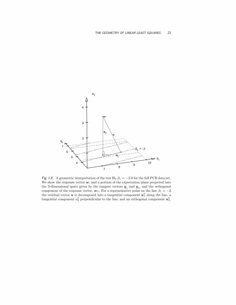
THE GEOMETRY OF LINEAR LEAST SQUARES 21
•
•
u
w
u3
u1u2
78
910
q1
4
5
6
7
2
3
4
q2
w2
β1 = –2
Fig. 1.8 A geometric interpretation of the test H0:β1 = −2.0 for the full PCB data set.We show the response vector w, and a portion of the expectation plane projected intothe 3-dimensional space given by the tangent vectors q1 and q2, and the orthogonalcomponent of the response vector, w2. For a representative point on the line β1 = −2the residual vector u is decomposed into a tangential component u0
1 along the line, atangential component u0
2 perpendicular to the line, and an orthogonal component u03.
22 REVIEW OF LINEAR REGRESSION
= 0.97
This corresponds to a p value of 0.33, and so we do not reject the nullhypothesis. •
We can create a 1 − α marginal confidence interval for β1 as all values forwhich
(
u02
)2 ≤ s2F (1, N − P ; α)
or, equivalently,|u0
2| ≤ s · t(N − P ; α/2) (1.31)
Since |u02| is the distance from the point R1β to the line corresponding to
β1 = β01 on the transformed parameter plane, the confidence interval will
include all values β01 for which the corresponding parameter line intersects
the disk{
R1β + st(N − P ; α/2)d | ‖d‖ = 1}
(1.32)
Instead of determining the value of |u02| for each β0
1 , we take the disk (1.32)and determine the minimum and maximum values of β1 for points on the disk.Writing r1 for the first row of R−1
1 , the values of β1 corresponding to pointson the expectation plane disk are
r1(R1β + s · t(N − P ; α/2)d) = β1 + s · t(N − P ; α/2)r1d
and the minimum and maximum occur for the unit vectors in the direction ofr1; that is, d = ±
(
r1)T
/‖r1‖. This gives the confidence interval
β1 ± s‖r1‖t(N − P ; α/2)
In general, a marginal confidence interval for parameter βp is
βp ± s‖rp‖t(N − P ; α/2) (1.33)
where rp is the pth row of R−11 . The quantity
se(βp) = s‖rp‖ (1.34)
is called the standard error for the pth parameter. Since
(XTX)−1 = (RT1 R1)
−1
= R−11 R−T
1
‖rp‖2 ={
(XTX)−1}
pp, so the standard error can be written as in equation
(1.11).A convenient summary of the variability of the parameter estimates can be
obtained by factoring R−11 as
R−11 = diag(‖r1‖, ‖r2‖, . . . , ‖rP ‖)L (1.35)

THE GEOMETRY OF LINEAR LEAST SQUARES 23
where L has unit length rows. The diagonal matrix provides the parameterstandard errors, while the correlation matrix
C = LLT (1.36)
gives the correlations between the parameter estimates.Example:
For the ln(PCB) data, β = (−2.391, 2.300)T, s2 = 0.246 with 26 degreesof freedom, and
R−11 =
[
5.291500
8.871052.16134
]
−1
=[
0.188980
−0.775660.46268
]
=[
0.7980
00.463
] [
0.2370
−0.9721
]
which gives standard errors of 0.798√
0.246 = 0.396 for β1 and 0.463√
0.246 =0.230 for β2. Also
C =[
1−0.972
−0.9721
]
so the correlation between β1 and β2 is −0.97. The 95% confidenceintervals for the parameters are given by −2.391 ± 2.056(0.396) and2.300 ± 2.056(0.230), which are plotted in Figure 1.3a. •
Marginal confidence intervals for the expected response at a design pointx0 can be created by determining which hyperplanes formed by constantxT
0 β intersect the disk (1.32). Using the same argument as was used toderive (1.33), we obtain a standard error for the expected response at x0 ass‖xT
0 R−11 ‖, so the confidence interval is
xT0 β ± s‖xT
0 R−11 ‖t(N − P ; α/2) (1.37)
Similarly, a confidence band for the response function is
xTβ ± s‖xTR−11 ‖√
PF (P, N − P ; α) (1.38)
Example:
A plot of the fitted expectation function and the 95% confidence bandsfor the PCB example was given in Figure 1.3b. •
Ansley (1985) gives derivations of other sampling theory results in linearregression using the QR decomposition, which, as we have seen, is closelyrelated to the geometric approach to regression.
1.2.5 The Geometry of Likelihood Results
The likelihood function indicates the plausibility of values of η relative to y,and consequently has a simple geometrical interpretation. If we allow η to
24 REVIEW OF LINEAR REGRESSION
take on any value in the N -dimensional response space, the likelihood contoursare spheres centered on y. Values of η of the form η = Xβ generate a P -dimensional expectation plane, and so the intersection of the plane with thelikelihood spheres produces disks.
Analytically, the likelihood function (1.6) depends on η through
‖η − y‖2 = ‖QT(η − y)‖2 (1.39)
= ‖QT1 (η − y)‖2 + ‖QT
2 (η − y)‖2
= ‖w(β) − w1‖2 + ‖w2‖2
where w(β) = QT1 η and QT
2 η = 0. A constant value of the total sum ofsquares specifies a disk of the form
‖w(β) − w1‖2 = c
on the expectation plane. Choosing
c = Ps2F (P, N − P ; α)
produces the disk corresponding to a 1−α confidence region. In terms of thetotal sum of squares, the contour is
S(β) = S(β)
{
1 +P
N − PF (P, N − P ; α)
}
(1.40)
As shown previously, and illustrated in Figure 1.7, this disk transforms toan ellipsoid in the parameter space.
1.3 ASSUMPTIONS AND MODEL ASSESSMENT
The statistical assumptions which lead to the use of the least squares esti-mates encompass several different aspects of the regression model. As withany statistical analysis, if the assumptions on the model and data are notappropriate, the results of the analysis will not be valid.
Since we cannot guarantee a priori that the different assumptions are allvalid, we must proceed in an iterative fashion as described, for example, inBox, Hunter and Hunter (1978). We entertain a plausible statistical model forthe data, analyze the data using that model, then go back and use diagnostics
such as plots of the residuals to assess the assumptions. If the diagnosticsindicate failure of assumptions in either the deterministic or stochastic com-ponents of the model, we must modify the model or the analysis and repeatthe cycle.
It is important to recognize that the design of the experiment and themethod of data collection can affect the chances of assumptions being validin a particular experiment. In particular randomization can be of great helpin ensuring the appropriateness of all the assumptions, and replication allowsgreater ability to check the appropriateness of specific assumptions.
ASSUMPTIONS AND MODEL ASSESSMENT 25
1.3.1 Assumptions and Their Implications
The assumptions, as listed in Section 1.1.1, are:
1. The expectation function is correct. Ensuring the validity of this as-sumption is, to some extent, the goal of all science. We wish to build amodel with which we can predict natural phenomena. It is in buildingthe mathematical model for the expectation function that we frequentlyfind ourselves in an iterative loop. We proceed as though the expecta-tion function were correct, but we should be prepared to modify it asthe data and the analyses dictate. In almost all linear, and in manynonlinear, regression situations we do not know the “true” model, butwe choose a plausible one by examining the situation, looking at dataplots and cross-correlations, and so on. As the analysis proceeds we canmodify the expectation function and the assumptions about the distur-bance term to obtain a more sensible and useful answer. Models shouldbe treated as just models, and it must be recognized that some will bemore appropriate or adequate than others. Nevertheless, assumption (1)is a strong one, since it implies that the expectation function includesall the important predictor variables in precisely the correct form, andthat it does not include any unimportant predictor variables. A usefultechnique to enable checking the adequacy of a model function is toinclude replications in the experiment. It is also important to actuallymanipulate the predictor variables and randomize the order in whichthe experiments are done, to ensure that causation, not correlation, isbeing determined (Box, 1960).
2. The response is expectation function plus disturbance. This assumptionis important theoretically, since it allows the probability density func-tion for the random variable Y describing the responses to be simplycalculated from the probability density function for the random variableZ describing the disturbances. Thus,
pY (y|β, σ2) = pZ(y − Xβ|σ2)
In practice, this assumption is closely tied to the assumption of constantvariance of the disturbances. It may be the case that the disturbancescan be considered as having constant variance, but as entering the modelmultiplicatively, since in many phenomena, as the level of the “signal”increases, the level of the “noise” increases. This lack of additivityof the disturbance will manifest itself as a nonconstant variance in thediagnostic plots. In both cases, the corrective action is the same—eitheruse weighted least squares or take a transformation of the response aswas done in Example PCB 1.
3. The disturbance is independent of the expectation function. This as-sumption is closely related to assumption (2), since they both relate to
26 REVIEW OF LINEAR REGRESSION
appropriateness of the additive model. One of the implications of thisassumption is that the control or predictor variables are measured per-fectly. Also, as a converse to the implication in assumption (1) that allimportant variables are included in the model, this assumption impliesthat any important variables which are not included are not systemat-
ically related to the response. An important technique to improve thechances that this is true is to randomize the order in which the ex-periments are done, as suggested by Fisher (1935). In this way, if animportant variable has been omitted, its effect may be manifested asa disturbance (and hence simply inflate the variability of the observa-tions) rather than being confounded with one of the predictor effects(and hence bias the parameter estimates). And, of course, it is impor-tant to actually manipulate the predictor variables not merely recordtheir values.
4. Each disturbance has a normal distribution. The assumption of normal-ity of the disturbances is important, since this dictates the form of thesampling distribution of the random variables describing the responses,and through this, the likelihood function for the parameters. This leadsto the criterion of least squares, which is enormously powerful becauseof its mathematical tractability. For example, given a linear model, it ispossible to write down the analytic solution for the parameter estima-tors and to show [Gauss’s theorem (Seber, 1977)] that the least squaresestimates are the best both individually and in any linear combination,in the sense that they have the smallest mean square error of any lin-ear estimators. The normality assumption can be justified by appealingto the central limit theorem, which states that the resultant of manydisturbances, no one of which is dominant, will tend to be normallydistributed. Since most experiments involve many operations to set upand measure the results, it is reasonable to assume, at least tentatively,that the disturbances will be normally distributed. Again, the assump-tion of normality will be more likely to be appropriate if the order ofthe experiments is randomized. The assumption of normality may bechecked by examining the residuals.
5. Each disturbance has zero mean. This assumption is primarily a sim-plifying one, which reduces the number of unknown parameters to amanageable level. Any nonzero mean common to all observations canbe accommodated by introducing a constant term in the expectationfunction, so this assumption is unimportant in linear regression. It canbe important in nonlinear regression, however, where many expectationfunctions occur which do not include a constant. The main implicationof this assumption is that there is no systematic bias in the disturbancessuch as could be caused by an unsuspected influential variable. Hence,we see again the value of randomization.
ASSUMPTIONS AND MODEL ASSESSMENT 27
6. The disturbances have equal variances. This assumption is more impor-tant practically than theoretically, since a solution exists for the leastsquares estimation problem for the case of unequal variances [see, e.g.,Draper and Smith (1981) concerning weighted least squares]. Practi-cally, however, one must describe how the variances vary, which canonly be done by making further assumptions, or by using informationfrom replications and incorporating this into the analysis through gener-alized least squares, or by transforming the data. When the variance isconstant, the likelihood function is especially simple, since the parame-ters can be estimated independently of the nuisance parameter σ2. Themain implication of this assumption is that all data values are equally
unreliable, and so the simple least squares criterion can be used. Theappropriateness of this assumption can sometimes be checked after amodel has been fitted by plotting the residuals versus the fitted values,but it is much better to have replications. With replications, we cancheck the assumption before even fitting a model, and can in fact usethe replication averages and variances to determine a suitable variance-
stabilizing transformation; see Section 1.3.2. Transforming to constantvariance often has the additional effect of making the disturbances be-have more normally. This is because a constant variance is necessarilyindependent of the mean (and anything else, for that matter), and thisindependence property is fundamental to the normal density.
7. The disturbances are distributed independently. The final assumptionis that the disturbances in different experiments are independent ofone another. This is an enormously simplifying assumption, becausethen the joint probability density function for the vector Y is just theproduct of the probability densities for the individual random variablesYn, n = 1, 2, . . . , N . The implication of this assumption is that the dis-turbances on separate runs are not systematically related, an assump-tion which can usually be made to be more appropriate by randomiza-tion. Nonindependent disturbances can be treated by generalized leastsquares, but, as in the case where there is nonconstant variance, modi-fications to the model must be made either through information gainedfrom the data, or by additional assumptions as to the nature of theinterdependence.
1.3.2 Model Assessment
In this subsection we present some simple methods for verifying the appropri-ateness of assumptions, especially through plots of residuals. Further discus-sion on regression diagnostics for linear models is given in Hocking (1983), andin the books by Belsley et al. (1980), Cook and Weisberg (1982), and Draperand Smith (1981). In Chapter 3 we discuss model assessment for nonlinearmodels.
28 REVIEW OF LINEAR REGRESSION
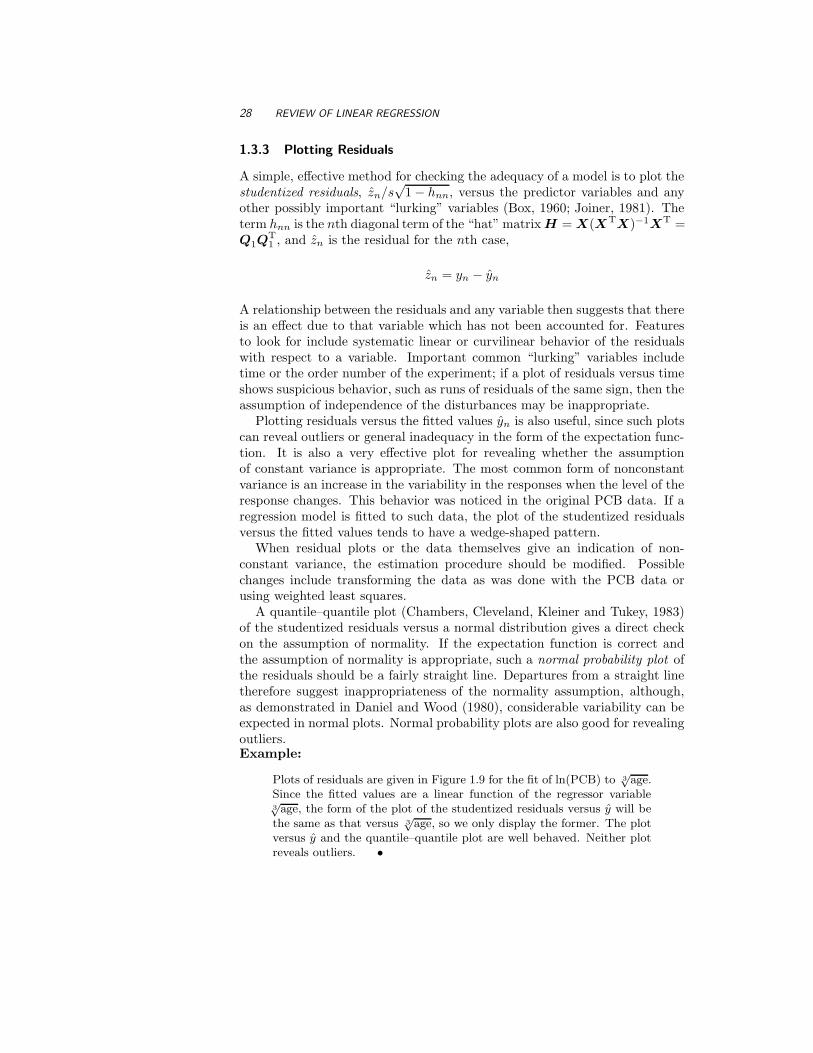
1.3.3 Plotting Residuals
A simple, effective method for checking the adequacy of a model is to plot thestudentized residuals, zn/s
√1 − hnn, versus the predictor variables and any
other possibly important “lurking” variables (Box, 1960; Joiner, 1981). Theterm hnn is the nth diagonal term of the “hat” matrix H = X(XTX)−1XT =Q1Q
T1 , and zn is the residual for the nth case,
zn = yn − yn
A relationship between the residuals and any variable then suggests that thereis an effect due to that variable which has not been accounted for. Featuresto look for include systematic linear or curvilinear behavior of the residualswith respect to a variable. Important common “lurking” variables includetime or the order number of the experiment; if a plot of residuals versus timeshows suspicious behavior, such as runs of residuals of the same sign, then theassumption of independence of the disturbances may be inappropriate.
Plotting residuals versus the fitted values yn is also useful, since such plotscan reveal outliers or general inadequacy in the form of the expectation func-tion. It is also a very effective plot for revealing whether the assumptionof constant variance is appropriate. The most common form of nonconstantvariance is an increase in the variability in the responses when the level of theresponse changes. This behavior was noticed in the original PCB data. If aregression model is fitted to such data, the plot of the studentized residualsversus the fitted values tends to have a wedge-shaped pattern.
When residual plots or the data themselves give an indication of non-constant variance, the estimation procedure should be modified. Possiblechanges include transforming the data as was done with the PCB data orusing weighted least squares.
A quantile–quantile plot (Chambers, Cleveland, Kleiner and Tukey, 1983)of the studentized residuals versus a normal distribution gives a direct checkon the assumption of normality. If the expectation function is correct andthe assumption of normality is appropriate, such a normal probability plot ofthe residuals should be a fairly straight line. Departures from a straight linetherefore suggest inappropriateness of the normality assumption, although,as demonstrated in Daniel and Wood (1980), considerable variability can beexpected in normal plots. Normal probability plots are also good for revealingoutliers.Example:
Plots of residuals are given in Figure 1.9 for the fit of ln(PCB) to 3√
age.Since the fitted values are a linear function of the regressor variable3√
age, the form of the plot of the studentized residuals versus y will bethe same as that versus 3
√age, so we only display the former. The plot
versus y and the quantile–quantile plot are well behaved. Neither plotreveals outliers. •
ASSUMPTIONS AND MODEL ASSESSMENT 29
•
•
•
••
•
•
••
•
••
••
•
••
•
•
•
•
•
•
•
••
•
•
Fitted values
Stu
dent
ized
res
idua
ls
0.0 0.5 1.0 1.5 2.0 2.5 3.0
–2–1
01
2
(a)
•• •
• • •••••
••••
•••••
••• • • •• •
•
Normal quantile
Stu
dent
ized
res
idua
ls
–2 –1 0 1 2
–2–1
01
2
(b)
Fig. 1.9 Studentized residuals for the PCB data plotted versus fitted values in parta and versus normal quantiles in part b.
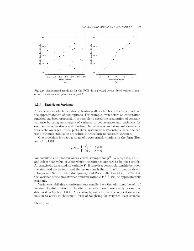
1.3.4 Stabilizing Variance
An experiment which includes replications allows further tests to be made onthe appropriateness of assumptions. For example, even before an expectationfunction has been proposed, it is possible to check the assumption of constantvariance by using an analysis of variance to get averages and variances foreach set of replications and plotting the variances and standard deviationsversus the averages. If the plots show systematic relationships, then one canuse a variance-stabilizing procedure to transform to constant variance.
One procedure is to try a range of power transformations in the form (Boxand Cox, 1964)
y(λ) =
{
yλ−1λ λ 6= 0
ln y λ = 0
We calculate and plot variances versus averages for y(λ), λ = 0,±0.5,±1, . . .and select that value of λ for which the variance appears to be most stable.Alternatively, for a random variable Y , if there is a power relationship betweenthe standard deviation σ and the mean µ such that σ ∝ µα, it can be shown(Draper and Smith, 1981; Montgomery and Peck, 1982; Box et al., 1978) thatthe variance of the transformed random variable Y 1−α will be approximatelyconstant.
Variance-stabilizing transformations usually have the additional benefit ofmaking the distribution of the disturbances appear more nearly normal, asdiscussed in Section 1.3.1. Alternatively, one can use the replication infor-mation to assist in choosing a form of weighting for weighted least squares.
Example:

30 REVIEW OF LINEAR REGRESSION
• •• •
••
•
•
Average (ppm)
Sta
ndar
d de
viat
ion
(ppm
)
0 5 10 15
02
46
810
(a)
•
••
•
•
•
•
•
Average (log scale)
Sta
ndar
d de
viat
ion
(log
scal
e)
0.0 0.5 1.0 1.5 2.0 2.5
0.2
0.3
0.4
0.5
0.6
0.7
(b)
Fig. 1.10 Replication standard deviations plotted versus replication averages for thePCB data in part a and for the ln(PCB) data in part b.
A plot of the standard deviations versus the averages for the originalPCB data is given in Figure 1.10a. It can be seen that there is agood straight line relationship between s and y, and so the variance-stabilizing technique leads to the logarithmic transformation. In Fig-ure 1.10b we plot the standard deviations versus the averages for theln(PCB) data. This plot shows no systematic relationship, and hencesubstantiates the effectiveness of the logarithmic transformation in sta-bilizing the variance. •
1.3.5 Lack of Fit
When the data set includes replications, it is also possible to perform tests forlack of fit of the expectation function. Such analyses are based on an analysisof variance in which the residual sum of squares S(β) with N − P degreesof freedom is decomposed into the replication sum of squares Sr (equal tothe total sum of squares of deviations of the replication values about theiraverages) with, say, νr degrees of freedom, and the lack of fit sum of squares
Sl = S(β)−Sr, with νl = fN −P − νr degrees of freedom. We then comparethe ratio of the lack of fit mean square over the replication mean square withthe appropriate value in the F table. That is, we compare
Sl/νl
Sr/νrwith F (νl, νr; α)
to determine whether there is significant lack of fit at level α. The geometricjustification for this analysis is that the replication subspace is always orthog-onal to the subspace containing the averages and the expectation function.
PROBLEMS 31
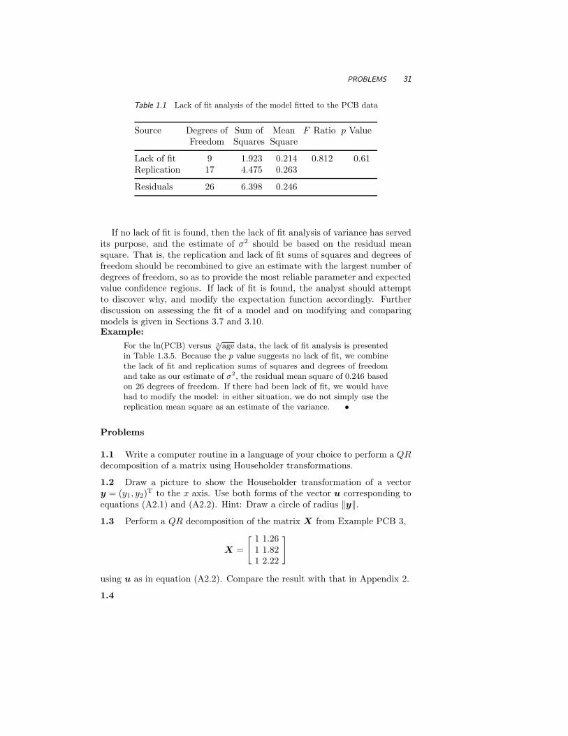
Table 1.1 Lack of fit analysis of the model fitted to the PCB data
Source Degrees of Sum of Mean F Ratio p ValueFreedom Squares Square
Lack of fit 9 1.923 0.214 0.812 0.61Replication 17 4.475 0.263
Residuals 26 6.398 0.246
If no lack of fit is found, then the lack of fit analysis of variance has servedits purpose, and the estimate of σ2 should be based on the residual meansquare. That is, the replication and lack of fit sums of squares and degrees offreedom should be recombined to give an estimate with the largest number ofdegrees of freedom, so as to provide the most reliable parameter and expectedvalue confidence regions. If lack of fit is found, the analyst should attemptto discover why, and modify the expectation function accordingly. Furtherdiscussion on assessing the fit of a model and on modifying and comparingmodels is given in Sections 3.7 and 3.10.Example:
For the ln(PCB) versus 3√
age data, the lack of fit analysis is presentedin Table 1.3.5. Because the p value suggests no lack of fit, we combinethe lack of fit and replication sums of squares and degrees of freedomand take as our estimate of σ2, the residual mean square of 0.246 basedon 26 degrees of freedom. If there had been lack of fit, we would havehad to modify the model: in either situation, we do not simply use thereplication mean square as an estimate of the variance. •
Problems
1.1 Write a computer routine in a language of your choice to perform a QRdecomposition of a matrix using Householder transformations.
1.2 Draw a picture to show the Householder transformation of a vectory = (y1, y2)
T to the x axis. Use both forms of the vector u corresponding toequations (A2.1) and (A2.2). Hint: Draw a circle of radius ‖y‖.1.3 Perform a QR decomposition of the matrix X from Example PCB 3,
X =
[
111
1.261.822.22
]
using u as in equation (A2.2). Compare the result with that in Appendix 2.
1.4

32 REVIEW OF LINEAR REGRESSION
1.4.1. Perform a QR decomposition of the matrix
D =
00010
11111
and obtain the matrix Q1. This matrix is used in Example α-pinene 6, Section4.3.4.
1.4.2. Calculate QT2 y, where y = (50.4, 32.9, 6.0, 1.5, 9.3)T, without ex-
plicitly solving for Q2.
1.5
1.5.1. Fit the model ln(PCB) = β1 + β2age to the PCB data and performa lack of fit analysis of the model. What do you conclude about the adequacyof this model?
1.5.2. Plot the residuals versus age, and assess the adequacy of the model.Now what do you conclude about the adequacy of the model?
1.5.3. Fit the model ln(PCB) = β1 +β2age+β3age2 to the PCB data andperform a lack of fit analysis of the model. What do you conclude about theadequacy of this model?
1.5.4. Perform an extra sum of squares analysis to determine whether thequadratic term is a useful addition.
1.5.5. Explain the difference between your answers in (a), (b), and (d).
2Nonlinear Regression:
Iterative Estimation andLinear Approximations
Although this may seem a paradox, all exact science is dominated by the idea ofapproximation.
—Bertrand Russell
Linear regression is a powerful method for analyzing data described bymodels which are linear in the parameters. Often, however, a researcher has amathematical expression which relates the response to the predictor variables,and these models are usually nonlinear in the parameters. In such cases,linear regression techniques must be extended, which introduces considerablecomplexity.
2.1 THE NONLINEAR REGRESSION MODEL
A nonlinear regression model can be written
Yn = f(xn, θ) + Zn (2.1)
where f is the expectation function and xn is a vector of associated regressorvariables or independent variables for the nth case. This model is of exactlythe same form as (1.1) except that the expected responses are nonlinear func-tions of the parameters. That is, for nonlinear models, at least one of the
derivatives of the expectation function with respect to the parameters depends
on at least one of the parameters.
33

34 NONLINEAR REGRESSION
To emphasize the distinction between linear and nonlinear models, we useθ for the parameters in a nonlinear model. As before, we use P for the numberof parameters.
When analyzing a particular set of data we consider the vectors xn, n =1, 2, . . . , N , as fixed and concentrate on the dependence of the expected re-sponses on θ. We create the N -vector η(θ) with nth element
ηn(θ) = f(xn, θ)n = 1, . . . , N
and write the nonlinear regression model as
Y = η(θ) + Z (2.2)
with Z assumed to have a spherical normal distribution. That is,
E[Z] = 0
Var(Z) = E[ZZT] = σ2I
as in the linear model.Example:
Count Rumford of Bavaria was one of the early experimenters on thephysics of heat. In 1798 he performed an experiment in which a cannonbarrel was heated by grinding it with a blunt bore. When the cannonhad reached a steady temperature of 130◦F, it was allowed to cooland temperature readings were taken at various times. The ambienttemperature during the experiment was 60◦F, so [under Newton’s lawof cooling, which states that df/dt = −θ(f−T0), where T0 is the ambienttemperature] the temperature at time t should be
f(t, θ) = 60 + 70e−θt
Since ∂f/∂θ = −70te−θt depends on the parameter θ, this model isnonlinear. Rumford’s data are presented in Appendix A, Section A.2.•
Example:
The Michaelis–Menten model for enzyme kinetics relates the initial“velocity” of an enzymatic reaction to the substrate concentration xthrough the equation
f(x, θ) =θ1x
θ2+x(2.3)
In Appendix A, Section A.3 we present data from Treloar (1974) onthe initial rate of a reaction for which the Michaelis–Menten modelis believed to be appropriate. The data, for an enzyme treated withPuromycin, are plotted in Figure 2.1.
Differentiating f with respect to θ1 and θ2 gives
∂f
∂θ1=
x
θ2 + x(2.4)
∂f
∂θ2=
−θ1x
(θ2 + x)2

THE NONLINEAR REGRESSION MODEL 35
•
•
••
•
•
••
••
••
Concentration (ppm)
Vel
ocity
((c
ount
s/m
in)/
min
)
0.0 0.2 0.4 0.6 0.8 1.0
050
100
150
200
Fig. 2.1 Plot of reaction velocity versus substrate concentration for the Puromycindata.
and since both these derivatives involve at least one of the parameters,the model is recognized as nonlinear. •
2.1.1 Transformably Linear Models
The Michaelis–Menten model (2.3) can be transformed to a linear model byexpressing the reciprocal of the velocity as a function of the reciprocal sub-strate concentration,
1
f=
1
θ1+
θ2
θ1
1
x(2.5)
= β1 + β2u
We call such models transformably linear. Some authors use the term “in-trinsically linear”, but we reserve the term “intrinsic” for a special geometricproperty of nonlinear models, as discussed in Chapter 7. As will be seen inChapter 3, transformably linear models have some advantages in nonlinearregression because it is easy to get starting values for some of the parameters.
It is important to understand, however, that a transformation of the datainvolves a transformation of the disturbance term too, which affects the as-sumptions on it. Thus, if we assume the model function (2.2) with an additive,spherical normal disturbance term is an appropriate representation of the ex-perimental situation, then these same assumptions will not be appropriate for
36 NONLINEAR REGRESSION
•
•
••
••
••••••
Concentration–1
Vel
ocity
–1
0 10 20 30 40 50
0.00
50.
010
0.01
50.
020
(a)Concentration
Vel
ocity
0.0 0.2 0.4 0.6 0.8 1.0 1.2
050
100
150
200
•
•
••
••
••
•• ••
(b)
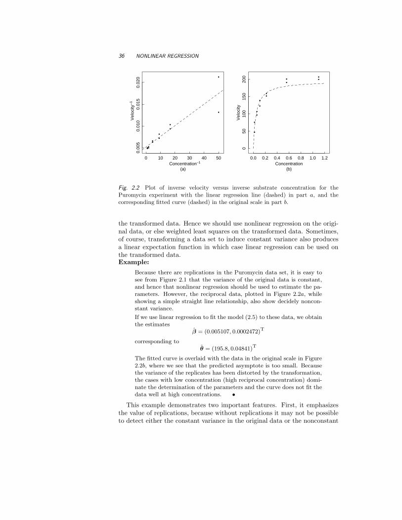
Fig. 2.2 Plot of inverse velocity versus inverse substrate concentration for thePuromycin experiment with the linear regression line (dashed) in part a, and thecorresponding fitted curve (dashed) in the original scale in part b.
the transformed data. Hence we should use nonlinear regression on the origi-nal data, or else weighted least squares on the transformed data. Sometimes,of course, transforming a data set to induce constant variance also producesa linear expectation function in which case linear regression can be used onthe transformed data.Example:
Because there are replications in the Puromycin data set, it is easy tosee from Figure 2.1 that the variance of the original data is constant,and hence that nonlinear regression should be used to estimate the pa-rameters. However, the reciprocal data, plotted in Figure 2.2a, whileshowing a simple straight line relationship, also show decidely noncon-stant variance.
If we use linear regression to fit the model (2.5) to these data, we obtainthe estimates
β = (0.005107, 0.0002472)T
corresponding toθ = (195.8, 0.04841)T
The fitted curve is overlaid with the data in the original scale in Figure2.2b, where we see that the predicted asymptote is too small. Becausethe variance of the replicates has been distorted by the transformation,the cases with low concentration (high reciprocal concentration) domi-nate the determination of the parameters and the curve does not fit thedata well at high concentrations. •
This example demonstrates two important features. First, it emphasizesthe value of replications, because without replications it may not be possibleto detect either the constant variance in the original data or the nonconstant

THE NONLINEAR REGRESSION MODEL 37
variance in the transformed data; and second, it shows that while transformingcan produce simple linear behavior, it also affects the disturbances.
2.1.2 Conditionally Linear Parameters
The Michaelis–Menten model is also an example of a model in which thereis a conditionally linear parameter, θ1. It is conditionally linear because thederivative of the expectation function with respect to θ1 does not involve θ1.We can therefore estimate θ1, conditional on θ2, by a linear regression ofvelocity x/(θ2 + x). Models with conditionally linear parameters enjoy someadvantageous properties, which can be exploited in nonlinear regression.
2.1.3 The Geometry of the Expectation Surface
The assumption of a spherical normal distribution for the disturbance termZ leads us to consider the Euclidean geometry of the N -dimensional responsespace, because again we will be interested in the least squares estimates θ ofthe parameters. The N -vectors η(θ) define a P -dimensional surface calledthe expectation surface in the response space, and the least squares estimatescorrespond to the point on the expectation surface,
η = η(θ)
which is closest to y. That is, θ minimizes the residual sum of squares
S(θ) = ‖y − η(θ)‖2
Example:
To illustrate the geometry of nonlinear models, consider the two casest = 4 and t = 41 for the Rumford data. Under the assumption thatNewton’s law of cooling holds for these data, the expected responsesare
η(θ) =[
60 + 70e−4θ
60 + 70e−41θ
]
θ ≥ 0
Substituting values for θ in these equations and plotting the pointsin a 2-dimensional response space gives the 1-dimensional expectationsurface (curve) shown in Figure 2.3.
Note that the expectation surface is curved and of finite extent , whichis in contrast to the linear model in which the expectation surface isa plane of infinite extent. Note, too, that points with equal spacingon the parameter line (θ) map to points with unequal spacing on theexpectation surface. •
Example:
As another example, consider the three cases from Example Puromycin2.1: x = 1.10, x = 0.56, and x = 0.22. Under the assumption that the

38 NONLINEAR REGRESSION
η1
η 2
0 20 40 60 80 100 120 140
020
4060
8010
012
014
0
∞
0
0.05
0.10.51
Fig. 2.3 Plot of the expectation surface (solid line) in the response space for the 2-caseRumford data. The points corresponding to θ = 0, 0.01, 0.02, . . . , 0.1, 0.2, . . . , 1,∞ aremarked.
expectation function (2.3) is the correct one, the expected responses forthese substrate values are
η(θ) =
θ1(1.10)θ2+1.10θ1(0.56)θ2+0.56θ1(0.22)θ2+0.22
θ1, θ2 ≥ 0
and so we can plot the expectation surface by substituting values for θ
in these equations. A portion of the 2-dimensional expectation surfacefor these x values is shown in Figure 2.4. Again, in contrast to the linearmodel, this expectation surface is not an infinite plane, and in general,straight lines in the parameter plane do not map to straight lines on theexpectation surface. It is also seen that unit squares in the parameterplane map to irregularly shaped areas on the expectation surface andthat the sizes of these areas vary. Thus, the Jacobian determinant isnot constant, which can be seen analytically, of course, because thederivatives (2.4) depend on θ.
For this model, there are straight lines on the expectation surface inFigure 2.4 corresponding to the θ1 parameter lines (lines with θ2 heldconstant), reflecting the fact that θ1 is conditionally linear. However,the θ1 parameter lines are neither parallel nor equispaced. The θ2 linesare not straight, parallel, or equispaced. •
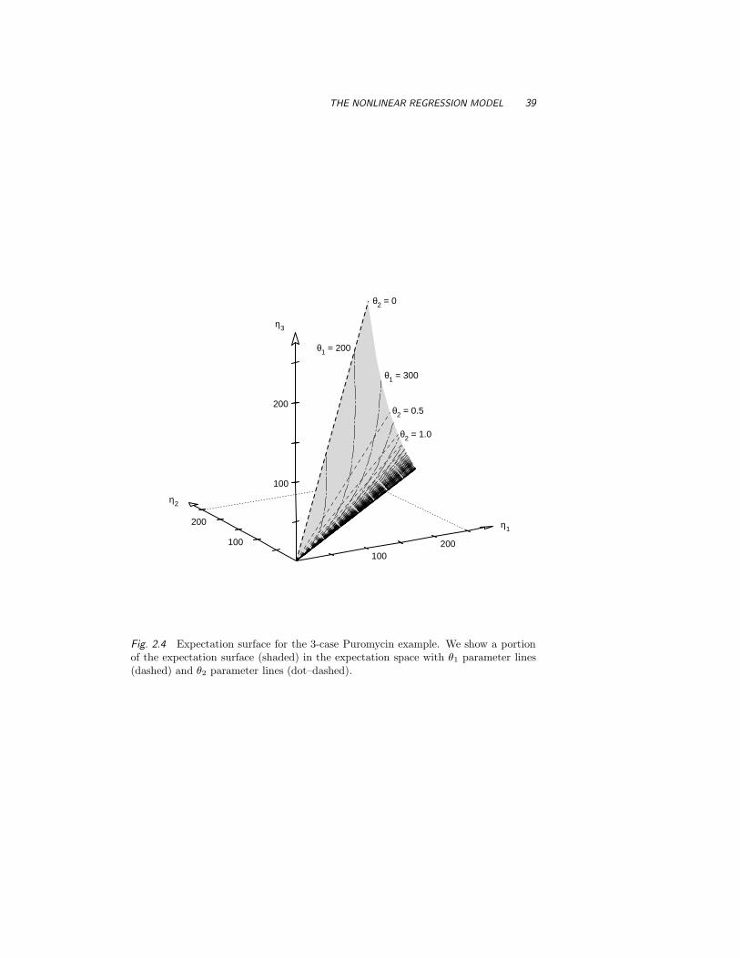
THE NONLINEAR REGRESSION MODEL 39
100200
η1
100
200
η3
100
200
η2
θ2 = 0
θ2 = 0.5
θ2 = 1.0
θ1 = 300
θ1 = 200
Fig. 2.4 Expectation surface for the 3-case Puromycin example. We show a portionof the expectation surface (shaded) in the expectation space with θ1 parameter lines(dashed) and θ2 parameter lines (dot–dashed).
40 NONLINEAR REGRESSION
As can be seen from these examples, for nonlinear models with P parame-ters, it is generally true that:
1. the expectation surface, η(θ), is a P -dimensional curved surface in theN -dimensional response space;
2. parameter lines in the parameter space map to curves on the curvedexpectation surface;
3. the Jacobian determinant , which measures how large unit areas in θ
become in η(θ), is not constant .
We explore these interesting and important aspects of the expectation sur-face later, but first we discuss how to obtain the least squares estimates θ forthe parameters θ. Nonlinear least squares estimation from the point of viewof sum of squares contours is given in Section 2.4.
2.2 DETERMINING THE LEAST SQUARES ESTIMATES
The problem of finding the least squares estimates can be stated very simplygeometrically—given a data vector y, an expectation function f(xn, θ), anda set of design vectors xn, n = 1, . . . , N
(1)find the point η on the expectation surface which is closest to y, and
then (2)determine the parameter vector θ which corresponds to the point η.For a linear model, step (1) is straightforward because the expectation sur-
face is a plane of infinite extent, and we may write down an explicit expressionfor the point on that plane which is closest to y,
η = Q1QT1 y
For a linear model, step (2) is also straightforward because the P -dimensionalparameter plane maps linearly and invertibly to the expectation plane, soonce we know where we are on one plane we can easily find the correspondingpoint on the other. Thus
β = R−11 QT
1 η
In the nonlinear case, however, the two steps are very difficult: the firstbecause the expectation surface is curved and often of finite extent (or, atleast, has edges) so that it is difficult even to find η, and the second becausewe can map points easily only in one direction—from the parameter plane tothe expectation surface. That is, even if we know η, it is extremely difficultto determine the parameter plane coordinates θ corresponding to that point.To overcome these difficulties, we use iterative methods to determine the leastsquares estimates.

DETERMINING THE LEAST SQUARES ESTIMATES 41
2.2.1 The Gauss–Newton Method 2 2 1
An approach suggested by Gauss is to use a linear approximation to theexpectation function to iteratively improve an initial guess θ0 for θ and keepimproving the estimates until there is no change. That is, we expand theexpectation function f(xn, θ) in a first order Taylor series about θ0 as
f(xn, θ) ≈ f(xn, θ0) + vn1(θ1 − θ01) + vn2(θ2 − θ0
2) + . . . + vnP (θP − θ0P )
where
vnp =∂f(xn, θ)
∂θp
∣
∣
∣
∣
θ0
p = 1, 2, . . . , P
Incorporating all N cases, we write
η(θ) ≈ η(θ0) + V 0(θ − θ0) (2.6)
where V 0 is the N×P derivative matrix with elements vnp. This is equivalentto approximating the residuals, z(θ) = y − η(θ), by
z(θ) ≈ y − [η(θ0) + V 0δ] = z0 − V 0δ (2.7)
where z0 = y − η(θ0) and δ = θ − θ0.We then calculate the Gauss increment δ0 to minimize the approximate
residual sum of squares ‖z0 − V 0δ‖2, using
V 0 = QR = Q1R1[cf.(1.19)]
w1 = QT1 z0[cf.(1.21)]
η1 = Q1w1[cf.(1.23)]
and soR1δ
0 = w1[cf.(1.24)]
The pointη1 = η(θ1) = η(θ0 + δ0)
should now be closer to y than η(θ0), and so we move to this better parametervalue θ1 = θ0 +δ0 and perform another iteration by calculating new residualsz1 = y − η(θ1), a new derivative matrix V 1, and a new increment. Thisprocess is repeated until convergence is obtained, that is, until the incrementis so small that there is no useful change in the elements of the parametervector.Example:
To illustrate these calculations, consider the data from Example Puromycin2.1, with the starting estimates θ0 = (205, 0.08)T. The data, along withthe fitted values, residuals, and derivatives evaluated at θ0, are shownin Table 2.1.
Collecting these derivatives into the derivative matrix V 0, we then per-form a QR decomposition, from which we generate w1 = QT
1 z0 and
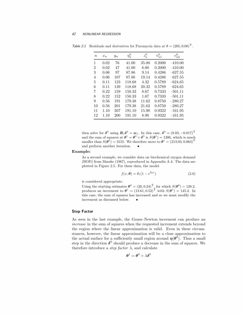
42 NONLINEAR REGRESSION
Table 2.1 Residuals and derivatives for Puromycin data at θ = (205, 0.08)T.
n xn yn η0n z0
n v0n1 v0
n2
1 0.02 76 41.00 35.00 0.2000 –410.002 0.02 47 41.00 6.00 0.2000 –410.003 0.06 97 87.86 9.14 0.4286 –627.554 0.06 107 87.86 19.14 0.4286 –627.555 0.11 123 118.68 4.32 0.5789 –624.656 0.11 139 118.68 20.32 0.5789 –624.657 0.22 159 150.33 8.67 0.7333 –501.118 0.22 152 150.33 1.67 0.7333 –501.119 0.56 191 179.38 11.62 0.8750 –280.2710 0.56 201 179.38 21.62 0.8750 –280.2711 1.10 207 191.10 15.90 0.9322 –161.9512 1.10 200 191.10 8.90 0.9322 –161.95
then solve for δ0 using R1δ0 = w1. In this case, δ0 = (8.03,−0.017)T
and the sum of squares at θ1 = θ0 + δ0 is S(θ1) = 1206, which is muchsmaller than S(θ0) = 3155. We therefore move to θ1 = (213.03, 0.063)T
and perform another iteration. •Example:
As a second example, we consider data on biochemical oxygen demand(BOD) from Marske (1967), reproduced in Appendix A.4. The data areplotted in Figure 2.5. For these data, the model
f(x, θ) = θ1(1 − eθ2x) (2.8)
is considered appropriate.
Using the starting estimates θ0 = (20, 0.24)T, for which S(θ0) = 128.2,produces an increment to θ1 = (13.61, 0.52)T with S(θ1) = 145.2. Inthis case, the sum of squares has increased and so we must modify theincrement as discussed below. •
Step Factor
As seen in the last example, the Gauss–Newton increment can produce anincrease in the sum of squares when the requested increment extends beyondthe region where the linear approximation is valid. Even in these circum-stances, however, the linear approximation will be a close approximation tothe actual surface for a sufficiently small region around η(θ0). Thus a smallstep in the direction δ0 should produce a decrease in the sum of squares. Wetherefore introduce a step factor λ, and calculate
θ1 = θ0 + λδ0
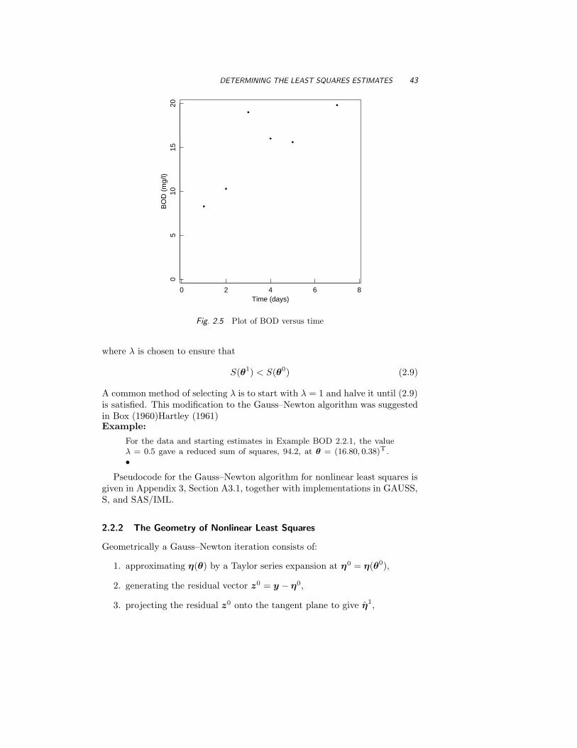
DETERMINING THE LEAST SQUARES ESTIMATES 43
•
•
•
• •
•
Time (days)
BO
D (
mg/
l)
0 2 4 6 8
05
1015
20
Fig. 2.5 Plot of BOD versus time
where λ is chosen to ensure that
S(θ1) < S(θ0) (2.9)
A common method of selecting λ is to start with λ = 1 and halve it until (2.9)is satisfied. This modification to the Gauss–Newton algorithm was suggestedin Box (1960)Hartley (1961)Example:
For the data and starting estimates in Example BOD 2.2.1, the valueλ = 0.5 gave a reduced sum of squares, 94.2, at θ = (16.80, 0.38)T.•
Pseudocode for the Gauss–Newton algorithm for nonlinear least squares isgiven in Appendix 3, Section A3.1, together with implementations in GAUSS,S, and SAS/IML.
2.2.2 The Geometry of Nonlinear Least Squares
Geometrically a Gauss–Newton iteration consists of:
1. approximating η(θ) by a Taylor series expansion at η0 = η(θ0),
2. generating the residual vector z0 = y − η0,
3. projecting the residual z0 onto the tangent plane to give η1,

44 NONLINEAR REGRESSION
η1
η 2
90 100 110 120 130 140 150
6070
8090
100
110
0.01
0.05
0.10.15
•
y •
0.05
0
–0.05
η1^
Fig. 2.6 A geometric interpretation of calculation of the Gauss–Newton incrementusing the 2-case Rumford data. A portion of the expectation surface (heavy solid line)is shown in the response space together with the observed response y. Also shown isthe projection η1 of y − η(0.05) onto the tangent plane at η(0.05) (solid line). Thetick marks indicate true positions on the expectation surface and linear approximationpositions on the tangent plane.
4. mapping η1 through the linear coordinate system to produce the incre-ment δ0, and finally
5. moving to η(θ0 + λδ0).
The first step actually involves two distinct approximations:
1. the planar assumption, in which we approximate the expectation surfaceη(θ) near η(θ0) by its tangent plane at η(θ0), and
2. the uniform coordinate assumption, in which we impose a linear coor-dinate system V (θ − θ0) on the approximating tangent plane.
We give geometrical interpretations of these steps and assumptions in thefollowing examples.Example:
For the 2-case Rumford data set of Example Rumford 2.1.3, we ploty and a portion of the expectation surface in Figure 2.6. The ex-pectation surface is a curved line, and the points corresponding toθ = 0.01, 0.02, . . . , 0.2 are unevenly spaced.
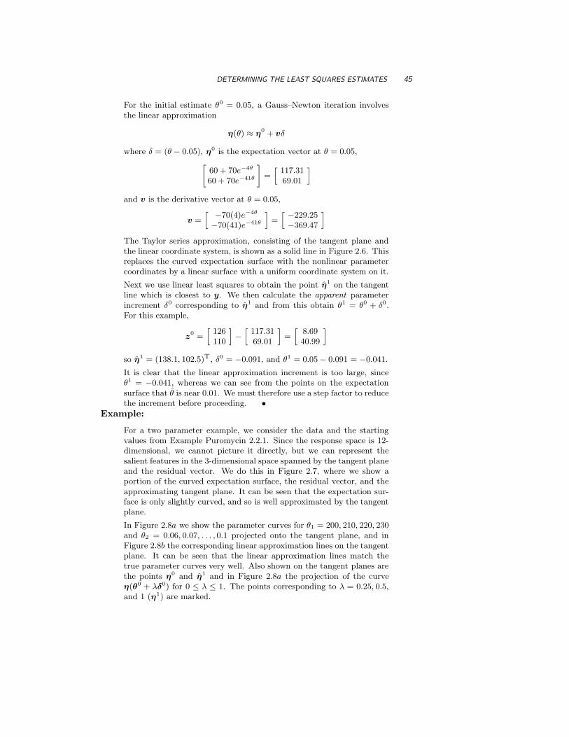
DETERMINING THE LEAST SQUARES ESTIMATES 45
For the initial estimate θ0 = 0.05, a Gauss–Newton iteration involvesthe linear approximation
η(θ) ≈ η0 + vδ
where δ = (θ − 0.05), η0 is the expectation vector at θ = 0.05,
[
60 + 70e−4θ
60 + 70e−41θ
]
=[
117.3169.01
]
and v is the derivative vector at θ = 0.05,
v =[ −70(4)e−4θ
−70(41)e−41θ
]
=[ −229.25−369.47
]
The Taylor series approximation, consisting of the tangent plane andthe linear coordinate system, is shown as a solid line in Figure 2.6. Thisreplaces the curved expectation surface with the nonlinear parametercoordinates by a linear surface with a uniform coordinate system on it.
Next we use linear least squares to obtain the point η1 on the tangentline which is closest to y. We then calculate the apparent parameterincrement δ0 corresponding to η1 and from this obtain θ1 = θ0 + δ0.For this example,
z0 =
[
126110
]
−[
117.3169.01
]
=[
8.6940.99
]
so η1 = (138.1, 102.5)T, δ0 = −0.091, and θ1 = 0.05 − 0.091 = −0.041.
It is clear that the linear approximation increment is too large, sinceθ1 = −0.041, whereas we can see from the points on the expectationsurface that θ is near 0.01. We must therefore use a step factor to reducethe increment before proceeding. •
Example:
For a two parameter example, we consider the data and the startingvalues from Example Puromycin 2.2.1. Since the response space is 12-dimensional, we cannot picture it directly, but we can represent thesalient features in the 3-dimensional space spanned by the tangent planeand the residual vector. We do this in Figure 2.7, where we show aportion of the curved expectation surface, the residual vector, and theapproximating tangent plane. It can be seen that the expectation sur-face is only slightly curved, and so is well approximated by the tangentplane.
In Figure 2.8a we show the parameter curves for θ1 = 200, 210, 220, 230and θ2 = 0.06, 0.07, . . . , 0.1 projected onto the tangent plane, and inFigure 2.8b the corresponding linear approximation lines on the tangentplane. It can be seen that the linear approximation lines match thetrue parameter curves very well. Also shown on the tangent planes arethe points η0 and η1 and in Figure 2.8a the projection of the curveη(θ0 + λδ0) for 0 ≤ λ ≤ 1. The points corresponding to λ = 0.25, 0.5,and 1 (η1) are marked.

46 NONLINEAR REGRESSION
•
•
•
η1^ η0
y
Fig. 2.7 A geometric interpretation of calculation of the Gauss–Newton incrementusing the full Puromycin data set. We show the projection of a portion of the expec-tation surface into the subspace spanned by the tangent plane at η0 (shaded) and theresidual vector y−η0. The region on the expectation surface is bordered by the heavysolid lines. Also shown is the projection η1 of the residual vector onto the tangentplane.
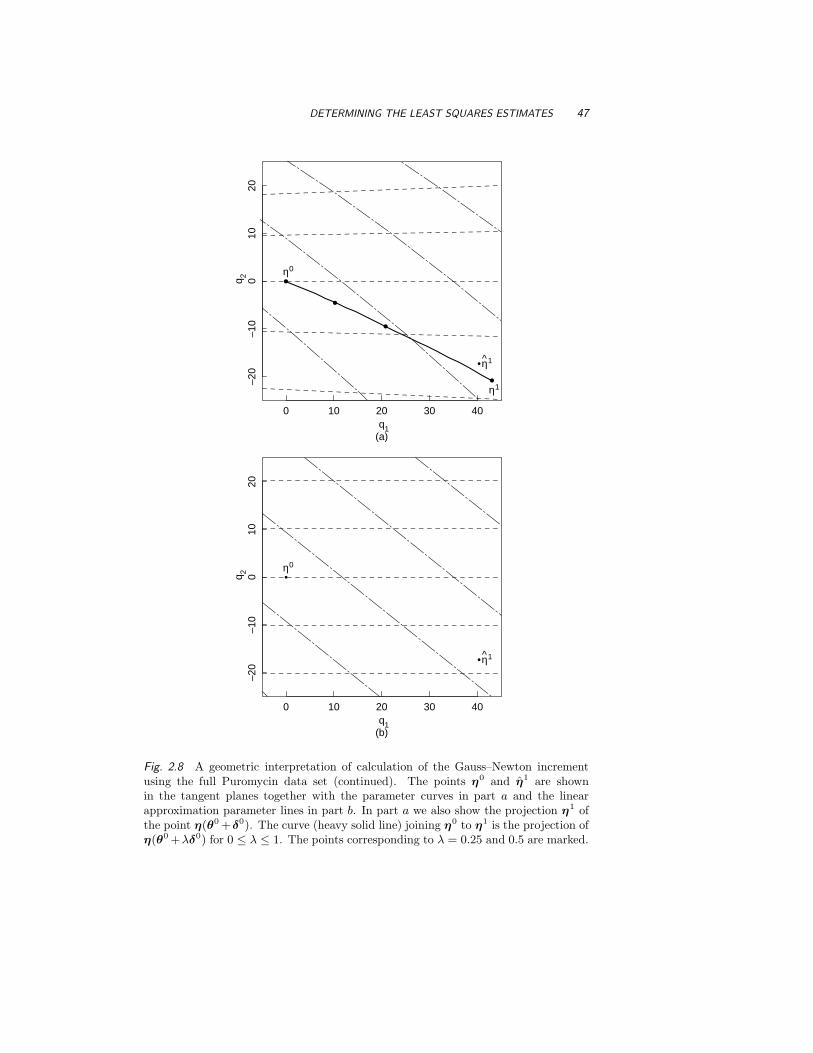
DETERMINING THE LEAST SQUARES ESTIMATES 47
q1
q 2
0 10 20 30 40
–20
–10
010
20
(a)
•
•
η1 ^
η0
••
•
•η1
q1
q 2
0 10 20 30 40
–20
–10
010
20
(b)
•
•
η1 ^
η0
Fig. 2.8 A geometric interpretation of calculation of the Gauss–Newton incrementusing the full Puromycin data set (continued). The points η0 and η1 are shownin the tangent planes together with the parameter curves in part a and the linearapproximation parameter lines in part b. In part a we also show the projection η1 ofthe point η(θ0 +δ0). The curve (heavy solid line) joining η0 to η1 is the projection ofη(θ0 +λδ0) for 0 ≤ λ ≤ 1. The points corresponding to λ = 0.25 and 0.5 are marked.

48 NONLINEAR REGRESSION
•
•
•
η0
y
η1 ^
Fig. 2.9 A geometric interpretation of calculation of the Gauss–Newton incrementusing the BOD data set. We show the projection of a portion of the expectation surfaceinto the subspace spanned by the tangent plane at η0 (shaded) and the residual vectory − η0. The region on the expectation surface is bordered by the heavy solid lines.Also shown is the projection η1 of the residual vector onto the tangent plane.
Because the planar and uniform coordinate assumptions are both valid,the points η1 and η1 are close together and are much closer to y thanη0. In this case, a full step (λ = 1) can be taken resulting in a decreasein the sum of squares as shown in Example Puromycin 2.2.1. •
Example:
As a second two-parameter example, we consider the data and startingvalues from Example BOD 2.2.1. In Figure 2.9 we show a portion of thecurved expectation surface, the residual vector, and the approximatingtangent plane in the space spanned by the tangent plane and the residualvector. It can be seen that the expectation surface is moderately curved,but is still apparently well approximated by the tangent plane. In thisexample, the edge of the finite expectation surface is shown as the angledsolid line along the top edge of the surface.
In Figure 2.10a we show the parameter curves for θ1 = 20, 30, . . . andθ2 = 0.2, 0.4, . . . projected onto the tangent plane. In Figure 2.10bwe show the corresponding linear approximation lines on the tangentplane. In this case, the linear approximation lines do not match thetrue parameter curves well at all. Also shown on the tangent planes arethe points η0 and η1, and in Figure 2.10a the projection of the curve

DETERMINING THE LEAST SQUARES ESTIMATES 49
q1
q 2
–4 –2 0 2 4 6 8 10
–4–2
02
46
810
(a)
•
•
η1 ^
η0•••
• η1
q1
q 2
–4 –2 0 2 4 6 8 10
–4–2
02
46
810
(b)
•
•
η1 ^
η0
Fig. 2.10 A geometric interpretation of calculation of the Gauss–Newton incrementusing the BOD data set (continued). The points η0and η1 are shown in the tangentplanes together with the parameter curves in part a and the linear approximationparameter lines in part b. In part a we also show the projection η1 of the pointη(θ0+δ0). The curve (heavy solid line) joining η0 to η1 is the projection of η(θ0+λδ0)for 0 ≤ λ ≤ 1. The points corresponding to λ = 0.25 and 0.5 are marked.
50 NONLINEAR REGRESSION
η(θ0 + λδ0) for 0 ≤ λ ≤ 1. The points corresponding to λ = 0.25, 0.5,and 1 (η1) are marked.
Because the uniform coordinate assumption is not valid this far fromθ0, the points η1 and η1 are widely separated, and in fact η1 is fartherfrom η1 than is η0. In this case, the reduced step, λ = 0.5, is successful,as was shown in Example BOD 2.2.1. •
To summarize, geometrically we are using local information to generate atangent plane with a linear coordinate system dictated by the derivative vec-tors, projecting the residual vector onto that tangent plane, and then mappingthe tangent plane coordinates to the parameter plane using the linear map-ping.
2.2.3 Convergence
We have indicated that the Gauss–Newton iterative method is continued untilthe values of θ on successive iterations stabilize. This can be measured bythe size of each parameter increment relative to the previous parameter value,which is the basis for one of the common criteria used to declare convergence(Bard, 1974; Draper and Smith, 1981; Jennrich and Sampson, 1968; Ralstonand Jennrich, 1978; Kennedy, Jr. and Gentle, 1980). Another criterion forconvergence used, for example, in SAS (SAS, 1985), is that the relative changein the sum of squares on successive iterations be small. Himmelblau (1972)recommends that both these criteria be used, since compliance with one doesnot imply compliance with the other. However, compliance even with bothrelative change criteria does not guarantee convergence, as discussed in Batesand Watts (1981). Kennedy, Jr. and Gentle (1980) mention a relative stepsize criterion as well as relative change in the sum of squares and gradientsize criteria. Chambers (1977) quotes several other criteria, including the sizeof the gradient, the size of the Gauss–Newton step, and the fact that theresidual vector should be orthogonal to the derivative vectors; but no scale issuggested.
The main criticism of these criteria is that they indicate lack of progressrather than convergence. In most cases, of course, lack of progress occursbecause a minimum is encountered: nevertheless, situations can occur wherethe parameter increment and sum of squares convergence criteria indicate lackof progress and yet a minimum has not been reached.
Examination of the geometry of nonlinear least squares provides a betterprocedure for determining convergence (Bates and Watts, 1981b). We knowthat a critical point is reached whenever the residual vector y − η(θ) is or-thogonal to the expectation surface and therefore to the tangent plane to theexpectation surface at η(θ). We can thus adopt orthogonality of the residualvector to the tangent plane as a convergence criterion.
In practice, it would be unusual to obtain exact orthogonality in the pres-ence of numerical roundoff, and we do not want to waste effort calculatingsmall changes in the parameter vector while trying to achieve perfect orthog-
DETERMINING THE LEAST SQUARES ESTIMATES 51
onality. We therefore need to establish a tolerance level which we can use todeclare the residual vector to be “sufficiently orthogonal.” One way to do thisis to consider the statistical variability in the least squares estimates.
If we assume that the tangent plane forms a good approximation to theexpectation surface near θ, so a likelihood region for θ roughly corresponds
to a disk on the tangent plane with a radius proportional to
√
S(θ), then wecan measure the relative offset of the current parameter values from the exactleast squares estimates by calculating the ratio of the length of the component
of the residual vector in the tangent plane to
√
S(θ). When this ratio is small,the numerical uncertainty of the least squares estimates is negligible comparedto the statistical uncertainty of the parameters.
Unfortunately, this criterion involves the unknown least squares vector θ.We therefore modify the criterion by substituting the current estimate, θi,for θ, and measure the scaled length of the tangent plane component of theresidual vector relative to the scaled length of the orthogonal component ofthe residual vector at θi. This leads to a relative offset convergence criterion
‖QT1 (y − η(θi))‖/
√P
‖QT2 (y − η(θi))‖/
√N − P
(2.10)
where Q1 and Q2 are the first P and last N − P columns respectively of thematrix Q from a QR decomposition of V . The criterion is related to thecotangent of the angle that the residual vector makes with the tangent plane,so that a small relative offset corresponds to an angle near 90◦.
To declare convergence, we require the relative offset to be less than 0.001,reasoning that any inferences will not be affected materially by the fact thatthe current parameter vector is less than 0.1% of the radius of the confidenceregion disk from the least squares point.Example:
We illustrate the convergence criterion and its development with the 2-observation Rumford example. We wish to test whether the parametervalue θ = 0.01 could be considered a point of convergence. Figure2.11 shows a portion of the expectation surface, the observation pointy, and the tangent plane at η(0.01). Also shown is the componentof the residual vector in the tangent plane, QT
1 z, and the componentorthogonal to the tangent plane, QT
2 z. The tangent plane componentis large relative to the orthogonal component, having a relative offsetof 1.92, and so we conclude that the residual vector at θ = 0.01 is notsufficiently orthogonal for us to accept θ = 0.01 as the converged value.
•Convergence implies that the best estimates of the parameters have been
obtained, under the assumption that the model is adequate. Before char-acterizing the precision of the estimates using inference intervals or regions,therefore, we should check the residuals for signs of model inadequacy. Acomplete discussion of the practical aspects of nonlinear regression is given in

52 NONLINEAR REGRESSION
η1
η 2
125 126 127 128 129
106
107
108
109
110
•
y •
0.008
0.01
Q2Tz
Q1Tz
z
Fig. 2.11 A geometric interpretation of relative offset using the 2-case Rumford data.A portion of the expectation surface (dashed line) is shown in the expectation spacetogether with the residual vector z and its projections into the tangent plane (QT
1 z)and orthogonal to the tangent plane (QT
2 z).
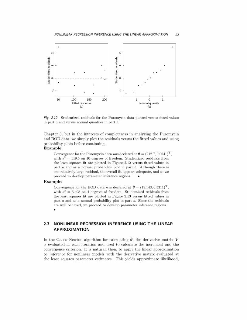
NONLINEAR REGRESSION INFERENCE USING THE LINEAR APPROXIMATION 53
•
••
•
•
•
•
•
•
•
•
•
Fitted response
Stu
dent
ized
res
idua
ls
50 100 150 200
–10
12
(a)
• •
• ••
• •
• ••
•
•
Normal quantile
Stu
dent
ized
res
idua
ls
–1 0 1
–10
12
(b)
Fig. 2.12 Studentized residuals for the Puromycin data plotted versus fitted valuesin part a and versus normal quantiles in part b.
Chapter 3, but in the interests of completeness in analyzing the Puromycinand BOD data, we simply plot the residuals versus the fitted values and usingprobability plots before continuing.Example:
Convergence for the Puromycin data was declared at θ = (212.7, 0.0641)T ,with s2 = 119.5 on 10 degrees of freedom. Studentized residuals fromthe least squares fit are plotted in Figure 2.12 versus fitted values inpart a and as a normal probability plot in part b. Although there isone relatively large residual, the overall fit appears adequate, and so weproceed to develop parameter inference regions. •
Example:
Convergence for the BOD data was declared at θ = (19.143, 0.5311)T ,with s2 = 6.498 on 4 degrees of freedom. Studentized residuals fromthe least squares fit are plotted in Figure 2.13 versus fitted values inpart a and as a normal probability plot in part b. Since the residualsare well behaved, we proceed to develop parameter inference regions.•
2.3 NONLINEAR REGRESSION INFERENCE USING THE LINEAR
APPROXIMATION
In the Gauss–Newton algorithm for calculating θ, the derivative matrix V
is evaluated at each iteration and used to calculate the increment and theconvergence criterion. It is natural, then, to apply the linear approximationto inference for nonlinear models with the derivative matrix evaluated atthe least squares parameter estimates. This yields approximate likelihood,
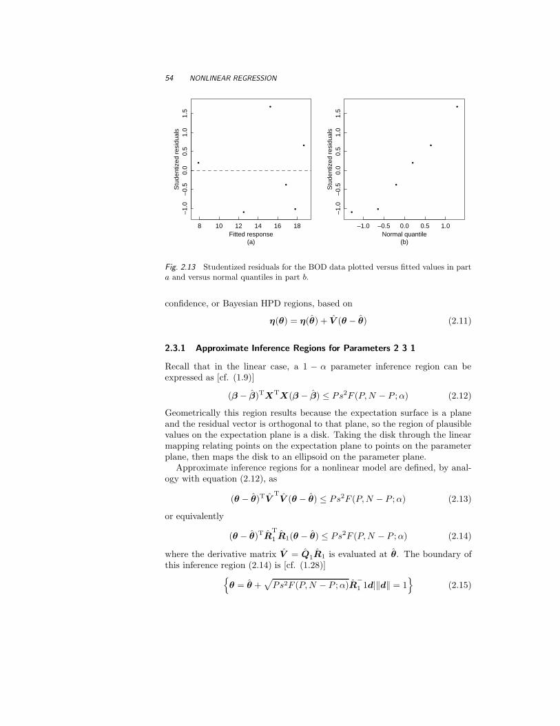
54 NONLINEAR REGRESSION
•
•
•
•
•
•
Fitted response
Stu
dent
ized
res
idua
ls
8 10 12 14 16 18
–1.0
–0.5
0.0
0.5
1.0
1.5
(a)
• •
•
•
•
•
Normal quantile
Stu
dent
ized
res
idua
ls
–1.0 –0.5 0.0 0.5 1.0
–1.0
–0.5
0.0
0.5
1.0
1.5
(b)
Fig. 2.13 Studentized residuals for the BOD data plotted versus fitted values in parta and versus normal quantiles in part b.
confidence, or Bayesian HPD regions, based on
η(θ) = η(θ) + V (θ − θ) (2.11)
2.3.1 Approximate Inference Regions for Parameters 2 3 1
Recall that in the linear case, a 1 − α parameter inference region can beexpressed as [cf. (1.9)]
(β − β)TXTX(β − β) ≤ Ps2F (P, N − P ; α) (2.12)
Geometrically this region results because the expectation surface is a planeand the residual vector is orthogonal to that plane, so the region of plausiblevalues on the expectation plane is a disk. Taking the disk through the linearmapping relating points on the expectation plane to points on the parameterplane, then maps the disk to an ellipsoid on the parameter plane.
Approximate inference regions for a nonlinear model are defined, by anal-ogy with equation (2.12), as
(θ − θ)TVTV (θ − θ) ≤ Ps2F (P, N − P ; α) (2.13)
or equivalently
(θ − θ)TRT
1 R1(θ − θ) ≤ Ps2F (P, N − P ; α) (2.14)
where the derivative matrix V = Q1R1 is evaluated at θ. The boundary ofthis inference region (2.14) is [cf. (1.28)]
{
θ = θ +√
Ps2F (P, N − P ; α)R−
1 1d|‖d‖ = 1}
(2.15)

INFERENCE USING LINEAR APPROXIMATION 55
θ1
θ 2
190 200 210 220 230 240
0.04
0.06
0.08
0.10
+
Fig. 2.14 Parameter approximate inference regions for the Puromycin data. We showthe least squares estimates (+), the parameter joint 95 and 99% inference regions(solid lines), and the marginal 95% inference intervals (dashed lines).
Similarly, the approximate standard error for θp is s times the length of
the pth row of R−
1 1’-1p’ [cf. (1.33)]. Approximate correlations and standard
errors for the parameters are easily calculated by factoring R−1 into a diagonal
matrix [cf. (1.34)] giving the lengths of the rows of R−
1 and a matrix withunit length rows as described in Section 1.2.3. The parameter approximatecorrelation matrix is calculated as in (1.35).Example:
Convergence for the Puromycin data was declared at θ = (212.7, 0.0641)T ,with s2 = 119.5 on 10 degrees of freedom and
R1 =[ −2.4441
01568.71320.3
]
The 95 and 99% approximate joint inference regions were obtained byevaluating (2.15) with d = (cos ω, sin ω)T and are plotted in Figure2.14. To calculate approximate marginal inference intervals, we factor
R−1
1 =[ −0.4092
00.4861
0.0007574
]
=[
0.63540
00.0007574
] [ −0.64390
0.76511.0000
]
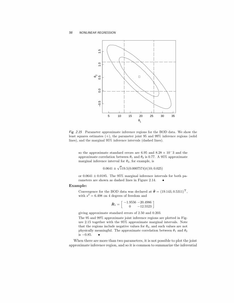
56 NONLINEAR REGRESSION
θ1
θ 2
5 10 15 20 25 30 35
–0.5
0.0
0.5
1.0
1.5
+
Fig. 2.15 Parameter approximate inference regions for the BOD data. We show theleast squares estimates (+), the parameter joint 95 and 99% inference regions (solidlines), and the marginal 95% inference intervals (dashed lines).
so the approximate standard errors are 6.95 and 8.28 × 10⁻³ and theapproximate correlation between θ1 and θ2 is 0.77. A 95% approximatemarginal inference interval for θ2, for example, is
0.0641 ±√
119.5(0.0007574)t(10; 0.025)
or 0.0641 ± 0.0185. The 95% marginal inference intervals for both pa-rameters are shown as dashed lines in Figure 2.14. •
Example:
Convergence for the BOD data was declared at θ = (19.143, 0.5311)T ,with s2 = 6.498 on 4 degrees of freedom and
R1 =[ −1.9556
0−20.4986−12.5523
]
giving approximate standard errors of 2.50 and 0.203.
The 95 and 99% approximate joint inference regions are plotted in Fig-ure 2.15 together with the 95% approximate marginal intervals. Notethat the regions include negative values for θ2, and such values are notphysically meaningful. The approximate correlation between θ1 and θ2
is −0.85. •When there are more than two parameters, it is not possible to plot the joint
approximate inference region, and so it is common to summarize the inferential

INFERENCE USING LINEAR APPROXIMATION 57
•
•
•
•
• •
• ••
•
•
••
•
••••
•
•
•
•
•
•
Hydrogen partial pressure (psia)
Rea
ctio
n ra
te (
hr–1
)
100 200 300 400
02
46
810
12
(a)
•
•
•
•
• •
•••
•
•
••
•
••••
•
•
•
•
•
•
n-Pentane partial pressure (psia)
Rea
ctio
n ra
te (
hr–1
)
100 150 200 250 300
02
46
810
12
(b)
•
•
•
•
• •
•••
•
•
••
•
••••
•
•
•
•
•
•
Isopentane partial pressure (psia)
Rea
ctio
n ra
te (
hr–1
)
50 100 150
02
46
810
12
(c)
Fig. 2.16 Plots of reaction rate of the isomerization of n-pentane to isopentane versusthe partial pressures of hydrogen in part a, n-pentane in part b, and isopentane in partc.
situation by quoting the approximate marginal inference intervals and theparameter correlation matrix and by making pairwise plots of the inferenceregion. More exact methods for summarizing the inferential situtation arepresented in Chapter 6.Example:
Data on the reaction rate of the catalytic isomerization of n-pentaneto isopentane versus the partial pressures of hydrogen, n-pentane, andisopentane as given in Carr (1960)Appendix A, Section A.5, and plottedin Figure 2.16. A proposed model function for these data is
f(x, θ) =θ1θ3(x2 − x3/1.632)
1 + θ2x1 + θ3x2 + θ4x3(2.16)
58 NONLINEAR REGRESSION
Table 2.2 Parameter summary for the isomerization data
Parameter estimates and summary statistics are given in Table 2.2,and residual plots versus the partial pressures and the fitted values inFigure 2.17. The plots show the residuals are generally well behaved.The summary statistics suggest potential difficulties, since some of thecorrelations are extremely high and some of the standard errors pro-duce approximate 95% intervals which include negative values, but theparameters must be positive to be physically meaningful. The pair-wise plots of the parameter approximate 95% inference region, given inFigure 2.18, clearly extend into negative parameter regions. •
2.3.2 Approximate Inference Bands for the Expected Response
Linear approximation inference intervals and bands for the expected responsein nonlinear regression can be generated using the analogs of the equationfor linear regression, (1.11) and (1.12). In those equations, we simply replace
the estimated value xT0 β by f(x0, θ), the matrix X by V , and the derivative
vector x0 by
v0 =∂f(x0, θ)
∂θT
∣
∣
∣
∣
θ
The 1 − α approximate inference interval is then
f(x0, θ) ± s‖vT0 R
−1
1 ‖t(N − P ; α/2) [cf.(1.36)]
and the 1 − α approximate inference band is
f(x, θ) ± s‖vTR−1
1 ‖√
PF (P, N − P ; α) [cf.(1.37)]
Example:
For the Puromycin data, the estimated response at x = 0.4 is 183.3
and the derivative vector is v = (0.8618,−394.9)T , so that, using R−1
1
from Example Puromycin 6, vTR−1
1 = (−0.3526, 0.1198). The inferenceband at x = 0.4 is then (171.6, 195.0). A plot of the approximate 95%inference band is given in Figure 2.19. The band gradually widens fromzero width at x = 0 to a constant width as x → ∞. •
Example:
The estimated response function for the BOD data and the approximate95% inference band is plotted in Figure 2.20. The band widens from zero
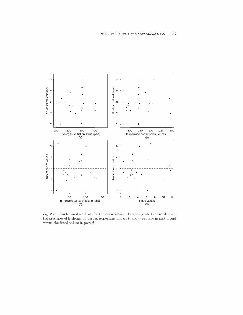
INFERENCE USING LINEAR APPROXIMATION 59
••
•
••
••
•
•
•
•
•
•
•
•
•
•
•
•
••
•
•
•
Hydrogen partial pressure (psia)
Stu
dent
ized
res
idua
ls
100 200 300 400
–2–1
01
2
(a)
••
•
••
• •
•
•
•
•
•
•
•
•
•
•
•
•
••
•
•
•
Isopentane partial pressure (psia)
Stu
dent
ized
res
idua
ls
100 150 200 250 300
–2–1
01
2
(b)
••
•
••
• •
•
•
•
•
•
•
•
•
•
•
•
•
••
•
•
•
n-Pentane partial pressure (psia)
Stu
dent
ized
res
idua
ls
50 100 150
–2–1
01
2
(c)
••
•
••
• •
•
•
•
•
•
•
•
•
•
•
•
•
••
•
•
•
Fitted values
Stu
dent
ized
res
idua
ls
0 2 4 6 8 10 12
–2–1
01
2
(d)
Fig. 2.17 Studentized residuals for the isomerization data are plotted versus the par-tial pressures of hydrogen in part a, isopentane in part b, and n-pentane in part c, andversus the fitted values in part d.

60 NONLINEAR REGRESSION
+
+ +
+ + +
25 30 35 40 45
θ1
–0.1 0.1 0.2 0.3
θ2
–0.10 0.0 0.10
θ3
–0.1
0.1
0.2
0.3
θ 2
–0.1
00.
00.
10
θ 3
–0.4
0.0
0.4
θ 4
Fig. 2.18 Pairwise plots of the parameter approximate 95% inference region for theisomerization data. For each pair of parameters we show the least squares estimates(+), the parameter approximate joint 95% inference region (solid line), and the ap-proximate marginal 95% inference intervals (dotted lines).

INFERENCE USING LINEAR APPROXIMATION 61
0.0 0.2 0.4 0.6 0.8 1.0 1.2
050
100
150
200
250
•
•
••
•
•
••
•• •
•
Concentration
Vel
ocity
Fig. 2.19 Approximate 95% inference band for the Puromycin data. The fitted ex-pectation function is shown as a solid line, and the 95% inference band is shown as apair of dotted lines.
0 2 4 6 8
–50
510
1520
2530
••
•
• •
•
Time
Oxy
gen
dem
and
Fig. 2.20 Approximate 95% inference band for the BOD data. The fitted expectationfunction is shown as a solid line, and the 95% inference band is shown as a pair ofdotted lines.

62 NONLINEAR REGRESSION
width at x = 0, narrows around x = 4 and then gradually approachesa constant width as x → ∞. •
Inference bands for nonlinear models behave quite differently from thosefor linear models. In the above examples, because the functions are con-strained to go through the origin, the bands reduce to 0 there. Also, becausethe model functions approach horizontal asymptotes, the inference bands ap-proach asymptotes. These characteristics differ from those of the inferencebands for linear models as exemplified in Figure 1.3. There it is seen that thebands are narrowest near the middle of the data, and expand without limit.
2.4 NONLINEAR LEAST SQUARES VIA SUMS OF SQUARES
Sums of squares occur explicitly in linear and nonlinear least squares becauseof the assumptions of normality, independence, and constant variance of thedisturbances. It is therefore natural to view linear and nonlinear regressionvia sums of squares, which can help in understanding these two topics. Thelikelihood approach is especially closely linked to sum of squares contours, be-cause the loglikelihood function is directly proportional to the sum of squaresfunction S(θ).
An important characteristic of linear models is that the sum of squaresfunction S(β) is quadratic. Because of this, contours of constant sums ofsquares are well-behaved regular curves or surfaces, such as ellipses and ellip-soids, and so the loglikelihood function can be completely summarized by:
• the minimum value of the sum of squares function, S(β),
• the location of the minimum of the sum of squares function, β, and
• the second derivative (Hessian) of the sum of squares function,
∂2S(β)
∂β∂βT= XTX
Furthermore, all these quantities can be determined analytically. For non-linear models, however, the sum of squares function is not regular or wellbehaved, and so it is difficult to summarize the loglikelihood function.
2.4.1 The Linear Approximation
Linear approximations of the expectation function are used to determine incre-ments while seeking the least squares estimates, and to determine approximateinference regions when convergence has been achieved. The linear approxi-mation to η(θ) based at θ0, (2.6), produces a linear approximation to theresidual vector z(θ), (2.7), and hence a quadratic approximation S(θ) to the

NONLINEAR LEAST SQUARES VIA SUMS OF SQUARES 63
sum of squares function S(θ), since
S(θ) = ‖y − η(θ)‖2 (2.17)
= z(θ)Tz(θ) ≈ S(θ)
= [z0 − V 0(θ − θ0)]T[z0 − V 0(θ − θ0)]
= z0Tz0 − 2z0T
V 0(θ − θ0) + (θ − θ0)TV 0TV 0(θ − θ0)
= S(θ0) − 2[y − η(θ0)]TV 0(θ − θ0) + (θ − θ0)TV 0TV 0(θ − θ0)(2.18)
The location of the minimum of S(θ) is
θ1 = θ0 + (V 0TV 0)−1V 0T
z0
which gives the Gauss–Newton increment.Note that the quadratic approximation (2.17) is not the second order Taylor
series approximation to S(θ) based at θ0. The Hessian in the Taylor seriesapproximation includes a term involving the second order partial derivativesof the model function with respect to the parameters (see Section 3.5.1).
Contours of the approximate sum of squares function (2.17) are ellipsoidscentered at θ1 and of the form
(θ − θ1)TV 0TV 0(θ − θ1) = c
Of particular interest is the approximating contour
(θ − θ1)TV 0TV 0(θ − θ1) = z0T
V 0(V 0TV 0)−1V 0T
z0
which passes through θ0. If this contour is close to the actual sum of squarescontour which passes through θ0, then we can expect that θ1 will be close tothe optimal value of θ.Example:
In Figure 2.21 we plot the sum of squares function, S(θ), for the Rum-ford data as a solid line. Superimposed on the plot is the approximatingquadratic, S(θ), obtained by taking a linear Taylor series approximationto the expectation function at θ0 = 0.02, shown as a dashed line.
A careful examination of S(θ) shows that it is not a parabola but isasymmetric, with a steeper rise to the left of the minimum than tothe right. The closeness of S(θ) to a parabola indicates the small de-gree of nonlinearity of this model–data set combination. The minimumof the approximating parabola is at 0.008, and so the Gauss–Newtonincrement is 0.008 − 0.02 = −0.012. •
Example:
In Figure 2.22 we plot sum of squares contours, S(θ), for the Puromycindata, shown as solid lines, and the location of the minimum, shown as+. Also shown, as a dashed line, is the ellipse derived from the linearapproximation to the expectation function at θ0 = (205, 0.08)T. The

64 NONLINEAR REGRESSION
θ
S(θ
)
0.0 0.005 0.010 0.015 0.020 0.025 0.030
010
0020
0030
0040
0050
00
•
Fig. 2.21 Sum of squares function for the Rumford data. The true sum of squarescurve is shown as a solid line, and the parabola from the linear approximation atθ0 = 0.02 is shown as a dashed line.
approximating paraboloid has the same value and curvature at θ0 asthe true sum of squares surface, and so the location of the minimumof the paraboloid, denoted by ∗, is used as the apparent minimum ofthe true sum of squares surface. The Gauss increment is therefore thevector joining the starting point θ0 to the point indicated by ∗.
Because the model–data set combination is not badly nonlinear, thesums of squares contours are quite elliptical, and the minimum of the ap-proximating paraboloid is near the minimum of the true sum of squaressurface. •
Example:
In Figure 2.23 we plot sum of squares contours, S(θ), for the BOD data,shown as solid lines, and location of the minimum, shown as +. Alsoshown, as a dashed line, is a portion of the ellipse derived from thelinear approximation to the expectation function at θ0 = (20, 0.24)T.The center of the ellipse is indicated by ∗.
In this example, the ellipse is a poor approximation to the true contour.The center of the ellipse is not close to the minimum of the true sum ofsquares surface and furthermore has a true sum of squares greater thanthat at θ0. •

NONLINEAR LEAST SQUARES VIA SUMS OF SQUARES 65
180 190 200 210 220 230 240 250
0.02
0.04
0.06
0.08
0.10
0.12
•
∗
θ1
θ 2
Fig. 2.22 Sum of squares contours for the Puromycin data. True sum of squarescontours are shown as solid lines, and the elliptical approximate contour from thelinear approximation at θ0 = (205, 0.08)T is shown as a dashed line. The location ofthe minimum sum of squares (+) and the center of the ellipse (∗) are also shown. Thedotted line is the Gauss–Newton increment.
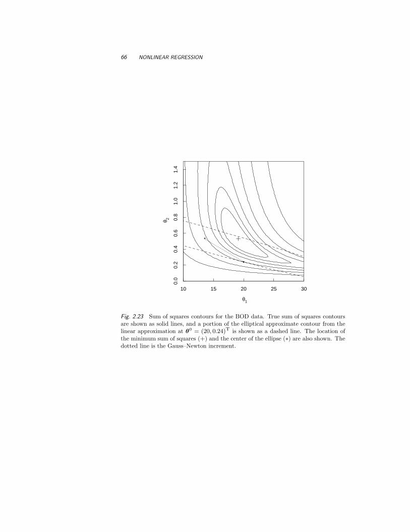
66 NONLINEAR REGRESSION
10 15 20 25 30
0.0
0.2
0.4
0.6
0.8
1.0
1.2
1.4
•
∗
θ1
θ 2
Fig. 2.23 Sum of squares contours for the BOD data. True sum of squares contoursare shown as solid lines, and a portion of the elliptical approximate contour from thelinear approximation at θ0 = (20, 0.24)T is shown as a dashed line. The location ofthe minimum sum of squares (+) and the center of the ellipse (∗) are also shown. Thedotted line is the Gauss–Newton increment.

PROBLEMS 67
2.4.2 Overshoot
The next iteration is carried out from the location of the apparent minimumof the sum of squares surface—provided, of course, that S(θ1) is less thanS(θ0). In the Rumford example and in the Puromycin example, because thenonlinearity is moderate, the sum of squares at θ1 is less than that at θ0,and so we can proceed to iterate from θ1. For the BOD example, however,the sum of squares at θ1 is greater than that at θ0, so we have overshotthe minimum. By incorporating a step factor, so that only a fraction of theincrement is used, we can find a point with a smaller sum of squares, asdescribed in Section 2.2.1.
Problems
2.1 Write a computer routine in a language of your choice to perform non-linear least squares using the Gauss–Newton approach. Take the function, itsderivatives with respect to the parameters, and starting values as input tothe routine. If necessary, use the pseudocode in Appendix 3, Section A3.1 forguidance.
2.2 Use a nonlinear least squares routine to fit a model of the form β1 +β2(age)α to the ln(PCB) data. Use starting values of (−2.4, 2.3, 0.33)T (theleast squares estimates for β1, β2 for α = 0.33 from Example PCB 2).
2.3
2.3.1. Plot the expectation surface for the Rumford model, using the de-sign x = (7, 28)T. Mark the points on the expectation surface correspondingto the values θ = 0, 0.01, . . . , 0.1, 0.2, . . . , 1.0,∞. Compare this expectationsurface with the one based on the design x = (4, 41)T plotted in Figure 2.3.Which design has smaller overall intrinsic nonlinearity? Which design hassmaller overall parameter effects nonlinearity?
2.3.2. Plot the expectation surface for the Rumford model, using the de-sign x = (12, 14)T. Mark the points on the expectation surface correspondingto the values θ = 0, 0.01, . . . , 0.1, 0.2, . . . , 1.0,∞. Compare this expectationsurface with the one based on the design x = (4, 41)T plotted in Figure 2.3and with that from part (a). Which design has smallest overall intrinsic non-linearity? Which design has smallest overall parameter effects nonlinearity?
2.3.3. What kind of design would have zero intrinsic nonlinearity every-where? Why?
2.3.4. Would the design in part (c) have zero parameter effects nonlinear-ity? Why?
2.4
2.4.1. Plot the expectation surface for the linear model ln(PCB) = β ln(age)for the design age = 5, 10. Mark the points on the surface corresponding toβ = 0, 1, 2, 3.

68 NONLINEAR REGRESSION
2.4.2. Compare this expectation surface and its properties with those ofthe nonlinear Rumford model shown in Figure 2.3.
2.4.3. Compare this expectation surface and its properties with those ofthe nonlinear Rumford model plotted in Problem 2.3.
2.5
2.5.1. Generate the expectation vector, the residual vector, the sum ofsquares S(θ0), and the derivative matrix V 0 for the data and model fromAppendix 4, Section A4.1, at the starting values θ0 = (2.20, 0.26)T.
2.5.2. Calculate the increment δ0 and S(θ1), where θ1 = θ0 + λδ0, forλ = 0.25, 0.50, and 1.0. Is a step factor less than 1 necessary in this case?
2.6
2.6.1. Use the fact that, for the model in Problem 2.5, θ1 is conditionallylinear, and generate and plot exact sum of squares contours for the datain Appendix 4, Section A4.1. (That is, for any specified value of θ2, it ispossible to use linear least squares to obtain the conditional estimate θ1 andto calculate the values of θ1 which produce a specified sum of squares. Byspecifying the sum of squares to be that corresponding to a contour value, itis possible to generate the exact coordinates of points on the contour.) Let θ2
go from 0.12 to 0.3 in steps of 0.01, and use contour values corresponding to50, 75, and 95% confidence levels. Mark the location of the minimum on theplot.
2.6.2. Compare these contours with those in Figure 2.23. Which data setsuffers most from nonlinearity?
2.6.3. Since the data are from the same type of experiment with the samemodel, how can this difference be explained?
2.7 Plot the point corresponding to θ0 and the increment δ0 from Problem2.5 on the contour plot from Problem 2.6. Mark the points corresponding tothe values λ = 0.25, 0.5, and 0.75 on the increment vector. Is a step factorless than 1 necessary in this case?
2.8
2.8.1. Use the data, model, and starting values from Problem 2.5 in anonlinear estimation routine to obtain the least squares parameter estimates.
2.8.2. Calculate and plot the linear approximation joint and marginal in-ference regions on the plot from Problem 2.6.
2.8.3. Are the linear approximation inference regions accurate in this case?

Appendix AData Sets Used in
Examples
A.1 PCB
Data on the concentrations of polychlorinated biphenyl (PCB) residues in aseries of lake trout from Cayuga Lake, NY, were reported in Bache et al. (1972)and are reproduced in Table A.1. The ages of the fish were accurately known,because the fish are annually stocked as yearlings and distinctly marked asto year class. Each whole fish was mechanically chopped, ground, and thor-oughly mixed, and 5-gram samples taken. The samples were treated and PCBresidues in parts per million (ppm) were estimated using column chromatog-raphy.
A linear model
f(x, β) = β1 + β2x
is proposed where f is predicted ln(PCB concentration) and x is 3√
age.
69

70 DATA SETS USED IN EXAMPLES
Table A.1 PCB concentration versus age for lake trout.
Age PCB Conc. Age PCB Conc.(years) (ppm) (years) (ppm)
1 0.6 6 3.41 1.6 6 9.71 0.5 6 8.61 1.2 7 4.02 2.0 7 5.52 1.3 7 10.52 2.5 8 17.53 2.2 8 13.43 2.4 8 4.53 1.2 9 30.44 3.5 11 12.44 4.1 12 13.44 5.1 12 26.25 5.7 12 7.4
Copyright 1972 by the AAAS. Reproduced from SCIENCE, 1972, 117,1192–1193, with permission of the authors.
A.2 RUMFORD
Data on the amount of heat generated by friction were obtained by CountRumford in 1798. A bore was fitted into a stationary cylinder and pressedagainst the bottom by means of a screw. The bore was turned by a teamof horses for 30 minutes, after which Rumford “suffered the thermometer toremain in its place nearly three quarters of an hour, observing and notingdown, at small intervals of time, the temperature indicated by it” (Roller,1950). (See Table A.2)
A model based on Newton’s law of cooling was proposed as
f(x, θ) = 60 + 70e−θx
where f is predicted temperature and x is time.
A.3 PUROMYCIN
Data on the “velocity” of an enzymatic reaction were obtained by Treloar(1974). The number of counts per minute of radioactive product from thereaction was measured as a function of substrate concentration in parts permillion (ppm) and from these counts the initial rate, or “velocity,” of the reac-

BOD 71
Table A.2 Temperature versus time for Rumford cooling experiment.
Time Temperature Time Temperature(min) (◦F) (min) (◦F)
4 126 24 1155 125 28 1147 123 31 113
12 120 34 11214 119 37.5 11116 118 41 11020 116
Reprinted with permission from “The Early Development of the Con-cepts of Temperature and Heat: The Rise and Decline of the CaloricTheory.” by Duane Roller, Harvard University Press, 1950.
tion was calculated (counts/min2). The experiment was conducted once withthe enzyme treated with Puromycin, [(a) in Table A.3] and once with the en-zyme untreated (b). The velocity is assumed to depend on the substrate con-centration according to the Michaelis–Menten equation. It was hypothesizedthat the ultimate velocity parameter (θ1) should be affected by introductionof the Puromycin, but not the half-velocity parameter (θ2).
The Michaelis–Menten model is
f(x, θ) =θ1x
θ2+x
where f is predicted velocity and x is substrate concentration.
A.4 BOD
Data on biochemical oxygen demand (BOD) were obtained by Marske (1967).To determine the BOD, a sample of stream water was taken, injected withsoluble organic matter, inorganic nutrients, and dissolved oxygen, and subdi-vided into BOD bottles. Each bottle was innoculated with a mixed culture ofmicroorganisms, sealed, and incubated at constant temperature, and then thebottles were opened periodically and analyzed for dissolved oxygen concen-tration, from which the BOD was calculated in milligrams per liter (mg/l).(See Table A.4) The values shown are the averages of two analyses on eachbottle.
A model was derived based on exponential decay with a fixed rate constantas
f(x, θ) = θ1(1 − eθ2x)
where f is predicted biochemical oxygen demand and x is time.
72 DATA SETS USED IN EXAMPLES
Table A.3 Reaction velocity versus substrate concentration for the Puromycin exper-iment.
Substrate VelocityConcentration (counts/min2)
(ppm) (a) Treated (b) Untreated
0.02 76 6747 51
0.06 97 84107 86
0.11 123 98139 115
0.22 159 131152 124
0.56 191 144201 158
1.10 207 160200
Copyright 1974 by M. A. Treloar. Reproduced from “Effects ofPuromycin on Galactosyltransferase of Golgi Membranes,” Master’sThesis, University of Toronto. Reprinted with permission of the au-thor.
Table A.4 Biochemical oxygen demand versus time.
Biochemical BiochemicalOxygen Oxygen
Time Demand Time Demand(days) (mg/l) (days) (mg/l)
1 8.3 4 16.02 10.3 5 15.63 19.0 7 19.8
Copyright 1967 by D. Marske. Reproduced from “Biochemical Oxy-gen Demand Data Interpretation Using Sum of Squares Surface,”M.Sc. Thesis, University of Wisconsin–Madison. Reprinted with per-mission of the author.

ISOMERIZATION 73
Table A.5 Reaction rate for isomerization of n-pentane to isopentane.
Partial Pressure (psia) ReactionRate
Hydrogen n-Pentane Isopentane (hr−1)
205.8 90.9 37.1 3.541404.8 92.9 36.3 2.397209.7 174.9 49.4 6.694401.6 187.2 44.9 4.722224.9 92.7 116.3 0.593402.6 102.2 128.9 0.268212.7 186.9 134.4 2.797406.2 192.6 134.9 2.451133.3 140.8 87.6 3.196470.9 144.2 86.9 2.021300.0 68.3 81.7 0.896301.6 214.6 101.7 5.084297.3 142.2 10.5 5.686314.0 146.7 157.1 1.193305.7 142.0 86.0 2.648300.1 143.7 90.2 3.303305.4 141.1 87.4 3.054305.2 141.5 87.0 3.302300.1 83.0 66.4 1.271106.6 209.6 33.0 11.648417.2 83.9 32.9 2.002251.0 294.4 41.5 9.604250.3 148.0 14.7 7.754145.1 291.0 50.2 11.590
Copyright 1960 by the American Chemical Society. Reprinted withpermission from Industrial and Engineering Chemistry, 52, 391–396.
A.5 ISOMERIZATION
Data on the reaction rate of the catalytic isomerization of n-pentane to isopen-tane versus the partial pressures of hydrogen, n-pentane, and isopentane weregiven in Carr (1960) and are reproduced in Table A.5. Isomerization is achemical process in which a complex chemical is converted into more simpleunits, called isomers: catalytic isomerization employs catalysts to speed thereaction. The reaction rate depends on various factors, such as partial pres-sures of the products and the concentration of the catalyst. The differential
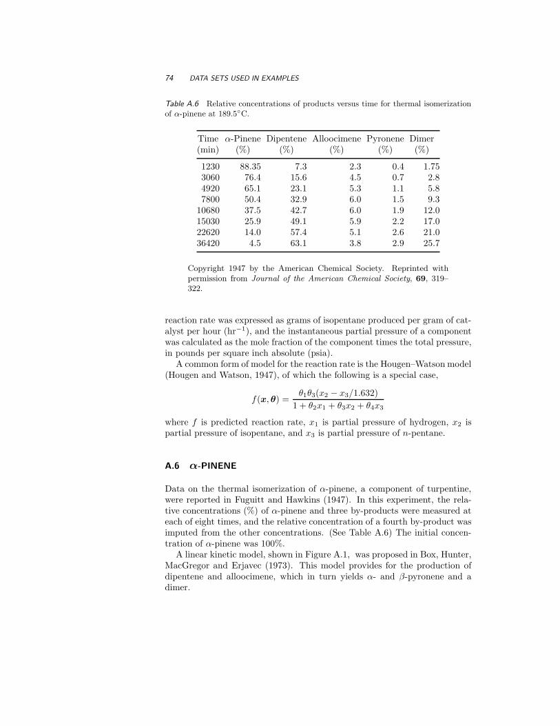
74 DATA SETS USED IN EXAMPLES
Table A.6 Relative concentrations of products versus time for thermal isomerizationof α-pinene at 189.5◦C.
Time α-Pinene Dipentene Alloocimene Pyronene Dimer(min) (%) (%) (%) (%) (%)
1230 88.35 7.3 2.3 0.4 1.753060 76.4 15.6 4.5 0.7 2.84920 65.1 23.1 5.3 1.1 5.87800 50.4 32.9 6.0 1.5 9.3
10680 37.5 42.7 6.0 1.9 12.015030 25.9 49.1 5.9 2.2 17.022620 14.0 57.4 5.1 2.6 21.036420 4.5 63.1 3.8 2.9 25.7
Copyright 1947 by the American Chemical Society. Reprinted withpermission from Journal of the American Chemical Society, 69, 319–322.
reaction rate was expressed as grams of isopentane produced per gram of cat-alyst per hour (hr−1), and the instantaneous partial pressure of a componentwas calculated as the mole fraction of the component times the total pressure,in pounds per square inch absolute (psia).
A common form of model for the reaction rate is the Hougen–Watson model(Hougen and Watson, 1947), of which the following is a special case,
f(x, θ) =θ1θ3(x2 − x3/1.632)
1 + θ2x1 + θ3x2 + θ4x3
where f is predicted reaction rate, x1 is partial pressure of hydrogen, x2 ispartial pressure of isopentane, and x3 is partial pressure of n-pentane.
A.6 α-PINENE
Data on the thermal isomerization of α-pinene, a component of turpentine,were reported in Fuguitt and Hawkins (1947). In this experiment, the rela-tive concentrations (%) of α-pinene and three by-products were measured ateach of eight times, and the relative concentration of a fourth by-product wasimputed from the other concentrations. (See Table A.6) The initial concen-tration of α-pinene was 100%.
A linear kinetic model, shown in Figure A.1, was proposed in Box, Hunter,MacGregor and Erjavec (1973). This model provides for the production ofdipentene and alloocimene, which in turn yields α- and β-pyronene and adimer.
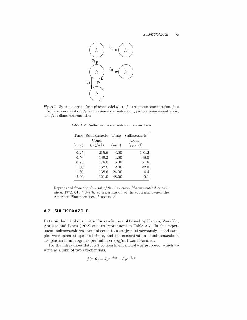
SULFISOXAZOLE 75
f1 f2
f3 f4
f5
θ1
θ2
θ3
θ4 θ5
Fig. A.1 System diagram for α-pinene model where f1 is α-pinene concentration, f2 isdipentene concentration, f3 is alloocimene concentration, f4 is pyronene concentration,and f5 is dimer concentration.
Table A.7 Sulfisoxazole concentration versus time.
Time Sulfisoxazole Time SulfisoxazoleConc. Conc.
(min) (µg/ml) (min) (µg/ml)
0.25 215.6 3.00 101.20.50 189.2 4.00 88.00.75 176.0 6.00 61.61.00 162.8 12.00 22.01.50 138.6 24.00 4.42.00 121.0 48.00 0.1
Reproduced from the Journal of the American Pharmaceutical Associ-
ation, 1972, 61, 773–778, with permission of the copyright owner, theAmerican Pharmaceutical Association.
A.7 SULFISOXAZOLE
Data on the metabolism of sulfisoxazole were obtained by Kaplan, Weinfeld,Abruzzo and Lewis (1972) and are reproduced in Table A.7. In this exper-iment, sulfisoxazole was administered to a subject intravenously, blood sam-ples were taken at specified times, and the concentration of sulfisoxazole inthe plasma in micrograms per milliliter (µg/ml) was measured.
For the intravenous data, a 2-compartment model was proposed, which wewrite as a sum of two exponentials,
f(x, θ) = θ1e−θ2x + θ3e
−θ4x

76 DATA SETS USED IN EXAMPLES
where f is predicted sulfisoxazole concentration and x is time.
A.8 LUBRICANT
Data on the kinematic viscosity of a lubricant, in stokes, as a function oftemperature (◦C), and pressure in atmospheres (atm), were obtained (seeTable A.8) and an empirical model was proposed for the logarithm of theviscosity, as discussed in Linssen (1975).
The proposed model is
f(x, θ) =θ1
θ2 + x1+ θ3x2 + θ4x
22 + θ5x
32 + (θ6 + θ7x
22)x2 exp
( −x1
θ8 + θ9x22
)
where f is predicted ln(viscosity), x1 is temperature, and x2 is pressure.
A.9 CHLORIDE
Data on the rate of transport of sulfite ions from blood cells suspended in asalt solution were obtained by W. H. Dennis and P. Wood at the Universityof Wisconsin, and analyzed by Sredni (1970). The chloride concentration (%)was determined from a continuous curve generated from electrical potentials.(See Table A.9)
A model was derived from the theory of ion transport as
f(x, θ) = θ1(1 − θ2e−θ3x)
where f is predicted chloride concentration and x is time.
A.10 ETHYL ACRYLATE
Data on the metabolism of ethyl acrylate were obtained by giving rats a bo-lus of radioactively tagged ethyl acrylate (Watts, deBethizy and Stiratelli,1986). Each rat was given a measured dose of the compound via stomachintubation and placed in an enclosed cage from which the air could be drawnthrough a bubble chamber. The exhalate was bubbled through the chamber,and at a specified time the bubble chamber was replaced by a fresh one, sothat the measured response was the accumulated CO2 during the collectioninterval. The response reported in Table A.10 is the average, for nine rats, ofthe amount of accumulated CO2 normalized by actual dose, in units of gramsCO2 per gram acrylate per gram rat. An empirical model with three exponen-tial terms was determined from inspection of plots of the data and physicalreasoning. Logarithms of the integrated function were fitted to logarithms ofthe data, using the refinements of Section 3.9.
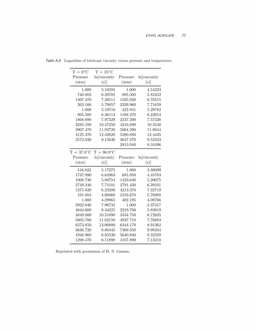
ETHYL ACRYLATE 77
Table A.8 Logarithm of lubricant viscosity versus pressure and temperature.
T = 0◦C T = 25◦CPressure ln[viscosity Pressure ln[viscosity(atm) (s)] (atm) (s)]
1.000 5.10595 1.000 4.54223740.803 6.38705 805.500 5.82452
1407.470 7.38511 1505.920 6.70515363.166 5.79057 2339.960 7.71659
1.000 5.10716 422.941 5.29782805.500 6.36113 1168.370 6.22654
1868.090 7.97329 2237.290 7.573383285.100 10.47250 4216.890 10.35403907.470 11.92720 5064.290 11.98444125.470 12.42620 5280.880 12.44352572.030 9.15630 3647.270 9.52333
2813.940 8.34496
T = 37.8◦C T = 98.9◦CPressure ln[viscosity Pressure ln[viscosity(atm) (s)] (atm) (s)]
516.822 5.17275 1.000 3.380991737.990 6.64963 685.950 4.457831008.730 5.80754 1423.640 5.206752749.240 7.74101 2791.430 6.291011375.820 6.23206 4213.370 7.32719191.084 4.66060 2103.670 5.76988
1.000 4.29865 402.195 4.087662922.940 7.96731 1.000 3.374174044.600 9.34225 2219.700 5.839194849.800 10.51090 3534.750 6.726355605.780 11.82150 4937.710 7.768836273.850 13.06800 6344.170 8.913623636.720 8.80445 7469.350 9.983341948.960 6.85530 5640.940 8.323291298.470 6.11898 4107.890 7.13210
Reprinted with permission of H. N. Linssen.

78 DATA SETS USED IN EXAMPLES
Table A.9 Chloride ion concentration versus time.
Time Conc. Time Conc. Time Conc.(min) (%) (min) (%) (min) (%)
2.45 17.3 4.25 22.6 6.05 26.62.55 17.6 4.35 22.8 6.15 27.02.65 17.9 4.45 23.0 6.25 27.02.75 18.3 4.55 23.2 6.35 27.02.85 18.5 4.65 23.4 6.45 27.02.95 18.9 4.75 23.7 6.55 27.33.05 19.0 4.85 24.0 6.65 27.83.15 19.3 4.95 24.2 6.75 28.13.25 19.8 5.05 24.5 6.85 28.13.35 19.9 5.15 25.0 6.95 28.13.45 20.2 5.25 25.4 7.05 28.43.55 20.5 5.35 25.5 7.15 28.63.65 20.6 5.45 25.9 7.25 29.03.75 21.1 5.55 25.9 7.35 29.23.85 21.5 5.65 26.3 7.45 29.33.95 21.9 5.75 26.2 7.55 29.44.05 22.0 5.85 26.5 7.65 29.44.15 22.3 5.95 26.5 7.75 29.4
Reproduced from J. Sredni, “Problems of Design, Estimation, and Lackof Fit in Model Building,” Ph.D. Thesis, University of Wisconsin–Madison, 1970, with permission of the author.

SACCHARIN 79
Table A.10 Collection intervals and averages of normalized exhaled CO2.
CollectionInterval (hr) CO2
Start Length (g)
0.0 0.25 0.015630.25 0.25 0.041900.5 0.25 0.05328
0.75 0.25 0.052261.0 0.5 0.088501.5 0.5 0.063402.0 2.0 0.134194.0 2.0 0.045026.0 2.0 0.029428.0 16.0 0.02716
24.0 24.0 0.0103748.0 24.0 0.00602
Reproduced with permission.
The integrated model is written
F (x, θ) = −θ4 + θ5
θ1e−θ1x1(1 − e−θ1x2)
+θ4
θ2e−θ2x1(1 − e−θ2x2) +
θ5
θ3e−θ3x1(1 − e−θ3x2)
where F is predicted CO2 exhaled during an interval, x1 is interval startingtime, and x2 is interval duration.
A.11 SACCHARIN
Data on the metabolism of saccharin compounds were obtained by Renwick(1982). In this experiment, a rat received a single bolus of saccharin, and theamount of saccharin excreted was measured by collecting urine in contiguoustime intervals. The measured response was the level of radioactivity of theurine, which was converted to amount of saccharin in micrograms (µg). (SeeTable A.11.) An empirical compartment model with two exponential termswas determined from inspection of plots of the data. Logarithms of the inte-grated function were fitted to logarithms of the data, using the refinements ofSection 3.9.
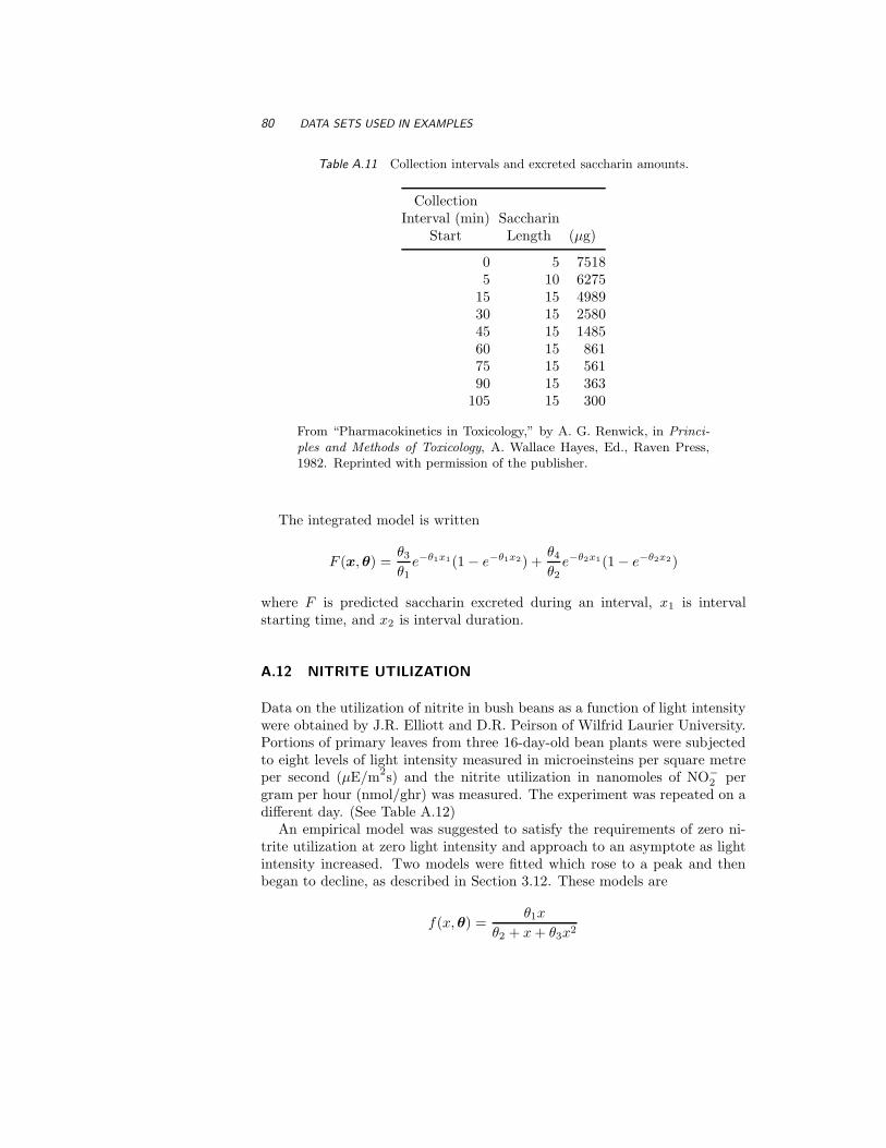
80 DATA SETS USED IN EXAMPLES
Table A.11 Collection intervals and excreted saccharin amounts.
CollectionInterval (min) Saccharin
Start Length (µg)
0 5 75185 10 6275
15 15 498930 15 258045 15 148560 15 86175 15 56190 15 363
105 15 300
From “Pharmacokinetics in Toxicology,” by A. G. Renwick, in Princi-
ples and Methods of Toxicology, A. Wallace Hayes, Ed., Raven Press,1982. Reprinted with permission of the publisher.
The integrated model is written
F (x, θ) =θ3
θ1e−θ1x1(1 − e−θ1x2) +
θ4
θ2e−θ2x1(1 − e−θ2x2)
where F is predicted saccharin excreted during an interval, x1 is intervalstarting time, and x2 is interval duration.
A.12 NITRITE UTILIZATION
Data on the utilization of nitrite in bush beans as a function of light intensitywere obtained by J.R. Elliott and D.R. Peirson of Wilfrid Laurier University.Portions of primary leaves from three 16-day-old bean plants were subjectedto eight levels of light intensity measured in microeinsteins per square metreper second (µE/m2s) and the nitrite utilization in nanomoles of NO−
2 pergram per hour (nmol/ghr) was measured. The experiment was repeated on adifferent day. (See Table A.12)
An empirical model was suggested to satisfy the requirements of zero ni-trite utilization at zero light intensity and approach to an asymptote as lightintensity increased. Two models were fitted which rose to a peak and thenbegan to decline, as described in Section 3.12. These models are
f(x, θ) =θ1x
θ2 + x + θ3x2
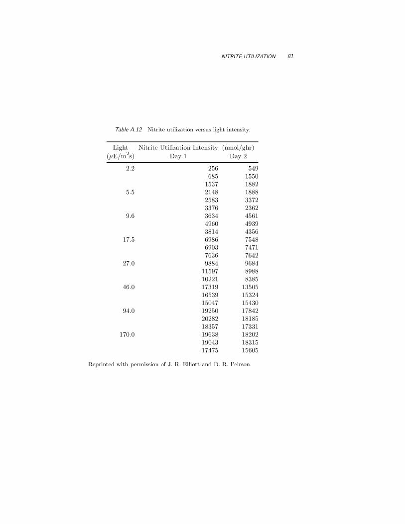
NITRITE UTILIZATION 81
Table A.12 Nitrite utilization versus light intensity.
Light Nitrite Utilization Intensity (nmol/ghr)
(µE/m2s) Day 1 Day 2
2.2 256 549685 1550
1537 18825.5 2148 1888
2583 33723376 2362
9.6 3634 45614960 49393814 4356
17.5 6986 75486903 74717636 7642
27.0 9884 968411597 898810221 8385
46.0 17319 1350516539 1532415047 15430
94.0 19250 1784220282 1818518357 17331
170.0 19638 1820219043 1831517475 15605
Reprinted with permission of J. R. Elliott and D. R. Peirson.
82 DATA SETS USED IN EXAMPLES
andf(x, θ) = θ1(e
−θ3x − e−θ2x)
where f is predicted nitrite utilization and x is light intensity.
A.13 S-PMMA
Data on the dielectric behavior of syndiotactic poly(methylmethacrylate) (s-PMMA) were obtained by Havriliak, Jr. and Negami (1967). A disk of thepolymer was inserted between the two metal electrodes of a dielectric cellwhich formed one arm of a four-armed electrical bridge. The bridge was pow-ered by an oscillating voltage whose frequency f could be changed from 5 to500000 hertz (Hz), and bridge balance was achieved using capacitance andconductance standards. The complex dielectric constant was calculated usingchanges from the standards relative to the cell dielectric constant. Measure-ments were made by simultaneously adjusting the capacitance (real) and theconductance (imaginary) arms of the bridge when it was excited at a specificfrequency. The measured responses were the relative capacitance and relativeconductance (dimensionless). (See Table A.13)
The model is an empirical generalization of two models based on theory.It is written
f(x, θ) = θ2 +θ1 − θ2
[
1 + (i2πxe−θ3)θ4
]θ5
where f is predicted relative complex impedance and x is frequency.
A.14 TETRACYCLINE
Data on the metabolism of tetracycline were presented in Wagner (1967).In this experiment, a tetracycline compound was administered orally to asubject and the concentration of tetracycline hydrochloride in the serum inmicrograms per milliliter (µg/ml) was measured over a period of 16 hours.(See Table A.14)
A 2-compartment model was proposed, and dead time was incorporated as
f(x, θ) = θ3[e−θ1(x−θ4) − e−θ2(x−θ4)]
where f is predicted tetracycline hydrochloride concentration and x is time.
A.15 OIL SHALE
Data on the pyrolysis of oil shale were obtained by Hubbard and Robinson(1950) and are reproduced in Table A.15. Oil shale contains organic matter
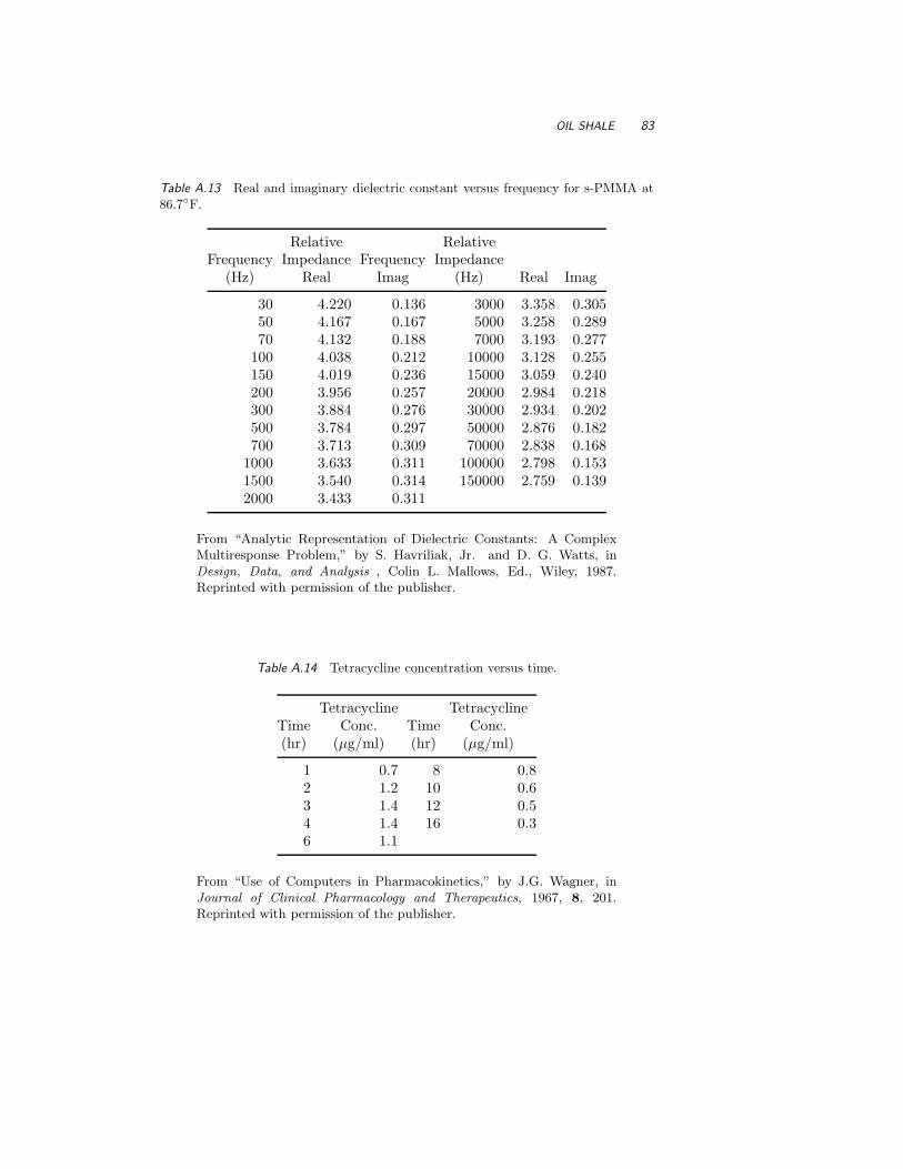
OIL SHALE 83
Table A.13 Real and imaginary dielectric constant versus frequency for s-PMMA at86.7◦F.
Relative RelativeFrequency Impedance Frequency Impedance
(Hz) Real Imag (Hz) Real Imag
30 4.220 0.136 3000 3.358 0.30550 4.167 0.167 5000 3.258 0.28970 4.132 0.188 7000 3.193 0.277
100 4.038 0.212 10000 3.128 0.255150 4.019 0.236 15000 3.059 0.240200 3.956 0.257 20000 2.984 0.218300 3.884 0.276 30000 2.934 0.202500 3.784 0.297 50000 2.876 0.182700 3.713 0.309 70000 2.838 0.168
1000 3.633 0.311 100000 2.798 0.1531500 3.540 0.314 150000 2.759 0.1392000 3.433 0.311
From “Analytic Representation of Dielectric Constants: A ComplexMultiresponse Problem,” by S. Havriliak, Jr. and D. G. Watts, inDesign, Data, and Analysis , Colin L. Mallows, Ed., Wiley, 1987.Reprinted with permission of the publisher.
Table A.14 Tetracycline concentration versus time.
Tetracycline TetracyclineTime Conc. Time Conc.(hr) (µg/ml) (hr) (µg/ml)
1 0.7 8 0.82 1.2 10 0.63 1.4 12 0.54 1.4 16 0.36 1.1
From “Use of Computers in Pharmacokinetics,” by J.G. Wagner, inJournal of Clinical Pharmacology and Therapeutics, 1967, 8, 201.Reprinted with permission of the publisher.

84 DATA SETS USED IN EXAMPLES
Table A.15 Relative concentration of bitumen and oil versus time and temperaturefor pyrolysis of oil shale.
T = 673K T = 698KTime Concentration (%) Time Concentration (%)(min) Bitumen Oil (min) Bitumen Oil
5 0.0 0.0 5.0 6.5 0.07 2.2 0.0 7.0 14.4 1.4
10 11.5 0.7 10.0 18.0 10.815 13.7 7.2 12.5 16.5 14.420 15.1 11.5 15.0 29.5 21.625 17.3 15.8 17.5 23.7 30.230 17.3 20.9 20.0 36.7 33.140 20.1 26.6 25.0 27.3 40.350 20.1 32.4 30.0 16.5 47.560 22.3 38.1 40.0 7.2 55.480 20.9 43.2 50.0 3.6 56.8
100 11.5 49.6 60.0 2.2 59.7120 6.5 51.8150 3.6 54.7
T = 723K T = 748KTime Concentration (%) Time Concentration (%)(min) Bitumen Oil (min) Bitumen Oil
5.0 8.6 0.0 3.0 0.7 0.07.5 15.8 2.9 4.5 17.3 2.98.0 25.9 16.5 5.0 23.0 17.39.0 25.2 24.4 5.5 24.4 20.9
10.0 26.6 29.5 6.0 23.0 25.911.0 33.8 35.2 6.5 33.1 29.512.5 25.9 39.5 7.0 31.6 33.815.0 20.1 45.3 8.0 20.9 45.317.5 12.9 43.1 9.0 10.1 53.217.5 9.3 54.6 10.0 4.3 58.220.0 3.6 59.7 12.5 0.7 57.520.0 2.2 53.9 15.0 0.7 61.1
T = 773K T = 798KTime Concentration (%) Time Concentration (%)(min) Bitumen Oil (min) Bitumen Oil
3.0 6.5 0.0 3.00 25.2 20.94.0 24.4 23.0 3.25 33.1 25.24.5 26.6 32.4 3.50 21.6 17.35.0 25.9 37.4 4.00 20.9 36.75.5 17.3 45.3 5.00 4.3 56.86.0 21.6 45.3 7.00 0.0 61.86.5 1.4 57.5
10.0 0.0 60.4
From “A Thermal Decomposition Study of Colorado Oil Shale,” Hub-bard, A.B. and Robinson, W.E., U.S. Bureau of Mines, Rept. Invest.No. 4744, 1950.
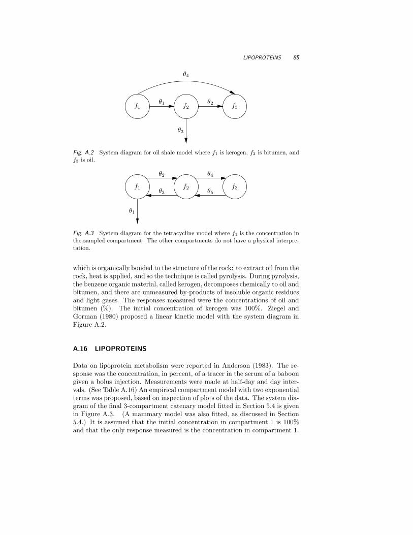
LIPOPROTEINS 85
f1θ1 f2
θ2 f3
θ3
θ4
Fig. A.2 System diagram for oil shale model where f1 is kerogen, f2 is bitumen, andf3 is oil.
f1 f2 f3
θ1
θ2
θ3
θ4
θ5
Fig. A.3 System diagram for the tetracycline model where f1 is the concentration inthe sampled compartment. The other compartments do not have a physical interpre-tation.
which is organically bonded to the structure of the rock: to extract oil from therock, heat is applied, and so the technique is called pyrolysis. During pyrolysis,the benzene organic material, called kerogen, decomposes chemically to oil andbitumen, and there are unmeasured by-products of insoluble organic residuesand light gases. The responses measured were the concentrations of oil andbitumen (%). The initial concentration of kerogen was 100%. Ziegel andGorman (1980) proposed a linear kinetic model with the system diagram inFigure A.2.
A.16 LIPOPROTEINS
Data on lipoprotein metabolism were reported in Anderson (1983). The re-sponse was the concentration, in percent, of a tracer in the serum of a baboongiven a bolus injection. Measurements were made at half-day and day inter-vals. (See Table A.16) An empirical compartment model with two exponentialterms was proposed, based on inspection of plots of the data. The system dia-gram of the final 3-compartment catenary model fitted in Section 5.4 is givenin Figure A.3. (A mammary model was also fitted, as discussed in Section5.4.) It is assumed that the initial concentration in compartment 1 is 100%and that the only response measured is the concentration in compartment 1.

86 DATA SETS USED IN EXAMPLES
Table A.16 Lipoprotein tracer concentration versus time.
Tracer TracerTime Conc. Time Conc.(days) (%) (days) (%)
0.5 46.10 5.0 3.191.0 25.90 6.0 2.401.5 17.00 7.0 1.822.0 12.10 8.0 1.413.0 7.22 9.0 1.004.0 4.51 10.0 0.94
From Compartmental Modeling and Tracer Kinetics, D. H. Anderson, p211, 1983, Springer–Verlag. Reproduced with permission of the authorand the publisher.

References
Anderson, D. H. (1983). Compartmental Modeling and Tracer Kinetics,Springer-Verlag, Berlin.
Ansley, C. F. (1985). Quick proofs of some regression theorems via the QRalgorithm, American Statistician 39: 55–59.
Bache, C. A., Serum, J. W., Youngs, W. D. and Lisk, D. J. (1972). Polychlo-rinated Biphenyl residues: Accumulation in Cayuga Lake trout with age,Science 117: 1192–1193.
Bard, Y. (1974). Nonlinear Parameter Estimation, Academic Press, NewYork.
Bates, D. M. and Watts, D. G. (1981). A relative offset orthogonality conver-gence criterion for nonlinear least squares, Technometrics 23: 179–183.
Belsley, D. A., Kuh, E. and Welsch, R. E. (1980). Regression Diagnostics:
Identifying Influential Data and Sources of Collinearity, Wiley, New York.
Box, G. E. P. (1960). Fitting empirical data, Annals of the New York Academy
of Sciences 86: 792–816.
Box, G. E. P. and Cox, D. R. (1964). An analysis of transformations, Journal
of the Royal Statistical Society, Ser. B 26: 211–252.
Box, G. E. P. and Tiao, G. C. (1973). Bayesian Inference in Statistical Anal-
ysis, Addison-Wesley, Reading, MA.
87

88 REFERENCES
Box, G. E. P. and Tidwell, P. W. (1962). Transformations of the independentvariables, Technometrics 4: 531–550.
Box, G. E. P., Hunter, W. G. and Hunter, J. S. (1978). Statistics for Experi-
menters, Wiley, New York.
Box, G. E. P., Hunter, W. G., MacGregor, J. F. and Erjavec, J. (1973). Someproblems associated with the analysis of multiresponse models, Techno-
metrics 15(1): 33–51.
Carr, N. L. (1960). Kinetics of catalytic isomerization of n-pentane, Industrial
and Engineering Chemistry 52: 391–396.
Chambers, J. M. (1977). Computational Methods for Data Analysis, Wiley,New York.
Chambers, J. M., Cleveland, W. S., Kleiner, B. and Tukey, P. A. (1983).Graphical Methods for Data Analysis, Wadsworth, Belmont, CA.
Cook, R. D. and Weisberg, S. (1982). Residuals and Influence in Regression,Chapman and Hall, London.
Daniel, C. and Wood, F. S. (1980). Fitting Equations to Data: Computer
Analysis of Multifactor Data, 2nd edn, Wiley, New York.
Dongarra, J. J., Bunch, J. R., Moler, C. B. and Stewart, G. W. (1979). Linpack
Users’ Guide, SIAM, Philadelphia.
Draper, N. R. and Smith, H. (1981). Applied Regression Analysis, 2nd edn,Wiley, New York.
Fisher, R. A. (1935). Design of Experiments, Oliver and Boyd, London.
Fuguitt, R. E. and Hawkins, J. E. (1947). Rate of the thermal isomerizationof α-pinene in the liquid phase, J. Amer. Chem. Soc. 69: 319–322.
Hartley, H. O. (1961). The modified Gauss-Newton method for the fitting ofnon-linear regression functions by least squares, Techmometrics 3: 269–280.
Havriliak, Jr., S. and Negami, S. (1967). A complex plane representation ofdielectric and mechanical relaxation processes in some polymers, Polymer
8: 161–205.
Himmelblau, D. M. (1972). A uniform evaluation of unconstrained optimiza-tion techniques, in F. A. Lootsma (ed.), Numerical Methods for Nonlinear
Optimization, Academic Press, London.
Hocking, R. R. (1983). Developments in linear regression methodology: 1959-1982, Technometrics 25: 219–249.

REFERENCES 89
Hougen, O. A. and Watson, K. M. (1947). Chemical Reaction Principles,Wiley, New York.
Hubbard, A. B. and Robinson, W. E. (1950). A thermal decomposition studyof colorado oil shale, Technical Report 4744, U.S. Bureau of Mines.
Jennrich, R. I. and Sampson, P. F. (1968). An application of stepwise regres-sion to non-linear estimation, Techmometrics 10(1): 63–72.
Joiner, B. L. (1981). Lurking variables: Some examples, American Statistician
35: 227–233.
Kaplan, S. A., Weinfeld, R. E., Abruzzo, C. W. and Lewis, M. (1972).Pharmacokinetic profile of sulfisoxazole following intravenous, intramus-cular, and oral administration to man, Journal of Pharmaceutical Sciences
61: 773–778.
Kennedy, Jr., W. J. and Gentle, J. E. (1980). Statistical Computing, MarcelDekker, New York.
Linssen, H. N. (1975). Nonlinearity measures: a case study, Statist. Neerland.
29: 93–99.
Marske, D. (1967). Biochemical oxygen demand data interpretation using sum
of squares surface, PhD thesis, University of Wisconsin–Madison.
Montgomery, D. C. and Peck, E. A. (1982). Introduction to Linear Regression
Analysis, Wiley, New York.
Ralston, M. L. and Jennrich, R. I. (1978). DUD, a derivative-free algorithmfor nonlinear least squares, Technometrics 20: 7–14.
Renwick, A. G. (1982). Pharmacokinetics in toxicology, in A. W. Hayes (ed.),Principles and Methods of Toxicology, Raven Press, New York.
Roller, D. (1950). The Early Development of the Concepts of Temperature and
Heat: The Rise and Decline of the Caloric Theory, Harvard UniversityPress, Cambridge, MA.
SAS (1985). SAS User’s Guide: Statistics, version 5 edn.
Seber, G. A. F. (1977). Linear Regression Analysis, Wiley, New York.
Sredni, J. (1970). Problems of Design, Estimation, and Lack of Fit in Model
Building, PhD thesis, University of Wisconsin–Madison.
Stewart, G. W. (1973). Introduction to Matrix Computations, Academic Press,New York.
Treloar, M. A. (1974). Effects of puromycin on galactosyltransferase of golgi
membranes, Master’s thesis, University of Toronto.

90 REFERENCES
Wagner, J. G. (1967). Use of computers in pharmacokinetics, Clin. Pharma-
cology and Therapeutics 8: 201.
Watts, D. G., deBethizy, D. and Stiratelli, R. G. (1986). Toxicity of ethylacrylate, Technical report, Rohm and Haas Co., Spring House, PA.
Ziegel, E. R. and Gorman, J. W. (1980). Kinetic modelling with multiresponsedata, Technometrics 22: 139–151.