nonlinear models - christian brothers universityfacstaff.cbu.edu/wschrein/media/m105...
TRANSCRIPT
CHAPTER 5
Nonlinear Models
1. Quadratic Function Models
Consider the following table of the number of Americans that are over 100 invarious years.
Year Number (in 1000’s)1994 501996 561998 652000 752002 942004 110
How many would you predict would be over 100 in 2008?
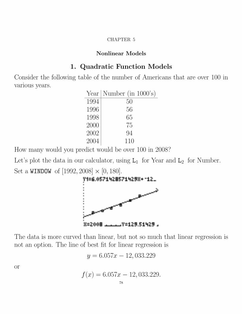
Let’s plot the data in our calculator, using L1 for Year and L2 for Number.
Set a WINDOW of [1992, 2008]⇥ [0, 180].
The data is more curved than linear, but not so much that linear regression isnot an option. The line of best fit for linear regression is
y = 6.057x� 12, 033.229
orf(x) = 6.057x� 12, 033.229.
78

1. QUADRATIC FUNCTION MODELS 79
Add this to the plot as Y1 and look at the graph.
Evaluating f(x) at x = 2008 (2nd/CALC/1:value/X=2008/ENTER) gives
f(2008) = 130.
Visually, this appears to be an underestimation. Recall that regression equa-tions work best with values of x within the boundaries of the data (1994 x 2004). Working outside these boundaries to make predictions is calledextrapolation, and is often not as accurate as working inside the boundaries.Note also that r2 = .96 here, so there is a linear relationship, but how strongthis holds beyond the boundaries of the data is questionable.
What about finding a curve to fit the data? We will try the parabola whichbest fits the data. A parabola is the graph of a quadratic function
y = ax2 + bx + c.
We obtain the quadratic equation of best fit by using quadratic regression(STAT/CALC/5:QuadReg/VARS/Y-VARS/1:Function/1;Y1/ENTER). Note thatr2 = .997 here, so we expect a very good fit:
y = .402x2 � 1600.282x + 1593498.2.
This appears to be a good fit and we expect a good approximation for 2008. Ify = f(x),
f(2008) = 157.

80 5. NONLINEAR MODELS
Parabolas – graphs of y = ax2 + bx + c
a > 0 concave up
a < 0 concave down
|a| = magnitude of a parabola. The greater the magnitude, the steeper theparabola. On the TI:
(1) Compare x2 � 4x + 2 and 4x2 � 4x + 2 on [�3, 6]⇥ [�3, 20].
(2) Compare �x2 � 3x + 5 and �3x2 � 3x + 5 on [�6, 4]⇥ [�10, 10].
Notice that c (or more precisely, (0, c)), is the y-intercept, while b a↵ects thehorizontal and vertical placement of the parabola.
Since the roots of a parabola are the solutions of ax2 + bx + c = 0, they are
x =�b ±
pb2 � 4ac
2a= � b
2a±p
b2 � 4ac
2a
by the quadratic formula, and the x-coordinate of the vertex is x = � b
2a,
which is halfway between the roots. The vertical line x = � b
2ais called the
axis of symmetry.

1. QUADRATIC FUNCTION MODELS 81
The vertex is the point on the graph where the function changes from decreasingto increasing or vice-versa.
Example. Find the concavity, intercepts, and vertex of
f(x) = �2x2 � 2.4x + 14.96
Solution
f is concave down with a magnitude of 2.
The axis of symmetry is
x = � b
2a= � �2.4
2(�2)= �0.6.
Since f(�0.6) = 15.68, the vertex is (�.6, 15.68).
The y-intercept is c = 14.96 = f(0). The x-intercepts are
x =�b ±
pb2 � 4ac
2a= � b
2a±p
b2 � 4ac
2a= �.6 ± (�2.8)
orx = �3.4 and x = 2.2.

82 5. NONLINEAR MODELS
Problem (Page 299 #8).
We are given that the graph is a parabola, so it is the graph of
f(x) = ax2 + bx + c.
Three noncollinear points are su�cient to provide 3 linear equations in a, b, andc that has a unique solution. The graph here appears to pass through (�1, 1),(0, 1), and (1, 3).
From f(0) = c = 1, the y-intercept, we have f(x) = ax2 + bx + 1.
From f(�1) = a� b + 1 = 1, we have a� b = 0.
From f(1) = a + b + 1 = 3, we have a + b = 2.
Adding the last two equations on the right, we have
2a = 2) a = 1) b = 1.
Thus f(x) = x2 + x + 1.Problem (Page 300 #14).
We find the unique quadratic function that fits the three points (0, 6), (20, 68),and (40, 438), the middle point along with the two extremes.
From f(0) = c = 6, the y-intercept, we have f(x) = ax2 + bx + 6.
From f(20) = 400a + 20b + 6 = 68, we have 400a + 20b = 62.
From f(40) = 1600a + 40b + 6 = 438, we have 1600a + 40b = 432.
From the last two equations on the right, we have(�800a� 40b = �124
1600a + 40b = 432
)) 800a = 308) a = .385)
154 + 20b = 62) 20b = �92) b = �4.6.
Thus f(x) = .385x2 � 4.6x + 6.
Note that f(10) = �1.5 6= 16 and f(30) = 214.5 6= 233, so the 2nd and 4thpoints are missed.
1. QUADRATIC FUNCTION MODELS 83
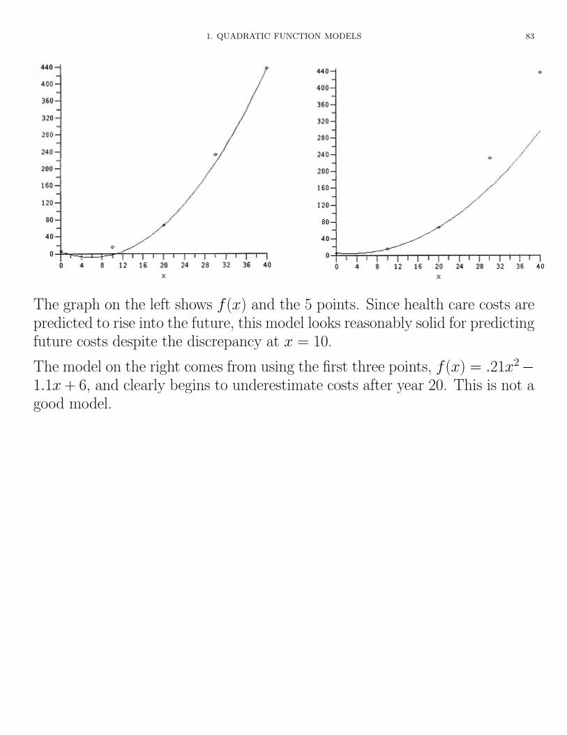
The graph on the left shows f(x) and the 5 points. Since health care costs arepredicted to rise into the future, this model looks reasonably solid for predictingfuture costs despite the discrepancy at x = 10.
The model on the right comes from using the first three points, f(x) = .21x2�1.1x + 6, and clearly begins to underestimate costs after year 20. This is not agood model.
84 5. NONLINEAR MODELS
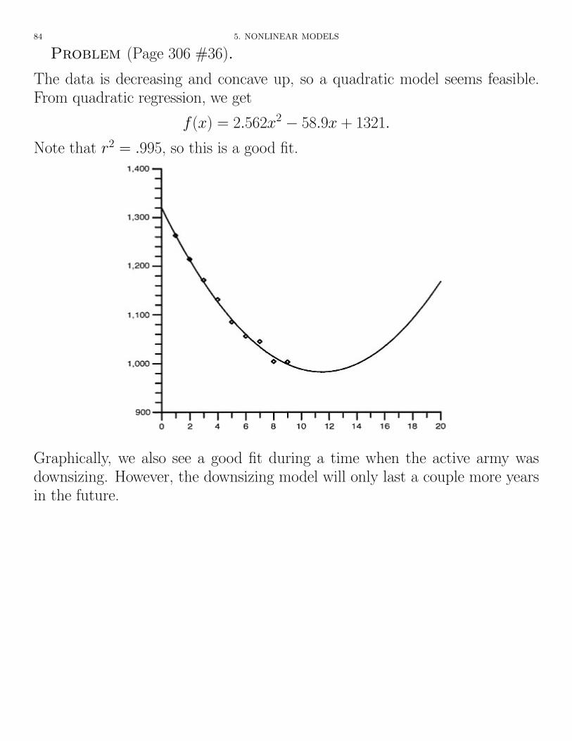
Problem (Page 306 #36).
The data is decreasing and concave up, so a quadratic model seems feasible.From quadratic regression, we get
f(x) = 2.562x2 � 58.9x + 1321.
Note that r2 = .995, so this is a good fit.
Graphically, we also see a good fit during a time when the active army wasdownsizing. However, the downsizing model will only last a couple more yearsin the future.
2. HIGHER POLYNOMIAL FUNCTION MODELS 85
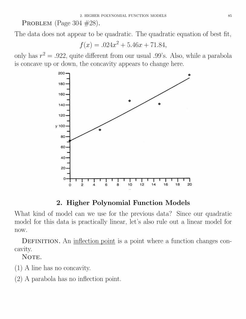
Problem (Page 304 #28).
The data does not appear to be quadratic. The quadratic equation of best fit,
f(x) = .024x2 + 5.46x + 71.84,
only has r2 = .922, quite di↵erent from our usual .99’s. Also, while a parabolais concave up or down, the concavity appears to change here.
2. Higher Polynomial Function Models
What kind of model can we use for the previous data? Since our quadraticmodel for this data is practically linear, let’s also rule out a linear model fornow.
Definition. An inflection point is a point where a function changes con-cavity.
Note.
(1) A line has no concavity.
(2) A parabola has no inflection point.

86 5. NONLINEAR MODELS
Definition. A cubic function is a polynomial of degree 3 and has the form
f(x) = ax3 + bx2 + cx + d.Note.
(1) A cubic function has exactly one inflection point.
(2) If a > 0, we get one of these two shapes (concave down, followed by concaveup).
(3) If a < 0, we get one of these two shapes (concave up, followed by concavedown).
But the data of #28 has two regions of concave up and one of concave downfor 2 inflection points.
Definition. A quartic function is a polynomial of degree 4 and has theform
f(x) = ax4 + bx3 + cx2 + dx + e.
2. HIGHER POLYNOMIAL FUNCTION MODELS 87
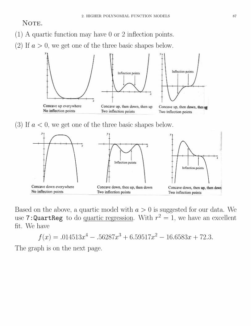
Note.
(1) A quartic function may have 0 or 2 inflection points.
(2) If a > 0, we get one of the three basic shapes below.
(3) If a < 0, we get one of the three basic shapes below.
Based on the above, a quartic model with a > 0 is suggested for our data. Weuse 7:QuartReg to do quartic regression. With r2 = 1, we have an excellentfit. We have
f(x) = .014513x4 � .56287x3 + 6.59517x2 � 16.6583x + 72.3.
The graph is on the next page.
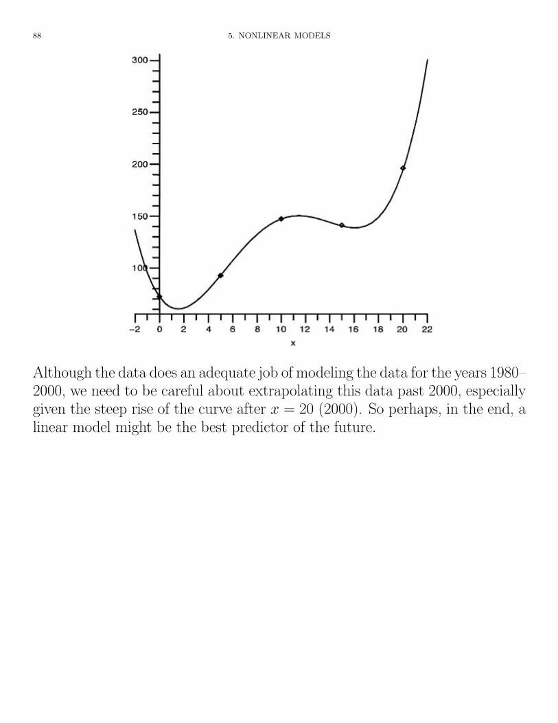
88 5. NONLINEAR MODELS
Although the data does an adequate job of modeling the data for the years 1980–2000, we need to be careful about extrapolating this data past 2000, especiallygiven the steep rise of the curve after x = 20 (2000). So perhaps, in the end, alinear model might be the best predictor of the future.
2. HIGHER POLYNOMIAL FUNCTION MODELS 89
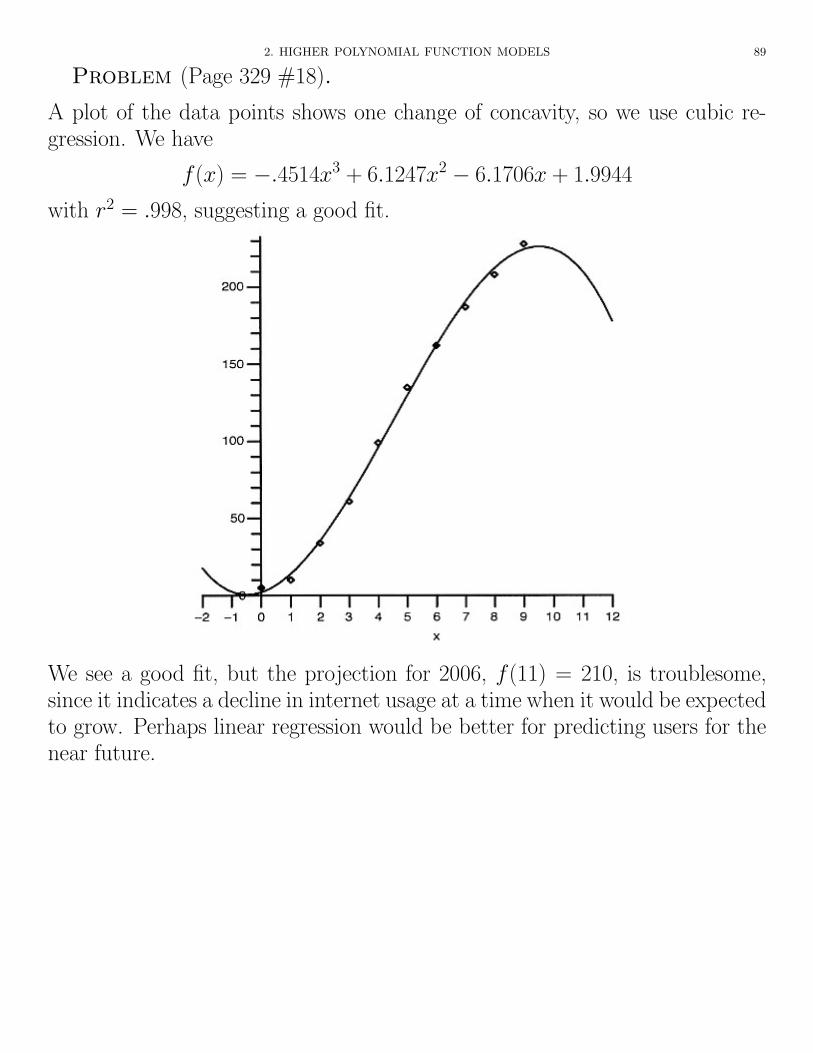
Problem (Page 329 #18).
A plot of the data points shows one change of concavity, so we use cubic re-gression. We have
f(x) = �.4514x3 + 6.1247x2 � 6.1706x + 1.9944
with r2 = .998, suggesting a good fit.
We see a good fit, but the projection for 2006, f(11) = 210, is troublesome,since it indicates a decline in internet usage at a time when it would be expectedto grow. Perhaps linear regression would be better for predicting users for thenear future.

90 5. NONLINEAR MODELS
Problem (Page 324 #4).
The data appears to be linear, but we are asked to use a quadratic, cubic, orquartic model, the simplest to fit the data. Since the data appears slightlyconcave down, we choose the quadratic model. We get
f(x) = �13.9512x2 + 2777.65x + 29155.78
with r2 = .998, suggesting a good fit. Linear regression gives r2 = .997.
This is a model where extrapolation seems plausible over the next period ofyears. It appears salaries will reach $100,000 between years 2010–2011 (x = 30or x = 31).
f(30) = 99, 929
f(31) = 101, 856
3. EXPONENTIAL FUNCTION MODELS 91
3. Exponential Function Models
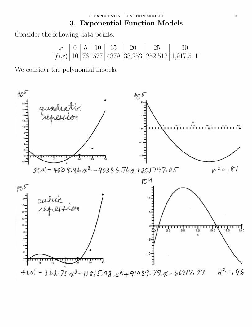
Consider the following data points.
x 0 5 10 15 20 25 30f(x) 10 76 577 4379 33,253 252,512 1,917,511
We consider the polynomial models.

92 5. NONLINEAR MODELS
All of these models have regions of negative values and miss points by 50,000or more, so they are unsatisfactory. Let’s look at something new – exponentialregression.

3. EXPONENTIAL FUNCTION MODELS 93
Clearly, exponential regression gives an almost perfect fit.
Looking back to the data,x 0 5 10 15 20 25 30
f(x) 10 76 577 4379 33,253 252,512 1,917,511we see equal gaps of 5 for x, but not equal gaps for f(x) (as in the linear case).However, consider successive ratios:76
10= 7.6,
577
76= 7.59,
4379
577= 7.59,
33, 253
4379= 7.59,
252, 512
33, 253= 7.59,
1, 917, 511
252, 512= 7.59
We notice a property of exponential functions –
for equal increments of x, the ratio of function values is constant (ignoring somerounding o↵ error).

94 5. NONLINEAR MODELS
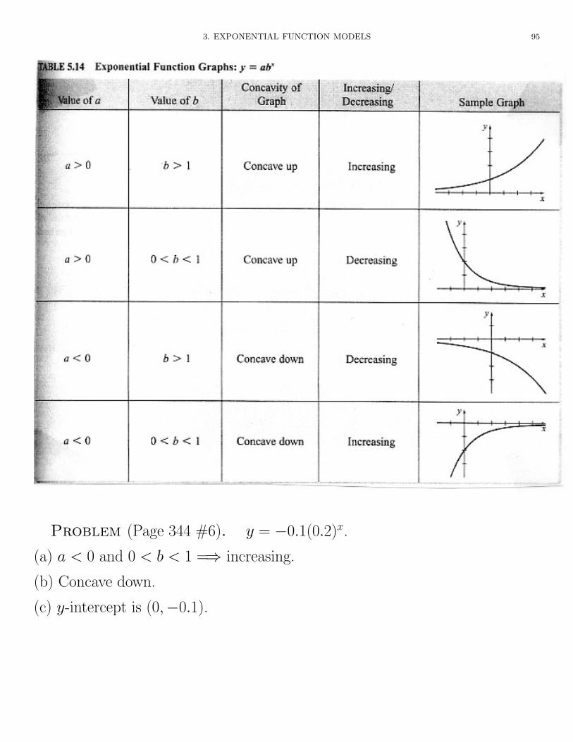
Definition. If a and b are real numbers with a 6= 0, b > 0, and b 6= 1,then the function
y = f(x) = abx
is called an exponential function. The value b is the base of the exponentialfunction.
Note.
(1) Exponential functions are often used to model growth and decay of a quan-tity. In such cases, x (or t, which is more commonly used), represents time,and since
f(0) = ab0 = a · 1 = a,
a is called the initial value of the function.
(2) If a = 0, b = 0, or b = 1, we would have constant functions.
(3) If b < 0, any noninteger powers would be complex or imaginary numbers.
(4) a is the y-intercept of the graph of f(x).
(5) For b > 1, b is called the growth factor.
Example. f(x) = 10(1.5)x.
As x increases by 1, f(x) increases by a factor of 1.5.
f(0) = 10, f(1) = 15 = 1.5(10), f(2) = 22.5 = 1.5(15)
As x increases, the graph moves away from the x-axis.
(6) For 0 < b < 1, b is called a decay factor.
Example. f(x) = 10(12)
x.
As x increases by 1, f(x) decreases by a factor of 12.
f(0) = 10, f(1) = 5 =1
2(10), f(2) = 2.5 =
1
2(5)
As x increases, the graph moves towards the x-axis.
3. EXPONENTIAL FUNCTION MODELS 95
Problem (Page 344 #6). y = �0.1(0.2)x.
(a) a < 0 and 0 < b < 1 =) increasing.
(b) Concave down.
(c) y-intercept is (0,�0.1).

96 5. NONLINEAR MODELS
Problem (Page 344 #18).
Two points with distinct y-coordinates determine a unique exponential function,
y = abx.
To find the two numbers a and b, we need two equations, i.e., two points.
You may use any two points, but write the point with the larger x first.
(5, 32) =) 32 = ab5
(2, 4) =) 4 = ab2
(divide) 8 = b3 =) 81/3 = b =) 2 = b.
Thusy = a · 2x.
(2, 4) =) 4 = a · 22 =) 4 = 4a =) a = 1.
Theny = 1 · 2x.
Problem (Page 344 #20).
y = abx.
(0, 10000) is the y-intercept, so 10000 = ab0 = a · 1 = a. Thus
y = 10000bx.
Now take any other point.
(5, 24.3) =) 24.3 = 10000 · b5 =) b5 =24.3
10000= .00243 =)
b = .002431/5 = .3.
Theny = 10000(.3)x.

3. EXPONENTIAL FUNCTION MODELS 97
Problem (Page 345 #22).
Since t increases by 5’s (evenly), we check successive ratios of I :
100.2
89.5⇡ 1.12,
114.4
100.2⇡ 1.14,
133.6
114.4⇡ 1.17,
151.6
133.6⇡ 1.13.
Since these ratios are approximately the same, exponential regression makessense. We get
I(t) = 88.50876368(1.027197187)t.
For 2005 (t = 25), we haveI(25) = 173.1.
This means that at the end of 2005, the price of wine consumed at home isexpected to be 173.1% of its 1984 price. For example, a bottle of wine costing$20 in 1984 is expected to cost $34.62 in 2005.
Problem (Page 303 #24).
Since the points appear to be concave down, the quadratic model gives us
f(x) = �.052x2 + 3.177x + 34.644
with r2 = .994.

98 5. NONLINEAR MODELS
Even though it fits the data well, it forecasts that the percentage of new homeswith central air will go down, which doesn’t seem likely, so this function is nota good model.
The quartic model also has no inflection points for some cases, so we try thatand get
f(x) = .0000365x4 � .000139x3 � .101x2 + 3.891x + 34
with r2 = 1.
This is an extremly good fit, but would surpass 100% in just a few years, limitingits usefulness.
What kind of curve does the shape of our points suggest? Our data would seemto approach 100 as a horizontal asymptote. The points suggest an exponentialcurve like the bottom curve on page 333. But all those curves have y = 0 as ahorizontal asymptote, not y = 100. So we align the data.
We subtract 100 from each y-value in L2 and put the result in L3. You can dothis easily by putting the cursor on L3 and typing 2nd 2 -100 ENTER. Youthen get the following graph using Plot2 with L1 and L3.

3. EXPONENTIAL FUNCTION MODELS 99
But ExpReg doesn’t work with negative y’s, so we multiply each y in L3 by�1 and put the result in L4. Put the cursor on L4 and type -1 2nd 3 ENTER.Plot3 with L1 and L4 gives a graph like the second one on page 333. ThenExpReg L1, L4, Y1 gives
f(x) = 63.32(.954)x.
Taking its negative and adding 100 (reversing what we did earlier) gives a finalmodel of
f(x) = �63.32(.954)x + 100,
whose graph follows.

100 5. NONLINEAR MODELS
Adjusting Y1 to the final model also gives this graph as Plot1.
Definition. Let y = abt model the amount of a quantity at time t years.The annual growth rate r of the quantity y is given by
r = b� 1.
Similarly, the annual growth factor is
b = r + 1.Note.
(1) r is the decimal form of the percentage.
(2) r > 0 is called appreciation.
(3) r < 0 is called depreciation.

3. EXPONENTIAL FUNCTION MODELS 101
Problem (Page 345 #28).
y = abt
r = �16% = �.16 =) b = �.16 + 1 = .84.
y = a(.84)t
From y(2002) = 599.99, we have
599.99 = a(.84)2002.
But the calculator cannot handle .84 ^ 2002.
So let t = years after 2002.
Then a = 599.99 =)y = 599.99(.84)t.
Since t = 5 for 2007,
y(5) = 599.99(.84)5 = 250.92.
Thus the TV would cost $250.92 in 2007.
Problem (Page 346 #32). Solve (0.9)x = 0.5 graphically.
(1) Graph Y1 = 0.9 ^ x.
(2) Graph Y2 = 0.5.
(3) Set a WINDOW [0, 10]⇥ [0, 2].
(4) Use 2nd/Calc/5:Intersect to get
x = 6.5788.

102 5. NONLINEAR MODELS
4. Logarithmic Function Models
How would we solve an equation like the one in the previous problem,
(0.9)x = 0.5,
algebraically, where the variable is an exponent?
Let’s consider the function y = 3x and the following points on its graph:x 0 1 2 3 4 5y 1 3 9 27 81 243
For what value of x is y = 100, or equivalently, solve
3x = 100.

4. LOGARITHMIC FUNCTION MODELS 103
x is|{z} the exponent we place on| {z } 3|{z} to get 100| {z }.x = log base 3 of 100
Definition. Let b and x be real numbers with b > 0, b 6= 1, and x > 0.The function
y = logb(x) [or y = logb x]
is called a logarithmic function. The value b is called the base of the logarithmicfunction. We read the expression logb(x) as “log base b of x.”
Note. A logarithm is an exponent, and every exponent needs a base.
We view the graph ofx = g(y) = log3 y
along with an illustration of log3 100, which is about 4.2. A partial list of pointsis
y 1 3 9 27 81 243x 0 1 2 3 4 5
Example. Find y = log4 16.
y = 2 since 42 = 16.
Example. Find y = log5 125.
y = 3 since 53 = 125.

104 5. NONLINEAR MODELS
Example. Find y = log3
⇣ 1
81
⌘.
y = �4 since 3�4 =1
34=
1
81.
The most common logarithms are log10, usually just written as log, and loge,usually written as ln for natural logarithm. These have corresponding keys onyour calculator. The number e is generated by letting n!1 in⇣
1 +1
n
⌘nor
⇣n + 1
n
⌘n.
For instance, if n = 1010, we get
2.7 1828|{z} 1828|{z}to 9 decimal places for this irrational number.
Theorem (Change of base formula).
Any logarithm can be written in terms of log and ln by
logbx =log x
log b=
ln x
ln b.

4. LOGARITHMIC FUNCTION MODELS 105
We view the graphs of y = ln x and y = log x together.
All logarithmic graphs pass through the point (1, 0) and have the y-axis as avertical asymptote.
For x > 1, the smaller the base, the larger the values of the logarithm.
For x < 1, the smaller the base, the smaller (more negative) the values of thelogarithm.
When b > 1, logb x increases at a decreasing rate (concave down).
When 0 < b < 1, logb x decreases at an increasing rate (concave up), i.e., at arate that is less and less negative.

106 5. NONLINEAR MODELS
Theorem (Relationship between exponential and logarithmic functions).For b > 0, b 6= 1, and x > 0, the following statements are equivalent:
(1) y = logb x.
(2) by = x.
Consider tables of values for f(x) = 10x and g(x) = log(x).
The output of one function is the input of the other. A point (x, y) is on onegraph if and only if (y, x) is a point on the other graph. Functions with thisproperty are called inverse functions, with each being the inverse of the other.This also means that the line y = x acts as a mirror between the two graphs.

4. LOGARITHMIC FUNCTION MODELS 107
Example. Solve 6x = 216.
With calculator, using inverse relationship:
x = log6 216 =log 216
log 6= 3.
Without calculator:
6x = 216
6x = 63
x = 3
Example. Solve 5x = 1125.
With calculator, using inverse relationship:
x = log51
125=
log 1125
log 5= �3.
Without calculator:
5x =1
125
5x =1
53
5x = 5�3
x = �3
Example. Solve log3(x) = 5.
With or without calculator:
log3(x) = 5
x = 35
x = 243

108 5. NONLINEAR MODELS
Rules of Logarithms
Rule 7 is used extensively in solving exponential equations. Rules 1, 5, 6, 7apply to any base. Rules 2,3,4 can be easily reformulated for any base.
Example. Use rules of logarithms to write as a single logarithm:
(1)
log(3)� log(27) =
log⇣ 3
27
⌘= log
⇣1
9
⌘= log(3�2) =
� 2 log(3)
(2)
4 log(x2)� 5 log(x2) + log(2x3) =
� log(x2) + log(2x3) = log(2x3)� log(x2) =
log⇣2x3
x2
⌘= log(2x)
4. LOGARITHMIC FUNCTION MODELS 109
(3)
3 log⇣ 2
5x
⌘� log(x3) =
log⇣ 2
5x
⌘3� log(x3) = log
⇣ 8
125x3
⌘� log(x3)
log⇣ 8
125x3
x3
⌘= log
⇣ 8
125x6
⌘= 3 log
⇣ 2
5x2
⌘(4)
� ln(3x)2 � 3 ln(x�2)� 5 ln(x) =
� ln(9x2) + 6 ln(x)� 5 ln(x) =
� ln(9x2) + ln(x) = ln(x)� ln(9x2) =
ln⇣ x
9x2
⌘= ln
⇣ 1
9x
⌘=
ln(1)� ln(9x) =
� ln(9x)
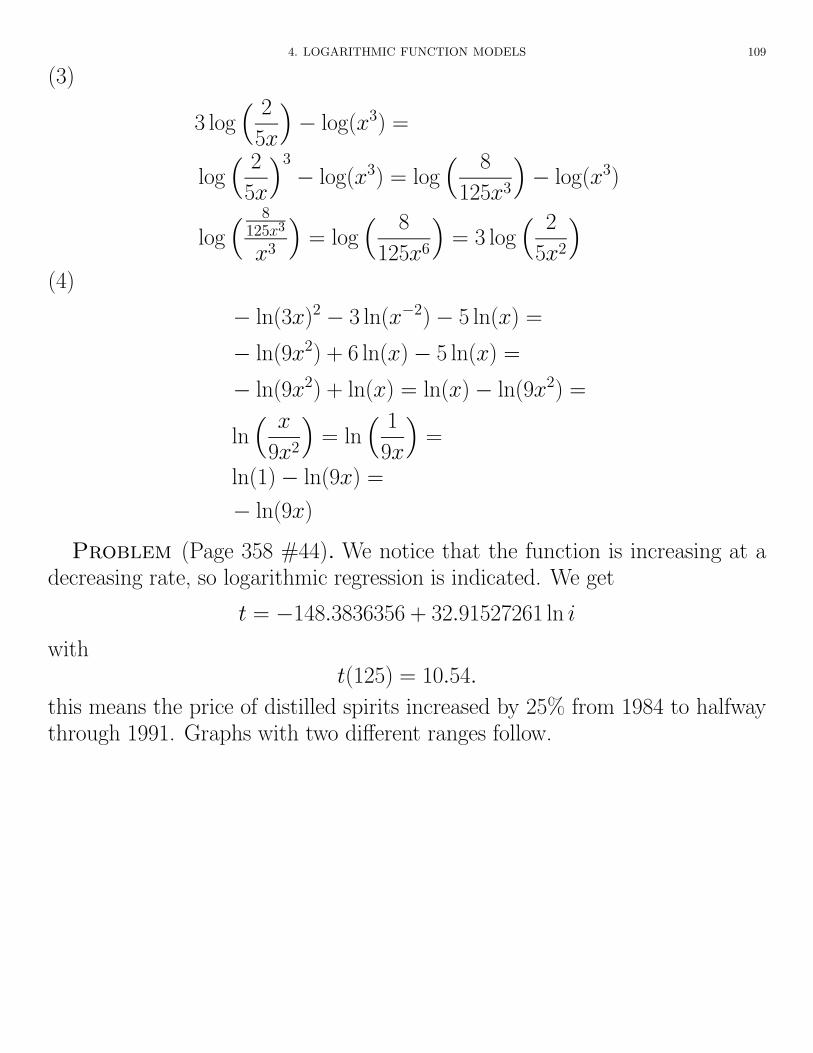
Problem (Page 358 #44). We notice that the function is increasing at adecreasing rate, so logarithmic regression is indicated. We get
t = �148.3836356 + 32.91527261 ln i
witht(125) = 10.54.
this means the price of distilled spirits increased by 25% from 1984 to halfwaythrough 1991. Graphs with two di↵erent ranges follow.

110 5. NONLINEAR MODELS
5. CHOOSING A MATHEMATICAL MODEL 111
5. Choosing a Mathematical Model
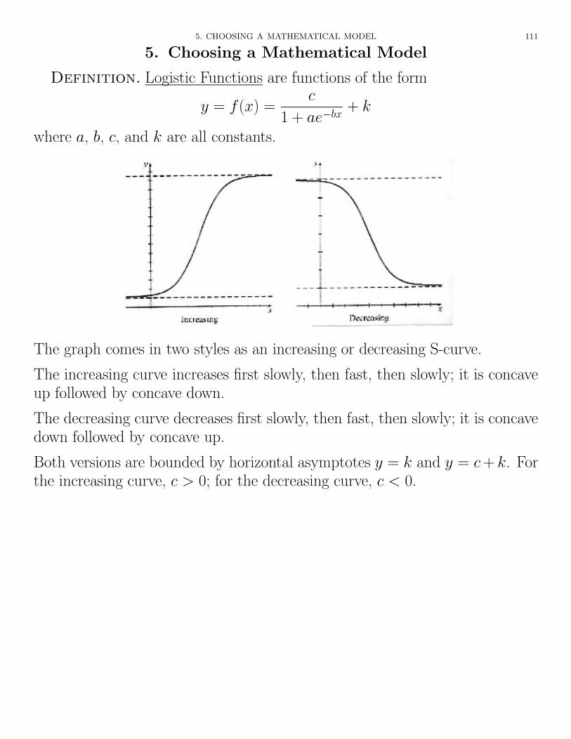
Definition. Logistic Functions are functions of the form
y = f(x) =c
1 + ae�bx+ k
where a, b, c, and k are all constants.
The graph comes in two styles as an increasing or decreasing S-curve.
The increasing curve increases first slowly, then fast, then slowly; it is concaveup followed by concave down.
The decreasing curve decreases first slowly, then fast, then slowly; it is concavedown followed by concave up.
Both versions are bounded by horizontal asymptotes y = k and y = c + k. Forthe increasing curve, c > 0; for the decreasing curve, c < 0.

112 5. NONLINEAR MODELS
Selecting a Mathematical Model.
(1) Draw a scatter plot.
(2) Determine whether the scatter plot exhibits the behavior of the graph ofone or more of the standard mathematical functions: linear, quadratic, cubic,quartic, exponential, logarithmic, or logistic.
(3) Find a mathematical model for each function type selected in step 2.
(4) Use all available information to anticipate the expected behavior of the thingbeing modeled outside of the data set. Eliminate models that don’t exhibit theexpected behavior. (Sometimes it is convenient to switch the order of Steps 3and 4.)
(5) Choose the simplest model from among the models that meet your criteria.
Key features of the various models are given below.

5. CHOOSING A MATHEMATICAL MODEL 113
Problem (Page 371 #6). With the exception of a couple of points, thedata appears to be sort of linear, but a concave up region followed by a concavedown region is evident.
Since tuition is not likely to level o↵, ruling out the logistic model, we look tothe cubic model. We get
f(x) = �.249x3 + 7.447x2 + 9.024x + 634.538.
For 2005, the cubic model gives
f(21) ⇡ 1801,
which seems low. Thus we look to the linear model:
f(x) = 69.612x + 534.076.
For 2005, this givesf(21) ⇡ 1995,
which seems to make more sense based on the data, even though the linearmodel may not fit the points as well.

114 5. NONLINEAR MODELS
Problem (Page 370 #2). The data appears slightly concave up. Candidatemodels are then quadratic and exponential. We check ratios over the last 4points where the x-gaps are equal:
965
987= .978,
946
965= .980,
932
946= .985.
We view the graphs of the models for 30 years (put the quadratic model as Y1
and the exponential as Y2).
For the quadratic model, r2 = .998, while for the exponential, r2 = .977,indicating a better fit for the quadratic model, as is also clear from the graph.Further, the quadratic model matches the leveling o↵ of the loss of farms, whilethe exponential model (whose graph in this window is almost linear) will notlevel o↵ until much closer to the x-axis. So we choose the quadratic model
f(x) = .1249001315x2 � 6.654950848x + 1013.888611.
For the year 2000, this gives us
f(22) ⇡ 928.
This makes sense since we expect the number of farms to continue to decreaseinto the near future.

5. CHOOSING A MATHEMATICAL MODEL 115
116 5. NONLINEAR MODELS
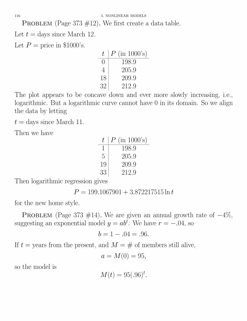
Problem (Page 373 #12). We first create a data table.
Let t = days since March 12.
Let P = price in $1000’s.t P (in 1000’s)0 198.94 205.918 209.932 212.9
The plot appears to be concave down and ever more slowly increasing, i.e.,logarithmic. But a logarithmic curve cannot have 0 in its domain. So we alignthe data by letting
t = days since March 11.
Then we havet P (in 1000’s)1 198.95 205.919 209.933 212.9
Then logarithmic regression gives
P = 199.1067901 + 3.872217515 ln t
for the new home style.
Problem (Page 373 #14). We are given an annual growth rate of �4%,suggesting an exponential model y = abt. We have r = �.04, so
b = 1� .04 = .96.
If t = years from the present, and M = # of members still alive,
a = M(0) = 95,
so the model isM(t) = 95(.96)t.

5. CHOOSING A MATHEMATICAL MODEL 117
Problem (Page 373 #17).
We let x = years since 1990 and y = population. A data table isx y0 266710 431611 494012 5555
Recall logistic regression
y = f(x) =c
1 + ae�bx+ k
has horizontal asymptotes y = k andy = c + k with c > 0 for the increasingcurve and c < 0 for the decreasing curve. However, the TI-83 Plus and TI-84Plus, but not the TI-89, assume that k = 0. For our data, k = 2600 seemsreasonable, so we align the data by making the right hand column y � 2600.
x y � 26000 6710 171611 234012 2955
On the TI, put the cursor on L3, and punch 2nd 2-2600/ENTER to place thealigned data in L3, and then punch STAT/CALC/B:Logistic/2nd 1/,/2nd3/,/Y1/ENTER. We get
y � 2600 =6929.817052
1 + 166.2278249e�.4019008339x
or
y =6929.817052
1 + 166.2278249e�.4019008339x+ 2600.
Since the denominator approaches 1 as x gets large, the model projects a max-imum population of
6930 + 2600 = 9530.

118 5. NONLINEAR MODELS
After adding 2600 to Y1, view the graph in a window [�1, 20]⇥ [0, 10000]. Ourmodel projects a 2003 population of
y(13) = 6258,
quite a bit less than the department of Commerce projection of 7480.
We look for a di↵erent model:
(1) The quadratic and cubic models show population decreases between 1990and 2000, so are rejected. Also, their predictions for 2003 are about the sameas for the logistic model.
(2) We don’t have enough points for the quartic model to work.
(3) We go to the exponential model with the aligned data since we want y = 0as a horizontal asymptote. We use
ExpReg L1, L3, Y1
to gety � 2600 = 67.58587649(1.376627411)x
ory = 67.58587649(1.376627411)x + 2600.
Nowy(13) = 6910,
which is closer to the Department of Commerce projection.Problem (Page 373 #20).
Let x = joint yearly salary and T = taxes owed.
T (x) =
8><>:
.1x if 0 x 14, 000
.1(14, 000) + .15(x� 14, 000) if 14, 000 < x 56, 800
.1(14, 000) + .15(42, 800) + .25(x� 56, 800) if x > 56, 800
.
Then T (x) =
8><>:
.1x if 0 x 14, 000
.15x� 700 if 14, 000 < x 56, 800
.25x� 6380 if 56, 800 < x 114, 650
.