FULL PAPER

Nonlinear GRAPPA: A Kernel Approach to ParallelMRI Reconstruction

Yuchou Chang,1 Dong Liang,1,2 and Leslie Ying1*

GRAPPA linearly combines the undersampled k-space signalsto estimate the missing k-space signals where the coeffi-cients are obtained by fitting to some auto-calibration signals(ACS) sampled with Nyquist rate based on the shift-invariantproperty. At high acceleration factors, GRAPPA reconstructioncan suffer from a high level of noise even with a large numberof auto-calibration signals. In this work, we propose a nonlin-ear method to improve GRAPPA. The method is based on theso-called kernel method which is widely used in machinelearning. Specifically, the undersampled k-space signals aremapped through a nonlinear transform to a high-dimensionalfeature space, and then linearly combined to reconstruct themissing k-space data. The linear combination coefficients arealso obtained through fitting to the ACS data but in the newfeature space. The procedure is equivalent to adding manyvirtual channels in reconstruction. A polynomial kernel withexplicit mapping functions is investigated in this work. Experi-mental results using phantom and in vivo data demonstratethat the proposed nonlinear GRAPPA method can significantlyimprove the reconstruction quality over GRAPPA and itsstate-of-the-art derivatives. Magn Reson Med 000:000–000,2011. VC 2011 Wiley Periodicals, Inc.

Key words: parallel imaging; GRAPPA; nonlinear filtering;reproducible kernel Hilbert space; kernel method; regularization

Among many partially parallel acquisition methods (e.g.,1–9), generalized auto-calibrating partially parallelacquisitions (GRAPPA) (1) has been widely used forreconstruction from reduced acquisitions with multiplereceivers. When the net acceleration factor is high,GRAPPA reconstruction can suffer from aliasing artifactsand noise amplifications. Several methods have beendeveloped in recent years to improve GRAPPA, such aslocalized coil calibration and variable density sampling(10), multicolumn multiline interpolation (11), regulari-zation (12,13), iteratively reweighted least-squares (14),high-pass filtering (15), cross validation (16,17), iterativeoptimization (18), GRAPPA operator (19,20), virtual coilusing conjugate symmetry (21), multislice weighting(22), infinite pulse response filtering (23), cross sampling(24), and filter bank methods (25,26).

The conventional GRAPPA method (1) reconstructs themissing k-space data by a linear combination of theacquired data, where the coefficients for combination areestimated using some auto-calibration signal (ACS) linesusually acquired in the central k-space. Huang et al. (27)analyzed two kinds of errors in GRAPPA reconstruction:truncation error and inversion error. Nana et al. (16,17)extended the analysis and used more general terms:model error and noise-related error. The first kind of errormainly originates from a limited number of ACS lines anddata truncation. When a limited size of k-space signals isobserved or inappropriately chosen instead of the wholek-space, model errors occur in GRAPPA reconstruction.This type of error usually varies with the amount of ACSdata, reduction factor, and the size of the coefficients tobe estimated for reconstruction. For example, a reductionin ACS acquisition usually results in degraded imagequality. Therefore, a large amount of ACS data is neededto reduce this model error but at the cost of prolonged ac-quisition time. The second kind of errors originates fromnoise in the measured data and noise-induced error inestimating the coefficients for linear combination. Regula-rization (12,13) has been used in solving the inverse prob-lem for the coefficients, but significant noise reduction isusually at the cost of increased aliasing artifacts. Iterativereweighted least-squares (14) method reduces the noise-induced error to a greater extent by ignoring noise-induced ‘‘outliers’’ in estimating the coefficients. How-ever, the method is computationally expensive.

In this paper, we focus on the nature of noise-inducederror and develop a novel nonlinear method to reducesuch kind of error. We identify the nonlinear relation-ship between the bias in the estimated GRAPPA coeffi-cients and the noise in the measured ACS data due tothe error-in-variable problem in the calibration step. Thisrelationship suggests that the finite impulse responsemodel currently used in GRAPPA reconstruction is notable to remove the nonlinear noise-induced bias even ifregularization is used. We thereby propose a nonlinearapproach to GRAPPA using the kernel method, namednonlinear GRAPPA. (Note this kernel is a terminology inmachine learning and is different from the GRAPPA ker-nel for linear combination.) The method maps the under-sampled data onto a high dimensional feature spacethrough a nonlinear transform and the data in the newspace are then linearly combined to estimate the missingk-space data. Although the relationship between theacquired and missing k-space data is nonlinear, the rela-tionship can be easily and linearly found in the highdimensional feature space using the ACS data. It isworth noting that the nonlinearity of this approach is

1Department of Electrical Engineering and Computer Science, University ofWisconsin, Milwaukee, Wisconsin 53211, USA.2Paul C. Lauterbur Research Center for Biomedical Imaging, Institute ofBiomedical and Health Engineering, Shenzhen Institutes of AdvancedTechnology, Shenzhen, P. R. China.

*Correspondence to: Leslie Ying, Ph.D., Department of ElectricalEngineering and Computer Science, University of Wisconsin, Milwaukee,Wisconsin 53211. E-mail: leiying@uwm.edu

Received 30 May 2011; revised 4 October 2011; accepted 10 October2011.

DOI 10.1002/mrm.23279Published online in Wiley Online Library (wileyonlinelibrary.com).

Magnetic Resonance in Medicine 000:000–000 (2011)

VC 2011 Wiley Periodicals, Inc. 1

completely different from that in the GRAPPA operatorformulation in Refs. (19,20) where the former is on the k-space data while the latter is on the GRAPPA coeffi-cients through successive application of linear operators.The proposed method not only has the advantage of non-linear methods in representing generalized models thatinclude linear ones as a special case, but also maintainsthe simplicity of linear methods in computation.

THEORY

Review of GRAPPA

In conventional GRAPPA, the central k-space of eachcoil is sampled at the Nyquist rate to obtain ACS data,while the outer k-space is undersampled by some outerreduction factors (ORF). The missing k-space data is esti-mated by a linear combination of the acquired under-sampled data in the neighborhood from all coils, whichcan be represented mathematically as

Sj ky þ rDky ; kx� � ¼XL

l¼1

XB2

t¼B1

XH2

h¼H1

wj;r l; t;hð Þ

�Sl ky þ tRDky ;kx þ hDkx� �

; j ¼ 1; :::; L; r 6¼ tR; ½1�

where Sjðky þ rDky ;kxÞ denotes the unacquired k-spacesignal at the target coil, Sjðky þ tRDky ; kx þ hDkxÞ denotesthe acquired undersampled signal, and wi;jðl; t;hÞdenotes the linear combination coefficients. Here R rep-resents the ORF, l counts all coils, t and h transverse theacquired neighboring k-space data in ky and kx direc-tions, respectively, and the variables kx and ky representthe coordinates along the frequency- and phase-encodingdirections, respectively.

In general, the coefficients depend on the coil sensitiv-ities and are not known a priori. The ACS data are usedto estimate these coefficients. Among all the ACS datafully acquired at the central k-space, each location isassumed to be the ‘‘missing’’ point to be used on the left-hand side of Eq. 1. The neighboring locations with a cer-tain undersampling pattern along the phase encodingdirection are assumed to be the undersampled pointsthat are used on the right-hand side of Eq. 1. This isrepeated for all ACS locations (except boundaries of theACS region) based on the shift-invariant property to fitGRAPPA coefficients to all ACS data. This calibrationprocess can be simplified as a matrix equation

b ¼ Ax; ½2�

where A represents the matrix comprised of the under-sampled points of the ACS, b denotes the vector for the‘‘missing’’ points of the ACS, and x represents the coeffi-cients to be fitted. ThematrixA is of sizeM� KwithM beingthe total number of ACS data (excluding the boundaries) andK being the number of points in the neighborhood from allcoils that are used in reconstruction. The least-squaresmethod is commonly used to calculate the coefficients:

x ¼ minx

b�Axk k2: ½3�

When the matrix A is ill-conditioned, the noise can begreatly amplified in the estimated coefficients. To

address the ill-conditioning issue, regularization meth-ods (12,13) have been used to solve for coefficients usinga penalized least-squares method,

x ¼ minx

b�Axk k2þlRðxÞ; ½4�

where R(x) is a regularization function (e.g., R(x) ¼||x||2 in Tikhonov) and l is regularization parameter.Regularization can effectively suppress noise to a certainlevel. However, aliasing artifacts usually appear inreconstruction at the same time while large noise issuppressed.

Another source of noise-induced error in GRAPPA is‘‘outliers.’’ Outliers are k-space data with large measure-ment errors due to noise and low sensitivity. They leadto large deviations in the estimated coefficients from thetrue ones when the least squares fitting is used. Iterativereweighted least-squares method (14) has been proposedto minimize the effect of outliers in least-squares fitting.The method iteratively assigns and adjusts weights forthe acquired undersampled data. ‘‘Outliers’’ are givenless weights or removed in the final estimation, so thatthe fitting accuracy and reconstruction quality areimproved. However, the high computational complexityof the method limits its usefulness in practice.

Errors-in-Variables Model of GRAPPA

The conventional GRAPPA formulation in Eqs. 1 or 2models the calibration and reconstruction as a standardlinear regression and prediction problem, where theundersampled part of the ACS corresponds to the regres-sors and the rest is the regressands. With this formula-tion, if the undersampled points of the ACS (regressors)are measured exactly or observed without noise, andnoise is present only in the ‘‘missing’’ ones of the ACS(regressands), then the least-squares solution is optimaland the error in the reconstruction is proportional to theinput noise. However, this is not the case in GRAPPAbecause all ACS data are obtained from measurementand thus contain the same level of noise.

To understand the effect of noise in both parts of theACS data (regressors and regressands), we describe theregression and prediction process of GRAPPA usinglatent variables (28). Specifically, if A and b are observedvariables that come from the ACS data with measure-ment noise, we assume that there exist some unobservedlatent variables A and b representing the true, noise-freecounterparts, whose true functional relationship is mod-eled as a linear function f. We thereby have

A ¼ ~Aþ dAb ¼ ~bþ dbf : ~b ¼ ~A~x

8<: ½5�

where dA and db represent measurement noises that arepresent in the ACS data and assumed to be independentof the true value A and b, and x denotes the latent truecoefficients for the linear relationship between A and bwithout the hidden noise.

In the standard regression process, the coefficients x isestimated by fitting to the observed data in A and b:

2 Chang et al.

b ¼ Ax ! ~bþ db ¼ ~Aþ dA� �

x: ½6�

Therefore, there is a bias dx ¼ x-x in the coefficientsestimated from the least-squares fitting, where

x ¼ ½ ~Aþ dA� �T ~Aþ dA

� ���1 ~Aþ dA� �Tð~bþ dbÞ: ½7�

For example, consider the simplest case where x is ascalar and b and A are both column vectors whose ele-ments bt and at represent measurements at index t. Theestimated coefficient is given by

x ¼XTt¼1

atbt

,XTt¼1

a2t ; ½8�

which deviates from the true coefficient x ¼ b/a. Whenthe number of measurements T increases without bound,the estimated coefficient converges to

x ¼ ~x�ð1þ s2

b=s2AÞ; ½9�

where the noise in A and b is assumed to have zeromean and variance of s2

A and s2b, respectively. It suggests

that even if there are an infinite number of measure-ments, there is still a bias in the least-squares estimator.Since the bias depends on the noise in both A and b, itseffects on the estimated coefficients x are also noise-like.In the multivariable case, the bias of GRAPPA coeffi-cients is not easily characterized analytically, but isknown to be upper bounded by (Theorem 2.3.8 in Ref.(29))

jjdx jj2jjxjj2

� kð~AÞ jjdAjjjj~Ajj þ

jjdbjjjjbjj þ

jjdAjjjj~Ajj

jjdbjjjjbjj

!; ½10�

where k(A) is the condition number of matrix A. Thebound in Eq. 10 suggests that the bias in GRAPPA coeffi-cients can be large at high reduction factors due to ill-conditioned A (12). In addition, the bias is not a linearfunction of the noise in the ACS. This is known as theerrors-in-variable problem in regression. Figure 1 uses anexample to demonstrate the nonlinearity of the bias forGRAPPA coefficients as a function of noise in the ACSdata. Specifically, a set of brain data with simulated coilsensitivities (obtained from http://www.nmr.mgh.harvar-d.edu/�fhlin/) was used as the noise-free signal. We cal-culated the bias for GRAPPA coefficients (with thecoefficients obtained from the noise-free signal as refer-ence) when different levels of noise were added on all24 lines of the ACS data. We plotted the normalized biasfor GRAPPA coefficients as a function of the normalizednoise level added to the ACS data. It is seen that the biasis not a linear function of noise level. However, whenthe noise is sufficiently low, the curve is well approxi-mated by a straight line and the bias–noise relationshipis approximately linear. Total least squares (30,31) is alinear method used to alleviate the problem by solvingEq. 6 using the total least squares instead of leastsquares. It addressed the error-in-variable problem tosome extent when the noise is low. In the reconstruction

step of GRAPPA, when the biased coefficients x areapplied upon the noisy undersampled data A to estimatethe missing data in outer k-space, errors presented in thereconstruction are given by

y� ~A~x ¼ ~Aþ dA� �ð~xþ dxÞ � ~A~x ¼ ~Adx þ ~xdA þ dAdx ½11�

It shows the effect of biased coefficients on the esti-mated missing k-space data is also nonlinear and noise-like. A comprehensive statistical analysis of noise inGRAPPA reconstruction can be found in (32).

Proposed Nonlinear GRAPPA

All existing GRAPPA derivatives are based on the linearmodel in Eq. 1 without considering the nonlinear biasdue to noise in the ACS data. To address the nonlinear,noise-like errors in GRAPPA reconstruction, a kernelmethod is proposed to describe the nonlinear relation-ship between the acquired undersampled data and themissing data in the presence of noise-induced errors.Please note that the kernel used in this paper is differentfrom the kernel usually used in GRAPPA literature torepresent the k-space neighborhood for linearcombination.

General Formulation Using Kernel Method

Kernel method (33–36) is an approach that is widelyused in machine learning. It allows nonlinear algorithmsthrough simple modifications from linear ones. The ideaof kernel method is to transform the data nonlinearly toa higher dimensional space such that linear operationsin the new space can represent a class of nonlinear oper-ations in the original space. Specifically, given a linearalgorithm, we map the data in the input space A to thefeature space H via a nonlinear mapping F(�): A!H, andthen run the algorithm on the vector representation F(a)of the data. However, the map may be of very high oreven infinite dimensions and may also be hard to find.In this case, the kernel becomes useful to perform the

FIG. 1. Nonlinearity of the bias for GRAPPA coefficients as a

function of noise in ACS data.

Nonlinear GRAPPA 3

algorithms without explicitly computing F(�). More pre-cisely, a kernel is related to the mapping F in that

k a1;a2ð Þ ¼< F a1ð Þ;F a2ð Þ >; 8a1; a2 2 A; ½12�

where <,> represents the inner product. Many differenttypes of kernels are known (36) and the most generalused ones include polynomial kernel (37) and Gaussiankernel (38).

To introduce nonlinearity into GRAPPA, we apply anonlinear mapping to the undersampled k-space data ai ¼{Slðky þ tRDky ; kx þ hDkxÞ} in the neighborhood of eachmissing point where l counts all coils and t and h trans-verse the acquired neighboring k-space data in ky and kxdirections, respectively. Under such a mapping, Eq. 2 istransformed to the following new linear system of x:

b ¼ FðAÞx; ½13�

where F(A) ¼ [F(a1), F(a1), . . ., F(aM)]T, with ai being the

ith row vector of the matrix A defined in Eq. 2. The newmatrix F(A) is of M � NK, where NK is the dimension inthe new feature space which is usually much higher thanK. Equation 13 means the missing data in b is a linear com-bination of the new data in feature space which are gener-ated from the original undersampled k-space data A.

Although Eq. 13 is still a linear equation of the coefficientsx, it mathematically describes the nonlinear relationshipbetween the undersampled and missing data because ofthe nonlinear mapping function F(�). With the ACS data,the regression process to find the coefficients x in Eq. 13for the proposed nonlinear GRAPPA can still be solved bya linear, least-squares algorithm in feature space

x ¼ FH Að ÞF Að Þ� ��1FH Að Þb: ½14�

Once the coefficients are estimated in Eq. 14, they areplugged back in Eq. 13 for the prediction process toreconstruct the missing data in outer k-space, like the

FIG. 2. Illustration of the calibration procedure for GRAPPA andnonlinear GRAPPA.

FIG. 3. Phantom images recon-structed from an eight-channeldataset with an ORF of 6 and 38

ACS lines (denoted as 6–38 onthe right corner of each image).

With the sum of squares recon-struction as the reference, theproposed nonlinear GRAPPA

method is compared with conven-tional GRAPPA, regularized

GRAPPA, and IRLS methods. Thecorresponding difference imageswith the reference (7� amplifica-

tion) and g-factor maps are alsoshown on the right two columns,

respectively.

4 Chang et al.

conventional GRAPPA does. Figure 2 summarizes theabove procedure and illustrates the nonlinear and linearparts of the proposed method (NL GRAPPA) in compari-son to the conventional GRAPPA. It can be seen that theproposed method introduces an additional nonlinearmapping step into GRAPPA to pre-process the acquiredundersampled data while the computational algorithm tofind the coefficients is still the linear least-squaresmethod. Other linear computational algorithms such asreweighted least-squares and total least-squares methodscan also be used here.

Choice of Nonlinear Mapping F(�)To choose the optimal kernel or feature space is not triv-ial. For example, Gaussian kernel has been proved to beuniversal, which means that linear combinations of thekernel can approximate any continuous function. How-ever, overfitting of the calibration data may arise as aresult of this powerful representation. Given the successof GRAPPA, we want the nonlinear mapping to be asmooth function that includes the linear one as a specialcase when the dimension of the feature space is as lowas the original space. Since polynomials satisfy thedesired properties, we choose an inhomogeneous poly-nomial kernel of the following form

k ai; aj� � ¼ gaTi aj þ r

� �d; ½15�

where g and r are scalars and d is the degree of the poly-nomial. Another advantage of polynomial kernel lies inthe fact that its corresponding nonlinear mapping F(a)such that kða1; a2Þ ¼< Fða1Þ;Fða2Þ > has explicit repre-sentations. For example, if c ¼ r ¼ 1 and d ¼ 2, U(a) isgiven by (39)

F að Þ ¼ 1;ffiffiffi2

pa1; . . . ;

ffiffiffi2

paK ; a

21; . . . ;a

2K ;

ffiffiffi2

pa1a2; . . . ;

hffiffiffi2

paiaj ; . . . ;

ffiffiffi2

paK�1aK �T ; ½16�

where a1, a2, . . ., aK are components of the vector a andthere are (Kþ2)(Kþ1)/2 terms in total. It is seen that thevector includes the linear terms in the original space aswell as the constant and second-order terms.

When all possible terms in F(a) are included, directuse of the kernel function may be preferred over the useof nonlinear mapping in Eq. 13 for the sake of computa-tional complexity. However, our experiment (see Fig. 8)shows that the reconstruction using kernel functions suf-fers from blurring and aliasing artifacts. This is becausethe model is excessively complex and represents a toobroad class of functions, and thus the model has been

FIG. 4. Axial brain images recon-structed from a set of eight-chan-nel data with an ORF of 5 and 48

ACS lines using GRAPPA, regular-ized GRAPPA, IRLS, and the pro-

posed nonlinear method. Thecorresponding difference imageswith the reference (5� amplifica-

tion) are shown on the middle col-umn and g-factor maps on theright column.

Nonlinear GRAPPA 5

overfit during calibration but poorly represents the miss-ing data. This overfitting problem can be addressed byreducing the dimension of the feature space (40). Thereduction of feature space is achieved here by keepingthe constant term and all first-order termsffiffiffi2

pa1; . . . ;

ffiffiffi2

pak , but truncating the second-order terms in

vector U(a). Specifically, we sort the second-order termsaccording to the following order. We first have thesquare terms within each coil, and then the productterms between the nearest neighbors, the next-nearestneighbors, and so on so forth in k-space. The above orderis then repeated for terms that are across different coils.With the sorted terms, we can truncate the vector U(a)according to the desired dimension of the feature space.

The performance of the proposed method depends onthe number of second-order terms. If the number is toolow, prediction is inaccurate because the feature space is

not complex enough to accurately describe the true rela-tionship between the calibration and undersampled datain presence of noise, and thus the reconstruction resem-bles GRAPPA and still suffers from noise-like errors. Onthe other hand, if the dimension is too high, the modelis overfit by the calibration data but poorly representsthe missing data, thus leading to aliasing artifacts andloss of resolution in reconstruction. This is known as thebias–variance tradeoff and is demonstrated using anexample in Results section.

Explicit Implementation of Nonlinear GRAPPA

We find heuristically (elaborated in Results section) thatit is sufficient to keep the number of the second-orderterms to be about three times that of the first-order terms.That is, the feature space is reduced to

~F að Þ ¼ ½1;ffiffiffi2

pa1;

ffiffiffi2

pa2; � � � ;

ffiffiffi2

paK ;a

21; a

22; � � � ;a2K|fflfflfflfflfflfflfflfflfflffl{zfflfflfflfflfflfflfflfflfflffl}K

;a1a2; � � � ;aiaj ; � � � ;aK�1aK|fflfflfflfflfflfflfflfflfflfflfflfflfflfflfflfflfflfflfflfflfflfflffl{zfflfflfflfflfflfflfflfflfflfflfflfflfflfflfflfflfflfflfflfflfflfflffl}�K

;a1a3; � � � ; apaq; � � � ;aK�2aK|fflfflfflfflfflfflfflfflfflfflfflfflfflfflfflfflfflfflfflfflfflfflfflffl{zfflfflfflfflfflfflfflfflfflfflfflfflfflfflfflfflfflfflfflfflfflfflfflffl}�K

�; ½17�

where (ai, aj) are nearest neighbors and (ap, aq) arenext-nearest neighbors in k-space along kx within eachcoil. We also find that a slight increase in the number ofsecond-order terms does not change the reconstructionquality, but increases the computation.

After plugging the above truncated mapping vector~FðaÞ in Eq. 17 into the matrix representation in Eq. 13and changing to the notations in conventional GRAPPA,the proposed nonlinear GRAPPA method is thereby for-mulated as

Sjðky þ rDky ;kxÞ ¼ wð0Þj;r � 1þ

XLl¼1

XB2

b¼B1

XH2

h¼H1

wð1Þj;r ðl; b;hÞ � Slðky þ bRDky ;kx þ hDkxÞ

þXLl¼1

XB2

b¼B1

XH2

h¼H1

wð2;0Þj;r ðl;b;hÞ � S2

l ðky þ bRDky ;kx þ hDkxÞ

þXLl¼1

XB2

b¼B1

XH2�1

h¼H1

wð2;1Þj;r ðl;b;hÞ � Slðky þ bRDky ;kx þ hDkxÞ � Slðky þ bRDky ; kx þ ðhþ 1ÞDkxÞ

þXLl¼1

XB2

b¼B1

XH2�2

h¼H1

wð2;2Þj;r ðl;b;hÞ � Slðky þ bRDky ;kx þ hDkxÞ � Slðky þ bRDky ; kx þ ðhþ 2ÞDkxÞ; ½18�

where the same notations are used as in Eq. 1.

The above nonlinear formulation represents a more

general model for GRAPPA, which includes the conven-

tional GRAPPA as a special case. It is seen that the

first-order term of nonlinear GRAPPA in Eq. 18 is

equivalent to the conventional GRAPPA, which mainly

captures the linear relationship between the missing

and acquired undersampled data in the absence of noise

and approximations. The second-order terms of Eq. 18

can be used to characterize other nonlinear effects in

practice such that noise and approximation errors are

suppressed in reconstruction. The proposed formulation

is a nonlinear model in the sense that nonlinear combi-

nation of acquired data contributes to estimation of

missing k-space data. However the computational algo-

rithm is still linear because the new system equation in

Eq. 13 is still a linear function of the unknown coeffi-

cients and can still be solved by the linear least-squares

method.

To better interpret the nonlinear GRAPPA method, we

can consider the nonlinear terms as additional virtual

channels as done in Ref. (21). For example, the first-

order term in Eq. 18 represent a linear combination of L

physical channels, while each second-order term repre-

sents a set of additional L virtual channels. Therefore,

there are 4L channels in total when Eq. 18 is used. More

second-order terms provide more virtual channels. It is

worth noting that different from the true physical chan-

nel, there is no equivalent concept of coil sensitivities

for the virtual channels. This is because the additional

virtual channels are nonlinear function of the original

physical channels. For example, the ‘‘square channel’’

takes the square of the k-space data point-by-point. In

image domain, this is equivalent to the sensitivity-modu-

lated image convolves with itself. Therefore, the result-

ing image cannot be represented as the product of the

original image and another independent ‘‘sensitivity’’

function. Another point to be noted is that the virtual

6 Chang et al.

channels are not necessarily all independent. Only add-

ing channels that are linearly independent can improve

the reconstruction performance. Choosing independent

channels needs further study in our future work.

MATERIALS AND METHODS

The performance of the proposed method was validatedusing four scanned datasets. The first three scanneddatasets were all acquired on a GE 3T scanner (GEHealthcare, Waukesha, WI) with an 8-channel head coil,and the last one was acquired on a Siemens 3T scanner(Siemens Trio, Erlangen, Germany). In the first dataset, auniform water phantom was scanned using a gradientecho sequence (TE/TR ¼ 10/100 ms, 31.25 kHz band-width, matrix size ¼ 256 � 256, FOV ¼ 250 mm2). Thesecond dataset was an axial brain image acquired using a2D spin echo sequence (TE/TR ¼ 11/700 ms, matrix size¼ 256 � 256, FOV ¼ 220 mm2). The third one was a sag-ittal brain dataset acquired using a 2D spin echosequence (TR ¼ 500 ms, TE ¼ min full, matrix size ¼256 � 256, FOV ¼ 240 mm2). In the fourth dataset, car-diac images were acquired using a 2D trueFISP sequence(TE/TR¼1.87/29.9 ms, bandwidth 930 Hz/pixel, 50degree flip angle, 6mm slice thickness, 34 cm FOV inreadout direction, 256 � 216 acquisition matrix) with a4-channel cardiac coil. Informed consents were obtained

for all in vivo experiments in accordance with the insti-tutional review board policy.

The proposed method was compared with conventionalGRAPPA, as well as two existing methods that improve theSNR, Tikhonov regularization (12), and iterativereweighted least squares (IRLS) (14). The root sum ofsquares reconstruction from the fully sampled data of allchannels was shown as the reference image for comparison.The size of the coefficients (blocks by columns) was chosenoptimally for each individual method by comparing themean-squared errors resulting from different sizes. The g-factor map was calculated using Monte Carlo simulationsas described in (41) and used to show noise amplification.It is worth noting that for nonlinear algorithms, the SNRloss depends on the input noise level, and the g-factorsshown in Results section are valid only in a small rangearound the noise level used in this study. Difference imageswere used to show all sources of errors, including blurring,aliasing, and noise. All methods were implemented inMATLAB (Mathworks, Natick, MA). To facilitate visualcomparison, difference images from the reference andzoomed-in patches were also shown for some reconstruc-tions. A software implementation of the proposed nonlin-ear GRAPPA method is available at https://pantherfile.uwm.edu/leiying/www/index_files/software.htm.

RESULTS

Phantom

Figure 3 shows the reconstructions of the phantom usingsum of squares, GRAPPA, Tikhonov regularization, IRLS,and the proposed nonlinear GRAPPA for an ORF of 6and the ACS of 38 (net acceleration of 3.41). The size ofthe coefficients was chosen optimally for each individualmethod, though the image quality is not sensitive to thechange of size within a large range of the optimal choice.The size of the coefficients for nonlinear GRAPPA wastwo blocks and 15 columns and that for the other meth-ods was four blocks and nine columns. It is seen that theconventional GRAPPA suffers from serious noise. Tikho-nov regularization and IRLS can both improve the SNRto some extent but at the cost of aliasing artifacts. Theproposed nonlinear GRAPPA method suppresses most ofthe noise without additional artifacts or loss of resolu-tion. In addition, difference images with the referenceand g-factor maps shown in Fig. 3 also suggest that thenoise-like errors have quite different distributions spa-tially and they are more uniformly distributed in nonlin-ear GRAPPA than in other methods.

In Vivo Brain Imaging

Figures 4 and 5 show the reconstruction results for thetwo in vivo brain datasets, axial and sagittal, respec-tively. An ORF of 5 and the ACS of 48 were used with anet acceleration of 2.81. Nonlinear GRAPPA used a sizeof two blocks and 15 columns, while the other methodsused that of four blocks and nine columns. The differ-ence images with the reference are also shown (amplifiedfive and nine times for display) in both Figs. 4 and 5and g-factor maps are shown for the axial dataset in Fig.4. It is seen that the reconstruction using the proposed

FIG. 5. Sagittal brain images reconstructed from a set of eight-channel data with an ORF 5 and 48 ACS lines and their corre-

sponding difference images on the right. The proposed nonlinearGRAPPA suppresses most noise without aliasing artifacts.

Nonlinear GRAPPA 7

method achieves a quality superior to all other methods.The proposed method effectively removes the spatiallyvarying noise in the conventional GRAPPA reconstruc-tion without introducing aliasing artifacts as Tikhonovregularization and IRLS methods do. Furthermore, theproposed method also preserves the resolution of theaxial image without blurring. There is only a slight lossof details in the sagittal image due to the tradeoffbetween noise suppression and resolution preservation(discussed later in Fig. 8).

In Vivo Cardiac Imaging

Figure 6 shows the results for the in vivo cardiac datasetin long axis. The ORF is 5 and number of ACS lines is

48 (net acceleration of 2.60). The size of the nonlinearGRAPPA coefficients was four blocks and 15 columns.The other methods used a size of four blocks and threecolumns. The ventricle areas are zoomed to show moredetails. Both the difference images and the g-factor mapsare shown for all methods. The same conclusion can bemade that the nonlinear GRAPPA method can signifi-cantly suppress the noise in GRAPPA and still preservethe resolution and avoid artifacts.

We also used the cardiac dataset to study how thenumber of second-order terms affects the nonlinearGRAPPA reconstruction quality. Specifically, we trun-cate all the sorted second-order terms to keep the num-ber to be N times (e.g., three times in Eq. 18) that of thefirst-order terms. The normalized mean squared errors

FIG. 6. Results from the four-channel cardiac dataset with an ORF 5 and 48 ACS lines. The reconstructed images, zoomed ROI, differ-

ence images, and g-factor maps are shown from left to right, respectively. They show that the proposed method can remove morenoise than other methods while still preserving the resolution.

8 Chang et al.

(NMSE) was calculated and plotted as the function ofthe number of the first-order terms in Fig. 7. In consider-ation of computational complexity, only the central 64columns of the 48 ACS lines were used here for calibra-tion. The two endpoints of the curve are the extremecases of the proposed method. The left one correspondsto conventional GRAPPA without the second-orderterms, and the right one is the case where all second-order terms are included (implemented efficiently using

kernel representation directly). Figure 8 shows the corre-sponding reconstructions at some points of the curve.Both the curve and the images suggest that too small ortoo large N deteriorates reconstruction quality. When thenumber N increases, noise is gradually suppressed, butthe resolution gradually degrades and aliasing artifactsgradually appear due to the overfitting problem. Theoptimal range for the value of N to balance the tradeoffbetween noise, resolution, and aliasing artifacts is seento be 3-4 times of the number of the first-order terms,according to both the normalized mean squared errorcurve and the images. Because the value of N directlyaffects the computational complexity, N ¼ 3 was chosenand shown to work well for all datasets tested in thisstudy.

DISCUSSION

We have shown in Results section that the proposednonlinear GRAPPA method can outperform GRAPPA athigh ORFs but also with a large number of ACS lines. Itis interesting to see how the method behaves at lowerORFs or with fewer ACS lines. In Fig. 9, we compareGRAPPA and nonlinear GRAPPA with decreasing ORFswhen the number of ACS lines is fixed to be 40. At alow ORF of 2, both methods perform similarly well. Theproposed method has a slightly lower level of noise. AsORF increases, GRAPPA reconstruction begins to deteri-orate due to the increased level of noise. In contrast, the

FIG. 9. Comparison between GRAPPA and nonlinear GRAPPA

when ORF increases with fixed ACS lines. Contrary to GRAPPA,noise in the proposed method does not increase with the ORF.

FIG. 7. Normalized mean squared error curves of the proposedmethod as a function of the number of the second-order terms

using the long-axis cardiac dataset. The ‘‘U’’ shape of the curvesuggests that some intermediate number should be chosen.

FIG. 8. The nonlinear GRAPPA reconstructions with an increasingnumber of the second-order terms show that the noise is gradu-ally removed but artifacts gradually increase. In the extreme case,

when all second-order terms are included, both blurring and alias-ing artifacts are serious.

Nonlinear GRAPPA 9

nonlinear GRAPPA method can maintain a similar SNR.Therefore, the benefit of nonlinear GRAPPA becomesmore obvious at high ORFs. On the other hand, as ORFincreases, the required number of ACS lines usuallyneeds to increase to avoid aliasing artifacts.

Theoretically, the proposed method needs more ACSlines than GRAPPA to set up sufficient number of equa-tions to avoid the aliasing artifacts. This is because thereare more unknown coefficients to be solved for in thehigh dimensional feature space. Figure 10 shows howthe reconstruction quality improves when increasing thenumber of ACS lines. The improvement of GRAPPA isprimarily in terms of noise suppression while theimprovement of nonlinear GRAPPA is in aliasing-arti-facts reduction. Although more number of ACS lines isneeded in the proposed method to avoid artifacts, theORF can be pushed much higher than GRAPPA andthereby the net acceleration factor can remain low. Forexample, the combination of ORF of 5 and 48 ACS lines(denoted as 5–48) in Fig. 6 has a higher net accelerationfactor to that of 4–40 (net acceleration of 2.57) in Fig. 9and 3–32 (net acceleration of 2.30) in Fig. 10. The non-linear GRAPPA reconstruction with 5–48 is always supe-rior to GRAPPA with 5–48, 4–40, or 3–32 combinations.

In GRAPPA, it is known that the size of the coeffi-cients also affects the reconstruction quality. More col-umns usually improves the data consistency and reducesaliasing artifacts, but at the cost of SNR and computation

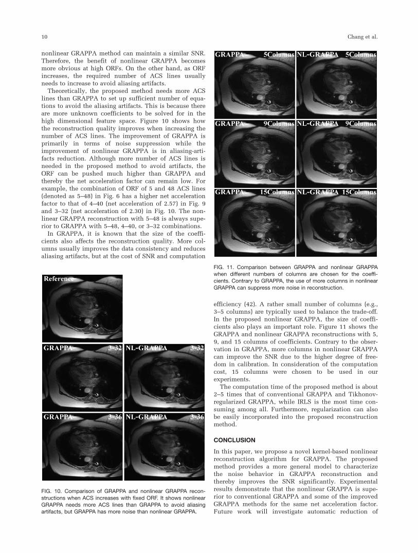
efficiency (42). A rather small number of columns (e.g.,3–5 columns) are typically used to balance the trade-off.In the proposed nonlinear GRAPPA, the size of coeffi-cients also plays an important role. Figure 11 shows theGRAPPA and nonlinear GRAPPA reconstructions with 5,9, and 15 columns of coefficients. Contrary to the obser-vation in GRAPPA, more columns in nonlinear GRAPPAcan improve the SNR due to the higher degree of free-dom in calibration. In consideration of the computationcost, 15 columns were chosen to be used in ourexperiments.

The computation time of the proposed method is about2–5 times that of conventional GRAPPA and Tikhonov-regularized GRAPPA, while IRLS is the most time con-suming among all. Furthermore, regularization can alsobe easily incorporated into the proposed reconstructionmethod.

CONCLUSION

In this paper, we propose a novel kernel-based nonlinearreconstruction algorithm for GRAPPA. The proposedmethod provides a more general model to characterizethe noise behavior in GRAPPA reconstruction andthereby improves the SNR significantly. Experimentalresults demonstrate that the nonlinear GRAPPA is supe-rior to conventional GRAPPA and some of the improvedGRAPPA methods for the same net acceleration factor.Future work will investigate automatic reduction of

FIG. 10. Comparison of GRAPPA and nonlinear GRAPPA recon-structions when ACS increases with fixed ORF. It shows nonlinear

GRAPPA needs more ACS lines than GRAPPA to avoid aliasingartifacts, but GRAPPA has more noise than nonlinear GRAPPA.

FIG. 11. Comparison between GRAPPA and nonlinear GRAPPAwhen different numbers of columns are chosen for the coeffi-cients. Contrary to GRAPPA, the use of more columns in nonlinear

GRAPPA can suppress more noise in reconstruction.

10 Chang et al.

feature space using the methods in Refs. (43–45) toreduce the required number of ACS lines and improvethe computational efficiency. We anticipate that the pro-posed nonlinear approach can bring further benefits tocurrent applications of conventional GRAPPA.

ACKNOWLEDGMENTS

This work was supported in part by the National ScienceFoundation CBET-0731226, CBET-0846514, and a grantfrom the Lynde and Harry Bradley Foundation. Theauthors would like to thank Dr. Edward DiBella for pro-viding the cardiac dataset.

REFERENCES

1. Griswold MA, Jakob PM, Heidemann RM, Mathias Nittka, Jellus V,

Wang J, Kiefer B, Haase A. Generalized autocalibrating partially par-

allel acquisitions (GRAPPA). Magn Reson Med 2002;47:1202–1210.

2. Sodickson DK, Manning WJ. Simultaneous acquisition of spatial har-

monics (SMASH): fast imaging with radiofrequency coil arrays.

Magn Reson Med 1997;38:591–603.

3. Jakob PM, Griswold MA, Edelman RR, Sodickson DK. AutoSMASH: a

self-calibrating technique for SMASH imaging. MAGMA 1998;7:42–54.

4. Pruessmann KP, Weiger M, Scheidegger MB, Boesiger P. SENSE: sen-

sitivity encoding for fast MRI. Magn Reson Med 1999;42:952–962.

5. Griswold MA, Jakob PM, Nittka M, Goldfarb JW, Haase A. Partially

parallel imaging with localized sensitivities (PILS). Magn Reson Med

2000;44:602–609.

6. Kyriakos WE, Panych LP, Kacher DF, Westin CF, Bao SM, Mulkern

RV, Jolesz FA. Sensitivity profiles from an array of coils for encoding

and reconstruction in parallel (SPACE RIP). Magn Reson Med 2000;

44:301–308.

7. Heidemann RM, Griswold MA, Haase A, Jakob PM. VD-AutoSMASH

imaging. Magn Reson Med 2001;45:1066–1074.

8. Yeh EN, McKenzie CA, Ohliger MA, Sodickson DK. Parallel mag-

netic resonance imaging with adaptive radius in k-space (PARS):

constrained image reconstruction using k-space locality in radiofre-

quency coil encoded data. Magn Reson Med 2005;53:1383–1392.

9. Ying L, Sheng J. Joint image reconstruction and sensitivity estimation

in SENSE (JSENSE). Magn Reson Med 2007;57:1196–1202.

10. Park J, Zhang Q, Jellus V, Simonetti O, Li D. Artifact and noise sup-

pression in GRAPPA imaging using improved k-space coil calibration

and variable density sampling. Magn Reson Med 2005;53:186–193.

11. Wang Z, Wang J, Detre JA. Improved data reconstruction method for

GRAPPA. Magn Reson Med 2005;54:738–742.

12. Qu P, Wang C, Shen GX. Discrepancy-based adaptive regularization

for GRAPPA reconstruction. J Magn Reson Imaging 2006;24:248–255.

13. Lin F-H, Prior-Regularized GRAPPA Reconstruction. Proceedings of

the 14th Annual Meeting of ISMRM, Seattle, 2006. p. 3656.

14. Huo D, Wilson D.L. Robust GRAPPA reconstruction and its evalua-

tion with the perceptual difference model. J Magn Reson Imaging

2008;27:1412–1420.

15. Huang F, Li Y, Vijayakumar S, Hertel S, Duensing GR. High-pass

GRAPPA: a image support reduction technique for improved par-

tially parallel imaging. Magn Reson Med 2008;59:642–649.

16. Nana R, Zhao T, Heberlein K, LaConte SM, Hu X. Cross-validation-

based kernel support selection for improved GRAPPA reconstruction.

Magn Reson Med 2008;59:819–825.

17. Nana R and Hu X. Data consistency criterion for selecting parameters

for k-space-based reconstruction in parallel imaging. Magn Reson

Imaging 2010;28, 119–128.

18. Zhao T, Hu X. Iterative GRAPPA (iGRAPPA) for improved parallel

imaging reconstruction. Magn Reson Med 2008;59:903–907.

19. Griswold MA, Blaimer M, Breuer F, Heidemann RM, Mueller M,

Jakob PM. Parallel magnetic resonance imaging using the GRAPPA

operator formalism. Magn Reson Med 2005;54:1553–1556.

20. Bydder M, Jung Y. A nonlinear regularization strategy for GRAPPA

calibration. Magn Reson Imaging 2009;27:137–141.

21. Blaimer M, Gutberlet M, Kellman P, Breuer FA, Kostler H, Griswold

MA. Virtual coil concept for improved parallel MRI employing con-

jugate symmetric signals. Magn Reson Med 2009;61:93–102.

22. Honal M, Bauer S, Ludwig U, Leupold J. Increasing efficiency of par-

allel imaging for 2D multislice acquisitions. Magn Reson Med 2009;

61:1459–1470.

23. Chen Z, Zhang J, Yang R, Kellman P, Johnston LA, Egan GF. IIR

GRAPPA for parallel MR image reconstruction. Magn Reson Med

2010;63:502–509.

24. Wang H, Liang D, King KF, Nagarsekar G, Chang Y, Ying L. Crossed-

Sampled GRAPPA for parallel MRI. Proceedings of the IEEE Engi-

neering in Medicine and Biology Conference, Buenos Aires, Argen-

tina; 2010. p. 3325–3328.

25. Ying L, Abdelsalam E. Parallel MRI Reconstruction: A Filter-Bank

Approach. Proceedings of the IEEE Engineering in Medicine and

Biology Conference, Shanghai, China; 2005. p. 1374–1377.

26. Sharif B, Bresler Y. Distortion-Optimal Self-Calibrating Parallel MRI

by Blind Interpolation in Subsampled Filter Banks. Proceedings of

the IEEE International Symposium on Biomedical Imaging, Chicago,

USA, 2011.

27. Huang F, Duensing GR. A Theoretical Analysis of Errors in GRAPPA.

Proceedings of the 14th Annual Meeting of ISMRM, Seattle; 2006. p.

2468.

28. Carreira-Perpinan MA. Continuous latent variable models for dimen-

sionality reduction and sequential data reconstruction. PhD thesis,

University of Sheffield, UK, 2001.

29. Watkins D. Fundamentals of matrix computations, 2nd ed. New

York, USA: Wiley-Interscience; 2002.

30. Golub G. Some modified matrix eigenvalue problems. SIAM Rev

1973;15:318–344.

31. Golub G, Loan CV. An analysis of the total least squares problem.

SIAM J Numer Anal 1980;17:883–893.

32. Aja-Fernandez S, Tristan-Vega A, Hoge WS, Statistical noise analysis

in GRAPPA using a parameterized noncentral Chi approximation

model. Magn Reson Med 2011;65:1195–1206

33. Tomaso P, Steve S. The mathematics of learning: dealing with data.

Notice Am Math Soc 2003;50:537–544.

34. Liu W, Pokharel PP, Principe JC. The kernel least-mean-square algo-

rithm. IEEE Trans Signal Process 2008;56:543–554.

35. Camps-Valls G, Rojo-Alvarez JL, Martinez-Ramon M. Kernel methods

in bioengineering, signal and image processing. Idea Group Publish-

ing, London, 2007.

36. Schlkopf B, Smola AJ. Learning with kernels: support vector machi-

nesregularizationoptimization and beyond (adaptive computation

and machine learning). The MIT Press: Boston; 2001.

37. Frieb T, Harrison R. A Kernel-Based Adaline. Proceedings of the 7th

European Symposium on Artificial Neural Networks, Bruges, Bel-

gium; 1999. p. 245–250.

38. Kim K, Franz MO, Scholkopf B. Iterative kernel principal component

analysis for image modeling. IEEE Trans Pattern Anal Machine Intell

2005;27:1351–1366.

39. Chang YW, Hsieh CJ, Chang KW, Ringgaard M, Lin CJ. Training and

testing low-degree polynomial data mappings via linear SVM. J

Machine Learn Res 2010;11:1471–1490.

40. Zhang T. Learning bounds for kernel regression using effective data

dimensionality. Neural Comput 2005;17:2077–2098.

41. Robson PM, Grant AK, Madhuranthakam AJ, Lattanzi R, Sodickson

DK, McKenzie CA. Comprehensive quantification of signal-to-noise

ratio and g-factor for image-based and k-space-based parallel imaging

reconstructions. Magn Reson Med 2008;60:895–907.

42. Bauer S, Markl M, Honal M, Jung BA. The effect of reconstruction

and acquisition parameters for GRAPPA-based parallel imaging on

the image quality. Magn Reson Med 2011; March, Early View

Online.

43. Doneva M, Bornert P. Automatic coil selection for channel reduction

in SENSE-based parallel imaging. MAGMA 2008;21(3):187–196.

44. Huang F, Vijayakumar S, Li Y, Hertel S, Duensing GR. A software

channel compression technique for faster reconstruction with many

channels. Magn Reson Imaging 2008;26:133–141.

45. Feng S, Zhu Y, Ji J. Efficient large-array k-domain parallel MRI using

channel-by-channel array reduction. Magn Reson Imaging 2011;29:

209–215.

Nonlinear GRAPPA 11