Nonlinear geometric analysis on Finsler manifolds

Shin-ichi Ohta∗

Abstract

This is a survey article on recent progress of comparison geometry and geomet-ric analysis on Finsler manifolds of weighted Ricci curvature bounded below. Ourpurpose is two-fold: Give a concise and geometric review on the birth of weightedRicci curvature and its applications; Explain recent results from a nonlinear ana-logue of the Γ-calculus based on the Bochner inequality. In the latter we discusssome gradient estimates, functional inequalities, and isoperimetric inequalities.

Contents

1 Introduction 2

2 Comparison geometry of Finsler manifolds 42.1 Finsler structures . . . . . . . . . . . . . . . . . . . . . . . . . . . . . . . . 42.2 Asymmetric distance and geodesics . . . . . . . . . . . . . . . . . . . . . . 62.3 Covariant derivative . . . . . . . . . . . . . . . . . . . . . . . . . . . . . . 82.4 Curvatures . . . . . . . . . . . . . . . . . . . . . . . . . . . . . . . . . . . . 92.5 Weighted Ricci curvature . . . . . . . . . . . . . . . . . . . . . . . . . . . . 10

3 Nonlinear Laplacian and heat semigroup 133.1 Gradient vectors, Hessian and Laplacian . . . . . . . . . . . . . . . . . . . 133.2 Bochner–Weitzenbock formula . . . . . . . . . . . . . . . . . . . . . . . . . 153.3 Heat equation . . . . . . . . . . . . . . . . . . . . . . . . . . . . . . . . . . 16

4 Linearized heat semigroups and gradient estimates 174.1 Linearized heat semigroups and their adjoints . . . . . . . . . . . . . . . . 184.2 Gradient estimates . . . . . . . . . . . . . . . . . . . . . . . . . . . . . . . 194.3 Characterizations of lower Ricci curvature bounds . . . . . . . . . . . . . . 21

5 Functional inequalities 215.1 Poincare–Lichnerowicz inequality . . . . . . . . . . . . . . . . . . . . . . . 225.2 Logarithmic Sobolev inequality . . . . . . . . . . . . . . . . . . . . . . . . 235.3 Sobolev inequalities . . . . . . . . . . . . . . . . . . . . . . . . . . . . . . . 25

∗Department of Mathematics, Kyoto University, Kyoto, 606-8502, Japan (sohta@math.kyoto-u.ac.jp), Current address: Department of Mathematics, Osaka University, Osaka, 560-0043, Japan(s.ohta@math.sci.osaka-u.ac.jp); Supported in part by JSPS Grant-in-Aid for Scientific Research (KAK-ENHI) 15K04844.

1

6 Gaussian isoperimetric inequality 286.1 Background for Levy–Gromov isoperimetic inequality . . . . . . . . . . . . 296.2 Isoperimetric inequality . . . . . . . . . . . . . . . . . . . . . . . . . . . . . 30

1 Introduction

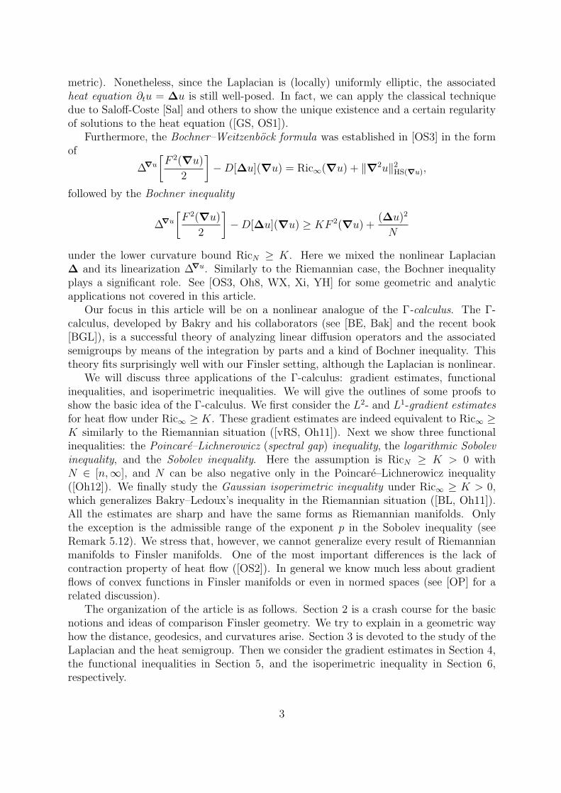
The aim of this article is to review the recent developments of comparison geometryand geometric analysis on Finsler manifolds of weighted Ricci curvature bounded below.The weighted Ricci curvature was introduced by the author in [Oh3]. Since then it hashelped us to understand the similarities and differences between Riemannian and Finslermanifolds more deeply. One of the main challenges, compared with the Riemannian case,is in the nonlinearity of the Laplacian and the associated heat equation. How to deal withsuch a nonlinear evolution equation would be of interest also in the analytic viewpoint.

A Finsler manifold will be a pair of a manifoldM and a nonnegative function F on thetangent bundle TM such that F |TxM gives a Minkowski norm for each x ∈M . We remarkthat F (−v) = F (v) is allowed, which is called the non-reversibility and is a special featureof Finsler manifolds. One can define the distance and geodesics in natural geometric ways,whereas the non-reversibility of F leads to the asymmetry of the distance, namely d(y, x)does not necessarily coincide with d(x, y). Analyzing the behavior of geodesics, we canfurther introduce Jacobi fields and the curvature tensor. Thus we arrive at the naturalnotions of the flag curvature (a generalization of the Riemannian sectional curvature) andthe Ricci curvature. Some results in comparison Riemannian geometry concerning thedistance are then generalized to the Finsler context (for example, the Cartan–Hadamardtheorem and the Bonnet–Myers theorem).

Now, to proceed further in this direction, what is ameasure controlled by the Ricci cur-vature? At this point we have another difficulty; There are several choices for a ‘canonical’measure (such as the Busemann–Hausdorff measure and the Holmes–Thompson measure),all of them go down to the volume measure on a Riemannian manifold. Our strategy ini-tiated in [Oh3] is that, instead of choosing some constructive measure, we begin withan arbitrary (smooth, positive) measure m on M and modify the Ricci curvature ac-cording to the choice of m. The modification is done in the same manner as weightedRiemannian manifolds. We call this modified Ricci curvature the weighted Ricci cur-vature RicN (also called the Bakry–Emery–Ricci curvature), where N is a parametersometimes called the effective dimension. By means of RicN , one can generalize many re-sults including the Bishop–Gromov volume comparison to this Finsler context and, mostnotably, the curvature-dimension condition CD(K,N) in the sense of Lott–Sturm–Villani([St1, St2, LV]) is equivalent to the lower curvarture bound RicN ≥ K ([Oh3]). Thisdeep equivalence relation ensures the naturalness and importance of the weighted Riccicurvature.

The Ricci curvature plays the prominent role in geometric analysis. The Laplacian ∆acting on functions is naturally defined as the divergence (in terms of m) of the gradientvector field (in terms of F ). This is also called the Witten Laplacian or the weightedLaplacian. Since taking the gradient vector (more precisely, the Legendre transform) isa nonlinear operation, our Laplacian is nonlinear (unless F comes from a Riemannian

2

metric). Nonetheless, since the Laplacian is (locally) uniformly elliptic, the associatedheat equation ∂tu = ∆u is still well-posed. In fact, we can apply the classical techniquedue to Saloff-Coste [Sal] and others to show the unique existence and a certain regularityof solutions to the heat equation ([GS, OS1]).

Furthermore, the Bochner–Weitzenbock formula was established in [OS3] in the formof

∆∇u

[F 2(∇u)

2

]−D[∆u](∇u) = Ric∞(∇u) + ∥∇2u∥2HS(∇u),

followed by the Bochner inequality

∆∇u

[F 2(∇u)

2

]−D[∆u](∇u) ≥ KF 2(∇u) +

(∆u)2

N

under the lower curvature bound RicN ≥ K. Here we mixed the nonlinear Laplacian∆ and its linearization ∆∇u. Similarly to the Riemannian case, the Bochner inequalityplays a significant role. See [OS3, Oh8, WX, Xi, YH] for some geometric and analyticapplications not covered in this article.

Our focus in this article will be on a nonlinear analogue of the Γ-calculus. The Γ-calculus, developed by Bakry and his collaborators (see [BE, Bak] and the recent book[BGL]), is a successful theory of analyzing linear diffusion operators and the associatedsemigroups by means of the integration by parts and a kind of Bochner inequality. Thistheory fits surprisingly well with our Finsler setting, although the Laplacian is nonlinear.

We will discuss three applications of the Γ-calculus: gradient estimates, functionalinequalities, and isoperimetric inequalities. We will give the outlines of some proofs toshow the basic idea of the Γ-calculus. We first consider the L2- and L1-gradient estimatesfor heat flow under Ric∞ ≥ K. These gradient estimates are indeed equivalent to Ric∞ ≥K similarly to the Riemannian situation ([vRS, Oh11]). Next we show three functionalinequalities: the Poincare–Lichnerowicz (spectral gap) inequality, the logarithmic Sobolevinequality, and the Sobolev inequality. Here the assumption is RicN ≥ K > 0 withN ∈ [n,∞], and N can be also negative only in the Poincare–Lichnerowicz inequality([Oh12]). We finally study the Gaussian isoperimetric inequality under Ric∞ ≥ K > 0,which generalizes Bakry–Ledoux’s inequality in the Riemannian situation ([BL, Oh11]).All the estimates are sharp and have the same forms as Riemannian manifolds. Onlythe exception is the admissible range of the exponent p in the Sobolev inequality (seeRemark 5.12). We stress that, however, we cannot generalize every result of Riemannianmanifolds to Finsler manifolds. One of the most important differences is the lack ofcontraction property of heat flow ([OS2]). In general we know much less about gradientflows of convex functions in Finsler manifolds or even in normed spaces (see [OP] for arelated discussion).

The organization of the article is as follows. Section 2 is a crash course for the basicnotions and ideas of comparison Finsler geometry. We try to explain in a geometric wayhow the distance, geodesics, and curvatures arise. Section 3 is devoted to the study of theLaplacian and the heat semigroup. Then we consider the gradient estimates in Section 4,the functional inequalities in Section 5, and the isoperimetric inequality in Section 6,respectively.

3

Acknowledgements. I thank Professor Sorin Sabau for encouraging me to write a surveyon this subject. I am also grateful to an anonymous referee for valuable comments.

2 Comparison geometry of Finsler manifolds

This section is devoted to a concise review on comparison geometry of Finsler manifolds.The main object will be a Finsler manifold equipped with a measure whose weighted Riccicurvature is bounded from below. We refer to [BCS, Sh2, SS] for the fundamentals ofFinsler geometry as well as related comparison geometric studies.

Throughout the article, unless otherwise indicated, letM be a connected C∞-manifoldwithout boundary of dimension n ≥ 2. We will also fix an arbitrary positive C∞-measurem on M from Subsection 2.5.

2.1 Finsler structures

Given local coordinates (xi)ni=1 on an open set U ⊂ M , we will always use the fiber-wiselinear coordinates (xi, vj)ni,j=1 of TU such that

v =n∑

j=1

vj∂

∂xj

∣∣∣x∈ TxM, x ∈ U.

Definition 2.1 (Finsler structures) We say that a nonnegative function F : TM −→[0,∞) is a C∞-Finsler structure of M if the following three conditions hold:

(1) (Regularity) F is C∞ on TM \ 0, where 0 stands for the zero section;

(2) (Positive 1-homogeneity) It holds F (cv) = cF (v) for all v ∈ TM and c ≥ 0;

(3) (Strong convexity) The n× n matrix

(gij(v)

)ni,j=1

:=

(1

2

∂2(F 2)

∂vi∂vj(v)

)n

i,j=1

(2.1)

is positive-definite for all v ∈ TM \ 0.

We call such a pair (M,F ) a C∞-Finsler manifold.

Notice that the positive-definiteness is independent of the choice of local coordinates.One can similarly define Cl-Finsler manifolds, though we consider only C∞-Finsler mani-folds in this article. Some more remarks on Definition 2.1 are ready.

Remark 2.2 (a) The homogeneity (2) is imposed only in the positive direction, that is,for nonnegative c. This leads to the asymmetry of the associated distance function (seethe next subsection). If F (−v) = F (v) holds for all v ∈ TM , then we say that F isreversible or absolutely homogeneous.

(b) The strong convexity (3) means that the unit sphere UxM := TxM ∩ F−1(1)(called the indicatrix ) is positively curved, and it implies the strict convexity: F (v+w) ≤

4

F (v)+F (w) for all v, w ∈ TxM and equality holds only when v = aw or w = av for somea ≥ 0.

(c) Although we will discuss only under Definition 2.1, the C∞-regularity (1) and thestrong convexity (3) can be weakened in various ways occasionally (see [OS1] for instance).

Let us continue the study of the strong convexity in the remainder of this subsection.Given each v ∈ TxM \ 0, the positive-definite matrix (gij(v))

ni,j=1 in (2.1) induces the

Riemannian structure gv of TxM as

gv

( n∑i=1

ai∂

∂xi

∣∣∣x,

n∑j=1

bj∂

∂xj

∣∣∣x

):=

n∑i,j=1

gij(v)aibj. (2.2)

Notice that this definition is coordinate-free, and we have gv(v, v) = F 2(v). One canregard gv as the best Riemannian approximation of F |TxM in the direction v. In fact,the unit sphere of F |TxM (which is positively curved due to Remark 2.2(b)) is tangent tothat of gv at v/F (v) up to the second order. The metric gv plays quite important roles incomparison Finsler geometry.

In the coordinates (xi, αj)ni,j=1 of T ∗U given by α =

∑nj=1 αjdx

j, we will also consider

g∗ij(α) :=1

2

∂2[(F ∗)2]

∂αi∂αj

(α), i, j = 1, 2, . . . , n,

for α ∈ T ∗U \ 0. Here F ∗ : T ∗M −→ [0,∞) is the dual Minkowski norm to F , namely

F ∗(α) := supv∈TxM,F (v)≤1

α(v) = supv∈TxM,F (v)=1

α(v)

for α ∈ T ∗xM . It is clear by definition that α(v) ≤ F ∗(α)F (v), and hence

α(v) ≥ −F ∗(α)F (−v), α(v) ≥ −F ∗(−α)F (v).

We remark and stress that, however, α(v) ≥ −F ∗(α)F (v) does not hold in general due tothe non-reversibility of F .

The strong convexity is related to the following quantities, these are fundamental inthe geometry of Banach spaces (see [BCL, Oh2]). For x ∈ M , we define the (2-)uniformsmoothness constant at x by

SF (x) := supv,w∈TxM\0

gv(w,w)

F 2(w)= sup

α,β∈T ∗xM\0

F ∗(β)2

g∗α(β, β).

Since gv(w,w) ≤ SF (x)F2(w) and gv is the Hessian of F 2/2 at v, the constant SF (x)

measures the concavity of F 2 in TxM . We also set SF := supx∈M SF (x). Notice thatSF ∈ [1,∞] and SF = 1 holds if and only if F comes from a Riemannian metric (see[Oh2]). We similarly define the (2-)uniform convexity constants as

CF (x) := supv,w∈TxM\0

F 2(w)

gv(w,w)= sup

α,β∈T ∗xM\0

g∗α(β, β)

F ∗(β)2, CF := sup

x∈MCF (x).

5

Again, CF ∈ [1,∞] in general and CF = 1 holds if and only if (M,F ) is Riemannian.It is readily seen that the constants SF and CF control the reversibility constant,

defined by

ΛF := supv∈TM\0

F (v)

F (−v)∈ [1,∞],

as follows (see [Oh11, Lemma 2.4] for instance).

Lemma 2.3 We haveΛF ≤ min{

√SF ,

√CF}.

For later convenience, we introduce the following notations.

Definition 2.4 (Reverse Finsler structures) We define the reverse Finsler structure←−F of F by

←−F (v) := F (−v). We will put an arrow ← on those quantities associated with

←−F .

For example,←−d(x, y) = d(y, x) (see §2.2),

←−Ric(v) = Ric(−v) (§2.4),

←−RicN(v) =

RicN(−v) (§2.5),←−∇u = −∇(−u) and

←−∆u = −∆(−u) (§3.1).

2.2 Asymmetric distance and geodesics

For x, y ∈M , we define the (asymmetric) distance from x to y by

d(x, y) := infη

∫ 1

0

F(η(t)

)dt,

where the infimum is taken over all piecewise C1-curves η : [0, 1] −→M such that η(0) = xand η(1) = y. Note that the asymmetry d(y, x) = d(x, y) can occur since F is onlypositively homogeneous (so d is not properly a distance function in the usual sense). Wealso remark that the squared distance function d2(x, ·) is only C1 at x in general, and thatd2(x, ·) is C2 at x for all x ∈ M if and only if F comes from a Riemannian metric (see[Sh1, Proposition 2.2]). This is a reason why we have the less regularity for heat flow (seeTheorem 3.7 below).

In the manner of metric geometry, we say that a C∞-curve η : I −→ M from aninterval I ⊂ R is geodesic if it is locally minimizing and has a constant speed with respectto d. Precisely, there is C ≥ 0 and, for any t ∈ I, we find ε > 0 such that

d(η(s), η(s′)

)= C(s′ − s)

for all s, s′ ∈ I ∩ [t− ε, t+ ε] with s ≤ s′ (then F (η) ≡ C as a matter of course).One can write down the geodesic equation as the Euler–Lagrange equation for the ac-

tion induced from F 2. In such calculations, the following basic theorem plays fundamentalroles (see [BCS, Theorem 1.2.1]).

6

Theorem 2.5 (Euler’s homogeneous function theorem) Consider a differentiablefunction H : Rn \ {0} −→ R satisfying H(cv) = crH(v) for some r ∈ R and all c > 0 andv ∈ Rn \ {0} (that is, H is positively r-homogeneous). Then we have

n∑i=1

∂H

∂vi(v)vi = rH(v)

for all v ∈ Rn \ {0}.

Observe that gij defined in (2.1) is positively 0-homogeneous on each TxM , and hence

n∑i=1

Aijk(v)vi =

n∑j=1

Aijk(v)vj =

n∑k=1

Aijk(v)vk = 0 (2.3)

for all v ∈ TM \ 0 and i, j, k = 1, 2, . . . , n, where

Aijk(v) :=F (v)

2

∂gij∂vk

(v), v ∈ TM \ 0,

is the Cartan tensor which measures the variation of gv in the vertical directions. TheCartan tensor vanishes everywhere on TM \ 0 if and only if F comes from a Riemannianmetric. In this sense, the Cartan tensor is a genuinely non-Riemannian quantity.

With the help of (2.3), we arrive at the following geodesic equation by the usualcalculation similar to the Riemannian case:

ηi(t) +n∑

j,k=1

γijk(η(t)

)ηj(t)ηk(t) = 0 (2.4)

for all i, where

γijk(v) :=1

2

n∑l=1

gil(v)

{∂glk∂xj

(v) +∂gjl∂xk

(v)− ∂gjk∂xl

(v)

}, v ∈ TM \ 0, (2.5)

is called the formal Christoffel symbol. We denoted by (gij(v)) the inverse matrix of(gij(v)). Notice that γijk has the same form as the Riemannian Christoffel symbol, whileit is a (0-homogeneous) function on TM \ 0 and cannot be reduced to a function on M .

By the general ODE theory, every initial vector v ∈ TM admits a unique geodesicη : (−ε, ε) −→ M with η(0) = v for some ε > 0. Given v ∈ TxM , if there is a geodesicη : [0, 1] −→ M with η(0) = v, then we define the exponential map by expx(v) := η(1).We say that (M,F ) is forward complete if the exponential map is defined on whole TM .In other words, every geodesic η : [0, 1] −→ M is extended infinitely in the forwarddirection to the geodesic η : [0,∞) −→ M . If every geodesic η : [0, 1] −→ M is extended

in the backward direction to the geodesic η : (−∞, 1] −→ M (in other words, if (M,←−F )

is forward complete), then we say that (M,F ) is backward complete. The backwardcompleteness is not necessarily equivalent to the forward completeness (in the noncompactcase). If (M,F ) is forward or backward complete, then the Hopf–Rinow theorem ensuresthat any pair of points is connected by a minimal geodesic (see [BCS, Theorem 6.6.1]).

7

2.3 Covariant derivative

We saw in (2.4) and (2.5) that the Finsler geodesic equation has a similar form to theRiemannian one. This is, however, a special feature of the geodesic equation and we needto take care of some non-Riemannian quantities in the more general covariant derivative.A fine property of the geodesic equation could be understood from Theorem 2.5. In orderto apply Theorem 2.5 to some quantity at v ∈ TM \0, we need a contraction with respectto v. In the geodesic equation (2.4) we have the contractions twice thanks to ηj(t) andηk(t), this procedure kills all the error (non-Riemannian) terms.

Notice that the geodesic equation for the Riemannian structure gη (defined only alongη) coincides with the geodesic equation (2.4) with respect to F . This kind of property isextremely useful when we try to apply the techniques in Riemannian geometry to Finslergeometry. This viewpoint leads us to modify the formal Christoffel symbol (2.5) into

Γijk(v) := γijk(v)−

n∑l,m=1

gil

F(AlkmN

mj + AjlmN

mk − AjkmN

ml )(v), v ∈ TM \ 0, (2.6)

where

N ij(v) :=

1

2

∂Gi

∂vj(v), Gi(v) :=

n∑j,k=1

γijk(v)vjvk

(the validity of the definition (2.6) can be seen in Proposition 2.6 below). We call Gi

and N ij the geodesic spray coefficients and the nonlinear connection, respectively, and set

Gi(0) = N ij(0) := 0 by convention. Notice that (2.3) yields

n∑j,k=1

Γijk(v)v

jvk =n∑

j,k=1

γijk(v)vjvk.

However, when we contract in v only once,n∑

j=1

{Γijk(v)− γijk(v)}vj = −

n∑l,m=1

gil(v)

F (v)Alkm(v)G

m(v)

does not necessarily vanish.Define the covariant derivative of a vector field X by v ∈ TxM with the reference

vector w ∈ TxM \ 0 as

Dwv X(x) :=

n∑i,j=1

{vj∂X i

∂xj(x) +

n∑k=1

Γijk(w)v

jXk(x)

}∂

∂xi

∣∣∣x∈ TxM. (2.7)

With this definition, we can show the following important property (see [Sh2, §6.2] or[Oh8, Lemma 2.3]).

Proposition 2.6 Let V be a non-vanishing C∞-vector field on an open set U such thatall integral curves are geodesic. Then we have, for any C1-vector field W on U ,

DVVW = DgV

V W, DVWV = DgV

W V.

Here gV is the Riemannian structure of U induced from V as (2.2) and DgV denotes itscorresponding covariant derivative.

8

In particular, integral curves of V are geodesic also with respect to gV . Note thatwe have only one contraction (with respect to V ) in DV

VW and DVWV . The geodesic

equation Dηη η ≡ 0 is concerned with the special case of W = V , where we have one more

contraction.

2.4 Curvatures

In order to define the curvature, we again look at the behavior of geodesics. It can beshown that the variational vector field J of a geodesic variation σ : [0, 1]× (−ε, ε) −→M(i.e., σ(·, s) is geodesic for all s and J(t) := ∂σ/∂s(t, 0)) satisfies the Jacobi equation

DηηD

ηηJ +Rη(J) = 0 (2.8)

and vice versa, where η(t) := σ(t, 0) and

Rv(w) :=n∑

i,j=1

Rij(v)w

j ∂

∂xi

∣∣∣x,

Rij(v) :=

∂Gi

∂xj(v)−

n∑k=1

{∂N i

j

∂xk(v)vk −

∂N ij

∂vk(v)Gk(v)

}−

n∑k=1

N ik(v)N

kj (v).

We refer to [Sh2, §6.1] for details (where Gi is one-half of ours, while N ij is the same). It

is unnecessary to worry about the complicated formula of Rij(v), what we essentially need

will be only the Jacobi equation (2.8) and the characterization in Theorem 2.10 below.

Definition 2.7 (Flag curvature) For linearly independent vectors v, w ∈ TxM , we de-fine the flag curvature by

K(v, w) :=gv(Rv(w), w)

F 2(v)gv(w,w)− gv(v, w)2.

On Riemannian manifolds, the flag curvature K(v, w) coincides with the sectionalcurvature of the 2-plane v ∧ w spanned by v and w. We remark that K(v, w) dependsnot only on the flag v ∧ w, but also on the choice of the pole v in it. Thus, for example,K(w, v) may be different from K(v, w). We further define the Ricci curvature as follows.

Definition 2.8 (Ricci curvature) For a unit vector v ∈ UxM , we define the Riccicurvature as the trace of the flag curvature with respect to gv, namely

Ric(v) :=n−1∑i=1

K(v, ei),

where {ei}n−1i=1 ∪{v} is orthonormal with respect to gv. We also define Ric(cv) := c2Ric(v)

for c ≥ 0.

As usual, given K ∈ R, the bound Ric ≥ K will mean that Ric(v) ≥ KF 2(v) holds

for all v ∈ TM . We remark that this curvature bound is common to F and←−F since one

can see←−Ric(v) = Ric(−v) from Theorem 2.10 (recall Definition 2.4 for the definitions of

←−F and

←−Ric).

9

Remark 2.9 The appropriate notion of scalar curvature is still missing in the Finslersetting. This is one of the main obstructions to develop the theory of Finsler–Ricci flow.

Comparing Proposition 2.6 and (2.8), one finds the following quite important anduseful property.

Theorem 2.10 (A Riemannian characterization of Finsler curvatures) Given aunit vector v ∈ UxM , take a C∞-vector field V on a neighborhood U of x such thatV (x) = x and all integral curves of V are geodesic. Then, for any w ∈ TxM linearly in-dependent from v, the flag curvature K(v, w) coincides with the sectional curvature of the2-plane v∧w with respect to the Riemannian metric gV on U . Similarly, Ric(v) coincideswith the Ricci curvature of v with respect to gV .

We in particular find that the sectional curvature of v∧w with respect to gV does notdepend on the choice of V , where the assumption on V (all integral curves are geodesic)is playing the essential role. The proof of Theorem 2.10 can be found in [Sh2, §6], whichinspired the structure of this section. The characterization in the manner of Theorem 2.10goes back to at least [Au].

Via Theorem 2.10, one can reduce some results on Finsler manifolds to the Riemanniancase. The most fundamental ones are the following (obtained in [Au]), we will see somemore (concerning the weighted Ricci curvature) in the next subsection.

Theorem 2.11 (Cartan–Hadamard theorem) Let (M,F ) be a simply-connected andforward complete Finsler manifold with nonpositive flag curvature K ≤ 0. Then theexponential map expx : TxM −→M is a C1-diffeomorphism for every x ∈M .

Theorem 2.12 (Bonnet–Myers theorem) If (M,F ) is forward complete and satisfiesRic ≥ K for some K > 0, then we have

diam(M) := supx,y∈M

d(x, y) ≤ π

√n− 1

K.

In particular, M is compact.

Outline of proof. Let us outline the proof of Theorem 2.12 (Theorem 2.11 is shown in asimilar manner). Fix a point x ∈ M and consider unit speed geodesics η : [0, lη) −→ Memanating from x. Here lη ∈ (0,∞) is taken as the supremum of t > 0 such thatd(x, η(t)) = t. Define the vector field V by V (η(t)) := η(t) for each η and t ∈ (0, lη).Then V is a C∞-vector field on an open set U ⊂M\{x} and all integral curves are geodesic.Thanks to Theorem 2.10, the Riemannian metric gV has the Ricci curvature ≥ K. There-fore the Riemannian Bonnet–Myers theorem applies and we have lη ≤ π

√(n− 1)/K.

This shows the claim. 2

2.5 Weighted Ricci curvature

In order to discuss further applications of the Ricci curvature, it is natural to employ asuitable measure on M . At this point, our Finsler setting has another difficulty that the

10

choice of a canonical measure is not unique. There are several known ways to generalizethe Riemannian volume measure, canonical in their own rights, leading to the differentmeasures. Among others the most fundamental examples of constructive measures arethe Busemann–Hausdorff measure and the Holmes–Thompson measure (see [AT]).

Our standpoint is that, instead of starting from a constructive measure, we consideran arbitrary measure (this turns out natural, see Remark 2.15). Then, inspired by Theo-rem 2.10 as well as the theory of weighted Ricci curvature (also called the Bakry–Emery–Ricci curvature) of Riemannian manifolds, one can define the weighted Ricci curvature asin [Oh3]. From here on, we fix a positive C∞-measure m on M (meaning that it is writtendown as m = Φ dx1 · · · dxn in each local coordinates with some positive C∞-function Φ).

Definition 2.13 (Weighted Ricci curvature) Given a unit vector v ∈ UxM , let Vbe a non-vanishing C∞-vector field on a neighborhood U of x such that V (x) = v andall integral curves of V are geodesic. We decompose m as m = e−Ψ volgV on U , whereΨ ∈ C∞(U) and volgV is the volume measure of gV . Denote by η : (−ε, ε) −→ M thegeodesic such that η(0) = v. Then, for N ∈ (−∞, 0) ∪ (n,∞), define

RicN(v) := Ric(v) + (Ψ ◦ η)′′(0)− (Ψ ◦ η)′(0)2

N − n.

We also define as the limits:

Ric∞(v) := Ric(v) + (Ψ ◦ η)′′(0), Ricn(v) := limN↓n

RicN(v).

Finally, for c ≥ 0, we set RicN(cv) := c2RicN(v).

We will denote by RicN ≥ K, K ∈ R, the condition RicN(v) ≥ KF 2(v) for all v ∈ TM .Some remarks on Definition 2.13 are in order.

Remark 2.14 (a) In local coordinates, volgV along η is written as√det(gij

(η))dx1 · · · dxn.

Hence we find

Ψ(η) = log

(√det(gij(η))

Φ(η)

), where m = Φ dx1 · · · dxn.

This expression does not require the vector field V (though we introduced it for the sakeof lucidity), thereby Ψ ◦ η does not depend on the choice of V .

(b) On a Riemnnian manifold (M, g), the metric gV always coincides with the originalmetric g and hence Ψ is regarded as a function onM such that m = e−Ψ volg. If we choosem = volg, then RicN = Ric regardless of the choice of N .

(c) Multiplying the measure m with a positive constant does not change the weightedRicci curvature. Therefore we can freely normalize m as m(M) = 1 when m(M) <∞.

(d) Notice that RicN is non-decreasing in N in the ranges [n,∞] and (−∞, 0), and wehave

Ricn ≤ RicN ≤ Ric∞ ≤ RicN ′ for N ∈ (n,∞), N ′ < 0.

11

Therefore, RicN ′ ≥ K with N ′ < 0 is a weaker condition than RicN ≥ K for N ∈ (n,∞).In the Riemannian case, the study of Ric∞ goes back to Lichnerowicz [Li], he showed aCheeger–Gromoll type splitting theorem (see [FLZ, WW, Oh8] for some generalizations).The range N ∈ (n,∞) has been well investigated by Bakry [Bak, §6], Qian [Qi] andmany others. The study of the range N ∈ (−∞, 0) is more recent. We refer to [Mi2]for isoperimetric inequalities, [Oh9, Oh10] for the curvature-dimension condition (withN ≤ 0), and [Wy] for splitting theorems (with N ∈ (−∞, 1]). Some historical accountson related works concerning N < 0 in convex geometry and partial differential equationscan be found in [Mi2, Mi3].

Related to (b) above, a reason why we consider it natural to begin with an arbitrarymeasure is explained as follows.

Remark 2.15 (S-curvature) For Finsler manifolds of Berwald type (i.e., Γkij is constant

on each TxM \0), the Busemann–Hausdorff measure satisfies (Ψ◦η)′ ≡ 0 (in other words,the S-curvature vanishes, see [Sh2, §7.3]). In general, however, there may not existany measure whose S-curvature vanishes (see [Oh5] for such an example among Randersspaces). We regard this fact as the non-existence of a canonical measure, thus we beganwith an arbitrary measure.

The weighted version of the Bonnet–Myers theorem (Theorem 2.12) can be shown inthe same manner as the unweighted case.

Theorem 2.16 (Bonnet–Myers theorem) If (M,F,m) is forward complete and sat-isfies RicN ≥ K for some K > 0 and N ∈ [n,∞), then we have

diam(M) ≤ π

√N − 1

K.

In particular, M is compact.

From this estimate N can be regarded as (an upper bound of) the dimension (thoughthis interpretation prevents us from considering N < 0). We can further control thevolume growth for m. For x ∈M and r > 0, we define

B+(x, r) := {y ∈M | d(x, y) < r}.

We also introduce the function sκ defined by

sκ(θ) :=

1√κsin(√κθ) if κ > 0,

θ if κ = 0,1√−κ

sinh(√−κθ) if κ < 0,

where θ ≥ 0 if κ ≤ 0 and θ ∈ [0, π/√κ] if κ > 0.

Theorem 2.17 (Bishop–Gromov volume comparison) Suppose that (M,F,m) isforward complete and satisfies RicN ≥ K for some K ∈ R and N ∈ [n,∞). Thenwe have

m(B+(x,R))

m(B+(x, r))≤

∫ R

0sK/(N−1)(t)

N−1 dt∫ r

0sK/(N−1)(t)N−1 dt

12

for any x ∈M and 0 < r < R, where R ≤ π√

(N − 1)/K if K > 0.

Note that the condition R ≤ π√

(N − 1)/K for K > 0 does not lose any generality be-cause of Theorem 2.16. Similarly to Theorems 2.11, 2.12, 2.16, the proof of Theorem 2.17can be reduced to the (weighted) Riemannian situation by employing the Riemannianmetric induced from the unit speed geodesics emanating from x.

Remark 2.18 (Curvature-dimension condition) The original motivation of intro-ducing RicN in [Oh3] was to study Lott, Sturm and Villani’s curvature-dimension condi-tion CD(K,N) on Finsler manifolds (see also the surveys [Oh4, Oh6]). The celebratedcondition CD(K,N) was introduced as a synthetic geometric notion playing a role ofa lower Ricci curvature bound for metric measure spaces ([St1, St2, LV]). On a com-plete Riemannian manifold with an arbitrary measure (M, g,m), the condition CD(K,N)is indeed equivalent to RicN ≥ K (see [vRS, St1, St2, LV], where N ∈ [n,∞]). In[Oh3] this equivalence was generalized to Finsler manifolds (M,F,m), with applicationsincluding the Bishop–Gromov volume comparison and some functional inequalities (seealso Section 5 for the latter). As we have already mentioned in Remark 2.14(d), thecurvature-dimension condition can be extended to N ∈ (−∞, 0] and is again equivalentto RicN ≥ K ([Oh9, Oh10]).

The theory of metric measure spaces satisfying CD(K,N) is making a deep and breath-taking progress in this decade. We refer to Villani’s book [Vi] as a fundamental refer-ence, and Cavalletti–Mondino’s Levy–Gromov type isoperimetric inequalities ([CM1], seealso Section 6) as one of the most notable achievements after [Vi]. Since the conditionCD(K,N) could not rule out Finsler manifolds, a reinforced version of CD(K,N) coupledwith the linearity of the heat semigroup was introduced and is called the Riemanniancurvature-dimension condition RCD(K,N) ([AGS, EKS]). In this Riemannian frame-work, many finer results such as Gigli’s splitting theorem [Gi1] and second order calculus[Gi2] as well as Mondino–Naber’s rectifiability [MN] are known.

3 Nonlinear Laplacian and heat semigroup

At this section we begin geometric analysis on Finsler manifolds. The main object of thesection is the Bochner–Weitzenbock formula (Theorem 3.3), which is the indispensableingredient of our nonlinear analogue of the Γ-calculus.

3.1 Gradient vectors, Hessian and Laplacian

Let us denote by L∗ : T ∗M −→ TM the Legendre transform associated with F . That isto say, L∗ is sending α ∈ T ∗

xM to the unique element v ∈ TxM such that F (v) = F ∗(α)and α(v) = F ∗(α)2. In coordinates we can write down

L∗(α) =n∑

i,j=1

g∗ij(α)αj∂

∂xi

∣∣∣x=

n∑i=1

1

2

∂[(F ∗)2]

∂αi

(α)∂

∂xi

∣∣∣x

for α ∈ T ∗xM \ 0 (the latter expression makes sense also at 0 as L∗(0) = 0). Note that

g∗ij(α) = gij(L∗(α)

)for α ∈ T ∗

xM \ 0

13

(recall that (gij(v)) denotes the inverse matrix of (gij(v))). The map L∗|T ∗xM is being a

linear operator only when F |TxM comes from an inner product.For a differentiable function u : M −→ R, the gradient vector at x is defined as the

Legendre transform of the derivative of u: ∇u(x) := L∗(Du(x)) ∈ TxM . If Du(x) = 0,then we can write down in coordinates as

∇u(x) =n∑

i,j=1

g∗ij(Du(x)

) ∂u∂xj

(x)∂

∂xi

∣∣∣x.

We need to be careful when Du(x) = 0, because g∗ij(Du(x)) is not defined as well as theLegendre transform L∗ is only continuous at the zero section. Thus we set for later use

Mu := {x ∈M |Du(x) = 0}.

For a twice differentiable function u :M −→ R and x ∈Mu, we define a kind of Hessian∇2u(x) : TxM −→ TxM by using the covariant derivative (2.7) as

∇2u(v) := D∇uv (∇u)(x) ∈ TxM, v ∈ TxM.

The linear operator ∇2u(x) is symmetric in the sense that

g∇u

(∇2u(v), w

)= g∇u

(v,∇2u(w)

)for all v, w ∈ TxM with x ∈Mu (see, for example, [OS3, Lemma 2.3]).

Define the divergence of a differentiable vector field V on M with respect to themeasure m by

divm V :=n∑

i=1

(∂V i

∂xi+ V i ∂Φ

∂xi

), V =

n∑i=1

V i ∂

∂xi,

where we decomposed m as dm = eΦ dx1dx2 · · · dxn. One can rewrite this in the weakform as ∫

M

ϕ divm V dm = −∫M

Dϕ(V ) dm for all ϕ ∈ C∞c (M),

that makes sense for measurable vector fields V with F (V ) ∈ L1loc(M). Then we define

the distributional Laplacian of u ∈ H1loc(M) by ∆u := divm(∇u) in the weak sense that∫

M

ϕ∆u dm := −∫M

Dϕ(∇u) dm for all ϕ ∈ C∞c (M).

Notice that the space H1loc(M) is defined solely in terms of the differentiable structure

of M . Since taking the gradient vector (more precisely, the Legendre transform L∗) is anonlinear operation, our Laplacian ∆ is nonlinear unless F is Riemannian.

Remark 3.1 (a) In the Riemannian case, the Laplacian ∆m associated with a measurem = eΦ volg can be written as

∆mu = ∆gu+ g(∇u,∇Φ),

14

where ∆g is the usual Laplacian with respect to g. Then we call ∆m the Witten Laplacianor the weighted Laplacian.

(b) It is also possible to define the Laplacian associated only with F , and regard ourLaplacian ∆ as the weighted one with respect to m. Such a definition can be found in[Lee] for instance (see also [Oh7]), however, it is more involved than our simple definition∆u = divm(∇u) that is also natural from the analytic viewpoint.

3.2 Bochner–Weitzenbock formula

Concerning the relation between the Laplacian and the Ricci curvature, it is not difficultto show the Laplacian comparison (by essentially reducing to the Riemannian situationlike Theorem 2.17, see [OS1]). This is regarded as an analytic counterpart of the directedversion of the Bishop–Gromov volume comparison (known as the measure contractionproperty, see [Oh1, St2]).

Theorem 3.2 (Laplacian comparison) Let (M,F ) be forward complete, and assumethat RicN ≥ 0 for some N ∈ [n,∞). Then, for any z ∈ M , the function u(x) := d(z, x)satisfies

∆u(x) ≤ N − 1

d(z, x)

point-wise on M \ ({z} ∪ Cutz), and in the distributional sense on M \ {z}.

Denoted by Cutz is the cut locus of z, which is the set of cut points x = expz(v) suchthat η(t) = expz(tv) is minimal on [0, 1] but not minimal on [0, 1 + ε] for any ε > 0.

A more sophisticated application of our geometric analysis is the Bochner–Weitzenbockformula. This yields the Bochner inequality, the heart of the Γ-calculus. The Finslerversions of them were established in [OS3] (for N ∈ [n,∞]) and [Oh11] (for N < 0). Inorder to state the formula, we need the following notations. Given f ∈ H1

loc(M) and ameasurable vector field V such that V = 0 almost everywhere on Mf , we can define thegradient vector field and the Laplacian on the weighted Riemannian manifold (M, gV ,m)by

∇V f :=

n∑

i,j=1

gij(V )∂f

∂xj∂

∂xion Mf ,

0 on M \Mf ,

∆V f := divm(∇V f),

where the latter is in the sense of distributions. We have ∇∇uu = ∇u and ∆∇uu = ∆ufor u ∈ H1

loc(M) ([OS1, Lemma 2.4]). We also observe that, given u, f1, f2 ∈ H1loc(M),

Df2(∇∇uf1) = g∇u(∇∇uf1,∇∇uf2) = Df1(∇∇uf2) (3.1)

(to be precise, in (3.1) we replace ∇u with a non-vanishing vector field in a measurableway on M \Mu).

Theorem 3.3 (Bochner–Weitzenbock formula) Given u ∈ C∞(M), we have

∆∇u

[F 2(∇u)

2

]−D[∆u](∇u) = Ric∞(∇u) + ∥∇2u∥2HS(∇u) (3.2)

15

as well as

∆∇u

[F 2(∇u)

2

]−D[∆u](∇u) ≥ RicN(∇u) +

(∆u)2

N

for N ∈ (−∞, 0)∪ [n,∞] point-wise on Mu, where ∥ · ∥HS(∇u) denotes the Hilbert–Schmidtnorm with respect to g∇u.

In particular, if RicN ≥ K, then we have

∆∇u

[F 2(∇u)

2

]−D[∆u](∇u) ≥ KF 2(∇u) +

(∆u)2

N(3.3)

on Mu, that we will call the Bochner inequality. One can further generalize the Bochner–Weitzenbock formula to a more general class of Hamiltonian systems (by dropping thepositive 1-homogeneity of F , see [Lee, Oh7]).

Remark 3.4 (F versus g∇u) We stress that (3.2) cannot be reduced to the Bochner–Weitzenbock formula of the Riemannian metric g∇u. In fact, in contrast to the identity∆∇uu = ∆u, RicN(∇u) does not coincide with the weighted Ricci curvature Ric∇u

N (∇u)of the weighted Riemannian manifold (M, g∇u,m). It is compensated in (3.2) by the factthat ∇2u does not necessarily coincide with the Hessian of u with respect to g∇u (unlessall integral curves of ∇u are geodesic).

Recall that, even when u ∈ C∞(M), ∇u is only continuous outside Mu. Thus we haveto pass to the integrated form, and it is done as follows ([OS3, Theorem 3.6], [Oh11]).

Theorem 3.5 (Integrated form) Assume RicN ≥ K for some K ∈ R and N ∈(−∞, 0) ∪ [n,∞]. Given u ∈ H1

0 (M) ∩ H2loc(M) ∩ C1(M) such that ∆u ∈ H1

0 (M), wehave

−∫M

Dϕ

(∇∇u

[F 2(∇u)

2

])dm

≥∫M

ϕ

{D[∆u](∇u) +KF 2(∇u) +

(∆u)2

N

}dm (3.4)

for all nonnegative functions ϕ ∈ H1loc(M) ∩ L∞(M).

See the next subsection for the definition of H10 (M). We see in Theorem 3.7(ii) below

that global solutions (ut)t≥0 to the heat equation always enjoy the condition ut ∈ H10 (M)∩

H2loc(M) ∩ C1(M), and also ∆ut ∈ H1

0 (M) when SF <∞.

3.3 Heat equation

In [OS1, OS3], we have investigated the nonlinear heat equation ∂tu = ∆u associated withour Laplacian ∆. To recall some results in [OS1], we define the energy of u ∈ H1

loc(M) by

E(u) := 1

2

∫M

F 2(∇u) dm =1

2

∫M

F ∗(Du)2 dm.

16

We remark that E(u) <∞ does not necessarily imply E(−u) <∞. Define H10 (M) as the

closure of C∞c (M) with respect to the (absolutely homogeneous) norm

∥u∥H1 := ∥u∥L2 + {E(u) + E(−u)}1/2.

Note that (H10 (M), ∥ · ∥H1) is a Banach space.

Definition 3.6 (Global solutions) We say that a function u on [0, T ] ×M , T > 0, isa global solution to the heat equation ∂tu = ∆u if it satisfies the following:

(1) u ∈ L2([0, T ], H1

0 (M))∩H1

([0, T ], H−1(M)

);

(2) We have ∫M

ϕ · ∂tut dm = −∫M

Dϕ(∇ut) dm

for all t ∈ [0, T ] and ϕ ∈ C∞c (M), where we set ut := u(t, ·).

We refer to [Ev] for the notations as in (1). The test function ϕ in (2) can be taken fromH1

0 (M). Global solutions are constructed as gradient curves of the energy functional E inthe Hilbert space L2(M). As for the regularity, since our Laplacian is locally uniformlyelliptic thanks to the strong convexity of F , the classical theory of partial differentialequations applies. We summarize the existence and regularity properties in the nexttheorem (see [OS1, §§3, 4] for details, we remark that our C∞-smooth F and m clearlyenjoy the mild smoothness assumption in [OS1, (4.4)]).

Theorem 3.7 (i) For each initial datum u0 ∈ H10 (M) and T > 0, there exists a unique

global solution u = (ut)t∈[0,T ] to the heat equation, and the distributional Laplacian∆ut is absolutely continuous with respect to m for all t ∈ (0, T ).

(ii) One can take the continuous version of a global solution u, and it enjoys the H2loc-

regularity in x as well as the C1,α-regularity in both t and x. Moreover, ∂tu lies inH1

loc(M) ∩ C(M), and further in H10 (M) if SF <∞.

We remark that the usual elliptic regularity yields that u is C∞ on∪

t>0({t} ×Mut).The proof of ∂tu ∈ H1

0 (M) under SF <∞ can be found in [OS1, Appendix A]. It was alsoproved in [OS1] that the heat flow is regarded as the gradient flow of the relative entropy

(see the proof of Proposition 5.3 below) in the L2-Wasserstein space with respect to←−F

(this result is far beyond the scope of the present survey).

4 Linearized heat semigroups and gradient estimates

In the Bochner–Weitzenbock formula (Theorem 3.3) in the previous section, we used thelinearized Laplacian ∆∇u induced from the Riemannian structure g∇u. In the same spirit,we can consider the linearized heat semigroup associated with a global solution to theheat equation. This technique turns out useful, and we obtain some gradient estimatesas our first applications of the nonlinear Γ-calculus. We will find that, from here on, ourarguments rely only on the Bochner inequality, the integration by parts, and the (nonlinearand linearized) heat semigroups. Calculations in local coordinates do not appear.

17

4.1 Linearized heat semigroups and their adjoints

Let (ut)t≥0 be a global solution to the heat equation. We will fix a measurable one-parameter family of non-vanishing vector fields (Vt)t≥0 such that Vt = ∇ut on Mut foreach t ≥ 0.

Given f ∈ H10 (M) and s ≥ 0, let (P∇u

s,t (f))t≥s be the weak solution to the linearizedheat equation:

∂t[P∇us,t (f)] = ∆Vt [P∇u

s,t (f)], P∇us,s (f) = f. (4.1)

The existence and other properties of the linearized semigroup P∇us,t are summarized as

follows ([OS1, Oh11]).

Proposition 4.1 (Properties of linearized semigroups) Assume SF < ∞, and let(ut)t≥0 and (Vt)t≥0 be as above.

(i) For each s ≥ 0, T > 0 and f ∈ H10 (M), there exists a unique solution ft = P∇u

s,t (f),t ∈ [s, s+ T ], to (4.1) in the weak sense that∫ s+T

s

∫M

∂tϕt · ft dm dt =

∫ s+T

s

∫M

Dϕt(∇Vtft) dm dt

for all ϕ ∈ C∞c ((s, s+ T )×M).

(ii) The solution (ft)t∈[s,s+T ] is Holder continuous on (s, s+ T )×M as well as H2loc and

C1,α in x. Moreover, we have ∂tft ∈ H10 (M) for t ∈ (s, s+ T ).

The uniqueness in (i) follows from ∂t(∥ft∥2L2) = −4EVt(ft) ≤ 0, where EVt is theenergy form with respect to gVt . This also implies that P∇u

s,t uniquely extends to thelinear contraction semigroup acting on L2(M). Notice also that

f ∈ C∞( ∪

s<t<s+T

({t} ×Mut)

).

The operator P∇us,t is linear but asymmetric with respect to the L2-inner product. Let

us denote by P∇us,t the adjoint operator of P∇u

s,t . That is to say, given h ∈ H10 (M) and

t > 0, we define (P∇us,t (h))s∈[0,t] as the solution to the equation

∂s[P∇us,t (h)] = −∆Vs [P∇u

s,t (h)], P∇ut,t (h) = h. (4.2)

Note that ∫M

h · P∇us,t (f) dm =

∫M

P∇us,t (h) · f dm (4.3)

indeed holds since for r ∈ (0, t− s)

∂r

[ ∫M

P∇us+r,t(h) · P∇u

s,s+r(f) dm

]= −

∫M

∆Vs+r [P∇us+r,t(h)] · P∇u

s,s+r(f) dm+

∫M

P∇us+r,t(h) ·∆Vs+r [P∇u

s,s+r(f)] dm

= 0.

18

One may rewrite (4.2) as

∂σ[P∇ut−σ,t(h)] = ∆Vt−σ [P∇u

t−σ,t(h)], σ ∈ [0, t],

to see that the adjoint heat semigroup solves the linearized heat equation backward intime. (This evolution is sometimes called the conjugate heat semigroup, especially in theRicci flow theory, see for instance [Ch+, Chapter 5].) Therefore we find in the same way

as P∇us,t that P∇u

t−σ,t extends to the linear contraction semigroup acting on L2(M).

Remark 4.2 In general, the semigroups P∇us,t and P∇u

s,t may depend on the choice of anauxiliary vector field (Vt)t≥0. This issue, however, will not affect our discussions.

4.2 Gradient estimates

We deduce from the Bochner inequality (3.3) with N = ∞ the L2-gradient estimate forheat flow. The proof is a good example of a typical argument in the Γ-calculus.

Theorem 4.3 (L2-gradient estimate) Assume Ric∞ ≥ K and SF < ∞. Then, givenany global solution (ut)t≥0 to the heat equation with u0 ∈ C∞c (M), we have

F 2(∇ut(x)

)≤ e−2K(t−s)P∇u

s,t

(F 2(∇us)

)(x)

for all 0 ≤ s < t <∞ and x ∈M .

Let us stress that we used the nonlinear semigroup (us → ut) in the LHS, while in theRHS the linearized semigroup P∇u

s,t shows up.

Outline of proof. We remark that the condition u0 ∈ C∞c (M) ensures F 2(∇u0) ∈ C1c (M),and hence both sides in Theorem 4.3 are Holder continuous.

For fixed t > 0 and an arbitrary nonnegative function h ∈ C(M) of compact support,we set

H(s) := e2Ks

∫M

P∇us,t (h) · F

2(∇us)

2dm, 0 ≤ s ≤ t.

Then we deduce from the definition of P∇us,t that

H ′(s) = e2Ks

∫M

D

(F 2(∇us)

2

)(∇∇us

(P∇us,t (h)

))dm

+ e2Ks

∫M

P∇us,t (h) · ∂

∂s

(F 2(∇us)

2

)dm+ 2KH(s).

By (3.1), the first term in the RHS coincides with

e2Ks

∫M

D(P∇us,t (h)

)(∇∇us

(F 2(∇us)

2

))dm.

19

The other terms are calculated with the help of Theorem 2.5 as (see [OS3] for details)

e2Ks

∫M

P∇us,t (h)

{D

(∂us∂s

)(∇us) +KF 2(∇us)

}dm

= e2Ks

∫M

P∇us,t (h)

{D(∆us)(∇us) +KF 2(∇us)

}dm.

Therefore we have H ′(s) ≤ 0 by the Bochner inequality (3.4).Thus we find H(t) ≤ H(s) for any 0 ≤ s ≤ t, which yields via (4.3)

e2Kt

∫M

hF 2(∇ut)

2dm ≤ e2Ks

∫M

P∇us,t (h) · F

2(∇us)

2dm

= e2Ks

∫M

h · P∇us,t

(F 2(∇us)

2

)dm.

Since this holds true for any nonnegative h, we obtain the claimed inequality for almostall x ∈M . This completes the proof since both sides are Holder continuous. 2

In the linear setting, it is known that the Bochner inequality enjoys a self-improvingproperty ([BQ, Theorem 6], [BGL]). In our Finsler setting, however, the self-improvementworks only when F is reversible (as far as the author knows). Nonetheless, we can showthe improved inequality by the direct calculation ([Oh11]).

Proposition 4.4 (Improved Bochner inequality) Assume Ric∞ ≥ K for some K ∈R. Given u ∈ H1

0 (M) ∩H2loc(M) ∩ C1(M) such that ∆u ∈ H1

0 (M), we have

−∫M

Dϕ

(∇∇u

[F 2(∇u)

2

])dm

≥∫M

ϕ{D[∆u](∇u) +KF 2(∇u) +D[F (∇u)]

(∇∇u[F (∇u)]

)}dm

for all nonnegative functions ϕ ∈ H1loc(M) ∩ L∞(M).

By using this improved inequality instead of (3.4), we have the L1-gradient estimate(which implies the L2-gradient estimate via Jensen’s inequality, see [Oh11]).

Theorem 4.5 (L1-gradient estimate) Assume Ric∞ ≥ K, SF < ∞ and the com-pleteness of (M,F ). Then, given any global solution (ut)t≥0 to the heat equation withu0 ∈ C∞c (M), we have

F(∇ut(x)

)≤ e−K(t−s)P∇u

s,t

(F (∇us)

)(x)

for all 0 ≤ s < t <∞ and x ∈M .

Recall from Lemma 2.3 that SF < ∞ implies the finite reversibility ΛF < ∞. Hence

F and←−F are comparable and the forward and backward completenesses are mutually

equivalent. Thereby we called it the plain completeness in the theorem above.

20

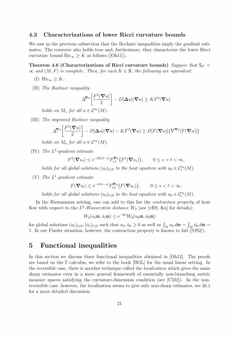
4.3 Characterizations of lower Ricci curvature bounds

We saw in the previous subsection that the Bochner inequalities imply the gradient esti-mates. The converse also holds true and, furthermore, they characterize the lower Riccicurvature bound Ric∞ ≥ K as follows ([Oh11]).

Theorem 4.6 (Characterizations of Ricci curvature bounds) Suppose that SF <∞ and (M,F ) is complete. Then, for each K ∈ R, the following are equivalent:

(I) Ric∞ ≥ K.

(II) The Bochner inequality

∆∇u

[F 2(∇u)

2

]−D[∆u](∇u) ≥ KF 2(∇u)

holds on Mu for all u ∈ C∞(M).

(III) The improved Bochner inequality

∆∇u

[F 2(∇u)

2

]−D[∆u](∇u)−KF 2(∇u) ≥ D[F (∇u)]

(∇∇u[F (∇u)]

)holds on Mu for all u ∈ C∞(M).

(IV) The L2-gradient estimate

F 2(∇ut) ≤ e−2K(t−s)P∇us,t

(F 2(∇us)

), 0 ≤ s < t <∞,

holds for all global solutions (ut)t≥0 to the heat equation with u0 ∈ C∞c (M).

(V) The L1-gradient estimate

F (∇ut) ≤ e−K(t−s)P∇us,t

(F (∇us)

), 0 ≤ s < t <∞,

holds for all global solutions (ut)t≥0 to the heat equation with u0 ∈ C∞c (M).

In the Riemannian setting, one can add to this list the contraction property of heatflow with respect to the L2-Wasserstein distance W2 (see [vRS, Ku] for details):

W2(utm, utm) ≤ e−KtW2(u0m, u0m)

for global solutions (ut)t≥0, (ut)t≥0 such that u0, u0 ≥ 0 as well as∫Mu0 dm =

∫Mu0 dm =

1. In our Finsler situation, however, the contraction property is known to fail ([OS2]).

5 Functional inequalities

In this section we discuss three functional inequalities obtained in [Oh12]. The proofsare based on the Γ-calculus, we refer to the book [BGL] for the usual linear setting. Inthe reversible case, there is another technique called the localization which gives the samesharp estimates even in a more general framework of essentially non-branching metricmeasure spaces satisfying the curvature-dimension condition (see [CM2]). In the non-reversible case, however, the localization seems to give only non-sharp estimates, see §6.1for a more detailed discussion.

21

5.1 Poincare–Lichnerowicz inequality

We start with the Poincare–Lichnerowicz (spectral gap) inequality under the curvaturebound RicN ≥ K > 0. The N ∈ [n,∞] case was shown in [Oh3] as a consequence ofthe curvature-dimension condition CD(K,N). In the Riemannian setting, the case ofN ∈ (−∞, 0) was shown independently in [KM] and [Oh9].

For simplicity we will assume that M is compact (this is automatically true whenN ∈ [n,∞) and M is complete), and normalize m as m(M) = 1. We will give the proofssince they are not long.

Proposition 5.1 Assume that M is compact and satisfies RicN ≥ K for some K ∈ Rand N ∈ (−∞, 0) ∪ [n,∞]. Then we have, for any f ∈ H2(M) ∩ C1(M) such that∆f ∈ H1(M), ∫

M

{D[∆f ](∇f) +KF 2(∇f) +

(∆f)2

N

}dm ≤ 0.

In particular, if K > 0, then we have∫M

F 2(∇f) dm ≤ N − 1

KN

∫M

(∆f)2 dm. (5.1)

If N =∞, then the coefficient in the RHS of (5.1) is read as 1/K.

Proof. The first assertion is a direct consequence of Theorem 3.5 with ϕ ≡ 1. We furtherobserve, by the integration by parts,

K

∫M

F 2(∇f) dm+∥∆f∥2L2

N≤ −

∫M

D[∆f ](∇f) dm = ∥∆f∥2L2 .

Rearranging this inequality yields (5.1) when K > 0. 2

Now the Poincare–Lichnerowicz inequality is obtained by a technique somewhat re-lated to the proof of Theorem 4.3. We define the variance of f ∈ L2(M) (underm(M) = 1)as

Varm(f) :=

∫M

f 2 dm−(∫

M

f dm

)2

.

Theorem 5.2 (Poincare–Lichnerowicz inequality) Let M be compact, m(M) = 1,and suppose RicN ≥ K > 0 for some N ∈ (−∞, 0) ∪ [n,∞]. Then we have, for anyf ∈ H1(M),

Varm(f) ≤N − 1

KN

∫M

F 2(∇f) dm.

Proof. Let (ut)t≥0 be the solution to the heat equation with u0 = f , and put Φ(t) :=∥ut∥2L2 for t ≥ 0. Observe first that the ergodicity

ut →∫M

u0 dm in L2(M) (5.2)

22

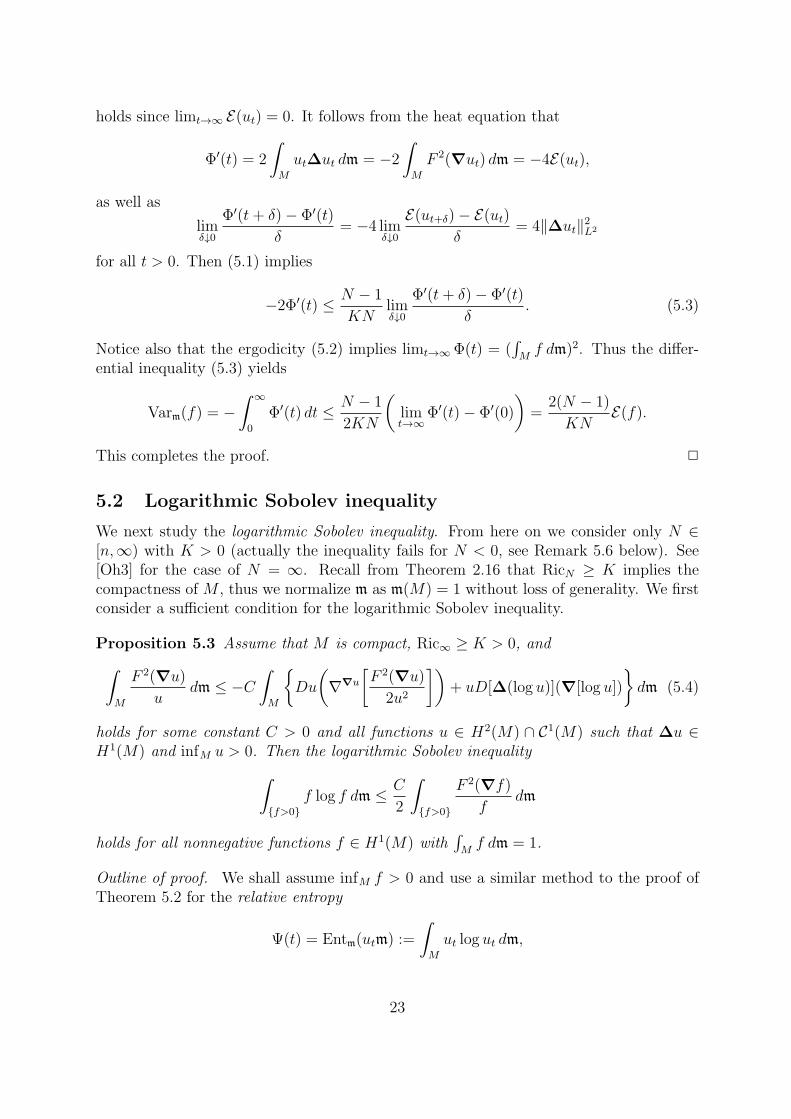
holds since limt→∞ E(ut) = 0. It follows from the heat equation that

Φ′(t) = 2

∫M

ut∆ut dm = −2∫M

F 2(∇ut) dm = −4E(ut),

as well as

limδ↓0

Φ′(t+ δ)− Φ′(t)

δ= −4 lim

δ↓0

E(ut+δ)− E(ut)δ

= 4∥∆ut∥2L2

for all t > 0. Then (5.1) implies

−2Φ′(t) ≤ N − 1

KNlimδ↓0

Φ′(t+ δ)− Φ′(t)

δ. (5.3)

Notice also that the ergodicity (5.2) implies limt→∞ Φ(t) = (∫Mf dm)2. Thus the differ-

ential inequality (5.3) yields

Varm(f) = −∫ ∞

0

Φ′(t) dt ≤ N − 1

2KN

(limt→∞

Φ′(t)− Φ′(0)

)=

2(N − 1)

KNE(f).

This completes the proof. 2

5.2 Logarithmic Sobolev inequality

We next study the logarithmic Sobolev inequality. From here on we consider only N ∈[n,∞) with K > 0 (actually the inequality fails for N < 0, see Remark 5.6 below). See[Oh3] for the case of N = ∞. Recall from Theorem 2.16 that RicN ≥ K implies thecompactness of M , thus we normalize m as m(M) = 1 without loss of generality. We firstconsider a sufficient condition for the logarithmic Sobolev inequality.

Proposition 5.3 Assume that M is compact, Ric∞ ≥ K > 0, and∫M

F 2(∇u)

udm ≤ −C

∫M

{Du

(∇∇u

[F 2(∇u)

2u2

])+ uD[∆(log u)](∇[log u])

}dm (5.4)

holds for some constant C > 0 and all functions u ∈ H2(M) ∩ C1(M) such that ∆u ∈H1(M) and infM u > 0. Then the logarithmic Sobolev inequality∫

{f>0}f log f dm ≤ C

2

∫{f>0}

F 2(∇f)

fdm

holds for all nonnegative functions f ∈ H1(M) with∫Mf dm = 1.

Outline of proof. We shall assume infM f > 0 and use a similar method to the proof ofTheorem 5.2 for the relative entropy

Ψ(t) = Entm(utm) :=

∫M

ut log ut dm,

23

where (ut)t≥0 is the solution to the heat equation with u0 = f . The inequality (5.4)then yields the differential inequality −2Ψ′(t) ≤ CΨ′′(t). Together with limt→∞ Ψ(t) =limt→∞Ψ′(t) = 0, we obtain∫

M

f log f dm = −∫ ∞

0

Ψ′(t) dt ≤ C

2

∫ ∞

0

Ψ′′(t) dt = −C2Ψ′(0).

This is indeed the desired inequality. 2

See [Oh12] and [BGL] for the omitted calculations in the proofs of the propositionabove and the theorem below.

Theorem 5.4 (Logarithmic Sobolev inequality) Assume that RicN ≥ K > 0 forsome N ∈ [n,∞) and m(M) = 1. Then we have∫

{f>0}f log f dm ≤ N − 1

2KN

∫{f>0}

F 2(∇f)

fdm

for all nonnegative functions f ∈ H1(M) with∫Mf dm = 1.

Outline of proof. Fix h ∈ C∞(M) and consider the function eah for a > 0 (chosen later).For brevity let us introduce the notation common in the Γ-calculus:

Γ2(h) := ∆∇h

[F 2(∇h)

2

]−D[∆h](∇h).

On the one hand, by the chain rule and a > 0, we calculate

Γ2(eah) = a2e2ah

{Γ2(h) + aD[F 2(∇h)](∇h) + a2F 4(∇h)

}(notice that a > 0 yields ∇(eah) = aeah∇h). On the other hand, it follows from theintegration by parts that∫

M

Γ2(eah) dm = a2

∫M

e2ah{(∆h)2 − 2aD[F 2(∇h)](∇h)− 3a2F 4(∇h)

}dm.

Comparing these yields∫M

e2ah(∆h)2 dm =

∫M

e2ah{Γ2(h) + 3aD[F 2(∇h)](∇h) + 4a2F 4(∇h)

}dm. (5.5)

We apply the Bochner inequality (3.3) to eah, now written as Γ2(eah) ≥ KF 2(∇eah)+

(∆eah)2/N , and see

Γ2(h) + aD[F 2(∇h)](∇h) + a2F 4(∇h)

≥ KF 2(∇h) +1

N

{(∆h)2 + 2aF 2(∇h)∆h+ a2F 4(∇h)

}(5.6)

24

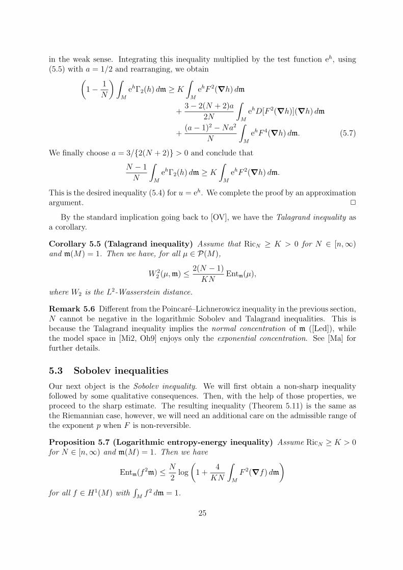
in the weak sense. Integrating this inequality multiplied by the test function eh, using(5.5) with a = 1/2 and rearranging, we obtain(

1− 1

N

)∫M

ehΓ2(h) dm ≥ K

∫M

ehF 2(∇h) dm

+3− 2(N + 2)a

2N

∫M

ehD[F 2(∇h)](∇h) dm

+(a− 1)2 −Na2

N

∫M

ehF 4(∇h) dm. (5.7)

We finally choose a = 3/{2(N + 2)} > 0 and conclude that

N − 1

N

∫M

ehΓ2(h) dm ≥ K

∫M

ehF 2(∇h) dm.

This is the desired inequality (5.4) for u = eh. We complete the proof by an approximationargument. 2

By the standard implication going back to [OV], we have the Talagrand inequality asa corollary.

Corollary 5.5 (Talagrand inequality) Assume that RicN ≥ K > 0 for N ∈ [n,∞)and m(M) = 1. Then we have, for all µ ∈ P(M),

W 22 (µ,m) ≤ 2(N − 1)

KNEntm(µ),

where W2 is the L2-Wasserstein distance.

Remark 5.6 Different from the Poincare–Lichnerowicz inequality in the previous section,N cannot be negative in the logarithmic Sobolev and Talagrand inequalities. This isbecause the Talagrand inequality implies the normal concentration of m ([Led]), whilethe model space in [Mi2, Oh9] enjoys only the exponential concentration. See [Ma] forfurther details.

5.3 Sobolev inequalities

Our next object is the Sobolev inequality. We will first obtain a non-sharp inequalityfollowed by some qualitative consequences. Then, with the help of those properties, weproceed to the sharp estimate. The resulting inequality (Theorem 5.11) is the same asthe Riemannian case, however, we will need an additional care on the admissible range ofthe exponent p when F is non-reversible.

Proposition 5.7 (Logarithmic entropy-energy inequality) Assume RicN ≥ K > 0for N ∈ [n,∞) and m(M) = 1. Then we have

Entm(f2m) ≤ N

2log

(1 +

4

KN

∫M

F 2(∇f) dm

)for all f ∈ H1(M) with

∫Mf 2 dm = 1.

25

Outline of proof. It suffices to consider the case where c ≤ f ≤ C for some 0 < c <C < ∞. Let (ut)t≥0 be the solution to the heat equation with u0 = f 2, and put Ψ(t) :=Entm(utm) similarly to Proposition 5.3. By the Bochner inequality (3.3) and the Cauchy–Schwarz inequality we find

Ψ′′(t) ≥ −2KΨ′(t) +2

NΨ′(t)2.

This implies that the function

t 7−→ e−2Kt

(1

N− K

Ψ′(t)

)is non-decreasing in t > 0, and hence

−Ψ′(t) ≤ KN

{e2Kt

(1− KN

Ψ′(0)

)− 1

}−1

.

Integrating this inequality gives

Ψ(0)−Ψ(t) ≤ N

2log

(1− (1− e−2Kt)

Ψ′(0)

KN

).

Since

Ψ′(0) = −∫M

F 2(∇(f 2))

f 2dm = −4

∫M

F 2(∇f) dm,

letting t→∞ completes the proof. 2

The above inequality yields the Nash inequality and then a non-sharp Sobolev inequal-ity.

Lemma 5.8 (Nash inequality) Assume that RicN ≥ K > 0 for N ∈ [n,∞) andm(M) = 1. Then we have, for all f ∈ H1(M),

∥f∥N+2L2 ≤

(∥f∥2L2 +

4

KNE(f)

)N/2

∥f∥2L1 .

Outline of proof. Normalize f so as to satisfy∫Mf 2 dm = 1, and put ψ(θ) := log(∥f∥L1/θ)

for θ ∈ (0, 1]. We see by the Holder inequality that ψ is a convex function. Therefore

ψ(1) ≥ ψ

(1

2

)+

1

2ψ′(1

2

)=

1

2ψ′(1

2

)= −1

2Entm(f

2m).

Combining this with Proposition 5.7 gives the claim. 2

Proposition 5.9 (Non-sharp Sobolev inequality) Assume that RicN ≥ K > 0 forN ∈ [n,∞) ∩ (2,∞) and m(M) = 1. Then we have

∥f∥2Lp ≤ C1∥f∥2L2 + C2E(f)

for all f ∈ H1(M), where p = 2N/(N − 2), C1 = C1(N) > 1 and C2 = C2(K,N) > 0.

26

Outline of proof. We can assume c ≤ f ≤ C for some 0 < c < C <∞. Slice f into

fk(x) :=

2k if f(x) > 2k+1,

f − 2k if 2k < f(x) ≤ 2k+1,

0 if f(x) ≤ 2k,

for k ∈ Z. We show the claim by applying the Nash inequality to each fk. 2

The above Sobolev inequality has some applications those will be used to show thesharp inequality. Actually one can reduce such qualitative arguments to the Riemanniancase by observing the following.

Corollary 5.10 Assume that RicN ≥ K > 0 for N ∈ [n,∞) ∩ (2,∞) and m(M) = 1.Then there exists a C∞-Riemannian metric g for which

∥f∥2Lp ≤ C1∥f∥2L2 + C2SFEg(f)

holds for all f ∈ H1(M), where Eg is the energy form of (M, g,m) and p = 2N/(N − 2),C1 > 1 and C2 > 0 are as in Proposition 5.9.

We are now ready to show the sharp Sobolev inequality.

Theorem 5.11 (Sobolev inequality) Assume that RicN ≥ K > 0 for N ∈ [n,∞) andm(M) = 1. Then we have

∥f∥2Lp − ∥f∥2L2

p− 2≤ N − 1

KN

∫M

F 2(∇f) dm

for all 1 ≤ p ≤ 2(N + 1)/N and f ∈ H1(M).

The case of p = 2 is understood as the limit, giving the logarithmic Sobolev inequal-ity (Theorem 5.4). The p = 1 case amounts to the Poincare–Lichnerowicz inequality(Theorem 5.2).

Outline of proof. Take the smallest possible constant C > 0 satisfying

∥f∥2Lp − ∥f∥2L2

p− 2≤ 2CE(f) (5.8)

for all nonnegative functions f ∈ H1(M). In order to show C ≤ (N − 1)/KN , let ussuppose that there is an extremal (nonconstant) function f ≥ 0 enjoying equality in (5.8)as well as 0 < c ≤ f ≤ C < ∞. We normalize f as ∥f∥Lp = 1. The equality in (5.8)implies

f p−1 − f = −C(p− 2)∆f,

which improves the regularity of f . Put u := log f .

27

On the one hand, for b ≥ 0, it follows from (5.5) (with a = b/2) and the integrationby parts that

C

∫M

ebuΓ2(u) dm =

∫M

ebuF 2(∇u) dm

+ C

(p− 1− b

2

)∫M

ebuD[F 2(∇u)](∇u) dm

+ C(p− 2)(b− 1)

∫M

ebuF 4(∇u) dm. (5.9)

We remark that b ≥ 0 was required to apply (5.5). On the other hand, we deduce from(5.6) that(

1− 1

N

)∫M

ebuΓ2(u) dm ≥ K

∫M

ebuF 2(∇u) dm

+

(3b− 4a

2N− a

)∫M

ebuD[F 2(∇u)](∇u) dm

+

((a− b)2

N− a2

)∫M

ebuF 4(∇u) dm, (5.10)

which can be seen as a variant of (5.7). Comparing (5.9) and (5.10), we would like tochoose a and b enjoying

p− 1− b

2=

3b− 2(N + 2)a

2(N − 1), (p− 2)(b− 1) =

(a− b)2 −Na2

N − 1

as well as a ≥ 0, b ≥ 0. This is possible for p ∈ [1, 2(N + 1)/N ], and then we concludeC ≤ (N − 1)/KN as desired.

There remains the delicate issue that such an extremal function f does not necessarilyexist. Hence one needs an extra discussion on the approximation. This technical argumentcan be reduced to the Riemannian case thanks to the non-sharp Sobolev inequality inCorollary 5.10. See [BGL, Theorem 6.8.3] for details. 2

Remark 5.12 The admissible range of the exponent p is [1, 2N/(N − 2)] in the Rieman-nian and the reversible Finsler cases. In the above non-reversible situation, the additionalconstraints a ≥ 0 and b ≥ 0 make the range narrower. One can slightly extend the range[1, 2(N + 1)/N ] in Theorem 5.11 by a careful calculation into[

1,7N2 + 2N + (N + 2)

√N2 + 8N

4N(N − 1)

],

though it is still smaller than [1, 2N/(N − 2)].

6 Gaussian isoperimetric inequality

This final section is devoted to a geometric application of the Γ-calculus, the Gaussianisoperimetric inequality obtained in [Oh11]. This is the infinite dimensional counterpart

28

to the Levy–Gromov isoperimetric inequality, and was first established in the Riemanniansetting by Bakry–Ledoux [BL]. We will give historical background in §6.1 and the outlineof the proof in §6.2.

6.1 Background for Levy–Gromov isoperimetic inequality

Given a Finsler manifold (M,F,m) such that m(M) = 1, we define the isoperimetricprofile I(M,F,m) : [0, 1] −→ [0,∞] by

I(M,F,m)(θ) := inf{m+(A) |A ⊂M : Borel set with m(A) = θ},

where

m+(A) := lim infε↓0

m(B+(A, ε))−m(A)

ε, B+(A, ε) := {y ∈M | inf

x∈Ad(x, y) < ε}.

In the Riemannian case, the classical theorem of Levy and Gromov [Le1, Le2, Gr] assertsthat, for an n-dimensional Riemannian manifold (M, g) of Ric ≥ n−1 with the normalizedvolume measure m := volg(M)−1 volg, the isoperimetric profile I(M,g,m) is bounded frombelow by the profile of the unit sphere Sn:

I(M,g,mg)(θ) ≥ I(Sn,mSn )(θ), (6.1)

where mSn is the normalized volume measure as well. The standard strategy of the proofof (6.1) is as follows:

(1) We take an extremal region A ⊂M achieving the minimal boundary measure m+(A)with the prescribed volume θ.

(2) Then the deep theorem in geometric measure theory (a la Federer, Almgren et al)guarantees a certain regularity of the boundary of A.

(3) Perturbing A gives a differential inequality (a Heintze–Karcher type inequality).

(4) Combining the above differential inequality with the analysis of the behavior as θ ↓ 0gives the isoperimetic inequality.

Along the same strategy one can study the weighted version ([Bay]) and, moreover,the combinations of upper diameter bounds and lower curvature bounds ([Mi1]). Themost general work of Milman [Mi1] gave the sharp estimate:

I(M,g,m)(θ) ≥ IK,N,D(θ) (6.2)

for (M, g,m) with RicN ≥ K and diamM ≤ D, where IK,N,D is the explicit function.Up to now, however, the regularity theory is known only for Riemannian manifolds. Thishad been an obstacle for generalizations to Finsler manifolds as well as less smooth spacessuch as metric measure spaces.

In 2014, Klartag [Kl] gave a beautiful alternative proof of the Levy–Gromov isoperi-metric inequality, still on weighted Riemannian manifolds, but without the regularity

29

theory. His breakthrough was done by generalizing the localization method in convexgeometry to Riemannian manifolds with the help of optimal transport theory. The local-ization method, going back to [PW, GM, LS, KLS], is a sophisticated tool reducing aninequality to those on geodesics. Then the analysis becomes much simpler and clearer.

Inspired by [Kl], Cavalletti–Mondino generalized the localization method to essentiallynon-branching metric measure spaces satisfying the curvature-dimension condition, andshowed the isoperimetric inequality (6.2) in [CM1] and several functional inequalities in[CM2]. This class of spaces includes reversible Finsler manifolds. In [Oh10], we generalizedthe argument in [CM1] to possibly non-reversible Finsler manifolds, however, then itturned out that the localization method gives only a non-sharp estimate in the non-reversible case, precisely,

I(M,F,m)(θ) ≥ Λ−1F · IK,N,D(θ). (6.3)

This is due to the fact that reverse curves of geodesics are not necessarily geodesic. Itseems plausible to expect that Λ−1

F in (6.3) would be removed, that is to say, non-reversibleFinsler manifolds enjoy the same isoperimetric inequality as reversible Finsler manifolds.

Towards this direction, we consider the special case where N = D = ∞ and K > 0.This is the only case where we have another alternative proof of (6.1), based on the Γ-calculus ([BL]). As we saw in the previous section, the Γ-calculus is not sensitive to thenon-reversibility (only the exception was the range of p in Theorem 5.11), and we actuallyobtain the sharp estimate.

6.2 Isoperimetric inequality

In order to state the key estimate which is a kind of gradient estimate, we define

φ(c) :=1√2π

∫ c

−∞e−b2/2 db for c ∈ R, N (θ) := φ′ ◦ φ−1(θ) for θ ∈ (0, 1).

Set also N (0) = N (1) := 0.

Theorem 6.1 Assume Ric∞ ≥ K for some K ∈ R and SF <∞. Then we have, given aglobal solution (ut)t≥0 to the heat equation with u0 ∈ C∞c (M) and 0 ≤ u0 ≤ 1,√

N 2(ut) + αF 2(∇ut) ≤ P∇u0,t

(√N 2(u0) + cα(t)F 2(∇u0)

)(6.4)

for all α ≥ 0 and t > 0, where

cα(t) :=1− e−2Kt

K+ αe−2Kt > 0

and cα(t) := 2t+ α when K = 0.

For simplicity, we suppressed the dependence of cα on K.

Outline of proof. By the construction of global solutions as gradient curves, we find that0 ≤ u0 ≤ 1 implies 0 ≤ ut ≤ 1 for all t > 0, and hence N (ut) makes sense. Fix t > 0 andput

ζs :=√

N 2(us) + cα(t− s)F 2(∇us), 0 ≤ s ≤ t.

30

Then (6.4) is written as ζt ≤ P∇u0,t (ζ0), thereby we are done when we show ∂s[P

∇us,t (ζs)] ≤ 0.

We can see by a simple calculation that

∂s[P∇us,t (ζs)] = P∇u

s,t (∂sζs −∆∇usζs).

Hence it is sufficient to prove ∆∇usζs − ∂sζs ≥ 0 for 0 < s < t.By using c′α(t) = 2(1 −Kcα(t)), N ′′ = −1/N and the improved Bochner inequality

(Proposition 4.4), we obtain

∆∇usζs − ∂sζs ≥cα(t− s)N ′(us)

2

ζ3sF 4(∇us)

− cα(t− s)N (us)N ′(us)

ζ3sDus

(∇∇us [F 2(∇us)]

)+cα(t− s)

ζ3s

N 2(us)

F 2(∇us)D

[F 2(∇us)

2

](∇∇us

[F 2(∇us)

2

]).

Combining this with the Cauchy–Schwarz inequality

Dus(∇∇us [F 2(∇us)]

)≤ F (∇us)

√D[F 2(∇us)]

(∇∇us [F 2(∇us)]

)for g∇us , we conclude that

∆∇usζs − ∂sζs

≥ cα(t− s)ζ3s

(|N ′(us)|F 2(∇us)−

N (us)

2F (∇us)

√D[F 2(∇us)]

(∇∇us [F 2(∇us)]

))2

≥ 0.

This completes the proof. 2

If K > 0, then Ric∞ ≥ K implies m(M) < ∞ and hence we can normalize m (see[St1]). Choosing α = K−1 in (6.4) and letting t→∞ yields the following.

Corollary 6.2 Assume that (M,F ) is complete and satisfies Ric∞ ≥ K > 0, SF < ∞and m(M) = 1. Then we have, for any u ∈ C∞c (M) with 0 ≤ u ≤ 1,

√KN

(∫M

u dm

)≤

∫M

√KN 2(u) + F 2(∇u) dm. (6.5)

Now we are ready to show the isoperimetric inequality.

Theorem 6.3 (Gaussian isoperimetric inequality) Let (M,F,m) be complete andsatisfy Ric∞ ≥ K > 0, m(M) = 1 and SF <∞. Then we have

I(M,F,m)(θ) ≥ IK(θ) (6.6)

for all θ ∈ [0, 1], where

IK(θ) :=√K

2πe−Kc2(θ)/2 with θ =

∫ c(θ)

−∞

√K

2πe−Ka2/2 da.

31

Outline of proof. Let θ ∈ (0, 1). Fix a closed set A ⊂M with m(A) = θ and consider

uε(x) := max{1− ε−1d(x,A), 0}, ε > 0.

Notice that F (∇uε) = ε−1 on B−(A, ε) \ A, where

B−(A, ε) :={x ∈M

∣∣∣ infy∈A

d(x, y) < ε}.

Applying (6.5) to (smooth approximations of) uε and letting ε ↓ 0 implies, with the helpof N (0) = N (1) = 0,

√KN (θ) ≤ lim inf

ε↓0

m(B−(A, ε))−m(A)

ε.

This is the desired isoperimetric inequality for the reverse Finsler structure←−F (recall

Definition 2.4). Because the curvature bound Ric∞ ≥ K is common to F and←−F , we also

obtain (6.6). 2

The inequality (6.6) has the same form as the Riemannian case in [BL], thus it is sharpand a model space is the real line R equipped with the normal (Gaussian) distributiondm =

√K/2π e−Kx2/2 dx. See [BL] for the original work on general linear diffusion semi-

groups (influenced by Bobkov’s works [Bob1, Bob2]), [Bor, SC] for the classical Euclideanor Hilbert cases, and [AM] for the recent result on RCD(K,∞)-spaces.

References

[AT] J. C. Alvarez-Paiva and A. C. Thompson, Volumes in normed and Finsler spaces.A sampler of Riemann–Finsler geometry, 1–48, Math. Sci. Res. Inst. Publ., 50,Cambridge Univ. Press, Cambridge, 2004.

[AGS] L. Ambrosio, N. Gigli and G. Savare, Metric measure spaces with RiemannianRicci curvature bounded from below. Duke Math. J. 163 (2014), 1405–1490.

[AM] L. Ambrosio and A. Mondino, Gaussian-type isoperimetric inequalities inRCD(K,∞) probability spaces for positive K. Atti Accad. Naz. Lincei Rend.Lincei Mat. Appl. 27 (2016), 497–514.

[Au] L. Auslander, On curvature in Finsler geometry. Trans. Amer. Math. Soc. 79(1955), 378–388.

[Bak] D. Bakry, L’hypercontractivite et son utilisation en theorie des semigroupes.(French) Lectures on probability theory (Saint-Flour, 1992), 1–114, Lecture Notesin Math., 1581, Springer, Berlin, 1994.

[BE] D. Bakry and M. Emery, Diffusions hypercontractives. (French) Seminaire deprobabilites, XIX, 1983/84, 177–206, Lecture Notes in Math., 1123, Springer,Berlin, 1985.

32

[BGL] D. Bakry, I. Gentil and M. Ledoux, Analysis and geometry of Markov diffusionoperators. Springer, Cham, 2014.

[BL] D. Bakry and M. Ledoux, Levy–Gromov’s isoperimetric inequality for an infinite-dimensional diffusion generator. Invent. Math. 123 (1996), 259–281.

[BQ] D. Bakry and Z. Qian, Some new results on eigenvectors via dimension, diameter,and Ricci curvature. Adv. Math. 155 (2000), 98–153.

[BCL] K. Ball, E. A. Carlen and E. H. Lieb, Sharp uniform convexity and smoothnessinequalities for trace norms. Invent. Math. 115 (1994), 463–482.

[BCS] D. Bao, S.-S. Chern and Z. Shen, An introduction to Riemann-Finsler geometry.Springer-Verlag, New York, 2000.

[Bay] V. Bayle, Proprietes de concavite du profil isoperimetrique et applications(French). These de Doctorat, Institut Fourier, Universite Joseph-Fourier, Greno-ble, 2003.

[Bob1] S. Bobkov, A functional form of the isoperimetric inequality for the Gaussianmeasure. J. Funct. Anal. 135 (1996), 39–49.

[Bob2] S. G. Bobkov, An isoperimetric inequality on the discrete cube, and an elementaryproof of the isoperimetric inequality in Gauss space. Ann. Probab. 25 (1997), 206–214.

[Bor] C. Borell, The Brunn–Minkowski inequality in Gauss space. Invent. Math. 30(1975), 207–216.

[CM1] F. Cavalletti and A. Mondino, Sharp and rigid isoperimetric inequalities in metric-measure spaces with lower Ricci curvature bounds. Invent. Math. (to appear).Available at arXiv:1502.06465

[CM2] F. Cavalletti and A. Mondino, Sharp geometric and functional inequalities inmetric measure spaces with lower Ricci curvature bounds. Geom. Topol. 21 (2017),603–645.

[Ch+] B. Chow, S.-C. Chu, D. Glickenstein, C. Guenther, J. Isenberg, T. Ivey, D. Knopf,P. Lu, F. Luo, L. Ni, The Ricci flow: techniques and applications. Part I. Geo-metric aspects. American Mathematical Society, Providence, RI, 2007.

[EKS] M Erbar, K. Kuwada and K.-T. Sturm, On the equivalence of the entropiccurvature-dimension condition and Bochner’s inequality on metric measure spaces.Invent. Math. 201 (2015), 993–1071.

[Ev] L. C. Evans, Partial differential equations. American Mathematical Society, Prov-idence, RI, 1998.

33

[FLZ] F. Fang, X.-D. Li and Z. Zhang, Two generalizations of Cheeger-Gromoll split-ting theorem via Bakry–Emery Ricci curvature. Ann. Inst. Fourier (Grenoble) 59(2009), 563–573.

[GS] Y. Ge and Z. Shen, Eigenvalues and eigenfunctions of metric measure manifolds.Proc. London Math. Soc. (3) 82 (2001), 725–746.

[Gi1] N. Gigli, The splitting theorem in non-smooth context. Preprint (2013). Availableat arXiv:1302.5555

[Gi2] N. Gigli, Nonsmooth differential geometry – An approach tailored for spaces withRicci curvature bounded from below. Mem. Amer. Math. Soc. (to appear). Avail-able at arXiv:1407.0809

[Gr] M. Gromov, Metric structures for Riemannian and non-Riemannian spaces.Based on the 1981 French original. With appendices by M. Katz, P. Pansu andS. Semmes. Translated from the French by Sean Michael Bates. Birkhauser Boston,Inc., Boston, MA, 1999.

[GM] M. Gromov and V. D. Milman, Generalization of the spherical isoperimetric in-equality to uniformly convex Banach spaces. Compositio Math. 62 (1987), 263–282.

[KLS] R. Kannan, L. Lovasz and M. Simonovits, Isoperimetric problems for convexbodies and a localization lemma. Discrete Comput. Geom. 13 (1995), 541–559.

[Kl] B. Klartag, Needle decompositions in Riemannian geometry. Mem. Amer. Math.Soc. (to appear). Available at arXiv:1408.6322

[KM] A. V. Kolesnikov and E. Milman, Poincare and Brunn–Minkowski inequalitieson weighted Riemannian manifolds with boundary. Preprint (2013). Available atarXiv:1310.2526

[Ku] K. Kuwada, Duality on gradient estimates and Wasserstein controls. J. Funct.Anal. 258 (2010), 3758–3774.

[Led] M. Ledoux, The concentration of measure phenomenon. Mathematical Surveysand Monographs, 89. American Mathematical Society, Providence, RI, 2001.

[Lee] P. W. Y. Lee, Displacement interpolations from a Hamiltonian point of view. J.Funct. Anal. 265 (2013), 3163–3203.

[Le1] P. Levy, Lecons d’analyse fonctionnelle. Gauthier-Villars, Paris, 1922.

[Le2] P. Levy, Problemes concrets d’analyse fonctionnelle. Avec un complement surles fonctionnelles analytiques par F. Pellegrino (French). 2d ed. Gauthier-Villars,Paris, 1951.

[Li] A. Lichnerowicz, Varietes riemanniennes a tenseur C non negatif (French). C. R.Acad. Sci. Paris Ser. A-B 271 (1970), A650–A653.

34

[LV] J. Lott and C. Villani, Ricci curvature for metric-measure spaces via optimaltransport. Ann. of Math. 169 (2009), 903–991.

[LS] L. Lovasz and M. Simonovits, Random walks in a convex body and an improvedvolume algorithm. Random Structures Algorithms 4 (1993), 359–412.

[Ma] C. H. Mai, On Riemannian manifolds with positive weighted Ricci curvature ofnegative effective dimension. In preparation (2017).

[Mi1] E. Milman, Sharp isoperimetric inequalities and model spaces for curvature-dimension-diameter condition. J. Eur. Math. Soc. (JEMS) 17 (2015), 1041–1078.

[Mi2] E. Milman, Beyond traditional curvature-dimension I: new model spaces forisoperimetric and concentration inequalities in negative dimension. Trans. Amer.Math. Soc. 369 (2017), 3605–3637.

[Mi3] E. Milman, Harmonic measures on the sphere via curvature-dimension. Ann. Fac.Sci. Toulouse Math. (to appear). Available at arXiv:1505.04335

[MN] A. Mondino and A. Naber, Structure theory of metric-measure spaces with lowerRicci curvature bounds I. Preprint (2014). Available at arXiv:1405.2222

[Oh1] S. Ohta, On the measure contraction property of metric measure spaces. Com-ment. Math. Helv. 82 (2007), 805–828.

[Oh2] S. Ohta, Uniform convexity and smoothness, and their applications in Finslergeometry. Math. Ann. 343 (2009), 669–699.

[Oh3] S. Ohta, Finsler interpolation inequalities. Calc. Var. Partial Differential Equa-tions 36 (2009), 211–249.

[Oh4] S. Ohta, Optimal transport and Ricci curvature in Finsler geometry. Probabilisticapproach to geometry, 323–342, Adv. Stud. Pure Math., 57, Math. Soc. Japan,Tokyo, 2010.

[Oh5] S. Ohta, Vanishing S-curvature of Randers spaces. Differential Geom. Appl. 29(2011), 174–178.

[Oh6] S. Ohta, Ricci curvature, entropy, and optimal transport. Optimal transportation,145–199, London Math. Soc. Lecture Note Ser., 413, Cambridge Univ. Press,Cambridge, 2014.

[Oh7] S. Ohta, On the curvature and heat flow on Hamiltonian systems. Anal. Geom.Metr. Spaces 2 (2014), 81–114.

[Oh8] S. Ohta, Splitting theorems for Finsler manifolds of nonnegative Ricci curvature.J. Reine Angew. Math. 700 (2015), 155–174.

[Oh9] S. Ohta, (K,N)-convexity and the curvature-dimension condition for negative N .J. Geom. Anal. 26 (2016), 2067–2096.

35

[Oh10] S. Ohta, Needle decompositions and isoperimetric inequalities in Finsler geometry.J. Math. Soc. Japan (to appear). Available at arXiv:1506.05876

[Oh11] S. Ohta, A semigroup approach to Finsler geometry: Bakry–Ledoux’s isoperimet-ric inequality. Preprint (2016). Available at arXiv:1602.00390

[Oh12] S. Ohta, Some functional inequalities on non-reversible Finsler manifolds. Proc.Indian Acad. Sci. Math. Sci. (to appear). Available at arXiv:1701.05704

[OP] S. Ohta and M. Palfia, Gradient flows and a Trotter–Kato formula of semi-convex functions on CAT(1)-spaces. Amer. J. Math. (to appear). Available atarXiv:1411.1461

[OS1] S. Ohta and K.-T. Sturm, Heat flow on Finsler manifolds. Comm. Pure Appl.Math. 62 (2009), 1386–1433.

[OS2] S. Ohta and K.-T. Sturm, Non-contraction of heat flow on Minkowski spaces.Arch. Ration. Mech. Anal. 204 (2012), 917–944.

[OS3] S. Ohta and K.-T. Sturm, Bochner–Weitzenbock formula and Li–Yau estimateson Finsler manifolds. Adv. Math. 252 (2014), 429–448.

[OV] F. Otto and C. Villani, Generalization of an inequality by Talagrand and linkswith the logarithmic Sobolev inequality. J. Funct. Anal. 173 (2000), 361–400.

[PW] L. E. Payne and H. F. Weinberger, An optimal Poincare inequality for convexdomains. Arch. Rational Mech. Anal. 5 (1960), 286–292.

[Qi] Z. Qian, Estimates for weighted volumes and applications. Quart. J. Math. OxfordSer. (2) 48 (1997), 235–242.

[vRS] M.-K. von Renesse and K.-T. Sturm, Transport inequalities, gradient estimates,entropy and Ricci curvature. Comm. Pure Appl. Math. 58 (2005), 923–940.

[Sal] L. Saloff-Coste, Uniformly elliptic operators on Riemannian manifolds. J. Differ-ential Geom. 36 (1992), 417–450.

[SS] Y.-B. Shen and Z. Shen, Introduction to modern Finsler geometry. World ScientificPublishing Co., Singapore, 2016.

[Sh1] Z. Shen, Volume comparison and its applications in Riemann-Finsler geometry.Adv. Math. 128 (1997), 306–328.

[Sh2] Z. Shen, Lectures on Finsler geometry. World Scientific Publishing Co., Singapore,2001.

[St1] K.-T. Sturm, On the geometry of metric measure spaces. I. Acta Math. 196(2006), 65–131.

[St2] K.-T. Sturm, On the geometry of metric measure spaces. II. Acta Math. 196(2006), 133–177.

36

[SC] V. N. Sudakov and B. S. Cirel’son, Extremal properties of half-spaces for spher-ically invariant measures. (Russian) Problems in the theory of probability distri-butions, II. Zap. Naucn. Sem. Leningrad. Otdel. Mat. Inst. Steklov. (LOMI) 41(1974), 14–24, 165.

[Vi] C. Villani, Optimal transport, old and new. Springer-Verlag, Berlin, 2009.

[WX] G. Wang and C. Xia, A sharp lower bound for the first eigenvalue on Finslermanifolds. Ann. Inst. H. Poincare Anal. Non Lineaire 30 (2013), 983–996.

[WW] G. Wei and W. Wylie, Comparison geometry for the Bakry–Emery Ricci tensor.J. Differential Geom. 83 (2009), 377–405.

[Wy] W. Wylie, A warped product version of the Cheeger–Gromoll splitting theorem.Trans. Amer. Math. Soc. (to appear). Available at arXiv:1506.03800

[Xi] C. Xia, Local gradient estimate for harmonic functions on Finsler manifolds. Calc.Var. Partial Differential Equations 51 (2014), 849–865.

[YH] S.-T. Yin and Q. He, The first eigenvalue of Finsler p-Laplacian. Differential Geom.Appl. 35 (2014), 30–49.

37