nonlinear dynamics - blog.espci.fr · a period-doubling bifurcation, and is a phenomenon that...
TRANSCRIPT
1 Discrete Dynamical Systems or Mappings
A discrete dynamical system is of the form
yn+1 = g(yn) (1)
wherey andg are real vectors of the same dimension. A fixed point of (1) is a solution to
y = g(y) (2)
In one dimension, linear stability analysis ofy is carried out by writing
yn = y + ǫn
yn+1 = g(yn)
y + ǫn+1 = g(y + ǫn)
= g(y) + g′(y)ǫn +1
2g′′(y)ǫ2n · · ·
ǫn+1 ≈ g′(y)ǫn (3)
We see that|ǫ| decreases, i.e.y is a stable fixed point, if|g′(y)| < 1 and that|ǫ| grows, i.e. y is anunstable fixed point, if|g′(y)| > 1. In a multidimensional system,g′(y) is replaced by the JacobianDg(y) andy is a stable fixed point if all of the eigenvaluesµ of Dg(y) satisfy|µ| < 1, i.e. are inside theunit circle.
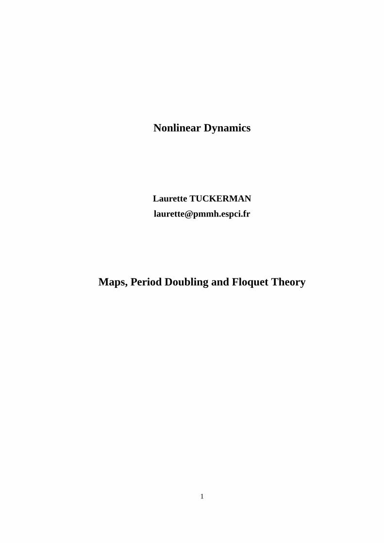
Loss of stability can take place in three different ways, as illustrated in figure1:
i) An eigenvalue may exit the unit circle at(1, 0).
ii) A complex conjugate pair of eigenvalues may exit the unit circle ate±iθ.
iii) An eigenvalue may exit the unit circle at(−1, 0).
Figure 1: Eigenvalues (or complex conjugate pairs of eigenvalues) can exit the unit circle in three ways:at (1,0), ate±iθ or at (-1,0).
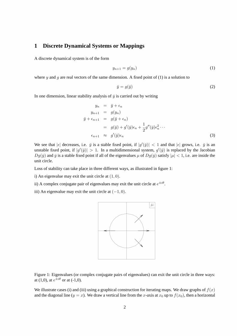
We illustrate cases (i) and (iii) using a graphical construction for iterating maps. We draw graphs off(x)and the diagonal line (y = x). We draw a vertical line from thex-axis atx0 up tof(x0), then a horizontal
2
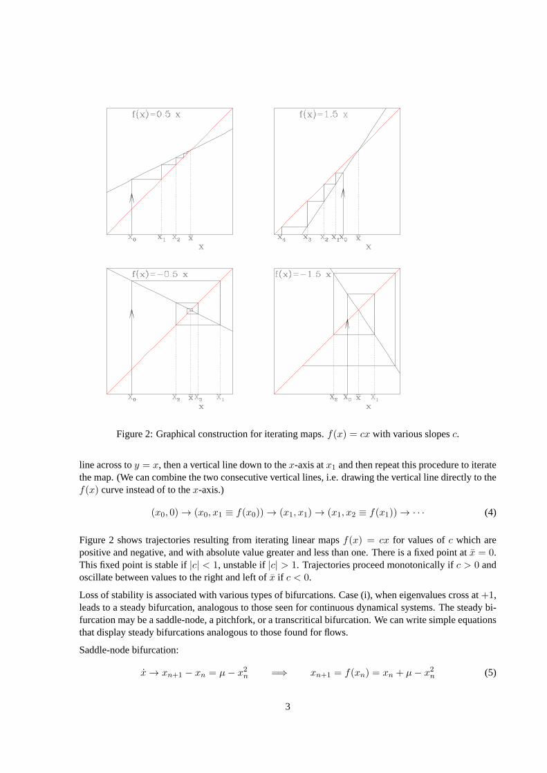
Figure 2: Graphical construction for iterating maps.f(x) = cx with various slopesc.
line across toy = x, then a vertical line down to thex-axis atx1 and then repeat this procedure to iteratethe map. (We can combine the two consecutive vertical lines, i.e. drawing the vertical line directly to thef(x) curve instead of to thex-axis.)
(x0, 0) → (x0, x1 ≡ f(x0)) → (x1, x1) → (x1, x2 ≡ f(x1)) → · · · (4)
Figure 2 shows trajectories resulting from iterating linear mapsf(x) = cx for values ofc which arepositive and negative, and with absolute value greater and less than one.There is a fixed point atx = 0.This fixed point is stable if|c| < 1, unstable if|c| > 1. Trajectories proceed monotonically ifc > 0 andoscillate between values to the right and left ofx if c < 0.
Loss of stability is associated with various types of bifurcations. Case (i), when eigenvalues cross at+1,leads to a steady bifurcation, analogous to those seen for continuous dynamical systems. The steady bi-furcation may be a saddle-node, a pitchfork, or a transcritical bifurcation. We can write simple equationsthat display steady bifurcations analogous to those found for flows.
Saddle-node bifurcation:
x → xn+1 − xn = µ− x2n =⇒ xn+1 = f(xn) = xn + µ− x2n (5)
3

Fixed points±√µ satisfyingf(x) = x exist forµ > 0. Their stability is calculated via
f(x) = x+ µ− x2
f ′(x) = 1− 2x (6)
f ′(±√µ) = 1∓ 2
√µ ≶ 1 for µ > 0
Pitchfork bifurcation:
x → xn+1 − xn = µxn − x3n =⇒ xn+1 = f(xn) = xn + µxn − x3n (7)
The fixed points0,±√µ satisfyf(x) = x. Their stability is calculated via
f(x) = x+ µx− x3
f ′(x) = 1 + µ− 2x2
f ′(0) = 1 + µ ≶ 1 for µ ≶ 0 (8)
f ′(±√µ) = 1− µ < 1 for µ > 0 (9)
Subcritical pitchfork bifurcations and transcritical bifurcations can alsooccur. Saddle-node and pitchfork(super and subcritical) bifurcations are illustrated in figure 3.
Case (ii), when eigenvalues cross ate±iθ, leads to a secondary Hopf, or Neimark-Sacker, bifurcation to atorus. We will discuss this in the next chapter. Case (iii), when eigenvaluescross at−1 leads to a flip, ora period-doubling bifurcation, and is a phenomenon that cannot occur for continuous dynamical systems.We now discuss this case in the context of the logistic map.
2 Logistic Map
The logistic map was proposed in the 1800s and popularized in the 1970s as amodel for populationbiology. Population growth is geometric (the next value is a multiple of the current value) when thepopulation is small, but is reduced when the population is too large. It is with this map that the famousperiod-doubling cascade was discovered, also in the 1970s, by Feigenbaum in Los Alamos, U.S. and,almost simultaneously, by Coullet and Tresser in Nice, France.
2.1 Fixed points and period doubling
The logistic map is defined by:
xn+1 = f(xn) ≡ axn(1− xn) for xn ∈ [0, 1], 0 < a < 4 (10)
f is a quadratic function mapping[0, 1] into itself, with minima at the two endpointsf(0) = f(1) = 0and a maximum at the midpointf(1/2) = a/4. Its fixed points are easily calculated:
x = ax(1− x) =⇒{
x = 0 or1 = a(1− x) =⇒ 1− x = 1/a =⇒ x = 1− 1/a
(11)
These are shown in figure 4.
4

Figure 3: Steady bifurcations for discrete dynamical systems.Top row: Saddle-node bifurcation.f(x) = x+ µ− x2 for µ = −0.2 (left) and forµ = 0.2 (middle).Middle row: Supercritical pitchfork.f(x) = x+ µx− x3 for µ = −0.2 (left) and forµ = 0.4 (middle).Bottom row: Subcritical pitchfork.f(x) = x+ µx+ x3 for µ = −0.4 (left) and forµ = 0.2 (middle).Right: corresponding bifurcation diagrams.
5
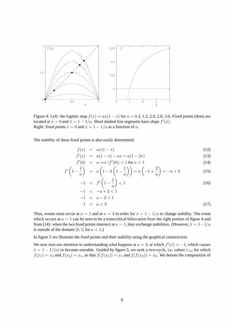
Figure 4: Left: the logistic mapf(x) = ax(1− x) for a = 0.4, 1.2, 2.0, 2.8, 3.6. Fixed points (dots) arelocated atx = 0 andx = 1− 1/a. Short dashed line segments have slopef ′(x).Right: fixed pointsx = 0 andx = 1− 1/a as a function ofa.
The stability of these fixed points is also easily determined:
f(x) = ax(1− x) (12)
f ′(x) = a(1− x)− ax = a(1− 2x) (13)
f ′(0) = a =⇒ |f ′(0)| < 1 for a < 1 (14)
f ′
(
1− 1
a
)
= a
(
1− 2
(
1− 1
a
))
= a
(
−1 +2
a
)
= −a+ 2 (15)
−1 < f ′
(
1− 1
a
)
< 1 (16)
−1 < −a+ 2 < 1
−1 < a− 2 < 1
1 < a < 3 (17)
Thus, events must occur ata = 1 and ata = 3 in order forx = 1 − 1/a to change stability. The eventwhich occurs ata = 1 can be seen to be a transcritical bifurcation from the right portion of figure 4 andfrom (14): when the two fixed points intersect ata = 1, they exchange stabilities. (However,x = 1−1/ais outside of the domain[0, 1] for a < 1.)
In figure 5 we illustrate the fixed points and their stability using the graphical construction.
We now turn our attention to understanding what happens ata = 3, at whichf ′(x) = −1, which causesx = 1 − 1/(a) to become unstable. Guided by figure 5, we seek a two-cycle, i.e. valuesx1,2 for whichf(x1) = x2 andf(x2) = x1, so thatf(f(x1)) = x1 andf(f(x2)) = x2. We denote the composition of
6
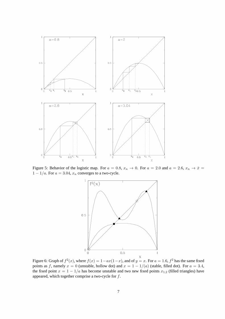
Figure 5: Behavior of the logistic map. Fora = 0.8, xn → 0. For a = 2.0 anda = 2.6, xn → x =1− 1/a. Fora = 3.04, xn converges to a two-cycle.
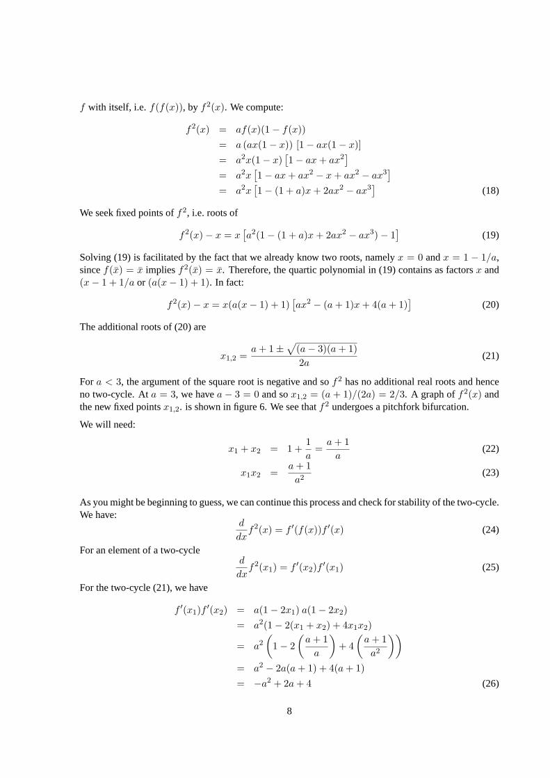
Figure 6: Graph off2(x), wheref(x) = 1−ax(1−x), and ofy = x. Fora = 1.6, f2 has the same fixedpoints asf , namelyx = 0 (unstable, hollow dot) andx = 1 − 1/(a) (stable, filled dot). Fora = 3.4,the fixed pointx = 1 − 1/a has become unstable and two new fixed pointsx1,2 (filled triangles) haveappeared, which together comprise a two-cycle forf .
7
f with itself, i.e.f(f(x)), by f2(x). We compute:
f2(x) = af(x)(1− f(x))
= a (ax(1− x)) [1− ax(1− x)]
= a2x(1− x)[
1− ax+ ax2]
= a2x[
1− ax+ ax2 − x+ ax2 − ax3]
= a2x[
1− (1 + a)x+ 2ax2 − ax3]
(18)
We seek fixed points off2, i.e. roots of
f2(x)− x = x[
a2(1− (1 + a)x+ 2ax2 − ax3)− 1]
(19)
Solving (19) is facilitated by the fact that we already know two roots, namelyx = 0 andx = 1 − 1/a,sincef(x) = x impliesf2(x) = x. Therefore, the quartic polynomial in (19) contains as factorsx and(x− 1 + 1/a or (a(x− 1) + 1). In fact:
f2(x)− x = x(a(x− 1) + 1)[
ax2 − (a+ 1)x+ 4(a+ 1)]
(20)
The additional roots of (20) are
x1,2 =a+ 1±
√
(a− 3)(a+ 1)
2a(21)
For a < 3, the argument of the square root is negative and sof2 has no additional real roots and henceno two-cycle. Ata = 3, we havea − 3 = 0 and sox1,2 = (a + 1)/(2a) = 2/3. A graph off2(x) andthe new fixed pointsx1,2. is shown in figure 6. We see thatf2 undergoes a pitchfork bifurcation.
We will need:
x1 + x2 = 1 +1
a=
a+ 1
a(22)
x1x2 =a+ 1
a2(23)
As you might be beginning to guess, we can continue this process and check for stability of the two-cycle.We have:
d
dxf2(x) = f ′(f(x))f ′(x) (24)
For an element of a two-cycled
dxf2(x1) = f ′(x2)f
′(x1) (25)
For the two-cycle (21), we have
f ′(x1)f′(x2) = a(1− 2x1) a(1− 2x2)
= a2(1− 2(x1 + x2) + 4x1x2)
= a2(
1− 2
(
a+ 1
a
)
+ 4
(
a+ 1
a2
))
= a2 − 2a(a+ 1) + 4(a+ 1)
= −a2 + 2a+ 4 (26)
8
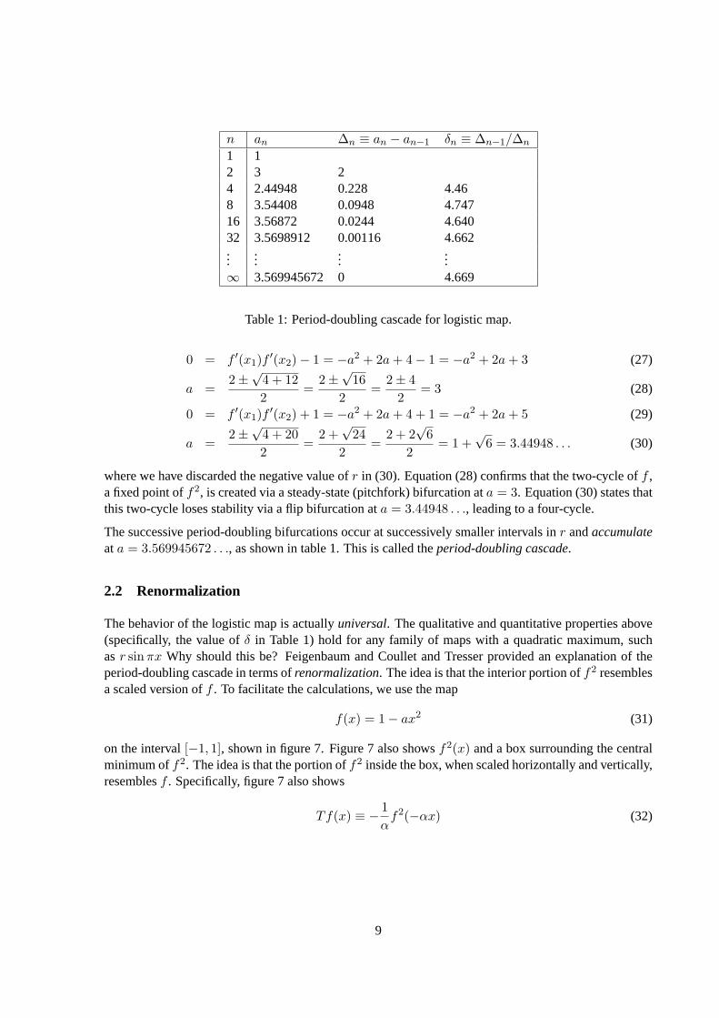
n an ∆n ≡ an − an−1 δn ≡ ∆n−1/∆n
1 12 3 24 2.44948 0.228 4.468 3.54408 0.0948 4.74716 3.56872 0.0244 4.64032 3.5698912 0.00116 4.662...
......
...∞ 3.569945672 0 4.669
Table 1: Period-doubling cascade for logistic map.
0 = f ′(x1)f′(x2)− 1 = −a2 + 2a+ 4− 1 = −a2 + 2a+ 3 (27)
a =2±
√4 + 12
2=
2±√16
2=
2± 4
2= 3 (28)
0 = f ′(x1)f′(x2) + 1 = −a2 + 2a+ 4 + 1 = −a2 + 2a+ 5 (29)
a =2±
√4 + 20
2=
2 +√24
2=
2 + 2√6
2= 1 +
√6 = 3.44948 . . . (30)
where we have discarded the negative value ofr in (30). Equation (28) confirms that the two-cycle off ,a fixed point off2, is created via a steady-state (pitchfork) bifurcation ata = 3. Equation (30) states thatthis two-cycle loses stability via a flip bifurcation ata = 3.44948 . . ., leading to a four-cycle.
The successive period-doubling bifurcations occur at successively smaller intervals inr andaccumulateata = 3.569945672 . . ., as shown in table 1. This is called theperiod-doubling cascade.
2.2 Renormalization
The behavior of the logistic map is actuallyuniversal. The qualitative and quantitative properties above(specifically, the value ofδ in Table 1) hold for any family of maps with a quadratic maximum, suchasr sinπx Why should this be? Feigenbaum and Coullet and Tresser provided an explanation of theperiod-doubling cascade in terms ofrenormalization. The idea is that the interior portion off2 resemblesa scaled version off . To facilitate the calculations, we use the map
f(x) = 1− ax2 (31)
on the interval[−1, 1], shown in figure 7. Figure 7 also showsf2(x) and a box surrounding the centralminimum off2. The idea is that the portion off2 inside the box, when scaled horizontally and vertically,resemblesf . Specifically, figure 7 also shows
Tf(x) ≡ − 1
αf2(−αx) (32)
9
The resemblance is quantified as follows:
f(x) ≈ Tf(x) (33)
1− ax2 ≈ − 1
αf2(−αx)
= − 1
αf(1− a(αx)2)
= − 1
α(1− a(1− a(αx)2)2)
= − 1
α(1− a(1− 2a(αx)2 + a2(αx)4))
= − 1
α(1− a+ 2a2(αx)2 − a3(αx)4) (34)
For the constant and quadratic terms in (34) to agree, we require
a− 1
α= 1
2a2α2
α= a
a− 1 = α 2aα = 1
2a(a− 1) = 1
α = 0.366 a =1 +
√3
2= 1.366 (35)
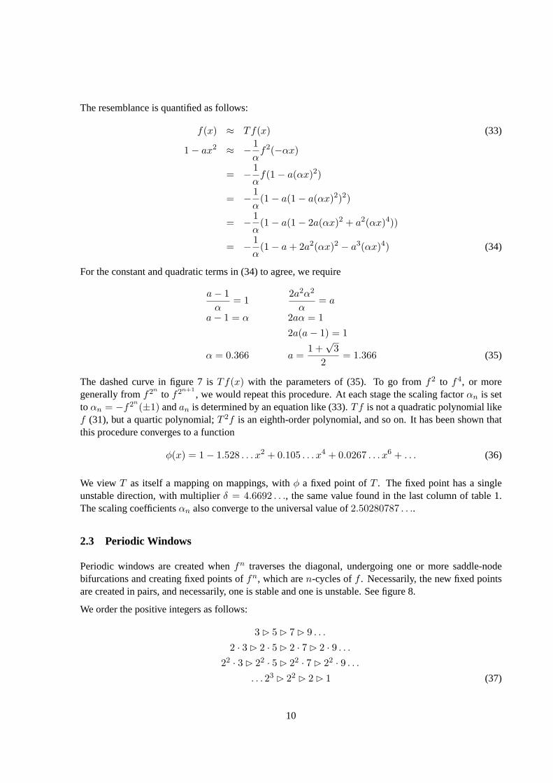
The dashed curve in figure 7 isTf(x) with the parameters of (35). To go fromf2 to f4, or moregenerally fromf2n to f2n+1
, we would repeat this procedure. At each stage the scaling factorαn is settoαn = −f2n(±1) andan is determined by an equation like (33).Tf is not a quadratic polynomial likef (31), but a quartic polynomial;T 2f is an eighth-order polynomial, and so on. It has been shown thatthis procedure converges to a function
φ(x) = 1− 1.528 . . . x2 + 0.105 . . . x4 + 0.0267 . . . x6 + . . . (36)
We viewT as itself a mapping on mappings, withφ a fixed point ofT . The fixed point has a singleunstable direction, with multiplierδ = 4.6692 . . ., the same value found in the last column of table 1.The scaling coefficientsαn also converge to the universal value of2.50280787 . . ..
2.3 Periodic Windows
Periodic windows are created whenfn traverses the diagonal, undergoing one or more saddle-nodebifurcations and creating fixed points offn, which aren-cycles off . Necessarily, the new fixed pointsare created in pairs, and necessarily, one is stable and one is unstable. See figure 8.
We order the positive integers as follows:
3⊲ 5⊲ 7⊲ 9 . . .
2 · 3⊲ 2 · 5⊲ 2 · 7⊲ 2 · 9 . . .22 · 3⊲ 22 · 5⊲ 22 · 7⊲ 22 · 9 . . .
. . . 23 ⊲ 22 ⊲ 2⊲ 1 (37)
10
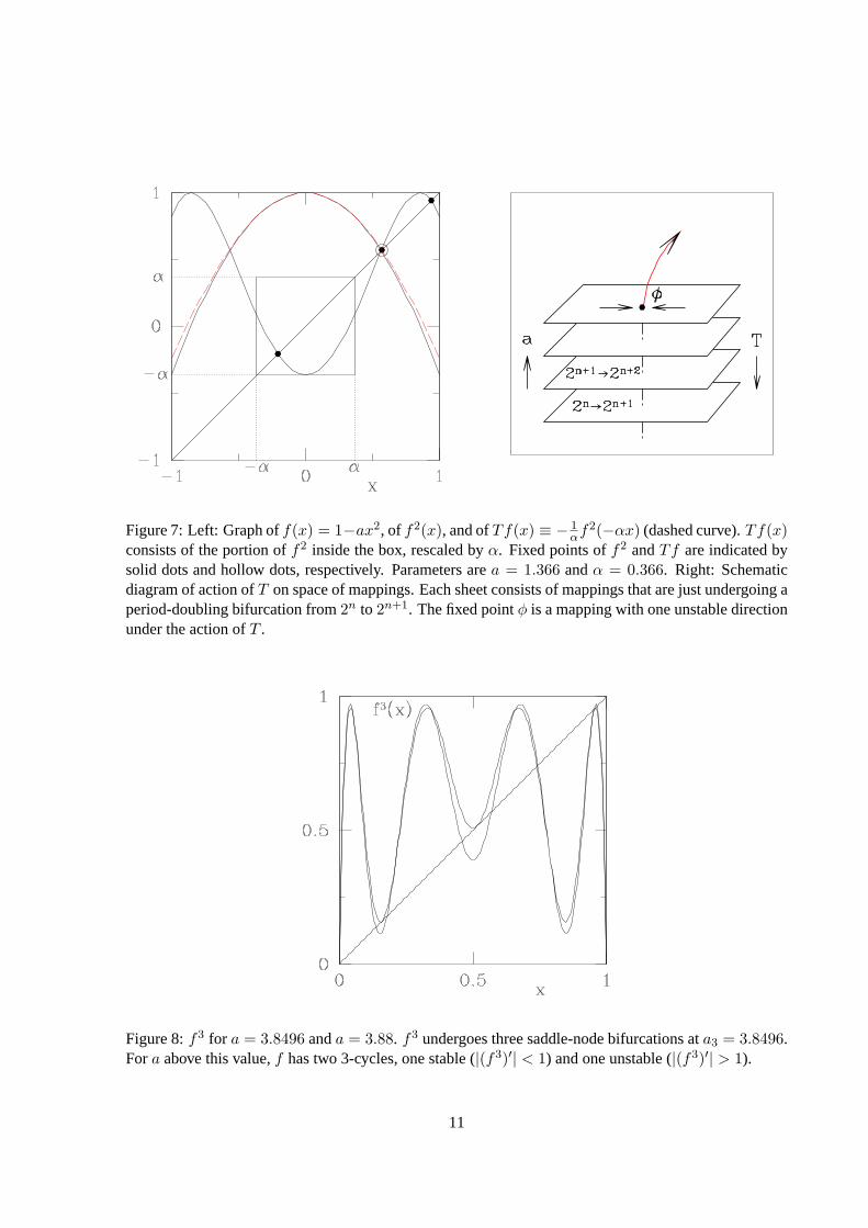
Figure 7: Left: Graph off(x) = 1−ax2, of f2(x), and ofTf(x) ≡ − 1αf2(−αx) (dashed curve).Tf(x)
consists of the portion off2 inside the box, rescaled byα. Fixed points off2 andTf are indicated bysolid dots and hollow dots, respectively. Parameters area = 1.366 andα = 0.366. Right: Schematicdiagram of action ofT on space of mappings. Each sheet consists of mappings that are just undergoing aperiod-doubling bifurcation from2n to 2n+1. The fixed pointφ is a mapping with one unstable directionunder the action ofT .
Figure 8:f3 for a = 3.8496 anda = 3.88. f3 undergoes three saddle-node bifurcations ata3 = 3.8496.Fora above this value,f has two 3-cycles, one stable (|(f3)′| < 1) and one unstable (|(f3)′| > 1).
11

Figure 9: Bifurcation diagram for logistic map, showing period-doubling cascade and periodic windows.Shown are fixed points or elements of cycles as a function ofr.
This is called the Sharkovskii order. Sharkovskii’s Theorem states thatif f has ak-cycle, then it anℓ-cycles for anyℓ ⊲ k. In particular, iff has a 3-cycle, then it has cycles of all lengths. This theoremsays nothing, in either the hypothesis or the conclusion, about the stability ofany of these cycles.
The logistic map has a 3-cycle, which originates in three simultaneous saddle-node bifurcations atr3 =(1 +
√8)/4 = 0.9624. This is illustrated in figure 8. Therefore, by Sharkovskii’s Theorem, thelogistic
map for anyr > r3 has cycles ofall lengths.
2.4 Tent Map and Shift Map
Other classes ofunimodal maps, characterized by the nature of their extrema, undergo a period-doublingcascade. Each class has its own asymptotic value ofδ andα. Examples are functions with a quarticmaximum and thetent map
f(x) =
{
2rx for x < 1/22r(1− x) for x > 1/2
(38)
shown in figure 10.
Consider the logistic mapping witha = 4
xn+1 = 4xn(1− xn) (39)
transformed to a new variable0 ≤ yn ≤ 1 via
xn = sin2(2πyn) (40)
12
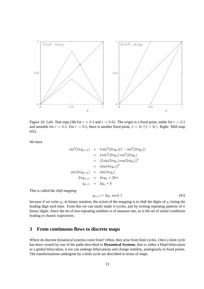
Figure 10: Left: Tent map (38) forr = 0.4 andr = 0.85. The origin is a fixed point, stable forr < 0.5and unstable forr > 0.5. Forr > 0.5, there is another fixed point,x = 2r/(1 + 2r). Right: Shift map(41).
We have
sin2(2πyn+1) = 4 sin2(2πyn)(1− sin2(2πyn))
= 4 sin2(2πyn) cos2(2πyn)
= (2 sin(2πyn) cos(2πyn))2
= (sin(4πyn))2
sin(2πyn+1) = sin(4πyn)
2πyn+1 = 4πyn + 2kπ
yn+1 = 2yn + k
This is called theshift mappingyn+1 = 2yn mod 1 (41)
because if we writeyn in binary notation, the action of the mapping is toshift the digits ofy, losing theleading digit each time. From this we can easily makek-cycles, just by writing repeating patterns ofkbinary digits. Since the set of non-repeating numbers is of measure one, so is the set of initial conditionsleading to chaotic trajectories.
3 From continuous flows to discrete maps
Where do discrete dynamical systems come from? Often, they arise from limit cycles. Once a limit cyclehas been created by one of the paths described inDynamical Systems, that is, either a Hopf bifurcationor a global bifurcation, it too can undergo bifurcations and change stability, analogously to fixed points.The transformations undergone by a limit cycle are described in terms of maps.
13

3.1 Floquet Theory
The linear stability of a limit cycle is described by the mathematical framework of Floquet theory. Alinear differential equation with constant coefficients such as
ax+ bx+ cx = 0 (42)
has as its general solutionx(t) = α1e
λ1t + α2eλ2t (43)
whereλ1,2 are the two solutions of the quadratic equation
aλ2 + bλ+ c = 0 (44)
The solutions of first andN th order linear differential equations are:
x = cx =⇒ x(t) = ectx(0) (45)N∑
n=0
cnx(n) = 0 =⇒ x(t) =
N∑
n=1
αneλnt (46)
wherex(n)(t) is thenth derivative ofx(t), {λn} are then roots of the equation
N∑
n=0
cnλn = 0 (47)
and the coefficientsαn are determined by the initial and/or boundary conditions.
This form can be generalized to equations in which the coefficients are notconstant, but periodic func-tions:
a(t)x+ b(t)x+ c(t)x = 0 (48)
a, b, c are all periodic functions with periodT . The general solution of (48), analogous to (43), is
x(t) = α1(t)eλ1t + α2(t)e
λ2t (49)
Functionsα1(t), α2(t) have the same period asa(t), b(t) andc(t) and are calledFloquet functions. Theexponentsλ1 andλ2 are calledFloquet exponents. In contrast to the exponents in (43), these are notroots of a polynomial and must be calculated numerically or asymptotically. The valuesµ1 ≡ eλ1T ,µ2 ≡ eλ2T are called Floquet multipliers.
Similarly, we have, for the first andN th order equations
x = c(t)x =⇒ x(t) = eλtα(t) (50)N∑
n=0
cn(t)x(n) = 0 =⇒ x(t) =
N∑
n=1
eλntαn(t) (51)
where theαn(t)’s have periodT .
We now consider a dynamical systemx = f(x) (52)
14

which has as its solution a limit cycle of periodT :
x(t+ T ) = x(t) (53)
that is,˙x(t) = f(x(t)) (54)
We now describe the evolution of a solution close to the limit cyclex:
x(t) = x(t) + ǫ(t) (55)
whereǫ(t) is assumed to remain small. Substituting (55) into (52), we obtain
˙x+ ǫ = f(x(t)) + f ′(x(t))ǫ(t) + f ′′(x(t))ǫ(t)2 + . . . (56)
Taking (54) into account and neglecting higher order terms leads to
ǫ = f ′(x(t))ǫ(t) (57)
which is of the Floquet form (50). Therefore:
ǫ(t) = eλtα(t) (58)
with α(t) periodic with periodT . The limit cyclex(t) is stable if the real part ofλ is negative. Ifλ iscomplex, this indicates that the period of the perturbationǫ is different from that of the limit cyclex(t).
For a multidimensional system of dimensionN , some of the equations above can be generalized to:
ǫ = Df(x(t))ǫ (59)
ǫ(t) =N∑
j=1
eλjtαj(t) (60)
There areN Floquet exponents and Floquet functions and the limit cyclex is stable if all the real partsof the exponents are negative. The Floquet multipliers and Floquet functions are eigenvalues and eigen-vectors of themonodromy matrixdefined as follows. LetM(t) be anN × N matrix whose evolutionequation and initial condition are:
M = Df(x(t))M M(0) = I (61)
M(T ) is the monodromy matrix. Thus, determining the Floquet exponents requires integrating theevolution equations linearized aboutx(t). The limit cyclex(t) is stable if all Floquet exponents havenegative real parts.
In order for the imaginary part to be unique, we chooseIm(λ) ∈ (−πi/T, πi/T ]. (The remainder canbe absorbed into the Floquet function.) See figure 11.
3.2 Poincare Mapping
Figure 12 presents schematic timeseries following a pitchfork and a period-doubling bifurcation in figure12.
15
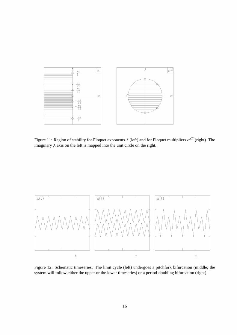
Figure 11: Region of stability for Floquet exponentsλ (left) and for Floquet multiplierseλT (right). Theimaginaryλ axis on the left is mapped into the unit circle on the right.
Figure 12: Schematic timeseries. The limit cycle (left) undergoes a pitchfork bifurcation (middle; thesystem will follow either the upper or the lower timeseries) or a period-doubling bifurcation (right).
16

Figure 13: First return, or Poincare mapping. Left: From P. Manneville, Class notes, DEA Physique desLiquides. Right: From Moehlis, Josic & Shea-Brown, Scholarpedia.
To better understand the flow in the vicinity of a limit cycle (or a more complicated attractor), we candefine a mapping, called the Poincare map or first return map, as follows. Lety ∈ Rd, and letyd be thelast component ofy (any other component could be chosen instead). Letβ be a value whichxd attainsduring the limit cycle. Letx ∈ R(d−1), containing all but thedth component ofx. We define:
xn+1 = g(xn) ⇐⇒
yd(t) = β, yd(t) > 0, y(t) = (xn, β)yd(t′) = β, yd(t′) > 0, y(t′) = (xn+1, β)yd(t′′) 6= β or yd(t′′) ≤ 0 for all t′′ ∈ (t, t′)
(62)
In order to avoid finding an appropriate valueβ, one can instead choose to select successive maxima ofone of the components, i.e.yd = 0.
This defines a discrete dynamical system, or mapping, forx ∈ Rd−1. The intersection of the trajectoryy(t) with the planeyd = β is mapped onto the next intersection (in the same direction). This constructionis illustrated in figure 13, where a flow (continuous dynamical system) ind dimensions is reduced to amap (discrete dynamical system) ind− 1 dimensions.
17

4 Examples from fluid dynamics
4.1 Faraday instability
Figure 14: Left: experimental setup for Faraday experiment. Right: quasicrystalline pattern of sur-face waves obtained by vertically oscillating a fluid layer with a two-frequency forcing function. FromEdwards & Fauve, J. Fluid Mech.279, 49 (1994).
In 1831, Faraday discovered that a pattern of standing waves was produced by vertical vibration of athin fluid layer as in the left portion of figure 14. Lattice patterns of hexagons, squares, and rolls havebeen observed and, more recently, in the 1990s, more exotic flows such as quasicrystalline patterns andoscillons. A picture of a quasicrystalline pattern can be seen in figure 14.
The imposed vibration can be considered as an oscillatory boundary condition, but it is simpler to go intoan oscillating frame of reference. The vibration then appears as an oscillatory gravitational forceG(t),which may be sinusoidal or more complicated:
G(t) = g (1− a cos(ωt)) (63)
G(t) = g (1− [a cos(mωt) + b cos(nωt+ φ0)]) (64)
We wish to determine when and to what the flat surface becomes linearly unstable. The domain can beconsidered to be homogeneous in the horizontal directions if these are sufficiently large. The linear insta-bility problem is therefore a constant-coefficient problem like (46) in the horizontal directions. Becausethe solutions must be bounded in the horizontal directions, the horizontal exponents are pure imaginary,i.e. the solutions are of the formexp(ik · x), or superpositions of these. Moreover, for a linear problem,solutions with different wavevectorsk are decoupled and can be considered separately, and each de-pends only onk = |k|. The vertical direction is neither homogeneous nor periodic, but can be eliminatedvia various manipulations. Therefore, the surface height variationζ corresponding to perturbations ofwavenumberk can be expanded as follows:
ζ(x, y, t) =∑
k
eik·xζk(t) (65)
On the other hand, because of the oscillating gravitational force (or boundary), the linear instability
18
problem is a Floquet problem like (51) in time and so solutionsζk(t) can be expanded
ζk(t) =∑
j
eλjktf j
k(t) (66)
where the functionsf jk(t) are periodic with periodT andλj
k are the Floquet exponents.
If the fluids are ideal (no viscosity) and the forcing is sinusoidal, then the height can be shown to begoverned by the classicMathieu equation:
∂ttζk + ω20 [1− a cos(ωt)] ζk = 0 (67)
whereω20 is a parameter combining the densities of the upper and lower fluids, the surface tension, the
wavenumberk and the gravitational accelerationg.
The Floquet multipliers areµjk ≡ eλ
jkT . If one of the|µj
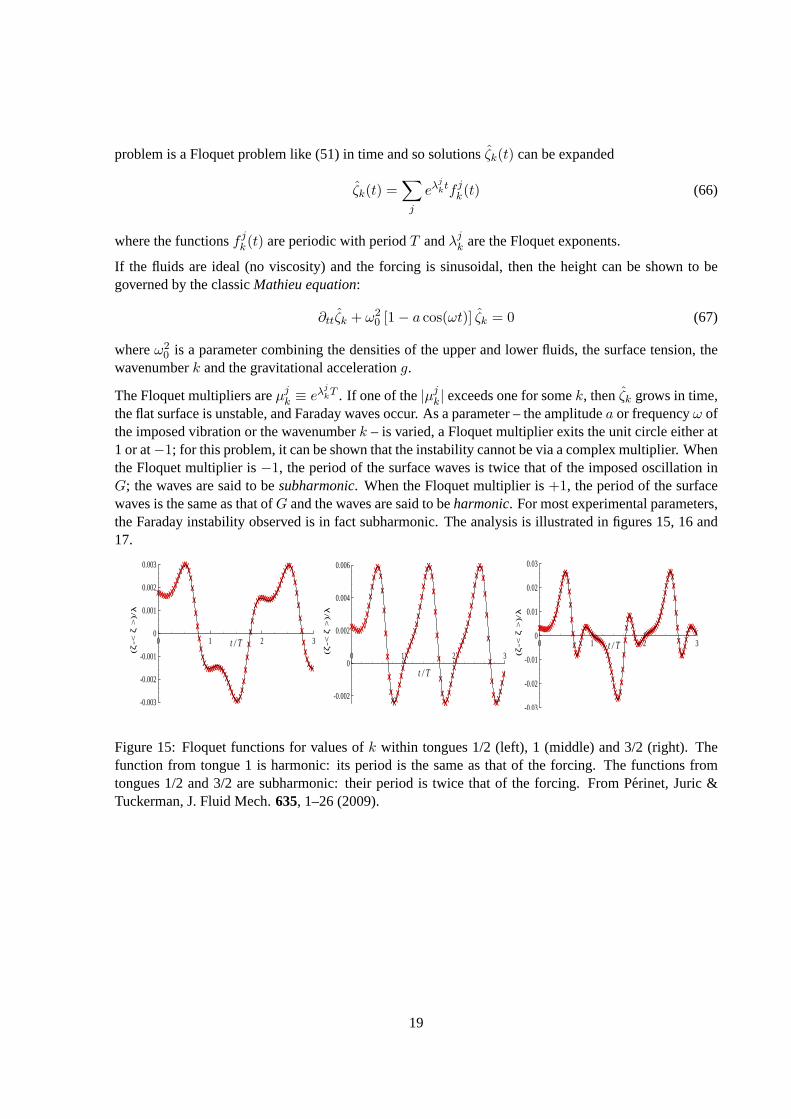
k| exceeds one for somek, thenζk grows in time,the flat surface is unstable, and Faraday waves occur. As a parameter– the amplitudea or frequencyω ofthe imposed vibration or the wavenumberk – is varied, a Floquet multiplier exits the unit circle either at1 or at−1; for this problem, it can be shown that the instability cannot be via a complex multiplier. Whenthe Floquet multiplier is−1, the period of the surface waves is twice that of the imposed oscillation inG; the waves are said to besubharmonic. When the Floquet multiplier is+1, the period of the surfacewaves is the same as that ofG and the waves are said to beharmonic. For most experimental parameters,the Faraday instability observed is in fact subharmonic. The analysis is illustrated in figures 15, 16 and17.
XXXXXXXXXXX
XXXX
XXXXXXX
X
X
XXXXXXXXXXXXXXXXXXXXXXXXX
XXX
X
X
XXXXX
XXXXXXXXXXXX
XXXX
XXXXXXX
X
X
XXXXXXX
t / T
(ζ-<
ζ>
)/
0 1 2 3
-0.003
-0.002
-0.001
0
0.001
0.002
0.003
λ
XXXXXXXXXXXXXXXXX
X
X
X
X
X
X
XXXX
XXXXXXXX
XXXXXXXXXXXX
X
X
X
X
X
X
XXXX
XXXXXXXX
XXXXXXXXXXXX
X
X
X
X
X
X
XXXX
XXXt / T
(ζ-<
ζ>
)/
0 1 2 3
-0.002
0
0.002
0.004
0.006
λ
XXXXXXXXXXXXXXXXXXXXXXXXX
X
X
XXXXX
XXXXXXXXXXXXXXXXXXXXXXXX
XXXXXXXXX
XX
X
X
X
XXXXX
XXXXXXXXX
XXXXXXXXX
XXXXXXXXXXXXXXX
X
X
X
X
XXXXX
XXXXXXXXXX
t / T
(ζ-<
ζ>
)/
0 1 2 3
-0.03
-0.02
-0.01
0
0.01
0.02
0.03
λ
Figure 15: Floquet functions for values ofk within tongues 1/2 (left), 1 (middle) and 3/2 (right). Thefunction from tongue 1 is harmonic: its period is the same as that of the forcing. The functions fromtongues 1/2 and 3/2 are subharmonic: their period is twice that of the forcing. From Perinet, Juric &Tuckerman, J. Fluid Mech.635, 1–26 (2009).
19
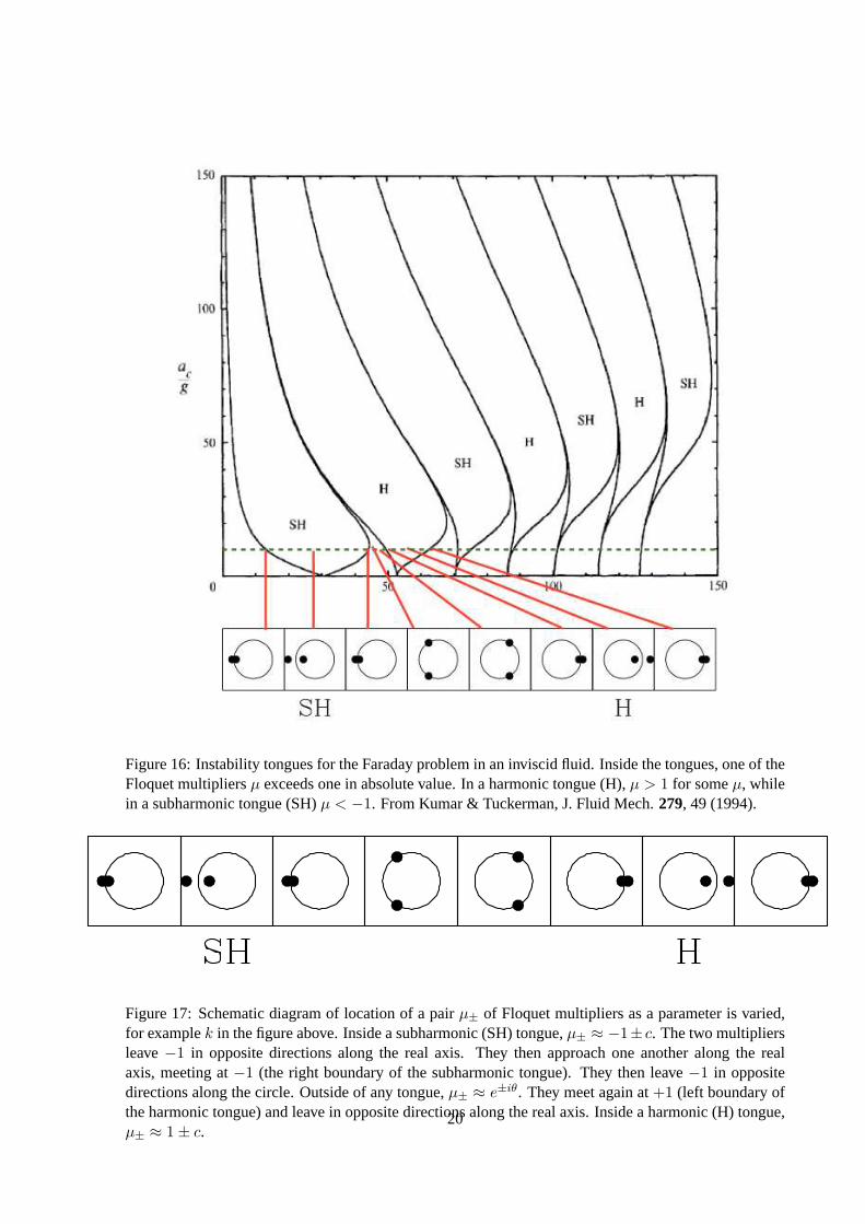
Figure 16: Instability tongues for the Faraday problem in an inviscid fluid. Inside the tongues, one of theFloquet multipliersµ exceeds one in absolute value. In a harmonic tongue (H),µ > 1 for someµ, whilein a subharmonic tongue (SH)µ < −1. From Kumar & Tuckerman, J. Fluid Mech.279, 49 (1994).
Figure 17: Schematic diagram of location of a pairµ± of Floquet multipliers as a parameter is varied,for examplek in the figure above. Inside a subharmonic (SH) tongue,µ± ≈ −1± c. The two multipliersleave−1 in opposite directions along the real axis. They then approach one another along the realaxis, meeting at−1 (the right boundary of the subharmonic tongue). They then leave−1 in oppositedirections along the circle. Outside of any tongue,µ± ≈ e±iθ. They meet again at+1 (left boundary ofthe harmonic tongue) and leave in opposite directions along the real axis. Inside a harmonic (H) tongue,µ± ≈ 1± c.
20
4.2 Cylinder wake: Floquet analysis
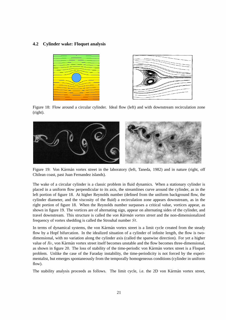
Figure 18: Flow around a circular cylinder. Ideal flow (left) and with downstream recirculation zone(right).
Figure 19: Von Karman vortex street in the laboratory (left, Taneda, 1982) and in nature (right, offChilean coast, past Juan Fernandez islands).
The wake of a circular cylinder is a classic problem in fluid dynamics. When astationary cylinder isplaced in a uniform flow perpendicular to its axis, the streamlines curve around the cylinder, as in theleft portion of figure 18. At higher Reynolds number (defined from the uniform background flow, thecylinder diameter, and the viscosity of the fluid) a recirculation zone appears downstream, as in theright portion of figure 18. When the Reynolds number surpasses a critical value, vortices appear, asshown in figure 19. The vortices are of alternating sign, appear on alternating sides of the cylinder, andtravel downstream. This structure is called thevon Karman vortex streetand the non-dimensionalizedfrequency of vortex shedding is called the Strouhal numberSt.
In terms of dynamical systems, the von Karman vortex street is a limit cycle created from the steadyflow by a Hopf bifurcation. In the idealized situation of a cylinder of infinite length, the flow is two-dimensional, with no variation along the cylinder axis (called the spanwise direction). For yet a highervalue ofRe, von Karman vortex street itself becomes unstable and the flow becomes three-dimensional,as shown in figure 20. The loss of stability of the time-periodic von Karman vortex street is a Floquetproblem. Unlike the case of the Faraday instability, the time-periodicity is not forced by the experi-mentalist, but emerges spontaneously from the temporally homogeneous conditions (cylinder in uniformflow).
The stability analysis proceeds as follows. The limit cycle, i.e. the 2D von Karman vortex street,
21
U2D(x, y, t) the limit cycle is a periodic time-dependent solution to the Navier-Stokes equations:
∂tU2D = −(U2D · ∇)U2D −∇P2D +1
Re∆U2D (68)
The domain is taken to be very large in the(x, y) directions. The velocity is zero on the surface of thecylinder and equal to the imposed uniform flow at infinity.
The perturbationu3D is a solution to the Navier-Stokes equations linearized aboutU2D(t):
∂tu3D = −(U2D(t) · ∇)u3D − (u3D · ∇)U2D(t)−∇p3D +1
Re∆u3D (69)
The perturbed velocity obeys homogeneous boundary conditions on the surface of the cylinder and atinfinity. Equation (69) is homogeneous in the spanwise directionz (along the cylinder). Since werequire that solutions be bounded, the solutions are trigonometric, of formeiβz, and the solution for eachβ evolves independently of the others. Equation (69) is a Floquet problem intime t via the periodic flowU2D(t) about which we linearize. We can therefore decomposeU3D(t) into
u3D ∼ eiβzeλβtfβ(x, y, t) (70)
where the Floquet functionsfβ(x, y, t) are periodic in time and the Floquet multipliers areµβ = eλβT .For eachβ, there is a set of Floquet functions and multipliers. The largest are computed numerically andused to determine the stability of the von Karman vortex streetU2D(t), in particular the wavenumberβand Reynolds number at which the modulus of one of the multipliers|µβ | first exceeds one in modulus.
This Floquet analysis was carried out numerically by Barkley and Henderson in 1995-6. There areactually two bifurcations, to modes with different wavenumbersβ at different Reynolds numbersRe, asshown in figure 20. It turns out that the limit cycle undergoes asteadybifurcation, i.e.µ traverses theunit circle at 1, not at−1 nor ate±iθ, as shown in figure 21. Thus, the temporal behavior of the new 3Dsolutions is similar to that of the 2D flow. The bifurcation is a circle pitchfork, in that any spatial phasein z is permitted.
The 3D transitions of the cylinder wake illustrate several other bifurcation phenomena. First, the bi-furcation to mode A is slightly subcritical, while that to mode B is supercritical. This can actually bedetermined by using a single timeseries near the bifurcation. Figure 22 showsthat both transitions be-gin with exponential growth, at the rate of the computed Floquet multiplier and then deviate from theexponential curve. However, when the transition to mode A first deviates,it is abovethe exponentialcurve, i.e. the nonlinear effects initially increase the instability. In contrast, when the transition to modeB first deviates, it isbelowthe exponential curve, i.e. the nonlinear effects initially decrease. We writethe dynamical system governing the transitions as
An+1 =(
µA + αA|An|2)
An (71)
Bn+1 =(
µB + αB|Bn|2)
Bn (72)
whereAn, Bn represent modesA andB at the same instant in the von Karman vortex shedding period.The complex coefficients describe the amplitude and spanwise phase of a state produced by a circlepitchfork. Figure 22 shows thatαA > 0, whileαB < 0. In order to saturate mode A, a fifth-order termmust be added:
An+1 =(
µA + αA|An|2An + βA|An|4)
An (73)
whereβA < 0.
22

Figure 20: Three-dimensional flow past a cylinder. Left: atRe = 210, mode A with a wave-length near four times the cylinder diameter. Right: atRe = 250, mode B with a wavelengthnear the cylinder diameter. From M.C. Thompson, Monash University, Australia. (http://mec-mail.eng.monash.edu.au/∼mct/mct/docs/cylinder.html)
Figure 21: Floquet multipliers as a function of Reynolds numberRe and spanwise wavenumberβ. Left:Onset of instability to mode A (µ = 1) at Re = 188.5 andβ = 1.585. (wavelength2π/β = 3.96).Right: Onset of instability to mode B (µ = 1) for Re = 259 andβ = 7.64 (wavelength2π/β = 0.822).From Barkley & Henderson, J. Fluid Mech.322, 215 (1996).
23

Figure 22: Transition in time to mode A (left) and mode B (right). Both transitions begin with exponen-tial growth at the rate of the computed Floquet multiplier. Mode A then grows faster than exponentially,indicating a subcritical bifurcation, while mode B grows slower than exponentially, indicating a super-critical bifurcation.
Figures 23 and 24 show that, when increasingRe, mode A is observed, then a mixture of modes A andB, and finally mode B. These figures show experimental measurements and modes A and B are identifiedby their characteristic spatial wavelength and temporal frequency. These facts imply that modes A andB interact. Their symmetries can be taken into account to determine the invariantsand equivariants. Aminimal set of equations reproducing the behavior of the transitions is:
An+1 =(
µA + αA|An|2 + γA|Bn|2 + βA|An|4)
An (74)
Bn+1 =(
µB + αB|Bn|2 + γB|An|2)
Bn (75)
Nonlinear simulations of the 3D Navier-Stokes equations can be used to determine the values ofα, βandγ. Solutions to this minimal model (74)-(75) with these coefficients are shown in figure 25.
24
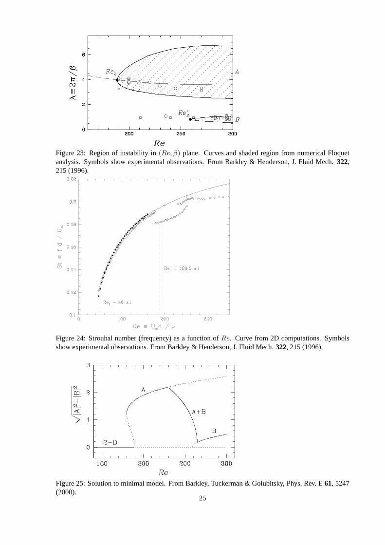
Figure 23: Region of instability in(Re, β) plane. Curves and shaded region from numerical Floquetanalysis. Symbols show experimental observations. From Barkley & Henderson, J. Fluid Mech.322,215 (1996).
Figure 24: Strouhal number (frequency) as a function ofRe. Curve from 2D computations. Symbolsshow experimental observations. From Barkley & Henderson, J. Fluid Mech.322, 215 (1996).
Figure 25: Solution to minimal model. From Barkley, Tuckerman & Golubitsky, Phys. Rev. E61, 5247(2000).
25
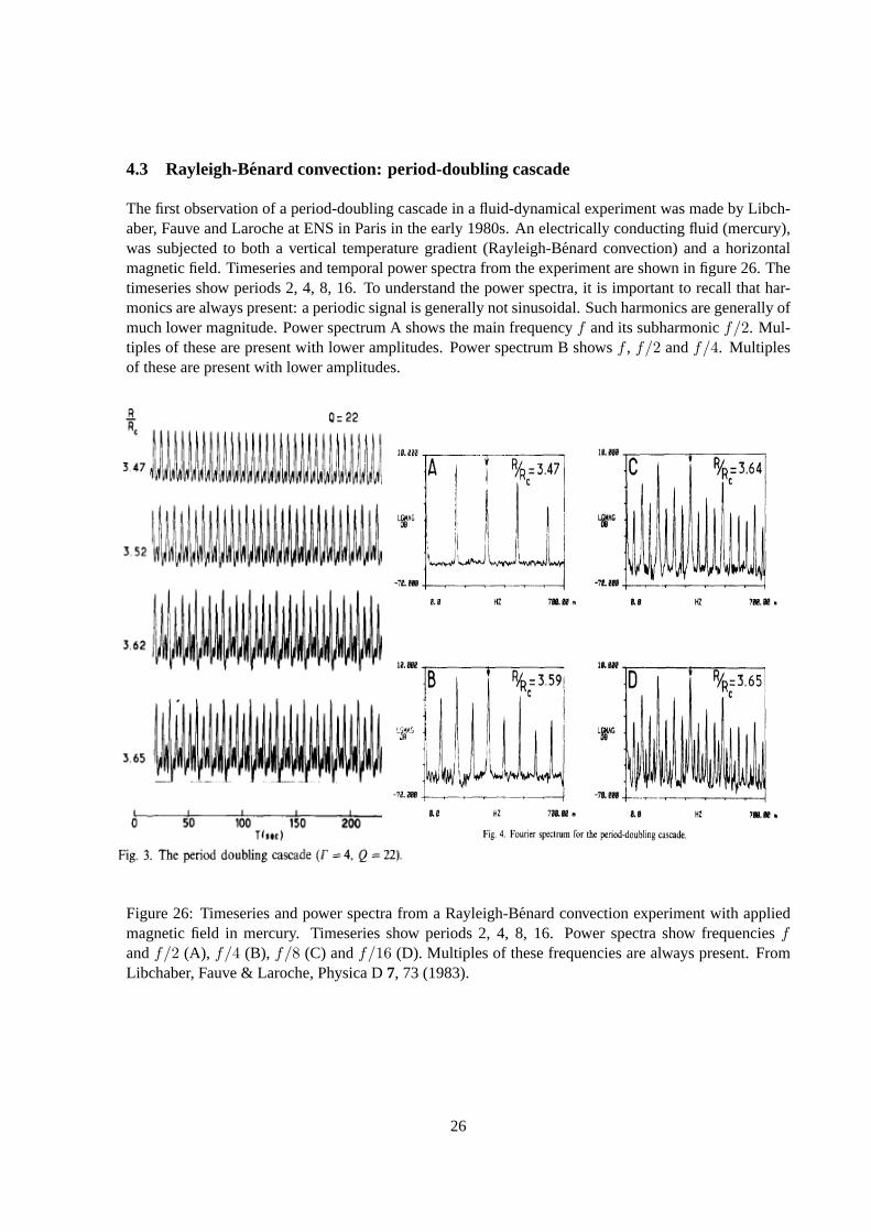
4.3 Rayleigh-Benard convection: period-doubling cascade
The first observation of a period-doubling cascade in a fluid-dynamicalexperiment was made by Libch-aber, Fauve and Laroche at ENS in Paris in the early 1980s. An electrically conducting fluid (mercury),was subjected to both a vertical temperature gradient (Rayleigh-Benard convection) and a horizontalmagnetic field. Timeseries and temporal power spectra from the experiment are shown in figure 26. Thetimeseries show periods 2, 4, 8, 16. To understand the power spectra, itis important to recall that har-monics are always present: a periodic signal is generally not sinusoidal.Such harmonics are generally ofmuch lower magnitude. Power spectrum A shows the main frequencyf and its subharmonicf/2. Mul-tiples of these are present with lower amplitudes. Power spectrum B showsf , f/2 andf/4. Multiplesof these are present with lower amplitudes.
Figure 26: Timeseries and power spectra from a Rayleigh-Benard convection experiment with appliedmagnetic field in mercury. Timeseries show periods 2, 4, 8, 16. Power spectra show frequenciesfandf/2 (A), f/4 (B), f/8 (C) andf/16 (D). Multiples of these frequencies are always present. FromLibchaber, Fauve & Laroche, Physica D7, 73 (1983).
26

4.4 Lorenz system
Although the Lorenz system is not really fluid-dynamical, we will nevertheless discuss it here. Figure27 shows a trajectory of the Lorenz system for the standard chaotic parameter value ofr = 28. Thetrajectory jumps between the two lobes, as also seen on the timeseries ofX(t). One may make afirstreturn mapin the 3D(X,Y, Z) space by drawing a plane and retaining the crossings through the plane,e.g.Z = r − 1. Or one may choose successive maxima, e.g.Z = 0, Z < 0. Either of these proceduresdefines a 2D discrete map. It may happen that the map is in fact 1D, becausethe dissipation is strong.This is seen in figure 28, in which successive maxima ofZ are plotted, i.e.Zk+1 vs. Zk. The factthat these lie on a curve instead of being scattered shows that the dynamics on the Lorenz attractor areeffectively governed by a 1D mapping. This mapping has an unstable fixedpoint and resembles the tentmap shown in figure 10.
Figure 27: Left: 3D trajectory of the Lorenz system for standard chaoticvalue of r = 28. Right:corresponding timeseries. Above: timeseries ofX(t). Below: timeseries ofZ(t). From P. Manneville,Course notes.
Figure 28: First return map for the Lorenz attractor. Successive pairsof maxima ofZ are plottted. FromP. Manneville, Course notes.
27
5 Exercises
1. Consider the discrete-time dynamical system
xn+1 = f(xn) = αxn + x3n
The parameterα may take on positive or negative values.
a. Determine the fixed points and their stability.
b. Determine the location and nature of bifurcations undergone by the fixed points and describe the newstates resulting from the bifurcations.
c. Draw the corresponding bifurcation diagram plottingx as a function ofα, indicating stable andunstable branches and labeling each bifurcation.
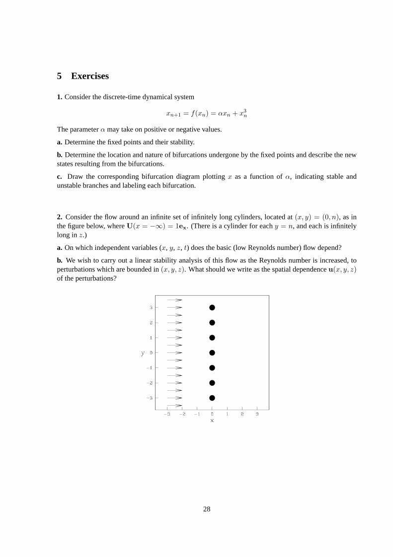
2. Consider the flow around an infinite set of infinitely long cylinders, located at (x, y) = (0, n), as inthe figure below, whereU(x = −∞) = 1ex. (There is a cylinder for eachy = n, and each is infinitelylong inz.)
a. On which independent variables (x, y, z, t) does the basic (low Reynolds number) flow depend?
b. We wish to carry out a linear stability analysis of this flow as the Reynolds number is increased, toperturbations which are bounded in(x, y, z). What should we write as the spatial dependenceu(x, y, z)of the perturbations?
28