Journal of Computer-Aided Molecular Design, 7 (1993) 71 82 71 ESCOM

J-CAMD 182

Nonlinear dependence in comparative molecular field analysis

Ki H w a n K i m

Computer Assisted Molecular Design, Pharmaceutical Products Division, Abbott Laboratories, Abbott Park, IL 60064, [LS.A.

Received 15 January 1992 Accepted 23 June 1992

Key words." 3D QSAR; Comparative molecular field analysis (CoMFA); GRID; Parabolic; Bilinear; Nonlinear; Hydrophobicity

S U M M A R Y

The applicability of the comparative molecular field analysis (CoMFA) approach to describe the nonlin- ear dependence of biological activity on lipophilicity in 3D quantitative structure-activity relationships (QSAR) has been demonstrated. The results indicate that the CoMFA approach is appropriate for describ- ing nonlinear effects in 3D QSAR studies.

I N T R O D U C T I O N

In biological quantitative structure-activity relationships (QSAR), the biological responses elicited by drugs are usually correlated with a combination of hydrophobic, steric, and electronic properties of the molecules. It is well known that the relationships between the biological activity and the physicochemical properties of the compounds are often nonlinear. This is especially true for the hydrophobicity of drugs.

Several models have been proposed to describe such nonlinear relationships. The most often used models are the parabolic model, proposed by Hansch and Clayton [1], and the bilinear model, proposed by Kubinyi [2]. Advantages and disadvantages of these as well as other models have been discussed in the literature [3]. One limitation of these classic models is that they do not include consideration of 3D structures. In the CoMFA method [4], the model is derived from the 3D structure of the molecules by calculating the interaction energies at the 3D lattice points. The resulting correlations are displayed as a 3D coefficient contour map, thus including 3D informa- tion.

In the previous study, CoMFA methodology was used to predict the Hammett (y and pKa's as well as some steric parameters including E s [5-7]. We reported our findings on the parameteriza- tion of hydrophobic effects directly from 3D structures using a CoMFA approach with GRID

0920-654X]$10.00 © 1993 ESCOM Science Publishers B.V.

72

force field [8]. In this study we report an investigation of the applicability of CoMFA methodolo- gy on nonlinear relationships.

Eleven sets of biological data from the literature were selected to demonstrate the applicability of the CoMFA methodology in describing a nonlinear dependence in 3D QSAR. A water probe and the GR ID force field [9] were used in the analysis to describe the hydrophobic effects. In order to compare the CoMFA nonlinear model with the parabolic and bilinear models, biological data that have been reported with the parabolic and bilinear models were selected.

METHODS

Molecular modeling

The starting coordinates were generated using the graphics modeling package for small mole- cules at Abbott or with the program CONCORD [10]. Since no information about the active conformation was available, all the alkyl substituents were chosen to be in an extended conforma- tion. All geometric variables were optimized with AM1 of AMPAC [11]. The molecules in each set were aligned by superimposing the benzyldimethylammonium moiety.

CoMFA interaction energy calculation

The hydrophobic potential energy fields of each molecule were calculated at various lattice points surrounding the molecule using a H20 probe group with the program GRID. A van der Waals radius of 1.70 and a charge of 0.0 were used for the H20 probe with two hydrogen-

bond-donating and two hydrogen-bond-accepting properties. For each substituted alkylbenzyldimenthylammonium chloride molecule, the energies at a total

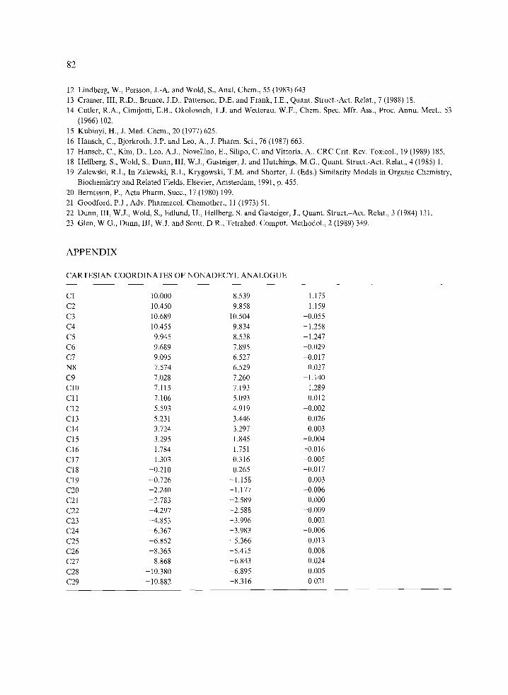
of 3168 grid points were calculated with 2 ,~ spacing in a lattice of 34 x 30 x 20 (X = -17 to 17, Y = -14 to 16, Z = -9 to 11). All energy values greater than 4.0 kcal/mol were truncated to 4.0. Any lattice point for which the standard deviation of the energies was less than 0.05 was discard- ed. These procedures reduced the number of lattice points to 175, 183, 173, 173, 187, 187, 187, 187, 178, 173, and 178 for Eqs. 1A-11A, respectively. The Cartesian coordinates of a nonadecyl

analogue are given in the Appendix as a reference compound.

Partial least-squares (PLS) calculations

Seven or less orthogonal latent variables were first extracted by the standard PLS algorithm [12]. The number of latent variables extracted was always at least 3 less than the number of the compounds included in the correlation. These latent variables were subjected to the PLS cross- validation test [12,13] in the original order of extraction or in the order of their correlation with the dependent variable. The 'best' correlation model was chosen on the basis that it significantly minimized the sum of squares of the difference in activity between the predicted and observed values using predictions made from a leave-one-out jackknife validation test. After the number of latent variables was established, the 'best' correlation model was derived. The final model was further validated by the overall and the stepwise F-statistics. If F-statistics did not support the model, the least significant latent variable was eliminated and the model was rederived. The

73

variables Z1H,o and Z2H2o in the correlation equations are the first and second latent variables from a H20 probe obtained from the PLS analysis of each example.

RESULTS

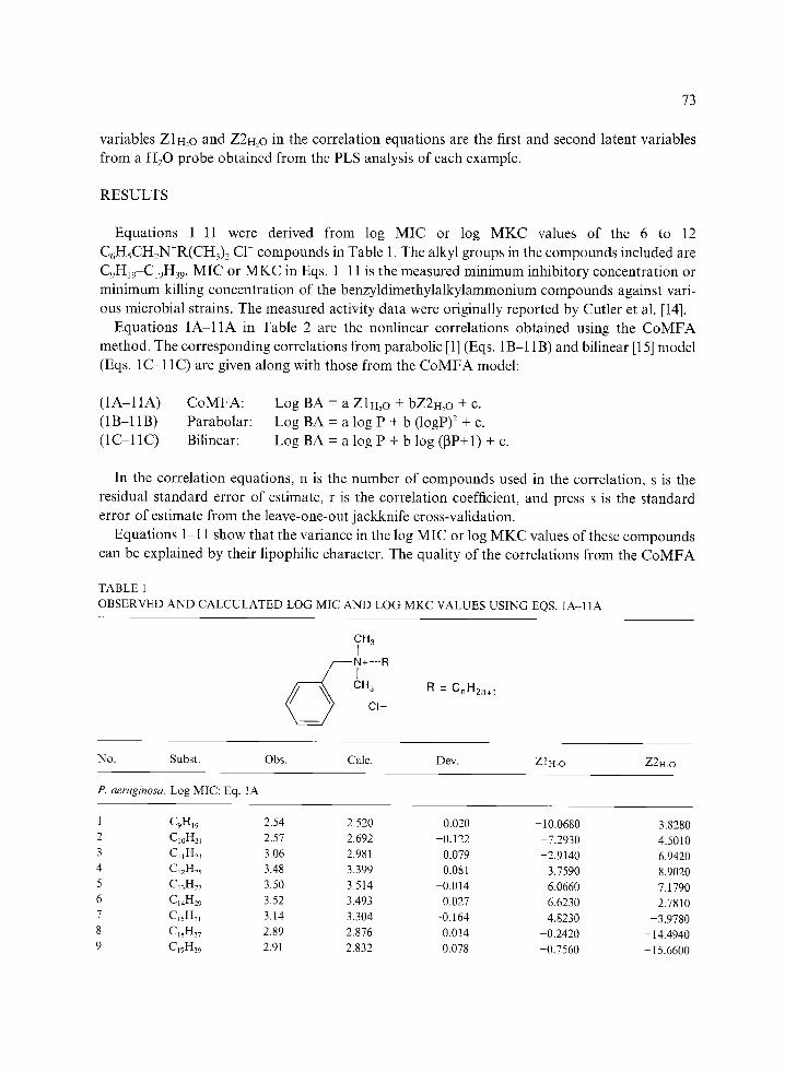
Equations 1-11 were derived from log MIC or log MKC values of the 6 to 12 C6HsCH2N+R(CH3)~ C1 compounds in Table 1. The alkyl groups in the compounds included are C9H19 C19H39. MIC or MKC in Eqs. 1 11 is the measured minimum inhibitory concentration or minimum killing concentration of the benzyldimethylalkylammonium compounds against vari- ous microbial strains. The measured activity data were originally reported by Cutler et al. [14].

Equations 1 A l l A in Table 2 are the nonlinear correlations obtained using the CoMFA method. The corresponding correlations from parabolic [1] (Eqs. 1B 11 B) and bilinear [15] model (Eqs. 1C-11C) are given along with those from the CoMFA model:

(1A-11A) CoMFA: (1B-11B) Parabolar: (1C 11C) Bilinear:

Log BA = a Z1H2o + bZ2H2o + c. Log BA = a log P + b (logP) 2 + c. Log BA = a log P + b log (I3P+I) + c.

In the correlation equations, n is the number of compounds used in the correlation, s is the residual standard error of estimate, r is the correlation coefficient, and press s is the standard error of estimate from the leave-one-out jackknife cross-validation.

Equations 1 11 show that the variance in the log MIC or log MKC values of these compounds can be explained by their lipophilic character. The quality of the correlations from the CoMFA

TABLE 1

OBSERVED AND CALCULATED LOG MIC AND LOG MKC VALUES USING EQS. 1A-1 IA

CH 3 [

CH 3

C I -

R = CnH2n+l

No. Subst. Obs. Calc. Dev. Zlmo Z2H,o

P. aeruginosa. Log MIC: Eq. 1A

1 C9H19 2.54 2.520 0.020 -10.0680 3.8280 2 C10H21 2.57 2.692 -0.122 -7.2930 4.5010 3 Cl1H23 3.06 2.981 0.079 -2.9140 6.9420 4 CI2H25 3.48 3.399 0.08I 3.7590 8.9020 5 C~ 3H27 3.50 3.514 -0.014 6.0660 7.1790 6 C14H29 3.52 3.493 0.027 6.6230 2.7810 7 C~sH~I 3.14 3.304 -0.164 4,8230 -3.9780 8 C18H37 2.89 2.876 0.014 -0.2420 -14.4940 9 C19H39 2.91 2.832 0.078 -0.7560 -15.6600

74

TABLE 1 (continued)

No. Subst. Obs. Calc. Dev. Z1H20 Z2H2O

S. typhosa. Log MIC: Eq. 2A

1 CsHI7 3.52 3.481 0.039 - 13.7880 -3.4000 2 C9H19 3.72 3.625 0.095 - 11.9140 -2.1400 3 CloH21 3.74 3.857 -0.117 -8.5870 -0.4510 4 Cll H23 4.06 4.136 -0.076 -5.1000 2.1940 5 C12Ha5 4.61 4.588 0.022 0.7230 6.2550 6 C13H27 4.80 4.772 0.028 3.9150 6.9140 7 C14H29 4.82 4.845 -0.025 6.9260 5.0250 8 C15H31 4.84 4.789 0.051 9.0860 0.9910 9 C16H33 4.68 4.681 -0.001 9.7220 -2.4700

10 CI9H39 4.21 4.225 -0.015 9.0170 -12.9160

P, vulgaris. Log MIC: Eq. 3A

1 C9H19 2.54 2.530 0.010 -13.5330 -3.5870 2 C10H21 2.74 2.752 -0.012 -10.9810 -1.2970 3 Cl1H23 3.06 3.059 0.001 -7.4400 1.8550 4 C~2H25 3.61 3.564 0.046 -1.2230 6.6050 5 C13H27 3.80 3.763 0.037 2.0720 7.5110 6 C14H29 3.65 3.828 -0.178 4.9490 5.7800 7 CI5H31 3.84 3.796 0.044 7.1390 2.5640 8 C16H33 3.68 3.681 -0.001 7.6570 -0.7050 9 C17H35 3.57 3.425 0.145 6.8280 -5.7200

10 C19H39 2.91 3.001 -0.091 4.5320 -13.0050

P. vulgaris. Log MKC: Eq. 4A

1 C9H19 2.54 2.531 0.009 -7.9500 9.4330 2 C10H21 2.74 2.753 -0.013 -5.6290 8.9850 3 CNH23 3.06 3.061 -0.001 -2.4140 8.5420

4 C12H25 3.61 3.576 0.034 3.0120 7.1430 5 Ci3H2v 3.80 3.779 0.021 5.3160 4.7150 6 C14H29 3.65 3.841 -0.191 -6.3220 0.4800 7 C15H3j 3.84 3.764 0.076 5.8110 -2.7030 8 C16H33 3.68 3.576 0.104 4.1140 -5.4780 9 C18H~v 2.71 2.757 -0.047 -3.5190 - 14.7090

10 C19H39 2.60 2.592 0.008 -5.0620 -16.4090

S. aureus. Log MIC: Eq. 5A

1 C8H17 3.69 3.748 -0.058 -15.9100 -5.5870 2 C9H19 4.02 4.058 -0.038 - 13.5410 -3.0780 3 CzoH21 4.74 4.619 0.121 -9.2190 1.4090 4 CllH23 5.06 5.033 0.027 -5.6810 4.3930 5 C12H25 5.61 5.607 0.003 -0.2800 8.0030 6 C13H27 5.80 5.823 -0.023 2.5860 8.5200 7 C14H29 5.82 5.894 -0.074 5.2870 6.9200

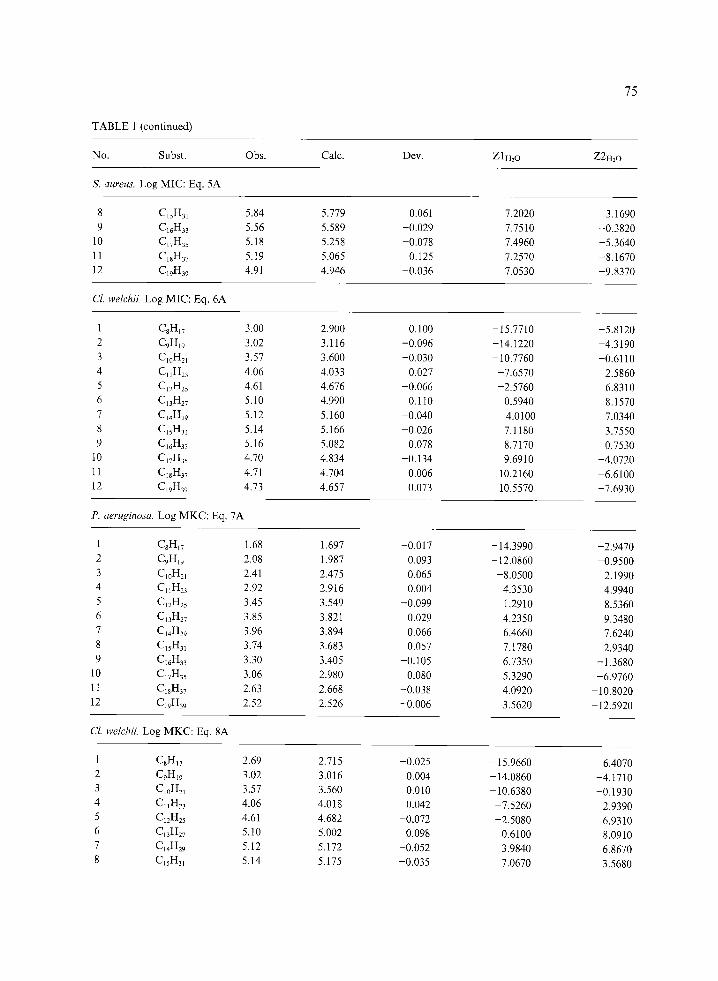
TABLE 1 (continued)

No. Subst. Obs. Calc. Dev. Z 1H20 Z2H_,O

S. aureus. Log MIC: Eq. 5A

75

Cl. welchii Log MIC: Eq. 6A

1 C8HI7 3.00 2.900 0.100 -15.7710 -5.8120 2 C9H19 3.02 3.116 -0.096 -14.1220 -4.3190 3 Cl0H_,l 3.57 3.600 -0.030 - 10.7760 -0.6110 4 Cj1H23 4.06 4.033 0.027 -7.6570 2.5860 5 C12H25 4.61 4.676 -0.066 -2.5760 6.8310 6 Ct3H27 5.10 4.990 0.110 0.5940 8.1570 7 C14H29 5. i2 5.160 -0.040 4.0100 7.0340 8 CjsH~I 5.14 5.166 -0.026 7.1180 3.7550 9 C16H33 5.16 5.082 0.078 8.7170 0.7530

10 C17H35 4.70 4. 834 -0.134 9.6910 -4.0720 11 CI~H37 4.71 4.704 0.006 10.2160 -6.6100 12 C19H39 4.73 4.657 0.073 10.5570 -7.6930

P. aeruginosa. Log MKC: Eq. 7A

1 C8HI7 1.68 1.697 -0.017 -14.3990 -2.9470 2 C9H19 2.08 1.987 0.093 -12.0860 -0.9500 3 C 10H21 2.41 2.475 -0.065 -8.0500 2.1990 4 Ci IH23 2.92 2.916 0.004 -4.3530 4.9940 5 C12H25 3.45 3.549 -0.099 1.2910 8.5360 6 C13H27 3.85 3.821 0.029 4.2350 9.3480 7 C14H29 3.96 3.894 0.066 6.4660 7.6240 8 C15H31 3.74 3.683 0.057 7.1780 2.9340 9 CI6H33 3.30 3.405 -0.105 6.7350 - 1.3680

10 C17H35 3.06 2.980 0.080 5.3290 -6.9760 11 C18H37 2.63 2.668 -0.038 4.0920 -10.8020 12 C19H39 2.52 2.526 -0.006 3.5620 - 12.5920

Cl. welchii. Log MKC: Eq. 8A

1 C8H17 2.69 2.715 -0.025 - 15.9660 -6.4070 2 C9H~9 3.02 3.016 0.004 - 14.0860 -4.1710 3 CIoH21 3.57 3.560 0.010 -10.6380 -0.1930 4 CllH23 4.06 4.018 0.042 -7.5260 2.9390 5 C12H25 4.61 4.682 -0.072 -2.5080 6.9310 6 C13H27 5.10 5.002 0.098 0.6100 8.0910 7 C14H29 5.12 5.172 -0.052 3.9840 6.8670 8 C~sH31 5.14 5. I75 -0.035 7.0670 3.5680

8 CI5H31 5.84 5.779 0.061 7.2020 3.1690 9 C16H33 5.56 5.589 -0.029 7.7510 -0.3820

10 C17H35 5.18 5.258 -0.078 7.4960 -5.3640 11 C18H37 5.19 5.065 0.125 7.2570 -8.1670 12 C19H39 4.91 4.946 -0.036 7.0530 -9.8370

76

TABLE 1 (continued)

No. Subst. Obs. Calc. Dev. Zlrho Z2H2O

Cl. welchii. Log MKC: Eq. 8A

9 C16H33 5.16 5.087 0.073 8.6610 0.6000 10 C17H35 4.70 4.833 -0.133 9.6610 -4.0760 11 CI 8I-I37 4.71 4.700 0.010 10.1990 -6.5430 12 CI9H39 4.73 4.651 0.079 10.5420 -7.6070

Red cell sheep. Log C~50: Eq. 9A

1 CgHI7 1.52 1.615 -0.095 -15.8230 -6.8530 2 C10H21 3.45 3.244 0.206 -8.5620 3.3970 3 C12H,5 4.34 4.391 -0.051 - 1.0670 7.4320 4 C14H29 4.63 4.777 -0.147 4.6890 4.4400 5 C16H33 4.88 4.827 0.053 9.5080 -1.4250 6 ClsH37 4.60 4.565 0.035 11.2560 -6.9910

C. albieans. Log MKC: Eq. 10A

1 C9H19 2.54 2.594 -0.054 -13.9490 -3.5780 2 CloH2I 3.04 2.989 0.051 - 11.3230 -0.9590 3 Cl1H2~ 3.59 3.468 0.122 -7.9770 2.0180 4 C12Hz5 4.09 4.229 -0.139 -2.2290 6.2440 5 C13H27 4.63 4.643 -0.013 1.3400 8.0200 6 C 14H29 4.82 4.915 --0.095 4. 8020 7.8700 7 C15H31 5.14 4.908 0.232 7.0870 5.0780 8 C16H33 4.56 4.649 -0.089 7.2590 1.1260 9 CI7H35 4.16 4.115 0.045 5.9850 -5.1030

10 C18H37 3.59 3.709 -0.119 4.7140 -9.4650 11 C19H39 3.61 3.552 0.058 4.2930 -11.2510

Red cell sheep, Log Cns0: Eq. 11A

1 C8H17 1.76 1.794 -0.034 - 15.2830 -6.6450 2 CloH21 2.95 2.865 0.085 -9.2760 2.0000 3 CI2H~5 3.82 3.869 -0.049 -2.0040 6.9270 4 CI4H~_9 4.40 4.448 -0.048 4.4230 5.4600 5 C16H33 4.79 4.715 0.075 10.0180 -0.2780 6 C18H37 4.52 4.550 -0.030 12.1220 -7.4650

mode l is excellent wi th relatively small s tandard deviat ions and high corre la t ion coefficients. The

press s's o f these correla t ions are excellent consider ing the 'pa rabol ic ' or 'bi l inear ' nature o f the

corre la t ions and the s tandard deviat ions of o ther equat ions f rom the parabol ic or bi l inear model .

The single variable models account for 63 96% of the var iance in the da ta depending on the

nature of the microbia l strains. The addi t ion o f the second latent var iable explains 95-99.7% of

the total var iance in the data. The average s tandard devia t ion and the corre la t ion coefficient of

TABLE 2 S U M M A R Y OF CoMFA, PARABOLIC ", AND BILINEAR b MODELS

77

(1A l l A ) CoMFA: Log BA r = a Z1H~o + b Z2m o + c (1B l lB) Parabolar: L o g B A = a l o g P + b ( l o g p ) 2 + c (1 ~ 1 1 C) Bilinear: Log BA = a log P + b log (~P+ I) + c

Eq. d a b c n s r log Pg

1A 0.059 (+ 0.006) 0.012(+ 0.004) 3.068 (+ 0.034) 9 0.102 0.973 1,82 1B 0.55 (+ 0.30) -0.13 (+ 0.07) 2.85 (+ 0.26) 9 0.208 0.880 2.13 1C 0.766 (+ 0.73) -1.033(+ 0.66) 2.866 (+ 0.31) 9 0.168 0.937 1,56 2A 0.049 (+ 0.003) 0.040(+ 0.004) 4.300 (+ 0.022) 10 0.071 0.993 2.32 2B 0.57 (-+ 0.18) -0.12 (_+ 0.05) 4.08 (-+ 0.17) 10 0.183 0.949 2.38 2C 0.552 (_+ 0.20) -0.937(_+ 0.30) 3.998 (+ 0.15) 10 0.140 0.975 2.19 3A 0.048 (_+ 0.004) 0.043(_+ 0.005) 3.340 (+ 0.031) 10 0.098 0.984 2.32 3B 0.78 (+ 0.16) -0 . I8 (+ 0.04) 2.93 (_+ 0.15) 10 0.123 0.974 2.21 3C 0.675 (+ 0.26) -1.186(_+ 0.31) 2.878 (_+ 0.17) 10 0.132 0.974 2.10 4A 0.097 (+ 0.005) 0.008(_+ 0.003) 3.223 (_+ 0.029) 10 0.090 0.989 2.32 4B 0.84 (_+ 0.23) -0.21 (_+ 0.06) 2.94 (+ 0.20) 10 0.172 0.960 1,97 4C 0.683 (+ 0.29) -1.439(_+ 0.35) 2.879 (_+ 0.19) 10 0.153 0.973 2 !02 5A 0.064 (-+ 0.003) 0.063(-+ 0.004) 5.118 (+ 0.022) 12 0.077 0.995 2.22 5B 0.90 (-+ 0.14) -0.21 (+ 0.04) 4.80 (-+ 0.14) 12 0.158 0.979 2.18 5C 1.047 (_+ 0.19) -1.507(_+ 0.19) 4.757 (+ 0.12) 12 0.100 0.993 1.79 6A 0.071 (+ 0.003) 0.066(_+ 0.005) 4.410 (_+ 0.025) 12 0.088 0.995 2.82 6B 0.91 (_+ 0.21) -0.17 (+ 0.06) 3.87 (_+ 0.21) 12 0.230 0.966 2.68 6C 0.942 (_+ 0.26) -1.274(_+ 0.31) 3.774 (+ 0.18) 12 0.172 0.983 2.25 7A 0.077 (_+ 0.003) 0.057(_+ 0.003) 2.967 (+ 0.022) 12 0.075 0.996 2.32 7B 0.93 (_+ 0.20) -0.23 (+ 0.05) 2.76 (_+ 0.20) 12 0.220 0.962 1.99 7C 0.983 (+ 0.i9) -1.715(+ 0.22) 2.643 (_+ 0.13) 12 0.122 0.990 1.86 8A 0.076 (_+ 0.002) 0.071(_ + 0.004) 4.384 (_+ 0.022) 12 0.075 0.997 2.82 8B 0.99 (+ 0.17) -0.19 (_+ 0.05) 3.80 (_+ 0.17) 12 0.190 0.980 2.65 8C 1.061 (_+ 0.20) -1.376(_+ 0.23) 3.723 (_+ 0.14) 12 0.125 0.992 2.18 9A 0.109 (-+ 0.007) 0.081(_+ 0.012) 3.903 (_+ 0.067) 6 0.163 0.995 2.92 9B 1.26 (_+ 0.35) -0.24 (_+ 0.11) 3.31 (+ 0.37) 6 0.213 0.991 2.59 9C 2.139 (_+ 1.85) -2.118(_+ 1.71) 3.871 (_+ 1.82) 6 0.171 0.996 -r I0A 0.082 (+ 0.005) 0.069(+ 0.006) 3.979 (-+ 0.038) 11 0.128 0.989 2.32 10B 1.34 (+- 0.31) -0.30 (+ 0.08) 3.25 (-+ 0.28) 11 0.243 0.96I 2.25 10C 1.150 (_+ 0.31) -2.041(_+ 0.37) 3.159 (_+ 0.21) 11 0.170 0.984 2.16 l l A 0.102 (_+ 0.003) 0.053(_+ 0.006) 3.707 (_+ 0.033) 6 0.081 0.998 2.92 l l B 1.04 (_+ 0.14) -0.16 (+ 0.04) 3.05 (_+ 0.15) 6 0.084 0.998 3.15 l l C 1.006 (_+ 0.50) -1.191(_+ 0.95) 2.919 (+ 0.40) 6 0.154 0.996 2.72

~Ref. 1. bRef. 2. el: P. aerugh~osa (Log MIC); 2: S. typhosa (Log MIC); 3: P. vulgaris (Log MIC); 4: P. vulgaris (Log MKC); 5: S. aureus (Log MIC); 6: Cl. welchii (Log MIC); 7: P. aeruginosa (Log MKC); 8: Cl. welchii (Log MKC); 9: Red ceil sheep (Log CHs0); 10: C. albicans (Log MKC); Red cell sheep (Log CHs0).

q A : F = 52.3, P = 0.0002, press s -- 0.161; 2A: F = 235.1, P = 0.0001, press s = 0.202; 3A: F = 104.9, P = 0.0001, press s = 0.267; 4A: F = 158.0, P = 0.000l, press s = 0.197; 5A: F = 443.0, P = 0.0001, press s = 0.206; 6A: F = 461.8, P = 0.0001, press s = 0.156; 7A: F = 511.6, P = 0.0001, press s = 0.198; 8A: F = 714.0, P = 0.0001, press s = 0.183; 9A: F = 149.1, P = 0.001, press s = 0.855; 10A: F = 188.1, P = 0.0001, press s = 0.277; I1A: F = 514.3. P = 0.0002, press s = 0.540.

eLog Po values for the C o M F A model were estimated from 3D coefficient contour maps. fLog Po could not be determined.

78

Fig. 1. Stereoscopic view of the major hydrophobic feature of Eq. 19. The positive contour region (in red) increases the antimicrobial potency and the negative contour region (in blue) decreases the potency. The nonadecyl analogue is used as a reference structure. (The contour is shown at 0.003 level.)

the C o M F A models are 0.095 and 0.990, respectively. In contrast, they are 0.184 and 0.964 for the parabolic models and 0.146 and 0.981 for the bilinear models.

Figure 1 is the coefficient contour plot of the correlation described in Eq. 7A*. The contour

maps from other CoMFA models are not presented here, but they are similar to that of Eq. 7A.

The area where hydrophobic substituents contribute positively towards increasing the antimicro-

bial potency is shown by the positive contour (in red), while the area where hydrophobic substit- uents contribute negatively is shown by the negative contour (in blue). Figure 2 is the plot between

the observed and calculated log MIC values using Eq. 7A.

Table 1 lists the observed and calculated log MIC or log MKC values of the compounds

included using Eqs. 1A-11A. Equations 1-11 show that the molecular fields calculated with a H20 probe produced correla-

tions with an excellent standard error of estimate and a correlation coefficient compared to those

*Different contour levels show different degrees of the effects described by the positive and negative contours. The small patches of the contours in Fig. 1 are due to the small differences in the geometries and may be considered as noise.

79

OBSD

4 O:

3 ,5

8 0-

0

5 3 t ~ . . . . . . . I . . . . . . . . . I . . . . . . . . . I . . . . . . . . . I . . . . . . . . . I

_ 5 2 . 0 8 . 5 3 . 0 3 . 5 4 . 0

CALC

Fig. 2. Plot of observed vs. calculated log MKC using Eq. 7A.

with log P from the parabolic or bilinear model. The results demonstrate the applicability of the

C o M F A methodology for describing nonlinear relationships in 3D QSAR.

DISCUSSION

In biological QSAR, nonlinear relationships between the lipophilicity of drugs and their activi-

ties are well known. Among the several models [3] that have been proposed to describe nonlinear

relationships, the parabolic model and the bilinear model are used the most often.

The coefficient contour map of the nonlinear C o M F A models shows a characteristic pattern.

Unlike the linear model where the positive or negative contours may prevail, depending on the

sign of the coefficient, both contours are present and located next to one another in the nonlinear

model. The positive contours correspond to the left side (ascending slope) of the optimum log P,

while the negative contours correspond to the right side (descending slope) of the log Po in the

parabolic or bilinear model. Valuable information obtained from a parabolic or bilinear model is

the optimum lipophilicity of the drug, log Po. The usefulness of log Po has been well demonstrated

in the past [16,17]. In the present examples, where the substituents are n-alkyl groups, this information can be easily obtained from the C o M F A results. The region at the end of the positive

contours appears to correspond to the optimum log Po value in these particular examples. At

present, the log Po values are manually calculated from the coefficient contours*. Nonetheless,

*Because the structural variation is unidirectional, it was relatively simple to calculate the log Po values in these examples. The log Po values were calculated from the corresponding coefficient contours by first estimating the 'optimum' length of the "alkyl' substituent, which corresponds to the end of the positive contour region toward the negative contour region. The log Po value was then calculated by an interpolation for that optimum length of alkyl moiety from a linear plot of log P values for various n-alkyl groups. The calculated log MIC or MKC values were also compared in order to verify the proper selection of the optimum length of the alkyl substituent.

8 0

10

5 -

0 -

- 5

- 10 -

- 15 -

- 20 5

10

5

0

- 5 -

- 10

- 15

-2O 0

15

5

0

- 5

- 10

- 15 - 15

[]

. l l 0

Eq . 1 A

[]

o

[]

m n

i I - 5 0 Z1 -N20

E q . 4 A

o

D Q

o 0

I 5 10

o

D

[]

13

o

o

0

i 5 10

Eq . 3 A 10-

o

[]

=

o

' ~ ' - 15 - 1o - 0

Z l -H20

Eq . 6 A

10

o o

5

o

0 []

o - 5 []

[]

; ; , . l o '5 ' ' - 5 - 20 - 115 110 - O 5

Z1-N20 Z1-H20

E q , 7 A Eq . 9 A

8 =

[]

m

D

O

o

D

[] I

5 10

D [] o

[]

[3

o

I 5

Eq , 2 A 10

D

5

0 o

D o

- 5

- 7 0

- 1 5 15 i - 15 -110 - 0

Zl -H20

Eq . 5 A

l o

o

5 o

o

&

o

- 5 D

" 1020 - 0 . . 115 _110 I 5

Z l -H20

Eq. 8 A

70

o D

5

[]

o - 5

[]

- 10 , i 5 10 -20 - 15 -110 - O

Z1 H20

Eq . I O A

8 []

o 5 o

o 2

D

2 -

o

D i - 5 -

'5 ' ' - 0 5 10 Z1+120

[]

o

o

o

o

D o

I 5 110 15

Eq . l l A

[]

o D

10 15

m

. 110 I I 5 10 15

[]

2

o

- 2

- 5

o

.5. . . . . '5 .1'o .; ; Z I IH20 Z l -H20

15

5 -

0 - O

- 5 -

- 1 0 -

-15

13

D

o

D

-5 .2 ° i i 15 I i I n 5 -110 - 15 - 10 0 5 10 15

Z1H2'O

Fig. 3. Plots of the first (Zlm_o) a n d s e c o n d (Z2H2o) la tent var iab les from CoMFA m o d e l s .

they are excellent compared to the optimum log P values from the parabolic or bilinear model and the real optimum in the observed biological activity.

Another characteristic in the nonlinear dependence of the biological activity is seen in the plots between the first and second latent variables (Z 1 H,O and Z2vI2O). Hellberg et al. [18] and Zalewski

81

[19] have previously utilized plots of the latent variables or principal components in the discussion

of their studies. Figure 3 is a collection of the plots between Zli-t,o and Z2H:o f rom Eqs. 1A-11A. It is interesting that these plots resemble a rotated 'parabolic ' or 'bilinear' plot.

In traditional QSAR, it is preferred that the independent variables are orthogonal to each other

in order for the regression analysis to give interpretable results. The presence of squared terms or cross terms usually leads to colinearities in the variables. The inclusion of highly correlated variables does not provide independent information for the regression analysis and may provide

inconsistent and misleading results. In order to achieve good estimates of the regression coeffi-

cients, the independent variables must be relatively orthogonal to each other. Different authors have discussed this subject and proposed methods that can be used to make a linear variable and its square independent of each other [20,21]. In PLS, all the principal components are orthogonal to each other [19,22,23]. Therefore, there is no need for any special treatment to avoid such colinearity problems. This is one of the advantages in the C o M F A methodology and makes the C o M F A treatment of nonlinear cases even more attractive.

The effects of different lattice positions with respect to the molecules were investigated by translating the grid box in X, Y, and Z directions each by 0.5, 1.0, and 1.5 A. Although not identical, the different lattice points gave results that are very similar. A larger number of exclud- ed compounds (up to about 40%) in the jackknife cross-validation tests did not affect the cross-

validation results. Finally, the approaches described here for lipophilic dependence can be applied to the non-

linear dependence of other physicochemical properties, such as steric or electronic properties.

C O N C L U S I O N

Several results are presented showing that the hydrophobic potential energy fields calculated with a H20 probe with the G R I D force field using a C o M F A approach produced significant correlations with excellent cross-validation. The results demonstrate the applicability of the C o M F A approach in describing nonlinear relationships in 3D QSAR studies.

R E F E R E N C E S

1 Hansch, C. and Clayton, J.M., J. Pharm. Sci., 62 (1973) 1. 2 Kubiriyi, H., Arzneim.-Forsch. (Drug Res.), 26 (1976) 1991. 3 Kubinyi, H., QSAR in the Design of Bioactive Compounds. In Proceedings of the First International Telesymposium

in Medicinal Chemistry, 18 February, 1984, J.R. Prous Publ., Barcelona, Spain, pp. 321 346. 4 Cramer, III, R.D., Patterson, D.E. and Bunce, J.D., J. Am. Chem. Soc., 110 (1988) 5959. 5 Kim, K.H. and Martin, Y.C., In Silipo, C. and Vittoria, A. (Eds.) QSAR: Rational Approaches on the Design of

Bioactive Compounds (Proceedings of the 8th European Symposium, Sorrento (Napoli), Italy, 9 13 September, 1990), Elsevier, Amsterdam, 1991, pp. 151-154.

6 Kim, K.H. and Martin, Y.C., J. Org. Chem., 56 (1991) 2723. 7 Kim, K.H. and Martin, Y.C., J. Med. Chem., 34 (1991) 2056. 8 Kim, K.H., Med. Chem. Res., 1 (1991) 259. 9 GRID program, V7, Molecular Discovery Ltd., West Way House, Elms Parade, Oxford, U.K.

10 Rusinko, III, A., Skell, J.M., Balducci, R., McGarity, C.M. and Pearlman, R.S., The University of Texas at Austin and Tripos Associates, St. Louis, MO, I988.

1I Liotard, D.A., Healy, E.F., Ruiz, J.M. and Dewar, M.J.S., AMPAC V 2.1 (QCPE No. 506). Ran with the keywords NOINTER and XYZ.

82

12 Lindberg, W., Persson, J.-A. and Wold, S., Anal. Chem., 55 (1983) 643. 13 Cramer, III, R.D., Brunce, J.D., Patterson, D.E. and Frank, I.E., Quant. Struct.-Act. Relat., 7 (1988) 18. 14 Cutler, R.A., Cimijotti, E.B., Okolowich, T.J. and Wetterau, W.F., Chem. Spec. Mfr. Ass., Proc. Annu. Meet., 53

(1966) 102. 15 Kubinyi, H., J. Med. Chem., 20 (1977) 625. 16 Hansch, C., Bjorkroth, J.P. and Leo, A., J. Pharm. Sci., 76 (1987) 663. 17 Hansch, C., Kim, D., Leo, A.J., Novellino, E., Silipo, C. and Vittoria, A., CRC Crit. Rev. Toxicol., 19 (1989) 185. 18 Hellberg, S., Wold, S., Dunn, III, W.J., Gasteiger, J. and Hutchings, M.G., Quant. Struct.-Act. Relat., 4 (1985) i, 19 Zalewski, R.I., In Zalewski, R.I., Krygowski, T.M. and Shorter, J. (Eds.) Similarity Models in Organic Chemistry,

Biochemistry and Related Fields, Elsevier, Amsterdam, 1991, p. 455. 20 Berntsson, P., Acta Pharm. Suec., 17 (1980) 199. 21 Goodford, P.J., Adv. Pharmacol. Chemother., 11 (1973) 51. 22 Dunn, III, W.J., Wold, S., Edlund, U., Hellberg, S. and Gasteiger, J., Quant. Struct. Act. Relat., 3 (1984) 131. 23 Glen, W.G., Dunn, III, W.J. and Scott, D.R., Tetrahed. Comput. Methodol., 2 (1989) 349.

A P P E N D I X

CARTESIAN COORDINATES OF NONADECYL ANALOGUE

C1 I0.000 8.539 1.175 C2 10.450 9.858 1.159 C3 10.689 10.504 -0.055 C4 10.455 9.834 -1.258 C5 9.945 8.538 -1.247 C6 9.689 7.895 -0.029 C7 9.095 6.527 -0.017 N8 7.574 6.529 0.037 C9 7.028 7.260 - 1.140 C10 7.115 7.193 1.289 Cl l 7.106 5.093 0.012 C12 5.593 4.919 -0.002 C13 5.231 3.446 0.026 C14 3.724 3.297 -0.003 C15 3.295 1.845 -0.004 C16 1.784 1.751 -0.016 C17 1.303 0.316 -0.005 C18 -0.210 0.265 -0.017 C19 -0.726 -1.158 0.003 C20 -2.240 - 1.177 -0.006 C21 -2.783 -2.589 0.000 C22 -4.297 -2.588 -0.009 C23 -4.853 -3.996 0.002 C24 -6.367 -3.983 -0.006 C25 -6.852 -5.366 0.013 C26 -8.365 -5.415 0.008 C27 -8.868 -6.843 0.024 C28 -10.380 -6.895 0.005 C29 -10.882 -8.316 0.021