Chapter 7

Nonholonomic Behavior

in Robotic Systems

In this chapter, we study the e!ect of nonholonomic constraints on thebehavior of robotic systems. These constraints arise in systems suchas multifingered robot hands and wheeled mobile robots, where rollingcontact is involved, as well as in systems where angular momentum isconserved. We discuss the problem of determining when constraints onthe velocities of the configuration variables of a robotic system are inte-grable, and illustrate the problem in a variety of di!erent situations. Theemphasis of this chapter is on the basic tools needed to analyze nonholo-nomic systems and the application of those tools to problems in roboticmanipulation. These tools are drawn both from some basic theorems indi!erential geometry and from nonlinear control theory.

1 Introduction

In the preceding chapter, we derived the equations of motion for a roboticsystem with kinematic constraints. We restricted ourselves to Pfa"anconstraints which had the general form

J(!, x)! = GT (!, x)x, (7.1)

where q = (!, x) ! Rn is the configuration of the system. As we saw,equations of this form could be used to model a large number of roboticsystems, including multifingered hands, robots in contact with their en-vironment, and redundant manipulators.

By shifting our notation slightly, we can write the preceding con-straints in the form

"i(q)q = 0 i = 1, . . . , k, (7.2)

317

where the "i(q) are row vectors. We assume that the "i are linearlyindependent at each point q ! Rn, since if they are not, the dependentconstraints may be eliminated. Each "i describes one constraint on thedirections in which q is permitted to take values.

Recall from Chapter 6 that a constraint is said to be holonomic if itrestricts the motion of a system to a smooth hypersurface of the configu-ration space. It will be convenient to adopt some language and notationfrom di!erential geometry, so we call this smooth hypersurface a manifold.Locally, a holonomic constraint can be represented as a set of algebraicconstraints on the configuration space,

hi(q) = 0, i = 1, . . . , k. (7.3)

The dimension of the manifold on which the motion of the system evolvesis n " k.

We say that a set of k Pfa"an constraints of the form in equation (7.2)is integrable if there exist functions hi : Rn # R, i = 1, . . . , k such that

hi(q(t)) = 0 $% "i(q)q = 0 i = 1, . . . , k.

Thus, a set of Pfa"an constraints is integrable if it is equivalent to a setof holonomic constraints. We often call an integrable Pfa"an constrainta holonomic constraint, although strictly speaking the former is describedby a set of velocity constraints and the latter by a set of functions. A setof Pfa"an constraints is said to be nonholonomic if it is not equivalentto a set of holonomic constraints.

As we saw in Chapter 6, the presence of nonholonomic constraintsrequires special care in deriving the equations of motion for the system.The point of view taken in this chapter is somewhat di!erent. Here, wewill try to understand when we can exploit the nonholonomy of the con-straints to achieve motion between configurations. In particular, we willbe interested in answering the following question: given two points q0

and qf , when does there exist a path q(t) which satisfies the constraintsin equation (7.2) at all times and connects q0 to qf? The set of all pointswhich can be connected to q0 via a path which satisfies the constraints iscalled the reachable set associated with q0. Thus, we wish to understandunder what conditions the reachable set will be the entire configurationspace. This is intimately related to the nonholonomy of the constraints,since if the constraints are holonomic, then the motion of the system isrestricted to the level sets given by hi(q) = hi(q0), i = 1, . . . , k. Hence,for holonomic constraints the reachable set is some subset of the config-uration space which lies in the level set hi(q) = hi(q0), and we cannotmove freely between configurations on di!erent level sets.

A good example of the type of behavior which we wish to exploit isthat of an automobile. The kinematics of an automobile are constrainedbecause the front and rear wheels are only allowed to roll and spin, but

318

not to slide sideways. As a consequence, the car itself is not capableof sliding sideways, or rotating in place. Despite this, we know fromour own experience that we can park an automobile at any position andorientation. Thus, the constraints are not holonomic since the motionof the system is unrestricted. Finding an actual path between two givenconfigurations is an example of a nonholonomic motion planning problemand is the subject of the next chapter.

Checking to see if a constraint is holonomic or nonholonomic is neithereasy nor obvious. Consider first the case in which there is a single velocityconstraint,

"(q)q =n!

j=1

"j(q)qj = 0.

This constraint is integrable if there exists a function h : Rn # R suchthat

"(q)q = 0 $% h(q) = 0.

It follows by di!erentiating h(q) = 0 with respect to time that if thePfa"an constraint is holonomic then

n!

j=1

"j(q)qj = 0 =%n!

j=1

#h

#qjqj = 0.

In turn, this implies that there exists some function $(q), called an inte-grating factor, such that

$(q)"j(q) =#h

#qj(q) j = 1, . . . , n. (7.4)

Thus, a single Pfa"an constraint is holonomic if and only if there existsan integrating factor $(q) such that $(q)"(q) is the derivative of somefunction h.

Equation (7.4) is not very constructive from the point of view of check-ing integrability since it involves the unknown function h(q). This situa-tion may be remedied by using the fact that

#2h

#qi#qj=

#2h

#qj#qi

to get#($"j)

#qi=

#($"i)

#qji, j = 1, . . . , n. (7.5)

Equation (7.5) states that the constraint is equivalent to h(q) = 0 if thereexists some integrating factor $(q) for which the equation (7.5) is true.This should really not be a surprise since

"(q)q = 0 =% $(q)"(q)q = 0

319

for all choices of smooth functions $(q). However, one still has to find afunction $ which satisfies equation (7.5).

The question of integrability becomes much more di"cult in the pres-ence of multiple Pfa"an constraints. Given a set of k constraints of theform of equation (7.2), not only does one need to check whether eachone of the k constraints is integrable, but also which independent linearcombinations of these,

k!

i=1

$i(q)"i(q)q,

are integrable. That is, even if the given constraints are not individuallyintegrable, they may contain a set of integrable constraints. Thus, theremay exist functions hi for i = 1, . . . , p with p & k such that

span{#h1

#q(q), . . . ,

#hp

#q(q)} ' span{"1(q), . . . ,"k(q)}

for all q. If it is possible to find these functions, the motion of the systemis restricted to level surfaces of h, namely to sets of the form

{q : h1(q) = c1, . . . , hp(q) = cp}.

If p = k, then the constraints are holonomic. In the case that p < k, theconstraints are not holonomic (since they are not completely equivalentto a set of holonomic constraints) but the reachable points of the systemare still restricted. Thus the constraints are “partially holonomic.” Wewill be primarily interested in the case in which the constraints do notrestrict the reachable configurations. We refer to this situation as beingcompletely nonholonomic.

It will be convenient for us to convert problems with nonholonomicconstraints into another form. Roughly speaking, we would like to ex-amine the systems not from the point of view of the constraints (namely,the directions that we cannot move), but rather from the viewpoint ofthe directions in which we are free to move. We begin by choosing abasis for the right null space of the constraints, denoted by gj(q) ! Rn,i = 1, . . . , n " k =: m. By construction, this basis satisfies

"i(q)gj(q) = 0i = 1, . . . , k

j = 1, . . . , n " k,

and the allowable trajectories of the system can thus be written as thepossible solutions of the control system

q = g1(q)u1 + · · · + gm(q)um. (7.6)

That is, q(t) is a feasible trajectory for the system if and only if q(t)satisfies equation (7.6) for some choice of controls u(t) ! Rm.

320

In this context, a constraint is completely nonholonomic if the corre-sponding control system can be steered between any two points. Thusthe reachable configurations of the system are not restricted. Conversely,if a constraint is holonomic, then all motions of the system must lie onan appropriate constraint surface and the corresponding control systemcan only be steered between points on the given manifold. Hence, we canstudy the nature of Pfa"an constraints by studying the controllabilityproperties of equation (7.6).

Nonholonomic constraints arise in a variety of applications. Besidesrolling constraints on multifingered hands, nonholonomic constraints playan important role in the study of mobile robot systems and space-basedrobotic systems (in which conservation of angular momentum plays therole of a nonholonomic constraint). For these applications the primaryquestion is that of reachability: when can we find a path between twoarbitrary configurations and how do we go about computing such a path?

The outline of this chapter is as follows: in Section 2 we develop sometools from di!erential geometry and nonlinear control. Section 3 givesexamples of systems with velocity constraints. In Section 4 the structureof nonholonomic systems is explored and the examples of Section 3 areanalyzed. In the next chapter, we will develop methods for planningpaths compatible with nonholonomic constraints.

Both this chapter and Chapter 8 are slightly more advanced in flavorthan the previous chapters and represent some of the recent research inthe robotics literature. Nonholonomic behavior also plays a strong role inmany problems in geometric mechanics, which we touch on only brieflyin the examples and exercises. In classical mechanics, nonholonomic be-havior is closely related to the geometric phase associated with a groupsymmetry in a Hamiltonian or Lagrangian system. A good introductionto these concepts can be found in the lecture notes by Marsden [67].

2 Controllability and Frobenius’ Theorem

In the previous section, we saw the di"culties in trying to determinewhether or not constraints on a system were holonomic (or integrable).Further, if they are not holonomic, it is not completely clear as to whenthey are completely nonholonomic. In this section, we will develop themachinery needed for analyzing nonholonomic systems, in particular foranswering the question of when a set of Pfa"an constraints is holonomic.

The tools we develop are based on a variety of results from di!erentialgeometry and nonlinear control theory, more specifically Frobenius’ theo-rem and nonlinear controllability. To keep the mathematical prerequisitesto a minimum, we do all the calculations in Rn and restrict ourselves todrift-free control systems (i.e., control systems whose state remains fixedwhen the input is turned o!). Many of the proofs in this section rely on

321

some properties of manifolds which we have omitted from the discussion;they can be skipped without loss of continuity. A good introduction tononlinear control theory which includes many of the necessary di!erentialgeometric concepts can be found in Isidori [43] or Nijmeijer and van derSchaft [83].

2.1 Vector fields and flows

We restrict our attention to Rn. We choose to make a distinction, how-ever, between the space and its tangent space at a given point. A pointof contact with Chapter 2 is our insistence there on making a distinctionbetween points and vectors in R3 and enforcing the distinction by aug-menting points by 1 and vectors by 0. Denote by TqRn the tangent spaceto Rn at a point q ! Rn. A vector field on Rn is a smooth map whichassigns to each point q ! Rn a tangent vector f(q) ! TqRn. In localcoordinates, we represent f as a column vector whose elements dependon q,

f(q) =

"

#$

f1(q)...

fn(q)

%

&' .

A vector field is smooth if each fi(q) is smooth.Vector fields are to be thought of as right-hand sides of di!erential

equations:q = f(q). (7.7)

The rate of change of a smooth function V : Rn # R along the flow of fis given by

V =#V

#qf(q) =

n!

i=1

#V

#qifi.

The time derivative of V along the flow of f is referred to as the Liederivative of V along f and is denoted LfV :

LfV :=#V

#qf(q).

Associated with a vector field, we define the flow of a vector fieldto represent the solution of the di!erential equation (7.7). Specifically,%f

t (q) represents the state of the di!erential equation at time t startingfrom q at time 0. Thus %f

t : Rn # Rn satisfies

d

dt%f

t (q) = f(%ft (q)) q ! Rn.

A vector field is said to be complete if its flow is defined for all t. By theexistence and uniqueness theorem of ordinary di!erential equations, for

322

g2

net motion

"&g1

&g2

&g1

"&g2

g1

nonzero

Figure 7.1: A Lie bracket motion.

each fixed t, %ft is a local di!eomorphism of Rn onto itself. Further, it

satisfies the following group property:

%ft ( %f

s = %ft+s,

for all t and s, where ( stands for the composition of the two flows, namely%f

t (%fs (q)).

2.2 Lie brackets and Frobenius’ theorem

Given two vector fields g1 and g2, the map %g1t ( %g2

s stands for the com-position of the flow of g2 for s seconds with the flow of g1 for t seconds.In general, this quantity is di!erent from the map %g2

s (%g1t , which stands

for the composition in reverse order. Indeed, consider the flow depictedin Figure 7.1 starting from q0. It consists of a flow along g1 for & secondsfollowed by a flow along g2 for & seconds, "g1 for & seconds, and "g2 for &seconds. For & small, we may evaluate the Taylor series in & for the stateof the di!erential equation as

q(&) = %g1! (q(0))

= q(0) + &q(0) +1

2&2q(0) + O(&3)

= q0 + &g1(q0) +1

2&2#g1

#qg1(q0) + O(&3),

where the notation O(&k) represents terms of order &k and the partialderivative of g1 is evaluated at q0.

323

Now evaluating at time 2&,

q(2&) = %g2! ( %g1

! (q0)

= %g2! (q0 + &g1(q0) +

&2

2

#g1

#qg1(q0) + O(&3))

= q0 + &g1(q0) +1

2&2#g1

#qg1(q0)

+ &g2(q0 + &g1(q0)) +&2

2

#g2

#qg2(q0) + O(&3)

= q0 + &(g1(q0) + g2(q0))

+1

2&2(

#g1

#qg1(q0) +

#g2

#qg2(q0) + 2

#g2

#qg1(q0)) + O(&3).

Here, we have used the Taylor series expansion for g2(q0 + &g1(q)) =g2(q0) + &"g2

"q g1(q0) + O(&2). At the next step (we invite the reader to

verify this), we get

q(3&) = %!g1! ( %g2

! ( %g1! (q0)

= q0 + &g2(q0)

+&2

2(#g2

#qg2(q0) + 2

#g2

#qg1(q0) " 2

#g1

#qg2(q0)) + O(&3).

Finally, we get

q(4&) = %!g2! ( %!g1

! ( %g2! ( %g1

! (q0)

= q0 + &2(#g2

#qg1(q0) "

#g1

#qg2(q0)) + O(&3).

(7.8)

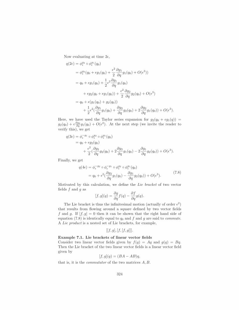
Motivated by this calculation, we define the Lie bracket of two vectorfields f and g as

[f, g](q) =#g

#qf(q) " #f

#qg(q).

The Lie bracket is thus the infinitesimal motion (actually of order &2)that results from flowing around a square defined by two vector fieldsf and g. If [f, g] = 0 then it can be shown that the right hand side ofequation (7.8) is identically equal to q0 and f and g are said to commute.A Lie product is a nested set of Lie brackets, for example,

[[f, g], [f, [f, g]]].

Example 7.1. Lie brackets of linear vector fieldsConsider two linear vector fields given by f(q) = Aq and g(q) = Bq.Then the Lie bracket of the two linear vector fields is a linear vector fieldgiven by

[f, g](q) = (BA " AB)q,

that is, it is the commutator of the two matrices A,B.

324

The following properties of Lie brackets follow from the definition.Their proof is left as an exercise.

Proposition 7.1. Properties of Lie bracketsGiven vector fields f, g, h on Rn and smooth functions $,' : Rn # R,the Lie bracket satisfies the following properties:

1. Skew-symmetry:[f, g] = "[g, f ]

2. Jacobi identity:

[f, [g, h]] + [h, [f, g]] + [g, [h, f ]] = 0

3. Chain rule:

[$f,'g] = $'[f, g] + $(Lf')g " '(Lg$)f,

where Lf' and Lg$ stand for the Lie derivatives of ' and $ alongthe vector fields f and g respectively.

An alternative method of defining the Lie bracket of two vector fieldsf and g is to require that it satisfies for all smooth functions $ : Rn # R:

L[f,g]$ = Lf (Lg$) " Lg(Lf$).

The reader should carefully parse the previous equation and convinceherself of this fact.

A distribution assigns a subspace of the tangent space to each pointin Rn in a smooth way. A special case is a distribution defined by a setof smooth vector fields, g1, . . . , gm. In this case we define the distributionas

# = span{g1, . . . , gm},where we take the span over the set of smooth real-valued functions onRn. Evaluated at any point q ! Rn, the distribution defines a linearsubspace of the tangent space

#q = span{g1(q), . . . , gm(q)} ' TqRn.

The distribution is said to be regular if the dimension of the subspace #q

does not vary with q. A distribution is involutive if it is closed under theLie bracket, i.e.,

# involutive $% )f, g ! #, [f, g] ! #.

For a finite dimensional distribution it su"ces to check that the Lie brack-ets of the basis elements are contained in the distribution. The involutiveclosure of a distribution, denoted #, is the closure of # under bracketing;that is, # is the smallest distribution containing # such that if f, g ! #then [f, g] ! #.

325

Definition 7.1. Lie algebraA vector space V (over R) is a Lie algebra if there exists a bilinear op-eration V * V # V , denoted [ , ], satisfying (i) skew-symmetry and (ii)the Jacobi identity.

The set of smooth vector fields on Rn with the Lie bracket is a Liealgebra, and is denoted X(Rn). Let g1, . . . , gm be a set of smooth vec-tor fields, # the distribution defined by g1, . . . , gm and, # the involutiveclosure of #. Then, # is a Lie algebra (in fact the smallest Lie algebracontaining g1, . . . , gm). It is called the Lie algebra generated by g1, . . . , gm

and is often denoted L(}", . . . , }#). Elements of L(}", . . . , }#) are ob-tained by taking all linear combinations of elements of g1, . . . , gm, takingLie brackets of these, taking all linear combinations of these, and so on.We define the rank of L(}", . . . , }#) at a point q ! Rn to be the dimension

of #q as a distribution.A distribution # of constant dimension k is said to be integrable if for

every point q ! Rn, there exists a set of smooth functions hi : Rn # R,i = 1, . . . , n " k such that the row vectors "hi

"q are linearly independentat q, and for every f ! #

Lfhi =#hi

#qf(q) = 0 i = 1, . . . , n " k. (7.9)

The hypersurfaces defined by the level sets

{q : h1(q) = c1, . . . , hn!k(q) = cn!k}

are called integral manifolds for the distribution. If we regard an integralmanifold as a smooth surface in Rn, then equation (7.9) requires thatthe distribution be equal to the tangent space of that surface at the pointq.

Integral manifolds are related to involutive distributions by the fol-lowing celebrated theorem.

Theorem 7.2 (Frobenius). A regular distribution is integrable if andonly if it is involutive.

Thus, if # is an k-dimensional involutive distribution, then locallythere exist n " k functions hi : Rn # R such that integral manifolds of# are given by the level surfaces of h = (h1, . . . , hn!k). These levelsurfaces form a foliation of Rn. A single level surface is called a leaf ofthe foliation.

Associated with the tangent space TqRn is the dual space T $q Rn, the

set of linear functions on TqRn. Just as we defined vector fields on Rn, wedefine a one-form as a map which assigns to each point q ! Rn a covector"(q) ! T $

q Rn. In local coordinates we represent a smooth one-form as arow vector

"(q) =("1(q) "2(q) · · · "n(q)

).

326

Di!erentials of smooth functions are good examples of one-forms. Forexample, if ' : Rn # R, then the one-form d' is given by

d' =*"#"q1

"#"q2

· · · "#"qn

+.

Note, however, that all one-forms are not necessarily the di!erentials ofsmooth functions (a one-form which does happen to be the derivative ofa function is said to be exact).

A one-form acts on a vector field to give a real-valued function on Rn

by taking the inner product between the row vector " and the columnvector f :

" · f =!

i

"ifi.

A codistribution assigns a subspace of T $q Rn smoothly to each q ! Rn. A

special case is a codistribution obtained as a span of a set of one-forms,

$ = span{"1, . . . ,"m},

where the span is over the set of smooth functions. As before, the rankof the codistribution is the dimension of $q. The codistribution $ is saidto be regular if its rank is constant.

To begin our study of motion planning for nonholonomic systems,our first task is to convert the specified constraints given as one-formsinto an equivalent control system. To this end, consider the problem ofconstructing a path q(t) ! Rn between a given q0 and qf subject to theconstraints

"i(q)q = 0 i = 1, . . . , k.

The "i’s are linear functions on the tangent spaces of Rn, i.e., one-forms.We assume that the "i’s are smooth and linearly independent over theset of smooth functions. The following proposition is a formalization ofthe discussion of the introduction.

Proposition 7.3. Distribution annihilating constraintsGiven a set of one-forms "i(q), i = 1, . . . , k, there exist smooth, linearlyindependent vector fields gj(q), j = 1, . . . , n"k such that "i(q) ·gj(q) = 0for all i and j.

Proof. The "i’s form a codistribution of dimension k in Rn. We canchoose local coordinates such that the set of one-forms is given by

"i =(0 · · · 1 · · · 0 $i,k+1 · · · $in

),

where the 1 in the preceding equation is in the ith entry, and the functions

327

$il : Rn # R are smooth functions. Define

gj :=

"

############$

"$1,(j+k)...

"$k,(j+k)

0...1...0

%

&&&&&&&&&&&&'

,

where the 1 is in the j +kth entry. The gj ’s are linearly independent andannihilate the constraints since

"i · gj = $i(j+k) " $i(j+k) = 0.

This shows that "i · gj = 0 for i = 1, . . . , k and j = 1, . . . , n " k.

In the language of distributions and codistributions, the results of thisproposition are expressed by defining the codistribution

$ = span{"1, . . . ,"k}

and the distribution

# = span{g1, . . . , gn!k}

and stating that# = $%.

We say that the distribution # annihilates the codistribution $. Thecontrol system associated with the distribution # is of the form

q = g1(q)u1 + · · · + gn!k(q)un!k,

with the controls ui to be freely specified.These results of this section can be used to determine if a set of

Pfa"an constraints is holonomic:

Proposition 7.4. Integrability of Pfa!an constraintsA set of smooth Pfa!an constraints is integrable if and only if the distri-bution which annihilates the constraints is involutive.

2.3 Nonlinear controllability

In view of Proposition 7.3, which yields a set of vector fields orthogonalto a given set of one-forms, it is clear that the motion planning problem

328

is equivalent to steering a control system. Thus, we will now restrict ourattention to control systems of the form

% : q = g1(q)u1 + · · · + gm(q)umq ! Rn

u ! U ' Rm.(7.10)

This system is said to be drift-free, meaning to say that when the controlsare set to zero the state of the system does not drift. We assume thatthe gj are smooth, linearly independent vector fields on Rn and thattheir flows are defined for all time (i.e., the gj are complete). We wishto determine conditions under which we can steer from q0 ! Rn to anarbitrary qf ! Rn by appropriate choice of u(·).

A system % is controllable if for any q0, qf ! Rn there exists a T > 0and u : [0, T ] # U such that % satisfies q(0) = q0 and q(T ) = qf . Asystem is said to be small-time locally controllable at q0 if we can reachnearby points in arbitrarily small amounts of time and stay near to q0 atall times. Given an open set V + Rn, define RV (q0, T ) to be the set ofstates q such that there exists u : [0, T ] # U that steers % from q(0) = q0

to q(T ) = qf and satisfies q(t) ! V for 0 & t & T . We also define

RV (q0,&T ) =,

0<$&T

RV (q0, ()

to be the set of states reachable up to time T . A system is small-time lo-cally controllable (locally controllable for brevity) if RV (q0,&T ) containsa neighborhood of q0 for all neighborhoods V of q0 and T > 0.

Let # = L(}", . . . , }#) be the Lie algebra generated by g1, . . . , gm. Itis referred to as the the controllability Lie algebra. From the constructioninvolved in the definition of the Lie bracket in the previous subsection,we saw that by using an input sequence of

u1 = +1 u2 = 0 for 0 & t < &u1 = 0 u2 = +1 for & & t < 2&u1 = "1 u2 = 0 for 2& & t < 3&u1 = 0 u2 = "1 for 3& & t < 4&,

we get motion in the direction of the Lie bracket [g1, g2]. If we were toiterate on this sequence, it should be possible to generate motion alongdirections given by all the other Lie products associated with the gi.Thus, it is not surprising that it is possible to steer the system along allof the directions represented in L(}", . . . , }#). This is made precise bythe following theorem, which was originally proved by W.-L. Chow (insomewhat di!erent form) in the 1940s.

Theorem 7.5 (Chow). The control system (7.10) is locally controllableat q ! Rn if #q = TqRn.

329

f2(q)

f3

f2f2

N2

N1N1

q0

f1(q0)

f1(q)

Figure 7.2: Proof of local controllability. At each step we can find avector field which is not in Nk.

This result asserts that the drift-free system % is controllable if therank of the controllability Lie algebra is n. The condition of Chow’stheorem consists of checking the rank of the controllability Lie algebraand is hence referred to as the controllability rank condition.

To prove Chow’s theorem, we prove the following pair of implicationsfor a given system % in a neighborhood of a point q:

#q =TqRn =% intRV (q,&T ) ,={} $% % is locally controllable,

where # = L(}", . . . , }#) and {} stands for the empty set.

Proposition 7.6. Controllability rank conditionIf #q = TqRn for all q in some neighborhood of q0, then for any T > 0and neighborhood V of q0, intRV (q0,&T ) is non-empty.

Proof. The proof is by recursion. Choose f1 ! #. For &1 > 0 su"cientlysmall,

N1 = {%f1t1 (q0) : 0 < t1 < &1}

is a smooth surface (manifold) of dimension one which contains pointsarbitrarily close to q0. Without loss of generality, take N1 ' V . AssumeNk ' V is a k-dimensional manifold. If k < n, there exists q ! Nk andfk+1 ! # such that fk+1 /! TqNk. If this were not so then #q ' TqNk forany q in some open set W ' Nk, which would imply #|W ' TNk. Thiscannot be true since dim#q = n > dim Nk. For &k+1 su"ciently small

Nk+1 = {%fk+1

tk+1( · · · ( %f1

t1 (q0) : 0 < ti < &i, i = 1, · · · , k + 1}

is a k + 1 dimensional manifold. Since & can be made arbitrarily small,we can assume Nk+1 ' V .

If k = n, Nk ' V is an n-dimensional manifold and by constructionNk ' RV (q0,&&1 + · · · + &n). Hence RV (q0, &) contains an open set. By

330

q0

q0

RV (W )

q1 ! W ' RV (q0)

q1

RV (q0)

Figure 7.3: Proof of local controllability. To show RV (q0) contains aneighborhood of the origin, we move to any point qf and map a neigh-borhood of qf to a neighborhood of q0 by reversing our original path.

restricting each &i & T/n, we can find such an open set for any T > 0.This proof is illustrated in Figure 7.2.

Having established conditions under which the set intRV (q,& T ) isnot empty, we would like to determine if the set can be chosen so as tohave q0 in its interior. This is the subject of the next proposition:

Proposition 7.7. Local controllabilityThe interior of the set RV (q0,&T ) is non-empty for all neighborhoods Vof q0 and T > 0 if and only if % is locally controllable at q0.

Proof. The su"ciency follows from the definition of locally controllable.To prove necessity, we need to show that RV (q0,&T ) contains a neigh-borhood of q0. Choose a piecewise constant u : [0, T/2] # U such that usteers q0 to some qf ! RV (q0,&T/2) and q(t) ! V . Let %u

t be the flowcorresponding to this input (as given in the proof of the previous theo-rem). Since % is drift-free, we can flow backwards from qf to q0 usingu'(t) = "u(T/2" t), t ! [0, T/2]. The flow corresponding to u' is (%u

t )!1.By continuity of the flow, there exists W ' RV (q0, T/2) such that qf ! Wand (%u

t )!1(W ) ' V for all t. Furthermore, (%uT/2)

!1(W ) is a neighbor-

hood of q0. It follows that RV (q0,& T ) contains a neighborhood of q0

since we can concatenate the inputs which steer q0 to qf ! W with u' toobtain an open set containing q0. This is illustrated in Figure 7.3.

In principle, we now have a recipe for solving the motion planningproblem for systems which meet the controllability rank condition. Givenan initial point q0 and final point qf , find finitely many intermediate viapoints q1, q2, . . . , qp ! Rn and neighborhoods Vi such that

p,

i=1

RVi(qi,& T )

331

q1

q2

qp!1 qp

qfq0

RV!(-",&T )RV"(-(,&T )

RV#(-),&T )

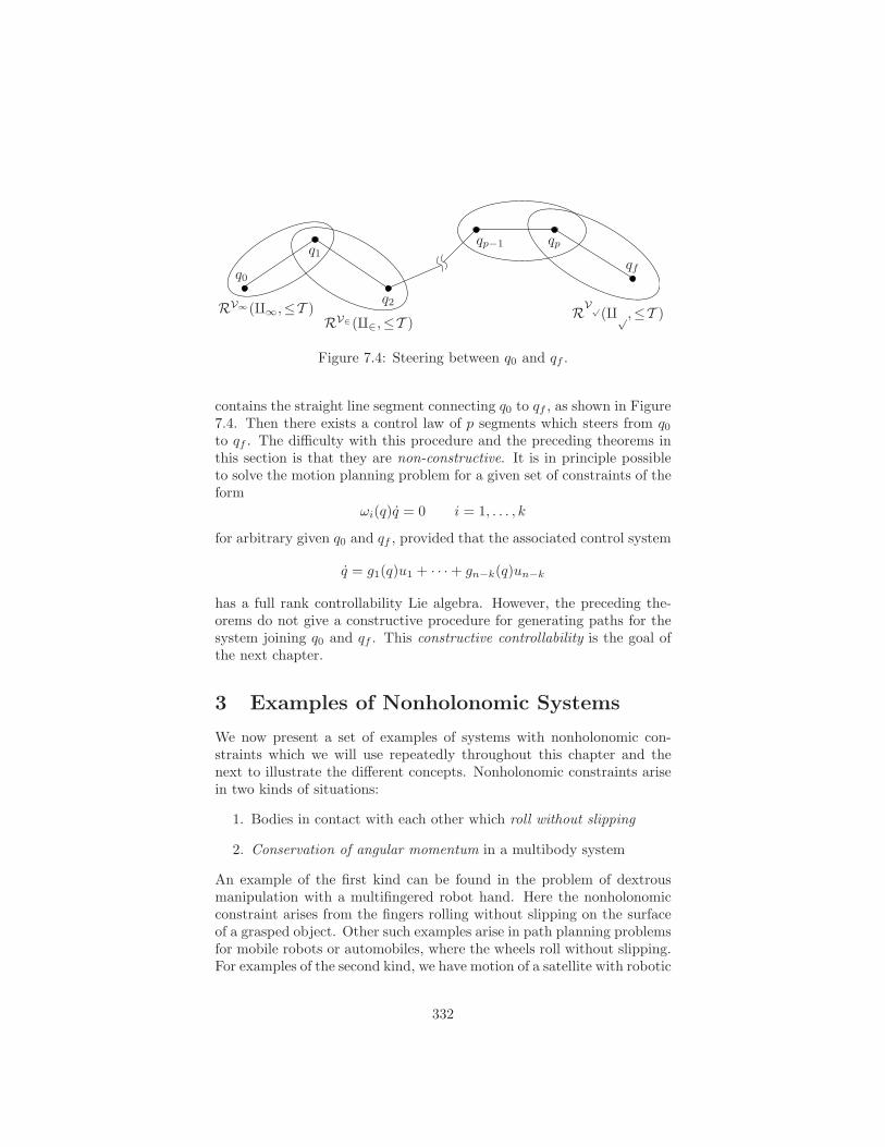
Figure 7.4: Steering between q0 and qf .

contains the straight line segment connecting q0 to qf , as shown in Figure7.4. Then there exists a control law of p segments which steers from q0

to qf . The di"culty with this procedure and the preceding theorems inthis section is that they are non-constructive. It is in principle possibleto solve the motion planning problem for a given set of constraints of theform

"i(q)q = 0 i = 1, . . . , k

for arbitrary given q0 and qf , provided that the associated control system

q = g1(q)u1 + · · · + gn!k(q)un!k

has a full rank controllability Lie algebra. However, the preceding the-orems do not give a constructive procedure for generating paths for thesystem joining q0 and qf . This constructive controllability is the goal ofthe next chapter.

3 Examples of Nonholonomic Systems

We now present a set of examples of systems with nonholonomic con-straints which we will use repeatedly throughout this chapter and thenext to illustrate the di!erent concepts. Nonholonomic constraints arisein two kinds of situations:

1. Bodies in contact with each other which roll without slipping

2. Conservation of angular momentum in a multibody system

An example of the first kind can be found in the problem of dextrousmanipulation with a multifingered robot hand. Here the nonholonomicconstraint arises from the fingers rolling without slipping on the surfaceof a grasped object. Other such examples arise in path planning problemsfor mobile robots or automobiles, where the wheels roll without slipping.For examples of the second kind, we have motion of a satellite with robotic

332

l

!

)

d

Figure 7.5: A simple hopping robot.

appendages moving in space, where angular momentum is conserved, ora diver or gymnast in mid-air maneuvers.

In the sequel, we will give a description of several nonholonomic sys-tems. The proof of their nonholonomy (that is the impossibility of findingfunctions of the configuration variables which are “integrals” of the con-straints) is deferred to Section 4.

Example 7.2. Hopping robot in flightAs our first example, we consider the dynamics of a hopping robot inthe flight phase, as shown in Figure 7.5. This robot consists of a bodywith an actuated leg that can rotate and extend; the “constraint” on thesystem is conservation of angular momentum.

The configuration q = (), l, !) consists of the leg angle, the leg exten-sion, and the body angle of the robot. We denote the moment of inertiaof the body by I and concentrate the mass of the leg, m, at the foot.The upper leg length is taken to be d, with l representing the extensionof the leg past this point. The total angular momentum of the robot isgiven by

I ! + m(l + d)2(! + )). (7.11)

Assume that the angular momentum of the robot is initially zero. Equa-tion (7.11) is a single Pfa"an constraint in the three velocities ), l, and !.Thus, the associated control system has two inputs—three configurationvariables minus one constraint. As a basis for the 2-dimensional rightnull space of the constraint, we choose one vector field corresponding tocontrolling the leg angle ), and the other corresponding to controlling

333

!

)2

)1

l

mr

Figure 7.6: A simplified model of a planar space robot.

the leg extension l; i.e., set ) = u1 and l = u2. Then, we have

g1(q) =

"

#$

10

" m(l+d)2

I+m(l+d)2

%

&' g2(q) =

"

$010

%

'

and the equivalent control system is given by

q = g1(q)u1 + g2(q)u2.

Example 7.3. Planar space robotFigure 7.6 shows a simplified model of a planar robot consisting of twoarms connected to a central body via revolute joints. If the robot is freefloating, then the law of conservation of angular momentum implies thatmoving the arms causes the central body to rotate. In the case thatthe angular momentum is zero, this conservation law can be viewed as aPfa"an constraint on the system.

Let M and I represent the mass and inertia of the central body andlet m represent the mass of the arms, which we take to be concentratedat the tips. The revolute joints are located a distance r from the middleof the central body and the links attached to these joints have lengthl. We let (x1, y1) and (x2, y2) represent the position of the ends of eachof the arms (in terms of !, )1, and )2). Assuming that the body isfree floating in space and that friction is negligible, we can derive theconstraints arising from conservation of angular momentum.

334

Let ! be the angle of the central body with respect to the horizontal,)1 and )2 the angles of the left arm and right arms with respect to thecentral body, and p ! R2 the location of a point on the central body (saythe center of mass). The kinetic energy of the system has the form

K =1

2(M + 2m).p.2 +

1

2I !2 +

1

2m(x2

1 + y21) +

1

2m(x2

2 + y22)

=1

2(M + 2m).p.2 +

1

2

"

$)1

)2

!

%

'

T "

$a11 a12 a13

a12 a22 a23

a13 a23 a33

%

'

"

$)1

)2

!

%

' ,

where aij can be calculated as

a11 = a22 = ml2

a12 = 0

a13 = ml2 + mr cos)1

a23 = ml2 + mr cos)2

a33 = I + 2ml2 + 2mr2 + 2mrl cos)1 + 2mrl cos)2.

Note that the kinetic energy of the system is independent of the variable!. It therefore follows from Lagrange’s equations that in the absence ofexternal forces,

d

dt

#L

#!=

#L

#!= 0.

Thus the quantity "L"%

is a constant of the motion. This is precisely theangular momentum, µ, of the system:

µ =#L

#!= a13)1 + a23)2 + a33!.

If the initial angular momentum is zero, then conservation of angularmomentum ensures that the angular momentum stays zero, giving thefollowing constraint equation

a13()))1 + a23()))2 + a33())! = 0. (7.12)

Since the variables that are actuated are the hinge angles of the leftand right arm, we choose as inputs u1 = )1 and u2 = )2. Using these inequation (7.12) and setting q = ()1,)2, !), we get

q = g1(q)u1 + g2(q)u2

where

g1(q) =

"

$10

!a13a33

%

' g2(q) =

"

$01

!a23a33

%

' .

335

!

%

(x, y)

Figure 7.7: Disk rolling on a plane.

Example 7.4. Disk rolling on a planeConsider the motion of a thin flat disk rolling on a plane shown in Fig-ure 7.7. The configuration space of the system is parameterized by thexy location of the contact point of the disk with the plane, the angle !that the disk makes with the horizontal line, and the angle % of a fixedline on the disk with respect to the vertical axis. We assume that thedisk rolls without slipping. As a consequence we have that

x " * cos ! % = 0

y " * sin ! % = 0,

where * > 0 is the radius of the disk. Writing these equations in the formof Pfa"an constraints with q = (x, y, !,%) we have

-1 0 0 "* cos !0 1 0 "* sin !

.q = 0.

Choosing ! = u1, the rate of rolling, and % = u2, the rate of turningabout the vertical axis, we have the associated control system:

q =

"

##$

* cos !* sin !

01

%

&&' u1 +

"

##$

0010

%

&&' u2. (7.13)

Example 7.5. Kinematic carConsider a simple kinematic model for an automobile with front and reartires, as shown in Figure 7.8. The rear tires are aligned with the car, whilethe front tires are allowed to spin about the vertical axes. To simplify thederivation, we model the front and rear pairs of wheels as single wheelsat the midpoints of the axles. The constraints on the system arise byallowing the wheels to roll and spin, but not slip.

Let (x, y, !,%) denote the configuration of the car, parameterized bythe xy location of the rear wheel(s), the angle of the car body with

336

y

x

l

%

!

Figure 7.8: Kinematic model of an automobile.

respect to the horizontal, !, and the steering angle with respect to thecar body, %. The constraints for the front and rear wheels are formedby setting the sideways velocity of the wheels to zero. In particular, thevelocity of the back wheels perpendicular to their direction is sin !x "cos !y and the velocity of the front wheels perpendicular to the directionthey are pointing is sin(!+%)x"cos(!+%)y"l! cos%, so that the Pfa"anconstraints on the automobile are:

sin(! + %)x " cos(! + %)y " l cos% ! = 0

sin ! x " cos ! y = 0.

Converting this to a control system with the inputs chosen as thedriving velocity u1 and the steering velocity u2 gives

"

##$

xy!%

%

&&' =

"

##$

cos !sin !

1l tan%

0

%

&&' u1 +

"

##$

0001

%

&&' u2. (7.14)

For this choice of vector fields, u1 corresponds to the forward velocity ofthe rear wheels of the car and u2 corresponds to the velocity of the angleof the steering wheel.

Example 7.6. Fingertip rolling on an objectLet us analyze the motion of a curved fingertip over a curved object. Aswe discussed in Section 6 of Chapter 5, we parameterize the object surfaceby $o ! R2, the fingertip surface by $f ! R2, and the angle of contactby ) ! S1, giving a 5-dimensional configuration space. The kinematic

337

equations of contact are given by

$f = M!1f (Kf + Ko)

!1

/-""y

"x

." Ko

-vx

vy

.0

$o = M!1o R&(Kf + Ko)

!1

/-""y

"x

.+ Kf

-vx

vy

.0

) = "z + TfMf $f + ToMo$o.

(7.15)

The rolling constraint is obtained by setting the sliding velocity and thevelocity of rotation about the contact normal to zero:

-vx

vy

.= 0 "z = 0. (7.16)

Substituting (7.16) into equation (7.15) yields the following constraints:

Mf $f " R&Mo$o = 0

TfMf $f + ToMo$o " ) = 0.(7.17)

If we set q = ($f ,$o,)) ! R5, then the foregoing set of three constraintsis of the form

"i(q)q = 0 i = 1, 2, 3.

To obtain a control system associated with these constraints, we let u1 ="x and u2 = "y in the kinematic equations for rolling contact. Afterrearranging the results, we have

q =

"

$M!1

f

M!1o R&

Tf + ToR&

%

' (Kf + Ko)!1

/-01

.u1 +

-"10

.u2

0. (7.18)

We now specialize the example to the case that the object is flatand the fingertip is a sphere of radius one. The curvature forms, metrictensors, and torsions for the fingertip and the object have been derivedin Example 5.7 and are reproduced here for convenience:

Ko =

-0 00 0

.Kf =

-1 00 1

.

Mo =

-1 00 1

.Mf =

-1 00 cos q1

.

To =(0 0

)Tf =

(0 " tan q1

).

Substituting the above results into (7.17) gives"

$1 0 " cos q5 sin q5 00 cos q1 sin q5 cos q5 00 sin q1 0 0 1

%

' q = 0.

338

In this case, the formula (7.18) gives, with the inputs being the rates ofrolling about the two tangential directions,

"

####$

q1

q2

q3

q4

q5

%

&&&&'

=

"

####$

0sec q1

" sin q5

" cos q5

" tan q1

%

&&&&'

u1 +

"

####$

"10

" cos q5

sin q5

0

%

&&&&'

u2. (7.19)

4 Structure of Nonholonomic Systems

We return to the problem of motion planning for systems satisfying linearvelocity constraints of the form

"i(q)q = 0 i = 1, . . . , k.

In Section 2 we showed how the problem of finding feasible trajectoriesin the configuration space could be dualized to one of finding trajectoriesof the control system

q = g1(q)u1 + · · · + gm(q)um, (7.20)

with m = n " k and "i(q)gj(q) = 0. From the controllability rankcondition, it follows that one can find a trajectory joining an arbitrarystarting point and end point if the rank of the Lie algebra generated byg1, . . . , gm is n. If #q ,= TqRn and in addition #q has a constant rankn " p which is less than n, then it follows from Frobenius’ theorem thatthere exist functions hi(q) = ci, i = 1, . . . , p such that

"i(q)q = 0 i = 1, . . . , k $% hj(q) = cj j = 1, . . . , p.

Consider this a little further: since the dimension of # is greater thanor equal to the dimension of #, it follows that p & k. Thus, the num-ber of functions whose level sets are tangential to the given distributionare fewer than the dimension of the distribution. The process of con-verting from the given constraints, specified as a codistribution, to anequivalent control system and then integrating the involutive closure ofthis distribution may seem to be convoluted. It is indeed possible to dealdirectly with a given codistribution and to find the maximal integrablecodistribution contained within it, but this involves methods of exteriordi!erential systems which are beyond the scope of this book. Of course,in the event that # = TqRn for all q, then p = 0, i.e., there are no non-trivial functions which integrate the given constraints. In this case thedistribution is said to be completely nonholonomic, as was noted earlier.

In this section, we will try to make precise some notation that we willuse in dealing with nonholonomic systems and apply it to the examples

339

that we considered in Section 3. Some additional machinery to study thegrowth of the controllability Lie algebra is discussed at the end of thissection.

4.1 Classification of nonholonomic distributions

The complexity of the motion planning problem is related to the or-der of Lie brackets in its controllability Lie algebra. Here we developsome concepts which allow us to classify nonholonomic systems. Let# = span{g1, . . . , gm} be the distribution associated with the controlsystem (7.20). Define #1 = # and

#i = #i!1 + [#1,#i!1],

where[#1,#i!1] = span{[g, h] : g ! #1, h ! #i!1}.

It is clear that #i ' #i+1. The chain of the distributions #i is definedas the filtration associated with the distribution # = #1. Each #i isdefined to be spanned by the input vector fields plus the vector fieldsformed by taking up to i" 1 Lie brackets of the generators, i.e., elementsof #1. The Jacobi identity (see Proposition 7.1, page 325) implies that[#i,#j ] ' [#1,#i+j!1] ' #i+j . The proof of this fact is left as anexercise.

A filtration is said to be regular in a neighborhood U of q0 if

rank #i(q) = rank #i(q0) )q ! U.

We say the control system (7.20) is regular if the corresponding filtrationis regular. If a filtration is regular, then at each step of its construction,#i

either gains dimension or#i+1 = #i, so that the construction terminates.If rank #i+1 = rank #i, then #i is involutive and hence #i+j = #i forall j / 0. Clearly, rank #i & n and hence if a filtration is regular, thenthere exists an integer + <n such that #i = #' for all i / +.

Definition 7.2. Degree of nonholonomyConsider a regular filtration {#i} associated with a distribution #. Thesmallest integer + such that the rank of #' is equal to that of #'+1 iscalled the degree of nonholonomy of the distribution.

We know that rank #' & n. In general, let the rank of #' = n " p.Then, by Frobenius’ theorem there are p functions hi for i = 1, . . . , pwhose level surfaces are the integral manifolds of #'. Thus, the state qof the control system must be confined to the a level set of the hi’s. This,then, is the complete answer to the question we posed ourselves at thebeginning of this chapter. The maximum number of functions hi suchthat

span{#h1

#q, . . . ,

#hp

#q} ' span{"1, . . . ,"k}

340

is given to be the set of functions such that

span{#h1

#q, . . . ,

#hp

#q} = (#)%

by Frobenius’ theorem. If p = 0, that is rank #' is equal to n, thenthere are no nontrivial functions hi and it is possible to steer betweenarbitrary given initial and final points. This is Chow’s theorem, whichwas discussed in the previous section. Chow’s theorem is actually alsovalid when the filtration #i is not regular, as long as # is smooth andconstant rank.

We now give a definition which serves to classify the growth of afiltration:

Definition 7.3. Growth vector, relative growth vectorConsider a regular filtration associated with a given distribution # andhaving degree of nonholonomy +. For such a system, we define the growthvector r ! Z' as

ri = rank #i.

We define the relative growth vector , ! Z' as ,i = ri " ri!1 and r0 := 0.

The growth vector for a regular filtration is a convenient way to rep-resent complexity information about the associated controllability Liealgebra.

4.2 Examples of nonholonomic systems, continued

In this subsection, we illustrate the classification of nonholonomic systemson the examples that were developed in Section 3.

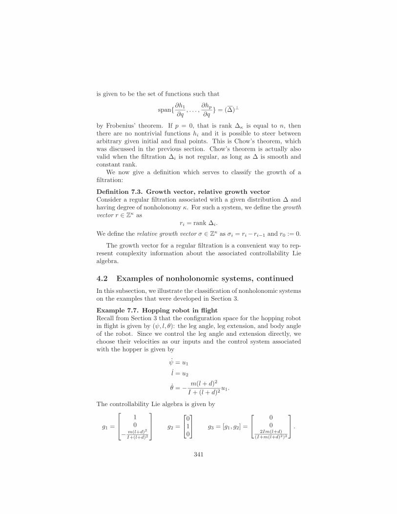
Example 7.7. Hopping robot in flightRecall from Section 3 that the configuration space for the hopping robotin flight is given by (), l, !): the leg angle, leg extension, and body angleof the robot. Since we control the leg angle and extension directly, wechoose their velocities as our inputs and the control system associatedwith the hopper is given by

) = u1

l = u2

! = " m(l + d)2

I + (l + d)2u1.

The controllability Lie algebra is given by

g1 =

"

#$

10

" m(l+d)2

I+(l+d)2

%

&' g2 =

"

$010

%

' g3 = [g1, g2] =

"

$00

2Im(l+d)(I+m(l+d)2)2

%

' .

341

In a neighborhood of l = 0, span{g1, g2, g3} is full rank and hence thehopping robot has degree of nonholonomy 2 with growth vector (2, 3) andrelative growth vector (2, 1).

Example 7.8. Planar space robotFrom Example 7.3, we have that the angular momentum conservationconstraint yields

a13())!1 + a23())!2 + a33())! = 0,

where the vector of configuration variables is q = ()1,)2, !). Using thecontrol equations derived in Example 7.3, we have

g1 =

"

$10

" ml2+mr cos&1

I+2ml2+2mr2+2mrl cos&1+2mrl cos&2

%

'

g2 =

"

$10

" ml2+mr cos&2

I+2ml2+2mr2+2mrl cos&1+2mrl cos&2

%

'

and the Lie bracket is

g3 = [g1, g2] =

"

#$

00

2m2l2r(!l sin&1!r sin(&1!&2)+l sin&2)(I+2ml2+2mr2+2mlr cos&1+2mlr cos&2)2

%

&' .

The vector field g3 is zero when )1 = )2 and hence the filtration {#i}is not regular. By computing higher order Lie brackets, however, it ispossible to show that #q = TqR3 in a neighborhood of q = 0 and thesystem is controllable.

Example 7.9. Disk rolling on a planeFrom Example 7.4, the control system which describes a disk rolling ona plane is described by the distribution spanned by

g1 =

"

##$

* cos !* sin !

01

%

&&' g2 =

"

##$

0010

%

&&' .

The control Lie algebra is constructed by computing the following vectorfields:

g3 = [g1, g2] =

"

##$

* sin !"* cos !

00

%

&&' g4 = [g2, g3] =

"

##$

* cos !* sin !

00

%

&&' .

342

For all q, span{g1, g2, g3, g4} is full rank and hence the rolling disk hasdegree of nonholonomy 3 with growth vector (2, 3, 4). The relative growthvector for this system is (2, 1, 1).

Example 7.10. Kinematic carRecall that (x, y, !,%) denotes the configuration of the car, parameterizedby the location of the rear wheel(s), the angle of the car body with respectto the horizontal, and the steering angle with respect to the car body.The constraints for the front and rear wheels to roll without slipping aregiven by the following equations:

sin(! + %)x " cos(! + %)y " l cos% ! = 0

sin ! x " cos ! y = 0.

Converting this to a control system with the driving and steering velocityas inputs gives the control system of equation (7.14).

To calculate the growth vector, we build the filtration

g1 =

"

##$

cos !sin !

1l tan%

0

%

&&' g2 =

"

##$

0001

%

&&'

g3 = [g1, g2] =

"

##$

00

" 1l cos2 (

0

%

&&' g4 = [g1, g3] =

"

##$

" sin %l cos2 (cos %cos2 (

00

%

&&' .

The vector fields {g1, g2, g3, g4} are linearly independent when % ,= ±-.Thus the system has degree of nonholonomy 3 with growth vector r =(2, 3, 4) and relative growth vector , = (2, 1, 1). The system is regularaway from % = ±-/2, at which point g1 is undefined.

Example 7.11. Spherical finger rolling on a planeLet the inputs be the two components of rolling velocities, i.e., u1 = "x

and u2 = "y. The associated control system is derived in (7.19), whichin vector field form reads

g1 =

"

####$

0sec q1

" sin q5

" cos q5

" tan q1

%

&&&&'

g2 =

"

####$

"10

" cos q5

sin q5

0

%

&&&&'

.

343

Constructing the filtration, we have

g3 = [g1, g2] =

"

####$

0tan q1 sec q1

" tan q1 sin q5

" tan q1 cos q5

" sec2 q1

%

&&&&'

g4 = [g1, g3] =

"

####$

00

" cos q5

sin q5

0

%

&&&&'

g5 = [g2, g3] =

"

####$

0"(1 + sin2 q1) sec3 q1

2 sin q5 sec2 q1

2 cos q5 sec2 q1

2 tan q1 sec2 q1

%

&&&&'

.

In a neighborhood of q = 0 (more specifically in a neighborhood notcontaining q1 = )

2 ) the vector fields {g1, g2, g3, g4, g5} are linearly inde-pendent, thus establishing that the degree of nonholonomy is 3 and thatthe growth vector is (2, 3, 5). The relative growth vector is (2, 1, 2).

4.3 Philip Hall basis

Let L(}", . . . , }#) be the Lie algebra generated by a set of vector fieldsg1, . . . , gm. One approach to equipping L(}", . . . , }#) with a basis is tolist all the generators and all of their Lie products. The problem is thatnot all Lie products are linearly independent because of skew-symmetryand the Jacobi identity. The Philip Hall basis is a particular way to selecta basis which takes into account skew-symmetry and the Jacobi identity.

Given a set of generators {g1, · · · , gm}, we define the length of a Lieproduct recursively as

l(gi) = 1 i = 1, · · · ,m

l([A,B]) = l(A) + l(B),

where A and B are themselves Lie products. Alternatively, l(A) is thenumber of generators in the expansion for A. A Lie algebra is nilpotentif there exists an integer k such that all Lie products of length greaterthan k are zero. The integer k is called the order of nilpotency.

A Philip Hall basis is an ordered set of Lie products H = {Bi} satis-fying:

1. gi ! H, i = 1, . . . ,m

2. If l(Bi) < l(Bj) then Bi < Bj

3. [Bi, Bj ] ! H if and only if

(a) Bi, Bj ! H and Bi < Bj and

344

(b) either Bj = gk for some k or Bj = [Bl, Br] with Bl, Br ! Hand Bl & Bi.

The proof that a Philip Hall basis is indeed a basis for the Lie algebragenerated by {g1, . . . , gm} is beyond the scope of this book and may befound in [38] and [104]. A Philip Hall basis which is nilpotent of orderk can be constructed from a set of generators using this definition. Thesimplest approach is to construct all possible Lie products with lengthless than k and use the definition to eliminate elements which fail tosatisfy one of the properties. In practice, the basis can be built in such away that only condition 3 need be checked.

Example 7.12. Philip Hall basis of order 3A basis for the nilpotent Lie algebra of order 3 generated by g1, g2, g3 is

g1 g2 g3

[g1, g2] [g2, g3] [g3, g1][g1, [g1, g2]] [g1, [g1, g3]] [g2, [g1, g2]] [g2, [g1, g3]][g2, [g2, g3]] [g3, [g1, g2]] [g3, [g1, g3]] [g3, [g2, g3]]

Note that [g1, [g2, g3]] does not appear since

[g1, [g2, g3]] + [g2, [g3, g1]] + [g3, [g1, g2]] = 0

by the Jacobi identity and the second two terms in the formula are alreadypresent.

345

5 Summary

The following are the key concepts covered in this chapter:

1. Nonholonomic constraints are linear velocity constraints of the form

"i(q)q = 0 i = 1, . . . , k

which cannot be integrated to give constraints on the configurationvariables q alone. By choosing gj(q), j = 1, . . . , n " k =: m to bea basis for the null space of the linear velocity constraints, we getthe associated control system

q = g1(q)u1 + · · · + gm(q)um.

The problem of nonholonomic motion planning consists of findinga trajectory q(·) : [0, T ] # Rn, given q(0) = q0 and q(T ) = qf .

2. The Lie bracket between two vector fields f and g on Rn is a newvector field [f, g] defined by

[f, g](q) =#g

#qf(q) " #f

#qg(q).

3. A distribution# is a smooth assignment of a subspace of the tangentspace to each point q ! Rn. One important way of generating it isas the span of a number of vector fields:

# = span{g1, . . . , gm}.

The distribution # is said to be regular if the dimension of #q doesnot vary with q. The distribution # is said to be involutive if itis closed under the Lie bracket, that is if for all f, g ! #, we have[f, g] ! #.

4. A distribution # of dimension k is said to be integrable if thereexist n" k independent functions whose di!erentials annihilate thedistribution. Frobenius’ theorem asserts that a regular distributionis integrable if and only if it is involutive. A Pfa"an system orcodistribution $

$ = span{"1, . . . ,"k}

is completely nonholonomic if the involutive closure of the distribu-tion # = $% spans Rn for all q.

5. Consider the system

q = g1(q)u1 + · · · + gm(q)um.

346

The controllability Lie algebra is the Lie algebra generated by thevector fields g1, . . . , gm. It is the smallest Lie algebra containingg1, . . . , gm. Chow’s theorem asserts that if the controllability Liealgebra is full rank, we can steer this system from any initial to anyfinal point.

6. Given a distribution #, the filtration associated with # is definedby #1 = # and

#i = #i!1 + [#1,#i!1],

where[#1,#i!1] = span{[g, h] : g ! #1, h ! #i!1}.

The filtration is said to be regular if each of the #i are regular. Fora regular filtration, the smallest integer + at which rank #' is equalto that of #'+1,#'+2, . . . is called the degree of nonholonomy ofthe distribution. The growth vector r ! Z' for a regular filtrationis defined as ri := rank #i. The relative growth vector , ! Z' isdefined as ,i = ri " ri!1 with r0 = 0.

7. Given # = span{g1, . . . , gm}, a Lie product is any nested set of Liebrackets of the generators gi. A Lie algebra generated by # is saidto be nilpotent if there exists an integer k such that all Lie productsof length greater than k are zero. A Philip Hall basis is an orderedset of Lie products chosen by a set of rules so as to keep track of therestrictions imposed by the properties of the Lie bracket, namelyskew-symmetry and the Jacobi identity.

6 Bibliography

The topic of holonomy and nonholonomy of Pfa"an constraints has cap-tured the attention of many of the earliest writers on classical mechan-ics. A nice description of the mechanics point of view is given in [81].Chapter 1 of Rosenberg [99] makes mention of the di!erent kinds of con-straints: holonomic, rheonomic, scleronomic. The examples in this chap-ter are drawn from our interest in fingers rolling on the surface of anobject [60, 76], mobile robots and parking problems [78, 112], and spacerobots [119, 32]. A recent collection of papers on nonholonomic motionplanning is [61].

Work on nonlinear controllability has a long history as well, withrecognition of the connections between Chow’s theorem and controlla-bility in Hermann and Krener [40]. Good textbook presentations of thework on nonlinear control are available in [43], and [83]. The theory ofnonholonomic distributions presented here was originally developed byVershik and Gershkovic [117]. The notation we follow is theirs and ispresented in [78].

347

A somewhat less obvious application of the methods of this chapter isin the analysis of control algorithms for redundant manipulators. In thisapplication, one looks for an algorithm such that closed trajectories of theend-e!ector generate closed paths in the joint space of the manipulator.This is closely related to the integrability of a set of constraints. A gooddescription of this is in the work of Shamir and Yomdin [105], Baillieuland Martin [5], Chiacchio and Siciliano [17], and De Luca and Oriolo [23].

348

7 Exercises

1. Show that the controllability rank condition is also a necessary con-dition for local controllability under the usual smoothness and reg-ularity assumptions.

2. Show that the di!erential constraint in R5 given by

(0 1 * sin q5 * cos q3 cos q5

)q = 0

is nonholonomic.

3. Use the definition of the Lie bracket to prove the properties listedin Proposition 7.1.

4. Consider the system %,

q = g1(q)u1 + · · · + gm(q)um.

Let u : [0, T ] # Rm be input which steers % from q0 to qf in Tunits of time.

(a) Show that the input u : [0, 1] # Rm defined by

u(t) = u(t/T )

steers , from q0 to qf in 1 unit of time.

(b) Show that the input u : [0, 1] "# Rm defined by

u(t) = "u(1 " t)

steers , from qf to q0 in 1 unit of time.

5. Spheres rolling on spheresDerive the control equation for a unit sphere in rolling contact withanother sphere of radius * with the same inputs as in Example 7.6.Show that the system is controllable if and only if * ,= 1.

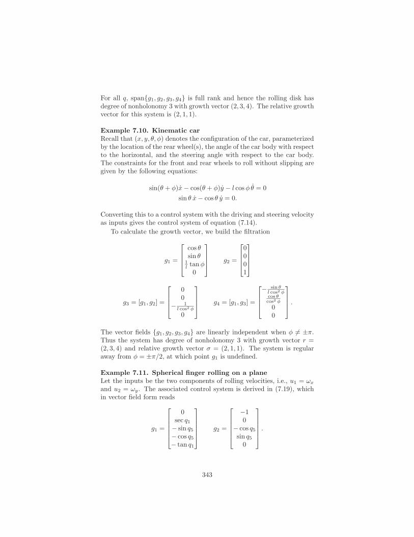
6. Car with N trailersThe figure below shows a car with N trailers attached. We attachthe hitch of each trailer to the center of the rear axle of the previoustrailer. The wheels of the individual trailers are aligned with thebody of the trailer. The constraints are again based on allowingthe wheels only to roll and spin, but not slip. The dimension of thestate space is N + 4 with 2 controls.

349

!N

y

x

!0

!1

%

l

Parameterize the configuration by the states of the automobile plusthe angle of each of the trailers with respect to the horizontal. Showthat the control equation for the system has the form

x = cos !0 u1

y = sin !0 u1

% = u2

!0 =1

ltan%u1

!i =1

di

1

2i!13

j=1

cos(!j!1 " !j)

4

5 sin(!i!1 " !i)u1.

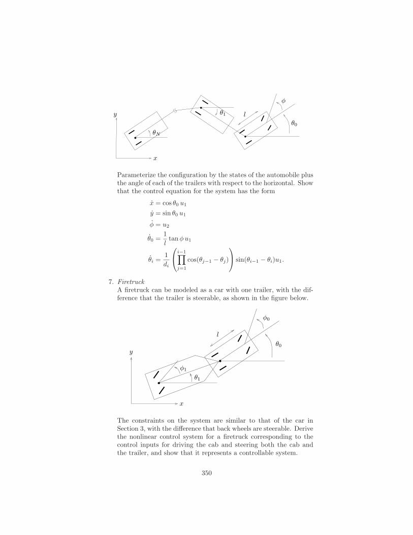
7. FiretruckA firetruck can be modeled as a car with one trailer, with the dif-ference that the trailer is steerable, as shown in the figure below.

!0

x

y

l

!1

%1

%0

The constraints on the system are similar to that of the car inSection 3, with the di!erence that back wheels are steerable. Derivethe nonlinear control system for a firetruck corresponding to thecontrol inputs for driving the cab and steering both the cab andthe trailer, and show that it represents a controllable system.

350

8. Prove that a 1-dimensional distribution #q = span{f(q)} is invo-lutive. More specifically, show that for any two smooth functions $and '

[$f,'f ] ! #.

9. Prove that the two definitions of Lie bracket given in this chapter,namely,

[f, g] =#g

#qf " #f

#qg,

andL[f,g]$ = Lf (Lg$) " Lg(Lf$) )$ : Rn # R,

are equivalent.

10. Use induction and Jacobi’s identity to prove that

[#i,#j ] ' [#1,#i+j!1] ' #i+j ,

where # = #1 ' #2 ' · · · is a filtration associated with a distri-bution 0.

11. Let #i, i = 1, . . . ,+ be a regular filtration associated with a distri-bution. Show that if rank(#i+1) = rank(#i) then #i is involutive.(Hint: use Exercise 10).

12. Satellite with 2 rotorsFigure 7.9 shows a model of a satellite body with two symmetricallyattached rotors, where the rotors’ axes of rotation intersect at apoint. The constraint on the system is conservation of angularmomentum.

(a) Assuming that the initial angular momentum of the system iszero, show that the (body) angular velocity, "1, of the satellitebody is related to the rotor velocities (u1, u2) by

"1 = b1u1 + b2u2 (7.21)

where b1, b2 ! R3 are constant vectors.

Equation (7.21) gives rise to a di!erential equation in the ro-tation group SO(3) for the satellite body

R(t) = R(t)(6b1u1 +6b2u2). (7.22)

(b) Obtain a local coordinate description of (7.22) using the Eu-ler parameters of SO(3) (from Chapter 2) and show that theresulting system is controllable.

351

rotor

Inertia frame

framebody

rotor

Figure 7.9: A model of a satellite body with two rotors. The satellitecan be repositioned by controlling the rotor velocities. (Figure courtesyof Greg Walsh)

13. The figure below shows a simplified model of a falling cat. It consistsof two pendulums coupled by a spherical joint. The configurationspace of the system is Q = S2 * S2, where S2 is the unit sphere inR3.

mm

dd

(a) Derive the Pfa"an constraints arising from conservation of an-gular momentum and dualize the results to obtain the controlsystem for nonholonomic motion planning.

(b) Is the system in part (a) controllable?

14. Write a computer program to write a Philip Hall basis of given orderfor a set of m generators g1, . . . , gm. Use your program to generatea Philip Hall basis of order 5 for a system with 2 generators.

352

15. Consider the system of Exercise 6. Write a computer program (oruse Mathematica or any other symbolic manipulation software pack-ages) to compute the filtration associated with the system. Showthat the system is controllable, with degree of nonholonomy N + 2and relative growth vector (2, 1, . . . , 1).

16. In this chapter, we restricted ourselves to constraints of the form

"i(q)q = 0 i = 1, . . . , k.

Consider what would happen if the constraints were of the form

"i(q)q = ci i = 1, . . . , k

for constants ci. Dualize these constraints to get an associatedcontrol system of the form

q = f(q) +n!k!

i=1

gi(q)ui.

What is the formula for f(q)? Apply this method to the spacerobot with nonzero angular momentum. What di"culties wouldone encounter in path planning for these examples? These systemsare called systems with drift.

17. (Hard) Show that for a regular system the growth vector is boundedabove by

,i =1

i

1

2(,1)i "

!

j|i, j<i

j,j

4

5 i > 1,

where ,i is the maximum relative growth at the ith stage and j|imeans all integers j such that j divides i. If ,i = ,i for all i, wesay that the system has maximum growth.

353

354