nondeterministic turing machines - university of...
TRANSCRIPT

Nondeterministic Turing MachinesRemarks.
I The complexity class P consists of all decision problems that can be solved by adeterministic Turing machine in polynomial time.
I The complexity class NP consists of all decision problems that can be solved by anon-deterministic Turing machine in polynomial time.
I Guess a solution and check in polynomial time.I NP stands for Non-deterministic Polynomial.
Lemma 8.2.P ✓ NP .
NP P
Proof: Deterministic Turing machines are a special case of non-deterministic Turingmachines.
208

Polynomial Transformations/Reductions
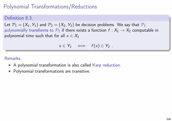
Definition 8.3.Let P1 = (X1,Y1) and P2 = (X2,Y2) be decision problems. We say that P1polynomially transforms to P2 if there exists a function f : X1 ! X2 computable inpolynomial time such that for all x 2 X1
x 2 Y1 () f (x) 2 Y2 .
Remarks.I A polynomial transformation is also called Karp reduction.I Polynomial transformations are transitive.
Lemma 8.4.Let P1 and P2 be decision problems. If P2 2 P and P1 polynomially transforms to P2,then P1 2 P .
209
Polynomial Transformations/Reductions
Definition 8.3.Let P1 = (X1,Y1) and P2 = (X2,Y2) be decision problems. We say that P1polynomially transforms to P2 if there exists a function f : X1 ! X2 computable inpolynomial time such that for all x 2 X1
x 2 Y1 () f (x) 2 Y2 .
Remarks.I A polynomial transformation is also called Karp reduction.I Polynomial transformations are transitive.
Lemma 8.4.Let P1 and P2 be decision problems. If P2 2 P and P1 polynomially transforms to P2,then P1 2 P .
209

NP-Hardness and NP-Completeness
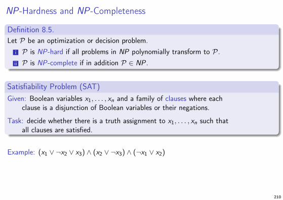
Definition 8.5.Let P be an optimization or decision problem.
i P is NP-hard if all problems in NP polynomially transform to P.ii P is NP-complete if in addition P 2 NP .
Satisfiability Problem (SAT)Given: Boolean variables x1, . . . , xn and a family of clauses where each
clause is a disjunction of Boolean variables or their negations.
Task: decide whether there is a truth assignment to x1, . . . , xn such thatall clauses are satisfied.
Example: (x1 _ ¬x2 _ x3) ^ (x2 _ ¬x3) ^ (¬x1 _ x2)
210

NP-Hardness and NP-Completeness
Definition 8.5.Let P be an optimization or decision problem.
i P is NP-hard if all problems in NP polynomially transform to P.ii P is NP-complete if in addition P 2 NP .
Satisfiability Problem (SAT)Given: Boolean variables x1, . . . , xn and a family of clauses where each
clause is a disjunction of Boolean variables or their negations.
Task: decide whether there is a truth assignment to x1, . . . , xn such thatall clauses are satisfied.
Example: (x1 _ ¬x2 _ x3) ^ (x2 _ ¬x3) ^ (¬x1 _ x2)
210
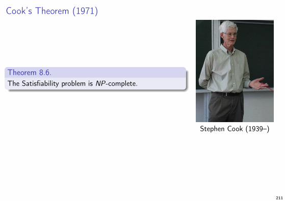
Cook’s Theorem (1971)
Theorem 8.6.The Satisfiability problem is NP-complete.
Stephen Cook (1939–)
Proof idea: SAT is obviously in NP . One can show that any non- deterministic Turingmachine can be encoded as an instance of SAT.
211

Cook’s Theorem (1971)
Theorem 8.6.The Satisfiability problem is NP-complete.
Stephen Cook (1939–)
Proof idea: SAT is obviously in NP . One can show that any non- deterministic Turingmachine can be encoded as an instance of SAT.
211
Proving NP-Completeness
Lemma 8.7.Let P1 and P2 be decision problems. If P1 is NP-complete, P2 2 NP , and P1polynomially transforms to P2, then P2 is NP-complete.
Proof: As mentioned above, polynomial transformations are transitive.
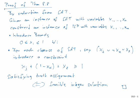
Integer Linear Programming Problem (ILP)Given: matrix A 2 Zm⇥n, vector b 2 Zm.
Task: decide whether there is x 2 Zn with A · x � b.
Theorem 8.8.ILP is NP-complete.
212

Proving NP-Completeness
Lemma 8.7.Let P1 and P2 be decision problems. If P1 is NP-complete, P2 2 NP , and P1polynomially transforms to P2, then P2 is NP-complete.
Proof: As mentioned above, polynomial transformations are transitive.
Integer Linear Programming Problem (ILP)Given: matrix A 2 Zm⇥n, vector b 2 Zm.
Task: decide whether there is x 2 Zn with A · x � b.
Theorem 8.8.ILP is NP-complete.
212
212 - 1

212 - 2
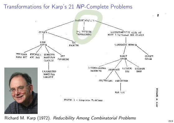
Transformations for Karp’s 21 NP-Complete Problems
Richard M. Karp (1972). Reducibility Among Combinatorial Problems213
P vs. NP
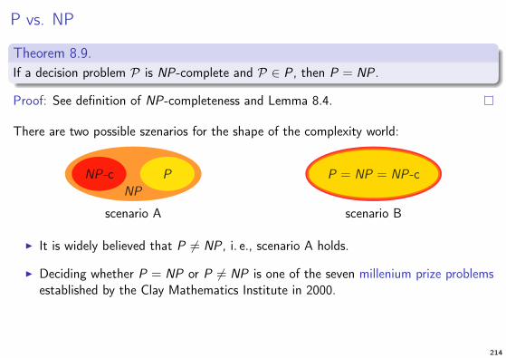
Theorem 8.9.If a decision problem P is NP-complete and P 2 P , then P = NP .
Proof: See definition of NP-completeness and Lemma 8.4.
There are two possible szenarios for the shape of the complexity world:
NP
PNP-c
scenario A
P = NP = NP-c
scenario B
I It is widely believed that P 6= NP , i. e., scenario A holds.
I Deciding whether P = NP or P 6= NP is one of the seven millenium prize problemsestablished by the Clay Mathematics Institute in 2000.
214

P vs. NP
Theorem 8.9.If a decision problem P is NP-complete and P 2 P , then P = NP .
Proof: See definition of NP-completeness and Lemma 8.4.
There are two possible szenarios for the shape of the complexity world:
NP
PNP-c
scenario A
P = NP = NP-c
scenario B
I It is widely believed that P 6= NP , i. e., scenario A holds.
I Deciding whether P = NP or P 6= NP is one of the seven millenium prize problemsestablished by the Clay Mathematics Institute in 2000.
214

215
Complexity of Linear Programming
I As discussed in Chapter 4, so far no variant of the simplex method has been shownto have a polynomial running time.
I Therefore, the complexity of Linear Programming remained unresolved for a longtime.
I Only in 1979, the Soviet mathematician Leonid Khachiyan proved that theso-called ellipsoid method earlier developed for nonlinear optimization can bemodified in order to solve LPs in polynomial time.
I In November 1979, the New York Times featured Khachiyan and his algorithm in afront-page story.
I Details can, e. g., be found in the book of Bertsimas & Tsitsiklis (Chapter 8) or inthe book Geometric Algorithms and Combinatorial Optimization by Grötschel,Lovász & Schrijver (Springer, 1988).
216
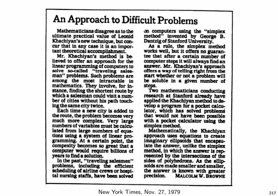
New York Times, Nov. 27, 1979 217

218