Non-Standard Rates of Convergence of

Criterion-Function-Based Set Estimators∗

JASON R. BLEVINS

The Ohio State University, Department of Economics

Working Paper 13-02

December 19, 2013†

Abstract. This paper establishes conditions for consistency and potentially non-standard

rates of convergence for set estimators based on contour sets of criterion functions. These

conditions cover the standard parametric rate n−1/2, non-standard polynomial rates such as

n−1/3, and an extreme case of arbitrarily fast convergence. We also establish the validity of a

subsampling procedure for constructing confidence sets for the identified set. We then provide

more convenient sufficient conditions on the underlying empirical processes for cube root

convergence. We show that these conditions apply to a class of transformation models under

weak semiparametric assumptions which may be partially identified due to potentially limited-

support regressors. We focus in particular on a semiparametric binary response model under a

conditional median restriction and show that a set estimator analogous to the maximum score

estimator is essentially cube-root consistent for the identified set when a continuous but possi-

bly bounded regressor is present. Arbitrarily fast convergence occurs when all regressors are

discrete. Finally, we carry out a series of Monte Carlo experiments which verify our theoretical

findings and shed light on the finite sample performance of the proposed procedures.

Keywords: partial identification, cube-root asymptotics, semiparametric models, limited sup-

port regressors, transformation model, binary response model, maximum score estimator.

JEL Classification: C13, C14, C25.

∗This paper is based in part on Chapter 2 of my Duke University dissertation. I am grateful to the members of

my committee, Han Hong, Shakeeb Khan, Paul Ellickson, and Andrew Sweeting, for their guidance and support.

I also thank Arie Beresteanu, Federico Bugni, Stephen Cosslett, Yanqin Fan, Joseph Hotz, Robert de Jong, Joris

Pinkse, Jean-François Richard, Xiaoxia Shi, Elie Tamer, and Jörg Stoye for helpful discussions and comments, and

seminar participants at Duke University, Ohio State University, the University of Illinois at Urbana-Champaign, the

University of Pittsburgh, the University of Texas at Austin, Vanderbilt University, the 2009 Triangle Econometrics

Conference and the 2010 Annual Meeting of the Midwest Econometrics Group for useful comments.†This paper is a revision of a working paper whose first draft appeared on October 31, 2011.

1

1. Introduction

Relaxing distributional assumptions in econometric models is often desirable but can lead to a

failure of point identification. Fortunately, a recent and growing literature on partially identified

models has shown that in many cases we can still carry out inference about the parameters of

interest even under assumptions weaker than those known to provide point identification.1 In

particular, a criterion-function-based approach to set estimation, which has close parallels to

classical extremum estimation, has proven useful for analyzing moment equality and inequality

models. Set estimators for this class of models, under certain regularity conditions, are essentiallypn-consistent (Chernozhukov, Hong, and Tamer, 2007).

However, many interesting econometric models fall outside of this class or do not satisfy the

regularity conditions. This includes transformation models under weak semiparametric assump-

tions such as the semiparametric binary response model we discuss in detail below. As such,

this paper develops the asymptotic properties of criterion-function-based set estimators and a

subsampling-based method for obtaining confidence sets in a new class of models containing

those cases of interest. Of particular interest is a set estimator analogous to the maximum score

estimator of Manski (1975, 1985). Kim and Pollard (1990) showed that the point estimator is

cube-root-consistent and has a non-standard limiting distribution. These properties are often

perceived as disadvantages, but the maximum score estimator has proven to be important and

useful due to its robustness, both to unknown error distributions and to heteroskedasticity of

unknown form. Furthermore, recent work on classical MCMC-based inference by Jun, Pinkse,

and Wan (2011) makes point estimation and inference for this model much more accessible.

The first primary contribution of this paper is to extend the criterion-function-based set

estimation approach to cases for which non-standard rates of convergence may arise. Work on

criterion-function-based estimation and inference in partially identified models started with

Manski and Tamer (2002), who analyzed a semiparametric binary response model with interval-

valued data under a conditional quantile restriction. They derived the sharp identified set for the

model, proposed a set estimator, defined as an appropriately-chosen contour set of a modified

maximum score objective function, and showed that it was consistent. Chernozhukov, Hong,

and Tamer (2007) developed a broad framework for criterion-function-based estimation and

established general conditions for consistency and rates of convergence of estimators in this

class. They also proposed a subsampling-based procedure for obtaining confidence sets with

some pre-specified coverage probability. Subsampling-based inference was further explored

by Romano and Shaikh (2008, 2010) and Andrews and Guggenberger (2009) while Bugni (2010)

and Canay (2010) have proposed bootstrap procedures. These and many other authors have

1See Manski (2003) and Tamer (2010) and the references therein for broad surveys of this literature.

2

studied inference in moment equality and inequality models, including but certainly not limited

to Andrews, Berry, and Jia (2004), Pakes, Porter, Ho, and Ishii (2006), Beresteanu and Molinari

(2008), Beresteanu, Molchanov, and Molinari (2011), Imbens and Manski (2004), Stoye (2009),

Kim (2008), Khan and Tamer (2009), Menzel (2008), Andrews and Shi (2013), Andrews and Soares

(2010), and Yildiz (2012).

We work under modifications of the conditions of Chernozhukov, Hong, and Tamer (2007) in

order to analyze and perform inference in the non-standard models we consider. A mechanism

analogous to Kim and Pollard’s “sharp-edge effect” is shown to drive cube-root convergence of

set estimators in a class of partially identified models. We also characterize a class of models

in which a natural discontinuity in the limiting objective function results in arbitrarily fast

convergence. We then verify that a subsampling procedure can be used for inference in these

cases. We also derive sufficient conditions for consistency, cube root convergence, and arbitrarily

fast convergence that are easier to verify in some cases, as we illustrate later in the context of a

binary response model.

Our second main contribution is to apply our general results to study identification and

estimation of a semiparametric binary response model under conditional median independence.

Even though the assumptions of the standard maximum score model are already weak, it may

be desirable to relax them even further for additional robustness. Known conditions for point

identification require at least one regressor to be continuous and have sufficiently rich support

(Manski, 1988; Horowitz, 1998). Furthermore, when additional smoothness conditions on the

distributions of the error term and the explanatory variables are satisfied, one can estimate the

parameters at a faster rate, approaching the parametric rate, using the smoothed maximum score

estimator (Horowitz, 1992). However, when the regressors are discrete or bounded, the model

may only be partially identified. Therefore, we propose a set estimator that is closely analogous

to the maximum score point estimator and retains many of its properties: it is essentially cube-

root-consistent for the true parameter value when the model is point identified and for the

identified set otherwise. Thus, the estimator does not differentiate between point and partial

identification.

Even in the point identified case, when it is consistent for a singleton, the maximum score

estimator is effectively a set estimator because the sample criterion function is a step function.

Formally treating it as a set estimator is therefore a very natural way to proceed, but existing

conditions in the literature are not well-suited for analyzing this model because of its irregular

features. However, our aforementioned general asymptotic results allow us to analyze this more

robust set estimator for binary response models. The set estimator we propose is shown to

converge in probability at a rate arbitrarily close to n−1/3 when a continuous (but potentially

bounded) regressor is present. When all regressors are discrete, the estimator is shown to

3

converge arbitrarily fast to the identified set. We also establish the validity of the proposed

subsampling procedure for constructing confidence sets of a pre-specified level. Finally, we

discuss the results of several Monte Carlo experiments, which verify our theoretical findings and

shed light on the finite sample properties of the estimator.

This paper is also related to a growing literature concerned with semiparametric estimation

of models with limited support regressors, typically involving either discrete or interval-valued

regressors. Bierens and Hartog (1988) showed that there are infinitely many single-index rep-

resentations of the mean regression of a dependent variable when all covariates are discrete.

Horowitz (1998) discussed the generic non-identification of single-index and binary response

models with only discrete regressors, a result which serves to motivate our analysis. Manski

and Tamer (2002) considered partial identification and estimation of binary response models

with an interval-valued regressor. Honoré and Tamer (2006) discuss partial identification due to

the initial conditions problem in dynamic random effects discrete choice models with discrete

regressors. Magnac and Maurin (2008) considered a similar model, but in the cases of discrete

or interval-valued regressors and in the presence of a special regressor which satisfies both a

partial independence and a large support condition. Honoré and Lleras-Muney (2006) estimated

a partially identified competing risks model with interval outcome data and discrete explanatory

variables. Komarova (2008) proposed consistent estimators, based on a linear programming

procedure, of the identified set in a binary response model with discrete regressors. Finally, the

importance of the theoretical topics addressed in this paper are highlighted by empirical work

using maximum score methods, such as that of Bajari, Fox, and Ryan (2008).

The remainder of this paper is organized as follows. Section 2 contains our main results

on consistency, rates of convergence, and confidence sets in general models. More practical

sufficient conditions are given in Section 3. We then verify these sufficient conditions in the

context of a semiparametric binary response model in Section 4, developing a set estimator

analogous to the maximum score estimator. The results from a series of Monte Carlo experiments

based on these models are presented in Section 5. Section 6 concludes. Longer proofs and

auxiliary results are collected in the appendix.

2. Criterion-Function-Based Set Estimators

This paper concerns econometric models characterized by a finite vector of parameters of

interest, denoted θ, which lie in some parameter spaceΘ⊂Rk . This includes semiparametric

models with infinite-dimensional components ψ ∈ Ψ that are not of interest. For example,

ψ might include unknown functions, such as the distribution of an error term. Let P denote

the data generating process—the true distribution of observables—and let Pθ,ψ denote the

4

distribution induced by (θ,ψ). Suppose that the model is well-specified in the sense that there

exist primitives (θ0,ψ0) such that Pθ0,ψ0 = P . Both θ0 and ψ0 are unknown to the researcher, but

we shall focus on the case where θ0 is of primary interest.

A model is point identified if θ0 is the only element of Θ such that the model would be

consistent with the population distribution P for some ψ ∈Ψ. On the other hand, the model is

partially identified if there are multiple elements θ ∈Θ that could have generated P in the sense

that there is some ψ such that Pθ,ψ = P . The set of all such θ is the identified set and is denoted

Θ0. Formally,Θ0 depends on P and is defined as

Θ0(P ) ≡ {θ ∈Θ : ∃ψ ∈Ψ such that Pθ,ψ = P

}.

We will simply writeΘ0 when the context is clear, with the dependence on P being implicit. Note

that this definition encompasses point identification, sinceΘ0 may be a singleton. In this case,

consistent point or set estimators will converge in probability to that singleton.

This paper focuses on set inference in models where the identified set is characterized by

some criterion function Q. LetΘ1 ≡ argmaxΘQ denote the set of maximizers of Q. We are thus

careful to distinguish between the theoretical identified setΘ0, which is sharp by definition, and

the set to be estimated, Θ1, which is characterized by the criterion function. Typically, Θ1 can

easily be shown to be a superset ofΘ0, but sharpness is not immediate and must be shown. It

may not be sharp if the criterion function does not include some information aboutΘ0 (e.g., it is

based on necessary conditions or implications from the model that might not fully characterize

Θ0). In the application to semiparametric binary response models, we show thatΘ1 is sharp, so

thatΘ1 =Θ0, but we maintain the distinction throughout for generality.

Following Manski and Tamer (2002) and the subsequent literature, we apply the analogy

principle in defining an estimator, which suggests estimatingΘ1 using Θn which is defined to be

the set of maximizers of the finite sample objective function Qn . However taking only the set of

maximizers may result in an inconsistent estimator. Instead, we analyze a class of estimators

defined in terms of upper contour sets of Qn . Let Cn(τn) denote the upper contour set of level

τn , defined as

(1) Cn(τn) ≡{θ ∈Θ : Qn(θ) ≥ sup

ΘQn −τn

},

where τn is a non-negative “slackness” sequence which converges zero in probability. Estimators

of this form have been used by Chernozhukov, Hong, and Tamer (2007), Romano and Shaikh

(2008, 2010), Bugni (2010), Kim (2008), Yildiz (2012), and many others.

To discuss notions of convergence and consistency, we must be precise about which metric

space we are working in. Again following the literature, we define convergence in terms of the

Hausdorff distance, a generalization of Euclidean distance to spaces of sets. Let (Θ,d) be a metric

5

space where d is the standard Euclidean distance. For a pair of subsets A,B ⊂Θ, the Hausdorff

distance between A and B is

(2) dH (A,B) ≡ max

{supθ∈B

ρ(θ, A), supθ∈A

ρ(θ,B)

},

where ρ(θ, A) ≡ infθ∈A d(θ, θ) is the shortest distance from the point θ to the set A. Intuitively,

the Hausdorff distance between A and B is the farthest distance between an arbitrary point in

one of the sets to the nearest neighbor in the other set.

Let B c denote the complement of a set B inΘ. In a slight abuse of notation, we also write Bε

to denote an ε-expansion of a set B in Θ, defined as Bε ≡ {θ ∈Θ : ρ(θ,B) ≤ ε}. We write a ∨b to

denote max{a,b} and a ∧b to denote min{a,b}.

In the following we provide conditions under which the sequence of set estimates Θn ≡Cn(τn)

for some sequence τn converges in probability toΘ1 in the Hausdorff metric, derive the rate of

convergence in various cases, and address the problem of constructing confidence sets forΘ1.

Our work in this section follows Chernozhukov, Hong, and Tamer (2007) with some small but

important departures, which we discuss below, that are needed to address the cases of interest.

2.1. Consistency

Theorem 1 provides conditions on Q, Qn , and the sequence τn to ensure that Θn ≡ Cn(τn) is

consistent forΘ1.

Assumption A1 (Compactness). Θ is a nonempty, compact subset of Rk .

Assumption A2 (Well-Separated Maximum). There exists a population criterion function Q such

that for all η> 0, there exists a δη > 0 such that supΘ\Θη1

Q ≤ supΘQ −δη.

Assumption A3 (Uniform Convergence). There exists a sample criterion function Qn and a

known sequence of constants an →∞ such that supΘ |Qn −Q| =Op (1/an).

Assumptions A1 and A3 are analogous to the standard compactness and uniform conver-

gence conditions for consistency of M-estimators for singletons (cf. Amemiya, 1985; Newey

and McFadden, 1994). Assumption A2 requires the population objective function to have a

well-separated maximum. This serves to rule out pathological cases that can arise in the absence

of continuity. It is satisfied, for example, when Q is a continuous function or a step function.

Assumption A3 requires that the sample criterion function Qn converge uniformly in proba-

bility to the limiting criterion function Q. This assumption is similar to others in the literature

on set estimation in that it also requires that the rate of uniform convergence is known. In this

sense it is slightly stronger than the usual assumption for M-estimators, but this rate is easy

6

to determine in applications. For example, for the semiparametric binary response model of

Section 4 and any other model that satisfies the sufficient conditions of Section 3, we show that

an =pn.

Theorem 1 (Consistency). Suppose that Assumptions A1–A3 hold and let τn be a nonnegative

sequence of random variables such that τnp→ 0. Then, supθ∈Θn

ρ(θ,Θ1)p→ 0. Furthermore, if

anτnp→∞, then limn→∞ P (Θ1 ⊆ Θn) = 1 and dH (Θn ,Θ1)

p→ 0.

Proof: Appendix A.

This theorem is similar to existing set consistency theorems such as Proposition 3 of Manski

and Tamer (2002) and Theorem 3.1 of Chernozhukov, Hong, and Tamer (2007), but our conditions

are different in ways that accommodate the cases of interest in this paper. For example, the

limiting objective function of Manski and Tamer (2002) is continuous, but we will consider cases

in which this function is discontinuous. Additionally, this theorem applies to cases where the

maximum of the population objective function is unknown, but in the moment equality and

inequality models considered by Chernozhukov, Hong, and Tamer (2007) the minimum of the

population objective function can be normalized to some known constant, typically zero.

Note that the first conclusion of Theorem 1 actually holds without the slackness sequence:

Θn becomes arbitrarily close to being a subset ofΘ1 in probability for any sequence τn = op (1),

including τn = 0. The slackness sequence is introduced to ensure that the other inclusion holds,

that Θn covers Θ1 in probability, by slightly expanding the contour sets by an amount which

becomes negligible as n →∞. By expanding it at the right rate—with τn converging to zero

in probability, but not faster than 1/an—we ensure that Θn is large enough to cover Θ1 with

probability approaching one. Combining these two results yields consistency in the Hausdorff

metric.

As an example, suppose that Qn is known to converge to Q uniformly at the rate an =pn. In

this case we can obtain a consistent estimator by choosing τn to be a sequence which converges

to zero slower than n−1/2. Permissible choices are, for example, τn =plnn/n and τn = n−0.49.

2.2. Polynomial Rates of Convergence

The rate of convergence of the Hausdorff distance dH (Θn ,Θ1) is the slowest rate at which the

component distances in (2), supθ∈Θ1ρ(θ,Θn) and supθ∈Θn

ρ(θ,Θ1), converge to zero. The second

part of Theorem 1 establishes that with only Assumptions A1–A3, the first distance equals zero

with probability approaching one. Thus, the rate of convergence of the second component

distance determines the overall rate.

In this section we consider models for which Qn satisfies a polynomial curvature condition.

In particular, when Qn(θ) is stochastically bounded from above by a polynomial in ρ(θ,Θ1)

7

Θ

Θ1

Op (a−γ2n )

Qn(θ)

FIGURE 1. Polynomial majorant condition with γ1 = 2.

outside of a shrinking neighborhood ofΘ1, we show that the rate of convergence depends on the

curvature of the bounding polynomial, the rate at which the neighborhood shrinks, and the rate

at which τn converges to zero.

Assumption A4 (Polynomial Majorant). There exist positive constants δ, c, γ1, and γ2 with

γ1γ2 ≥ 1 such that for any ε ∈ (0,1) there are positive constants cε and nε such that for all n ≥ nε,

Qn(θ) ≤ supΘ

Q − c · (ρ(θ,Θ1)∧δ)γ1

uniformly on the set {θ ∈Θ : ρ(θ,Θ1) ≥ (cε/an)γ2 } with probability at least 1−ε.

Assumption A4 is a small but critical generalization of Condition C.2 of Chernozhukov, Hong,

and Tamer (2007). In particular, their assumption is a special case of the above where γ1 = 1/γ2

and where the maximum of Q is known to be zero. Most importantly, we allow the degree of the

bounding polynomial to differ from the exponent determining the rate at which the sequence

neighborhoods of Θ1 shrinks. As in the case of M-estimators for point identified models, this

generalization allows for models with non-standard rates of convergence (cf. van der Vaart, 1998,

Theorem 5.52). As an example, Figure 1 illustrates a possible quadratic bounding polynomial

(γ1 = 2). Note that this bound must hold only in probability.

Theorem 2 (Rate of Convergence with a Polynomial Majorant). Suppose that Assumptions A1–A4

hold. If τnp→ 0 and anτn

p→∞, then dH (Θn ,Θ1) =Op (τγ2n ).

Proof: Appendix A.

Although the rate an does not appear explicitly in the conclusion of Theorem 2, the rate of

convergence of Θn depends implicitly on an because the curvature and rate constants γ1 and γ2

must be chosen relative to an in order to satisfy Assumption A4.

8

Θ1 Θ

Q(θ)

δ

FIGURE 2. Constant majorant condition

2.3. Arbitrarily Fast Convergence

This section addresses a special case in which the limiting objective function Q is not continuous,

but has a discontinuity at the boundary of the set Θ1 as illustrated by Figure 2. This occurs,

for example, in semiparametric binary response models with discrete regressors, where Q is a

step function. We show that in such cases Θn converges arbitrarily fast in probability toΘ1, as

opposed to the (potentially) non-standard but polynomial rates we found above.

Assumption A4’ (Constant Majorant). There exists a δ > 0 such that Q(θ) ≤ supΘQ −δ for all

θ ∈Θc1.

Theorem 3 (Rate of Convergence with a Constant Majorant). Suppose that Assumptions A1, A3,

and A4’ hold. If τnp→ 0 and anτn

p→∞, then Θn =Θ1 with probability approaching one.

Proof: Appendix A.

Thus, when Q exhibits a jump at the boundary of the identified set, the probability that the

estimate actually equals the identified set can be made arbitrarily close to one by choosing n

large enough. This is equivalent to saying that Θn converges arbitrarily fast toΘ1. That is, for any

sequence rn , including powers of n and exponential forms, rndH (Θn ,Θ1)p→ 0. Also, we note that

Assumption A4’ implies Assumption A2, so in contrast to Theorem 2 for polynomial rates, the

latter assumption is no longer needed.

Intuitively, under the conditions of Theorem 3, with probability approaching one we are able

to perfectly distinguish values of θ that belong toΘ1 from those that do not. This happens be-

cause Qn is converging uniformly to Q at a rate that is faster than the rate at which τn approaches

zero, while at the same time τn will eventually become smaller than δ, the size of the discrete

jump. The result is that the contour sets Cn(τn) become identically equal toΘ1 with probability

approaching one.

Figure 3 illustrates the notion that, due to the discrete nature of Qn(θ), there are only a finite

(though potentially very large) number of possible estimates Θn . For the realization of Qn in the

9

Θ

Qn(θ)

Θ4Θ3Θ2Θ1

FIGURE 3. A realization of Qn and the partition ofΘ it generates

figure, the contour sets determine a partition ofΘ into four disjoint sets: Θ=Θ1 ∪Θ2 ∪Θ3 ∪Θ4.

In the present framework, where Θn is defined to maximize Qn within some threshold τn , so that

it includes all values of θ for which Qn(θ) ≥ supQn −τn , there are four possible estimates: Θ2,

Θ2 ∪Θ3, Θ2 ∪Θ3 ∪Θ1, and Θ2 ∪Θ3 ∪Θ1 ∪Θ4. In higher dimensions, and for large sample sizes,

the combinatorics of the problem dictate that the number of possibilities becomes large very

quickly. On the other hand, as n →∞, the contour sets of Qn approach those of Q, and the set of

possible estimates contains a set equal toΘ1 with probability approaching one.

For a more concrete example, consider the objective function for the maximum score estima-

tor with discrete regressors in (7), restated slightly here:

Q(θ) = ∑x∈X

P (x)[2P (y = 1 | x)−1

]1{

x ′θ ≥ 0}

.

The support of x is finite, so the expectation becomes a sum of indicator functions which depend

on the parameter vector θ. The population objective function is a step function in this setting,

with the size of the jump near the identified set—the value δ in Assumption A4’—being related

to the probabilities P (x) and P (y = 1 | x). We will address this estimator in more detail in section

Section 4.

Arbitrarily fast rates of convergence arise in other areas of econometrics. The situation is

similar to that of M-estimation with a finite parameter space, such as when estimating the sign of

a parameter, whereΘ= {−1,1}. For example, Andrews and Guggenberger (2008) illustrate a case

where the rate of convergence of the least squares estimator in a nearly-unit-root AR(1) model

is arbitrarily fast. Bhattacharya (2009) found an arbitrarily fast rate of convergence for a set

estimator in the context of treatment assignment problems where a large number of individuals

are optimally assigned to a finite number of treatments.

10

2.4. Confidence Sets

We now consider the problem of constructing a sequence of sets Bn which have the asymptotic

confidence property

(3) limn→∞P (Θ1 ⊆ Bn) ≥ 1−α

for a given value ofα ∈ (0,1). This is a complex problem in general, if the sets Bn are not restricted

to be members of a more tractable family of sets. As such, we focus on the case where Bn is a

sequence of upper contour sets of Qn . Under this restriction, the problem of choosing a sequence

of arbitrary sets is reduced to that of choosing a sequence of levels κn .

Now, the coverage of a particular contour set can be inferred using the following statistic, for

some scaling sequence bn > 0 (discussed below):

(4) Rn ≡ bn

(supΘ

Qn − infΘ1

Qn

).

This statistic is of interest because it can be related directly to the coverage probability. For any

sequence of levels κn we have

P (Θ1 ⊆Cn(κn/bn)) = P

(Qn(θ) ≥ sup

ΘQn −κn/bn ∀θ ∈Θ1

)= P

(infΘ1

Qn ≥ supΘ

Qn −κn/bn

)= P (Rn ≤ κn) .

Thus, coverage probabilities of upper contour sets are related to quantiles of the distribution of

Rn .

To obtain asymptotic confidence sets, we will use subsampling to approximate quantiles

of the limiting distribution of Rn (see Politis, Romano, and Wolf (1999) for a thorough study of

the theory and methods of subsampling). We assume that an iid sample is available, so that

each subsample of size m < n is itself an iid sample. The procedure also requires that the scaling

sequence bn is chosen such that Rn converges in distribution, although the limiting distribution

need not be known.

Assumption A5 (Random Sampling). The sample consists of n independent observations from

the population distribution of observables.

Assumption A6 (Convergence of Rn). Suppose that P (Rn ≤ c) → P (R ≤ c) for some random

variable R for each continuity point c of the distribution of R.

Intuitively, by selecting a sequence κn that converges to the 1−α quantile of R, denoted

c(1−α) ≡ inf{c : P (R ≤ c) ≥ 1−α}, then the sequence of contour sets Cn(κn/bn) should have

11

asymptotic coverage 1−α. First, we formalize this statement in the following lemma. Then we

will describe an algorithm for constructing an appropriate sequence κn and provide conditions

under which it is valid.

Lemma 1. If Assumption A6 holds, then for any sequence κn such that κnp→ c(1−α) for some

α ∈ (0,1) with c(1−α) > 0, then

P (Θ1 ⊆Cn(κn/bn)) ≥ (1−α)+op (1).

Furthermore, if the distribution function of R is continuous, then the above inequality holds with

equality.

Proof of Lemma 1. Observe that

P (Θ1 ⊆Cn(κn/bn)) = P (Rn ≤ κn) = P (R ≤ c(1−α))+op (1) ≥ (1−α)+op (1).

The first equality holds by definition of Cn in (1) and Rn in (4) and the second by Assumption A6

and κnp→ c(1−α). The inequality follows by definition of the quantile c(1−α). When the

distribution function of R is continuous, then the quantile is unique and the inequality holds

with equality. ■

Finally, note that evaluating the statistic Rn requires knowledge of the unknown setΘ1. We

work under the assumption that we can approximate Rn by substituting a consistent estimator

Θn forΘ1.

Assumption A7 (Approximability of Rn). For any sequence {Θn} of subsets ofΘwith dH (Θn ,Θ1) =op (a−γ2

n ), we have P(Rn ≤ c

) → P (R ≤ c) for each continuity point c of the distribution of R,

where Rn ≡ bn(supΘQn − infΘn Qn

).

Both Assumptions A6 and A7 must be verified in specific applications. We show that they

indeed hold for the semiparametric binary response model considered in Section 4.

Now, we provide an algorithm for constructing sequences κn with the desired asymptotic

confidence property in (3). Inference based on subsampling was suggested for moment equality

and inequality models by Chernozhukov, Hong, and Tamer (2007) and Romano and Shaikh

(2010). Our contribution is to establish that this approach, when modified appropriately, is also

valid in the class of potentially irregular models we consider. In particular, the scaling sequence

bn is not the same as the rate of uniform convergence an in the class of models we consider. For

the cube-root-consistent set estimator for the binary response model in Section 4, we show that

the appropriate rate is bn = n2/3.

12

Algorithm 1. Suppose that the asymptotic coverage probability 1−α is given, that the sequence

τn is chosen so that the estimator Θn =Cn(τn) is consistent, and that the sequence bn satisfies

Assumption A6.

1. Choose a subsample size m < n such that m →∞ and m/n → 0 as n →∞. Let Mn = (nm

)denote the number of subsets of size m.

2. Let Qn,m, j denote the sample objective function evaluated using the j -th subsample of

size m. For each j = 1, . . . , Mn , calculate and store the statistic

(5) Rn,m, j ≡ bm

(supθ∈Θ

Qn,m, j (θ)− infθ∈Θn

Qn,m, j (θ)

).

3. Choose κn to be the 1−α quantile of the values {Rn,m, j }Mnj=1.

4. Report Θn as a consistent estimate and Cn(κn/bn) as a confidence set.

The following theorem establishes the validity of this algorithm for obtaining the desired

sequence κn under the maintained assumptions.

Theorem 4. Suppose that Assumptions A1–A7 are satisfied and that m →∞ and m/n → 0 as

n → ∞. Let 1 −α denote the desired coverage level and let κn be the sequence produced by

Algorithm 1. Then, κnp→ c(1−α).

Proof: Appendix A.

Therefore, in light of Lemma 1, the sequence κn yields a sequence of confidence sets with

the desired asymptotic coverage.

2.5. Confidence Sets with Arbitrarily Fast Convergence

Previously we considered a subsampling-based algorithm for constructing confidence sets. In the

special case of arbitrarily fast convergence, we first we show that the approximability condition

of Assumption A7, required for the validity of the subsampling algorithm, easily holds in this

case. Then, we provide a characterization of general sequences Bn—not necessarily contour

sets—which have the desired asymptotic confidence property (3).

Lemma 2 (Approximability of Rn). Suppose Assumption A6 holds, letΘn be a sequence of subsets

of Θ such that limn→∞ P (Θn =Θ1) = 1, and define Rn = bn(supΘQn − infΘn Qn

). Then P (Rn ≤

c) → P (R ≤ c) for each continuity point c of the distribution of R.

13

Proof of Lemma 2. Let ε > 0. Then, there exists an nε such that for all n ≥ nε, P (Θn =Θ1) ≥1−ε. Since P

(infΘn bnQn = infΘ1 bnQn

)= P (Θn =Θ1), we have∣∣Rn −Rn

∣∣ p→ 0. Furthermore, by

Assumption A6 we have Rnd→ R. Therefore, Rn

d→ R. ■

Therefore, Algorithm 1 is valid for inference in models for which there exists an arbitrarily fast

estimator ofΘ1. For a general sequence Bn satisfying (3), not necessarily a sequence of contour

sets, we have the following characterization.

Lemma 3. Let Θn and Bn be sequences of subsets of Θ and suppose that limn→∞ P(Θn =Θ1

) =1. Then Bn has the asymptotic confidence property limn→∞ P (Θ1 ⊆ Bn) ≥ 1−α if and only if

limn→∞ P(Θn ⊆ Bn

)≥ 1−α.

Proof of Lemma 3. Notice that

P (Θ1 ⊆ Bn) = P(Θ1 ⊆ Bn ,Θ=Θ1

)+P(Θ1 ⊆ Bn ,Θ 6=Θ1

)= P(Θ⊆ Bn

)+o(1).

The result follows by taking the limit as n tends to infinity. ■

The conclusion of this lemma is stark in the sense that in models for which we have an

estimator with an arbitrarily fast rate of convergence, any sequence of confidence sets Bn which

asymptotically coversΘ1 with probability at least 1−α must also contain Θn with probability at

least 1−α. Since Θn is itself essentially a probability-one confidence set, it is not reasonable for

Bn to be any larger than Θn . So, the practical conclusion is that any such sequence Bn should

be equal to Θn with probability 1−α. Thus, one possible sequence is Bn = Θn with probability

1−α with Bn unrestricted with probability α. It seems reasonable to simply set Bn = Θn with

probability one.

3. Sufficient Conditions

This section derives sufficient conditions which are sometimes easier to verify than the con-

ditions of the theorems above. These conditions will be used in analyzing the application

considered in Section 4, providing concrete examples of their use. Many of these conditions

are stated in terms of empirical process concepts—they are restrictions on the indexing class

of functions which generate the finite sample and population objective functions. We briefly

summarize some standard notation and definitions below, but refer the reader to Section 2 of

Pakes and Pollard (1989) for further details.

Let P be the joint distribution of all observables, denoted Z . We shall maintain Assump-

tion A5, that n iid observations of Z are available for use in estimation. Let Pn denote the

14

associated empirical measure. When there is no ambiguity we write P g instead of∫

g dP to de-

note the integral of some function g with respect to a measure P and Pn g to denote n−1 ∑i g (Zi ).

Let `∞(B) denote the space of uniformly bounded real-valued functions on B endowed with the

uniform metric d∞( f , g ) = supb∈B

∣∣ f (b)− g (b)∣∣.

We focus here on models for which the objective functions can be expressed in terms of a class

of real-valued functions F , where for each θ ∈Θ, Q(θ) = P f (·,θ) and Qn(θ) = Pn f (·,θ) for f (·,θ) ∈F . As such, we work with empirical processes indexed by classes of functions F = { f (·,θ) : θ ∈Θ}.

Alternatively, we use parameter space Θ as the indexing set when convenient. Note that this

assumption does not include objective functions of the kind considered by Chernozhukov, Hong,

and Tamer (2007) and Bugni (2010), for which Q = ∥∥P f (·,θ)∥∥

W (θ) for some approprite weighting

matrix W (θ).

Each such model has a different indexing class F . Let Gn =pn(Pn −P ) denote the standard-

ized empirical process indexed by F . Note that P , Pn , and Gn all map classes F to functions in

`∞(Θ). We work under conditions below, such as manageability of F , that are sufficient for F to

be P-Donsker, meaning that Gn G in `∞(F ), where denotes weak convergence and G is

a mean-zero Gaussian process indexed by F with almost surely continuous sample paths and

covariance E[ f (Z )g (Z )]−E[ f (Z )] ·E[g (Z )] for all f , g ∈F .

For establishing the asymptotic properties of Θn , we show below that it is sufficient to verify

certain properties of F . As a practical matter, in many cases this is easier than directly verifying

the assumptions of the theorems above. We provide sufficient conditions for consistency, cube-

root convergence, and arbitrarily fast convergence.

3.1. Sufficient Conditions for Consistency

An envelope for F is a function F such that supF

∣∣ f∣∣ ≤ F . For establishing consistency of Θn ,

a sufficient condition for the uniform convergence required by Assumption A3 is that F is

manageable in the sense of Pollard (1989) for a square integrable envelope F . The following

conditions are sufficient for Theorem 1, yielding consistency of Θn for any sequence τn such

that n1/2τnp→ 0.

Assumption B1. Θ is a nonempty, compact subset of Rk and there exists a class of real-valued

functions F = { f (·,θ) : θ ∈Θ} such that Q(θ) = P f (·,θ) and Qn(θ) = Pn f (·,θ) for all θ ∈Θ.

Assumption B2. Q is piecewise continuous onΘ.

Assumption B3. F is manageable for some envelope F such that PF 2 <∞.

Lemma 4. Suppose that Assumptions B1–B3 hold. Then Assumptions A1–A3 hold with an = n1/2.

15

Proof of Lemma 4. Compactness of Θ implies Assumption A1 and piecewise continuity of Q

implies Assumption A2. Since F is manageable with PF 2 <∞, it follows from Corollary 3.2 of

Kim and Pollard (1990) that Assumption A3 holds with an = n1/2. ■

Hence, under Assumptions B1–B3, Θn is consistent in the sense of Theorem 1. The piecewise

continuity of Q of Assumption B2 is not always immediate, but follows from the uniform law

of large numbers when f (·,θ) is continuous in θ with probability one and dominated by some

bounded function F (Newey and McFadden, 1994, Lemma 2.4). Furthermore, Assumption B3

is satisfied in models where F is a Vapnik-Chervonenkis (VC) subgraph class, in the sense of

Dudley (1987), with constant envelope F <∞. In particular, if F is a class of functions such

that {subgraph( f ) : f ∈ F } is a VC class of sets and supF

∣∣ f∣∣ ≤ F < ∞, then F is necessarily

manageable and PF 2 <∞. The following lemma formalizes these results.

Lemma 5. Suppose that Assumption B1 holds. If F is a VC subgraph class such that∣∣ f (·,θ)

∣∣≤ M

for all θ ∈Θ for the constant function M <∞, then Assumption B3 holds. In addition, if f (·,θ) is

continuous in θ with probability one, then Assumption B2 holds.

Proof of Lemma 5. Since F is a VC subgraph class, Lemma 2.12 of Pakes and Pollard (1989)

implies that F is Euclidean in the sense of Nolan and Pollard (1987, Definition 8) for any valid

envelope, including the constant function F = M . Since F is Euclidean, it is also manageable for

F = M (cf. Pakes and Pollard, 1989, p. 1033). Since PF 2 = M 2 <∞, this verifies Assumption B3.

Furthermore, if f (·,θ) is continuous in θ with probability one, since it is dominated by F = M

for all θ, continuity of Q follows from Lemma 2.4 of Newey and McFadden (1994), verifying

Assumption B2. ■

3.2. Sufficient Conditions for Cube Root Convergence

For models where Q is continuous, Kim and Pollard’s heuristic for cube-root consistency of

point-estimators translates well to the partially identified case. Let Γ(θ) ≡ Q(θ)−Q(θ0) and

Γn(θ) ≡Qn(θ)−Qn(θ0). We can decompose Γn(θ) into two components, a trend and a stochastic

component: Γn(θ) = Γ(θ)+ [Γn(θ)−Γ(θ)]. Suppose that the limiting objective function is approx-

imately quadratic in the distance ρ(θ,Θ1) nearΘ1: Γ(θ) =O(ρ2(θ,Θ1)). For models with a feature

Kim and Pollard called the “sharp-edge effect”, the variance of the empirical process component

is Op (ρ(θ,Θ1)/n). Only when the trend overtakes the noise is Γn likely to be below the maximum.

Thus, the maximum is likely to occur when the standard deviation of the random component

is of the same magnitude or larger than the trend. That is, when√ρ(θ,Θ1)/n > ρ2(θ,Θ1) or

ρ(θ,Θ1) < n−1/3. Therefore, Θn , the set of near maximizers of Γn , should be within a neighbor-

hood ofΘ1 on the order of n−1/3.

16

In the partially identified case, however, ρ(θ,Θ1) is only one component of the Hausdorff

distance. Conveniently, the other component was shown to converge arbitrarily fast under fairly

weak assumptions (Theorem 1) and therefore it does not hinder the rate of convergence.

In terms of Theorem 2, the above argument corresponds to the case where γ1 = 2 and γ2 = 2/3.

Since τn can be chosen arbitrarily close to n−1/2, the rate of convergence can be made arbitrarily

close to (n−1/2)γ2 = n−1/3. More formally, the following conditions are sufficient for Θn to attain,

essentially, cube-root consistency.

Assumption B4. There exists a neighborhood Θη11 of Θ1 with η1 > 0 and a positive constant c

such that Q(θ) ≤ supΘQ − cρ2(θ,Θ1) for all θ ∈Θη11 .

Assumption B5. There exists a positive constant η2 such that for all η ≤ η2, the classes Fη ≡{ f (·,θ) : ρ(θ,Θ1) ≤ η} are uniformly manageable with PF 2

η =O(η), where Fη(·) ≡ supFη

∣∣ f (·,θ)∣∣ is

the natural envelope of Fη.

Theorem 5. Suppose that Assumptions B1-B5 hold. Let rn = o(n1/3) and choose τn ∝ r−3/2n . Then

dH (Θn ,Θ1) =Op (r−1n ).

Proof: Appendix A.

Theorem 5 implies that for any sequence rn that diverges slower than n1/3, we can choose the

slackness sequence τn so that Θ converges in probability at the rate r−1n . This rate can thus be

made arbitrarily close to n−1/3 by choice of τn . In practice, under the assumptions of this section,

this is achieved by setting τn close to n−1/2. For example, τn ∝ n−0.49 is a reasonable choice.

3.3. Sufficient Conditions for Arbitrarily Fast Convergence

Finally, note that the constant majorant condition of Assumption A4’ is satisfied when Q is a step

function. Therefore, the following lemma gives sufficient conditions for an arbitrarily fast rate of

convergence.

Lemma 6. Suppose that Assumptions B1–B3 hold and that Q is a step function. If τnp→ 0 and

n1/2τnp→∞, then for any positive sequence rn with rn →∞, rndH (Θn ,Θ1)

p→ 0.

Proof of Lemma 6. As established by Lemma 4, Assumptions B1–B3 are sufficient for Assump-

tions A1–A3 with an = n1/2. Since Q is a step function, Assumption A4’ holds for all δ <supΘQ − supΘ\Θ1

Q. The result follows from Theorem 3. ■

17

4. Semiparametric Binary Response and Transformation Models

Discrete response models have become a standard tool in applied econometrics and their prop-

erties have been studied thoroughly in the econometrics literature (McFadden, 1974; Maddala,

1983; Amemiya, 1985). There is a long line of work studying identification and estimation of

binary response models under various conditions. Once parametric models were understood,

semiparametric methods emerged to estimate models without making parametric assump-

tions about the error distribution. Such methods include maximum score (Manski, 1975, 1985;

Horowitz, 1992), distribution-free maximum likelihood (Cosslett, 1983), average derivative es-

timation (Stoker, 1986), maximum rank correlation (Han, 1987), kernel estimators (Ichimura,

1993; Klein and Spady, 1993), and instrumental variables (Lewbel, 2000). Matzkin (1992) studied

nonparametric identification and estimation of binary response models.

Manski (1988) studies identification of additively separable binary response models in the

presence of a continuous regressor. He compares the identification power of several assumptions,

showing that mean independence has no identifying power but that quantile independence can

be sufficient for point identification. As such, we focus on the binary response model under a

conditional median restriction. Estimators for this model are based on a simple rank condition.

In the point identified case, this includes the maximum score estimator of Manski (1975, 1985)

and smoothed maximum score estimator of Horowitz (1992).

Both these and related semiparametric methods above typically assume the existence of an

exogenous explanatory variable with rich support. Rank conditions have been successful in

estimating more general regression models, but the known conditions for point identification

still include a rich support condition (Han, 1987; Abrevaya, 2000). In practice, however, it is

not uncommon to encounter datasets with genuinely discrete or bounded variables. Without a

regressor with full support on the real line, under semiparametric assumptions, the models we

consider are only partially identified in general (Horowitz, 1998).

We now formalize the basic linear-index binary response model of interest. The model and

assumptions are equivalent to the maximum score model of Manski (1975, 1985), but without

the support and rank assumptions on x. We assume that the conditional median of the error

term u is zero, but we only use the median quantile for simplicity and so the assumption could

be made on any other quantile instead (Manski, 1988). In contrast to Magnac and Maurin (2008),

we make no additional assumptions on the support of u.

Model 1 (Semiparametric Binary Response Model). Let the binary outcome variable y ∈ {0,1} be

defined as

y = 1{x ′θ+u ≥ 0}

18

where x is a random variable with support X ⊆Rk , and θ is the parameter of interest, a member

of some parameter spaceΘ⊂Rk . The distribution of u satisfies Med(u | x) = 0 Fx-a.s.

We note that even in the point identified case, the maximum score estimator is essentially

a set estimator. Because the sample objective function is a step function, there is no guidance

about which point from the set of maximizers to choose as a point estimate. Asymptotically, the

estimator is consistent for any such rule. In the absence of a suitable rule, one may as well regard

the estimator as a set estimator consisting of all values of θ that maximize the objective function.

In this sense, the estimators we present below can be used without regard to whether the model

is point identified or partially identified. Consistency guarantees that the limit is the respective

population point or set of interest.

We also consider a closely related semiparametric transformation model, defined below,

which generalizes Model 1 by substituting an unknown, monotonic functionΛ in place of the

indicator function and by allowing the outcome to be continuous.

Model 2 (Semiparametric Transformation Model). Let the continuous outcome variable y ∈R be

defined as

y =Λ(x ′θ+u)

where x is a random variable with support X ⊆Rk , θ is the parameter of interest, a member of

some parameter space Θ ⊂ Rk , and the function Λ : R→ R is monotonic. The distribution of u

satisfies Med(u | x) = 0 Fx-a.s.

Even with continuous variation in y , θ may only be partially identified if no component

of x has full support on R when u may be heteroskedastic. In contrast, Han (1987) achieved

point identification by assuming one component of x has full support and that u and x are

independent. Without independence Model 2 is very similar to Model 1 in terms of identification

and estimation, with both being characterized in terms of a rank condition that can be used to

construct an objective function, so we will focus on the binary choice case of Model 1 in the

remainder.

4.1. Identification

We begin by reviewing existing conditions for point identification before deriving the identified

set that results after relaxing some of these assumptions. In Model 1, Manski (1975, 1985) showed

that a full rank, full support condition on x was sufficient to point identify θ up to scale. That is,

he assumes that x is not contained in a proper linear subspace ofRk and that the first component

of x has positive density everywhere on R for almost every value of the remaining components.

19

The same conditions were invoked by Han (1987) for the maximum rank correlation estimator

and Horowitz (1992) for the smoothed maximum score estimator. The panel version of this

assumption (for T = 2 time periods) was used by Manski (1987) to establish point identification

of θ (up to scale) in a semiparametric fixed effects panel data model.

Thus, modulo assumptions on the disturbances, point identification of θ hinges on what

one knows, or is willing to assume, about the distribution of x. The validity of a full support

assumption is application-specific. Many common variables such as age, number of children,

years of education, and gender are inherently discrete and so a continuous and full support

assumption is clearly inappropriate in many cases. Similarly, even variables such as income have

only partial support on the real line. One advantage of the estimators proposed in this paper

is that they do not distinguish between the point identified and partially identified cases. That

is, they do not require a regressor with full support, but they exploit the additional information

provided by one when available. We consider two alternative assumptions. The first applies

when at least one component of x is continuous but may be bounded. The second applies when

x is a discrete random variable with finite support.

Assumption C1 (Continuous Regressor). The k-th component of the random vector x, denoted

xk , has positive density everywhere on a set Xk ⊆ R for almost every value of the remaining

components and θk 6= 0.

Assumption C2 (Discrete Regressors). The random vector x is discrete with finite support X ⊂R.

Note that Assumption C1 does not rule out the possibility that Xk =R, but it also includes

cases where the support of x is bounded in some sense. As we discuss in detail below, the

implications of these two assumptions for estimation are very different.

The primitives of Model 1 are θ and Fu|x , but θ is the only finite-dimensional parameter of

interest. The identified set is the collection of parameters θ that can be made consistent with

the data generating process P for some values of the remaining model primitives. The following

lemma provides a tractable representation of the identified set for θ in terms of observables.

Lemma 7. In Model 1, the identified set is

(6) Θ0 ={θ ∈Θ : sgn

(P (y = 1 | x)−1/2

)= sgn(x ′θ) Fx −a.s.}

.

Furthermore,Θ0 is nonempty and convex.

Proof of Lemma 7. That the identified set,Θ0, equals the set on the right hand side of (6) follows

from Proposition 2 of Manski (1988). The setΘ0 is nonempty because θ0 ∈Θ0. To see that the set

is convex, let θ1,θ2 ∈Θ0, let α ∈ (0,1), and define θ ≡αθ1 + (1−α)θ2. Since θ1,θ2 ∈Θ0, from (6) it

20

must be the case that sgn(x ′θ1) = sgn(x ′θ2) Fx-a.s. Furthermore, since α> 0 and (1−α) > 0, (6)

implies

sgn(x ′θ

)= sgn(αx ′θ1 + (1−α)x ′θ2)= sgn

(x ′θ1)= sgn

(P (y = 1 | x)−1/2

)Fx-a.s.

Therefore, θ ∈Θ0. ■

4.2. Consistent Estimation

Conveniently, we can characterize the identified set in this model using the usual maximum

score objective function. The limiting objective function is

Q(θ) = E[(2y −1)sgn(x ′θ)

]and the sample analog is

Qn(θ) = 1

n

n∑i=1

(2yi −1)sgn(x ′iθ).

The following lemma establishes that the set of maximizers of Q provides a sharp characterization

of the identified set, justifying the use of the proposed criterion-function-based set estimators.

We then derive the necessary properties of the objective function in order to obtain consistency

and rates of convergence.

Lemma 8. Under the maintained assumptions of Model 1,Θ1 =Θ0.

Proof of Lemma 8. It follows from the structure of Q and the proof of Lemma 7 that Q is maxi-

mized whenever the signs of the components 2y −1 and x ′β agree Fx-a.s., so that their product

equals 1 and not -1. ■

The objective functions above are generated by applying the population measure P and the

empirical measure Pn to the class of indexing functions of the form f (x, y,θ) = (2y −1)sgn(x ′θ).

SinceΘ is compact, Assumption B1 is verified. It is straightforward to verify that Q is continuous

when Assumption C1 holds and that Q is a step function when Assumption C2 holds. Thus,

Assumption B2 is satisfied in both cases. To establish consistency, we verify Assumption B3 in

the proof of the following theorem.

Theorem 6. In Model 1, under Assumption A5 and either Assumption C1 or C2, for any sequence

τnp→ 0 with n1/2τn

p→∞, dH (Θn ,Θ0)p→ 0.

Proof: Appendix A.

The rate of convergence of Θn to Θ0 depends on the support of x. We obtain the rate

separately under both Assumptions C1 and C2 in the following sections.

21

4.3. Cube-Root Consistency

The properties of the maximum score objective function in the continuous covariate case have

been studied by Kim and Pollard (1990), Abrevaya and Huang (2005), and others. The following

theorem formalizes the cube-root consistency result for the set estimator for our model. Al-

though our assumptions are weaker overall, we still need to make additional assumptions on the

distribution of x, which, for comparison, are intentionally close to the assumptions of Abrevaya

and Huang (2005) and Horowitz (1992) in analyzing the model in the point identified case.

It is well known that θ is only identified up to scale, so we normalize the coefficient on the

last component of x, denoted θk , to be either 1 or −1 and consider estimation of β ∈Rk−1 where

θ = (β′,θk )′. Let x denote the first k −1 components of x. Then x ′θ = x ′β+xk . Being limited to a

finite set, we can estimate θk at a rate faster than the remaining components, so without loss of

generality we only consider the case where θk = 1. Therefore, for stating the following theorem

we abuse notation slightly by writing Q(β) =Q((β′,1)′). Accordingly, let B ⊂Rk−1, B0 ⊂ B , and Bn

denote, respectively, the parameter space for β, the identified set, and the set estimator.

Theorem 7. Suppose that Assumptions A5 and C1 hold in Model 1. In addition, suppose the

following:

a. The components of x and xx ′ have finite first absolute moments.

b. The function ∂ fxk |x (xk | x)/∂xk exists and for some M > 0,∣∣ fxk |x(xk | x)/∂xk

∣∣< M and fxk |x (xk |x) < M for all xk and almost every x.

c. For all u in a neighborhood of 0, all xk in a neighborhood of −x ′β0, almost every x, and some

M > 0, the function fu|x(u | x, xk ) exists and fu|x(u | x, xk ) < M.

d. For all u in a neighborhood of 0, all xk in a neighborhood of −x ′β0, almost every x, and some

M > 0, the function ∂Fu|x(u | x, xk )/∂xk exists and∣∣∂Fu|x(u | x, xk )/∂xk

∣∣< M.

e. B0 is compact and contained in the interior of B.

f. The matrix V (β) ≡ E[2 fu|x(0 | x,−x ′β) fxk |x(−x ′β | x)x x ′] is positive semidefinite for each β ∈

bd(B0).

Then for any sequence τn such that τnp→ 0 and n1/2τn

p→∞, dH (Θn ,Θ0) =Op (τ2/3n ).

Proof: Appendix A.

22

4.4. Arbitrarily Fast Convergence

Here, we verify the constant majorant condition in the context of Model 1. We can then apply

Theorem 3 to show that Θn converges arbitrarily fast toΘ0.

When the support of x is a finite set X , the objective function Q can be rewritten as

(7) Q(θ) = Ex Ey |x[(2y −1)sgn

(x ′θ

)]= ∑x∈X

P (x)[2P (y = 1 | x)−1

]sgn

(x ′θ

).

Therefore, Q is a step function and there exists a real number δ > 0 such that for all θ ∈ Θ \

Θ0, Q(θ) ≤ supΘQ − δ. In particular, δ is bounded below by the smallest nonzero value of∣∣P (x)[2P (y = 1 | x)−1

]∣∣ for any x ∈X . Thus, applying Theorem 3, we have the following result.

Theorem 8. Suppose that Assumptions A5 and C2 hold in Model 1. For any sequence τn such that

τnp→ 0 and n1/2τn

p→∞, then for all positive sequences rn →∞, rndH (Θn ,Θ1)p→ 0.

Komarova (2008) obtained a result similar to Theorem 8 in binary response models with

discrete regressors for a linear-programming-based estimator without a slackness sequence, but

with the additional restriction that none of the population response probabilities can equal one

half. The theorem above applies to the extremum estimator in the presence of the slackness

sequence, which guarantees consistency in a more general class of models, but which weakly

increases the size of the set estimates due to the slackness. Despite this increase, the estimates

still converge arbitrarily fast in probability to the identified set.

4.5. Confidence Sets

Finally, we establish the validity of the Algorithm 1 for obtaining asymptotic confidence sets for

the identified set in the binary response model.

Theorem 9. In Model 1, if τnp→ 0 and n1/2τn

p→ ∞ and either (a) Assumption C1 holds and

bn = n2/3, or (b) Assumption C2 holds and bn = n1/2, then Assumptions A6 and A7 are satisfied

and therefore Algorithm 1 is valid for constructing a sequence of confidence sets satisfying (3).

Proof: Appendix A.

Thus, under Assumption C1, in the presence of a continuous regressor, the appropriate

scaling sequence for the inferential statistic Rn is bn = n2/3. Under Assumption C2, with only

discrete regressors, the relevant scaling sequence is bn = n1/2. We verify that the algorithm

indeed behaves as expected in the Monte Carlo experiments that follow.

23

Q(β)Qn(β)

-0.4

-0.2

0

0.2

0.4

0.6

0.8

-2 -1.5 -1 -0.5 0 0.5 1 1.5 2β

(a) Specification C1

Q(β)Qn(β)

-0.3

-0.2

-0.1

0

0.1

0.2

0.3

0.4

0.5

-2 -1.5 -1 -0.5 0 0.5 1 1.5 2β

(b) Specification C2

FIGURE 4. Q(β) and one realization of Qn(β).

5. Monte Carlo Experiments

In this section, we report the results from a series of Monte Carlo experiments for several

specifications.2 We consider four different specifications of the semiparametric binary choice

model from Section 4 which are designed to illustrate the theoretical results above and to help

understand the finite sample properties of the estimator. All specifications have two regressors,

with the second regressor being discrete in all cases. The first two specifications, denoted C1 and

C2, have a continuous first regressor while the two final specifications, denoted D1 and D2, have

a discrete first regressor. The coefficient on the first regressor is normalized to one in all cases,

leaving the coefficient on the second regressor to be estimated. So, we estimate only β where

θ = (1,β), β ∈ B is a scalar, and B ⊂R denotes the parameter space.

Observations in our simulated samples are generated according to the model

yi = 1{x1i +β0x2i +ui ≥ 0}

where ui ∼ N(0,1). The parameter space is B = [−2,2]. We vary the distributions of x1 and x2 and

the population parameter β0 across the four specifications.

Specification C1, the first continuous-regressor specification, is a partially identified model

where x1 ∼ U(1,2), x2 ∼ U({−1,1}), and β0 =−1. That is, x1 has a continuous uniform distribution

on an interval and x2 has a discrete uniform distribution on a finite set. The identified set for this

specification is B0 = [−1,1]. The population objective function for this model, Q, is plotted in

Figure 4(a), along with one realization of the finite-sample objective function Qn for n = 50.

Specification C2 is identical to Specification C1 with the exception that the population param-

eter is β0 =−0.3. This results in the identified set B0 = {−0.3}, a singleton. The objective function

2Fortran 2003 source code to reproduce all figures and tables in this section is available from the author’s website

at http://jblevins.org/research/cuberoot.

24

for this model is plotted in Figure 4(b). Clearly the population objective function is maximized at

a single point while the finite-sample objective function is a step function, as before.

For each specification, we generated R = 1000 simulated data sets for each sample size

n ∈ {250,2000,16000,128000,1024000}. We use these datasets to produce set estimates and

confidence sets using the procedures described in Section 2. We considered four choices for the

slackness sequence τn . The conditions for consistency require that τn tends to zero no faster than

n−1/2. As such, we choose three sequences that are proportional to n−0.49. The fourth sequence

is τn = 0, which corresponds to set estimators obtained by simply maximizing the function (i.e.,

using a degenerate slackness sequence). In general, such estimators are not consistent, but some

of the specifications, in particular the point identified model, are indeed consistent without the

use of a slackness sequence. In practice this would not be known in advance without knowledge

of the joint population distribution of the regressors, which is a justification for using the set

estimator.

We report the set estimates for the first two specifications in Tables 1 and 2. The first column

gives the slackness sequences used, which we describe in more detail below. The second column

reports the sample size, which is increased by factors of eight. The third column reports the

mean of all the set estimates across all R = 1000 replications for each sample size while the fourth

column reports the standard deviations of the endpoints. The final column gives the average

Hausdorff distance between the estimated sets and the true identified set, dH (Bn ,B0).

The first slackness sequence used is τn = n−0.49, where the constant of proportionality is one.

The second and third slackness sequences, which we refer to as Sn−0.49 and Mn−0.49 are chosen

by selecting the constants of proportionality to be equal to, respectively, the supremum of the

functional values over the parameter space and the median of the differences relative to the

maximum value. In practice, we use S ≡ supβ∈B Qn(β) and M ≡ Med{

supβ∈B Qn(β)−Qn(β j )}J

j=1,

where the J grid points β j are uniformly spaced on B . These choices adapt the scale of the

slackness sequence to the scale of the functional values. The constants S and M are determined

for the first (smallest) sample size (for each simulation) and held fixed for all subsequent sample

sizes to ensure consistency (i.e., that τnp→ 0 and anτn

p→∞). The fourth and final sequence used

is τn = 0.

All three of the nonzero sequences are guaranteed to produce consistent estimates, but their

finite sample properties differ. In particular the supremum and median sequences yield good

results overall in terms of balancing the coverage and distance to the identified set of the set

estimates with the coverage of the confidence sets (discussed below). However, neither sequence

appears to be uniformly better than the other. As expected, the zero sequence does not produce

asymptotically correct results for all specifications.

If the estimator is consistent for a particular choice of τn , then the Hausdorff distance should

25

τn n Mean Bn St. Dev. dH

n−0.49

250 [ -1.372, 0.914 ] [ 0.134, 0.523 ] 0.478

2000 [ -1.231, 0.999 ] [ 0.064, 0.203 ] 0.248

16000 [ -1.136, 1.007 ] [ 0.031, 0.002 ] 0.136

128000 [ -1.084, 1.002 ] [ 0.015, 0.001 ] 0.084

1024000 [ -1.051, 1.001 ] [ 0.007, 0.000 ] 0.051

Sn−0.49

250 [ -1.304, 0.673 ] [ 0.130, 0.795 ] 0.597

2000 [ -1.190, 0.874 ] [ 0.066, 0.513 ] 0.312

16000 [ -1.112, 0.984 ] [ 0.032, 0.200 ] 0.131

128000 [ -1.069, 0.997 ] [ 0.016, 0.090 ] 0.073

1024000 [ -1.042, 1.000 ] [ 0.007, 0.000 ] 0.042

Mn−0.49

250 [ -1.154, -0.370 ] [ 0.113, 1.036 ] 1.421

2000 [ -1.077, -0.422 ] [ 0.114, 0.950 ] 1.448

16000 [ -1.046, -0.254 ] [ 0.034, 0.985 ] 1.272

128000 [ -1.026, -0.061 ] [ 0.019, 1.006 ] 1.074

1024000 [ -1.015, 0.205 ] [ 0.011, 0.982 ] 0.805

0

250 [ -1.130, -0.688 ] [ 0.135, 0.859 ] 1.701

2000 [ -1.056, -0.808 ] [ 0.108, 0.673 ] 1.814

16000 [ -1.030, -0.819 ] [ 0.027, 0.621 ] 1.819

128000 [ -1.014, -0.726 ] [ 0.014, 0.708 ] 1.726

1024000 [ -1.007, -0.609 ] [ 0.007, 0.802 ] 1.609

TABLE 1. Estimates for Specification C1, with B0 = [−1,1].

26

τn n Mean Bn St. Dev. dH

n−0.49

250 [ -0.636, 0.031 ] [ 0.198, 0.171 ] 0.441

2000 [ -0.513, -0.091 ] [ 0.073, 0.080 ] 0.258

16000 [ -0.430, -0.172 ] [ 0.036, 0.035 ] 0.151

128000 [ -0.381, -0.220 ] [ 0.017, 0.017 ] 0.091

1024000 [ -0.350, -0.251 ] [ 0.008, 0.007 ] 0.054

Sn−0.49

250 [ -0.466, -0.131 ] [ 0.178, 0.183 ] 0.293

2000 [ -0.417, -0.188 ] [ 0.085, 0.091 ] 0.173

16000 [ -0.372, -0.228 ] [ 0.044, 0.040 ] 0.099

128000 [ -0.346, -0.253 ] [ 0.021, 0.020 ] 0.060

1024000 [ -0.330, -0.270 ] [ 0.010, 0.009 ] 0.035

Mn−0.49

250 [ -0.391, -0.199 ] [ 0.179, 0.195 ] 0.231

2000 [ -0.372, -0.236 ] [ 0.091, 0.094 ] 0.133

16000 [ -0.344, -0.255 ] [ 0.047, 0.045 ] 0.074

128000 [ -0.329, -0.270 ] [ 0.023, 0.023 ] 0.044

1024000 [ -0.320, -0.281 ] [ 0.011, 0.011 ] 0.026

0

250 [ -0.325, -0.269 ] [ 0.189, 0.188 ] 0.173

2000 [ -0.313, -0.297 ] [ 0.094, 0.095 ] 0.083

16000 [ -0.301, -0.297 ] [ 0.047, 0.047 ] 0.039

128000 [ -0.300, -0.299 ] [ 0.024, 0.024 ] 0.020

1024000 [ -0.300, -0.300 ] [ 0.011, 0.011 ] 0.009

TABLE 2. Estimates for Specification C2, with B0 = {−0.3}.

27

converge to zero and the sequence of set estimates should converge to the true identified set.

Furthermore, according to the theoretical results of Section 4 for the continuous-regressor

specifications, when the slackness sequence is such that the estimator is consistent, it should

converge at essentially the rate n−1/3. Thus, when increasing the sample size by factors of eight,

the Hausdorff distance should decrease by approximately half for the sequences proportional

to n−0.49. For Specification C1, reported in Table 1, we find that indeed, the estimates appear

to be consistent approximately at the cube root rate when the slackness sequence is used. The

estimator appears to be inconsistent without the slackness sequence.

For Specification C2, which is actually point identified, the estimator is consistent even for

τn = 0, which is expected given the consistency of the maximum score point estimator (which

would be defined here as any point in the maximizing interval). The benefits of formally treating

the maximum score estimator as a set estimator are the additional robustness to cases where the

support condition may not be satisfied and the avoidance of an ad hoc selection rule (which is

usually implicit) for choosing a point from the set that maximizes the sample criterion function.

The entire set is treated as the estimate since there is usually no a priori reason to prefer any

particular point. As before, for the sequences proportional to τn = n−0.49 we can see that the

estimator achieves approximate cube-root convergence.

Next, we evaluate the performance of the subsampling algorithm discussed in Section 2 for

constructing confidence sets with particular coverage probabilities. These results are reported in

Table 3 for both Specifications C1 and C2. For each sample size, each simulated sample, and each

of the four slackness sequences we use the previously obtained set estimates to approximate

the inferential statistic Rn , using a large number of subsamples for each sample, according to

Algorithm 1. For sample sizes n = 250,2000,16000 we use subsample sizes m = 25,100,400,

respectively. In each case, we generate 1000 subsamples from each of the simulated samples of

size n in order to approximate the limiting distribution of Rn . We then choose the appropriate

quantile for each nominal coverage level 1−α ∈ {0.50,0.75,0.90,0.99}. We thus obtain 1000

confidence sets for each level (one for each simulated sample) and report the resulting coverage

frequency.

The sequence labeled “Infeasible” denotes confidence sets obtained using the subsampling

algorithm when the true identified set is used instead of the estimated set, which is infeasible

in practice. This helps to discern between simulation noise in the coverage frequencies due to

using subsampling and approximation error due to using estimates in place of the true identified

(i.e., using Rn instead of Rn). Since the infeasible coverage frequencies are close to the nominal

levels, the simulation noise appears to be small.

Next, we consider two specifications with only discrete regressors. For Specification D1, x1 ∼U({−2,−1,0,1,2}), x2 ∼ U({−2,−1,0,1,2}), and β0 =−0.5. The identified set for this specification

28

Specification C1 Specification C2

τn n 0.500 0.750 0.900 0.990 0.500 0.750 0.900 0.990

n−0.49

250 0.808 0.887 0.947 0.991 0.802 0.897 0.956 0.995

2000 0.861 0.932 0.971 0.996 0.873 0.953 0.981 0.998

16000 0.861 0.941 0.981 1.000 0.894 0.963 0.989 1.000

Sn−0.49

250 0.753 0.852 0.918 0.982 0.617 0.771 0.886 0.987

2000 0.818 0.905 0.959 0.994 0.705 0.858 0.946 0.992

16000 0.827 0.914 0.967 0.999 0.796 0.903 0.965 0.996

Mn−0.49

250 0.469 0.618 0.764 0.930 0.499 0.699 0.849 0.975

2000 0.526 0.740 0.863 0.970 0.598 0.790 0.917 0.991

16000 0.582 0.771 0.889 0.985 0.686 0.848 0.941 0.996

0

250 0.425 0.618 0.764 0.930 0.324 0.567 0.785 0.962

2000 0.411 0.686 0.829 0.966 0.370 0.629 0.840 0.983

16000 0.466 0.703 0.845 0.978 0.429 0.697 0.880 0.989

Infeasible

250 0.461 0.730 0.901 0.995 0.420 0.706 0.880 0.994

2000 0.430 0.769 0.925 0.998 0.429 0.711 0.912 0.993

16000 0.474 0.765 0.916 0.997 0.477 0.754 0.914 0.994

TABLE 3. Confidence sets for Specifications C1 and C2.

Q(β)Qn(β)

0

0.1

0.2

0.3

0.4

0.5

0.6

0.7

-2 -1.5 -1 -0.5 0 0.5 1 1.5 2β

(a) Specification D1

Q(β)Qn(β)

0.1

0.2

0.3

0.4

0.5

0.6

0.7

-2 -1.5 -1 -0.5 0 0.5 1 1.5 2β

(b) Specification D2

FIGURE 5. Q(β) and one realization of Qn(β).

29

τn n Mean Bn St. Dev. dH

n−0.49

250 [ -1.001, -0.012 ] [ 0.142, 0.098 ] 0.046

2000 [ -0.986, -0.011 ] [ 0.080, 0.072 ] 0.024

16000 [ -0.987, -0.016 ] [ 0.077, 0.088 ] 0.028

128000 [ -0.986, -0.018 ] [ 0.081, 0.093 ] 0.032

1024000 [ -0.989, -0.011 ] [ 0.072, 0.073 ] 0.022

Sn−0.49

250 [ -0.952, -0.043 ] [ 0.161, 0.143 ] 0.097

2000 [ -0.958, -0.041 ] [ 0.138, 0.137 ] 0.083

16000 [ -0.962, -0.042 ] [ 0.131, 0.139 ] 0.079

128000 [ -0.951, -0.051 ] [ 0.148, 0.151 ] 0.100

1024000 [ -0.956, -0.038 ] [ 0.141, 0.133 ] 0.082

Mn−0.49

250 [ -0.844, -0.165 ] [ 0.233, 0.236 ] 0.321

2000 [ -0.853, -0.155 ] [ 0.227, 0.231 ] 0.301

16000 [ -0.860, -0.163 ] [ 0.224, 0.234 ] 0.302

128000 [ -0.853, -0.168 ] [ 0.227, 0.236 ] 0.314

1024000 [ -0.852, -0.146 ] [ 0.228, 0.227 ] 0.293

0

250 [ -0.779, -0.236 ] [ 0.249, 0.251 ] 0.456

2000 [ -0.769, -0.256 ] [ 0.249, 0.250 ] 0.486

16000 [ -0.760, -0.258 ] [ 0.250, 0.250 ] 0.497

128000 [ -0.753, -0.254 ] [ 0.250, 0.250 ] 0.500

1024000 [ -0.747, -0.248 ] [ 0.250, 0.250 ] 0.500

TABLE 4. Estimates for Specification D1, with B0 = [−1,0].

30

τn n Mean Bn St. Dev. dH

n−0.49

250 [ -0.852, 0.104 ] [ 0.228, 0.203 ] 0.387

2000 [ -0.506, 0.000 ] [ 0.059, 0.000 ] 0.007

16000 [ -0.500, 0.000 ] [ 0.000, 0.000 ] 0.000

128000 [ -0.500, 0.000 ] [ 0.000, 0.000 ] 0.000

1024000 [ -0.500, 0.000 ] [ 0.000, 0.000 ] 0.000

Sn−0.49

250 [ -0.734, 0.046 ] [ 0.251, 0.148 ] 0.263

2000 [ -0.501, 0.000 ] [ 0.032, 0.000 ] 0.002

16000 [ -0.500, 0.000 ] [ 0.000, 0.000 ] 0.000

128000 [ -0.500, 0.000 ] [ 0.000, 0.000 ] 0.000

1024000 [ -0.500, 0.000 ] [ 0.000, 0.000 ] 0.000

Mn−0.49

250 [ -0.587, 0.007 ] [ 0.197, 0.128 ] 0.109

2000 [ -0.500, 0.000 ] [ 0.000, 0.000 ] 0.000

16000 [ -0.500, 0.000 ] [ 0.000, 0.000 ] 0.000

128000 [ -0.500, 0.000 ] [ 0.000, 0.000 ] 0.000

1024000 [ -0.500, 0.000 ] [ 0.000, 0.000 ] 0.000

0

250 [ -0.543, -0.021 ] [ 0.160, 0.140 ] 0.059

2000 [ -0.500, 0.000 ] [ 0.000, 0.000 ] 0.000

16000 [ -0.500, 0.000 ] [ 0.000, 0.000 ] 0.000

128000 [ -0.500, 0.000 ] [ 0.000, 0.000 ] 0.000

1024000 [ -0.500, 0.000 ] [ 0.000, 0.000 ] 0.000

TABLE 5. Estimates for Specification D2, B0 = [−0.5,0].

31

Specification D1 Specification D2

τn n 0.500 0.750 0.900 0.990 0.500 0.750 0.900 0.990

n−0.49

250 0.569 0.842 0.938 0.955 0.984 0.997 1.000 1.000

2000 0.523 0.753 0.931 0.958 1.000 1.000 1.000 1.000

16000 0.542 0.754 0.914 0.948 1.000 1.000 1.000 1.000

Sn−0.49

250 0.567 0.791 0.840 0.947 0.983 0.997 0.997 1.000

2000 0.523 0.752 0.835 0.942 1.000 1.000 1.000 1.000

16000 0.542 0.752 0.847 0.946 1.000 1.000 1.000 1.000

Mn−0.49

250 0.363 0.565 0.731 0.947 0.970 0.982 0.994 1.000

2000 0.394 0.472 0.743 0.942 1.000 1.000 1.000 1.000

16000 0.400 0.445 0.728 0.946 1.000 1.000 1.000 1.000

0

250 0.094 0.564 0.731 0.947 0.930 0.982 0.994 1.000

2000 0.029 0.436 0.743 0.942 1.000 1.000 1.000 1.000

16000 0.008 0.410 0.728 0.946 1.000 1.000 1.000 1.000

Infeasible

250 0.566 0.841 0.953 1.000 0.953 0.993 1.000 1.000

2000 0.523 0.753 0.931 0.997 1.000 1.000 1.000 1.000

16000 0.542 0.754 0.914 0.989 1.000 1.000 1.000 1.000

TABLE 6. Confidence sets for Specifications D1 and D2.

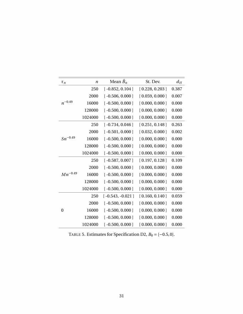
is B0 = [−1,0]. Specification D2 is similar, but with β0 =−0.3. In this case, the identified set is

B0 = [−0.5,0]. The objective functions are plotted in Figure 5 and the estimates are reported

in Tables 4 and 5. The estimator achieves arbitrarily fast convergence both cases, when the

slackness sequence is selected appropriately.

We proceed as before in constructing confidence sets, with the exception that we use the

scaling sequence bn = n1/2, so that the statistic Rn satisfies Assumption A6 (as established by

Theorem 9). The coverage frequencies are reported in Table 6. Because the population response

probabilities are exactly equal to one half for some values of x in Specification D1, the inference

procedure is non-degenerate. However, in Specification D2, while the inferential procedure is

valid, it is valid in a conservative sense.

6. Conclusion

This paper has developed asymptotic results for a class of criterion-function-based set estimators

which may exhibit non-standard behavior, such as cube-root consistency or arbitrarily fast

consistency. We have demonstrated these results by applying them to develop a robust set

estimator for semiparametric transformation models, and binary choice models in particular,

32

without the need to impose support conditions on the regressors. A series of Monte Carlo results

illustrates the theoretical results and provides insights into the practical finite sample behavior

of the estimator.

The general results established in this paper provide a basis for deriving the properties of

set estimators for other models and suggest several areas for future work in this literature. For

example, although we do not consider it explicitly here, the results could be generalized to

the closely-related multinomial choice model of Manski (1975) and other models based on

similar rank conditions. Finally, our Monte Carlo results suggest that further study of data-

driven procedures for selecting the constant of proportionality in the slackness sequence is an

interesting topic for future work.

A. Proofs

This section contains proofs for results not proven in the text. First we establish a preliminary

result regarding absolute values of functions, then we provide the remaining proofs in order.

Lemma 9. Let f and g be bounded real functions on A ⊂Rn . Then∣∣∣∣supx∈A

f (x)− supx∈A

g (x)

∣∣∣∣≤ supx∈A

∣∣ f (x)− g (x)∣∣ .

Proof of Lemma 9.

supx∈A

∣∣ f (x)− g (x)∣∣= sup

x∈A

[( f (x)− g (x))∨ (g (x)− f (x))

]= sup

x∈A[ f (x)− g (x)]∨ sup

x∈A[g (x)− f (x)]

≥ supx∈A

[f (x)− sup

y∈Ag (y)

]∨ sup

x∈A

[g (x)− sup

y∈Af (y)

]

=[

supx∈A

f (x)− supx∈A

g (x)

]∨

[supx∈A

g (x)− supx∈A

f (x)

]=

∣∣∣∣supx∈A

f (x)− supx∈A

g (x)

∣∣∣∣ .

■

Proof of Theorem 1. The proof proceeds in two steps. We first show that supθ∈Θnρ(θ,Θ1)

p→ 0.

Then, we show that limn→∞ P (Θ1 ⊂ Θn) = 1, which implies that supθ∈Θ1ρ(θ,Θn)

p→ 0. Combining

these steps and using the definition of the Hausdorff distance yields the final result.

33

Step 1 Let η> 0 and ε> 0 be given. Uniform convergence in probability of Qn to Q over the entire

parameter spaceΘ, from Assumption A3, also implies uniform convergence in probability over

the subset Θ \Θη1 , so we have both supΘ |Qn −Q| = Op (1/an) and supΘ\Θη1|Qn −Q| = Op (1/an).

Under Assumption A2, there exists a δη > 0 such that supΘ\Θη1

Q ≤ supΘQ −δη. Combining the

above results, we have

supΘ\Θ

η1

Qn ≤ supΘ\Θ

η1

Q +Op (1/an) ≤ supΘ

Q −δη+Op (1/an) ≤ supΘ

Qn −δη+Op (1/an).

Recall that by definition of Θn ,

infΘn

Qn ≥ supΘ

Qn −τn .

Since δη > 0 is constant and τn = op (1), there exists an integer nε such that for all n ≥ nε

with probability at least 1− ε both the Op (1/an) term and τn are smaller than δη/2 and so

−δη+Op (1/an) < −δη/2 < −τn . Therefore, for n ≥ nε, we have infΘnQn > supΘ\Θ

η1

Qn which

implies Θn ⊆ Θη1 which in turn implies supθ∈Θnρ(θ,Θ1) ≤ η, all with probability at least 1− ε.

Since ε and η were arbitrary, supθ∈Θnρ(θ,Θ1)

p→ 0.

Step 2 By definition of Θn , if supΘQn − infΘ1 Qn < τn , thenΘ1 ⊆ Θn . We have

supΘ

Qn − infΘ1

Qn =[

supΘ

Qn − supΘ

Q

]+

[supΘ

Q − infΘ1

Qn

]≤

∣∣∣∣supΘ

Qn − supΘ

Q

∣∣∣∣+ ∣∣∣∣supΘ

Q − infΘ1

Qn

∣∣∣∣=

∣∣∣∣supΘ

Qn − supΘ

Q

∣∣∣∣+ ∣∣∣∣infΘ1

Q − infΘ1

Qn

∣∣∣∣≤ sup

Θ|Qn −Q|+ sup

Θ1

|Qn −Q|

≤ 2supΘ

|Qn −Q| .

These steps follow by (1) adding and subtracting supΘQ, (2) taking the absolute value, (3) noting

thatΘ1 maximizes Q, (4) using the fact that inf f =−sup(− f ) and applying Lemma 9 twice, and

(5) recalling that Θ1 ⊆Θ. By Assumption A3, 2supΘ |Qn −Q| =Op (1/an). Finally, the condition

that τn approaches zero in probability slower than 1/an implies supΘQn − infΘ1 Qn < τn with

probability approaching one. ■

Proof of Theorem 2. Let ε> 0 be given and let δ, c, γ1, γ2, cε, and nε satisfy Assumption A4. Let

an satisfy Assumption A3 and define

νn ≡(

c1cε∨2τn an

anc1

)1/γ1

.

34

There exists an n′ε ≥ nε such that for all n ≥ n′

ε, with probability at least 1−ε each of the following

are true: (a) νn ≥ (cε/an)γ2 , (b) νn ≤ δ, and (c) supΘ |Qn −Q| ≤ τn . Condition (a) holds since

γ1γ2 ≥ 1 and so for sufficiently large n with probability at least 1−ε

ν1/γ2n ≥

(cεan

) 1γ1γ2 ≥ cε

an.

Condition (b) follows because νn = op (1), due to the assumptions on τn and an , and the fact

that δ is a strictly positive constant. Condition (c) follows from Assumption A3, under which

supΘ |Qn −Q| =Op (1/an), and the condition anτnp→∞. Therefore, for all n ≥ n′

ε, with probabil-

ity at least 1−ε,

supΘ\Θνn

1

Qn <(1)

supΘ

Q − c1(νn ∧δ)γ1 ≤(2)

supΘ

Q − c1νγ1n ≤

(3)supΘ

Q −2τn ≤(4)

supΘ

Qn −τn ≤(5)

infΘn

Qn .

Inequality (1) holds by Assumptions A2 and A4 and condition (a) under which ρ(θ,Θ1) > νn ≥(cε/an)γ2 for θ ∈ Θ \Θνn

1 . Inequality (2) is a direct result of condition (b). Inequality (3) holds

by definition of νn , since c1νγ1n ≥ 2τn . Inequality (4) follows from condition (c). Inequality (5)

follows by definition of Θn . It follows that for n ≥ n′ε, with probability at least 1− ε, the set

Θn ∩ (Θ \Θνn1 ) is empty, or equivalently, Θn ⊆ Θνn

1 . Finally, recall that by Theorem 1 we have

limn→∞ P (Θ1 ⊆ Θn) = 1. Therefore, for all n ≥ n′ε, with probability at least 1−ε, dH (Θn ,Θ1) ≤ νn

and hence dH (Θn ,Θ1) =Op (τγ2n ). ■

Proof of Theorem 3. First, note that that Assumption A4’ implies Assumption A2. Then, from The-

orem 1 we have limn→∞ P (Θ1 ⊆ Θn) = 1. We will prove the result by showing that limn→∞ P (Θn ⊆Θ1) = 1 and therefore the Hausdorff distance dH (Θn ,Θ1) equals zero with probability approach-

ing one. The logic is very similar to that used in Step 1 of the proof of Theorem 1, but without

expanding the setΘ1. We have

supΘ\Θ1

Qn ≤ supΘ\Θ1

Q +Op (1/an) ≤ supΘ

Q −δ+Op (1/an) ≤ supΘ

Qn −δ+Op (1/an),

where the first and last inequalities follow from Assumption A3 and the middle inequality

follows from Assumption A4’, the constant majorant condition. Since τn = op (1) and δ > 0 is

constant, with probability approaching one we have τn < δ/2 and Op (1/an) < δ/2, leading to

supΘ\Θ1Qn < supΘQn −τn ≤ infΘn

Qn , and therefore, Θn ⊆Θ1. ■

Proof of Theorem 4. The proof of Theorem 4 proceeds in three steps and follows the intuition

of Theorem 3.3 of Chernozhukov, Hong, and Tamer (2007). In our case, however, the limiting

distribution of Rn may not be continuous, in which case the confidence sets may be conservative

because the 1−α quantile of the distribution may be equal to higher quantiles as well. First,

we derive upper and lower bounds for Rn,m, j , defined in (5), such that Rn,m, j ≤ Rn,m, j ≤ Rn,m, j

35

with probability approaching one. Second, we prove that the distribution function of Rn,m, j

converges in probability to the distribution function of R (the limiting distribution of Rn), by

showing that the distribution functions of both of these bounds converge to that of R. Third, we

show that cn converges in probability to c(1−α), the desired quantile of the distribution of R.

Step 1 First, we restate the definition of Rn,m, j from (5):

Rn,m, j ≡ bm

(supθ∈Θ

Qn,m, j (θ)− infθ∈Θn

Qn,m, j (θ)

).

By Theorem 2, there exists a sequence εn ∝ τγ2n such that dH (Θn ,Θ1) ≤ εn and hence Θn ⊆Θεn

1

with probability approaching one. To establish the upper asymptotic bound, define Rn,m, j as

Rn,m, j but replace Θn byΘεn1 :

Rn,m, j ≡ bm

(supθ∈Θ

Qn,m, j (θ)− infθ∈Θεn

1

Qn,m, j (θ)

).

Then, for j = 1, . . . , Mn with probability approaching one we have infΘnQn,m, j ≥ infΘεn

1Qn,m, j ,

and therefore Rn,m, j ≤ Rn,m, j . To establish the lower bound, let Kn be the collection of all subsets

K ⊆Θ such that dH (K ,Θ1) ≤ εn and define Rn,m, j as Rn,m, j but replace Θn by the infimum over

all sets K ∈Kn :

Rn,m, j ≡ infK∈Kn

[bm

(supθ∈Θ

Qn,m, j (θ)− infθ∈K

Qn,m, j (θ)

)].

With probability approaching one, for each j there exists a set Θn,m, j ∈Kn such that Rn,m, j is

equal to the term in square brackets for K =Θn,m, j (in other words, Θn ∈ Kn). Therefore, for

j = 1, . . . , Mn with probability approaching one, Rn,m, j ≤ Rn,m, j .

Step 2 Let x be a continuity point of the distribution of R. From Step 1, with probability

approaching one,

Gn,m(x) ≡ 1

Mn

Mn∑j=1

1{Rn,m, j ≤ x} ≤ Gn,m(x) ≡ 1

Mn

Mn∑j=1

1{Rn,m, j ≤ x}

≤ Gn,m(x) ≡ 1

Mn

Mn∑j=1

1{Rn,m, j ≤ x}.

We will show that Gn,m(x)p→ P {R ≤ x}, Gn,m(x)

p→ P {R ≤ x}, and therefore Gn,m(x)p→ P {R ≤ x} as

n →∞ (and thus, as m →∞). Let J m denote the cdf of Rn,m, j . Note that Gn,m(x) is a U-statistic

of degree m. It is bounded since 0 ≤Gn,m(x) ≤ 1. Furthermore, E[Gn,m(x)] = E[1{Rn,m, j ≤ x}] =J m(x), where the last equality holds by nonreplacement sampling, since under Assumption A5

36

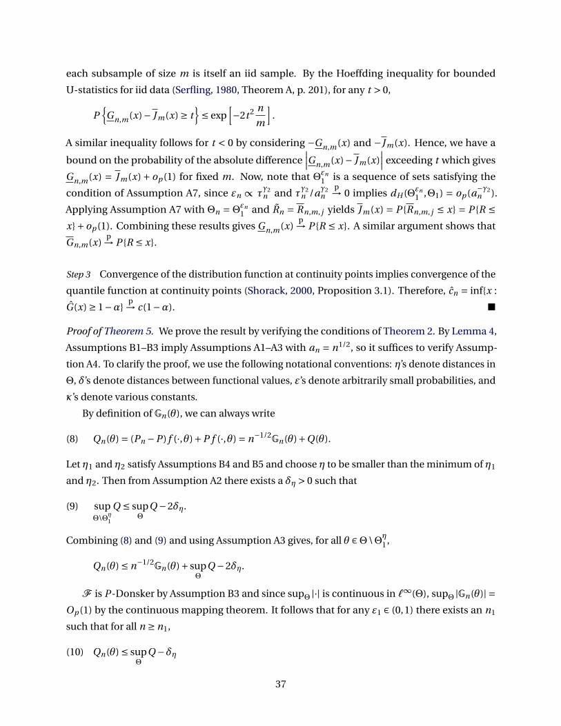
each subsample of size m is itself an iid sample. By the Hoeffding inequality for bounded

U-statistics for iid data (Serfling, 1980, Theorem A, p. 201), for any t > 0,

P{

Gn,m(x)− J m(x) ≥ t}≤ exp

[−2t 2 n

m

].

A similar inequality follows for t < 0 by considering −Gn,m(x) and −J m(x). Hence, we have a

bound on the probability of the absolute difference∣∣∣Gn,m(x)− J m(x)

∣∣∣ exceeding t which gives

Gn,m(x) = J m(x)+ op (1) for fixed m. Now, note that Θεn1 is a sequence of sets satisfying the

condition of Assumption A7, since εn ∝ τγ2n and τ

γ2n /aγ2

np→ 0 implies dH (Θεn

1 ,Θ1) = op (a−γ2n ).

Applying Assumption A7 with Θn = Θεn1 and Rn = Rn,m, j yields J m(x) = P {Rn,m, j ≤ x} = P {R ≤

x}+op (1). Combining these results gives Gn,m(x)p→ P {R ≤ x}. A similar argument shows that

Gn,m(x)p→ P {R ≤ x}.

Step 3 Convergence of the distribution function at continuity points implies convergence of the

quantile function at continuity points (Shorack, 2000, Proposition 3.1). Therefore, cn = inf{x :

G(x) ≥ 1−α}p→ c(1−α). ■

Proof of Theorem 5. We prove the result by verifying the conditions of Theorem 2. By Lemma 4,

Assumptions B1–B3 imply Assumptions A1–A3 with an = n1/2, so it suffices to verify Assump-

tion A4. To clarify the proof, we use the following notational conventions: η’s denote distances in

Θ, δ’s denote distances between functional values, ε’s denote arbitrarily small probabilities, and

κ’s denote various constants.

By definition of Gn(θ), we can always write

(8) Qn(θ) = (Pn −P ) f (·,θ)+P f (·,θ) = n−1/2Gn(θ)+Q(θ).

Let η1 and η2 satisfy Assumptions B4 and B5 and choose η to be smaller than the minimum of η1

and η2. Then from Assumption A2 there exists a δη > 0 such that

(9) supΘ\Θ

η1

Q ≤ supΘ

Q −2δη.

Combining (8) and (9) and using Assumption A3 gives, for all θ ∈Θ\Θη1 ,

Qn(θ) ≤ n−1/2Gn(θ)+ supΘ

Q −2δη.

F is P-Donsker by Assumption B3 and since supΘ |·| is continuous in `∞(Θ), supΘ |Gn(θ)| =Op (1) by the continuous mapping theorem. It follows that for any ε1 ∈ (0,1) there exists an n1

such that for all n ≥ n1,

(10) Qn(θ) ≤ supΘ

Q −δη

37

uniformly onΘ\Θη1 with probability at least 1−ε1.

Now, by Assumption B4, there is a neighborhood Θη11 of Θ1 such that Q is approximately

quadratic in the directed distance ρ(θ,Θ1). That is, for some κ1 > 0,

Q(θ) ≤ supΘ

Q −κ1ρ2(θ,Θ1)

for all θ ∈Θη11 . Similarly, by Assumption B5 and Lemma 4.1 of Kim and Pollard (1990), for all

κ2 > 0 there exists a sequence of random variables Mn =Op (1) such that

(11)∣∣(Pn −P ) f (·,θ)

∣∣≤ κ2ρ2(θ,Θ1)+n−2/3M 2

n

for θ ∈Θη21 . Combining these results for κ2 = κ1/2 and using (8) and Assumption A3 yields

Qn(θ) ≤ supΘ

Q − κ1

2ρ2(θ,Θ1)+n−2/3M 2

n

for all θ ∈Θη1∧η21 .

Notice that when n−2/3M 2n is smaller than (κ1/4)ρ2(θ,Θ1), we have

(12) Qn(θ) ≤ supΘ

Q − κ1

4ρ2(θ,Θ1),

which is a polynomial majorant of the form required by Assumption A4. This is true whenever

ρ(θ,Θ1) ≥ 4κ−1/21 n−1/3Mn . Since Mn = Op (1), for any ε3 ∈ (0,1), there exists a κ3 and n3 such

that for all n ≥ n3, ρ(θ,Θ1) ≥ κ3n−1/3 ≥ 4κ−1/21 n−1/3Mn and the bound in (12) holds uniformly on

Θη1 \Θκ3n−1/3

1 with probability at least 1−ε3. (Note that we can always choose n3 large enough

so that κ3n−1/3 is smaller than η < η1 ∧η2, ensuring that the relevant region of the domain is

nonempty.)

To show that Assumption A4 holds, let ε ∈ (0,1) be given. For ε1 = ε/2, choose n1 and δη as

above so that (10) holds uniformly onΘ\Θη1 with probability at least 1−ε1. Then, for ε3 = ε/2,

choose n3 and κ3 such that (12) holds uniformly onΘη1 \Θκ3n−1/3

1 with probability at least 1−ε3.

To summarize, we have shown that

Qn(θ) ≤ supΘ

Q −max{κ1

4ρ2(θ,Θ1),δη

}uniformly onΘ\Θκ3n−1/3

1 with probability at least 1−ε. It follows that Assumption A4 holds with

an = n1/2, δ = δη, c = κ1/4, γ1 = 2, γ2 = 2/3, cε = κ3, and nε = max{n1,n3}. Therefore, for any

sequence rn such that rn = o(n1/3), let τn ∝ r−3/2n . Since n1/3r−1

n →∞, we have (n1/3r−1n )3/2 =

n1/2r−3/2n ∝ n1/2τn

p→∞ and therefore Theorem 2 implies dH (Θn ,Θ1) =Op (τ2/3n ) =Op (r−1

n ). ■

38

Proof of Theorem 6. We verify the sufficient conditions for consistency of Lemma 4, with an =n1/2. Assumptions B1 and B2 were verified above, therefore it only remains to show that F is

manageable for an envelope F for which PF 2 <∞.

Let α,γ ∈R and δ ∈Rk . For each (x, y, t ) ∈X ×{0,1}×R, define g (x, y, t ;α,γ,δ) =αt +γy +δ′xand G = {g (·, ·, ·;α,γ,δ) : α,γ ∈ R and δ ∈ Rk }. Since G is a finite-dimensional vector space of

real-valued functions on X × {0,1}×R, classes of sets of the form {g ≥ r } or {g > r } with g ∈ G

and r ∈ R are VC classes (Pakes and Pollard, 1989, Lemma 2.4). We will use particular choices

of α, γ, and δ to show that F is VC subgraph class, that is, that the collection of subgraphs of

functions in F is a VC class.

First, note that we can rewrite f as

f (x, y,θ) = (1{y > 0}−1{y ≤ 0}

)(1{x ′θ ≥ 0}−1{x ′θ < 0}

)= 1{y > 0, x ′θ ≥ 0}−1{y > 0, x ′θ < 0}−1{y ≤ 0, x ′θ ≥ 0}+1{y ≤ 0, x ′θ < 0}.

For any θ ∈Θ,

subgraph(

f (·, ·,θ))= {

(x, y, t ) ∈X × {0,1}×R : 0 < t < f (x, y,θ) or 0 > t > f (x, y,θ)}

= ({y > 0}∩ {x ′θ ≥ 0}∩ {t ≥ 1}c ∩ {t > 0}

)∪ (

{y > 0}∩ {x ′θ ≥ 0}c ∩ {t >−1}∩ {t ≥ 0}c)∪ (

{y ≥ 0}c ∩ {x ′θ ≥ 0}∩ {t >−1}∩ {t ≥ 0}c)∪ (

{y ≥ 0}c ∩ {x ′θ < 0}∩ {t ≥ 1}c ∩ {t > 0})

.

Now, we construct three functions of the form g j (x, y, t ) =α j t+γ j z+δ′j x with g j ∈G for j = 1,2,3

by choosing coefficients α1 = 0, γ1 = 1, δ1 = 0, α2 = 0, γ2 = 0, δ2 = θ, α3 = 1, γ3 = 0, and δ3 = 0.

Then

subgraph(

f (·, ·,θ))= (

{g1 > 0}∩ {g2 ≥ 0}∩ {g3 ≥ 1}c ∩ {g3 > 0})

∪ ({g1 > 0}∩ {g2 ≥ 0}c ∩ {g3 >−1}∩ {g3 ≥ 0}c)

∪ ({g1 ≥ 0}c ∩ {g2 ≥ 0}∩ {g3 >−1}∩ {g3 ≥ 0}c)

∪ ({g1 ≥ 0}c ∩ {g2 < 0}∩ {g3 ≥ 1}c ∩ {g3 > 0}

).

Since sets of the form {g ≥ 0} or {g > 0} for g ∈ G are VC classes and since this property is

preserved over complements, unions, and intersections (Pakes and Pollard, 1989, Lemma 2.5), it

follows that {subgraph( f ) : f ∈F } is itself a VC class. By Lemma 2.12 of Pakes and Pollard (1989),

F is Euclidean for every envelope, including constant envelope F = 1. Since it is Euclidean, F is

also manageable in the sense of Pollard (1989) (cf. Pakes and Pollard, 1989, p. 1033) as required

by Assumption B3. ■

39

Proof of Theorem 7. Following Abrevaya and Huang (2005), we work with the re-normalized

objective function based on f (x, y,β) = (2y −1)(1{x ′β+xk ≥ 0}−1{x ′β+xk ≥ 0}) for some β ∈ B0,

which is equivalent to adding a constant to the objective function. We prove the result by verifying

Assumptions B1–B5 and using Theorem 5. Assumptions B1–B3 have been verified already by

Theorem 6.

Under assumptions a–f, it follows from Abrevaya and Huang (2005, p. 1200) that ∇ββ′ Q(β) =−V (β) for all β ∈ bd(B0) (where V (β) is defined in assumption f). Therefore, in a neighborhood

N of B0, Q is approximately quadratic and for some c > 0, Q(β) ≤ supQ−cρ2(β,B0). This verifies

Assumption B4.

To show that Assumption B5 holds, let η> 0 and define Fη ≡ { f (·,β) ∈F : ρ(β,B0) ≤ η}. We

will show that the natural envelope Fη of Fη is such that PF 2η =O(η). First, note that by definition

of Fη if f (·,β) ∈Fη, then β ∈ Bη0 . Then,

Fη(x, y) = supβ∈B

η0

∣∣ f (x, y,β)∣∣

= supβ∈B

η0

∣∣1{x ′β≥−xk > x ′β}+1{x ′β≥−xk > x ′β}∣∣

≤ supβ∈B

η0

1{−‖x‖ ·∥∥β− β∥∥≤ x ′β+xk ≤ ‖x‖ ·∥∥β− β∥∥}

.

Now, for all β ∈ Bη0 and β ∈ B0, we have∥∥β− β∥∥≤ ρ(β,bd(B0))+dH (bd(B0), int(B0)) ≤ η+δ

where δ≡ dH (bd(B0), int(B0)) is the largest distance from some point on the interior of B0 to the

boundary of B0. Therefore Fη(x, y) ≤ 1{−(η+δ)‖x‖ ≤ x ′β+xk ≤ (η+δ)‖x‖} and

PF 2η ≤

∫X

∫{

xk∈Xk :−(η+δ)‖x‖≤x ′β+xk≤(η+δ)‖x‖} dFxk |x(xk | x)dFx(x)

≤ 2(η+δ)∫X

supxk∈Xk

fxk |x(xk | x) · ‖x‖ dFx(x).

Since x has finite first absolute moments (assumption a), fxk |x(xk | x) is finite for almost every

x (assumption b), and δ < ∞ since B0 is compact (assumption e), this bound is finite and

PF 2η =O(η). ■

Proof of Theorem 9. Assumption A7 holds in both cases (a) and (b) due to uniform convergence

in probability, which implies stochastic equicontinuity. It remains to verify Assumption A6.

Case (a) Suppose that Assumption C2 holds and bn = n1/2. Since supΘQ is a constant and

Q(θ) = supΘQ for all θ ∈Θ1, we can restate Rn as

Rn = n1/2[

supΘ

Qn − infΘ1

Qn

]= n1/2

[(supΘ

Qn − supΘ

Q

)− infΘ1

(Qn −Q)

].

40

Then,

|Rn | ≤ supΘ

∣∣n1/2(Qn −Q)∣∣+ inf

Θ1

∣∣n1/2(Qn −Q)∣∣= sup

Θ|Gn |+ inf

Θ1|Gn | =Op (1),

where the final equality follows because F is P-Donsker.

Case (b) Suppose that Assumption C1 holds and bn = n2/3. For the following, we rely on two

intermediate results from the proof of Theorem 5 above. First, let η satisfy Assumption B5 and

note that from (11), for all c > 0 there exists a sequence of random variables Mn = Op (1) such

that

Qn(θ) ≤Q(θ)+ cρ2(θ,Θ1)+n−2/3M 2n

for all θ ∈ Θη1 . Second, from (12) there exists a κ > 0 such that Qn is maximized on Θκn−1/3

1

with probability approaching one. Then, with probability approaching one we have supΘQn =sup

Θκn−1/31

Qn and Θκn−1/3

1 ⊂ Θη1 . Also note that supΘ1Q = infΘ1 Q = supΘQ by definition of Θ1.

Combining these results, with probability approaching one we have

0 ≤ Rn = n2/3

supΘκn−1/3

1

Qn − infΘ1

Qn

≤ c ·n2/3

supΘκn−1/3

1

ρ2(θ,Θ1)− infΘ1ρ2(θ,Θ1)

= cκ2 <∞

since supΘκn−1/3

1ρ2(θ,Θ1) = κ2n−2/3 and infΘ1 ρ

2(θ,Θ1) = 0. Therefore, Rn =Op (1) as asserted. ■

References

Abrevaya, J. (2000). Rank estimation of a generalized fixed-effects regression model. Journal of

Econometrics 95, 1–23.

Abrevaya, J. and J. Huang (2005). On the bootstrap of the maximum score estimator. Economet-

rica 73, 1175–1204.

Amemiya, T. (1985). Advanced Econometrics. Harvard University Press.

Andrews, D. and P. Guggenberger (2008). Asymptotics for stationary very nearly unit root

processes. Journal of Time Series Analysis 29, 203–212.

Andrews, D. W. K., S. Berry, and P. Jia (2004). Confidence regions for parameters in discrete games

with multiple equilibria, with an application to discount chain store location. Working paper,

Yale University.

41

Andrews, D. W. K. and P. Guggenberger (2009). Validity of subsampling and “plug-in asymptotic”

inference for parameters defined by moment inequalities. Econometric Theory 25, 669–709.

Andrews, D. W. K. and X. Shi (2013). Inference based on conditional moment inequalities.

Econometrica 81, 609–666.

Andrews, D. W. K. and G. Soares (2010). Inference for parameters defined by moment inequalities

using generalized moment selection. Econometrica 78, 119–158.

Bajari, P., J. T. Fox, and S. P. Ryan (2008). Evaluating wireless carrier consolidation using semi-

parametric demand estimation. Quantitative Marketing and Economics 6, 299–338.

Beresteanu, A., I. Molchanov, and F. Molinari (2011). Sharp identification regions in models with

convex moment predictions. Econometrica 79, 1785–1821.

Beresteanu, A. and F. Molinari (2008). Asymptotic properties for a class of partially identified

models. Econometrica 76, 763–814.

Bhattacharya, D. (2009). Inferring optimal peer assignment from experimental data. Journal of

the American Statistical Association 104, 486–500.

Bierens, H. J. and J. Hartog (1988). Non-linear regression with discrete explanatory variables,

with an application to the earnings function. Journal of Econometrics 38, 269–299.

Bugni, F. A. (2010). Bootstrap inference in partially identified models defined by moment

inequalities: Coverage of the identified set. Econometrica 78, 735–753.

Canay, I. A. (2010). EL inference for partially identified models: Large deviations optimality and

bootstrap validity. Journal of Econometrics 156, 408–425.

Chernozhukov, V., H. Hong, and E. Tamer (2007). Estimation and confidence regions for parame-

ter sets in econometric models. Econometrica 75, 1243–1284.

Cosslett, S. R. (1983). Distribution-free maximum likelihood estimation of the binary choice

model. Econometrica 51, 765–782.

Dudley, R. M. (1987). Universal Donsker classes and metric entropy. Annals of Probability 15,

1306–1326.

Han, A. K. (1987). Non-parametric analysis of a generalized regression model: The maximum

rank correlation estimator. Journal of Econometrics 35, 303–316.

42

Honoré, B. E. and A. Lleras-Muney (2006). Bounds in competing risks models and the war on

cancer. Econometrica 74, 1675–1698.

Honoré, B. E. and E. Tamer (2006). Bounds on parameters in panel dynamic discrete choice

models. Econometrica 74, 611–629.

Horowitz, J. L. (1992). A smoothed maximum score estimator for the binary response model.

Econometrica 60, 505–531.

Horowitz, J. L. (1998). Semiparametric Methods in Econometrics. New York: Springer.

Ichimura, H. (1993). Semiparametric least squares (SLS) and weighted SLS estimation of single-

index models. Journal of Econometrics 58, 71–120.

Imbens, G. W. and C. F. Manski (2004). Confidence intervals for partially identified parameters.

Econometrica 72, 1845–1857.

Jun, S., J. Pinkse, and Y. Wan (2011). Classical Laplace estimation for 3p

n-consistent estimators:

Improved convergence rates and rate-adaptive inference. Working paper, Pennsylvania State

University.

Khan, S. and E. Tamer (2009). Inference on endogenously censored regression models using

conditional moment inequalities. Journal of Econometrics 152, 104–119.

Kim, J. and D. Pollard (1990). Cube root asymptotics. The Annals of Statistics 18, 191–219.

Kim, K. (2008). Set estimation and inference with models characterized by conditional moment

inequalities. Working paper, University of Minnesota.

Klein, R. W. and R. H. Spady (1993). An efficient semiparametric estimator for binary response

models. Econometrica 61, 387–421.

Komarova, T. (2008). Binary choice models with discrete regressors: Identification and misspeci-

fication. Working paper, London School of Economics.

Lewbel, A. (2000). Semiparametric qualitative response model estimation with unknown het-

eroskedasticity or instrumental variables. Journal of Econometrics 97, 145–177.

Maddala, G. S. (1983). Limited-Dependent and Qualitative Variables in Econometrics. Cambridge

University Press.

Magnac, T. and E. Maurin (2008). Partial identification in monotone binary models: Discrete

regressors and interval data. Review of Economic Studies 75, 835–864.

43

Manski, C. F. (1975). Maximum score estimation of the stochastic utility model of choice. Journal

of Econometrics 3, 205–228.

Manski, C. F. (1985). Semiparametric analysis of discrete response: Asymptotic properties of the

maximum score estimator. Journal of Econometrics 27, 313–333.

Manski, C. F. (1987). Semiparametric analysis of random effects linear models from binary panel

data. Econometrica 55, 357–362.

Manski, C. F. (1988). Identification of binary response models. Journal of the American Statistical

Association 83, 729–738.

Manski, C. F. (2003). Partial Identification of Probability Distributions. Springer-Verlag.

Manski, C. F. and E. Tamer (2002). Inference on regressions with interval data on a regressor or

outcome. Econometrica 70, 519–546.

Matzkin, R. L. (1992). Nonparametric and distribution-free estimation of the binary threshold

crossing and the binary choice models. Econometrica 60, 239–270.

McFadden, D. L. (1974). Conditional logit analysis of qualitative choice analysis. In P. Zarembka

(Ed.), Frontiers in Econometrics, pp. 105–142. Academic Press.

Menzel, K. (2008). Estimation and inference with many moment inequalities. Working paper,

Massachussetts Institute of Technology.

Newey, W. K. and D. McFadden (1994). Large sample estimation and hypothesis testing. In

R. F. Engle and D. McFadden (Eds.), Handbook of Econometrics, Volume 4, Amsterdam. New

Holland.

Nolan, D. and D. Pollard (1987). U -Processes: Rates of convergence. Annals of Statistics 15,

780–799.

Pakes, A. and D. Pollard (1989). Simulation and the asymptotics of optimization estimators.

Econometrica 57, 1027–1057.

Pakes, A., J. Porter, K. Ho, and J. Ishii (2006). Moment inequalities and their application. Working

paper, Harvard University.

Politis, D. N., J. P. Romano, and M. Wolf (1999). Subsampling. Springer.

Pollard, D. (1989). Asymptotics via empirical processes. Statistical Science 4, 341–366.

44

Romano, J. P. and A. M. Shaikh (2008). Inference for identifiable parameters in partially identified

econometric models. Journal of Statistical Planning and Inference 138, 2786–2807.

Romano, J. P. and A. M. Shaikh (2010). Inference for the identified set in partially identified

econometric models. Econometrica 78, 169–211.

Serfling, R. J. (1980). Approximation Theorems of Mathematical Statistics. Wiley.

Shorack, G. R. (2000). Probability for Statisticians. Springer.

Stoker, T. M. (1986). Consistent estimation of scaled coefficients. Econometrica 54, 1461–1481.

Stoye, J. (2009). More on confidence intervals for partially identified parameters. Econometrica 77,

1299–1315.

Tamer, E. (2010). Partial identification in econometrics. Annual Review of Economics 2, 167–195.

van der Vaart, A. W. (1998). Asymptotic Statistics. Cambridge University Press.

Yildiz, N. (2012). Consistency of plug-in estimators of upper contour and level sets. Econometric

Theory 28, 309–327.

45