non-quadratic regularization of the inverse problem...
TRANSCRIPT

Non-quadratic Regularization of the Inverse ProblemAssociated to the Black-Scholes PDE
UNDER CAPRICORN 1
Thanks to Antonio Leitao!!!
V. Albani (IMPA)A. De Cezaro (FURG,Brazil)
O. Scherzer (U.Vienna, Austria)Jorge P. Zubelli
IMPA
September 2, 2011
1credit to Alvaro De PierroRegularization of Local Vol c©J.P.Zubelli (IMPA)
September 2, 2011 1 /55

Outline
1 Intro
2 Motivation and Goals
3 Background
4 Problem Statement and Results on Local Vol Models
5 Main Technical Results
6 Numerical Examples
7 Conclusions
Regularization of Local Vol c©J.P.Zubelli (IMPA)September 2, 2011 2 /
55

Options, Derivatives, Futures
Why?
HEDGING Risk Reduction/Protection
When? Anytime there is uncertainty
Who? LOTS OF PEOPLE! (Derivative markets are bigger than theunderlying ones!)Examples
Fixed Income (otc, bonds, etc)Insurance MarketsPension FundsCurrency Markets
Remark: Good estimation of the local volatility is crucial for the consistentpricing of other contracts (in particular exotic derivatives).
Regularization of Local Vol c©J.P.Zubelli (IMPA)September 2, 2011 3 /
55

Options, Derivatives, Futures
Why? HEDGING
Risk Reduction/Protection
When? Anytime there is uncertainty
Who? LOTS OF PEOPLE! (Derivative markets are bigger than theunderlying ones!)Examples
Fixed Income (otc, bonds, etc)Insurance MarketsPension FundsCurrency Markets
Remark: Good estimation of the local volatility is crucial for the consistentpricing of other contracts (in particular exotic derivatives).
Regularization of Local Vol c©J.P.Zubelli (IMPA)September 2, 2011 3 /
55
Options, Derivatives, Futures
Why? HEDGING Risk Reduction/Protection
When? Anytime there is uncertainty
Who? LOTS OF PEOPLE! (Derivative markets are bigger than theunderlying ones!)Examples
Fixed Income (otc, bonds, etc)Insurance MarketsPension FundsCurrency Markets
Remark: Good estimation of the local volatility is crucial for the consistentpricing of other contracts (in particular exotic derivatives).
Regularization of Local Vol c©J.P.Zubelli (IMPA)September 2, 2011 3 /
55

Options, Derivatives, Futures
Why? HEDGING Risk Reduction/Protection
When?
Anytime there is uncertainty
Who? LOTS OF PEOPLE! (Derivative markets are bigger than theunderlying ones!)Examples
Fixed Income (otc, bonds, etc)Insurance MarketsPension FundsCurrency Markets
Remark: Good estimation of the local volatility is crucial for the consistentpricing of other contracts (in particular exotic derivatives).
Regularization of Local Vol c©J.P.Zubelli (IMPA)September 2, 2011 3 /
55
Options, Derivatives, Futures
Why? HEDGING Risk Reduction/Protection
When? Anytime there is uncertainty
Who? LOTS OF PEOPLE! (Derivative markets are bigger than theunderlying ones!)Examples
Fixed Income (otc, bonds, etc)Insurance MarketsPension FundsCurrency Markets
Remark: Good estimation of the local volatility is crucial for the consistentpricing of other contracts (in particular exotic derivatives).
Regularization of Local Vol c©J.P.Zubelli (IMPA)September 2, 2011 3 /
55

Options, Derivatives, Futures
Why? HEDGING Risk Reduction/Protection
When? Anytime there is uncertainty
Who?
LOTS OF PEOPLE! (Derivative markets are bigger than theunderlying ones!)Examples
Fixed Income (otc, bonds, etc)Insurance MarketsPension FundsCurrency Markets
Remark: Good estimation of the local volatility is crucial for the consistentpricing of other contracts (in particular exotic derivatives).
Regularization of Local Vol c©J.P.Zubelli (IMPA)September 2, 2011 3 /
55

Options, Derivatives, Futures
Why? HEDGING Risk Reduction/Protection
When? Anytime there is uncertainty
Who? LOTS OF PEOPLE! (Derivative markets are bigger than theunderlying ones!)Examples
Fixed Income (otc, bonds, etc)Insurance MarketsPension FundsCurrency Markets
Remark: Good estimation of the local volatility is crucial for the consistentpricing of other contracts (in particular exotic derivatives).
Regularization of Local Vol c©J.P.Zubelli (IMPA)September 2, 2011 3 /
55

Options, Derivatives, Futures
Why? HEDGING Risk Reduction/Protection
When? Anytime there is uncertainty
Who? LOTS OF PEOPLE! (Derivative markets are bigger than theunderlying ones!)Examples
Fixed Income (otc, bonds, etc)Insurance MarketsPension FundsCurrency Markets
Remark: Good estimation of the local volatility is crucial for the consistentpricing of other contracts (in particular exotic derivatives).
Regularization of Local Vol c©J.P.Zubelli (IMPA)September 2, 2011 3 /
55

Derivative Contracts
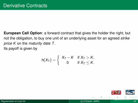
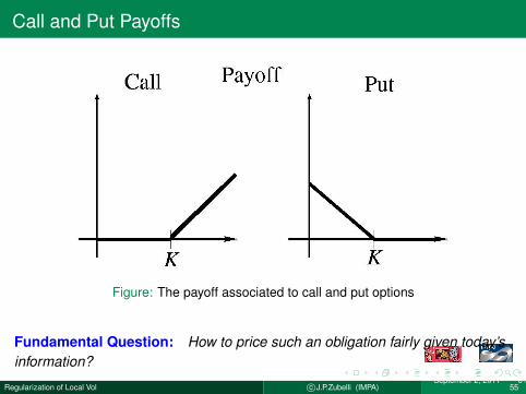
European Call Option: a forward contract that gives the holder the right, butnot the obligation, to buy one unit of an underlying asset for an agreed strikeprice K on the maturity date T .
Its payoff is given by
h(XT ) =
XT −K if XT > K ,
0 if XT ≤ K .
Regularization of Local Vol c©J.P.Zubelli (IMPA)September 2, 2011 4 /
55
Derivative Contracts
European Call Option: a forward contract that gives the holder the right, butnot the obligation, to buy one unit of an underlying asset for an agreed strikeprice K on the maturity date T .Its payoff is given by
h(XT ) =
XT −K if XT > K ,
0 if XT ≤ K .
Regularization of Local Vol c©J.P.Zubelli (IMPA)September 2, 2011 4 /
55
Derivative Contracts
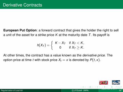
European Put Option: a forward contract that gives the holder the right to sella unit of the asset for a strike price K at the maturity date T . Its payoff is
h(XT ) =
K −XT if XT < K ,
0 if XT ≥ K .
At other times, the contract has a value known as the derivative price. Theoption price at time t with stock price Xt = x is denoted by P(t,x).
Regularization of Local Vol c©J.P.Zubelli (IMPA)September 2, 2011 5 /
55
Call and Put Payoffs
Figure: The payoff associated to call and put options
Fundamental Question: How to price such an obligation fairly given today’sinformation?
Regularization of Local Vol c©J.P.Zubelli (IMPA)September 2, 2011 6 /
55

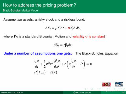
How to address the pricing problem?Black-Scholes Market Model
Assume two assets: a risky stock and a riskless bond.
dXt = µXtdt + σXtdWt ,
where Wt is a standard Brownian Motion and volatility σ is constant
dβt = rβtdt.
Under a number of assumptions one gets: The Black-Scholes Equation
∂P∂t
+12
σ2x2 ∂2P
∂x2 + r
(x
∂P∂x−P
)= 0
P(T ,x) = h(x)
Note 1: P = P(t,x ;σ, r) for t ≤ T .Note 2: Final Value Problem
Regularization of Local Vol c©J.P.Zubelli (IMPA)September 2, 2011 7 /
55

How to address the pricing problem?Black-Scholes Market Model
Assume two assets: a risky stock and a riskless bond.
dXt = µXtdt + σXtdWt ,
where Wt is a standard Brownian Motion and volatility σ is constant
dβt = rβtdt.
Under a number of assumptions one gets: The Black-Scholes Equation
∂P∂t
+12
σ2x2 ∂2P
∂x2 + r
(x
∂P∂x−P
)= 0
P(T ,x) = h(x)
Note 1: P = P(t,x ;σ, r) for t ≤ T .
Note 2: Final Value Problem
Regularization of Local Vol c©J.P.Zubelli (IMPA)September 2, 2011 7 /
55

How to address the pricing problem?Black-Scholes Market Model
Assume two assets: a risky stock and a riskless bond.
dXt = µXtdt + σXtdWt ,
where Wt is a standard Brownian Motion and volatility σ is constant
dβt = rβtdt.
Under a number of assumptions one gets: The Black-Scholes Equation
∂P∂t
+12
σ2x2 ∂2P
∂x2 + r
(x
∂P∂x−P
)= 0
P(T ,x) = h(x)
Note 1: P = P(t,x ;σ, r) for t ≤ T .Note 2: Final Value Problem
Regularization of Local Vol c©J.P.Zubelli (IMPA)September 2, 2011 7 /
55

Main Contributions
Figure: L. Bachelier
L. Bachelier (Paris)
P. Samuelson
F. Black
M. Scholes
R. Merton
Regularization of Local Vol c©J.P.Zubelli (IMPA)September 2, 2011 8 /
55
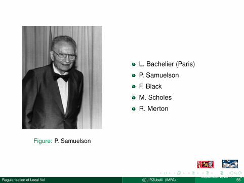
Figure: P. Samuelson
L. Bachelier (Paris)
P. Samuelson
F. Black
M. Scholes
R. Merton
Regularization of Local Vol c©J.P.Zubelli (IMPA)September 2, 2011 9 /
55
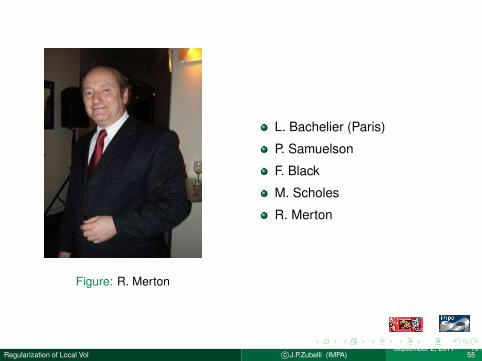
Figure: R. Merton
L. Bachelier (Paris)
P. Samuelson
F. Black
M. Scholes
R. Merton
Regularization of Local Vol c©J.P.Zubelli (IMPA)September 2, 2011 10 /
55
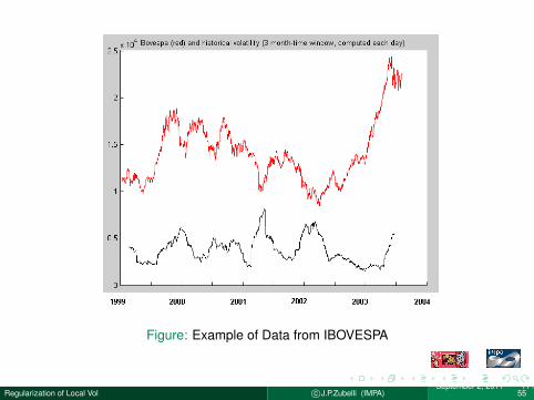
Figure: Example of Data from IBOVESPA
Regularization of Local Vol c©J.P.Zubelli (IMPA)September 2, 2011 11 /
55

Figure: Example of the Solution to Black-Scholes
Regularization of Local Vol c©J.P.Zubelli (IMPA)September 2, 2011 12 /
55

Motivation and Goals
Good model selection is crucial for modern sound financial practice.
Focus: Dupire [Dup94] local volatility modelsGoal:
Present a unified framework for the calibration of local volatility models
Use recent tools of convex regularization of ill-posed Inverse Problems.
Present convergence results that include convergence rates w.r.t. noiselevel in fairly general contexts
Go beyond the classical quadratic regularization.
ApplicationVolatility surface calibration is crucial in many applications. E.G.: riskmanagement, hedging, and the evaluation of exotic derivatives.
Regularization of Local Vol c©J.P.Zubelli (IMPA)September 2, 2011 13 /
55
Motivation and Goals
Good model selection is crucial for modern sound financial practice.Focus: Dupire [Dup94] local volatility models
Goal:
Present a unified framework for the calibration of local volatility models
Use recent tools of convex regularization of ill-posed Inverse Problems.
Present convergence results that include convergence rates w.r.t. noiselevel in fairly general contexts
Go beyond the classical quadratic regularization.
ApplicationVolatility surface calibration is crucial in many applications. E.G.: riskmanagement, hedging, and the evaluation of exotic derivatives.
Regularization of Local Vol c©J.P.Zubelli (IMPA)September 2, 2011 13 /
55

Motivation and Goals
Good model selection is crucial for modern sound financial practice.Focus: Dupire [Dup94] local volatility modelsGoal:
Present a unified framework for the calibration of local volatility models
Use recent tools of convex regularization of ill-posed Inverse Problems.
Present convergence results that include convergence rates w.r.t. noiselevel in fairly general contexts
Go beyond the classical quadratic regularization.
ApplicationVolatility surface calibration is crucial in many applications. E.G.: riskmanagement, hedging, and the evaluation of exotic derivatives.
Regularization of Local Vol c©J.P.Zubelli (IMPA)September 2, 2011 13 /
55
Main Features
Address in a general and rigorous way the key issue of convergence andsensitivity of the regularized solution when the noise level of the observedprices goes to zero.
Our approach relates to different techniques in volatility surfaceestimation. e.g.: the Statistical concept of exponential families andentropy-based estimation.
Our framework connects with the Financial concept of Convex RiskMeasures.
Regularization of Local Vol c©J.P.Zubelli (IMPA)September 2, 2011 14 /
55

Limitations of Classical Black-Scholes
log-normality of asset prices is not verified by statistical tests
option prices are subjet to the smile effects
volatility of the prices tends fluctuate with time and revert to a mean value
Regularization of Local Vol c©J.P.Zubelli (IMPA)September 2, 2011 15 /
55
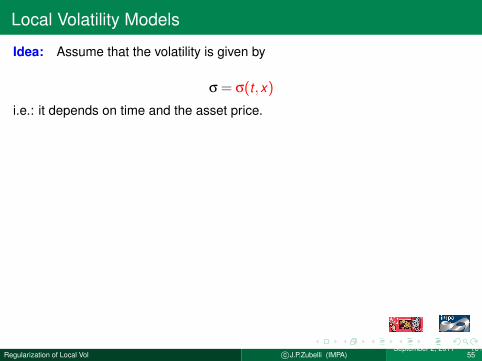
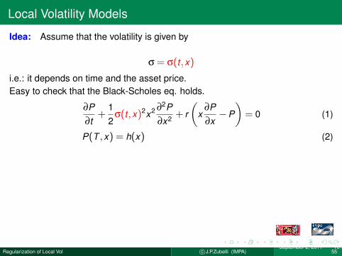
Local Volatility Models
Idea: Assume that the volatility is given by
σ = σ(t,x)
i.e.: it depends on time and the asset price.
Easy to check that the Black-Scholes eq. holds.
∂P∂t
+12
σ(t,x)2x2 ∂2P∂x2 + r
(x
∂P∂x−P
)= 0 (1)
P(T ,x) = h(x) (2)
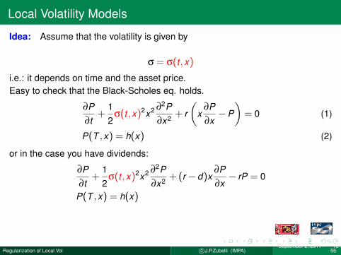
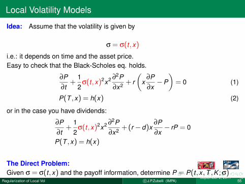
or in the case you have dividends:
∂P∂t
+12
σ(t,x)2x2 ∂2P∂x2 + (r −d)x
∂P∂x− rP = 0
P(T ,x) = h(x)
The Direct Problem:Given σ = σ(t,x) and the payoff information, determine P = P(t,x ,T ,K ;σ)
Regularization of Local Vol c©J.P.Zubelli (IMPA)September 2, 2011 16 /
55
Local Volatility Models
Idea: Assume that the volatility is given by
σ = σ(t,x)
i.e.: it depends on time and the asset price.Easy to check that the Black-Scholes eq. holds.
∂P∂t
+12
σ(t,x)2x2 ∂2P∂x2 + r
(x
∂P∂x−P
)= 0 (1)
P(T ,x) = h(x) (2)
or in the case you have dividends:
∂P∂t
+12
σ(t,x)2x2 ∂2P∂x2 + (r −d)x
∂P∂x− rP = 0
P(T ,x) = h(x)
The Direct Problem:Given σ = σ(t,x) and the payoff information, determine P = P(t,x ,T ,K ;σ)
Regularization of Local Vol c©J.P.Zubelli (IMPA)September 2, 2011 16 /
55
The Inverse Problem
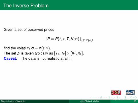
Given a set of observed prices
P = P(t,x ,T ,K ;σ)(T ,K )∈S
find the volatility σ = σ(t,x).The set S is taken typically as [T1,T2]× [K1,K2].Caveat: The data is not realistic at all!!!
In Practice: Very limited and scarce dataNote: To price in a consistent way the so-called exotic derivatives one has toknow σ and not only the transition probabilities
Regularization of Local Vol c©J.P.Zubelli (IMPA)September 2, 2011 17 /
55

The Inverse Problem
Given a set of observed prices
P = P(t,x ,T ,K ;σ)(T ,K )∈S
find the volatility σ = σ(t,x).The set S is taken typically as [T1,T2]× [K1,K2].Caveat: The data is not realistic at all!!!In Practice: Very limited and scarce data
Note: To price in a consistent way the so-called exotic derivatives one has toknow σ and not only the transition probabilities
Regularization of Local Vol c©J.P.Zubelli (IMPA)September 2, 2011 17 /
55

The Inverse Problem
Given a set of observed prices
P = P(t,x ,T ,K ;σ)(T ,K )∈S
find the volatility σ = σ(t,x).The set S is taken typically as [T1,T2]× [K1,K2].Caveat: The data is not realistic at all!!!In Practice: Very limited and scarce dataNote: To price in a consistent way the so-called exotic derivatives one has toknow σ and not only the transition probabilities
Regularization of Local Vol c©J.P.Zubelli (IMPA)September 2, 2011 17 /
55
The Smile Curve and Dupire’s Equation
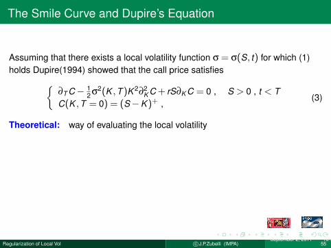
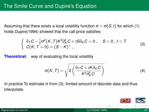
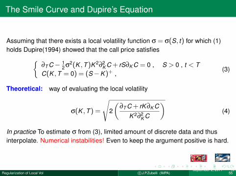
Assuming that there exists a local volatility function σ = σ(S, t) for which (1)holds Dupire(1994) showed that the call price satisfies
∂T C− 12 σ2(K ,T )K 2∂2
K C + rS∂K C = 0 , S > 0 , t < TC(K ,T = 0) = (S−K )+ ,
(3)
Theoretical: way of evaluating the local volatility
σ(K ,T ) =
√2
(∂T C + rK ∂K C
K 2∂2K C
)(4)
In practice To estimate σ from (3), limited amount of discrete data and thusinterpolate. Numerical instabilities! Even to keep the argument positive is hard.
Regularization of Local Vol c©J.P.Zubelli (IMPA)September 2, 2011 18 /
55
The Smile Curve and Dupire’s Equation
Assuming that there exists a local volatility function σ = σ(S, t) for which (1)holds Dupire(1994) showed that the call price satisfies
∂T C− 12 σ2(K ,T )K 2∂2
K C + rS∂K C = 0 , S > 0 , t < TC(K ,T = 0) = (S−K )+ ,
(3)
Theoretical: way of evaluating the local volatility
σ(K ,T ) =
√2
(∂T C + rK ∂K C
K 2∂2K C
)(4)
In practice To estimate σ from (3), limited amount of discrete data and thusinterpolate.
Numerical instabilities! Even to keep the argument positive is hard.
Regularization of Local Vol c©J.P.Zubelli (IMPA)September 2, 2011 18 /
55
The Smile Curve and Dupire’s Equation
Assuming that there exists a local volatility function σ = σ(S, t) for which (1)holds Dupire(1994) showed that the call price satisfies
∂T C− 12 σ2(K ,T )K 2∂2
K C + rS∂K C = 0 , S > 0 , t < TC(K ,T = 0) = (S−K )+ ,
(3)
Theoretical: way of evaluating the local volatility
σ(K ,T ) =
√2
(∂T C + rK ∂K C
K 2∂2K C
)(4)
In practice To estimate σ from (3), limited amount of discrete data and thusinterpolate. Numerical instabilities! Even to keep the argument positive is hard.
Regularization of Local Vol c©J.P.Zubelli (IMPA)September 2, 2011 18 /
55
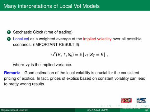
Many interpretations of Local Vol Models
1 Stochastic Clock (time of trading)2 Local vol as a weighted average of the implied volatility over all possible
scenarios. (IMPORTANT RESULT!!!)
σ2(K ,T ,S0) = E [vT |ST = K ] ,
where vT is the implied variance.
Remark: Good estimation of the local volatility is crucial for the consistentpricing of exotics. In fact, prices of exotics based on constant volatility can leadto pretty wrong results.
Regularization of Local Vol c©J.P.Zubelli (IMPA)September 2, 2011 19 /
55

Problem Statement
Starting Point: Dupire forward equation [Dup94]
−∂T U +12
σ2(T ,K )K 2
∂2K U− (r −q)K ∂K U−qU = 0 , T > 0 , (5)
K = S0ey , τ = T − t , b = q− r , u(τ,y) = eqτU t,S(T ,K ) (6)
and
a(τ,y) =12
σ2(T − τ;S0ey ) , (7)
Set q = r = 0 for simplicity to get:
uτ = a(τ,y)(∂2y u−∂y u) (8)
and initial conditionu(0,y) = S0(1−ey )+ (9)
Regularization of Local Vol c©J.P.Zubelli (IMPA)September 2, 2011 20 /
55
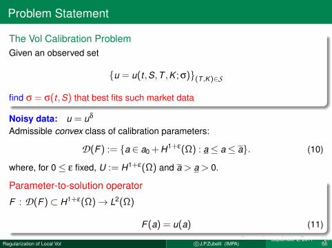
Problem Statement
The Vol Calibration ProblemGiven an observed set
u = u(t,S,T ,K ;σ)(T ,K )∈S
find σ = σ(t,S) that best fits such market data
Noisy data: u = uδ
Admissible convex class of calibration parameters:
D(F) := a ∈ a0 + H1+ε(Ω) : a≤ a≤ a. (10)
where, for 0≤ ε fixed, U := H1+ε(Ω) and a > a > 0.
Parameter-to-solution operator
F : D(F)⊂ H1+ε(Ω)→ L2(Ω)
F(a) = u(a) (11)
Regularization of Local Vol c©J.P.Zubelli (IMPA)September 2, 2011 21 /
55

LiteratureVery vast!!!
Avellaneda et al.[ABF+00, Ave98c, Ave98b,Ave98a, AFHS97]
Bouchev & Isakov [BI97]
Crepey [Cre03]
Derman et al. [DKZ96]
Egger & Engl [EE05]
Hofmann et al. [HKPS07, HK05]
Jermakyan [BJ99]
Achdou & Pironneau (2004)
Abken et al. (1996)
Ait Sahalia, Y & Lo, A (1998)
Berestycki et al. (2000)
Buchen & Kelly (1996)
Coleman et al. (1999)
Cont, Cont & Da Fonseca (2001)
Jackson et al. (1999)
Jackwerth & Rubinstein (1998)
Jourdain & Nguyen (2001)
Lagnado & Osher (1997)
Samperi (2001)
Stutzer (1997)
Regularization of Local Vol c©J.P.Zubelli (IMPA)September 2, 2011 22 /
55

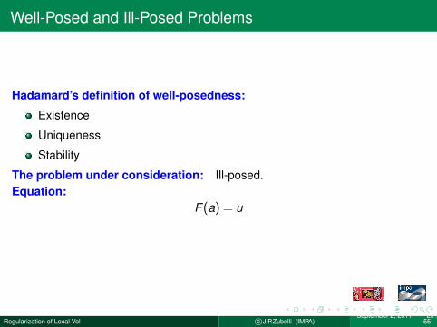
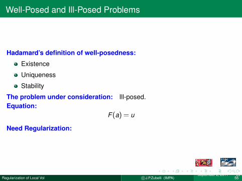
Well-Posed and Ill-Posed Problems
Hadamard’s definition of well-posedness:
Existence
Uniqueness
Stability
The problem under consideration: Ill-posed.Equation:
F(a) = u
Need Regularization:
Regularization of Local Vol c©J.P.Zubelli (IMPA)September 2, 2011 23 /
55
Well-Posed and Ill-Posed Problems
Hadamard’s definition of well-posedness:
Existence
Uniqueness
Stability
The problem under consideration: Ill-posed.Equation:
F(a) = u
Need Regularization:
Regularization of Local Vol c©J.P.Zubelli (IMPA)September 2, 2011 23 /
55
Well-Posed and Ill-Posed Problems
Hadamard’s definition of well-posedness:
Existence
Uniqueness
Stability
The problem under consideration: Ill-posed.Equation:
F(a) = u
Need Regularization:
Regularization of Local Vol c©J.P.Zubelli (IMPA)September 2, 2011 23 /
55
Regularization
Requirements:
Stability: Computed solution should depend continuously on data.Stability bounds for the solution.
Approximation: Computed solution should be close to the solution ofequation for noise-free data
Nonlinear Problems: Tikhonov regularization.Classical Theory: Add a quadratic regularization term.
Regularization of Local Vol c©J.P.Zubelli (IMPA)September 2, 2011 24 /
55
Approach
Theorem (Egger-Engel[EE05] Crepey[Cre03])The parameter to solution map
F : H1+ε(Ω)→ L2(Ω)
is
weak sequentialy continuous
compact and weakly closed
Consequences:
The inverse problem is ill-posed.
We can prove that the inverse problem satisfies the conditions to apply theregularization theory.
Regularization of Local Vol c©J.P.Zubelli (IMPA)September 2, 2011 25 /
55
Approach
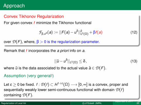
Convex Tikhonov RegularizationFor given convex f minimize the Tikhonov functional
Fβ,uδ(a) := ||F(a)−uδ||2L2(Ω) + βf (a) (12)
over D(F), where, β > 0 is the regularization parameter.
Remark that f incorporates the a priori info on a.
||u−uδ||L2(Ω) ≤ δ , (13)
where u is the data associated to the actual value a ∈D(F).
Assumption (very general!)
Let ε≥ 0 be fixed. f : D(f )⊂ H1+ε(Ω)−→ [0,∞] is a convex, proper andsequentially weakly lower semi-continuous functional with domain D(f )containing D(F).
Regularization of Local Vol c©J.P.Zubelli (IMPA)September 2, 2011 26 /
55
Approach
Convex Tikhonov RegularizationFor given convex f minimize the Tikhonov functional
Fβ,uδ(a) := ||F(a)−uδ||2L2(Ω) + βf (a) (12)
over D(F), where, β > 0 is the regularization parameter.
Remark that f incorporates the a priori info on a.
||u−uδ||L2(Ω) ≤ δ , (13)
where u is the data associated to the actual value a ∈D(F).
Assumption (very general!)
Let ε≥ 0 be fixed. f : D(f )⊂ H1+ε(Ω)−→ [0,∞] is a convex, proper andsequentially weakly lower semi-continuous functional with domain D(f )containing D(F).
Regularization of Local Vol c©J.P.Zubelli (IMPA)September 2, 2011 26 /
55
Questions
Questions:Does there exist a minimizer of the regularized problem?
Suppose that the noise level goes to zero... How fast does the regularizedgo to the true solution?
Regularization of Local Vol c©J.P.Zubelli (IMPA)September 2, 2011 27 /
55
Questions
Questions:Does there exist a minimizer of the regularized problem?
Suppose that the noise level goes to zero... How fast does the regularizedgo to the true solution?
Regularization of Local Vol c©J.P.Zubelli (IMPA)September 2, 2011 27 /
55

Questions
Questions:Does there exist a minimizer of the regularized problem?
Suppose that the noise level goes to zero... How fast does the regularizedgo to the true solution?
Regularization of Local Vol c©J.P.Zubelli (IMPA)September 2, 2011 27 /
55
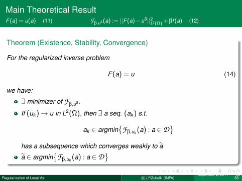
Main Theoretical ResultF(a) = u(a) (11) F
β,uδ(a) := ||F(a)−uδ||2L2(Ω) +βf (a) (12)
Theorem (Existence, Stability, Convergence)
For the regularized inverse problem
F(a) = u (14)
we have:
∃ minimizer of Fβ,uδ .
If (uk )→ u in L2(Ω), then ∃ a seq. (ak ) s.t.
ak ∈ argmin
Fβ,uk (a) : a ∈D
has a subsequence which converges weakly to a
a ∈ argmin
Fβ,uk (a) : a ∈D
Regularization of Local Vol c©J.P.Zubelli (IMPA)September 2, 2011 28 /
55
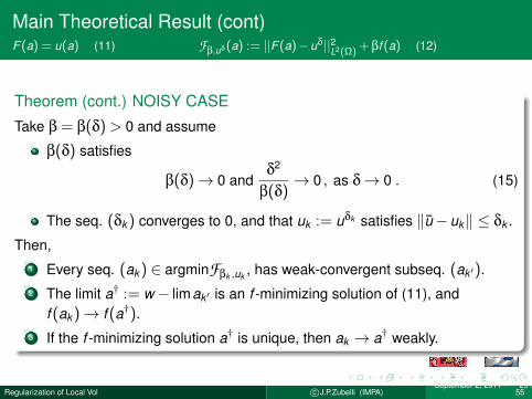
Main Theoretical Result (cont)F(a) = u(a) (11) F
β,uδ(a) := ||F(a)−uδ||2L2(Ω) +βf (a) (12)
Theorem (cont.) NOISY CASE
Take β = β(δ) > 0 and assume
β(δ) satisfies
β(δ)→ 0 andδ2
β(δ)→ 0 , as δ→ 0 . (15)
The seq. (δk ) converges to 0, and that uk := uδk satisfies ‖u−uk‖ ≤ δk .
Then,1 Every seq. (ak ) ∈ argminFβk ,uk , has weak-convergent subseq. (ak ′).2 The limit a† := w− limak ′ is an f -minimizing solution of (11), and
f (ak )→ f (a†).3 If the f -minimizing solution a† is unique, then ak → a† weakly.
Regularization of Local Vol c©J.P.Zubelli (IMPA)September 2, 2011 29 /
55

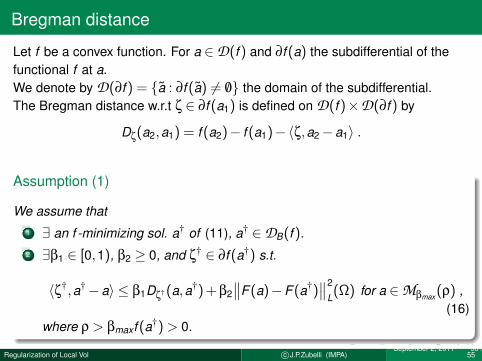
Bregman distance
Let f be a convex function. For a ∈D(f ) and ∂f (a) the subdifferential of thefunctional f at a.We denote by D(∂f ) = a : ∂f (a) 6= /0 the domain of the subdifferential.The Bregman distance w.r.t ζ ∈ ∂f (a1) is defined on D(f )×D(∂f ) by
Dζ(a2,a1) = f (a2)− f (a1)−〈ζ,a2−a1〉 .
Assumption (1)
We assume that1 ∃ an f -minimizing sol. a† of (11), a† ∈DB(f ).2 ∃β1 ∈ [0,1), β2 ≥ 0, and ζ† ∈ ∂f (a†) s.t.
〈ζ†,a†−a〉 ≤ β1Dζ†(a,a†) + β2∥∥F(a)−F(a†)
∥∥2
L(Ω) for a ∈Mβmax(ρ) ,
(16)where ρ > βmaxf (a†) > 0.
Regularization of Local Vol c©J.P.Zubelli (IMPA)September 2, 2011 30 /
55
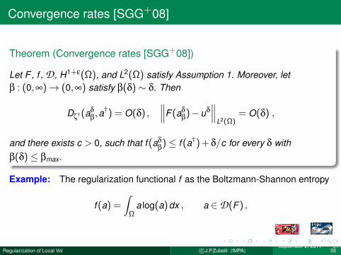
Convergence rates [SGG+08]
Theorem (Convergence rates [SGG+08])
Let F , f , D , H1+ε(Ω), and L2(Ω) satisfy Assumption 1. Moreover, letβ : (0,∞)→ (0,∞) satisfy β(δ)∼ δ. Then
Dζ†(aδ
β,a†) = O(δ) ,
∥∥∥F(aδ
β)−uδ
∥∥∥L2(Ω)
= O(δ) ,
and there exists c > 0, such that f (aδ
β)≤ f (a†) + δ/c for every δ with
β(δ)≤ βmax.
Example: The regularization functional f as the Boltzmann-Shannon entropy
f (a) =∫
Ωa log(a)dx , a ∈D(F) ,
Regularization of Local Vol c©J.P.Zubelli (IMPA)September 2, 2011 31 /
55

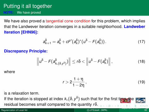
Putting it all togetherNOTE: We have proved
We have also proved a tangential cone condition for this problem, which impliesthat the Landwever iteration converges in a suitable neighborhood. LandweberIteration [EHN96]:
aδk+1 = aδ
k + cF ′(aδk )∗(uδ−F(aδ
k )) . (17)
Discrepancy Principle:∥∥∥uδ−F(aδ
k∗(δ,yδ))∥∥∥ ≤ rδ <
∥∥∥uδ−F(aδk )∥∥∥ , (18)
where
r > 21 + η
1−2η, (19)
is a relaxation term.If the iteration is stopped at index k∗(δ,yδ) such that for the first time, theresidual becomes small compared to the quantity rδ.
Regularization of Local Vol c©J.P.Zubelli (IMPA)September 2, 2011 32 /
55
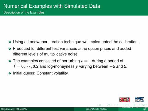
Numerical Examples with Simulated DataDescription of the Examples
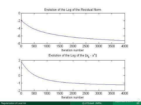
Using a Landweber iteration technique we implemented the calibration.
Produced for different test variances a the option prices and addeddifferent levels of multiplicative noise.
The examples consisted of perturbing a = 1 during a period ofT = 0, · · · ,0.2 and log-moneyness y varying between −5 and 5.
Initial guess: Constant volatility.
Regularization of Local Vol c©J.P.Zubelli (IMPA)September 2, 2011 33 /
55
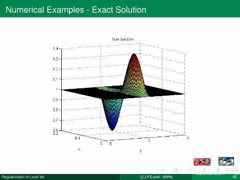
Numerical Examples - Exact Solution
Regularization of Local Vol c©J.P.Zubelli (IMPA)September 2, 2011 34 /
55
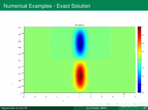
Numerical Examples - Exact Solution
Regularization of Local Vol c©J.P.Zubelli (IMPA)September 2, 2011 35 /
55

Numerical Examples 1 - noiseless - 4000 steps
Regularization of Local Vol c©J.P.Zubelli (IMPA)September 2, 2011 36 /
55

Numerical Examples 1 - error - 100 steps
Regularization of Local Vol c©J.P.Zubelli (IMPA)September 2, 2011 37 /
55
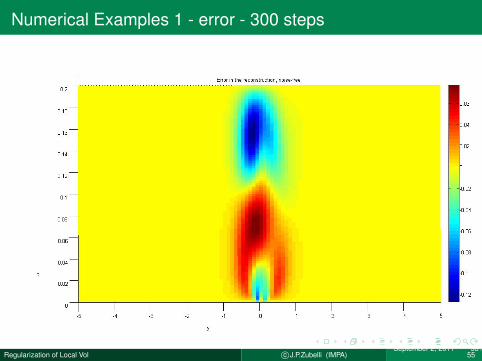
Numerical Examples 1 - error - 300 steps
Regularization of Local Vol c©J.P.Zubelli (IMPA)September 2, 2011 38 /
55

Numerical Examples 1 - error - 500 steps
Regularization of Local Vol c©J.P.Zubelli (IMPA)September 2, 2011 39 /
55
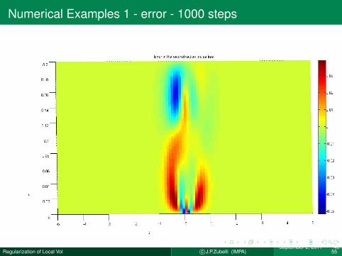
Numerical Examples 1 - error - 1000 steps
Regularization of Local Vol c©J.P.Zubelli (IMPA)September 2, 2011 40 /
55
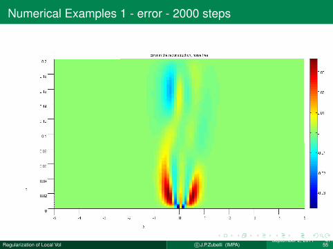
Numerical Examples 1 - error - 2000 steps
Regularization of Local Vol c©J.P.Zubelli (IMPA)September 2, 2011 41 /
55

Numerical Examples 1 - error - 4000 steps
Regularization of Local Vol c©J.P.Zubelli (IMPA)September 2, 2011 42 /
55
Regularization of Local Vol c©J.P.Zubelli (IMPA)September 2, 2011 43 /
55
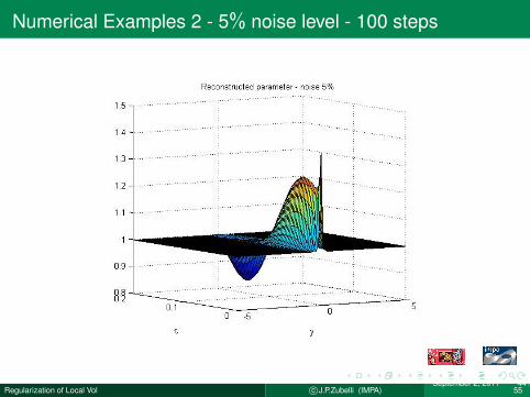
Numerical Examples 2 - 5% noise level - 100 steps
Regularization of Local Vol c©J.P.Zubelli (IMPA)September 2, 2011 44 /
55

Numerical Examples 2 - 5% noise level - 200 steps
Regularization of Local Vol c©J.P.Zubelli (IMPA)September 2, 2011 45 /
55
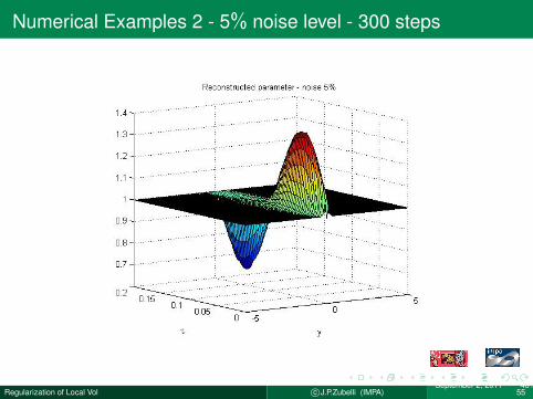
Numerical Examples 2 - 5% noise level - 300 steps
Regularization of Local Vol c©J.P.Zubelli (IMPA)September 2, 2011 46 /
55
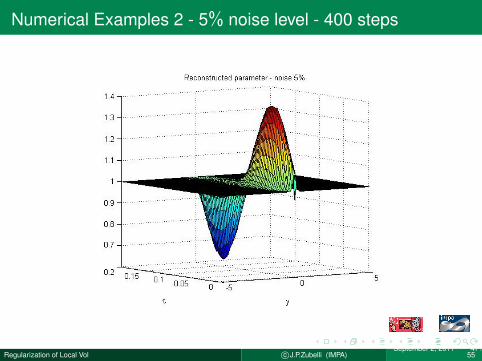
Numerical Examples 2 - 5% noise level - 400 steps
Regularization of Local Vol c©J.P.Zubelli (IMPA)September 2, 2011 47 /
55

Numerical Examples 2 - 5% noise level - Stopping criteria
Regularization of Local Vol c©J.P.Zubelli (IMPA)September 2, 2011 48 /
55

Regularization of Local Vol c©J.P.Zubelli (IMPA)September 2, 2011 49 /
55

Regularization of Local Vol c©J.P.Zubelli (IMPA)September 2, 2011 50 /
55

Numerical Examples 2 - 5% noise level - 2000 iterationsToo many!!!
Regularization of Local Vol c©J.P.Zubelli (IMPA)September 2, 2011 51 /
55

Numerical Examples: with Real DataReconstruction of a = σ2/2 with PBR Stock Data (implemented by Vinicius L. Albani/IMPA)
Figure: Minimal Entropy functional / Landweber Method / a priori Implied Vol /maturities: 2010-11
Regularization of Local Vol c©J.P.Zubelli (IMPA)September 2, 2011 52 /
55
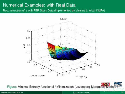
Numerical Examples: with Real DataReconstruction of a with PBR Stock Data (implemented by Vinicius L. Albani/IMPA)
Figure: Minimal Entropy functional / Minimization (Levenberg-Marquadt) Method /
Regularization of Local Vol c©J.P.Zubelli (IMPA)September 2, 2011 53 /
55

Conclusions
The problem of volatility surface calibration is a classical and fundamentalone in Quantitative Finance
Unifying framework for the regularization that makes use of tools fromInverse Problem theory and Convex Analysis.
Establishing convergence and convergence-rate results.
Obtain convergence of the regularized solution with respect to the noiselevel in L1(Ω)
The connection with exponential families opens the door to recent workson entropy-based estimation methods.
The connection with convex risk measures required the use of techniquesfrom Malliavin calculus.
Implemented a Landweber type calibration algorithm.
.
Regularization of Local Vol c©J.P.Zubelli (IMPA)September 2, 2011 54 /
55
THANK YOU FOR YOUR ATTENTION!!!
Collaborators:V. Albani (IMPA), A. de Cezaro (FURG), O. Scherzer (Vienna)
Regularization of Local Vol c©J.P.Zubelli (IMPA)September 2, 2011 55 /
55
M. Avellaneda, R. Buff, C. Friedman, N. Grandchamp, L. Kruk, andJ. Newman.Weighted Monte Carlo: A new technique for calibrating asset-pricingmodels.Spigler, Renato (ed.), Applied and industrial mathematics, Venice-2, 1998.Selected papers from the ‘Venice-2/Symposium’, Venice, Italy, June 11-16,1998. Dordrecht: Kluwer Academic Publishers. 1-31 (2000)., 2000.
M. Avellaneda, C. Friedman, R. Holmes, and D. Samperi.Calibrating volatility surfaces via relative-entropy minimization.Appl. Math. Finance, 4(1):37–64, 1997.
M. Avellaneda.Minimum-relative-entropy calibration of asset-pricing models.International Journal of Theoretical and Applied Finance, 1(4):447–472,1998.
Marco Avellaneda.The minimum-entropy algorithm and related methods for calibratingasset-pricing model.
Regularization of Local Vol c©J.P.Zubelli (IMPA)September 2, 2011 55 /
55
In Trois applications des mathematiques, volume 1998 of SMF Journ.Annu., pages 51–86. Soc. Math. France, Paris, 1998.
Marco Avellaneda.The minimum-entropy algorithm and related methods for calibratingasset-pricing models.In Proceedings of the International Congress of Mathematicians, Vol. III(Berlin, 1998), number Extra Vol. III, pages 545–563 (electronic), 1998.
I. Bouchouev and V. Isakov.The inverse problem of option pricing.Inverse Problems, 13(5):L11–L17, 1997.
James N. Bodurtha, Jr. and Martin Jermakyan.Nonparametric estimation of an implied volatility surface.Journal of Computational Finance, 2(4), Summer 1999.
S. Crepey.Calibration of the local volatility in a generalized Black-Scholes modelusing Tikhonov regularization.SIAM J. Math. Anal., 34(5):1183–1206 (electronic), 2003.
Regularization of Local Vol c©J.P.Zubelli (IMPA)September 2, 2011 55 /
55
Emanuel Derman, Iraj Kani, and Joseph Z. Zou.The local volatility surface: Unlocking the information in index optionprices.Financial Analysts Journal, 52(4):25–36, 1996.
B. Dupire.Pricing with a smile.Risk, 7:18– 20, 1994.
H. Egger and H. W. Engl.Tikhonov regularization applied to the inverse problem of option pricing:convergence analysis and rates.Inverse Problems, 21(3):1027–1045, 2005.
H. W. Engl, M. Hanke, and A. Neubauer.Regularization of inverse problems, volume 375 of Mathematics and itsApplications.Kluwer Academic Publishers Group, Dordrecht, 1996.
B. Hofmann and R. Kramer.
Regularization of Local Vol c©J.P.Zubelli (IMPA)September 2, 2011 55 /
55
On maximum entropy regularization for a specific inverse problem ofoption pricing.J. Inverse Ill-Posed Probl., 13(1):41–63, 2005.
B. Hofmann, B. Kaltenbacher, C. Poschl, and O. Scherzer.A convergence rates result for Tikhonov regularization in Banach spaceswith non-smooth operators.Inverse Problems, 23(3):987–1010, 2007.
O. Scherzer, M. Grasmair, H. Grossauer, M. Haltmeier, and F. Lenzen.Variational Methods in Imaging, volume 167 of Applied MathematicalSciences.Springer, New York, 2008.
Regularization of Local Vol c©J.P.Zubelli (IMPA)September 2, 2011 55 /
55