Non-parametric transformation regression with non-stationary data

Oliver Linton Qiying Wang

The Institute for Fiscal Studies Department of Economics, UCL

cemmap working paper CWP16/13

Non-parametric transformation regression withnon-stationary data

Oliver Linton∗

University of CambridgeQiying Wang†

University of Sydney

April 22, 2013

Abstract

We examine a kernel regression smoother for time series that takes account ofthe error correlation structure as proposed by Xiao et al. (2008). We show that thismethod continues to improve estimation in the case where the regressor is a unitroot or near unit root process.

Key words and phrases: Dependence; Effi ciency; Cointegration; Non-stationarity;Non-parametric estimation.

JEL Classification: C14, C22.

1 Introduction

This paper is concerned with estimation of a nonstationary nonparametric cointegrat-

ing regression. The theory of linear cointegration is extensive and originates with the

work of Engle and Granger (1987), see also Stock (1987), Phillips (1991), and Johanssen

(1988). Wang and Phillips (2009a, b, 2011) recently considered the nonparametric coin-

tegrating regression. They analyse the behaviour of the standard kernel estimator of

the cointegrating relation/nonparametric regression when the covariate is nonstationary.

They showed that the under self (random) normalization, the estimator is asymptotically

normal. See also Phillips and Park (1998), Karlsen and Tjostheim (2001), Karlsen, et

al.(2007), Schienle (2008) and Cai, et al.(2009).

∗Address: Faculty of Economics, Austin Robinson Building, Sidgwick Avenue, Cambridge, CB3 9DD,UK. Email: obl20@cam.ac.uk. I would like to thank the European Research Council for financial support.†Address: School of Mathematics and Statistics, The University of Sydney, NSW 2006, Australia.

E-mail: qiying@maths.usyd.edu.au. This author thanks the Australian Research Council for financialsupport.

1

We extend this work by investigating an improved estimator in the case where there

is autocorrelation in the error term. Standard kernel regression smoothers do not take

account of the correlation structure in the covariate xt or the error process ut and es-

timate the regression function in the same way as if these processes were independent.

Furthermore, the variance of such estimators is proportional to the short run variance

of ut, σ2u = var(ut) and does not depend on the regressor or error covariance functions

γx(j) = cov(xt, xt−j), γu(j) = cov(ut, ut−j), j 6= 0. Although the time series properties

do not effect the asymptotic variance of the usual estimators, the error structure can be

used to construct a more effi cient estimator. Xiao, Linton, Carroll, and Mammen (2003)

proposed a more effi cient estimator of the regression function based on a prewhitening

transformation. The transform implicitly takes account of the autocorrelation structure.

They obtained an improvement in terms of variance over the usual kernel smoothers. Lin-

ton and Mammen (2006) proposed a type of iterated version of this procedure and showed

that it obtained higher effi ciency. Both these contributions assumed that the covariate

process was stationary and weakly dependent. We consider here the case where xt is

nonstationary, of the unit root or close to unit root type. We allow the error process to

have some short term memory, which is certainly commonplace in the linear cointegration

literature. We show that the Xiao, Linton, Carroll, and Mammen (2003) procedure can

improve effi ciency even in this case and one still obtains asymptotic normality for the self

normalized estimator, which allows standard inference methods to be applied. In order

to establish our results we require a new strong approximation result and use this to

establish the L2 convergence rate of the usual kernel estimator.

2 The model and main results

Consider a non-linear cointegrating regression model:

yt = m(xt) + ut, t = 1, 2, ..., n, (2.1)

where ut = ρut−1 + εt with |ρ| < 1 and xt is a non-stationary regressor. The conventional

kernel estimator of m(x) is defined as

m(x) =

∑ns=1 ysK[(xs − x)/h]∑ns=1K[(xs − x)/h]

,

where K(x) is a nonnegative real function and the bandwidth parameter h ≡ hn → 0 as

n→∞.

2

On the other hand, we may write the model (2.1) as

yt−1 = m(xt−1) + ut−1, (2.2)

yt − ρyt−1 + ρm(xt−1) = m(xt) + εt. (2.3)

It is expected that a two-step estimator of m(x) by using models (2.2) and (2.3) may

achieve effi ciency improvements over the usual estimator m(x) by (2.1).

The strategy to provide the two-step estimator is as follows:

Step 1: Construct an estimator of m(x), say m1(x), by using model (2.2). This can

be the conventional kernel estimator defined by

m1(x) =

∑ns=2 ys−1K[(xs−1 − x)/h]∑n

s=2K[(xs−1 − x)/h],

where K(x) is a nonnegative real function and the bandwidth parameter h ≡ hn → 0 as

n→∞.Step 2: Construct an estimator of ρ by

ρ =

∑ns=2 usus−1∑ns=2 u

2s−1

.

Note that ρ is a LS estimator from model:

ut = ρut−1 + εt,

where ut = yt − m1(xt).

Step 3: Construct an estimator ofm(x), say m2(x), by using (2.3) and kernel method,

but instead of the left hand m(x) in model (2.3) by m1(x).

We now have a two-step estimator m2(x) of m(x), defined as follows:

m2(x) =

∑nt=1

[yt − ρyt−1 + ρm1(xt−1)

]K[(xt − x)/h]∑n

t=1K[(xt − x)/h].

To establish our claim, that is, m2(x) achieves effi ciency improvements over the usual

estimator m(x), we make the following assumptions.

Assumption 2.1. xt = λxt−1 + ξt, (x0 ≡ 0), where λ = 1 + τ/n with τ being a

constant and ξj, j ≥ 1 is a linear process defined by

ξj =∞∑k=0

φk νj−k, (2.4)

3

where φ0 6= 0, φ ≡∑∞

k=0 φk 6= 0 and∑∞

k=0 |φk| < ∞ , and where νj,−∞ < j < ∞ isa sequence of iid random variables with Eν0 = 0, Eν20 = 1, E|ν0|2+δ <∞ for some δ > 0

and characteristic function ϕ(t) of ν0 satisfies∫∞−∞(1 + |t|) |ϕ(t)|dt <∞.

Assumption 2.2. ut = ρut−1 + εt with |ρ| < 1 and ε0 = u0 = 0, where Fn,t =

σ(ε0, ε1, ..., εt, x1, ..., xn) and εt,Fn,tnt=1 forms a martingale difference sequence satisfying,as n→∞ first and then m→∞,

maxm≤t≤n

|E(ε2t |Fn,t−1)− σ2| → 0, a.s.,

where σ2 is a given constant, and sup 1≤t≤nn≥1

E(|εt|q|Fn,t−1) <∞ a.s. for some q > 2.

Assumption 2.3. (a)∫∞−∞K(s)ds = 1 and K(·) has a compact support; (b) For any

x, y ∈ R, |K(x)−K(y)| ≤ C |x− y|, where C is a positive constant; (c) For p ≥ 2,∫ypK(y)dy 6= 0,

∫yiK(y)dy = 0, i = 1, 2, ..., p− 1.

Assumption 2.4. (a) There exist a 0 < β ≤ 1 and α ≥ 0 such that

|m(x+ y)−m(x)| ≤ C (1 + |x|α) |y|β,

for any x ∈ R and y suffi ciently small, where C is a positive constant; (b) For given fixedx, m(x) has a continuous p + 1 derivatives in a small neighborhood of x, where p ≥ 2 is

defined as in Assumption 2.3(c).

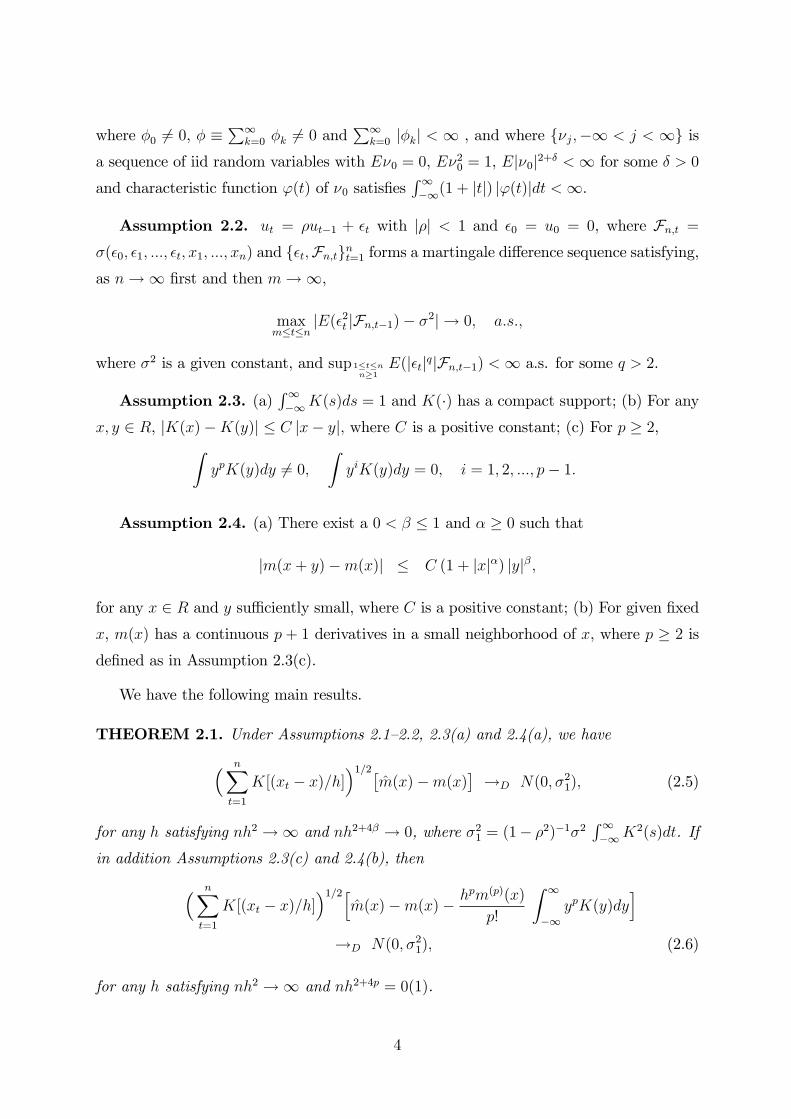
We have the following main results.

THEOREM 2.1. Under Assumptions 2.1—2.2, 2.3(a) and 2.4(a), we have( n∑t=1

K[(xt − x)/h])1/2[

m(x)−m(x)]→D N(0, σ21), (2.5)

for any h satisfying nh2 →∞ and nh2+4β → 0, where σ21 = (1− ρ2)−1σ2∫∞−∞K

2(s)dt. If

in addition Assumptions 2.3(c) and 2.4(b), then( n∑t=1

K[(xt − x)/h])1/2[

m(x)−m(x)− hpm(p)(x)

p!

∫ ∞−∞

ypK(y)dy]

→D N(0, σ21), (2.6)

for any h satisfying nh2 →∞ and nh2+4p = 0(1).

4

THEOREM 2.2. Under Assumptions 2.1—2.2, 2.3(a)—(b), 2.4(a) and∑∞

i=0 i|φi| < ∞,we have

|ρ− ρ| = OP

nα/2hβ + (nh2)−1/4

, (2.7)

and with σ22 = σ2∫∞−∞K

2(s)dt,

( n∑t=1

K[(xt − x)/h])1/2 [

m2(x)−m(x)]→D N(0, σ22), (2.8)

for any h satisfying that nh2+4β → 0, nαh2β → 0 and n1−ε0h2 → ∞ for some ε0 > 0. If

in addition Assumptions 2.3(c) and 2.4(b), then( n∑t=1

K[(xt − x)/h])1/2[

m2(x)−m(x)− hpm(p)(x)

p!

∫ ∞−∞

ypK(y)dy]

→D N(0, σ22), (2.9)

for any h satisfying that nh2+4p = O(1), nαh2β → 0 and n1−ε0h2 →∞ for some ε0 > 0.

Remark 1. Theorem 2.1 generalizes the related results in previous articles. See, for

instance, Wang and Phillips (2009a, 2011), where the authors investigated the asymptotics

under ρ = 0 and τ = 0. As noticed in previous works, the conditions to establish

our results are quite weak, in particular, a wide range of regression function m(x) is

included in Assumption 2.4(a), like m(x) = 1/(1 + θ |x|β), m(x) = (a+ bex)/(1 + ex) and

m(x) = θ1 + θ2x+ ...+ θkxk−1.

Remark 2. As |ρ| < 1, Theorem 2.2 confirms the claim that m2(x) achieves effi ciency

improvements over the usual estimator m(x) under certain additional conditions on m(x)

and the bandwidth h. Among these additional conditions, the requirement on the band-

width h (that is, nαh2β → 0 and n1−ε0h2 →∞, where ε0 can be suffi ciently small) implythat 0 ≤ α < β, which in turn requires that the rate of m(x) divergence to ∞ on the tail

is not fast than |x|1+β. In comparison to Theorem 2.1, this is a little bit restrictive but

it is reasonable, due to the fact that the consistency result (2.7) heavily depend on the

following convergence for the kernel estimator m(x):

1

n

n∑t=1

[m(xt)−m(xt)

]2(2.10)

as n → ∞. As xt ∼√t under our model, it is natural for the restriction on the tail of

m(x) to enable (2.10). The result (2.10) is a consequence of Theorem 3.1 in next section,

which provides a strong approximation result on the convergence to a local time process.

5

3 Strong approximation to local time

This section investigates strong approximation to a local time process which essentially

provides a technical tool in the development of the uniform convergence such as (2.10)

for the kernel estimator m(x). As the condition imposed is different, this section can be

read separately.

Let xk,n, 1 ≤ k ≤ n, n ≥ 1 be a triangular array, constructed from some underlying

nonstationary time series and assume that there is a continuous limiting Gaussian process

G(t), 0 ≤ t ≤ 1, to which x[nt],n converges weakly, where [a] denotes the integer part of a.

In many applications, we let xk,n = d−1n xk where xk is a nonstationary time series, such

as a unit root or long memory process, and dn is an appropriate standardization factor.

This section is concerned with the limit behaviour of the statistic Sn(t), defined by

Sn(t) =cnn

n∑k=1

g[cn (xk,n − x[nt],n)], t ∈ [0, 1], (3.1)

where cn is a certain sequence of positive constants and g is a real integrable function on

R. As noticed in last section and previous research [see, e.g., Wang and Phillips (2012)],

this kind of statistic appears in the inference for the unknown regression function m(x)

and its limit behaviour plays a key role in the related research fields.

The aim of this section is to provide a strong approximation result for the target

statistic. To achieve our aim, we make use of the following assumptions.

Assumption 3.1. supx |x|γ|g(x)| < ∞ for some γ > 1,∫∞−∞ |g(x)|dx < ∞ and

|g(x)− g(y)| ≤ C|x− y| whenever |x− y| is suffi ciently small on R.

Assumption 3.2. On a rich probability space, there exist a continuous local martin-

gale G(t) having a local time LG(t, s) and a sequence of stochastic processes Gn(t) such

that Gn(t); 0 ≤ t ≤ 1 =D G(t); 0 ≤ t ≤ 1 for each n ≥ 1 and

sup0≤t≤1

|x[nt],n −Gn(t)| = oa.s.(n−δ0). (3.2)

for some 0 < δ0 < 1.

Assumption 3.3. For all 0 ≤ j < k ≤ n, n ≥ 1, there exist a sequence of σ-fields

Fk,n (define F0,n = σφ,Ω, the trivial σ-field) such that,(i) xj,n are adapted to Fj,n and, conditional on Fj,n, [n/(k − j)]d(xk,n − xj,n) where

0 < d < 1, has a density hk,j,n(x) satisfying that hk,j,n(x) is uniformly bounded by a

constant K and

6

(ii) supu∈R∣∣hk,j,n(u+t)−hk,j,n(u)

∣∣ ≤ C min|t|, 1, whenever n and k−j are suffi cientlylarge and t ∈ R.

Assumption 3.4. There is a ε0 > 0 such that cn →∞ and n−1+ε0cn → 0.

The following is our main result.

THEOREM 3.1. Suppose Assumptions 3.1—3.4 hold. On the same probability space as

in Assumption 3.2, for any l > 0, we have

sup0≤t≤1

|Sn(t)− τ Lnt| = oP (log−l n) (3.3)

where τ =∫∞−∞ g(t)dt and Lnt = limε→0

12ε

∫ 10I(|Gn(s)−Gn(t)| ≤ ε)ds.

Due to technical diffi culty, the rates in (3.3) may not be optimal, which, in our guess,

should have the form n−δ1 , where δ1 > 0 is related to δ0 > 0 given in Assumption 3.2.

However, by noting Lnt; 0 ≤ t ≤ 1 =D LG(1, G(t)); 0 ≤ t ≤ 1 1 due to Gn(t); 0 ≤ t ≤1 =D G(t); 0 ≤ t ≤ 1, the result (3.3) is enough in many applications. To illustrate,we have the following theorem which provides the lower bound of Sn(t) over t ∈ [0, 1]. As

a consequence, we establish the result (2.10) when xt satisfies Assumption 2.1.

THEOREM 3.2. Let xt be defined as in Assumption 2.1 with∑∞

k=0 k|φk| < ∞. LetAssumptions 2.3(a)—(b) hold. Then, for any η > 0 and fixed M0 > 0, there exist M1 > 0

and n0 > 0 such that

P(

infs=1,2,...,n

n∑t=1

K[(xt − xs)/h] ≥√nh/M1

)≥ 1− η, (3.4)

for all n ≥ n0 and h satisfying that h → 0 and n1−ε0h2 → ∞ for some ε0 > 0. Conse-

quently, we have

Vn :=1

n

n∑t=1

[m(xt)−m(xt)

]2= OP

nαh2β + (nh2)−1/2

, (3.5)

that is, (2.10) holds true if in addition nαh2β → 0.

1Here and belew, we define LG(1, x) = limε→012ε

∫ 10I(|G(s) − x| ≤ ε)ds, a local time process of the

G(s) whenever it exists.

7

4 Extension

We next propose another estimator that potentially can improve the effi ciency even more.

Following Linton and Mammen (2008), we obtain

m(x) =1

1 + ρ2[E(Z−t (ρ)|xt = x)− ρE(Z+t (ρ)|xt−1 = x)

]=

1

1 + ρ2E[Z−t (ρ)− ρZ+t+1(ρ)|xt = x

]Z−t (ρ) = yt − ρyt−1 + ρm(xt−1)

Z+t (ρ) = yt − ρyt−1 −m(xt).

Let m(.), ρ be initial consistent estimators, and let

Z−t (ρ) = yt − ρyt−1 + ρm(xt−1)

Z+t (ρ) = yt − ρyt−1 − m(xt).

Then let

meff (x) =1

1 + ρ2E[Z−t (ρ)− ρZ+t+1(ρ)|xt = x

].

We claim that the following result holds. The proof is similar to earlier results and is

ommitted.

THEOREM 4.1. If in addition to Assumptions 2.1-2.4,∑∞

i=0 i|φi| <∞. Then, for anyh satisfying nh2 log−4 n→∞ and nh2+4β → 0, we have

( n∑t=1

K[(xt − x)/h])1/2 [

m2(x)−m(x)]→D N(0, σ23)

where σ22 = (1 + ρ2)−1∫∞−∞K

2(s)dt.

We have σ23 ≤ σ22 ≤ σ21, and so meff (x) is more effi cient (according to asymptotic

variance) than m2(x), which itself is more effi cient than m(x).

5 Monte Carlo Simulation

We investigate the performance of our procedure on simulated data. We chose a similar

design to Wang and Phillips (2009b) except we focus on error autocorrelation rather than

contemporaneous endogeneity. We suppose that

yt = m(xt) + σut, ut = ρ0ut−1 + εt

8

with m(x) = x and m(x) = sin(x), where xt = xt−1 + ηt, with ηt ∼ N(0, 1), σ = 0.2, and

εt ∼ N(0, 1). We used the Epanechnikov kernel for estimation with the bandwidth n−bc.

We examine a range of values of ρ0 and the bandwidth constant bc, which are given below.

We consider n = 500, 1000 and take ns = 1000 replications. We report the performance

measure1

K

K∑k=1

|m(xk)−m(xk)|2 ,

where K = 101 and xk = −1,−0.98, . . . ., 1. The results for the linear case are givenbelow in Tables 1-2. The results show that there is an improvement when going from

n = 500 to n = 1000 and when going from m1 to m2. In the linear case, the bigger the

bandwidth the better. In the cubic case (not shown), smaller bandwidths do better as

the bias issue is much more severe in this case.

*** Tables 1-2 here ***

We show in Tables 3 and 4 the performance of the estimator of ρ for n = 500 and

n = 1000. This varies with bandwidth and is generally quite poor, although improves

with sample size. Finally, we give some indication of the distributional approximation.

In Figure 1 we show the QQ plot for our (standardized) estimator m2 in the case where

m(x) = sin(x), ρ = 0.95, n = 1000, and bc = 1/10.

6 Proofs

Section 6.1 provides several preliminary lemmas. Some of them are are of independent

interests. The proofs of main theorems will be given in Sections 6.2-6.4.

6.1 Preliminary lemmas

First note that

xt =t∑

j=1

λt−j ξj =

t∑j=1

λt−jj∑

i=−∞νiφj−i

= λt−s xs +

t∑j=s+1

λt−js∑

i=−∞νiφj−i +

t∑j=s+1

λt−jj∑

i=s+1

νiφj−i

:= λt−s xs + ∆s,t + x′s,t, (6.1)

9

where

x′s,t =

t−s∑j=1

λt−j−sj∑i=1

νi+sφj−i =

t∑i=s+1

νi

t−i∑j=0

λt−j−i φj.

Write d2s,t =∑t

i=s+1 λ2(t−i)(

∑t−ij=0 λ

−jφj)2 = E(x′s,t)

2. Recall limn→∞ λn = eτ and limn→∞ λ

m =

1 for any fixed m. The routine calculations show that, whenever n is suffi ciently large,

e−|τ |/2 ≤ λk ≤ 2e|τ |, for all −n ≤ k ≤ n (6.2)

and there exist γ1, γ0 > 0 such that

γ0 ≤ infn≥k≥m

|k∑j=0

λ−jφj| ≤ γ1, (6.3)

whenever n,m are suffi ciently large. By virtue of (6.2)-(6.3), it is readily seen that ds,t 6= 0

for all 0 ≤ s < t ≤ n because φ =∑∞

j=0 φj 6= 0 and C1(t − s) ≤ d2s,t ≤ C2(t − s).

Consequently,

1√t−sx

′s,t has a density hs,t(x), (6.4)

which is uniformly bounded by a constant C0 and∫∞−∞(1 + |u|)|ϕs,t(u)|du <∞ uniformly

for 0 ≤ s < t ≤ n, where ϕs,t(u) = Eeiux′s,t/√t−s, due to

∫(1 + |u|)|Eeiuν0 |dt < ∞. See

the proof of Corollary 2.2 in Wang and Phillips (2009a) and/or (7.14) and Proposition

7.2 (page 1934 there) of Wang and Phillips (2009b) with a minor modification. Hence,

conditional on Fk = σ(νj,−∞ < j ≤ k),

(xt − xs)/√t− s has a density h∗s,t(x) ≡ hs,t(x− x∗s,t/

√t− s) (6.5)

where x∗s,t = (λt−s − 1)xs + ∆s,t, satisfying, for any u ∈ R,

supx

∣∣h∗s,t(x+ u)− h∗s,t(x)∣∣ ≤ sup

x|hs,t(x+ u)− hs,t(x)|

≤ C∣∣∣ ∫ ∞−∞

(e−iv(x+u) − e−ivx

)ϕs,t(v)dv

∣∣∣≤ C min|u|, 1

∫ ∞−∞

(1 + |v|) |ϕs,t(v)|dv ≤ C1 min|u|, 1, (6.6)

where in the last second inequality of (6.6), we have used the inverse formula of the

characteristic function.

10

We also have the following presentation for the xt:

xt =t∑

j=1

λt−j ξj =

t∑j=1

λt−j( j−1∑i=0

+

∞∑i=j

)φiνj−i

=

t−1∑i=0

φi λt−i

t∑j=1

λ−jνj −t−1∑i=0

φi λt−i

t∑j=t−i+1

λ−jνj +

t∑j=1

λt−j∞∑i=0

φi+jν−i

= at x′t − x′′t + x′′′t , say, (6.7)

where at =∑t−1

i=0 φi λ−i, x′t =

∑tj=1 λ

t−jνj and

|x′′t |+ |x′′′t | ≤ C0t1/(2+δ), a.s. (6.8)

for some constant C0 > 0. Indeed, using (6.2) and strong law, we obtain that, for some

constant C0 > 0,

|x′′t | ≤ 2e|τ |t−1∑i=0

|φi|t∑

j=t−i+1|νj| ≤ 2e|τ | max

1≤j≤t|νj|

t−1∑i=0

i|φi|

≤ C t1/(2+δ)(1

t

t∑j=1

|νj|2+δ)1/(2+δ) ≤ C0t

1/(2+δ), a.s., (6.9)

since E|ν1|2+δ <∞ and∑∞

i=0 i|φi| <∞ . Note that∞∑j=1

j−1/(2+δ)E|∞∑i=0

φi+jν−i| ≤∞∑j=1

j−1/(2+δ)( ∞∑i=j

φ2i)1/2

≤ C∞∑j=1

j−1−1/(2+δ)( ∞∑i=j

i|φi|)1/2

<∞,

which yields that∑∞

j=1 j−1/(2+δ)|

∑∞i=0 φi+jν−i| < ∞, a.s. It follows from (6.2) again and

the Kronecker lemma that

|x′′′t | ≤ C

t∑j=1

∣∣ ∞∑i=0

φi+jν−i∣∣ = o(t1/(2+δ)), a.s. (6.10)

This proves (6.8).

We are now ready to provide several preliminary lemmas.

LEMMA 6.1. Suppose that p(x) satisfies∫|p(x)|dx < ∞ and Assumption 2.1 holds.

Then, for any h→ 0 and all 0 ≤ s < t ≤ n, we have

E(|p(xt/h)|

∣∣Fs) ≤ C0h√t− s

∫ ∞−∞|p(x+ xs/h)|dx

=C0h√t− s

∫ ∞−∞|p(x)|dx, a.s., (6.11)

where Fs = σνs, νs−1, ....

11

Proof. Recall (6.1), (6.5) and the independence of νk. The result (6.11) follows from

a routine calculation and hence the details are omitted. 2

LEMMA 6.2. Suppose that p(x) satisfies∫

[|p(x)| + p2(x)]dx < ∞ and∫p(x)dx 6= 0.

Suppose Assumption 2.1 holds. Then, for any h→ 0 and nh2 →∞,

φ√nh

n∑t=1

p[(xt − x)/h

]→D

∫ ∞−∞

p(x)dxLG(1, 0), (6.12)

where G(t) = W (t) + κ∫ t0eκ(t−s)W (s)ds with W (s) being a standard Brownian motion

and LG(r, x) is a local time of the Gaussian process G(t).

Proof. This is a corollary of Theorem 3.1 of Wang and Phillips (2009a). The

inspection on the conditions is similar to Proposition 7.2 of Wang and Phillips (2009b).

We omit the details. 2

LEMMA 6.3. Suppose Assumptions 2.1-2.2 and 2.3(a) hold. Then, for any h→ 0 and

nh2 →∞,n∑t=1

utZnt →D N(0, σ21), (6.13)

where Znt = K[(xt− x)/h]/(∑n

t=1K[(xt− x)/h])1/2

and σ21 = (1− ρ2)−1σ2∫∞−∞K

2(x)dx.

Proof. For the notation convenience, we assume σ2 = 1 in the following proof. Note

that ut =∑t

k=1 ρt−kεk. We have

∑nt=1 utZnt =

∑nk=1 εkZ

∗nk, where Z

∗nk =

∑nt=k ρ

t−kZnt.

We first claim thatn∑k=1

Z2nk →P

∫ ∞−∞

K2(x)dx, (6.14)

n∑k=1

Z∗2nk →P (1− ρ2)−1∫ ∞−∞

K2(x)dx. (6.15)

The proof of (6.14) is simple by applying Lemma 6.2. To see (6.15), note thatn∑k=1

Z∗2nk = Λ−1n

n∑k=1

( n∑t=k

ρt−kK[(xt − x)/h])2

= Λ−1n

n∑k=1

n∑t=k

ρ2(t−k)K2[(xt − x)/h] + Λ−1n Γ1n

= (1− ρ2)−1n∑k=1

Z2nk + Λ−1n (Γ1n − Γ2n) [by (6.14)]

= (1− ρ2)−1∫ ∞−∞

K2(x)dx+ Λ−1n (Γ1n − Γ2n) + oP (1), (6.16)

12

where Λn =∑n

t=1K[(xt − x)/h],

Γ1n = 2n∑k=1

∑k≤s<t≤n

ρs−k ρt−kK[(xs − x)/h]K[(xt − x)/h],

Γ2n = (1− ρ2)−1n∑t=1

K2[(xt − x)/h] ρ2t.

Note that Λn/(√nh) →D φ−1 LG(1, 0) by Lemma 6.2. The result (6.15) will follow if we

prove

Γ1n + Γ2n = oP [(nh2)1/2]. (6.17)

Recall K(x) ≤ C and |ρ| < 1. It is readily seen that Γ2n ≤ C = oP [(nh2)1/2], due to

nh2 →∞. On the other hand, by applying Lemma 6.1, for any t > s, we have

EK[(xs − x)/h]K[(xt − x)/h]

≤ E

[K[(xs − x)/h]E

K[(xt − x)/h] | Fs

]≤ Ch√

t− sh√s.

It follows that

EΓ1n ≤ C h2n∑k=1

∑k≤s<t≤n

ρs−k ρt−k1√t− s

1√s

≤ C1h2

n∑k=1

1√k≤ Ch2

√n.

which implies that Γ1n = OP (h2√n) = oP [(nh2)1/2]. This proves (6.17) and hence the

claim (6.15).

We now turn to the proof of (6.13). Since, given x1, x2, ..., xn, the sequence (Z∗nk εk, k =

1, 2, ..., n) still forms a martingale difference by Assumption 2.2, it follows from Theorem

3.9 [(3.75) there] in Hall and Heyde (1980) with δ = q/2− 1 that

supx

∣∣P( n∑t=1

εtZ∗nt ≤ xσ1 | x1, x2, ..., xn

)− Φ(x)

∣∣ ≤ A(δ)L1/(1+q)n , a.s.,

where A(δ) is a constant depending only on q > 2 and

Ln =1

σq1

n∑k=1

|Z∗nk|qE(|εk|q | x1, ..., xn) + E∣∣∣ 1

σ21

n∑k=1

Z∗2nk[E(ε2k|Fk−1)− 1

]∣∣∣q/2 | x1, ..., xn.Recall that K(x) is uniformly bounded and

max1≤k≤n

|Z∗nk| ≤ C max1≤k≤n

|Znk| ≤ C/( n∑t=1

K[(xt − x)/h])1/2

= oP (1),

13

by Assumption 2.3 and Lemma 6.2. Routine calculations, together with (6.15), show that

Ln = oP (1),

since q > 2. Therefore the dominate convergence theorem yields that

supx

∣∣P( n∑t=1

utZnt ≤ xσ1)− Φ(x)

∣∣≤ E

[supx

∣∣P( n∑t=1

εtZ∗nt ≤ xσ1 | x1, x2, ..., xn

)− Φ(x)

∣∣]→ 0.

This completes the proof of Lemma 6.3. 2

LEMMA 6.4. Under Assumptions 2.3(a) and 2.4(a), for any x ∈ R, we have∣∣Λn(x)−m(x)∣∣ ≤ C (1 + |x|α)hβ, (6.18)

where Λn(x) =∑nt=1m(xt)K[(xt−x)/h]∑n

t=1K[(xt−x)/h]. If in addition Assumption 2.4(b), we have

∣∣Λn(x)−m(x)− hpm(p)(x)

p!

∫ ∞−∞

ypK(y)dy∣∣ = oP [(nh2)−1/4], (6.19)

whenever nh2 →∞ and nh2+4p = O(1), for any fixed x.

Proof. By Assumption 2.4(a) and the compactness of K(x), the result (6.18) is simple.

The proof of (6.19) is the same as in the proof of Theorem 2.2 in Wang and Phillips (2011).

We omit the details. 2

LEMMA 6.5. For any s, t ∈ R and ξ > 0, there exists a constant C such that

|LG(1, s)− LG(1, t)| ≤ C |s− t|1/2−ξ a.s., (6.20)

where G(x) is a continuous local martingale.

Proof. See Corollary 1.8 of Revuz and Yor (1994, p. 226). 2

LEMMA 6.6. Suppose that Assumptions 3.1-3.4 hold. Then, for any l > 0, we have

In := supt∈R

sups:|s−t|≤εn

∣∣∣cnn

n∑k=1

ft,s(xk,n)∣∣∣ = Oa.s.(log−l n) (6.21)

where εn ≤ cnn−l1 for some l1 > 0 and ft,s(x) = g(cnx+ t)− g(cnx+ s).

Proof. See Lemma 3.5 of Liu, Chan and Wang (2013). 2

14

6.2 Proofs of Theorem 2.1 and 2.2

We only prove Theorem 2.2. Using Lemmas 6.3 and 6.4, the proof of Theorem 2.1 is

standard [see, e.g., Wang and Phillips (2011)], and hence the details are omitted.

Start with (2.7). Recall that ut = yt − m1(xt) = ut + m(xt) − m1(xt). Simple

calculations show that

ρ− ρ =

∑ns=2(us − ρus−1)us−1∑n

s=2 u2s−1

=

∑ns=2 εs us−1∑ns=2 u

2s−1

+

∑ns=2 us−1

[m(xs)− m1(xs) + ρ m1(xs−1)−m(xs−1)

]∑ns=2 u

2s−1

:= R1n +R2n. (6.22)

As Vn = 1n

∑nt=1

[m1(xt)−m(xt)

]2= OP

nαh2β + (nh2)−1/2

by (3.5) of Theorem 3.2, it

follows from 1n

∑nt=1 u

2t → (1−ρ2)−1σ2, a.s., that 1

n

∑ns=2 u

2s−1 →P (1−ρ2)−1σ2, whenever

nαh2β → 0 and nh2 →∞. This, together with Hölder’s inequality, yields that

|R2n| ≤ 2(1 + ρ2)1/2V 1/2n /

( n∑s=2

u2s−1)1/2

= OP

nα/2hβ + (nh2)−1/4

.

On the other hand, by recalling Assumption 2.2, it is readily seen that R1n = OP (n−1/2).

Taking these facts into (6.22), we obtain (2.7).

We next prove (2.8). We may write

m2(x)−m(x) =ρ∑n

t=1

[m1(xt−1)−m(xt−1)

]K[(xt − x)/h]∑n

t=1K[(xt − x)/h]

+(ρ− ρ)

∑nt=1 ut−1K[(xt − x)/h]∑n

t=1K[(xt − x)/h]

+

∑nt=1

[m(xt)−m(x)

]K[(xt − x)/h]∑n

t=1K[(xt − x)/h]+

∑nt=1 εtK[(xt − x)/h]∑nt=1K[(xt − x)/h]

:= ρ I1n + (ρ− ρ) I2n + I3n + I4n.

Furthermore we may divide I1n into

I1n =1∑n

t=1K[(xt − x)/h]

n∑t=1

K[(xt − x)/h]

∑ns=2

[m(xs−1)−m(xt−1)

]K[(xs−1 − xt−1)/h]∑n

s=2K[(xs−1 − xt−1)/h]

+n∑t=1

K[(xt − x)/h]

∑ns=2 us−1K[(xs−1 − xt−1)/h]∑n

s=2K[(xs−1 − xt−1)/h]

:= I1n1 + I1n2.

Using Lemma 6.3 and (2.7), we have

(ρ− ρ)( n∑t=1

K[(xt − x)/h])1/2

I2n →P 0

15

and (with ρ = 0 in Lemma 6.3)

( n∑t=1

K[(xt − x)/h])1/2

I4n →D N(0, σ22).

Using (6.18) and 1√nh

∑nt=1 K[(xt − x)/h]→D φ−1 LG(1, 0), we have

( n∑t=1

K[(xt − x)/h])1/2 |I3n|

≤ C (nh2+4β)1/4( 1√

nh

n∑t=1

K[(xt − x)/h])1/2

= oP (1).

Similarly, by recalling K has a compact support, we obtain

( n∑t=1

K[(xt − x)/h])1/2 |I1n1|

≤ Chβ( n∑t=1

K[(xt − x)/h])−1/2 n∑

t=1

(1 + |xt|α)K[(xt − x)/h]

≤ C (nh2+4β)1/4( 1√

nh

n∑t=1

K[(xt − x)/h])1/2

= oP (1).

Combining all above facts, to prove (2.8), it suffi ces to show that

I1n2 = oP [(nh2)−1/4]. (6.23)

To this end, for each fixed x, write

Ω1n =ω :

n∑s=1

K[(xs − x)/h] ≥√nhδn

,

Ω2n =ω : inf

t=1,2,...,n

n∑s=2

K[(xs−1 − xt)/h] ≥√nhδn

where δn ↓ 0 is chosen later and ω denotes the sample points. As P (Ω1n ∪ Ω2n) → 0 by

(3.4) and Lemma 6.2, the result (6.23) will follow if we prove

I(Ω1n Ω2n) I1n2 = oP [(nh2)−1/4]. (6.24)

Recall us =∑s

k=1 ρs−kεk. I1n2 can be rewritten as

I1n2 =1∑n

t=1K[(xt − x)/h]

n∑s=2

us−1 Jns

=1∑n

t=1K[(xt − x)/h]

n−1∑k=1

εk

n∑s=k+1

ρs−1−k Jns,

16

where

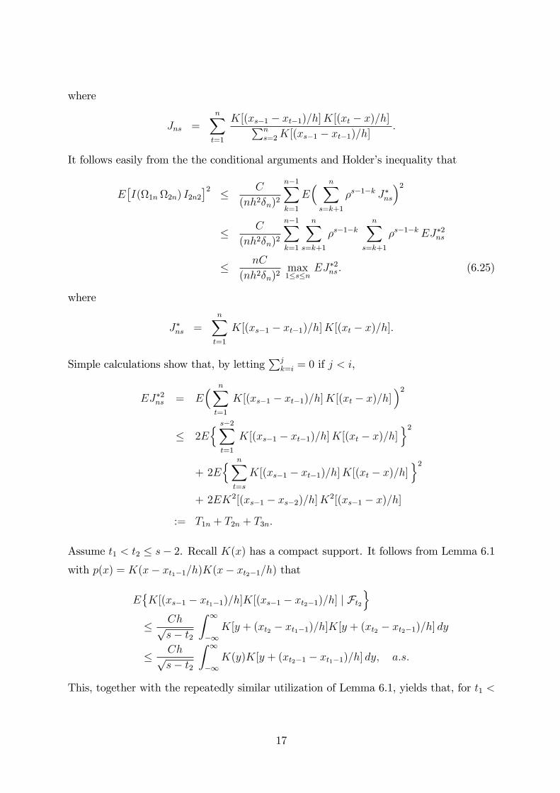
Jns =n∑t=1

K[(xs−1 − xt−1)/h]K[(xt − x)/h]∑ns=2K[(xs−1 − xt−1)/h]

.

It follows easily from the the conditional arguments and Holder’s inequality that

E[I(Ω1n Ω2n) I2n2

]2 ≤ C

(nh2δn)2

n−1∑k=1

E( n∑s=k+1

ρs−1−k J∗ns

)2≤ C

(nh2δn)2

n−1∑k=1

n∑s=k+1

ρs−1−kn∑

s=k+1

ρs−1−k EJ∗2ns

≤ nC

(nh2δn)2max1≤s≤n

EJ∗2ns . (6.25)

where

J∗ns =n∑t=1

K[(xs−1 − xt−1)/h]K[(xt − x)/h].

Simple calculations show that, by letting∑j

k=i = 0 if j < i,

EJ∗2ns = E( n∑t=1

K[(xs−1 − xt−1)/h]K[(xt − x)/h])2

≤ 2E s−2∑

t=1

K[(xs−1 − xt−1)/h]K[(xt − x)/h]2

+ 2E n∑

t=s

K[(xs−1 − xt−1)/h]K[(xt − x)/h]2

+ 2EK2[(xs−1 − xs−2)/h]K2[(xs−1 − x)/h]

:= T1n + T2n + T3n.

Assume t1 < t2 ≤ s− 2. Recall K(x) has a compact support. It follows from Lemma 6.1

with p(x) = K(x− xt1−1/h)K(x− xt2−1/h) that

EK[(xs−1 − xt1−1)/h]K[(xs−1 − xt2−1)/h] | Ft2

≤ Ch√

s− t2

∫ ∞−∞

K[y + (xt2 − xt1−1)/h]K[y + (xt2 − xt2−1)/h] dy

≤ Ch√s− t2

∫ ∞−∞

K(y)K[y + (xt2−1 − xt1−1)/h] dy, a.s.

This, together with the repeatedly similar utilization of Lemma 6.1, yields that, for t1 <

17

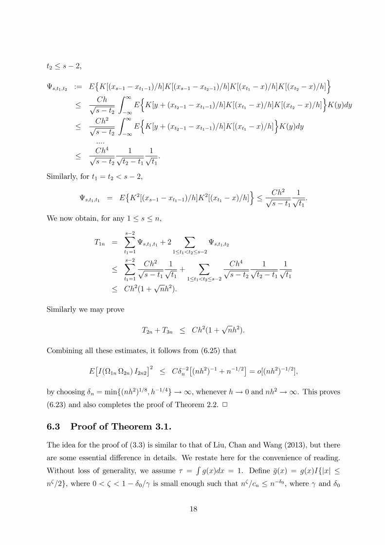
t2 ≤ s− 2,

Ψs,t1,t2 := EK[(xs−1 − xt1−1)/h]K[(xs−1 − xt2−1)/h]K[(xt1 − x)/h]K[(xt2 − x)/h]

≤ Ch√

s− t2

∫ ∞−∞

EK[y + (xt2−1 − xt1−1)/h]K[(xt1 − x)/h]K[(xt2 − x)/h]

K(y)dy

≤ Ch2√s− t2

∫ ∞−∞

EK[y + (xt2−1 − xt1−1)/h]K[(xt1 − x)/h]

K(y)dy

....

≤ Ch4√s− t2

1√t2 − t1

1√t1.

Similarly, for t1 = t2 < s− 2,

Ψs,t1,t1 = EK2[(xs−1 − xt1−1)/h]K2[(xt1 − x)/h]

≤ Ch2√

s− t11√t1.

We now obtain, for any 1 ≤ s ≤ n,

T1n =s−2∑t1=1

Ψs,t1,t1 + 2∑

1≤t1<t2≤s−2Ψs,t1,t2

≤s−2∑t1=1

Ch2√s− t1

1√t1

+∑

1≤t1<t2≤s−2

Ch4√s− t2

1√t2 − t1

1√t1

≤ Ch2(1 +√nh2).

Similarly we may prove

T2n + T3n ≤ Ch2(1 +√nh2).

Combining all these estimates, it follows from (6.25) that

E[I(Ω1n Ω2n) I2n2

]2 ≤ Cδ−2n[(nh2)−1 + n−1/2

]= o[(nh2)−1/2],

by choosing δn = min(nh2)1/8, h−1/4 → ∞, whenever h→ 0 and nh2 →∞. This proves(6.23) and also completes the proof of Theorem 2.2. 2

6.3 Proof of Theorem 3.1.

The idea for the proof of (3.3) is similar to that of Liu, Chan and Wang (2013), but there

are some essential difference in details. We restate here for the convenience of reading.

Without loss of generality, we assume τ =∫g(x)dx = 1. Define g(x) = g(x)I|x| ≤

nζ/2, where 0 < ζ < 1 − δ0/γ is small enough such that nζ/cn ≤ n−δ0 , where γ and δ0

18

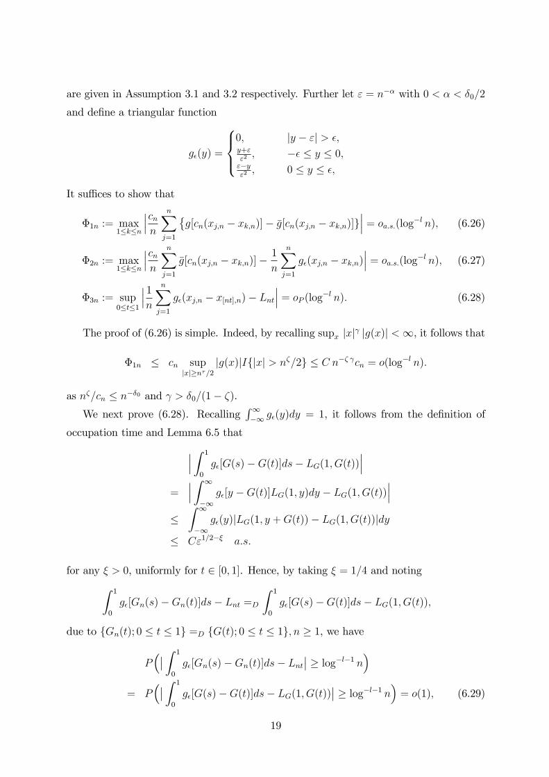
are given in Assumption 3.1 and 3.2 respectively. Further let ε = n−α with 0 < α < δ0/2

and define a triangular function

gε(y) =

0, |y − ε| > ε,y+εε2, −ε ≤ y ≤ 0,

ε−yε2, 0 ≤ y ≤ ε,

It suffi ces to show that

Φ1n := max1≤k≤n

∣∣∣cnn

n∑j=1

g[cn(xj,n − xk,n)]− g[cn(xj,n − xk,n)]

∣∣∣ = oa.s.(log−l n), (6.26)

Φ2n := max1≤k≤n

∣∣∣cnn

n∑j=1

g[cn(xj,n − xk,n)]− 1

n

n∑j=1

gε(xj,n − xk,n)∣∣∣ = oa.s.(log−l n), (6.27)

Φ3n := sup0≤t≤1

∣∣∣ 1n

n∑j=1

gε(xj,n − x[nt],n)− Lnt∣∣∣ = oP (log−l n). (6.28)

The proof of (6.26) is simple. Indeed, by recalling supx |x|γ |g(x)| <∞, it follows that

Φ1n ≤ cn sup|x|≥nτ/2

|g(x)|I|x| > nζ/2 ≤ C n−ζ γcn = o(log−l n).

as nζ/cn ≤ n−δ0 and γ > δ0/(1− ζ).

We next prove (6.28). Recalling∫∞−∞ gε(y)dy = 1, it follows from the definition of

occupation time and Lemma 6.5 that∣∣∣ ∫ 1

0

gε[G(s)−G(t)]ds− LG(1, G(t))∣∣∣

=∣∣∣ ∫ ∞−∞

gε[y −G(t)]LG(1, y)dy − LG(1, G(t))∣∣∣

≤∫ ∞−∞

gε(y)|LG(1, y +G(t))− LG(1, G(t))|dy

≤ Cε1/2−ξ a.s.

for any ξ > 0, uniformly for t ∈ [0, 1]. Hence, by taking ξ = 1/4 and noting∫ 1

0

gε[Gn(s)−Gn(t)]ds− Lnt =D

∫ 1

0

gε[G(s)−G(t)]ds− LG(1, G(t)),

due to Gn(t); 0 ≤ t ≤ 1 =D G(t); 0 ≤ t ≤ 1, n ≥ 1, we have

P(∣∣ ∫ 1

0

gε[Gn(s)−Gn(t)]ds− Lnt∣∣ ≥ log−l−1 n

)= P

(∣∣ ∫ 1

0

gε[G(s)−G(t)]ds− LG(1, G(t))∣∣ ≥ log−l−1 n

)= o(1), (6.29)

19

as n → ∞. This, together with Assumption 3.2 and the fact that |gε(y) − gε(z)| ≤ε−2|y − z|, implies that∣∣∣ 1

n

n∑j=1

gε(xj,n − x[nt],n)− Lnt∣∣∣

≤∣∣∣ ∫ 1

0

gε(x[ns],n − x[nt],n)ds−∫ 1

0

gε[Gn(s)−Gn(t)]ds∣∣∣+ 2/(εn)

+∣∣∣ ∫ 1

0

gε[Gn(s)−Gn(t)]ds− Lnt∣∣∣

= Oa.s(ε−2n−δ0) + 2/(εn) +OP (log−l−1 n)

≤ OP (n2α−δ0 + log−l−1 n) = oP (log−l n),

uniformly for t ∈ [0, 1], as α < δ0/2. This yields (6.28 ).

We finally prove (6.27), let gεn(z) be the step function which takes the value gε(mnζ/cn)

for z ∈ [mnζ/cn, (m+1)nζ/cn),m ∈ Z. It suffi ces to show that, uniformly for all 1 ≤ k ≤ n,

(letting gj(y) = g(cn(xj,n − xk,n)− y)),

∆1n(k) :=∣∣∣ 1n

n∑j=1

gε(xj,n − xk,n)− 1

n

n∑j=1

gεn(xj,n − xk,n)

∫ ∞−∞

gj(y)dy∣∣∣

= oa.s.(log−l n) (6.30)

∆2n(k) :=∣∣∣ 1n

n∑j=1

gεn(xj,n − xk,n)

∫ ∞−∞

gj(y)dy −∫ ∞−∞

1

n

n∑j=1

gε(y/cn)gj(y)dy∣∣∣

= oa.s.(log−l n), (6.31)

∆3n(k) :=∣∣∣ ∫ ∞−∞

1

n

n∑j=1

gε(y/cn)gj(y)dy − cnn

n∑j=1

g[cn(xj,n − xk,n)]∣∣∣

= oa.s.(log−l n), (6.32)

In fact, by noting that |gε(y)− gε(z)| ≤ ε−2|y − z| and

|gε n(y)− gε(z)| ≤ |gε n(y)− gε(y)|+ |gε(y)− gε(z)|

≤ Cε−2(nζ/cn + |y − z|), (6.33)

(6.30) follows from that, uniformly for all 1 ≤ j, k ≤ n,∣∣∣gε(xj,n − xk,n)− gεn(xj,n − xk,n)

∫ ∞−∞

gj(y)dy∣∣∣

≤∣∣∣gε(xj,n − xk,n)− gεn(xj,n − xk,n)

∣∣∣+ |gεn(xj,n − xk,n)|∣∣∣1− ∫ ∞

−∞gj(y)dy

∣∣∣≤ Cε−2nζ/cn + C1ε

−1 n−ζ(γ−1) = oa.s.(log−l n).

20

where we have used the fact that (recalling∫g(y)dy = 1),∣∣∣1− ∫ ∞

−∞gj(y)dy

∣∣∣ ≤ ∣∣∣ ∫ ∞−∞

g(y)I|y| > nζ/2dy∣∣∣ ≤ C n−ζ(γ−1)

due to supy |y|γ|g(y)| <∞ and γ > 1.

By the definition of gj(y) and (6.33) again, (6.31) follows from that, uniformly for all

1 ≤ j, k ≤ n,∫ ∞−∞|gεn(xj,n − xk,n)gj(y)− gε(y/cn)gj(y)|dy

≤(∫ ∞−∞

g(y)dy)(

supy

∣∣gεn(xj,n − xk,n)− gε(y/cn)∣∣ I|cn(xj,n − xk,n)− y| ≤ nζ/2

)≤ C sup

y

[ε−2(nζ/cn + |xj,n − xk,n − y/cn|) I

∣∣xj,n − xk,n − y/cn∣∣ ≤ nζ/(2cn)]

≤ Cε−2(nζ/cn) = oa.s.(log−l n).

As for (6.32), the result follows from that, by using Lemma 6.6,

∆3n(k) =∣∣∣ ∫ ∞−∞

1

n

n∑j=1

g[cn(xj,n − xk,n)− y]− g[cn(xj,n − xk,n)]

gε(y/cn)dy

∣∣∣≤ sup

tsup

|s−t|≤cnε

∣∣∣cnn

n∑j=1

g(cnxj,n + s)− g(cnxj,n + t)

∣∣∣×( 1

cn

∫ ∞−∞

gε(y/cn)dy)

= oa.s.(log−l n). (6.34)

uniformly for 1 ≤ k ≤ n.

The proof of Theorem 3.1 is complete. 2

6.4 Proof of Theorem 3.2.

To prove (3.4), we make use of Theorem 3.1. First note that K(x) satisfies Assumption

3.1 as it has a compact support. Let xk,n = xk√nφ, 1 ≤ k ≤ n, where xk satisfies Assumption

2.1 with∑∞

i=0 i|φi| <∞. As shown in Chan and Wang (2012), xk,n satisfies Assumption3.3. xk,n also satisfies Assumption 3.2. Explicitly we will show later that νj, j ∈ Zcan be redefined on a richer probability space which also contains a standard Brownian

motion W1(t) and a sequence of stochastic processes G1n(t) such that G1n(t), 0 ≤ t ≤1 =D G1(t), 0 ≤ t ≤ 1 for each n ≥ 1 and

sup0≤t≤1

|x[nt],n −G1n(t)| = o(n−δ0), a.s., (6.35)

21

for some δ0 > 0, where G1(t) = W1(t) + κ∫ t0eκ(t−s)W1(s)ds. We remark that G1(t) is a

continuous local martingale having a local time.

Due to these fact, it follows from Theorem 3.1 that

sup0≤t≤1

∣∣∣ 1√nh

n∑k=1

K[(xk − x[nt])/

√nφ]− Lnt

∣∣∣ = oP (log−l n), (6.36)

for any l > 0, h→ 0 and n1−ε0h2 →∞ where ε0 > 0 can be taken arbitrary small and

Lnt = limε→0

1

2ε

∫ 1

0

I(|G1n(s)−G1n(t)| ≤ ε)ds.

Note that, for each n ≥ 1, Lnt, 0 ≤ t ≤ 1 =D Lt, 0 ≤ t ≤ 1 due to G1n(t), 0 ≤ t ≤1 =D G1(t), 0 ≤ t ≤ 1, where Lt = limε→0

12ε

∫ 10I(|G1(s) − G1(t)| ≤ ε)ds. The result

(3.4) now follow from (6.36) and the well-know fact that P (inf0≤t≤1 Lt = 0) = 0, due to

the continuity of the process G1(s).

To end the proof of (3.4), it remains to show (6.35). In fact, the classical strong

approximation theorem implies that, on a richer probability space,

sup0≤t≤1

∣∣ [nt]∑j=1

νj −W1(nt)∣∣ = o

[n1/(2+δ)

], a.s. (6.37)

See, e.g., Csörgö and Révész (1981). Taking this result into consideration, the same

technique as in the proof of Phillips (1987) [see also Chan and Wei (1987)] yields

sup0≤t≤1

∣∣ [nt]∑j=1

λ[nt]−jνj −G∗1n(t)∣∣ = o

[n1/(2+δ)

], a.s., (6.38)

where G∗1n(t) = W1(nt) + κ∫ t0eκ(t−s)W1(ns)ds. Let G1n(t) = G∗1n(t)/

√n. It is readily

seen that G1n(t), 0 ≤ t ≤ 1 =D G1(t), 0 ≤ t ≤ 1 due to W1(nt)/√n, 0 ≤ t ≤ 1 =D

W1(t), 0 ≤ t ≤ 1. Now, by virtue of (6.7)-(6.8), the result (6.35) follows from that

sup0≤t≤1

|x[nt],n −G1n(t)| ≤ sup0≤t≤1

|a[nt] x

′[nt]√

nφ−G1n(t)|+

sup0≤t≤1 |x′′[nt] + x′′′[nt]|√nφ

≤ C√n

sup0≤t≤1

|( [nt]∑i=0

φiλ−i − φ

) [nt]∑j=1

λ[nt]−jνj|

1√n

sup0≤t≤1

∣∣ [nt]∑j=1

λ[nt]−jνj −G∗1n(t)∣∣+Oa.s.(n

−δ/2(2+δ))

= o(n−δ0), a.s.,

22

for some δ0 > 0, where we have used the fact: due to max1≤i≤n |λ−i − 1| ≤ Cn−1/2 and

max1≤k≤n |∑k

j=1 λk−jνj| = o(

√n log n), a.s., it follows from

∑∞i=0 i|φi| <∞ that

sup0≤t≤1

|( [nt]∑i=0

φiλ−i − φ

) [nt]∑j=1

λ[nt]−jνj|

≤ C max1≤k≤

√n|

k∑j=1

λk−jνj|+O(√n log n) max√

n≤k≤n|

k∑i=0

φiλ−i − φ|

≤ OP (n1/4√

log n) +O(√n log n)

(∣∣ √n∑i=0

φi(λ−i − 1)

∣∣+∞∑

i=√n

|φi|)

= O(n1/4√

log n), a.s.

We finally prove (3.5). Simple calculations show that

Vn ≤2

n

n∑t=1

(J21t + J22t), (6.39)

where

J1t =

∑ns=2

[m(xs−1)−m(xt)

]K[(xs−1 − xt)/h]∑n

s=2K[(xs−1 − xt)/h], J2t =

∑ns=2 us−1K[(xs−1 − xt)/h]∑n

s=2K[(xs−1 − xt)/h].

Assumption 2.4(a) implies that, when |xs−1 − xt| ≤M h and h is suffi ciently small,

|m(xs−1)−m(xt)| ≤ C |xs−1 − xt|β(1 + |xt|α),

uniformly on s, t. Using this fact and K has a compact support, it follows that

1

n

n∑t=1

J21t ≤C h2β

n

n∑t=1

(1 + |xt|2α) = OP (nαh2β). (6.40)

As for J2t, by recalling us =∑s

k=1 ρs−kεk, we have

1

n

n∑t=1

J22t ≤

inft=1,...,n

n∑s=1

K[(xs − xt)/h]−1 1

n

n∑t=1

J∗22t ,

where

J∗2t =

∑n−1k=1 εk

∑n−1s=k ρ

s−kK[(xs − xt)/h](∑n−1s=1 K[(xs − xt)/h]

)1/2 .

It follows from Assumption 2.2 that, for 1 ≤ t ≤ n,

E(J∗22t | x1, ..., xn) ≤

∑n−1k=1 E(ε2k | x1, ..., xn)

∑n−1s=k ρ

s−kK[(xs − xt)/h]2

∑n−1s=1 K[(xs − xt)/h]

≤ C∑n−1

k=1

∑n−1s=k ρ

s−kK2[(xs − xt)/h]∑n−1

s=k ρs−k∑n−1

s=1 K[(xs − xt)/h]

≤ C1,

23

where we have used the fact that∑∞

k=0 ρk = 1/(1− ρ) <∞. Hence 1

n

∑nt=1 J

∗22t = OP (1).

Due to this fact and (3.4), we get

1

n

n∑t=1

J22t = OP [(nh2)−1/2]. (6.41)

Combining (6.39)—(6.41), we prove (3.5) and hence complete the proof of Theorem 3.2. 2

REFERENCES

Cai, Z., Li, Q. and Park, J. Y. (2009). Functional-coeffi cient models for nonstationary

time series data. J. Econometrics 148, 101—113.

Chan, N. and Wang, Q. (2012). Uniform convergence for Nadaraya-Watson estimators

with non-stationary data. Econometric Theory, conditionally accepted.

Chan, N. H. and Wei, C. Z. (1987). Asymptotic inference for nearly nonstationary AR(1)

process. Annals of Statistics, 15, 1050-1063.

Csörgö, M. and Révész, P. (1981). Strong approximations in probability and statistics.

Probability and Mathematical Statistics. Academic Press, Inc., New York-London

Engle, R.F. and C.W.J. Granger (1987). Cointegration and Error Correction: Represen-

tation, Estimation, and Testing, Econometrica, 55, 251-276.

Hall, P.; Heyde, C. C. (1980). Martingale limit theory and its application, Probability

and Mathematical Statistics. Academic Press, Inc.

Johansen, S. (1988) . Statistical Analysis of Cointegrating Vectors, Journal of Economic

Dynamics and Control, 12, 231-54.

Linton, O.B., and E, Mammen (2008). Nonparametric Transformation to White Noise

Journal of Econometrics 141, 241-264.

Liu, W., Chan, N. and Wang, Q. (2013). Uniform approximation to local time with

applications in non-linear co-integrating regression. Preprint.

Karlsen, H. A.; Tjøstheim, D. (2001). Nonparametric estimation in null recurrent time

series. Ann. Statist. 29, 372—416.

Karlsen, H. A., Myklebust, T. and Tjøstheim, D. (2007). Nonparametric estimation in a

nonlinear cointegration model, Ann. Statist., 35, 252-299.

Park, J. Y. and P. C. B. Phillips (2001). Nonlinear regressions with integrated time

series, Econometrica, 69, 117-161.

24

Phillips, P. C. B. (1987). Towards a unified asymptotic theory for autoregression. Bio-

metrika, 74, 535-547.

Phillips, P. C. B. (1988): Regression Theory for Near-Integrated Time Series, Econo-

metrica, 56, 1021—1044.

Phillips, P.C.B. (1991). Optimal Inference in Cointegrated Systems. Econometrica,

59(2), 283-306.

Phillips, P. C. B. and J. Y. Park (1998). Nonstationary Density Estimation and Kernel

Autoregression. Cowles Foundation discuss paper No. 1181.

Phillips, P. C. B., and Durlauf, S. N. (1986): Multiple Time Series Regression With

Integrated Processes, Review of Economic Studies, 53, 473—495.

Phillips, P. C. B., and Hansen, B. E.(1990): Statistical Inference in Instrumental Variables

Regression With I(1) Processes, Review of Economic Studies, 57, 99—125.

Revuz, D. and Yor, M. (1994) Continuous Martingales and Brownian Motion. Funda-

mental Principles of Mathematical Sciences 293. Springer-Verlag

Schienle, M. (2008). Nonparametric Nonstationary Regression, Unpublished Ph.D. The-

sis, University of Mannheim.

Stock, J. H. (1987): Asymptotic Properties of Least Squares Estimators of Cointegration

Vectors, Econometrica, 55, 1035—1056.

Wang, Q. and P. C. B. Phillips (2009a). Asymptotic Theory for Local Time Density

Estimation and Nonparametric Cointegrating Regression, Econometric Theory, 25,

710-738.

Wang, Q. and P. C. B. Phillips (2009b). Structural Nonparametric Cointegrating Re-

gression, Econometrica, 77, 1901-1948.

Wang, Q. and P. C. B. Phillips (2011). Asymptotic Theory for Zero Energy Functionals

with Nonparametric Regression Applications. Econometric Theory, 27, 235-259.

Wang, Q. and Phillips, P. C. B., (2012). A specification test for nonlinear nonstationary

models. The Annals of Statistics, 40, 727-758.

Xiao, Z., O. Linton, R. J. Carroll, and E. Mammen (2003). More Effi cient Local Polyno-

mial Estimation in Nonparametric Regression with Autocorrelated Errors Journal of

the American Statistical Association 98, 980-992.

25

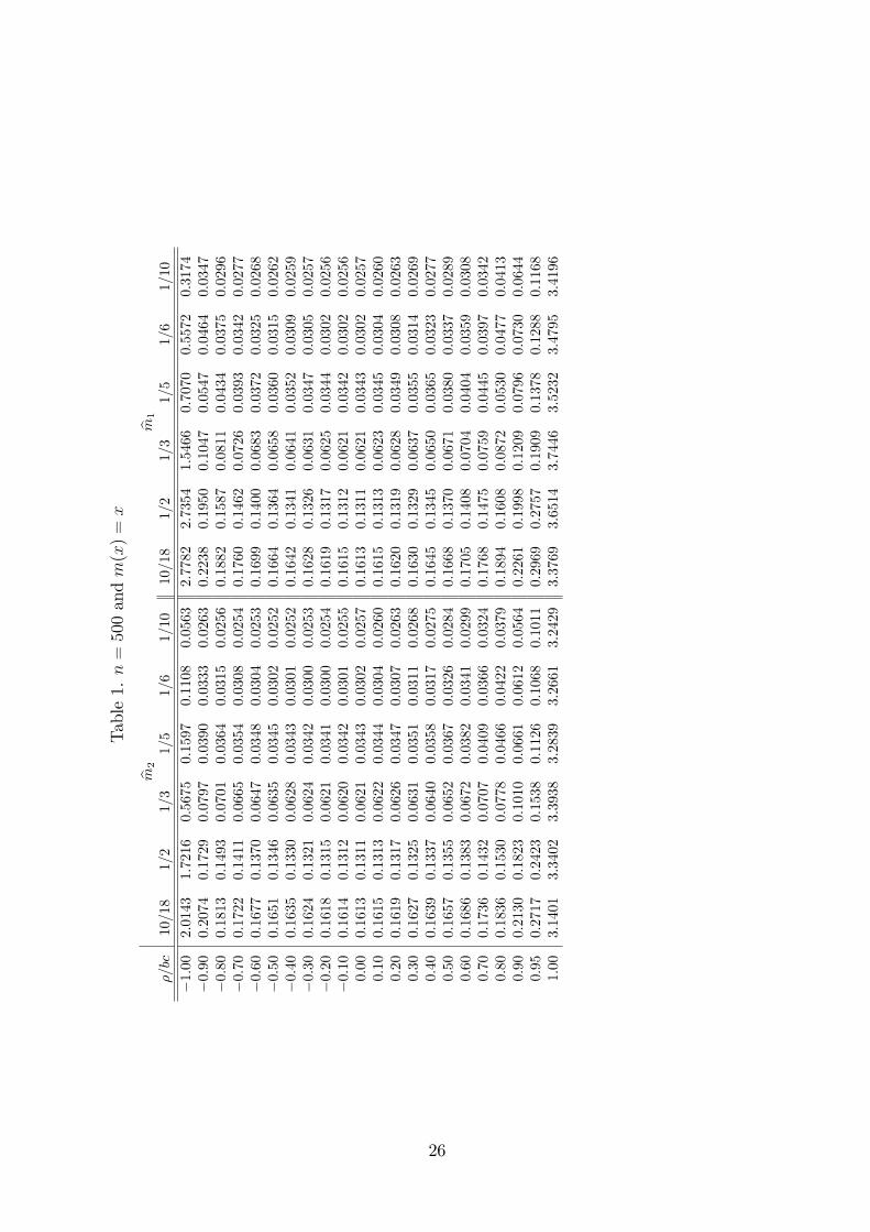
Table1.n

=50

0andm

(x)

=x

m2

m1

ρ/bc

10/18

1/2

1/3

1/5

1/6

1/10

10/18

1/2

1/3

1/5

1/6

1/10

−1.00

2.0143

1.7216

0.5675

0.1597

0.1108

0.0563

2.7782

2.7354

1.5466

0.7070

0.5572

0.3174

−0.90

0.2074

0.1729

0.0797

0.0390

0.0333

0.0263

0.2238

0.1950

0.1047

0.0547

0.0464

0.0347

−0.80

0.1813

0.1493

0.0701

0.0364

0.0315

0.0256

0.1882

0.1587

0.0811

0.0434

0.0375

0.0296

−0.70

0.1722

0.1411

0.0665

0.0354

0.0308

0.0254

0.1760

0.1462

0.0726

0.0393

0.0342

0.0277

−0.60

0.1677

0.1370

0.0647

0.0348

0.0304

0.0253

0.1699

0.1400

0.0683

0.0372

0.0325

0.0268

−0.50

0.1651

0.1346

0.0635

0.0345

0.0302

0.0252

0.1664

0.1364

0.0658

0.0360

0.0315

0.0262

−0.40

0.1635

0.1330

0.0628

0.0343

0.0301

0.0252

0.1642

0.1341

0.0641

0.0352

0.0309

0.0259

−0.30

0.1624

0.1321

0.0624

0.0342

0.0300

0.0253

0.1628

0.1326

0.0631

0.0347

0.0305

0.0257

−0.20

0.1618

0.1315

0.0621

0.0341

0.0300

0.0254

0.1619

0.1317

0.0625

0.0344

0.0302

0.0256

−0.10

0.1614

0.1312

0.0620

0.0342

0.0301

0.0255

0.1615

0.1312

0.0621

0.0342

0.0302

0.0256

0.00

0.1613

0.1311

0.0621

0.0343

0.0302

0.0257

0.1613

0.1311

0.0621

0.0343

0.0302

0.0257

0.10

0.1615

0.1313

0.0622

0.0344

0.0304

0.0260

0.1615

0.1313

0.0623

0.0345

0.0304

0.0260

0.20

0.1619

0.1317

0.0626

0.0347

0.0307

0.0263

0.1620

0.1319

0.0628

0.0349

0.0308

0.0263

0.30

0.1627

0.1325

0.0631

0.0351

0.0311

0.0268

0.1630

0.1329

0.0637

0.0355

0.0314

0.0269

0.40

0.1639

0.1337

0.0640

0.0358

0.0317

0.0275

0.1645

0.1345

0.0650

0.0365

0.0323

0.0277

0.50

0.1657

0.1355

0.0652

0.0367

0.0326

0.0284

0.1668

0.1370

0.0671

0.0380

0.0337

0.0289

0.60

0.1686

0.1383

0.0672

0.0382

0.0341

0.0299

0.1705

0.1408

0.0704

0.0404

0.0359

0.0308

0.70

0.1736

0.1432

0.0707

0.0409

0.0366

0.0324

0.1768

0.1475

0.0759

0.0445

0.0397

0.0342

0.80

0.1836

0.1530

0.0778

0.0466

0.0422

0.0379

0.1894

0.1608

0.0872

0.0530

0.0477

0.0413

0.90

0.2130

0.1823

0.1010

0.0661

0.0612

0.0564

0.2261

0.1998

0.1209

0.0796

0.0730

0.0644

0.95

0.2717

0.2423

0.1538

0.1126

0.1068

0.1011

0.2969

0.2757

0.1909

0.1378

0.1288

0.1168

1.00

3.1401

3.3402

3.3938

3.2839

3.2661

3.2429

3.3769

3.6514

3.7446

3.5232

3.4795

3.4196

26

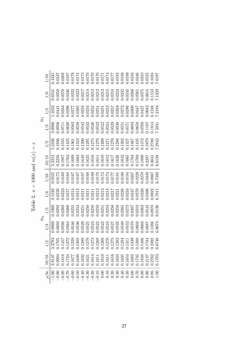
Table2.n

=10

00andm

(x)

=x

m2

m1

ρ/bc

10/18

1/2

1/3

1/5

1/6

1/10

10/18

1/2

1/3

1/5

1/6

1/10

−1.00

3.9147

3.3783

0.9869

0.1960

0.1248

0.0525

5.3312

5.3166

3.0086

1.1622

0.8541

0.4341

−0.90

0.2094

0.1705

0.0693

0.0292

0.0239

0.0175

0.2256

0.1936

0.0956

0.0441

0.0359

0.0247

−0.80

0.1818

0.1457

0.0598

0.0269

0.0223

0.0169

0.1887

0.1555

0.0711

0.0334

0.0276

0.0202

−0.70

0.1724

0.1372

0.0564

0.0260

0.0217

0.0168

0.1762

0.1425

0.0626

0.0296

0.0246

0.0187

−0.60

0.1677

0.1329

0.0546

0.0255

0.0214

0.0167

0.1699

0.1361

0.0583

0.0277

0.0232

0.0179

−0.50

0.1649

0.1305

0.0536

0.0253

0.0212

0.0167

0.1663

0.1324

0.0558

0.0265

0.0223

0.0174

−0.40

0.1632

0.1289

0.0529

0.0251

0.0211

0.0167

0.1640

0.1300

0.0542

0.0258

0.0217

0.0172

−0.30

0.1621

0.1279

0.0525

0.0250

0.0211

0.0168

0.1625

0.1285

0.0532

0.0254

0.0214

0.0170

−0.20

0.1614

0.1273

0.0523

0.0250

0.0211

0.0169

0.1616

0.1275

0.0526

0.0252

0.0212

0.0170

−0.10

0.1611

0.1269

0.0522

0.0250

0.0212

0.0170

0.1611

0.1270

0.0523

0.0251

0.0212

0.0170

0.00

0.1610

0.1269

0.0522

0.0251

0.0213

0.0172

0.1610

0.1269

0.0522

0.0251

0.0213

0.0171

0.10

0.1611

0.1270

0.0524

0.0253

0.0214

0.0174

0.1612

0.1271

0.0524

0.0253

0.0215

0.0174

0.20

0.1616

0.1275

0.0527

0.0256

0.0217

0.0177

0.1617

0.1276

0.0529

0.0257

0.0218

0.0177

0.30

0.1623

0.1282

0.0532

0.0259

0.0221

0.0181

0.1626

0.1286

0.0538

0.0263

0.0224

0.0182

0.40

0.1635

0.1294

0.0540

0.0265

0.0226

0.0186

0.1642

0.1302

0.0551

0.0272

0.0232

0.0189

0.50

0.1654

0.1311

0.0552

0.0273

0.0234

0.0194

0.1665

0.1327

0.0571

0.0286

0.0245

0.0199

0.60

0.1683

0.1339

0.0570

0.0287

0.0247

0.0207

0.1703

0.1367

0.0603

0.0309

0.0266

0.0216

0.70

0.1735

0.1388

0.0602

0.0310

0.0270

0.0229

0.1768

0.1435

0.0658

0.0347

0.0301

0.0246

0.80

0.1838

0.1486

0.0668

0.0363

0.0320

0.0278

0.1899

0.1572

0.0769

0.0427

0.0375

0.0310

0.90

0.2147

0.1784

0.0887

0.0543

0.0496

0.0449

0.2287

0.1979

0.1107

0.0682

0.0615

0.0525

0.95

0.2762

0.2392

0.1386

0.0978

0.0922

0.0867

0.3041

0.2780

0.1814

0.1248

0.1153

0.1024

1.00

6.1783

6.6740

6.9673

6.8136

6.7811

6.7500

6.6138

7.2842

7.5941

7.2184

7.1329

7.0197

27

Table3.Eρ,

m(x

)=

sin(x

)

n=1000

n=500

ρ/bc

10/18

1/2

1/3

1/5

1/6

1/10

10/18

1/2

1/3

1/5

1/6

1/10

−1.00

-0.4587

-0.5555

-0.8031

-0.9151

-0.9330

-0.9600

-0.4627

-0.5496

-0.7803

-0.8962

-0.9158

-0.9464

−0.90

-0.4148

-0.5021

-0.7239

-0.8239

-0.8393

-0.8601

-0.4215

-0.5002

-0.7071

-0.8083

-0.8247

-0.8475

−0.80

-0.3704

-0.4478

-0.6451

-0.7330

-0.7462

-0.7616

-0.3773

-0.4474

-0.6310

-0.7194

-0.7331

-0.7492

−0.70

-0.3259

-0.3934

-0.5661

-0.6424

-0.6534

-0.6644

-0.3326

-0.3940

-0.5547

-0.6309

-0.6421

-0.6529

−0.60

-0.2814

-0.3391

-0.4871

-0.5521

-0.5612

-0.5686

-0.2877

-0.3403

-0.4783

-0.5429

-0.5519

-0.5584

−0.50

-0.2368

-0.2849

-0.4082

-0.4622

-0.4695

-0.4740

-0.2427

-0.2867

-0.4019

-0.4554

-0.4624

-0.4657

−0.40

-0.1922

-0.2307

-0.3295

-0.3726

-0.3783

-0.3804

-0.1977

-0.2330

-0.3257

-0.3683

-0.3736

-0.3743

−0.30

-0.1476

-0.1765

-0.2508

-0.2833

-0.2874

-0.2876

-0.1527

-0.1792

-0.2496

-0.2817

-0.2854

-0.2842

−0.20

-0.1030

-0.1223

-0.1721

-0.1942

-0.1968

-0.1955

-0.1078

-0.1255

-0.1735

-0.1953

-0.1975

-0.1949

−0.10

-0.0583

-0.0681

-0.0935

-0.1052

-0.1064

-0.1038

-0.0628

-0.0718

-0.0974

-0.1091

-0.1099

-0.1062

0.00

-0.0137

-0.0138

-0.0149

-0.0163

-0.0161

-0.0124

-0.0179

-0.0181

-0.0213

-0.0230

-0.0225

-0.0179

0.10

0.0310

0.0405

0.0637

0.0726

0.0741

0.0789

0.0270

0.0356

0.0549

0.0632

0.0649

0.0702

0.20

0.0756

0.0948

0.1424

0.1616

0.1645

0.1702

0.0720

0.0893

0.1311

0.1494

0.1524

0.1585

0.30

0.1204

0.1492

0.2212

0.2507

0.2550

0.2618

0.1169

0.1432

0.2075

0.2358

0.2401

0.2471

0.40

0.1652

0.2037

0.3000

0.3400

0.3457

0.3538

0.1619

0.1971

0.2841

0.3225

0.3282

0.3363

0.50

0.2100

0.2583

0.3791

0.4296

0.4368

0.4464

0.2070

0.2511

0.3608

0.4095

0.4167

0.4263

0.60

0.2550

0.3131

0.4583

0.5196

0.5284

0.5398

0.2521

0.3052

0.4378

0.4971

0.5059

0.5173

0.70

0.3003

0.3683

0.5380

0.6101

0.6206

0.6343

0.2974

0.3596

0.5152

0.5853

0.5959

0.6098

0.80

0.3461

0.4241

0.6183

0.7015

0.7137

0.7303

0.3432

0.4144

0.5932

0.6745

0.6871

0.7043

0.90

0.3930

0.4811

0.7003

0.7946

0.8088

0.8287

0.3902

0.4702

0.6730

0.7659

0.7807

0.8017

0.95

0.4174

0.5109

0.7433

0.8430

0.8581

0.8799

0.4153

0.4996

0.7147

0.8135

0.8293

0.8523

1.00

0.4466

0.5462

0.7903

0.8935

0.9093

0.9324

0.4399

0.5296

0.7567

0.8614

0.8781

0.9033

28

Table4.

stdc(ρ),m

(x)

=si

n(x

)

n=1000

n=500

ρ/bc

10/18

1/2

1/3

1/5

1/6

1/10

10/18

1/2

1/3

1/5

1/6

1/10

−1.00

0.0805

0.0816

0.0557

0.0283

0.0229

0.0145

0.0829

0.0835

0.0611

0.0344

0.0288

0.0197

−0.90

0.0706

0.0704

0.0466

0.0265

0.0230

0.0187

0.0756

0.0733

0.0512

0.0333

0.0302

0.0261

−0.80

0.0635

0.0634

0.0429

0.0269

0.0245

0.0220

0.0704

0.0672

0.0481

0.0346

0.0327

0.0307

−0.70

0.0568

0.0568

0.0399

0.0276

0.0261

0.0247

0.0650

0.0617

0.0463

0.0364

0.0353

0.0346

−0.60

0.0505

0.0506

0.0374

0.0284

0.0274

0.0267

0.0599

0.0568

0.0453

0.0382

0.0377

0.0378

−0.50

0.0450

0.0450

0.0353

0.0291

0.0285

0.0283

0.0554

0.0527

0.0447

0.0400

0.0398

0.0402

−0.40

0.0403

0.0402

0.0336

0.0298

0.0295

0.0295

0.0518

0.0495

0.0444

0.0417

0.0417

0.0422

−0.30

0.0366

0.0363

0.0325

0.0305

0.0304

0.0305

0.0491

0.0473

0.0445

0.0432

0.0433

0.0437

−0.20

0.0342

0.0336

0.0320

0.0311

0.0311

0.0312

0.0476

0.0461

0.0450

0.0446

0.0446

0.0450

−0.10

0.0331

0.0323

0.0321

0.0318

0.0318

0.0318

0.0470

0.0459

0.0457

0.0457

0.0457

0.0459

0.00

0.0334

0.0326

0.0327

0.0325

0.0325

0.0323

0.0474

0.0466

0.0467

0.0467

0.0467

0.0467

0.10

0.0351

0.0345

0.0339

0.0333

0.0331

0.0328

0.0488

0.0481

0.0479

0.0475

0.0474

0.0472

0.20

0.0381

0.0376

0.0356

0.0340

0.0337

0.0332

0.0510

0.0504

0.0493

0.0481

0.0479

0.0476

0.30

0.0419

0.0417

0.0376

0.0346

0.0341

0.0335

0.0540

0.0534

0.0508

0.0486

0.0482

0.0477

0.40

0.0466

0.0466

0.0398

0.0351

0.0344

0.0336

0.0577

0.0569

0.0525

0.0488

0.0482

0.0476

0.50

0.0517

0.0519

0.0423

0.0354

0.0344

0.0334

0.0619

0.0609

0.0543

0.0488

0.0480

0.0472

0.60

0.0573

0.0575

0.0448

0.0354

0.0341

0.0328

0.0666

0.0654

0.0561

0.0485

0.0474

0.0463

0.70

0.0633

0.0635

0.0472

0.0350

0.0333

0.0316

0.0718

0.0701

0.0580

0.0479

0.0464

0.0449

0.80

0.0697

0.0697

0.0498

0.0343

0.0322

0.0298

0.0777

0.0753

0.0599

0.0469

0.0449

0.0426

0.90

0.0767

0.0765

0.0526

0.0337

0.0309

0.0274

0.0844

0.0820

0.0618

0.0454

0.0427

0.0395

0.95

0.0803

0.0800

0.0544

0.0339

0.0307

0.0264

0.0877

0.0863

0.0628

0.0448

0.0417

0.0377

1.00

0.0869

0.0860

0.0572

0.0347

0.0310

0.0253

0.0942

0.0929

0.0668

0.0461

0.0427

0.0377

29

Figure 1. Shows the QQ plot of the standardized estimator m2

30