non-linear reasoning for invariant synthesiszkincaid/pub/popl18a.pdf · 54 non-linear reasoning for...
TRANSCRIPT
54
Non-linear Reasoning for Invariant Synthesis
ZACHARY KINCAID, Princeton University, USA
JOHN CYPHERT and JASON BRECK, University of Wisconsin, USA
THOMAS REPS, University of Wisconsin, USA and GrammaTech, Inc., USA
Automatic generation of non-linear loop invariants is a long-standing challenge in program analysis, with
many applications. For instance, reasoning about exponentials provides a way to find invariants of digital-filter
programs, and reasoning about polynomials and/or logarithms is needed for establishing invariants that
describe the time or memory usage of many well-known algorithms. An appealing approach to this challenge
is to exploit the powerful recurrence-solving techniques that have been developed in the field of computer
algebra, which can compute exact characterizations of non-linear repetitive behavior. However, there is a gap
between the capabilities of recurrence solvers and the needs of program analysis: (1) loop bodies are not merely
systems of recurrence relations—they may contain conditional branches, nested loops, non-deterministic
assignments, etc., and (2) a client program analyzer must be able to reason about the closed-form solutions
produced by a recurrence solver (e.g., to prove assertions).
This paper presents a method for generating non-linear invariants of general loops based on analyzing
recurrence relations. The key components are an abstract domain for reasoning about non-linear arithmetic, a
semantics-based method for extracting recurrence relations from loop bodies, and a recurrence solver that
avoids closed forms that involve complex or irrational numbers. Our technique has been implemented in a
program analyzer that can analyze general loops and mutually recursive procedures. Our experiments show
that our technique shows promise for non-linear assertion-checking and resource-bound generation.
CCS Concepts: • Theory of computation → Program analysis; • Software and its engineering →
Automated static analysis;
Additional Key Words and Phrases: Invariant generation, Recurrence relation, Operational calculus
ACM Reference Format:Zachary Kincaid, John Cyphert, Jason Breck, and Thomas Reps. 2018. Non-linear Reasoning for Invariant
Synthesis . Proc. ACM Program. Lang. 2, POPL, Article 54 (January 2018), 33 pages. https://doi.org/10.1145/
3158142
1 INTRODUCTIONRecurrence equations have a long history, and variety of techniques for solving them are known. A
natural question is to ask how these techniques can be put to work for invariant generation.
One line of work in this direction focuses on computing very accurate information about a syn-
tactically restricted class of loops. For example, Rodríguez-Carbonell and Kapur [2004] and Kovács
[2008] use recurrence solving to compute all invariant polynomial equations of two (different)
classes of loops. Neither technique can compute any invariants for loops that have (for example)
nondeterministic assignments or nested loops.
Authors’ addresses: Zachary Kincaid, [email protected], Princeton University, USA; John Cyphert, jcyphert@
wisc.edu; Jason Breck, [email protected], University of Wisconsin, USA; Thomas Reps, [email protected], University of
Wisconsin, USA, GrammaTech, Inc. USA.
Permission to make digital or hard copies of all or part of this work for personal or classroom use is granted without fee
provided that copies are not made or distributed for profit or commercial advantage and that copies bear this notice and
the full citation on the first page. Copyrights for components of this work owned by others than ACM must be honored.
Abstracting with credit is permitted. To copy otherwise, or republish, to post on servers or to redistribute to lists, requires
prior specific permission and/or a fee. Request permissions from [email protected].
© 2018 Association for Computing Machinery.
2475-1421/2018/1-ART54
https://doi.org/10.1145/3158142
Proceedings of the ACM on Programming Languages, Vol. 2, No. POPL, Article 54. Publication date: January 2018.
54:2 Zachary Kincaid, John Cyphert, Jason Breck, and Thomas Reps
Compositional recurrence analysis (CRA) [Farzan and Kincaid 2015] is another line of work, which
focuses on over-approximate analysis of general loops rather than precise analysis of syntactically
restricted loops. Recent work [Kincaid et al. 2017] extends the generality of CRA even further,
showing how the approach can be applied to recursive procedures as well as loops. The key idea
that makes CRA so broadly applicable is that it represents loop behavior using logical formulas, and
uses semantics-based techniques to find implied recurrence relations. However, CRA’s ability to
reason about non-linear behavior is limited by the fact that it uses SMT solving, linear algebra, and
polyhedral techniques to extract recurrences from loop bodies, and polynomial summation to solve
them. In particular, CRA is only capable of extracting recurrence relations that can be expressed
in linear integer arithmetic and that have polynomial closed forms—effectively exploiting only a
fraction of what recurrence solvers (e.g., the ones used in [Kovács 2008; Rodríguez-Carbonell and
Kapur 2004]) are capable of.
In this paper, we present extensions to the numerical-reasoning techniques underlying CRA, and
demonstrate that these extensions enable CRA to establish many non-linear numerical invariants.
The contributions of the paper are three-fold:
• We present the wedge abstract domain, a numerical abstract domain capable of reasoning
about non-linear arithmetic. Just as convex polyhedra represent properties in the conjunctive
fragment of linear arithmetic, wedges represent properties in the conjunctive fragment of
non-linear arithmetic (including polynomials, exponentials, and logarithms). The deductive
power of wedges is due to polyhedral and Gröbner-basis techniques, congruence closure, and
simple inference rules for non-linear functions. The key operation supported by the domain
is symbolic abstraction [Reps et al. 2004; Thakur and Reps 2012], which, given an arbitrary
non-linear formula φ, computes a wedge that over-approximates φ. (See §4.)• We present a semantics-based algorithm for extracting recurrence relations that are entailed
by a loop-body formula. The algorithm is based on first over-approximating the loop body
by a wedge, and then using techniques from linear algebra to extract recurrences from the
wedge. The algorithm can extract recurrences involving non-linear arithmetic and inter-
dependent program variables; the class of recurrences that can be extracted by this algorithm
corresponds to C-finite sequences [Kauers and Paule 2011, §4.2]. (See §5.)
• We present an algorithm, OCRS, that is able to solve these recurrences, and find closed-
form solutions that include polynomials, exponentials, and logarithms. OCRS is based on an
automated and enhanced form of the discrete operational calculus of Berg [1967]. Classically,
the closed forms of C-finite sequences involve algebraic irrational or algebraic complex
numbers,1but OCRS avoids non-rational numbers by using what we call implicitly interpreted
functions. Each implicitly interpreted function is associated with a term in the logic of OCRS
that exactly characterizes the function, but outside of the recurrence solver (and in particular,
within the wedge domain) an implicitly interpreted function is treated as an uninterpreted
function symbol. (See §6.)
Our approach builds upon the recent work of Kincaid et al. [2017], which extended CRA so that it
can analyze recursive programs using essentially the same approach that it uses to handle loops.
Organization. §2 illustrates the main features of our method via a series of examples. §3 presents
relevant background material. §4 presents the wedge abstract domain. §5 describes the method used
in our system for extracting a recurrence relation from a wedge. §6 presents OCRS. §7 presents
experimental results. §8 discusses related work.
1An algebraic number is a complex number that is a root of a non-zero univariate polynomial with rational coefficients.
Henceforth, we shorten “algebraic irrational” and “algebraic complex” to “irrational” and “complex,” respectively.
Proceedings of the ACM on Programming Languages, Vol. 2, No. POPL, Article 54. Publication date: January 2018.

Non-linear Reasoning for Invariant Synthesis 54:3
int ticks = 0;for(int a = 0; a < N; a++)
for(int b = 0; b < N; b++)for(int c = 0; c < N; c++)
ticks++;
(a)
int pos = 1, steps = 0, found = 0;while(pos < array_size) {
steps += 1;if (array[pos] == val) {
found = 1;break;
}if (array[pos] < val) {
pos = 2 * pos;} else {
pos = 2 * pos + 1;}
}(b)
int temp, x = -1, y = 0;for(int n = 0; n < 1; n++) {
temp = x; x = y; y = -temp;}if (y == 1) goto errorlabel;
(c)
int fib(int n, int high) {int f1 = 1, f2 = 0, temp = 0;if (high) {
while(n > 0) {f1 = f1 + f2;f2 = f1 - f2;n--;
}} else {
while(n > 0) {temp = f2;f2 = f1;f1 = f2 + temp;n--;
}}return f1;
}void main() {
int n1, n2, obs1, obs2, high1, high2;assume(n1 == n2);// Note: high1 might not equal high2obs1 = fib(n1, high1);obs2 = fib(n2, high2);assert(obs1 == obs2);
}(d)
Fig. 1. Four examples: (a) cubic-time loop nest; (b) binary search; (c) rotation in the x, y plane; (d) absence ofinformation flow.
2 OVERVIEW AND PROBLEM STATEMENTOur system follows in the tradition of CRA [Farzan and Kincaid 2015] and ICRA [Kincaid et al.
2017] in how it combines symbolic analysis and abstract interpretation:
• It uses an abstract domain of transition formulas, and thus models non-looping program
behavior precisely.
• It conservatively explores all behaviors of a loop by over-approximating the transitive closure
of the loop body: a formula for the loop body is converted into a system of recurrences, which
are then solved to create a transition formula that summarizes the overall action of the loop.
For brevity, we refer to the actions performed to analyze a loop as the star operator.This section illustrates at a high level the main features of the star operator, focusing on how the
system reasons about non-linear relationships, such as polynomials, exponentials, and logarithms.
We present two examples of running-time analysis, along with two other examples, one analyzing
a rotation, and one demonstrating information-flow analysis.
Example 2.1. Consider the loop nest shown in Fig. 1(a), which runs in cubic time. CRA analyzes
the loop nest “bottom-up”, starting from themost deeply nested loop andmoving outwards, applying
the star operator at each nesting level. Nested loops lead to a design constraint in the program
analyzer: the star operator must be able to reason about its own output.
Proceedings of the ACM on Programming Languages, Vol. 2, No. POPL, Article 54. Publication date: January 2018.

54:4 Zachary Kincaid, John Cyphert, Jason Breck, and Thomas Reps
Nesting
Level Recurrence Solution
3 c[k+1] = c[k] + 1 ∧ ticks[k+1] = ticks[k] + 1 c[k] = c[0] + k ∧ ticks[k] = ticks[0] + k2 b[k+1] = b[k] + 1 ∧ ticks[k+1] = ticks[k] + N b[k] = b[0] + k ∧ ticks[k] = ticks[0] + N ∗ k1 a[k+1] = a[k] + 1 ∧ ticks[k+1] = ticks[k] + N ∗ N a[k] = a[0] + k ∧ ticks[k] = ticks[0] + N ∗ N ∗ k
Fig. 2. Recurrences created for the nested loops in Fig. 1(a).
Fig. 2 shows the recurrences created for the program in Fig. 1(a). We use, e.g., c[k] to denote the
value of variable c at the beginning of iteration k of the innermost loop (at nesting-level 3). As
shown in Fig. 2, the body of the innermost loop can be described by a linear recurrence, and the
solution is also linear. Using the solution to that recurrence, along with the fact that the inner loop
iterates N times, we obtain a linear recurrence for the loop at nesting-level 2. However, the solution
to this recurrence is non-linear: it involves the term N ∗ k . Consequently, the body of the outer loop
(at nesting-level 1) has the following non-linear transition formula:
∃k .ticks′ = ticks + N ∗ k ∧ k ≤ N ∧ k ≥ N ∧ a′ = a + 1,
which cannot be analyzed directly using many of the classical tools of program analysis, such as
Satisfiability Modulo Theories (SMT) solvers and the abstract domain of polyhedra. Thus, although
each iteration of the outermost loop increases the value of ticks by N∗N, the recurrence-extractiontechnique of Farzan and Kincaid [2015] is unable to find the relevant recurrence. This paper presents
an extension of CRA that is able to handle polynomial recurrences such as this one, and is therefore
able to prove that the above triply nested loop increases the value of ticks by exactly N ∗ N ∗ N.
To obtain tight bounds on the running time of other programs, logarithms are required. Moreover,
loop bodies can contain branching code—and thus different paths through the loop body may be
taken on different iterations.
Example 2.2. Consider the loop shown in Fig. 1(b), which performs a binary search over a
complete binary tree that is stored in an array. Our analysis establishes that the running time of this
loop is logarithmic in array_size by first constructing a recurrence saying that, on each iteration,
steps is incremented by 1 and pos (at least) doubles:
steps[k+1] = steps[k] + 1 ∧ pos[k+1] ≥ 2pos[k].
Extraction is a nontrivial operation because the inner loop contains branching code. Moreover, the
exact behavior of the variable pos cannot be described by a recurrence equation. Instead, we must
approximate the behavior of pos by a recurrence inequation.Next, the recurrence solver finds the solution to this recurrence:
steps[k] = steps[0] + k ∧ pos[k] ≥ 2kpos[0],
and this result, in combination with the initial conditions of the loop, establishes that whenever
control reaches the head of the loop, we have pos ≥ 2steps
. The solver also establishes that, upon
exit from the loop, pos < 2(array_size), because otherwise the loop would have exited earlier.
We conclude that steps < 1 + loд2 (array_size), if array_size > 0, and steps = 0 otherwise.
This example shows that the analysis of a logarithmic-time algorithm sometimes requires finding
exponential solutions to recurrences.
Some programs have non-linear relationships that cannot be expressed using polynomials,
exponentials, and logarithms of integers.
Example 2.3. Consider the loop shown in Fig. 1(c). One iteration of the loop performs a 90-degree
clockwise rotation of the point (x, y) about the origin. Because of the mutual dependence between
x and y, we extract a matrix recurrence for this loop. Below, we show the matrix recurrence (on the
Proceedings of the ACM on Programming Languages, Vol. 2, No. POPL, Article 54. Publication date: January 2018.

Non-linear Reasoning for Invariant Synthesis 54:5
left) and the solution to that recurrence that would be obtained by a typical off-the-shelf recurrence
solver (on the right, with i being the imaginary unit).[x[k+1]
y[k+1]
]=
[0 1
−1 0
] [x[k]
y[k]
] [x[k]
y[k]
]=
[1
2((−i )k + ik ) i
2((−i )k − ik )
− i2((−i )k − ik ) 1
2((−i )k + ik )
] [x[0]
y[0]
]
Complex exponentiation concisely represents the rotation performed by this loop, but the use of
complex numbers creates a problem for the later steps of our analysis, as demonstrated below.
Suppose that we want to know whether errorlabel is reachable. We answer that question
by using an SMT solver to check the satisfiability of the transition formula from program entry
to errorlabel. Upon entry to the loop, n is initialized to 0 and the loop condition is “n < 1”, so
the loop will always execute exactly once. Thus, the value of y at the end of the loop is y[1] =− i
2((−i )1 − i1)x[0] + 1
2((−i )1 − i1)y[0] = −i ∗ i , and the relevant part of the formula for y is:
y′ = 1 ∧ y′ = −i ∗ i . (1)
If i is interpreted as the imaginary unit, then Eqn. (1) is satisfiable, which gives us the answer we
expect: errorlabel is reachable. However, we would like to be able to use an off-the-shelf SMT
solver that does not support complex numbers. Unfortunately, it is not sound to interpret Eqn. (1)
in real arithmetic with i as a symbolic constant. In real arithmetic, we know that for all a, a ∗ a ≥ 0,
and thus y′ = −i ∗ i ≤ 0, which is inconsistent with y′ = 1; thus, Eqn. (1) is unsatisfiable, which
falsely suggests that errorlabel is unreachable.
To avoid problems of this kind, we developed a recurrence solver (described in §6) that is able
to solve recurrences like the one in this example, and communicate the solutions to the rest
of our analyzer without the use of complex numbers. As a principled way to handle the issue
of communication, the paper introduces implicitly interpreted functions (IIFs) (§6.4). An IIF is a
representation of the solution to a recurrence that would otherwise need to be expressed using
complex or irrational numbers. Inside the recurrence solver, each IIF is associated with a term in
the logic of the recurrence solver, which represents an exact representation of the function (and
the recurrence solver is able to manipulate this exact representation). Outside the recurrence
solver—e.g., in the wedge domain—an IIF is treated as an uninterpreted function.
The following example illustrates that IIFs retain enough information to prove some sophisticated
program properties.
Example 2.4. Consider the program shown in Fig. 1(d), which illustrates how our analyzer is able
to establish the absence of information flow (i.e., “non-interference”), using the self-composition
technique of Barthe et al. [2004]. For procedure fib, we will assume that variable n is a low-securityinput, high is a high-security input, and the return value of fib is a low-security output. The
information-flow property that we wish to establish is that fib’s return value is unaffected by the
value passed in for high.Secure information flow is not a safety property:
2a safety property can be refuted by observing
a finite trace of a program, whereas to refute secure information flow, one has to observe two finite
traces. Barthe et al. show that secure information flow for a program P can be encoded as a safety
property of a more complicated program that consists of P followed by P ′—a second copy of Pwith its variables suitably renamed. By this means, secure information flow can be reduced to an
assertion-checking problem in the program P ; P ′. They call this technique self composition.In the program above, the self-composition technique is captured by procedure main, which uses
two calls to fib rather than two copies of fib. In main, the statement assume(n1 == n2) ensures
that the low-security inputs to the two calls on fib are arbitrary, but equal. The absence of anyconstraint on high1 and high2 means that they may have different values in the two calls to fib.
2Technically, we are referring to the so-called “termination-insensitive” secure-information-flow problem.
Proceedings of the ACM on Programming Languages, Vol. 2, No. POPL, Article 54. Publication date: January 2018.

54:6 Zachary Kincaid, John Cyphert, Jason Breck, and Thomas Reps
The goal is to prove the assertion on the last line of main, which claims that the low-security outputs
obs1 and obs2 are equal, and hence unaffected by any difference in the values of high-security
inputs high1 and high2.To convince yourself that the assertion does indeed hold, observe that the two while loops in
fib both compute the nth Fibonacci number, albeit in slightly different ways. Thus, because the
values of n1 and n2 are equal, obs1 and obs2 will be equal—even though high1 and high2 might
differ, which would cause different while loops to be executed during the two calls on fib.The challenge in analyzing this example is that the return value of fib is a complicated function
of its inputs. Classically, this function would be represented using irrational numbers: the return
value of fib(n, high) is 1√5
(( 1+√5
2)n − ( 1+
√5
2)n). As in the previous example (Ex. 2.3), we avoid
manipulation of non-rational numbers using IIFs.
In the program shown above, the analyzer summarizes the behaviors of the two while loops in
fib using two IIFs. The two IIFs are associated with equal terms in the logic of the recurrence solver.
Consequently, the wedge domain is able to prove the assertion because it sees it as a comparison of
two identical uninterpreted functions.
Problem Statement. The foregoing examples illustrate several challenges that our work addresses:
(1) The star operator takes as input a logical representation of the body of loop. The loop body
formula typically contains disjunctions, existentially quantified variables, and inequations,
and so cannot be directly interpreted as a recurrence relation. Therefore, we need an automatic
method for extracting recurrences that lie within the input language of our recurrence solver.
In general, these recurrences may include non-linear relationships.
(2) Once we have a recurrence relation, we need to solve it. In general, an extracted recurrence
may contain polynomial and exponential terms, and program variables may mutually depend
on one another. We need to be able to compute a closed form that can be represented in the
base logic of the program analyzer (see §6.3).
The analysis method presented in the paper addresses these challenges by the following means:
• Challenge (1) is addressed via a new abstract domain, called the wedge domain (§4), which
encodes non-linear relationships by extending the abstract domain of polyhedra with new
dimensions that represent non-linear terms. §5 presents an algorithm that uses the wedge
abstract domain to extract recurrence relations from a loop body formula.
• Challenge (2) is addressed via a new recurrence solver that we developed, based on the
discrete operational calculus of Berg [1967]. (See §6.)The balancing act in our work is that there is a mutual dependence between the wedge domain
and the recurrence solver: each places constraints on the other. In addressing challenges (1) and
(2), we faced a situation that often comes up in system building, namely, it is not always possible
to use an existing component as just a black box. Although methods for solving recurrences are
known (see §8 for references and a discussion), the closed forms computed by these methods may
involve irrational and complex numbers, which are not permitted in the base logic of our program
analyzer. The desire to have IIFs for reasoning outside the recurrence solver required us to have
some control over what goes on inside the recurrence solver, to identify—and return as part of the
answer—terms that define IIFs.
3 BACKGROUND3.1 Linear Real ArithmeticFix a set of variables z1, ..., zn . A linear term is an expression of the form a1z1+· · ·+anzn+b, whereeach ai ∈ Q and b ∈ Q. We will typically write such a term as az + b, where a = [a1, ...,an] and
Proceedings of the ACM on Programming Languages, Vol. 2, No. POPL, Article 54. Publication date: January 2018.

Non-linear Reasoning for Invariant Synthesis 54:7
z = [z1, ..., zn]tare vectors containing the term’s rational coefficients and variables, respectively. A
linear inequality is of the form az ≥ b. A system of linear inequalities a1z ≥ b1∧· · ·∧amz ≥ bm can
be written succinctly asAz ≥ b, whereA is a matrix whose rows are a1, ..., am , and b = [b1, ...,bm]t.
The set of points z such that Az ≥ b is a (convex) polyhedron.
3.2 (Non)linear Real Arithmetic with Uninterpreted FunctionsLet Σ = ⟨F , ar⟩ be a functional first-order vocabulary, consisting of a set of function symbols F and
a function ar : F → N associating each function symbol with an arity. We define the syntax of a
logical language that extends linear real arithmetic with the vocabulary Σ as follows:
s, t ∈ Term(Σ) ::=a ∈ Q | v ∈ Var | a × t | s + t | f(t1, ..., tar(f) )
ϕ,ψ ∈ Formula(Σ) ::= t ≥ 0 | t > 0 | ϕ ∧ψ | ϕ ∨ψ | ∃v .ϕ
A term of the form a, s + t , or a × t is called linear (with the rest called non-linear). We assume
that Σ includes a vocabulary ΣN of designated function symbols that represent multiplication,
exponentiation, logarithm, modulus, and floor, which we will write using standard notation:
Term(ΣN ) ::= ... | s × t | st | logs (t ) | s mod t | ⌊t⌋
We will make use of two different semantics for this logic. A linear structure L consists of an
interpretation of each function symbol f ∈ Σ as a function fL : Rar(f ) → R; the semantics of
numerals, addition, and numeral multiplication are the usual ones. We write L |=L ϕ to denote
that L is a linear structure that satisfies the sentence ϕ; write ϕ |=L ψ if every linear structure that
satisfies the sentence ϕ also satisfies the sentence ψ ; and write ϕ ≡L ψ if ϕ |=L ψ and ψ |=L ϕ. Anon-linear structure N is a linear structure that interprets the designated function symbols in
ΣN with their usual interpretation on their domain of definition (i.e., ×N is multiplication, logN2is
base-2 logarithm for positive arguments and arbitrary for non-positive arguments, etc). We use |=Nand ≡N to denote the non-linear analogues of |=L and ≡L . Obviously, ϕ |=L ψ implies that ϕ |=N ψ ,but the reverse does not hold. Note that membership of a pair of formulas in the relation |=L is
decidable, but |=N is not.
We are particularly interested in formulas that represent transition relations of some frag-
ment of a program. Formally, we suppose that Σ is a vocabulary that contains a designated set
PVar = {x1, ..., xn } of constant symbols and also a disjoint set PVar′ = {x′
1, ..., x′n } of primed
copies, representing the values of program variables before and after a transition. A formula ϕ’sconcretization γN (ϕ) is the transition relation defined by its non-linear models:
γN (ϕ)def
= {⟨a, a′⟩ : ∃N.N |=N ϕ,a1 = xN1, ...,a′n = x′Nn }.
3.3 Polynomials, Ideals, and Gröbner BasesWe use Q[z1, ..., zn] to denote the ring of polynomials with rational coefficients over the variables
z1, ..., zn . An ideal is a set I ⊆ Q[z1, ..., zn] of polynomials over the variables z1, ..., zn that contains
0, is closed under addition, and such that for any p ∈ I and any q ∈ Q[z1, ..., zn], we have pq ∈ I .Intuitively, one may think of an ideal I as a set of polynomial equations {p = 0 : p ∈ I }—the closureconditions for ideals can be read as simple inference rules: 0 = 0, if p = 0 and q = 0 then p + q = 0,
and if p = 0 then pq = 0 for any q. Any set of polynomials P ⊆ Q[z1, ..., zn] generates an ideal ⟨P⟩,which is the smallest ideal containing P :
⟨P⟩def
=
k∑i=0
qipi : k ≥ 0,qi ∈ Q[z1, ..., zn],pi ∈ P
The set of polynomials P is called a basis for ⟨P⟩.
Proceedings of the ACM on Programming Languages, Vol. 2, No. POPL, Article 54. Publication date: January 2018.

54:8 Zachary Kincaid, John Cyphert, Jason Breck, and Thomas Reps
AGröbner basis for an ideal is a particular kind of basis that has many computational applications.
For a good introduction to Gröbner basis theory, see [Cox et al. 2015]. In the remainder of this
section we give a short overview of the properties of Gröbner bases that are needed for the rest of
this paper.
Fix a set of variables z1, ..., zn . Amonomial is a product of variablesm = zd11· · · zdnn . The sum
d1 + · · · + dn is called the total degree of m. A monomial ordering ⪯ is a total ordering on
monomials such that for any m ⪯ n and any monomial v , we have mv ⪯ nv (some important
examples to follow). The leading term of a polynomial a1m1 +· · ·+anmk is the greatest monomial
amongm1, ...,mk (with respect to a given monomial ordering).
A monomial ordering gives us a way of orienting a polynomial equation p = 0 into a rewrite rule
m → q, wherem is the leading term ofp andp = am−aq for some nonzero a ∈ Q. Fixing a monomial
ordering, we may think of a set of polynomials as a rewrite system. A Gröbner basis G is a set of
polynomials that results in a confluent (and terminating) rewrite system—every polynomial can
be rewritten to a unique normal form. There is a procedure (Buchberger’s algorithm [Buchberger
1976], among others) that computes a Gröbner basis for any ideal under any monomial ordering.
Given a Gröbner basis G for an ideal I we use redG : Q[z1, ..., zn] → Q[z1, ..., zn] to denote the
function that maps polynomials to their normal forms. Two important properties of the reduction
function are:
(1) p ∈ I if and only if redG (p) = 0, and
(2) The leading term of redG (p) is ⪯ the leading term of p.
One monomial ordering of interest is the degrevlex (“degree reverse lexicographic”) ordering,
which compares monomials first by total degree and then by reverse lexicographic order (the
reverse lexicographic part is not essential for our applications—any total order that extends degree
ordering will do). Property 2 above implies that if G is a Gröbner basis with respect to degrevlex
order, then the degree of redG (p) never exceeds the degree of p.Gröbner bases can also be used to project variables out of polynomial systems (similarly to
Gaussian elimination for linear systems). Fix a set of variables X ⊆ {z1, ..., zn } that we wish to
eliminate. Any monomial can be written as a productm =mXmX , wheremX is a monomial over
X andmX is a monomial over the remaining variables. We define the elimination order w.r.t Xas follows:m ⪯X n ifmX ⪯ nX or ifmX = nX andmX ⪯ nX , where ⪯ denotes degrevlex order.
Property 2 above implies that if G is a Gröbner basis for an ideal I under the elimination order
w.r.t. X , then if p is free of X variables then so is redG (p). Considering redG (p) as the canonicalrepresentative of the equivalence class of polynomials that reduce to redG (p), the latter propertymeans that if any polynomial in the equivalence class is free of X variables (albeit there may be no
such polynomial), then so is the representative.
3.4 Reasoning About Non-Linear ArithmeticIn this paper, we use a variety of techniques to reason about non-linear arithmetic. The following is
a road map that outlines the techniques used in each section. Within the wedge domain (§4), we use
Gröbner bases and congruence closure to reason about non-linear equations, and inference rules to
reason about non-linear inequations. In §5, we use Gröbner bases to extract non-linear recurrence
relations from the body of a loop (represented by a wedge). In §6, we present a recurrence solver
that can solve recurrences involving polynomials and exponentials, and which uses implicitly
interpreted functions (IIFs) to represent closed forms for recurrences that would otherwise require
exponentiation of irrational or complex numbers.
As demonstrated in Ex. 2.2, logarithmic relationships are obtained as derived information from
exponential relationships (cf. Fig. 3).
Proceedings of the ACM on Programming Languages, Vol. 2, No. POPL, Article 54. Publication date: January 2018.
Non-linear Reasoning for Invariant Synthesis 54:9
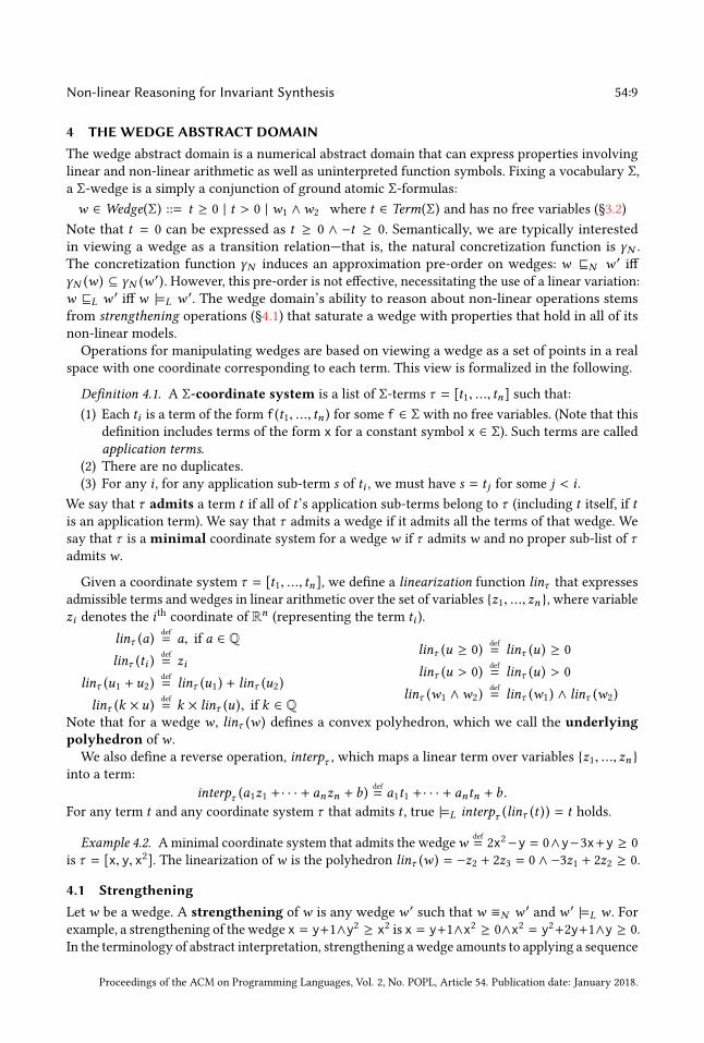
4 THEWEDGE ABSTRACT DOMAINThe wedge abstract domain is a numerical abstract domain that can express properties involving
linear and non-linear arithmetic as well as uninterpreted function symbols. Fixing a vocabulary Σ,a Σ-wedge is a simply a conjunction of ground atomic Σ-formulas:
w ∈ Wedge(Σ) ::= t ≥ 0 | t > 0 | w1 ∧w2 where t ∈ Term(Σ) and has no free variables (§3.2)
Note that t = 0 can be expressed as t ≥ 0 ∧ −t ≥ 0. Semantically, we are typically interested
in viewing a wedge as a transition relation—that is, the natural concretization function is γN .The concretization function γN induces an approximation pre-order on wedges: w ⊑N w ′ iffγN (w ) ⊆ γN (w ′). However, this pre-order is not effective, necessitating the use of a linear variation:w ⊑L w ′ iff w |=L w ′. The wedge domain’s ability to reason about non-linear operations stems
from strengthening operations (§4.1) that saturate a wedge with properties that hold in all of its
non-linear models.
Operations for manipulating wedges are based on viewing a wedge as a set of points in a real
space with one coordinate corresponding to each term. This view is formalized in the following.
Definition 4.1. A Σ-coordinate system is a list of Σ-terms τ = [t1, ..., tn] such that:
(1) Each ti is a term of the form f(t1, ..., tn ) for some f ∈ Σ with no free variables. (Note that this
definition includes terms of the form x for a constant symbol x ∈ Σ). Such terms are called
application terms.(2) There are no duplicates.
(3) For any i , for any application sub-term s of ti , we must have s = tj for some j < i .
We say that τ admits a term t if all of t ’s application sub-terms belong to τ (including t itself, if tis an application term). We say that τ admits a wedge if it admits all the terms of that wedge. We
say that τ is a minimal coordinate system for a wedgew if τ admitsw and no proper sub-list of τadmitsw .
Given a coordinate system τ = [t1, ..., tn], we define a linearization function linτ that expresses
admissible terms and wedges in linear arithmetic over the set of variables {z1, ..., zn }, where variablezi denotes the i
thcoordinate of Rn (representing the term ti ).
linτ (a)def
= a, if a ∈ Q
linτ (ti )def
= zi
linτ (u1 + u2)def
= linτ (u1) + linτ (u2)
linτ (k × u)def
= k × linτ (u), if k ∈ Q
linτ (u ≥ 0)def
= linτ (u) ≥ 0
linτ (u > 0)def
= linτ (u) > 0
linτ (w1 ∧w2)def
= linτ (w1) ∧ linτ (w2)
Note that for a wedge w , linτ (w ) defines a convex polyhedron, which we call the underlyingpolyhedron ofw .
We also define a reverse operation, interpτ , which maps a linear term over variables {z1, ..., zn }into a term:
interpτ (a1z1 +· · · + anzn + b)def
= a1t1 +· · · + antn + b .
For any term t and any coordinate system τ that admits t , true |=L interpτ (linτ (t )) = t holds.
Example 4.2. Aminimal coordinate system that admits the wedgewdef
= 2x2−y = 0∧y−3x+y ≥ 0
is τ = [x, y, x2]. The linearization ofw is the polyhedron linτ (w ) = −z2 + 2z3 = 0 ∧ −3z1 + 2z2 ≥ 0.
4.1 StrengtheningLet w be a wedge. A strengthening of w is any wedge w ′ such that w ≡N w ′ and w ′ |=L w . For
example, a strengthening of the wedge x = y+1∧y2 ≥ x2 is x = y+1∧x2 ≥ 0∧x2 = y2+2y+1∧y ≥ 0.
In the terminology of abstract interpretation, strengthening awedge amounts to applying a sequence
Proceedings of the ACM on Programming Languages, Vol. 2, No. POPL, Article 54. Publication date: January 2018.

54:10 Zachary Kincaid, John Cyphert, Jason Breck, and Thomas Reps
of reductive operators, each of which over-approximates the lower closure operator induced by
the Galois insertion of the powerset lattice of non-linear models into the powerset lattice of linear
models [Granger 1992]. This section presents techniques for strengthening wedges, presented in
two parts: first, inferring implied equalities; second, inferring implied inequalities.
4.1.1 Equalities. Let τ = [t1, ..., tn] be a coordinate system and letw be an admissible wedge of
τ . Let P denote the underlying polyhedron ofw , and let aff(P ) denote a basis for the vector space{ [b0 b1 ... bn
]: ∀
[a1 ... an
]∈ P .b1a1 +· · · + bnan + b0 = 0
}.
aff(P ) is a representation of the set of affine equations that are satisfied by all points in P ; it can be
computed easily from a constraint representation of P . Define I(w,τ ) to be the ideal generated by
aff(P ) and the definitional equalities encoding multiplication and reciprocal coordinates:
I(w,τ )def
=
⟨ {b1z1 + ... + bnzn + b0 : [b0 b1 ... bn
]∈ aff(P )}
∪{zi − linτ (s )linτ (s ′) : ti = s × s ′}∪{linτ (s )zi − 1 : ti = s−1 ∧w |=L ¬(s = 0)}
⟩For any ideal I ⊆ Q[z1, ..., zn] and admissible terms s and t , we write I |= s = t iff (linτ (s ) −
linτ (t )) ∈ I . We say that I is congruence closed if for all terms ti = f(s1, ..., sm ) and tj = f(s ′1, ..., s ′m ) of
τ such that for all i we have I |= s1 = s′1, ..., I |= sm = s
′m thenwe have I |= f(s1, ..., sm ) = f(s ′
1, ..., s ′m ).
The congruence closure of an ideal I is the smallest congruence-closed ideal that contains I . We say
that a wedgew is equationally saturated in τ if for every degree-1 polynomial a1z1 + ... + anzn + bin the congruence closure of the ideal I(w,τ ) vanishes on the underlying polyhedron of w . The
equational saturation of w is the unique (up to ≡L) equationally saturated wedge w ′ such that
w ≡N w ′ and for all equationally saturatedw ′′ such thatw ≡N w ′′ we havew ′′ |=L w′. A procedure
for computing the equational saturation of a wedge is given as Algorithm 1.
Example 4.3. Consider the wedge w = (x × 2x = v ∧ v ≤ (2y + 1) × y ∧ x = y ∧ x ≤ 0) underthe coordinate system τ = [v, x, y, 2x, x × 2x, 2y, (2y + 1) × y]. The association between terms and
coordinates (defined by τ ) is as follows:z1 : v z2 : x z3 : y z4 : 2
x z5 : x × 2x z6 : 2
y z7 : (2y + 1) × y
The underlying polyhedron P ofw is z5 = z1 ∧ z1 ≤ z7 ∧ z2 = z3 ∧ z2 ≤ 0, and the ideal I(w,τ ) is:
I(w,τ )def
= ⟨z5 − z1, z2 − z3︸ ︷︷ ︸aff(P )
, z5 − z2z4, z7 − (z6 + 1)z3︸ ︷︷ ︸Definitional equalities
⟩ .
We will now illustrate Algorithm 1 on the wedge w . First we compute a (degrevlex) Gröbner
basis for I(w,τ ): G = {z5 − z1, z3 − z2, z2z4 − z1, z2z6 − z7 + z2, z1z6 − z4z7 + z2z4} and set the active
coordinates to be {4, 6}, the ones corresponding to the terms 2xand 2
y.
First iteration of the outer loop: When processing coordinate 4 in the inner loop, we add the
mapping CC[2z2] := z4 to CC , indicating that the representative for the term 2z2is z4. We then
process coordinate 6, and find that the term (redG (2))redG (z3 ) = 2z2already has a representative
(z4), and add z6 − z4 to B (i.e., we conclude from the fact that x = y that 2x = 2
y). We add the
equation 2y − 2
x = 0 to w and compute a Gröbner basis for the ideal generated by G and B:G = {z5 − z1, z3 − z2, z6 − z4, z2z4 − z1, z7 − z2 − z1}. Since B contains a non-trivial polynomial,
namely z6 − z4, we continue to a second iteration.
Second iteration of the outer loop: Since the two application terms 2xand 2
ywere identified in the
previous iteration, the inner loop does not produce any new equations. However, the Gröbner basis
G changed in the previous iteration (in particular, it now contains z7−z2−z1). Since redG (z7) = z2+z1,we add the equation (2y+1)×y = v+x tow (line 17). Sincew contains the inequation v ≤ (2y+1)×yand (now) the equation (2y + 1) ×y = v+x, we have v ≤ v+x and thus 0 ≤ x; sincew also contains
x ≤ 0, we have x = 0. Thus, the underlying polyhedron ofw is z5 = z1 ∧ z1 ≤ z7 ∧ z2 = z3 ∧ z2 = 0,
Proceedings of the ACM on Programming Languages, Vol. 2, No. POPL, Article 54. Publication date: January 2018.

Non-linear Reasoning for Invariant Synthesis 54:11
Input :Coordinate system τ = [t1, ..., tn] and a wedgewOutput :Equational saturation ofw in τ
1 G← Gröbner basis (degrevlex) for I(w,τ );
2 active← {i : ti is an application};
3 repeat4 B ← {0};
/* Compute congruence closure. CC maps terms to representative coordinates */
5 CC ← empty map;
6 foreach i in active do7 Let ti = f(s1, ..., sm );
8 Let r j ← redG (linτ (si )) for all j;9 if CC[f(r1, ..., rn )] is defined then
10 zr ← CC[f(r1, ..., rn )];
11 B ← B ∪ {redG (zi − zr )};/* i is represented by zr - it need not be processed again */
12 Remove i from active;13 else14 CC[f(r1, ..., rn )] := zi ;
15 end16 end
/* Add implied linear equations to w. Note that since G is computed w.r.t
degrevlex, the degree of redG (zi ) must be ≤ 1 (i.e., it’s linear) */
17 w ← w ∧( ∧n
i=1 interpτ (zi = redG (zi )))∧
( ∧b ∈B interpτ (b = 0)
);
18 B ← B ∪ {redG (b) : b ∈ basis for I(w,τ )};19 G← Gröbner basis (degrevlex) for ⟨G ∪ B⟩;
20 until B = {0};21 return w
Algorithm 1: Equational saturation
and z2 belongs to I(w,τ ). We add z2 to B and compute a Gröbner basis for the ideal generated by Gand B: G = {z1, z2, z3, z7, z6 − z4}. Since B contains a non-trivial polynomial (z2), we continue to a
third iteration.
Third iteration of the outer loop: Again the inner loop does not produce any new equations. On
line 17 we derive the equations v = 0, x = 0, y = 0, x × 2x = 0, (2y + 1) × y = 0, due to the fact that
G reduces z1, z2, z3, z5, and z7 to 0. Since G reduces every basis polynomial in I(w,τ ) to 0, the loop
exits and the algorithm returns the following (equationally saturated) wedge:
v = x = y = x × 2x = (2y + 1) × y = 0 ∧ 2x = 2
y .
4.1.2 Inequalities. Let τ = [t1, ..., tn] be a coordinate system, letw be an equationally saturated
admissible wedge of τ , and letG be the Gröbner basis of I(w,τ ) (w.r.t degrevlex order). Strengtheningoperations for inferring inequalities that hold in all non-linear models ofw are presented as a set of
inference rules in Fig. 3. The hypotheses and consequences are expressed as polynomial inequalities
in the coordinates z1, ..., zn . A rule may only be applied if hypotheses and consequences are linear
and admissible. Each appearance of linτ (t ) is implicitly guarded by the assumption that τ admits t(so for example, the Floor rule is only applied to floor terms that appear in τ ).
The Interval rule assumes that each function f is associated with a monotone function fivl that
approximates f on intervals (e.g., the interval approximation of multiplication is [a,b] ×ivl [c,d]def
=
Proceedings of the ACM on Programming Languages, Vol. 2, No. POPL, Article 54. Publication date: January 2018.

54:12 Zachary Kincaid, John Cyphert, Jason Breck, and Thomas Reps
Interval
linτ (s1) ∈ [a1,b1] . . . linτ (sm ) ∈ [am ,bm]
linτ (f(s1, ..., sm )) ∈ fivl ([a1,b1], ..., [an ,bn])
Product
linτ (s ) ≥ 0 linτ (t ) ≥ 0
redG (linτ (s )linτ (t )) ≥ 0
Sqare
redG (zizi ) ≥ 0
PowLogLower
linτ (abt ) ≥ linτ (c )linτ (c ) > 0 linτ (b) > 1
linτ (logb (a)) + linτ (t ) ≥ linτ (logb (c ))
Mod
t ≥ 0
0 ≤ linτ (mod (s, t )) ≤ linτ (t ) − 1
PowLogUpper
linτ (c ) ≥ linτ (abt )linτ (a) > 0 linτ (b) > 1
linτ (logb (c )) ≥ linτ (logb (a)) + linτ (t )
Floor
linτ (s ) − 1 < linτ (⌊s⌋) ≤ linτ (s )
Fig. 3. Inference rules for implied inequalities
Input :Σ-wedgew and sub-vocabulary Σ′ ⊆ ΣOutput :Σ′-wedgew ′ withw |=N w ′
1 τ = [t1, ..., tn]← minimal coord. system admittingw ;
2 safe← empty map;
3 for i = 1 to n do4 if ti ∈ Term(Σ′) then5 safe[i]← ti ;
6 end7 end8 repeat9 {i1, ..., ik } ← dom(safe);
10 unsafe← {zi : i ∈ {1, ...,n} \ dom(safe)};11 G← Gröbner basis (elim. order ⪯unsafe) for I(w,τ );
12 for i ∈ unsafe do13 Let ti = f(s1, ..., sm );
14 Let r j ← redG (linτ (sj )) for all j;15 if f ∈ Σ′ and r j ∈ Q[zi1 , ..., zik ] for all j then16 s ′j ← r j with each ziℓ replaced by safe[iℓ];17 safe[i]← f(s ′
1, ..., s ′m )
18 end19 end20 until dom(safe) ∩ unsafe = ∅;
// Polyhedral projection
21 P ← project(linτ (w ), {zi : i ∈ dom(safe)});22 Let Az ≥ b be a constraint representation of P ;
23 w ′ ← Az ≥ b with each zi replaced by safe[i];24 returnw
Algorithm 2: Projection
[min{ac,ad,bc,bd },max{ac,ad,bc,bd }]). The interval constraints in the hypothesis of the rule are
computed using linear programming.
Unlike the equational inference rules, which we can apply until the wedge is saturated, the
inequality inference rules can be applied indefinitely without ever converging. To enforce termi-
nation, we use a simple heuristic: we apply each inference rule in sequence (first we apply the
Interval rule for every term, then the Product rule for every pair of inequalities, ...), and do not
use the consequence of one application of a rule as a hypothesis for the next (e.g., if an inequality
was derived via the Product rule, it may not later be used as the hypothesis of another application
of the Product rule). As a consequence, our algorithm for strengthening a wedge is not complete
with respect to the inference rules (i.e., there are inequations that can be deduced by the inference
rules that will not be be deduced by a single run of the strengthening algorithm).
4.2 Basic Operations on WedgesWe now define some basic operations for manipulating wedges: pseudo-join, meet, widening, and
projection.
Letw1 andw2 be wedges. The pseudo-join ofw1 andw2 is a wedge that is an upper bound of
w1 andw2 with respect to the ordering |=N (it is not, however, a least upper bound with respect
to |=N , which is not computable). We compute the pseudo-joinw1 ⊔̃w2 by first finding a minimal
Proceedings of the ACM on Programming Languages, Vol. 2, No. POPL, Article 54. Publication date: January 2018.

Non-linear Reasoning for Invariant Synthesis 54:13
coordinate system τ that admits both w1 and w2, strengthening both within τ to get wedges w ′1
andw ′2, and setting
w1 ⊔̃w2
def
= interpτ (linτ (w′1) ⊔L linτ (w ′2))
where ⊔L denotes polyhedral join. Observe that due to the strengthening operation,w1 ⊔̃w2 is not
necessarily an upper bound with respect to |=L .
Example 4.4. Consider the wedges y ≥ 1 ∧ y2 ≥ x and 0 ≥ x . A coordinate system admitting
both wedges is [x ,y,y2]. Strengthening y ≥ 1 ∧ y2 ≥ x yields y ≥ 1 ∧ y2 ≥ x ∧ y2 ≥ y, andstrengthening 0 ≥ x yields 0 ≥ x ∧ y2 ≥ 0. The pseudo-join is y2 ≥ x ∧ y2 ≥ 0. Notice that
0 ≥ x ̸ |=L y2 ≥ x ∧ y2 ≥ 0.
Unlike the least upper bound, greatest lower bounds of wedges are exact and easily computed.
The meetw1 ⊓w2 is simply the conjunction:w1 ⊓w2
def
= w1 ∧w2.
Widening. In contrast to conventional methods, the program analysis proposed in this paper makes
no use of widening in the analysis of loops: a loop is analyzed by extracting recurrences and
computing closed forms. However, the interprocedural framework for compositional recurrence
analysis does make use of widening when analyzing functions with non-linear recursion (more than
one recursive call on some path through the function) [Kincaid et al. 2017]. Thus for completeness,
we will define the widening operator for wedges.
Like the pseudo-join operation, the widening operation of wedges relies on the operations of
their underlying polyhedra. Unlike pseudo-join, the dimension of the coordinate system must
decrease rather than increase. Let τ1 and τ2 be minimal coordinate systems admitting w1 and w2,
respectively. Compute a coordinate system τ that contains only the terms that are common to both
τ1 and τ2—w.l.o.g. assume that it is a prefix of both τ1 and τ2. We definew1▽w2 as
w1▽w2
def
= interpτ (projectL (linτ1 (w1), |τ |)▽LprojectL (linτ2 (w2), |τ |))
where projectL (P ,n) denotes the projection of a polyhedron onto its first n dimensions and ▽Ldenotes polyhedral widening.
Projection. Let Σ′ be a sub-vocabulary of Σ. The result of projecting a Σ-wedge w onto Σ′ is aΣ′-wedgew ′ such thatw |=N w ′. While sometimes we wish to eliminate function symbols of arity
≥ 1, most commonly we are interested in the case where Σ and Σ′ differ by a set X of constant
symbols, in which case projecting onto Σ′ results in an over-approximation of the formula (∃X .w ).A projection algorithm is given as Algorithm 2. It operates as follows. Letw be a Σ-wedge and
let τ = [t1, ..., tn] be a minimal coordinate assignment admittingw . If ti is a Σ′-term, we mark i as
safe and associate i with ti ; otherwise, it is unsafe. We then compute the Gröbner basis for the ideal
I(w,τ ) w.r.t. an an elimination ordering for {zi : ti is unsafe}. We then traverse the unsafe terms
ti = f(s1, ..., sm ): if every coordinate in redG (linτ (sj )) is safe for all sj , we mark i safe and associate
it with an equivalent Σ′-term. We iterate this process until no more coordinates are marked safe.
We then use polyhedral projection to eliminate the unsafe dimensions, and then replace the safe
dimensions with their associated Σ′-terms to obtain a Σ′ wedgew ′.
4.3 Symbolic AbstractionSymbolic abstraction is the key operation supported by the wedge domain, and the foundation of
our method for extracting recurrence relations from transition formulas (see §5). Given a formula
ϕ, symbolic abstraction computes a wedge w that over-approximates it (that is, ϕ |=N w) and is
as precise as possible (noting that the latter part of the specification is informal, since the mostprecise wedge is not necessarily computable or even well defined). Phrased differently, symbolic
abstraction computes a system of equations and inequations that are implied by a given formula.
Proceedings of the ACM on Programming Languages, Vol. 2, No. POPL, Article 54. Publication date: January 2018.
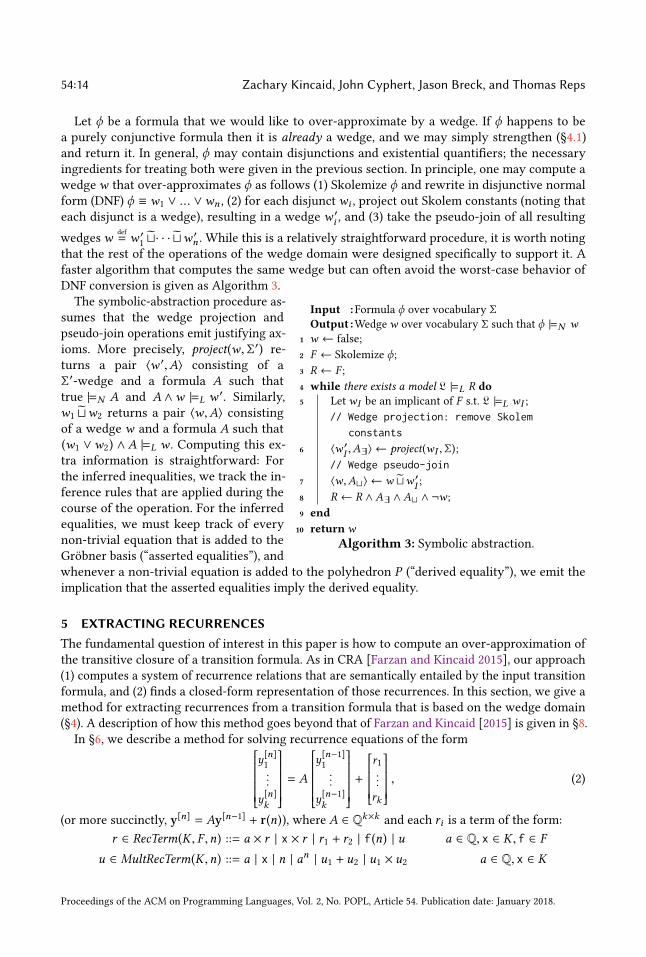
54:14 Zachary Kincaid, John Cyphert, Jason Breck, and Thomas Reps
Let ϕ be a formula that we would like to over-approximate by a wedge. If ϕ happens to be
a purely conjunctive formula then it is already a wedge, and we may simply strengthen (§4.1)
and return it. In general, ϕ may contain disjunctions and existential quantifiers; the necessary
ingredients for treating both were given in the previous section. In principle, one may compute a
wedgew that over-approximates ϕ as follows (1) Skolemize ϕ and rewrite in disjunctive normal
form (DNF) ϕ ≡ w1 ∨ ... ∨wn , (2) for each disjunctwi , project out Skolem constants (noting that
each disjunct is a wedge), resulting in a wedge w ′i , and (3) take the pseudo-join of all resulting
wedgeswdef
= w ′1⊔̃· · · ⊔̃w ′n . While this is a relatively straightforward procedure, it is worth noting
that the rest of the operations of the wedge domain were designed specifically to support it. A
faster algorithm that computes the same wedge but can often avoid the worst-case behavior of
DNF conversion is given as Algorithm 3.
Input :Formula ϕ over vocabulary ΣOutput :Wedgew over vocabulary Σ such that ϕ |=N w
1 w ← false;
2 F ← Skolemize ϕ;
3 R ← F ;
4 while there exists a model L |=L R do5 LetwI be an implicant of F s.t. L |=L wI ;
// Wedge projection: remove Skolem
constants
6 ⟨w ′I ,A∃⟩ ← project(wI , Σ);
// Wedge pseudo-join
7 ⟨w,A⊔⟩ ← w ⊔̃w ′I ;
8 R ← R ∧A∃ ∧A⊔ ∧ ¬w ;
9 end10 returnw
Algorithm 3: Symbolic abstraction.
The symbolic-abstraction procedure as-
sumes that the wedge projection and
pseudo-join operations emit justifying ax-
ioms. More precisely, project(w, Σ′) re-
turns a pair ⟨w ′,A⟩ consisting of a
Σ′-wedge and a formula A such that
true |=N A and A ∧w |=L w′. Similarly,
w1 ⊔̃w2 returns a pair ⟨w,A⟩ consistingof a wedge w and a formula A such that
(w1 ∨w2) ∧A |=L w . Computing this ex-
tra information is straightforward: For
the inferred inequalities, we track the in-
ference rules that are applied during the
course of the operation. For the inferred
equalities, we must keep track of every
non-trivial equation that is added to the
Gröbner basis (“asserted equalities”), and
whenever a non-trivial equation is added to the polyhedron P (“derived equality”), we emit the
implication that the asserted equalities imply the derived equality.
5 EXTRACTING RECURRENCESThe fundamental question of interest in this paper is how to compute an over-approximation of
the transitive closure of a transition formula. As in CRA [Farzan and Kincaid 2015], our approach
(1) computes a system of recurrence relations that are semantically entailed by the input transition
formula, and (2) finds a closed-form representation of those recurrences. In this section, we give a
method for extracting recurrences from a transition formula that is based on the wedge domain
(§4). A description of how this method goes beyond that of Farzan and Kincaid [2015] is given in §8.
In §6, we describe a method for solving recurrence equations of the form
y[n]1
...
y[n]k
= A
y[n−1]1
...
y[n−1]k
+
r1...
rk
, (2)
(or more succinctly, y[n] = Ay[n−1] + r(n)), where A ∈ Qk×k and each ri is a term of the form:
r ∈ RecTerm(K , F ,n) ::= a × r | x × r | r1 + r2 | f(n) | u a ∈ Q, x ∈ K , f ∈ F
u ∈ MultRecTerm(K ,n) ::= a | x | n | an | u1 + u2 | u1 × u2 a ∈ Q, x ∈ K
Proceedings of the ACM on Programming Languages, Vol. 2, No. POPL, Article 54. Publication date: January 2018.

Non-linear Reasoning for Invariant Synthesis 54:15
while(*) {if(*) { x := 2x + y + i }else { y := x + 2y + i }i := i + 1j := j + x
}
(a) Example program
*....,
(x′ = 2x + y + i ∧ y′ = y∨x′ = x ∧ y = x + 2y + i
)∧i′ = i + 1∧j′ = j + x′
+////-
(b) Loop-transition formula
*.,
x′ + y′ = 2x + 2y + i∧i′ = i + 1∧j′ = j + x′
+/-
(c) Loop-transition wedge
Fig. 4. A loop, along with its transition formula and transition wedge
whereK is a set of symbolic constants (initial values of program variables) and F is a set of implicitly
interpreted functions (IIFs). The closed forms computed by the recurrence solver have the same
form as RecTerm above.
In general, the behavior of a loop cannot be expressed as such a system of recurrence equations:
loopsmay have non-deterministic assignments, conditional branches, nested loops, etc. The question
is how we can exploit a solver for recurrences of this form, even though the loop itself does not have
such a description. Our solution involves extracting multiple systems of recurrences for the same
loop, where each system approximates some aspect of the dynamics of the loop. In the following,
we present three different mechanisms for extracting recurrences from a transition formula, each
building on the last.
The recurrence-extractionmechanisms all assume a wedge representation of the loop body, which
eliminates the need to deal with disjunction and existentially quantified variables (both of which
are present in transition formulas). Thus, the first step we take in computing recurrences entailed by atransition formula ϕbody is to find an over-approximating wedgewbody using the symbolic-abstractionprocedure from §4.3 (Algorithm 3).
Before proceeding to the recurrence-extraction algorithms, we will formalize the problem set-
up that is common to all. We fix ϕbody to be a loop-body transition formula, and wbody to be a
wedge that over-approximates it. Suppose that PVar is a set of constant symbols that represent
program variables, and PVar′is a disjoint set of “primed copies” of program variables. Suppose Σ
is a vocabulary containing PVar, PVar′, and ΣN . Fix a Σ-wedgewbody that over-approximates the
transition relation of a loop body. Let τ = [t1, ..., tn] be a coordinate system admittingwbody. Without
loss of generality, suppose that the terms t1, ..., tm correspond to the program variables in PVar
and the terms tm+1, ..., t2m correspond to the program variables in PVar′. We use x def
= [z1, ..., zm] to
denote the vector of variables corresponding to PVar and x′ def
= [zm+1, ..., z2m] to denote the vector
of variables corresponding to PVar′.
5.1 Affine RecurrencesAn affine recurrence is a recurrence for a linear combination of program variables. Our goal is
to compute matrices A ∈ Qk×m and B ∈ Qk×k and a vector c ∈ Qk such that wbody |=L Ax′ =BAx + c. The relation Ax′ = BAx + c defines a set of affine recurrences for the linear combinations
in Ax. Moreover, we want the affine space consisting of all valuations of x and x′ that satisfyAx′ = BAx + c to be least (in the sense that if A′,B′, c′ satisfy wbody |=L A′x′ = B′A′x + c′, thenwe have Ax′ = BAx + c |=L A′x′ = B′A′x + c′). Suppose that cl is a closed-form solution to the
system of recurrence equations yn = Byn−1 + c (which matches the form in Eqn. (2)), in the sense
that y[n] = By[n−1] + c ⇐⇒ y[n] = cl(y[0],n). Then the transitive closure of ϕbody must entail
∃n ≥ 0.Ax′ = cl(Ax,n).As a motivating example, consider the loop from Fig. 4(a) and the associated transition formula
and wedge. Observe that (1) the loop is non-deterministic, and there is no exact representation of
Proceedings of the ACM on Programming Languages, Vol. 2, No. POPL, Article 54. Publication date: January 2018.

54:16 Zachary Kincaid, John Cyphert, Jason Breck, and Thomas Reps
the closed form of the variables x or y, and (2) despite the fact that there is an apparently recursive
assignment to the variable j, there is no exact closed form for j because it depends on variable x,for which there is no closed form. For this example, the best
3affine recurrence is
[1 0 0 0
0 0 1 1
]
i′
j′
x′
y′
=
[1 0
1 2
] [1 0 0 0
0 0 1 1
]
ijxy
+
[1
0
](3)
(or more simply, i′ = i + 1 and (x′ + y′) = 2(x + y) + i). Note how the second row of matrix A in
Eqn. (3) creates the linear combinations x′ + y′ and x + y in the latter recurrence equation.
The best affine recurrence entailed by w can be computed via successive approximation. We
begin by explaining the procedure in the abstract, and return to the concrete example below. The
first approximation A1x′ = M1x + c1 is merely the constraint representation of the affine hull of
the underlying polyhedron ofw , projected onto the first 2m dimensions (corresponding to the xand x′ symbols). IfM1 factors as BA1, then we are done: the best affine recurrence entailed bywis A1x′ = BA1x + c1. If M1 does not factor as BA1, then the equation A1x′ = M1x + c1 cannot beinterpreted as a recurrence. (The rowspace of A1 must contain the rowspace ofM1—intuitively, the
terms that appear on the right-hand side of a recurrence equation must be linear combinations of
terms that appear on the left.) Thus, we compute a second approximation A2x′ = M2x+ c2. For anyapproximation i , the (i + 1)th approximation is computed from the ith by finding a matrix Ti whoserows form a basis for the vector space {v : ∃u.uAi = vBi } and taking Ai+1 = TiAi , Mi+1 = TiMi ,
and ci+1 = Tici . Eventually this process must reach a fixpoint, because each step decreases the
dimension of the rowspace of Ai by at least 1.
Returning to our running example Fig. 4, the first approximation is essentially just the wedge
Fig. 4(c) itself:
0 0 1 1
1 0 0 0
0 1 −1 0
︸ ︷︷ ︸A1
i′
j′
x′
y′
=
1 0 2 2
1 0 0 0
0 1 0 0
︸ ︷︷ ︸M1
ijxy
+
0
1
0
︸︷︷︸c1
Observe that the rowspace ofA1 does not contain
[0 1 0 0
], the third row ofM1 (i.e., j appears
on the right-hand side of an equation but we cannot isolate j′ on the left). We find a matrix T1whose rows generate the space {v : ∃u.uA1 = vB1} pictured below to the left (intuitively, T1 isa linear transformation that projects out j), and multiply both sides of the equation to get the
equation pictured below to the right:
[0 1 0
1 0 0
]
︸ ︷︷ ︸T1
[1 0 0 0
0 0 1 1
]
︸ ︷︷ ︸A2
i′
j′
x′
y′
=
[1 0 0 0
1 0 2 2
]
︸ ︷︷ ︸M2
ijxy
+
[1
0
]
︸︷︷︸c2
The rowspace of A2 does contain the rowspace ofM2, so are done. We factorM2 as BA2 and obtain
the affine recurrence shown in Eqn. (3).
5.2 Stratified RecurrencesConsider the simple loop while(*){ y += x*x; x++; }. The affine recurrence extracted by
the algorithm in the preceding section is x′ = x + 1: no recurrence is extracted for y because itsrecurrence has a non-linear dependence on x. However, because there is no circular dependence of
3“Best” in the sense that it generates the least affine space. The affine space is unique, but its representation as a system of
equations is not. However, the representation is irrelevant for our purposes.
Proceedings of the ACM on Programming Languages, Vol. 2, No. POPL, Article 54. Publication date: January 2018.

Non-linear Reasoning for Invariant Synthesis 54:17
x on y, we can arrange the recurrences into strata and leverage the closed form of x to compute a
closed form for y:
Stratum Recurrence Closed form
0 x′ = x + 1 x[n] = x[0] + n
1 y′ = y + x × xy[n] = y[0] +
∑n−1i=0 x[i] = y[0] +
∑n−1i=0 (x
[0] + i )2
= y[0] + n/6 − n2/2 + n3/3 − nx[0] + n2x[0] + n(x[0])2
More generally, we can compute a sequence of stratified recurrences such that each recurrence in
the sequence may have non-linear dependencies on previous terms in the sequence:
wbody |=L A0x′ = B0A0x + cwbody |=L A1x′ = B1A1x + p1 (A0x)
...wbody |=L Aix′ = BiAix + pi (A0x, ...,Ai−1x)
where A0x′ = B0A0x + c is an affine recurrence and each pi (A0x, ...,Ai−1x) is a polynomial over
the terms in A0x, ...,Ai−1x. For each stratum j, the closed form clj is computed as the solution to a
single matrix recurrence (of the form in Eqn. (2)) by substituting closed forms of previous strata
into the next:
y[n]0= B0y
[n−1]0
+ c ⇐⇒ y[n]0= cl0 (y
[0]
0,n)
y[n]1= B1y
[n−1]1
+ p1 (cl0 (y[n]0,n)) ⇐⇒ y[n]
1= cl1 (y
[0]
0, y[0]
1,n)
...
y[n]i = Biy[n−1]i + pi (cl0 (y
[n]0,n), ..., cli−1 (y
[n]0, ..., y[n]i−1,n)) ⇐⇒ y[n]i = cli (y
[0]
0, ..., y[0]i−1,n)
Observing that substitution ofMultRecTerms into a polynomial yields aMultRecTerm, this procedure
works as long as no cli (y[0]
0, ..., y[0]i−1,n) contains an IIF.
The procedure for extracting stratified recurrences similarly proceeds iteratively on strata,
beginning at stratum 0 (the best affine recurrence satisfied by the input wedge, as computed in §5.1),
and continuing until reaching a stratum where no new recurrences are found. For each stratum i ,we compute the recurrence equation
Aix′ = BiAix + pi (A0x, ...,Ai−1x)as follows. Let T = {t1, ..., tk } be a set consisting of all linear terms of the form ax, where a is arow of one of the matrices A0, ..., Ai−1; T corresponds to the set of linear terms for which there is a
recurrence equation in some strata < i (and thus, we know a closed form for each tj ). For each term
tj ∈ T create a fresh variable r j and define Ii to be the ideal generated by I(wbody,τ ) along with the
(linear) polynomials {r j − tj : 1 ≤ j ≤ k }. Compute a Gröbner basis Gi for Ii w.r.t. an elimination
order for {z2m+1, ..., zn }, with the r variables ordered before the z variables. Recall that the variablesz2m+1, ..., zn correspond to non-linear terms over program variables, so reduction by Gi projects
out non-linear terms over the program variables, but in doing so may introduce polynomials of the
new r variables (which is desirable, since those are the polynomials for which we can compute
closed forms). Compute an initial system of equations
Ai,1x′ = Mi,1x + pi,1where Ai,1 andMi,1 are rational matrices, and p is a vector of polynomials in Q[t1, ..., tk ] by taking
the constraint representation of the affine hull of the underlying polyhedron ofw , reducing each
equation by Gi , collecting the subset of equations that have the appropriate form, and finally
replacing each (z and r ) variable with its corresponding (x, x’, and ti ) term. Then perform the same
fixpoint algorithm from §5.1 to reduce this system of equations to a system of recurrence equations
of the form Aix′ = BiAix + pi , and proceed to the next stratum i + 1.
Proceedings of the ACM on Programming Languages, Vol. 2, No. POPL, Article 54. Publication date: January 2018.

54:18 Zachary Kincaid, John Cyphert, Jason Breck, and Thomas Reps
5.3 Recurrence InequationsIn §5.1 and §5.2, we describedmethods for describing the exact behavior of linear terms over program
variables using recurrence equations. In this sub-section, our goal shifts to finding inequations thatbound linear terms. Our goal is to compute a system of recurrence inequations
wbody |=L Ax′ ≤ BAx + p(A0x, ...,Akx)where A ∈ Qk×m is rational matrix, B ∈ Qk×k is a non-negative matrix (that is, a matrix with no
negative entries), and p(A0x, ...,Akx) is a polynomial over A0x, ...,Akx, where A0, ...,Ak are as in
§5.2.
The procedure for extracting recurrence inequations operates similarly to the one for affine
recurrences, except that rather than finding some i such that Ai and Mi generate the same row
space, we require that Ai andMi generate the same cone. Given a matrix A with rows a1, ..., ak , the(convex) cone generated by the rows of A is as follows:
cone(A) def
= {λ1a1 +· · · + λkak : λ1 ≥ 0, ..., λk ≥ 0}
The requirement that Ai andMi generate the same cone guarantees that there exists a factorization
Mi = BAi where B is non-negative. A second complication is that the iterative algorithm may
fail to terminate because the lattice of polyhedra (in contrast to the lattice of vector spaces) has
infinite ascending chains. We use polyhedral widening to guarantee termination of the successive-
approximation algorithm.
6 OPERATIONAL CALCULUS RECURRENCE SOLVING6.1 IntroductionOperational calculus [J.-G.-M. 1983] is a technique for transforming a problem in analysis into
an algebraic problem. Differencing and summation correspond to algebraic operators in a certain
underlying algebra. Most commonly, operational-calculus techniques are used to solve differential
equations. However, using the operational-calculus algebra of Berg [1967, Ch. II] it is possible to
solve recurrence relations using operational calculus. The analysis problem of solving a recurrence
equation is transformed into an equation or equation system, which is then solved by algebraic
manipulations. A solution to the original problem can be read out of a solution to the algebraic
problem.
6.1.1 The Ring of Functions. In this section, we review the univariate operational calculus of
Berg [1967, Ch. II]. The ring of functions R is defined as Rdef
= (R,+, ·, 0, 1), where R = N→ Q.4
It is often helpful to consider a ring element r ∈ R as an infinite sequence ⟨r [0], r [1], r [2], . . .⟩.For r ∈ R, we use both r (i ) and r [i] to denote the ith element of r . (We use r (i ) when we wish to
emphasize that r is the function λi .r (i ), and r [i] when we wish to emphasize that r is the sequence⟨r [i]⟩.)
Ring addition is pointwise addition: for all a,b ∈ R, a + bdef
= λi .a(i ) + b (i ), so the additive
identity element, 0, is λi .0 = ⟨0, 0, 0, . . .⟩. Ring multiplication is the following convolution-product
difference:
Definition 6.1. For all a,b ∈ R,
a · bdef
= λn.n∑ν=0
a[ν ]b[n−ν ] −n−1∑ν=0
a[ν ]b[n−1−ν ]. (4)
4Berg uses N→ C, where C is the set of complex numbers. However, our goal is to compute closed forms for recurrences
that can be expressed in the term language of the logic defined in §3.2, which requires using Q.
Proceedings of the ACM on Programming Languages, Vol. 2, No. POPL, Article 54. Publication date: January 2018.

Non-linear Reasoning for Invariant Synthesis 54:19
We will often omit multiplication operators, and write a · b as ab. The multiplicative identity
element, 1, is λi .1 = ⟨1, 1, 1, . . .⟩. It is easy to show that multiplication is commutative and that
multiplication distributes over addition [Berg 1967, §7].
The constant elements of R are those of the form cdef
= λn.c = ⟨c, c, c, . . .⟩. When either argument
of a multiplication is a constant, ring multiplication acts like scalar multiplication: for all b ∈ R,c · b = λn.cb[n]. When both arguments are scalars, ring multiplication is isomorphic to ordinary
multiplication: c · d = cd .It is sometimes useful to write Eqn. (4) as
a · bdef
= λn.n−1∑ν=0
a[ν ] (b[n−ν ] − b[n−1−ν ]) + a[n]b[0]. (5)
Id denotes the identity function λn.n = ⟨0, 1, 2, . . .⟩. Using Eqn. (5), note that for all a ∈ R,
Id · a = a · Id = λn.n−1∑ν=0
a[ν ] ((n − ν ) − (n − 1 − ν )) + a[n]0 = λn.n−1∑ν=0
a[ν ].
In other words, Id acts as a summation operator, producing the sequence of (exclusive) partial sums
of a. For instance, Id · Id = ⟨0, 0, 1, 3, 6, 10, 15, . . .⟩ = λn.(n2
).5
Let vdef
= ⟨0, 1, 1, 1, . . .⟩. Let c[n] denote an arbitrary infinite sequence ⟨c[0], c[1], . . .⟩. Then
v · c[n] = λn.
0 if n = 0
c[n−1] if n ≥ 1
and hence ring multiplication by v performs a right shift (and ring multiplication by vm performs
a right shift of c[n] bym places.).
6.1.2 The Field of Operators. Ring R has no divisors of 0, and hence can be extended to a field
Fdef
= (F ,+, ·,−, −1, 0, 1) An element of F is called an operator. Some operators are elements of R;however, there are interesting operators that are not members of R. For instance, the equation
qv = 1 (6)
has no solution in R. However, because v , 0, there is an operator q ∈ F that solves Eqn. (6).
Intuitively, q should be a left-shift operator.
As Berg points out [Berg 1967, §8], an operator can be interpreted as a sequence with a finite
number of non-zero elements at negative-index positions (whereas a ring element is a sequence
with no non-zero elements at negative-index positions). Therefore, it is easy to show that the
appropriate representation for q, the operator that solves Eqn. (6), is
. . . −2 −1 0 1 2 3 . . .
q = . . . 0 1 1 1 1 1 . . .
Let y[n] denote an arbitrary infinite sequence ⟨y[0],y[1], . . .⟩, and let y[n+1] denote ⟨y[1],y[2], . . .⟩.The following general formula expresses y[n+1] in terms of y[n], y[0], and q. It works by multiplying
y[n] by q to shift the sequence to the left by one position, and subtracting away the value that
would otherwise appear at index position −1, giving us y[n+1]:
y[n+1] = q · y[n] − (q − 1)y[0]. (7)
5As is standard, for n ≥ k , the binomial coefficient
(nk
)denotes
n!k !(n−k )! . We define
(0
0
)= 1 and, for all k > n,
(nk
)= 0.
Proceedings of the ACM on Programming Languages, Vol. 2, No. POPL, Article 54. Publication date: January 2018.

54:20 Zachary Kincaid, John Cyphert, Jason Breck, and Thomas Reps
We can depict some of the infinite sequences that appear in Eqn. (7) as follows:
. . . −2 −1 0 1 2 3 . . .
y[n] = . . . 0 0 y[0] y[1] y[2] y[3] . . .y[n+1] = . . . 0 0 y[1] y[2] y[3] y[4] . . .q · y[0] = . . . 0 y[0] y[1] y[2] y[3] y[4] . . .
(q − 1)y[0] = . . . 0 y[0] 0 0 0 0 . . .
Henceforth, sequences like the ones above will be written as follows:
y[n] = ⟨y[0],y[1],y[2],y[3], . . .⟩y[n+1] = ⟨y[1],y[2],y[3],y[4], . . .⟩
q · y[n] = ⟨y[0] ∥ y[1],y[2],y[3],y[4], . . .⟩(q − 1)y[0] = ⟨y[0] ∥ 0, 0, 0, 0, . . .⟩
where ∥ is used to separate the negative-index positions (if any) from the non-negative positions.
The values at all negative-index positions that are not shown are assumed to be 0.
Using this notation, the operators q and (q − 1) have the sequences shown below:
q = ⟨1 ∥ 1, 1, 1, 1, . . .⟩ (q − 1) = ⟨1 ∥ 0, 0, 0, 0, . . .⟩
Eqn. (7) can be generalized to create y[n+m] = ⟨y[m],y[m+1],y[m+2],y[m+3], . . .⟩ from y[n] asfollows:
y[n+m] = qm · y[n] −m−1∑µ=0
qµ · (q − 1)y[m−1−µ]. (8)
In this case, it is necessary to knock out them values y[0],y[1], . . . ,y[m−1] from positions −m,−m +1, . . . ,−1, respectively. Eqn. (8) can be understood by recognizing that
(q − 1)y[m−1−µ] = ⟨y[m−1−µ] ∥ 0, 0, 0, 0, . . .⟩,
which is then shifted µ positions to the left by qµ .
6.1.3 Translation Rules. In some cases, functions that are expressed in terms of operators can
also be expressed purely in terms of ordinary algebra. For example, consider the functional sequence
λn.αn = ⟨α0,α1,α2, . . .⟩ for n ∈ N and α ∈ Q. By Eqn. (7) and α0 = 1 we have:
αn+1 = qαn − (q − 1)α0
qαn − αn+1 = (q − 1)
αn (q − α ) = (q − 1)
αn =q − 1
q − α
Thus we have a way of translating a recognizable functional sequence in standard algebra to the
operational-calculus algebra. We will write this translation as:
Tn
(q − 1
q − α
)= αn
Fig. 5 shows the above rule along with other useful translation rules.
6.2 Solving First-Order Univariate RecurrencesThe properties of the algebra described in §6.1 give us a nice algebraic way of solving recurrences
of the following form:
y[n+1] = α · y[n] +∑i
fi (n) where fi (n) = polyi (n) ∗ βni and polyi (n) ∈ Q[n] (17)
Algorithm 4 presents a method for solving such univariate recurrences.
Proceedings of the ACM on Programming Languages, Vol. 2, No. POPL, Article 54. Publication date: January 2018.

Non-linear Reasoning for Invariant Synthesis 54:21
Tn(c)= c (9)
Tn*.,
∑k ∈K
дk+/-=
∑k ∈K
Tn (дk ) (10)
Tn(c f
)= cTn ( f ) (11)
Tn
(1
(q − 1)i
)=
(n
i
)(12)
Tn
(q − 1
q − k
)= kn (13)
Tn
(q − 1
(q − k )c+1
)=
(n
c
)kn−c (14)
Tn
(1
q − k
)=
kn − 1
k − 1(15)
Tn
(1
(q − k )c
)=
( nc−1
)− Tn
(1
(q−k )c−1
)k − 1
(16)
Fig. 5. Translation function Tn : F → R. In Eqn. (10) K ⊆ N is some finite index set.
Input :A recurrence inequation r , a variable to solve for y, and an index variable nOutput :The closed form solution for y
1 R ← Simplify r ;
2 OpR ← Translate R into F using Eqn. (8) and T −1n ;
3 OpR ← Solve for y in OpR ;
4 OpR ← Perform partial-fraction decomposition on OpR ;
5 S ← Tn (OpR) ;
6 S ← Simplify S ;
7 return S
Algorithm 4: Univariate Operational Calculus Recurrence Solving
6.2.1 Explanation of Operational Calculus Recurrence Solving. Between each step of the algo-
rithm we simplify expressions using a simplification algorithm, given in Cohen [2003], which
performs standard algebraic simplifications, such as collecting like terms and combining exponents.
Simplification helps to maintain a more canonical form for expression matching in later steps.
Consider how Step 2 of Algorithm 4, translates a recurrence of the form of Eqn. (17). We can use
Eqn. (7) to write y[n+1] as qy[n] − (q − 1)y[0]. For the right-hand side of Eqn. (17), α · y[n] remains
the same, except that the constant α becomes the constant sequence α . What remains to describe is
how we obtain T −1n (∑
i fi (n)).As a quick detour, note that for all the rules in Fig. 5, polynomials are represented using a binomial
operator. Thus we must have an appropriate way to represent polynomials using binomials. This
transformation can be performed via the following relation, where
{dj
}denotes a Stirling number
of the second kind:
nd =d∑j=0
j!
{d
j
}(n
j
)(18)
To perform the translation T −1n (∑
i fi (n)), first note that by Eqn. (10), we can pull the summation
out. We now seek a characterization of T −1n
(polyi (n) ∗ β
ni
). First, consider rewriting polyi (n) using
Eqn. (18), where d = deg(polyi (n)).
fi (n) = βni ∗ polyi (n) = β
ni ∗
d∑j=0
νi, j
(n
j
)=
d∑j=0
β ji ∗ νi, j
(n
j
)βn−ji
We can use the general transformation
T −1n
((n
c
)kn−c
)=
q − 1
(q − k )c+1
Proceedings of the ACM on Programming Languages, Vol. 2, No. POPL, Article 54. Publication date: January 2018.

54:22 Zachary Kincaid, John Cyphert, Jason Breck, and Thomas Reps
to see that every fi (n) can be translated into the following form in the operational-calculus algebra:
T −1n ( fi (n)) =d∑j=0
γi, j (q − 1)
(q − βi )c j
where γi, j is an appropriate constant. Thus, after Step 2 Algorithm 4 produces an equation of the
form
q · y[n] − (q − 1)y[0] = α · y[n] +∑i
d∑j=0
γi, j (q − 1)
(q − βi )ci, j
The algorithm continues, solving the above equation for yn in Step 3.
y[n] =q − 1
q − αy[0] +
∑l
γl (q − 1)
(q − α ) (q − βl )cl
Note the double summation has been replaced by a single summation with a new index, l .Thus, after Step 3, we need to transform all the summands to a form that has a translation rule
in Fig. 5. We can accomplish this goal by performing partial-fraction decomposition on all the
summands (Step 4).
q − 1
q − αy[0] +
∑k
ak
(q − bk )ck
where ak and bk are constants resulting from partial-fraction decomposition, and every ck is a
non-negative integer. After Step 4, the right-hand side of the equation will be a sum of terms, each
of which has a translation rule in Fig. 5 that can be applied to translate the term back into standard
algebra (Step 5). Finally, in Step 6, the algorithm removes binomials and simplifies the result.
The preceding four paragraphs have shown that Algorithm 4 obtains a closed-form solution
to any recurrence of the form given in Eqn. (17). The steps used in Algorithm 4 never get stuck;
i.e., operations such as partial-fraction decomposition in Step 4 can always be performed. In other
words, we have proven the following theorem:
Theorem 6.2. Algorithm 4 is complete for the class of recurrences given in Eqn. (17).
Example 6.3. Consider the following example, which generates an exponential closed form.
y[n+1] = 2y[n] + 3n
Step 2 generates the following equation in F :
q · y[n] − (q − 1)y[0] = T −1n
(2y[n] + 3n
)q · y[n] − (q − 1)y[0] = 2y[n] +
q − 1
q − 3
By Eqn. (11), Eqn. (9), Eqn. (10), Eqn. (13), and Eqn. (7).
After solving for y[n], Step 3 produces
y[n] =q − 1
q − 2y[0] +
q − 1
(q − 3) (q − 2)
Step 4 performs partial-fraction decomposition on the right-hand side of the equation where
appropriate, obtaining
y[n] =q − 1
q − 2y[0] +
2
q − 3−
1
q − 2Finally, Step 5 translates the resultant expression back to standard algebra and the algorithm
performs a final simplification.
y[n] = Tn
(q − 1
q − 2y[0] +
2
q − 3−
1
q − 2
)Proceedings of the ACM on Programming Languages, Vol. 2, No. POPL, Article 54. Publication date: January 2018.
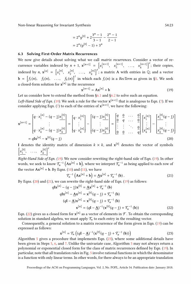
Non-linear Reasoning for Invariant Synthesis 54:23
= 2ny[0] + 2
3n − 1
3 − 1−2n − 1
2 − 1
= 2n (y[0] − 1) + 3n
6.3 Solving First-Order Matrix RecurrencesWe now give details about solving what we call matrix recurrences. Consider a vector of re-
currence variables indexed by n + 1, x[n+1] =[x [n+1]1, x [n+1]
2, . . . , x [n+1]k
] t; their copies,
indexed by n, x[n] =[x [n]1, x [n]
2, . . . , x [n]k
] t; a matrix A with entries in Q; and a vector
b =[f1 (n), f2 (n), . . . , fk (n)
] tin which each fi (n) is a RecTerm as given in §5. We seek
a closed-form solution for x[n] in the recurrence
x[n+1] = Ax[n] + b (19)
Let us consider how to extend the method from §6.1 and §6.2 to solve such an equation.
Left-Hand Side of Eqn. (19). We seek a rule for the vector x[n+1] that is analogous to Eqn. (7). If we
consider applying Eqn. (7) to each of the entries of x[n+1], we have the following:
x[n+1] =
q · x [n]1− (q − 1)x [0]
1
...
q · x [n]k − (q − 1)x [0]k
=
q · x [n]1
...
q · x [n]k
−
(q − 1)x [0]1
...
(q − 1)x [0]k
=
q 0 . . . 0
0 q . . . 0
....... . . 0
0 0 . . . q
x [n]1
...
x [n]k
−
x [0]1(q − 1)
...
x [0]k (q − 1)
= qIx[n] − x[0] (q − 1) (20)
I denotes the identity matrix of dimension k × k , and x[0] denotes the vector of symbols[x [0]1, . . . , x [0]k
] t.
Right-Hand Side of Eqn. (19).We now consider rewriting the right-hand side of Eqn. (19). In other
words, we seek to know T −1n
(Ax[n] + b
), where we interpret T −1n as being applied to each row of
the vector Ax[n] + b. By Eqns. (10) and (11), we have
T −1n
(Ax[n] + b
)= Ax[n] + T −1n (b) . (21)
By Eqns. (20) and (21), we can rewrite the right-hand side of Eqn. (19) as follows:
qIx[n] − (q − 1)x[0] = Ax[n] + T −1n (b)
qIx[n] − Ax[n] = x[0] (q − 1) + T −1n (b)
(qI − A)x[n] = x[0] (q − 1) + T −1n (b)
x[n] = (qI − A)−1 (x[0] (q − 1) + T −1n (b)) (22)
Eqn. (22) gives us a closed form for x[n] as a vector of elements in F . To obtain the corresponding
solution in standard algebra, we must apply Tn to each entry in the resulting vector.
Consequently, a general solution to a matrix recurrence of the form given in Eqn. (19) can be
expressed as follows:
x[n] = Tn((qI − A)−1 (x[0] (q − 1) + T −1n (b))
)(23)
Algorithm 5 gives a procedure that implements Eqn. (23), where some additional details have
been given in Steps 5, 6, and 7. Unlike the univariate case, Algorithm 5 may not always return a
polynomial or exponential closed form for the class of matrix recurrences defined by Eqn. (19). In
particular, note that all translation rules in Fig. 5 involve rational functions in which the denominator
is a function with only linear terms. In other words, for there always to be an appropriate translation
Proceedings of the ACM on Programming Languages, Vol. 2, No. POPL, Article 54. Publication date: January 2018.

54:24 Zachary Kincaid, John Cyphert, Jason Breck, and Thomas Reps
Input :A vector of recurrence variables indexed by n + 1, x[n+1], a matrix A, a vector of recurrencevariables indexed by n, x[n], and an additive vector b
Output :The closed form solution for x[n], in x[n+1] = Ax[n] + b1 b← Simplify b ;
2 Opb← x[0] (q − 1) + T −1n (b) ;3 D← Symbolically calculate (qI − A)−1;4 V← D ∗ Opb;5 V← Convert every entry in V to the form
pq , where p and q are polynomials in Q[q];
6 V← for everypiqi ∈ V, factor qi into its irreducible factors in Q[q];
7 V← for every vi ∈ V, perform partial-fraction decomposition on vi ;
8 S← for every vi ∈ V, replace vi with Tn (vi ); if no translation applies to a term τ , replace τ with I IF (τ ) ;
9 S← for every si ∈ S, simplify si ;
10 return S
Algorithm 5:Matrix Operational Calculus Recurrence Solving
rule in Fig. 5, we must be able to find all roots of the polynomials in the denominator in Step 6. This
requirement presents several challenges. First, it has high implementation complexity: it demands
an implementation of algebraic numbers, including, in general, algebraic numbers that arise as
roots of polynomials of degree ≥ 5, which may not be expressible in terms of radicals. Second,
one or more root may be complex, which means that even if there is a translation into standard
algebra, the translation uses complex exponentiation, which (as shown in Ex. 2.3) is inadmissible in
non-linear real arithmetic. Thus, to mitigate these difficulties, Step 6 finds all rational roots for thepolynomial.
However, the restricted scope of Step 6 means that at Step 8 Algorithm 5 can have rational
terms that have no corresponding translations in Fig. 5. When that happens, Algorithm 5 creates
an implicitly interpreted function (IIF). An IIF is essentially an uninterpreted function, but has an
association with its defining term—the rational term from Step 6 for which Fig. 5 had no rule.
IIFs occur exactly when the input matrix A contains at least one irrational or complex eigenvalue.
IIFs are beneficial because they give the wedge domain an exact and canonical characterization of
the recurrence solution, albeit one with one or more “uninterpreted functions.” However, because
the system retains the exact characterization of each IIF in the recurrence solver’s logic, an IIF
has an explicit meaning inside the recurrence solver. Consequently, when presented with an IIF,
the recurrence solver can manipulate and operate over the defining term as appropriate. For an
example of the creation of an IIF, see Ex. 6.5; for a demonstration of the utility of IIFs, see Ex. 2.4.
6.4 Matrix ExamplesExample 6.4. Consider the following matrix recurrence:[
x [k+1]
y[k+1]
]=
[1 1
−2 4
] [x [k]
y[k]
]+
[0
1
]
For this example, we have
b =[0 1
] tx[0] =
[x [0] y[0]
] tT −1n (b) =
[0 1
] t
The additive vector, b in this recurrence is already simplified, and the translation, T −1n (b), is givenabove. Thus, performing Steps 1 and 2 leaves us with the vector
[x [0] (q − 1) y[0] (q − 1) + 1
] t
Proceedings of the ACM on Programming Languages, Vol. 2, No. POPL, Article 54. Publication date: January 2018.

Non-linear Reasoning for Invariant Synthesis 54:25
Step 3 symbolically computes
[q − 1 −1
2 (q − 4)
]−1=
q−4q2−5q+6
1
q2−5q+6−2
q2−5q+6q−1
q2−5q+6
After Steps 4 and 5, V equals the following vector:
[(q2−5q+4)x [0]+(q−1)y[0]+1
q2−5q+6(q2−2q+1)y[0]−(q−1)2x [0]+q−1
q2−5q+6
] t
The term q2 − 5q + 6 can be factored into (q − 3) (q − 2), so Steps 6 and 7 produce
[1−2x [0]+2y[0]
q−3 +−1+2x [0]−y[0]
q−2 + x [0]2−4x [0]+4y[0]
q−3 +−1+2x [0]−y[0]
q−2 + y[0]] t
Finally, Steps 8 and 9 apply Tk to each entry of the above vector to obtain closed-form expressions
for both x [k] and y[k].
x [k] = 1
2+ (2x [0] − y[0] − 1)2k + (−x [0] + y[0] + 1
2)3k y[k] = (2x [0] − y[0] − 1)2k + (−2x [0] + 2y[0] + 1)3k
Example 6.5. Consider the following matrix recurrence:[y[k+1]
z[k+1]
]=
[1 1
−9 1
] [y[k]
z[k]
]
To simplify the example, suppose we know that the values of y[0] and z[0] are 1 and 0, respectively.
If this information is used in Steps 1–5 of Algorithm 5, we are left with the following equation:
[y[k] z[k]
] t=
[(q−1)2
q2−2q+10−9(q−1)q2−2q+10
]
Unfortunately, q2 − 2q + 10 is irreducible in Q[q], and so we are not able to provide a solution for
the recurrence only using rational coefficients. Step 7 (partial-fraction decomposition) yields
[y[k] z[k]
] t=
[1 −
9
q2−2q+10−9q
q2−2q+10 +9
q2−2q+10
].
We can pull out the constant coefficients in the above closed form to yield the following closed-form
expressions for y[k] and z[k].[y[k] z[k]
] t=
[1 − 9Tk
(1
q2−2q+10
)−9Tk
(q
q2−2q+10
)+ 9Tk
(1
q2−2q+10
)]. (24)
There is no direct translation for the remaining terms. Thus, at this point Algorithm 5 creates
IIFs for each term involving Tk (·) to use in the solutions returned to the wedge domain. In the
example above, the returned values are 1 − 9IIF[ 1
q2−2q+10 ](k ) for y[k]
and −9IIF[ qq2−2q+10 ](k ) +
9IIF[ 1
q2−2q+10 ](k ) for z[k]
.
7 EXPERIMENTSOur techniques are implemented in a tool called ICRA, which uses Z3’s UFLRA solver [de Moura
and Bjørner 2008], and Apron’s NewPolka polyhedron domain [Jeannet and Miné 2009]. Our
experiments were designed to answer the following questions:
(1) How often is ICRA able to prove assertions for programs that have non-linear invariants?
(2) How often is ICRA able to generate upper bounds on the resource usage (e.g., running time)
of programs?
Programs with Non-Linear Invariants. To address the question of ICRA’s capabilities for proving
assertions in programs that have non-linear invariants, we used a suite of 77 small programs with
true assertions. These programs can be divided into three categories:
• 46 programs are from a suite used to test the invariant-generating tool HOLA [Dillig et al.
2013].
Proceedings of the ACM on Programming Languages, Vol. 2, No. POPL, Article 54. Publication date: January 2018.

54:26 Zachary Kincaid, John Cyphert, Jason Breck, and Thomas Reps
Table 1. Shows the results of the experimentsto check non-linear assertions. Column 2shows the total number of assertions in eachbenchmark suite. The two columns undereach tool show the running time (in seconds)and the number of proved assertions. In eachrow the greatest number of assertions provedand the smallest running time are shown inboldface.
Benchmark Total ICRA UAut. CPA SEA
Suite #A Time #A Time #A Time #A Time #A
HOLA 46 123.5 33 1571.9 20 2004.1 11 259.5 38functional 21 77.9 11 732.8 0 1155.7 0 722.3 2
relational 10 8.1 10 473 0 603.0 0 121.8 4
Total 77 209.5 54 2777.7 20 3762.8 11 1103.6 44
• 21 programs have assertions that concern functional-correctness properties. These programs
all have some non-linear structure. We created these benchmarks to test ICRA’s non-linear
capabilities.
• 10 programs are self-composed programs in the style described in §2. The Fibonacci program
in §2 is an example of a program in this category. The other nine programs were obtained
from [Antonopoulos et al. 2017; Barthe et al. 2011; Terauchi and Aiken 2005].
We compared ICRA on these 77 programs against three state-of-the-art software model checkers:
Ultimate Automizer [Heizmann et al. 2013] from SV-COMP16 and CPAchecker [Beyer and Kere-
moglu 2011] from SV-COMP17, both based on predicate abstraction; and SeaHorn [Gurfinkel et al.
2015] version 0.1.0, a Horn-clause solver based on IC3. Timings (with a timeout limit of 60 seconds)
were taken on a virtual machine (using Oracle VirtualBox), with a guest OS of Ubuntu 14.04, host
of Microsoft Windows 7 Enterprise, and a 3.2 GHz quad-core Intel Core i5-4570 host CPU.
Tab. 1 shows that ICRA performs significantly better than the other tools on these 77 programs.
In every category, ICRA was able to prove more assertions than any other tool, except for SeaHorn
on the HOLA programs. Also, in terms of time ICRA was significantly faster than the other tools in
all categories. This result is mostly due to ICRA having fewer timeouts compared with the other
tools. ICRA had only 2 timeouts, where as SeaHorn had the next fewest with 17.
Resource-Bound Generation. To address the question of ICRA’s capabilities for generating upper
bounds on resource usage (in this case, upper bounds on running time), we ran experiments on
8 small benchmark programs. Five programs were taken from Brockschmidt et al. [2014], two
examples are from §2 (Ex. 2.1 and Ex. 2.2), and one additional program is described below.
Example 7.1. The following program illustrates the relevance of non-linear invariant generation to
resource-bound analysis. To upper-bound this program’s running time, an analyzer must determine
an upper bound on c that holds after the first loop:
void main(int a) {
int b = 0, c = 1; assume(a >= 1 && c>= 1);
while(a > b) { b ++; c += a; if (nondet()) { return; } }
while(c >= 0) { c --; if (nondet()) { return; } } }
We compared ICRA on these 8 programs against two other resource-bound analysis tools,
CoFloCo [Flores-Montoya and Hähnle 2014] and PUBS [Albert et al. 2013]. Timings (with a timeout
of 60 seconds) were taken on a virtual machine (using Oracle VirtualBox), with a guest OS of
Ubuntu 14.04, host OS of Fedora Core 6, and a 3.2 GHz quad-core Intel Core i5-4570 host CPU.
The number of upper bounds on running time generated by ICRA was 7; by CoFloCo, 7; and by
PUBS, 4. The total time taken by ICRA was 11.0 seconds; by CoFloCo, 2.5 seconds, and by PUBS,
0.5 seconds. ICRA generated bounds on three examples where PUBS did not generate a bound, and
on one example where CoFloCo did not generate a bound. From these experiments, we conclude
that ICRA shows promise as a resource-bound-analysis tool.
Proceedings of the ACM on Programming Languages, Vol. 2, No. POPL, Article 54. Publication date: January 2018.
Non-linear Reasoning for Invariant Synthesis 54:27
8 RELATEDWORK
Non-Linear Abstract Domains. There is a significant amount of prior work for reasoning about
uninterpreted function symbols [Chang and Leino 2005; Gange et al. 2016; Gulwani et al. 2004] and
non-linear arithmetic [Bagnara et al. 2005b; Colón 2004; Gulavani and Gulwani 2008; Müller-Olm
and Seidl 2004]. A common theme in this work, including our own, is to introduce new dimensions
in some relational abstract domain (such as polyhedra [Cousot and Halbwachs 1978] or octagons
[Miné 2001]) to represent the values of terms that cannot be expressed in the domain per se.Various techniques can be used to propagate information about the alien terms (borrowing
the terminology of Chang and Leino [2005]) to the base domain. For example, Chang and Leino’s
congruence-closure abstract domain extends a base domain with terms built from arbitrary function
symbols, and uses congruence-closure techniques to infer equations between terms [Chang and
Leino 2005]. Colón [2004] extends the domain of affine relations with dimensions corresponding
to all monomials less than some fixed degree, and infers new affine relations by closing under
degree-bounded products; Bagnara et al. [2005b] generalize this idea, extending polyhedra to
reason about polynomial inequalities. Gulavani and Gulwani [2008] present a framework for
extending an abstract domain with alien functions using user-provided axioms for inference. As a
specific instance, they extend polyhedra with terms involving multiplication, log, square root, and
exponentiation, and give a set of axioms for reasoning about them. The wedge domain uses many
of these ideas: the equational-saturation procedure for the wedge domain (Alg. 1) infers equalities
using congruence closure (like Chang and Leino [2005]) and Gröbner-basis techniques (which
generalize [Colón 2004]); the wedge domain deduces inequalities by applying a set of inference rules
(like Gulavani and Gulwani [2008]); the Product rule generalizes the degree-bounded products of
Bagnara et al. [2005b].
In abstract-interpretation terms, such techniques are using semantic reductions [Cousot and
Cousot 1979] to improve the representation of an abstract-domain element. It is often useful to
apply semantic reductions repeatedly, as a “best-effort” method to improve the representation, à la
Granger’s technique of local decreasing iteration [Granger 1992].
The design goals of wedges differ considerably from those of previouswork, however. In particular,
previous work has focused on abstract domains for iterative abstract interpreters, which compute
loop invariants by evaluating the program under an abstract semantics until convergence on a
property that abstracts all reachable states. Most such domains require fixing a priori the dimensions
of the relational abstract domain (e.g., to all monomials of degree ≤ 2) to enforce convergence. In
contrast, wedges are designed for recurrence analysis, wherein the fundamental problem of interest
is symbolic abstraction (§4.3) (a problem not addressed by previous work). The association between
non-linear terms and dimensions is more fluid in wedges, because there is no iterative process that
we need to force to converge. Moreover, since abstract-domain operations are relatively infrequent
in our analysis (in comparison to iterative program analysis), wedges are able to make use of
computationally intensive operations, such as Gröbner-basis computation.
Other Methods for Non-Linear Invariant Generation. A variety of other methods have been developed
for generating non-linear invariants [de Oliveira et al. 2016; Sankaranarayanan et al. 2004; Srikanth
et al. 2017]. Srikanth et al. [2017] recently developed a method for determining if a program satisfies
a given resource bound, which can be expressed using polynomials, exponentials, and logarithms.
The approach uses an interpolating theorem prover for non-linear arithmetic. The method is
property-directed, and thus fundamentally non-compositional.
Other Program Analyzers that Perform Recurrence Analysis. There are a number of program analyzers
that find loop invariants by solving recurrence relations [Albert et al. 2008; Ammarguellat and
Harrison 1990; Ancourt et al. 2010; Bagnara et al. 2005a; Blanc et al. 2010; Boigelot and Wolper
Proceedings of the ACM on Programming Languages, Vol. 2, No. POPL, Article 54. Publication date: January 2018.

54:28 Zachary Kincaid, John Cyphert, Jason Breck, and Thomas Reps
1994; Bozga et al. 2010; de Oliveira et al. 2016; Farzan and Kincaid 2015; Finkel and Leroux 2002;
Humenberger et al. 2017; Jeannet et al. 2014; Kincaid et al. 2017; Kovács 2008; Rodríguez-Carbonell
and Kapur 2004].
This paper builds upon previous work on compositional recurrence analysis (CRA) [Farzan and
Kincaid 2015] and its interprocedural extension ICRA [Kincaid et al. 2017]. CRA uses recurrence
analysis to approximate the transitive closure of arbitrary loops (rather than compute it exactly for
a limited class of loops). Inspired by the methods used in so-called “Newtonian program analysis”
[Esparza et al. 2010; Reps et al. 2016], the ICRA analysis framework of Kincaid et al. [2017] handles
loops and recursion in a uniform way. In essence, their technique reduces arbitrary recursive
programs (including ones with non-linear mutual recursion) to a sequence of ever-more-precise
tail-recursive problems over a more complicated abstract domain. The latter are then analyzed using
only slight generalizations of the CRA technique for extracting and solving recurrence relations
for loops [Farzan and Kincaid 2015].
In this paper, we present techniques that improve (I)CRA’s ability to generate non-linear in-
variants. In particular, [Farzan and Kincaid 2015]’s formulation of CRA is capable of extracting
linear recurrence relations that have polynomial closed forms. It has limited support for reasoning
about non-linear arithmetic: it uses a linearization technique that over-approximates a non-linear
formula by a linear one. For example, consider the formula
x′ = x + 1 ∧ y′ = y + x × x ∧ 0 ≤ x ≤ 5 .
Farzan and Kincaid’s algorithm would compute the following linearization:
x′ = x + 1 ∧ y ≤ y′ ≤ y + 25,
and thus lose the precise recurrence for y: y′ = y+ x× x. In contrast, the method we present in this
paper handles recurrence relations that involve polynomials and exponentials—and whose closed-
form solutions include polynomials and exponentials (and therefore logarithmic relationships are
implicit, as well). Consequently, this paper’s techniques are different from those used by Farzan
and Kincaid, for both extracting and solving recurrences. The wedge domain retains non-linear
information rather than abstracting it away, thus allowing us to extract the recurrence y′ = y+x×xfor the example above.
Another distinction that can be drawn between this paper and Farzan and Kincaid’s algorithm
is that we extract and solve matrix recurrences. Matrix recurrences generalize the stratified re-
currences of Farzan and Kincaid, which (like our stratified recurrences) orders recurrences into
layers to aid solving. Unlike our notion of stratified recurrence (which is essentially a mecha-
nism to cope with non-linear arithmetic), Farzan and Kincaid consider only linear arithmetic—all
Farzan/Kincaid-style stratified recurrences appear in our matrix recurrences at stratum 0.
In both this paper and Farzan and Kincaid [2015], the key operation used for extracting recur-
rences is symbolic abstraction [Reps et al. 2004; Thakur and Reps 2012]. For more about symbolic
abstraction in program analysis, see Reps and Thakur [2016]; Thakur [2014].
Compared to other program analyzers that are based on the principle of solving recurrence
equations, the advantage of the technique described in this paper is that it can analyze general loops,
including loops that contain (i) branching, (ii) nested loops, and (iii) non-deterministic assignments.
An important distinction between the recurrence solver presented in §6 and others that appear
in the literature is that our solver will produce closed forms in terms of IIFs even if the closed
form cannot be represented (e.g.) as an elementary function. Thus, for example, while the solver
from Rodríguez-Carbonell and Kapur [2004] accepts the same class of stratified recurrences as our
algorithm (§5.2), it only succeeds in computing closed forms in the case that all eigenvalues of
every transformation matrix are real.
Proceedings of the ACM on Programming Languages, Vol. 2, No. POPL, Article 54. Publication date: January 2018.

Non-linear Reasoning for Invariant Synthesis 54:29
There exist algorithms for solving even broader classes of recurrences, such as the work of
Humenberger et al. [2017]. For example, their technique can find closed forms that include factorials,
whereas ours cannot. The methods of Rodríguez-Carbonell and Kapur [2004] and Humenberger et al.
[2017] both search for polynomial equalities, whereas our technique can find invariants that are
not polynomial equalities; also, neither Rodríguez-Carbonell and Kapur [2004] nor Humenberger
et al. [2017] handle nested loops, whereas our technique does. Below, we show two examples of
single-path loops that can be handled by our implementation (ICRA), but not by Aligator, which is
the implementation of the techniques from Humenberger et al. [2017].
int x = 1, y = 1; for(n = 0; n < N; n++) { x *= 2; y *= 3; }
int a = 5, b = 3, c = 1; for(n = 0; n < N; n++) { a *= a; b += a; c -= a; }In the first loop, no polynomial equality holds between x and y, so Aligator finds no invariant; ICRAis able to prove that x ≤ y. In the second loop, ICRA cannot find closed-form solutions for a, b, or c,but it is able to prove the invariant b + c = 4 by finding a closed form for the sum (b′ + c′ = b + c);Aligator finds no invariant (it reports that the loop is “not P-solvable”). This example illustrates an
advantage of ICRA: when it encounters a recurrence that it cannot solve, it may still produce a
non-trivial overapproximation, unlike Aligator, which finds no invariants when it cannot solve the
recurrences.
Recurrence Relations that Define C-Finite Sequences. The sequences defined by stratified recurrence
relations fall into the class of C-finite sequences—sequences that satisfy linear recurrence relations
with constant coefficients [Kauers and Paule 2011, Chapter 4].
Definition 8.1. ([Kovács 2008, Def. 3.2][Kauers and Paule 2011, §4.2]) A C-finite recurrence is ahomogeneous linear recurrence equation with constant coefficients
f [n+r ] = ar−1 f[n+r−1] + . . . + a1 f
[n+1] + a0 f[n],
where n ∈ N, and a0, . . ., ar−1 are constants with a0 , 0. The recurrence is of order r ∈ N.A sequence ( f [n])∞n=0 is a C-finite sequence if it satisfies a C-finite recurrence.
It is natural to askwhether stratified recurrence relations and C-finite recurrences are “equivalent.”
⇒ The sequences defined by stratified recurrence relations are C-finite sequences. The essential
argument appears in Kovács [2008]: a system of recurrences x[n] = Ax[n−1] + f (n) (withf (n) a sum of polynomials multiplied by exponentials) can be transformed into a set of
inhomogeneous C-finite recurrences, x [n]i = ai,1x[n]i + · · ·ai,kx
[n−k]i + д(n) (where д(n) has
the same form as f (n)), each of which can in turn can be transformed into a homogeneous
C-finite recurrence.
⇐ The question is whether every C-finite sequence S is definable by a stratified recurrence
relation. Suppose that S satisfies a C-finite recurrence R of order r . Then one can construct a
program P (with a loop over loop-counter n) that computes S : the program will have one
variable that holds the nth element of S , and r − 1 variables to hold onto the “lagging” values
from prior iterations. All assignments would have linear expressions on the right-hand side.
From P , one obtains a matrix recurrenceM .
In terms of the components of ICRA, the recurrence-extraction method from §5 would
extract from P the matrix recurrence M (at stratum 0). OCRS would solve M , and would
return an answer, which would contain one or more IIFs if the (standard) closed-form solution
involves non-rationals (irrational numbers or complex numbers).
In this sense, §6 does not represent a method that can solve recurrences beyond what existing
solvers can handle: there are other algorithms that might be applied to “solve” the recurrence
relations that ICRA is capable of extracting.
Proceedings of the ACM on Programming Languages, Vol. 2, No. POPL, Article 54. Publication date: January 2018.
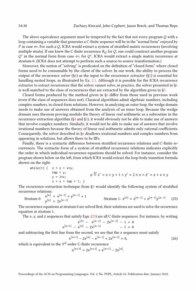
54:30 Zachary Kincaid, John Cyphert, Jason Breck, and Thomas Reps
The above equivalence argument must be tempered by the fact that not every program Q with a
loop containing a variable that generates a C-finite sequence will be in the “normal form” enjoyed by
P in case⇐. For such a Q , ICRA would extract a system of stratified matrix recurrences (involving
multiple strata). If one knew the C-finite recurrence RQ forQ , one could construct another program
Q ′ in the normal form from case ⇐; for Q ′, ICRA would extract a single matrix recurrence at
stratum-0. (ICRA does not attempt to perform such a source-to-source transformation.)
Moreover, the notion of “solving” is predicated on the definition of “closed form,” where closed
forms need to be consumable by the client of the solver. In our work, the ability to process the
output of the recurrence solver (§6) as the input to the recurrence extractor (§5) is essential forhandling nested loops, as illustrated by Ex. 2.1. Although it is possible for the ICRA recurrence
extractor to extract recurrences that the solver cannot solve, in practice, the solver presented in §6
is well-matched to the class of recurrences that are extracted by the algorithm given in §5.
Closed forms produced by the method given in §6 differ from those used in previous work
(even if the class of sequences does not). Classical algorithms admit algebraic numbers, including
complex numbers, in closed-form solutions. However, in analyzing an outer loop, the wedge domain
needs to make use of answers obtained from the analysis of an inner loop. Because the wedge
domain uses theorem proving modulo the theory of linear real arithmetic as a subroutine in the
recurrence-extraction algorithm (§4 and §5), it would obviously not be able to make use of answers
that involve complex numbers. Similarly, it would not be able to make use of answers that involve
irrational numbers because the theory of linear real arithmetic admits only rational coefficients.
Consequently, the solver described in §6 disallows irrational numbers and complex numbers from
appearing in solutions, but allows there to be IIFs.
Finally, there is a syntactic difference between stratified recurrence relations and C-finite re-
currences. The syntactic form of a system of stratified recurrence relations indicates explicitly
the order in which individual recurrence equations should be solved. For instance, consider the
program shown below on the left, from which ICRA would extract the loop-body transition formula
shown on the right.
while(*) { z = z + x*y;tmp = y;y = 2*x;x = x + tmp + 1; }
φdef
= x′ = x + y + 1 ∧ y′ = 2 × x ∧ z′ = z + x × y
The recurrence-extraction technique from §5 would identify the following system of stratified
recurrence relations:
Stratum 0:
x[n] = x[n−1] + y[n−1] + 1y[n] = 2x[n−1]
Stratum 1: z[n] = z[n−1] + x[n−1]y[n−1] (25)
The recurrence equations at stratum 0 are solved first; their solutions are used to solve the recurrence
equation at stratum 1.
The x, y, and z sequences that satisfy Eqn. (25) are all C-finite sequences. For instance, by writing
x[n] − x[n−1] − 2x[n−2] − 1 = 0
x[n+1] − x[n] − 2x[n−1] − 1 = 0
and subtracting the first line from the second, we see that the x sequence must satisfy
x[n+1] − 2x[n] − x[n−1] + 2x[n−2] = 0, (26)
which is equivalent to the 3rd-order C-finite recurrence
x[n+3] = 2x[n+2] + x[n+1] − 2x[n].
Proceedings of the ACM on Programming Languages, Vol. 2, No. POPL, Article 54. Publication date: January 2018.
Non-linear Reasoning for Invariant Synthesis 54:31
The recurrence equation for z, at stratum 1, is syntactically not a C-finite recurrence because it
contains the non-linear term x[n−1]y[n−1]. 6
The syntactic distinction between stratified recurrence relations and C-finite recurrences is
important from the viewpoint of recurrence extraction. In particular, the loop-body formula φ does
not entail Eqn. (26): x[n+1] and x[n−2] do not belong to the vocabulary of φ (which refers to only
two copies of x—one in the pre-state and one in the post-state).
Generating Functions. Operational calculus is a transform method: a recurrence relation is converted
into an algebraic problem; the algebraic problem is solved by algebraic manipulations; a solution in
ordinary algebra is read out of the solution to the algebraic problem. Generating functions [Wilf
1994] are another transform method that can be used to solve recurrence relations [Flajolet and
Sedgewick 2009]. With generating functions, a sequence a = ⟨a0,a1,a2, . . .⟩ is represented by the
sum (or power series)
∑∞n=0 anx
n. Multiplication of two sequences is performed as the following
convolution:
∑∞n=0 anx
n ∗∑∞
n=0 bnxn =
∑∞n=0
(∑ni=0 aibn−i
)xn . Thus, the multiplication operator
for generating functions is a convolution, whereas the multiplication in operational calculus is a
convolution difference (cf. Eqn. (4)).
Operational calculus and generating functions create different terms for subsequent algebraic
manipulation. Simpler terms might lead to a faster and simpler solver. However, as shown by the
following examples, neither technique can be said to have an advantage in this respect:
Operational calculus creates simpler terms: In operational calculus, the constant sequence λn.cis represented by c = ⟨c, c, . . .⟩, whereas the generating function is
c1−x . The respective values
for the sequence λn.n2 are 2
(q−1)2 +1
q−1 andx (x+1)(1−x )3 .
Generating functions create simpler terms: The generating function for the geometric sequence
λn.αn is1
1−αx , whereas the operational-calculus value isq−1q−α .
Operational calculus and generating functions create terms of similar complexity: The left-shift
operators are q and1
x , respectively; the right-shift operators are v and x , respectively.
Operational Calculus. We are not aware of other work that solves recurrences automatically using
operational calculus; Berg [1967] discusses recurrence solving in the style of a mathematics textbook,
but provides no explicit algorithm. §6.2 describes our mechanization of Berg’s approach. §6.3
concerns an extension to operational calculus not found in Berg (or elsewhere, as far as we know).
ACKNOWLEDGMENTSWe thank the anonymous reviewers and shepherd A. Rybalchenko for their comments on the
submission. This work was supported in part by a gift from Rajiv and Ritu Batra; by AFRL under
DARPA MUSE award FA8750-14-2-0270 and DARPA STAC award FA8750-15-C-0082; and by the
UW-Madison Office of the Vice Chancellor for Research and Graduate Education with funding
from WARF. Opinions, findings, conclusions, or recommendations expressed herein are those of
the authors and do not necessarily reflect the views of the sponsoring agencies.
REFERENCESE. Albert, P. Arenas, S. Genaim, and G. Puebla. 2008. Automatic Inference of Upper Bounds for Recurrence Relations in Cost
Analysis. In SAS. 221–237.E. Albert, S. Genaim, and A.N. Masud. 2013. On the inference of resource usage upper, lower bounds. Trans. on Computational
Logic 14, 3 (2013).Z. Ammarguellat and W. L. Harrison, III. 1990. Automatic recognition of induction variables and recurrence relations by
abstract interpretation. In PLDI. 283–295.
6A C-finite recurrence can contain only linear terms; however, a C-finite sequence may satisfy a recurrence relation that
contains a non-linear term.
Proceedings of the ACM on Programming Languages, Vol. 2, No. POPL, Article 54. Publication date: January 2018.
54:32 Zachary Kincaid, John Cyphert, Jason Breck, and Thomas Reps
C. Ancourt, F. Coelho, and F. Irigoin. 2010. A Modular Static Analysis Approach to Affine Loop Invariants Detection.
Electron. Notes Theor. Comput. Sci. 267, 1 (Oct. 2010), 3–16.T. Antonopoulos, P. Gazzillo, M. Hicks, E. Koskinen, T. Terauchi, and S. Wei. 2017. Decomposition Instead of Self-composition
for Proving the Absence of Timing Channels. In PLDI.R. Bagnara, A. Pescetti, A. Zaccagnini, and E. Zaffanella. 2005a. PURRS: Towards Computer Algebra Support for Fully
Automatic Worst-Case Complexity Analysis. CoRR abs/cs/0512056 (2005).
R. Bagnara, E. Rodríguez-Carbonell, and E. Zaffanella. 2005b. Generation of Basic Semi-Algebraic Invariants Using Convex
Polyhedra. In SAS.G. Barthe, J. Crespo, and C. Kunz. 2011. Relational Verification Using Product Programs. In Proceedings of the 17th International
Conference on Formal Methods (FM).G. Barthe, P.R. D’Argenio, and T. Rezk. 2004. Secure Information Flow by Self-Composition. In Comp. Sec. Found. Workshop.L. Berg. 1967. Introduction to the Operational Calculus. North-Holland Publishing Co., Amsterdam.
D. Beyer and M.E. Keremoglu. 2011. CPAchecker: A Tool for Configurable Software Verification. In CAV.R. Blanc, T. A. Henzinger, T. Hottelier, and L. Kovács. 2010. ABC: Algebraic Bound Computation for Loops. In Int. Conf. on
Logic for Programming, Art. Intell., and Reasoning. 103–118.B. Boigelot and P. Wolper. 1994. Symbolic verification with periodic sets. In CAV. 55–67.M. Bozga, R. Iosif, and F. Konečný. 2010. Fast Acceleration of Ultimately Periodic Relations. In CAV. 227–242.M. Brockschmidt, F. Emmes, S. Falke, C. Fuhs, and J. Giesl. 2014. Alternating runtime and size complexity analysis of integer
programs. In TACAS.B. Buchberger. 1976. A Theoretical Basis for the Reduction of Polynomials to Canonical Forms. SIGSAM Bull. 10, 3 (Aug.
1976), 19–29.
B.-Y.E. Chang and K.R.M Leino. 2005. Abstract Interpretation with Alien Expressions and Heap Structures. In VMCAI.J. S. Cohen. 2003. Computer Algebra and Symbolic Computation: Mathematical Methods. A K Peters/CRC Press.
M. A. Colón. 2004. Approximating the Algebraic Relational Semantics of Imperative Programs. In SAS. 296–311.P. Cousot and R. Cousot. 1979. Systematic Design of Program Analysis Frameworks. In POPL. 269–282.P. Cousot and N. Halbwachs. 1978. Automatic Discovery of Linear Constraints Among Variables of a Program. In POPL.D. A. Cox, J. Little, and D. O’Shea. 2015. Ideals, Varieties, and Algorithms: An Introduction to Computational Algebraic
Geometry and Commutative Algebra (4th ed.). Springer Publishing Company, Incorporated.
L. de Moura and N. Bjørner. 2008. Z3: An Efficient SMT Solver. In TACAS.S. de Oliveira, S. Bensalem, and V. Prevosto. 2016. Polynomial Invariants by Linear Algebra. In ATVA.I. Dillig, T. Dillig, B. Li, and K. McMillan. 2013. Inductive Invariant Generation via Abductive Inference. In OOPSLA.J. Esparza, S. Kiefer, and M. Luttenberger. 2010. Newtonian Program Analysis. J. ACM 57, 6 (2010).
A. Farzan and Z. Kincaid. 2015. Compositional Recurrence Analysis. In FMCAD.A. Finkel and J. Leroux. 2002. How to Compose Presburger-Accelerations: Applications to Broadcast Protocols. In FST TCS.
145–156.
P. Flajolet and R. Sedgewick. 2009. Analytic Combinatorics. Cambridge University Press.
pdfs.semanticscholar.org/d347/dbb4b2eea7fca0183b55112b9cc07faa51ff.pdf.
A. Flores-Montoya and R. Hähnle. 2014. Resource analysis of complex programs with cost equations. In APLAS.G. Gange, J. A. Navas, P. Schachte, H. Søndergaard, and P. J. Stuckey. 2016. An Abstract Domain of Uninterpreted Functions.
In VMCAI.P. Granger. 1992. Improving the Results of Static Analyses Programs by Local Decreasing Iteration. In FSTTCS.B.S. Gulavani and S. Gulwani. 2008. A Numerical Abstract Domain Based on Expression Abstraction and Max Operator
with Application in Timing Analysis. In CAV.S. Gulwani, A. Tiwari, and G.C. Necula. 2004. Join Algorithms for the Theory of Uninterpreted Functions. In FSTTCS.A. Gurfinkel, T. Kahsai, A. Komuravelli, and J.A. Navas. 2015. The SeaHorn Verification Framework. In CAV.M. Heizmann, J. Christ, D. Dietsch, E. Ermis, J. Hoenicke, M. Lindenmann, A. Nutz, C. Schilling, and A. Podelski. 2013.
Ultimate Automizer with SMTInterpol (Competition Contribution). In TACAS.A. Humenberger, M. Jaroschek, and L. Kovacs. 2017. Automated Generation of Non-Linear Loop Invariants Utilizing
Hypergeometric Sequences. In ISSAC.J.-G.-M. 1983. Hypernumbers. I. Algebra. Studia Math. 77 (1983), 3–16. matwbn.icm.edu.pl/ksiazki/sm/sm77/sm7712.pdf
Originally published in Polish in 1944.
B. Jeannet and A. Miné. 2009. Apron: A Library of Numerical Abstract Domains for Static Analysis. In CAV.B. Jeannet, P. Schrammel, and S. Sankaranarayanan. 2014. Abstract Acceleration of General Linear Loops. In POPL. 529–540.M. Kauers and P. Paule. 2011. The Concrete Tetrahedron. SpringerWienNewYork.
Z. Kincaid, J. Breck, A. Forouhi Boroujeni, and T. Reps. 2017. Compositional Recurrence Analysis Revisited. In PLDI.L. Kovács. 2008. Reasoning Algebraically About P-Solvable Loops. In TACAS.A. Miné. 2001. The Octagon Abstract Domain. In Working Conf. on Rev. Eng. 310–322.
Proceedings of the ACM on Programming Languages, Vol. 2, No. POPL, Article 54. Publication date: January 2018.
Non-linear Reasoning for Invariant Synthesis 54:33
M. Müller-Olm and H. Seidl. 2004. Precise Interprocedural Analysis through Linear Algebra. In POPL.T. Reps, M. Sagiv, and G. Yorsh. 2004. Symbolic Implementation of the Best Transformer. In VMCAI. 252–266.T. Reps and A. Thakur. 2016. Automating Abstract Interpretation. In VMCAI.T. Reps, E. Turetsky, and P. Prabhu. 2016. Newtonian Program Analysis via Tensor Product. In POPL.E. Rodríguez-Carbonell and D. Kapur. 2004. Automatic Generation of Polynomial Loop Invariants: Algebraic Foundations.
In ISSAC. 266–273.S. Sankaranarayanan, H.B. Sipma, and Z. Manna. 2004. Non-Linear Loop Invariant Generation using Gröbner Bases. In
POPL.A. Srikanth, B. Sahin, and W.R. Harris. 2017. Complexity Verification Using Guided Theorem Enumeration. In POPL.T. Terauchi and A. Aiken. 2005. Secure Information Flow As a Safety Problem. In Static Analysis Symp.A. Thakur. 2014. Symbolic Abstraction: Algorithms and Applications. Ph.D. Dissertation. Comp. Sci. Dept., Univ. of Wisconsin,
Madison, WI. Tech. Rep. 1812.
A. Thakur and T. Reps. 2012. A Method for Symbolic Computation of Abstract Operations. In CAV.H. Wilf. 1994. Generatingfunctionology, 2nd. Ed. Academic Press. www.math.upenn.edu/ wilf/gfologyLinked2.pdf.
Proceedings of the ACM on Programming Languages, Vol. 2, No. POPL, Article 54. Publication date: January 2018.