non-linear, non-parametric, non-fundamental exchange rate forecasting

Copyright © 2006 John Wiley & Sons, Ltd.

Non-linear, Non-parametric, Non-fundamental Exchange Rate Forecasting

NIKOLA GRADOJEVIC1* AND JING YANG2†

1 Faculty of Business Administration, Lakehead University,Thunder Bay, Ontario, Canada2 Financial Markets Department, Bank of Canada, Ottawa,Ontario, Canada

ABSTRACTThis paper employs a non-parametric method to forecast high-frequency Canadian/US dollar exchange rate. The introduction of a microstructure variable, order flow, substantially improves the predictive power of both linearand non-linear models. The non-linear models outperform random walk andlinear models based on a number of recursive out-of-sample forecasts. Twomain criteria that are applied to evaluate model performance are root meansquared error (RMSE) and the ability to predict the direction of exchange ratemoves. The artificial neural network (ANN) model is consistently better inRMSE to random walk and linear models for the various out-of-sample setsizes. Moreover, ANN performs better than other models in terms of percent-age of correctly predicted exchange rate changes. The empirical results suggestthat optimal ANN architecture is superior to random walk and any linear com-peting model for high-frequency exchange rate forecasting. Copyright ©2006 John Wiley & Sons, Ltd.

key words market microstructure; artificial neural networks; foreignexchange rate forecasting

INTRODUCTION

Understanding exchange rate movements has long been an extremely challenging and important taskfor academic and business researchers. Not only is the exchange rate a significant determinant ofaggregate demand in a small open economy such as Canada’s, but it also responds immediately andmaterially to monetary policy. However, the response is not always predictable. This makes it some-times difficult to achieve the desired results of monetary policy implementation.

Efforts to deepen our understanding of exchange rate movements have taken on a number ofapproaches. Initially, efforts centered on the development of low-frequency macroeconomic (fun-damental) empirical models. More recently, efforts have been aimed at the development of high-

Journal of ForecastingJ. Forecast. 25, 227–245 (2006)Published online 27 February 2006 in Wiley InterScience(www.interscience.wiley.com) DOI: 10.1002/for.986

* Correspondence to: Nikola Gradojevic, Faculty of Business Administration, Lakehead University, 955 Oliver Road,Thunder Bay, Ontario P7B 5E1, Canada. E-mail: [email protected]† Current address: International Finance Division, Bank Of England, London, UK. The views expressed in this paper arethose of the authors and do not reflect those of the Bank of Canada or the Bank of England.

228 N. Gradojevic and J. Yang

Copyright © 2006 John Wiley & Sons, Ltd. J. Forecast. 25, 227–245 (2006)DOI: 10.1002/for

frequency models of the foreign exchange (FX) market, based on microeconomic (microstructure)variables. Throughout, however, forecasting models have been developed for obvious utilitarian pur-poses, but they have also served as a gauge of our understanding of exchange rate movements. More-over, they can sometimes help to pinpoint where the gaps in our knowledge may lie, and thereforesuggest new avenues of research. The exchange rate forecasting model developed in this paper servesall of these purposes.

Given the failure of traditional FX rate models to explain and predict exchange rate fluctuationscorrectly (Meese and Rogoff, 1983), we turn to the market microstructure of FX markets. In recentyears there has been a lot of evidence that the behavior of dealers and other market participants caninfluence equilibrium exchange rates (Lyons and Evans, 2002; Covrig and Melvin, 1998). Inventoryadjustments and bid–ask spread reactions to informative incoming order flows are two examples inwhich dealer behavior affects exchange rate determination. Indeed, given that different market participants trade based on private as well as public information sets, it is natural to assume thatequilibrium exchange rate expectations are formed based on a combination of macroeconomic fundamentals and market microstructure variables (Goldberg and Tenorio, 1997). Moreover, it ismost likely that the macroeconomic information and order flow information are processed in a non-linear fashion.

This paper contributes to the FX forecasting literature in the following aspects. First, we extendthe empirical macroeconomic FX models to include ‘non-fundamental’ variables such as order flow.Second, we employ a non-parametric method, artificial neural network (ANN), to capture the non-linear relationship between exchange rate and the informational content of trades and public infor-mation. Our study shows that non-linearities and order flows information play important roles forexchange rate determination and very short-term forecasting. In particular, the inclusion of addi-tional microstructure variables and ANNs results in out-of-sample forecasts superior to those fromrandom walk and linear models for daily Canadian/US dollar exchange rate movements. Three sta-tistics are used to compare models: root-mean squared error (RMSE), mean squared prediction error(MSPE) and the percentage of correctly predicted exchange rate changes (PERC). Empirical find-ings are in favor of the ANN model, which yields a very robust out-of-sample forecasting improve-ment in RMSE, MSPE and PERC.

Our results generate important empirical and theoretical implications. Prior to this work, ANN exchange rate models were built mostly on macroeconomic, technical trading or autoregres-sive foundations (Gencay, 1999; Kuan and Liu, 1995; Plasmans et al., 1998) and the evidence from them was mixed. Our study suggests the importance of market microstructure variables in FXdetermination.

Moreover, we point to important implications beyond those given by Lyons and Evans (2002) andLyons (2001). What makes their dynamic, temporary equilibrium structure relatively easy to char-acterize is its linear structure. However, we find that market participants (i.e., dealers) are likely topursue more complex or even mixed strategies. This brings us to the notion of a non-linear equilib-rium where market makers create a non-linear relation between public information, microstructureeffects and exchange rates. One of the major strengths of this work is its strong empirical evidencethat requires expansion of traditional microstructure linear characterization of equilibria as well asfundamental models of FX markets. We attempt to describe this new model only to a limited extentand more extensive research is required. In light of these findings, we challenge theoreticalresearchers to derive and explain this non-linear microstructure model more formally.

The next section describes the competing theoretical models. The third section offers a short dis-cussion on backpropagation ANNs. The fourth section describes the data and the method used to

Non-linear Exchange Rate Forecasting 229


assess the predictive performance of the models. The fifth section describes the empirical results ofthe models. The final section concludes the paper and recommends further research.

MODELS OF EXCHANGE RATE DETERMINATION

Various models aiming at explaining exchange rate fluctuations have been proposed. Meese andRogoff (1983) found that a simple random walk model performed no worse than any of competingrepresentative time series and structural exchange rate models. Out-of-sample forecasting power inthose models was surprisingly low for various forecasting horizons (from 1 to 12 months).

Subsequent attempts to determine exchange rates shed very little light on the problem. Baillie andMcMahon (1989) pointed out that exchange rates are in general not linearly predictable. They aredescribed as highly volatile with an elusive data-generating process (DGP). Similarly, Hsieh (1988),Boothe and Glassman (1987) and Diebold and Nerlove (1989) observed that exchange rate changesare leptokurtic and may be non-linearly dependent. Further, the observed exchange rates seem toexhibit volatility clustering, i.e., high (low) volatility periods tend to be followed by high (low)volatile periods. This conditional heteroskedasticity evidence was reported in Hsieh (1989) and Engleet al. (1990). Nevertheless, excess kurtosis and conditional heteroskedasticity in the residuals maynot improve point forecasts because these effects operate through even-ordered moments. To modelthe observed effects, parametric non-linear models such as ARCH (Hsieh, 1989) and GARCH(Bollerslev, 1990) were applied to exchange rates modeling, but with very little success. Gencay(1999) examined the predictability of spot foreign exchange rate returns using moving average tech-nical trading rules and GARCH, nearest neighbors (NN) and ANN models. GARCH models gener-ated insignificant sign forecasts improvement (and less than 1% mean-squared error improvement)over a simple random walk. As noted in Diebold and Nason (1990), the pre-specification of theGARCH model form may neglect other possible non-linearities resulting from a true DGP. Meeseand Rose (1991) examined macroeconomic exchange rate models and found that poor explanatorypower of the models cannot be attributed to non-linearities. They considered five non-linear struc-tural exchange rate models in order to capture possible non-linearities. The application of severalparametric and non-parametric techniques on these fundamentally driven models did not show anyimprovement in our ability to understand the exchange rate fluctuations.

Meese and Rose (1990) and Diebold and Nason (1990) used an NN non-parametric method calledlocally weighted regression to estimate non-linearities in exchange rates. As a result, Meese andRose (1990) rejected the existence of non-linearities. Diebold and Nason (1990) could not signifi-cantly improve upon a simple random walk in the out-of-sample exchange rate predictions. In con-trast, using an NN method, Gencay (1999) and Lisi and Medio (1997) were able to generatepredictions superior to those generated by the random walk model. This mixed evidence couldsuggest an existence of non-linear patterns in the exchange rates which, if revealed, could beexploited to improve both point and sign predictions.

Kuan and Liu (1995) used backpropagation and recurrent ANNs, a very powerful tool for detect-ing non-linear patterns, to investigate the ANN’s out-of-sample forecasting ability on five exchangerates (British pound, Canadian dollar, Deutschemark, Japanese yen, and Swiss franc) against the USdollar. The data were daily opening bid prices of the NY Foreign Exchange Market and the modelof interest was a non-linear autoregressive model where its performance against random walk andARMA processes was measured. Their results showed the presence of non-linearities in exchangerates time series. For the Japanese yen and British pound, ANNs exhibited significant sign predic-



tions and/or significantly lower out-of-sample MSPE (relative to the random walk model); for theremaining three currencies ANNs had inferior forecasting performance. Some other studies involv-ing ANNs were less encouraging. Plasmans et al. (1998) and Verkooijen (1996) used macroeco-nomic models, but they could not produce any satisfactory monthly forecasts. However, Zhang andHu (1998) modeled exchange rate as depending non-linearly on its past values, and their model out-performed simple linear models, but they never compared it to a random walk. Hu et al. (1999)showed (using daily and weekly data) that ANNs are a more robust forecasting method than a randomwalk model. Hence, the application of ANNs to short-term currency behavior was successful innumerous cases and the results suggest that ANN models may have some advantages when frequentshort-term forecasts are required.1

All the above-mentioned approaches try to find the exchange rate determinants among macro-economic variables such as interest rates, money supplies, inflation rates, and trade balances. Floodand Rose (1995) concluded that exchange rate modeling based only on macroeconomic fundamen-tals might be insufficient to explain exchange rate volatility. Recently, Cheung and Wong (2000)conducted a survey of practitioners in the interbank foreign exchange markets in Hong Kong, Tokyoand Singapore. A majority of participants view short-term exchange rate variability closely relatedto non-economic forces including bandwagon effects, overreaction to news, speculation and techni-cal trading. Only 1% of the traders look at economic fundamentals to determine daily exchange ratemovements.

Given the partial empirical success of the macroeconomic models, there is an increasing interestin the exchange rate microstructure. The microstructure approach investigates how specific tradingmechanisms affect the exchange rate formation. Lyons and Evans (2002) incorporated a variablereflecting the microeconomics of asset pricing into a model of the exchange rate. They introducedthe most important microstructure variable, ‘order flow’, as the proximate determinant of theexchange rate (using daily data over a 4-month period) and were able to significantly improve onexisting macroeconomic models. More precisely, they managed to capture about 60% of theexchange rate daily changes using a linear model.

In general, there are two broad theories of exchange rate modeling: traditional macroeconomicmodels and the more recently developed market microstructure models. Macroeconomic models aimat modeling and estimating exchange rates at monthly or lower frequency. These models are ingeneral of the following form:

(1)

where Drpfxt is the change in the logarithm of the real exchange rate over the month or some lowerfrequency of observations, and Mt is a vector of typical macroeconomic variables such as the dif-ference between home and foreign nominal interest rates, the long-run expected inflation differen-tial and relative real growth rates.2 To control for the key Canadian macroeconomic variables, thispaper uses a variation of the model developed by Amano and van Norden (1995):

(2)Drpfx rpfx com ene intdifft t t t t t t N= ( ) + =f d, , , , , . . . ,1

Drpfx Mt t t t N= ( ) + =f e , , . . . ,1

1 In this context, ANNs focus on daily (weekly) or less-than-a monthly forecasting frequency, while typical macroeconomicmodels are at a monthly or quarterly frequency.2 See Meese and Rogoff (1983).



where rpfxt is real Canadian/US exchange rate deflated by GDP deflators, comt is the logarithm ofnon-energy commodity price index (deflated by the US GDP deflator), enet is the logarithm of energycommodity price index (deflated by the US GDP deflator) and intdifft represents the nominal 90-daycommercial paper interest rate differential (Canada–USA).

Macroeconomic models provide no role for any ‘market microstructure’ effects to directly enterinto the estimated equation which are thus incorporated through the error term dt.3 These modelsassume that markets are efficient in the sense that information is widely available to all market par-ticipants and all relevant and ascertainable information is already reflected in exchange rates. In otherwords, from this point of view, exchange rate changes are not informed by microstructure variables.However, typical macroeconomic models perform poorly. Moreover, empirical evidence from Lyonsand Evans (2002), Covrig and Melvin (1998) and this paper suggests that a microstructure variable‘order flow’ contains information relevant to exchange rate determination.4

For the spot FX trader, what really matters is not the data on any of the macroeconomic funda-mentals, but information about demand for currencies extracted from purchases and sales orders, ororder flow (Cheung and Wong, 2000). Any short-term exchange rate determinant such as portfolioshifts, overreaction to news or speculative trading would be recorded in order flow. It is presumedthat certain FX traders observe trades that are not observable to all the other traders and, in turn, themarket efficiency assumption is violated at least in the very short term.5

Microstructure models directly rely on information regarding the order flow. Lyons and Evans(2002) approach an order flow/exchange rate relation through a very realistic framework–portfolioshifts model. They use the perfect Bayesian–Nash equilibrium and explicitly derive an equilibriumprice change (between period t - 1 and t) and equilibrium trading strategies. Intuitively, equilibriumprice is determined from the common information set (macroeconomic fundamentals, denoted rt)and aggregate interdealer order flow (denoted IBt):

(3)

where l is a positive constant.This model was estimated over a 4-month span of daily observations controlling for a key macro-

economic variable: interest rate differential. The results were in favor of a microstructure approachwith an R2 statistic over 50%.

However, there are several unanswered questions which require further research. First, can thismodel be used for out-of-sample forecasting? Lyons and Evans (2002) model is based on realizedorder flow information which is not available ex ante.6 Secondly, is there a non-linear conditionalmean function that characterizes a true DGP? By employing ANNs and relaxing the restrictions ofthe model by Lyons and Evans (2002), we attempt to find another equilibrium, non-linear by its

DP IBt t tr= + l

3 Microstructure literature examines the elements of the security trading process: the arrival and dissemination of informa-tion; the generation and arrival of orders; and the market architecture which determines how orders are transformed intotrades. Prices are discovered in the marketplace by the interaction of market design and participant behavior.4 Order flow is explained in the next section.5 It may be that markets, absent these market microstructure frictions, would be efficient, but trading frictions impede theinstantaneous embodiment of all information into prices.6 We also experimented with the linear regression and realized order flow information as explanatory variables and obtainedthe R2 statistic around 40%. However, we choose to use lagged order flow variables throughout the study since the same-period order flow information is not available ex ante and therefore it can not be used in a forecasting model.



structure.7 Indeed, in this new setting there is a possibility that other types of order flow might playa role in setting the price. Finally, can we restrict our model to only one macroeconomic determi-nant? In this paper, we try to control (among other candidates available on a daily basis) for anotherfundamental variable: crude oil price. We address all of these issues and provide adequate answersbased solely on empirical grounds.

In general, the market microstructure approach assumes the following relationship between theexchange rate and the driving variables:

(4)

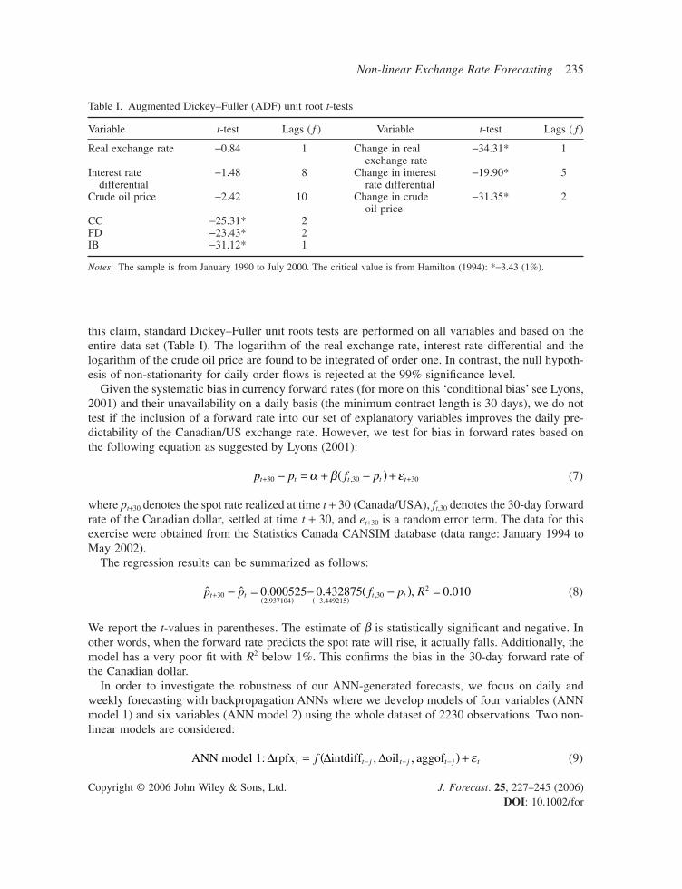
where Dxt represents order flow, DIt is a change in net dealer positions, while Nt is any other micro-economic variable. Order flow can be positive (net dollar purchases), or negative (net dollar sales).Macroeconomic effects are incorporated into an error term Xt. A positive relationship between theexchange rate and order flow is expected since informational asymmetries gradually affect the priceuntil it reaches equilibrium. Figure 1 illustrates the explanatory power of an aggregate order flow andits IB component (the data cover the period from January 1990 to June 2000 at a daily frequency).

As the solid line indicates, the Canadian dollar has depreciated throughout most of the sample.The relationship between the exchange rate and order flow is quite clear as a positive correlation

D D Drpfx I Nt t t t tx t N= ( ) + =y , , , , . . . ,X 1

7 For example, Bhattacharya and Spiegel (1991) and Rochet and Vila (1994) show that microstructure models can have multiple or non-linear equilibria. Lyons and Evans (2002) add a squared order flow term into their regression, but find itinsignificant.

0 500 1000 1500 2000 2500-1

-0.5

0

0.5

1

Observation number

March 5th, 1990

June 30th, 2000

Cumulative aggregate order flow Log real exchange rate

0 10 20 30 40 50 600.5

0.55

0.6

0.65

0.7

0.75

Observation number

December, 1999February, 2000

Cumulative IB order flow Log real exchange rate

Figure 1. Above: Aggregate (cumulative) order flow and log Canadian/US real exchange rate. Below: IB(cumulative) order flow and log Canadian/US real exchange rate. Note: All values are normalized to [-1, 1]



between cumulative purchases of US dollars and the depreciation. This relationship is more obviousfrom the 3-month sample (December 1999 to February 2000) of IB order flow and log Canadian/USreal exchange rate. However, it would be inappropriate to assume that order flow contains all theinformation that is relevant for exchange rates.

This paper combines macroeconomic and microstructure approaches into a single high-frequencydata model.8 More specifically, it embodies modified models from Amano and van Norden (1995,1998) and Lyons and Evans (2002):

(5)

where Dintdifft is the change in the differential between the Canadian and US nominal 90-day com-mercial paper rates, Doilt is the daily change in the logarithm of the crude oil price, and order flowis denoted by Dxt. Later in the paper, Dxt is substituted by either a vector of three different order flowtypes or aggregate order flow. ANNs are employed to estimate a non-linear relationship betweenexchange rate movements and these variables.

BACKPROPAGATION ANNS

The backpropagation ANN, a network type applied in this paper, is probably the most commonlyused ANN. Backpropagation learning algorithm requires continuous differentiable non-linearitiesand the most commonly used type is the sigmoid logistic (or logsig) function:9

(6)

Studies by Cybenko (1989) and Funahashi (1989) show that the backpropagation non-linear repre-sentation with sigmoid non-linearities can approximate a large number of mappings between inputsand outputs reasonably well. This makes ANN a very useful non-parametric technique and there isno need for any unjustified restrictions often present in econometric modeling.

Backpropagation estimation techniques are important for large samples and real-time applicationssince they allow for adaptive estimation. However, they may not fully utilize the information in thedata. White (1989) showed that the recursive estimator is not as efficient as the non-linear leastsquares estimator. An important aspect of the backpropagation methods is the choice of the learn-ing rate h. The inefficiency of the backpropagation originates in keeping the learning rate constantin an environment where the influence of random movements in inputs is not accounted by the target.This would lead the parameter vector to fluctuate indefinitely, i.e., there would be no convergence.A minimum requirement is to gradually drive the learning rate to zero to achieve convergence. Infact, White (1989) demonstrated that ht has to be chosen not as a vanishing scalar, but as a gradu-ally vanishing matrix of a very specific form. These arguments on learning rates are only valid ifthe environment is stationary, which is the case in this work (as well as the constant learning rate).

f we w

( ) =+ -

1

1

D Y D D Drpfx intdiff oilt t t t tx t N= ( ) + =- - -1 1 1 1, , , , . . . ,h

8 For example, Goldberg and Tenorio (1997) and Osler (1998) also follow this approach.

9 Other types of transfer functions used in this research are tan–sigmoid and purelin ( f(w) = w).f we e

e e

w w

w w( ) = -

+ÊËÁ

ˆ¯̃

-

-



However, instead of tuning the network’s learning rate, we attempt to balance the bias and varianceand avoid non-convergence with early stopping. This may slightly deteriorate the model’s perform-ance and we acknowledge that probably by following White (1989) an optimal estimator would beachieved.

MODEL SPECIFICATION

Data descriptionThe order flow data were obtained from the Bank of Canada’s unique Daily Foreign ExchangeVolume Report, which is coordinated by the bank and organized through the Canadian ForeignExchange Committee (CFEC). Details about the trading flows (in Canadian dollars) for six majorCanadian commercial banks are categorized by the type of trade (spot, forward, and futures) andtransaction type (i.e., with regard to trading partner).10 Because this paper focuses on a short-termexchange rate forecast, spot transactions are of interest. In a spot transaction, a currency is tradedfor immediate delivery and payment is made within two business days of the contract entry date.Spot transactions vary, as follows:

• Commercial client transactions (CC) include all transactions with resident and non-resident non-financial customers.

• Canadian-domiciled investment transactions (CD) include all transactions with non-dealer finan-cial institutions located in Canada.

• Foreign institution transactions (FD) include all transactions with foreign financial institutions,such as FX dealers.

• Interbank transactions (IB) include transactions with other chartered banks, credit unions, invest-ment dealers and trust companies in the interbank market.

Because it was unavailable prior to 1994, CD transactions are excluded as an explanatory variablein this work. Moreover, according to Reuters Dealing 2000–1 electronic dealing system, IB trans-actions account for about 75% of total trading in major spot markets (Lyons and Evans, 2002). Thus,the CD transactions contribution in daily exchange rate explanation is relatively small and our resultssupport this conjecture.

Individual order flows (CC, FD, IB) are measured as the difference between the number of cur-rency purchases (buyer-initiated trades) and sales (seller-initiated trades). Aggregate order flow(aggof) is the sum of individual order flows. As noted earlier, the other variables of interest are thecrude oil closing price (in US dollars) deflated by the US consumer price index (CPI) (Doil) and thechange in the difference between nominal 90-day commercial paper rates in Canada and the USA(Dintdiff). The dependent variable dataset comprises the logarithm of real Canadian/US exchangerate daily changes (Drpfx) between January 1990 and June 2000. The real exchange rate was cal-culated from the nominal exchange rate and CPI for the USA and Canada.

All variables are considered in first-difference terms, because the daily change (positive or nega-tive) prediction is of interest. Also, by using the first differences we avoid theoretical problems ofestimation of non-stationary non-parametric functions (see Diebold and Nerlove, 1990). To support

10 The six banks used in this research account for approximately 83% of all Canada/US dollar transactions. The remainingtransactions occur within Canada (4%) and in the USA and the rest of the world (13%). Source: Bank of Canada.



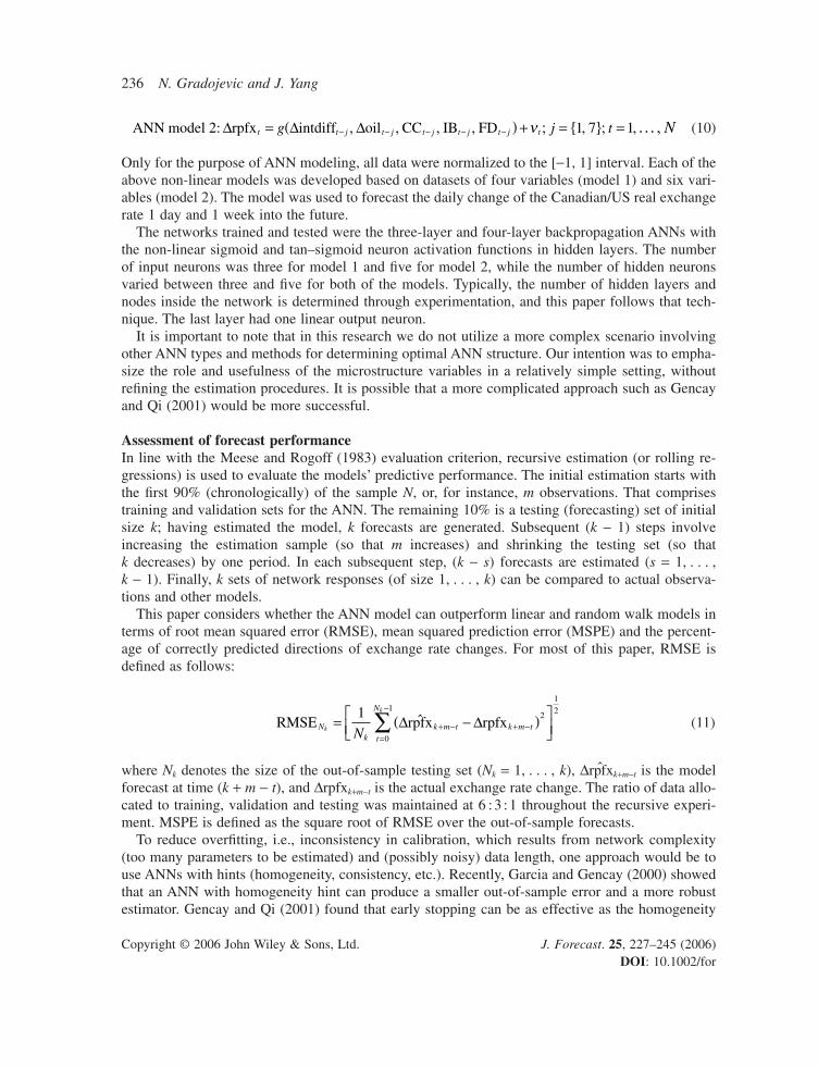
this claim, standard Dickey–Fuller unit roots tests are performed on all variables and based on theentire data set (Table I). The logarithm of the real exchange rate, interest rate differential and thelogarithm of the crude oil price are found to be integrated of order one. In contrast, the null hypoth-esis of non-stationarity for daily order flows is rejected at the 99% significance level.

Given the systematic bias in currency forward rates (for more on this ‘conditional bias’ see Lyons,2001) and their unavailability on a daily basis (the minimum contract length is 30 days), we do nottest if the inclusion of a forward rate into our set of explanatory variables improves the daily pre-dictability of the Canadian/US exchange rate. However, we test for bias in forward rates based onthe following equation as suggested by Lyons (2001):

(7)

where pt+30 denotes the spot rate realized at time t + 30 (Canada/USA), ft,30 denotes the 30-day forwardrate of the Canadian dollar, settled at time t + 30, and et+30 is a random error term. The data for thisexercise were obtained from the Statistics Canada CANSIM database (data range: January 1994 toMay 2002).

The regression results can be summarized as follows:

(8)

We report the t-values in parentheses. The estimate of b is statistically significant and negative. Inother words, when the forward rate predicts the spot rate will rise, it actually falls. Additionally, themodel has a very poor fit with R2 below 1%. This confirms the bias in the 30-day forward rate ofthe Canadian dollar.

In order to investigate the robustness of our ANN-generated forecasts, we focus on daily andweekly forecasting with backpropagation ANNs where we develop models of four variables (ANNmodel 1) and six variables (ANN model 2) using the whole dataset of 2230 observations. Two non-linear models are considered:

(9)ANN model 1: rpfx intdiff oil aggofD D Dt t j t j t j tf= ( ) +- - -, , e

ˆ ˆ . . , .. .

,p p f p Rt t t t+( ) -( )

- = - -( ) =302 937104 3 449215

3020 000525 0 432875 0 010

p p f pt t t t t+ +- = + -( ) +30 30 30a b e,

Table I. Augmented Dickey–Fuller (ADF) unit root t-tests

Variable t-test Lags ( f ) Variable t-test Lags ( f )

Real exchange rate -0.84 1 Change in real -34.31* 1exchange rate

Interest rate -1.48 8 Change in interest -19.90* 5differential rate differential

Crude oil price -2.42 10 Change in crude -31.35* 2oil price

CC -25.31* 2FD -23.43* 2IB -31.12* 1

Notes: The sample is from January 1990 to July 2000. The critical value is from Hamilton (1994): *-3.43 (1%).



(10)

Only for the purpose of ANN modeling, all data were normalized to the [-1, 1] interval. Each of theabove non-linear models was developed based on datasets of four variables (model 1) and six vari-ables (model 2). The model was used to forecast the daily change of the Canadian/US real exchangerate 1 day and 1 week into the future.

The networks trained and tested were the three-layer and four-layer backpropagation ANNs withthe non-linear sigmoid and tan–sigmoid neuron activation functions in hidden layers. The numberof input neurons was three for model 1 and five for model 2, while the number of hidden neuronsvaried between three and five for both of the models. Typically, the number of hidden layers andnodes inside the network is determined through experimentation, and this paper follows that tech-nique. The last layer had one linear output neuron.

It is important to note that in this research we do not utilize a more complex scenario involvingother ANN types and methods for determining optimal ANN structure. Our intention was to empha-size the role and usefulness of the microstructure variables in a relatively simple setting, withoutrefining the estimation procedures. It is possible that a more complicated approach such as Gencayand Qi (2001) would be more successful.

Assessment of forecast performanceIn line with the Meese and Rogoff (1983) evaluation criterion, recursive estimation (or rolling re-gressions) is used to evaluate the models’ predictive performance. The initial estimation starts withthe first 90% (chronologically) of the sample N, or, for instance, m observations. That comprisestraining and validation sets for the ANN. The remaining 10% is a testing (forecasting) set of initialsize k; having estimated the model, k forecasts are generated. Subsequent (k - 1) steps involveincreasing the estimation sample (so that m increases) and shrinking the testing set (so that k decreases) by one period. In each subsequent step, (k - s) forecasts are estimated (s = 1, . . . , k - 1). Finally, k sets of network responses (of size 1, . . . , k) can be compared to actual observa-tions and other models.

This paper considers whether the ANN model can outperform linear and random walk models interms of root mean squared error (RMSE), mean squared prediction error (MSPE) and the percent-age of correctly predicted directions of exchange rate changes. For most of this paper, RMSE isdefined as follows:

(11)

where Nk denotes the size of the out-of-sample testing set (Nk = 1, . . . , k), Drp̂fxk+m-t is the modelforecast at time (k + m - t), and Drpfxk+m-t is the actual exchange rate change. The ratio of data allo-cated to training, validation and testing was maintained at 6 :3 :1 throughout the recursive experi-ment. MSPE is defined as the square root of RMSE over the out-of-sample forecasts.

To reduce overfitting, i.e., inconsistency in calibration, which results from network complexity(too many parameters to be estimated) and (possibly noisy) data length, one approach would be touse ANNs with hints (homogeneity, consistency, etc.). Recently, Garcia and Gencay (2000) showedthat an ANN with homogeneity hint can produce a smaller out-of-sample error and a more robustestimator. Gencay and Qi (2001) found that early stopping can be as effective as the homogeneity

ˆRMSE rpfx rpfxNk

k m t k m t

t

N

k

k

N= -( )È

ÎÍ˘˚̇

+ - + -=

-

Â1 2

0

112

D D

ANN model 2: rpfx intdiff oil CC IB FDD D Dt t j t j t j t j t j tg j t N= ( ) + = { } =- - - - -, , , , ; , ; , . . . ,n 1 7 1



hint in pricing options. By using early stopping in this paper we assume that response functions areestimated consistently.

In addition to RMSE, the percentage of correctly predicted signs (PERC) of the forecast variableDrpfxt is considered; this is the total number of correctly forecast positive and negative movements,defined as

(12)

where

Sometimes, the significance of the difference in the performance of alternative models (dt) has to betested. We use the Diebold–Mariano test (Diebold and Mariano, 1995) to test the null hypothesisthat there is no difference in the MSPE and PERC of two alternative models (in our case of therandom walk and the ANN models).

The Diebold–Mariano test statistic for the equivalence of forecast errors is

(13)

where M is the testing set size and f(0) is the spectral density of dt at frequency zero. Diebold andMariano show that S1 is asymptotically distributed as a N(0, 1).

As forecasts are done only one step ahead we do not have to include any of the sample autoco-variances to calculate the long-run variance of dt, 2pf(0). In this case, a consistent estimate of 2pf(0)will be the sample variance of dt (see Diebold and Mariano, 1995).

EMPIRICAL RESULTS

We investigate the robustness of the forecasting performance of ANN models in this section. Thefollowing models are considered:

Random walk model (RW):

(14)

Linear model (LM1):

(15)

Linear model (LM2):

D D Drpfx intdiff oil IBt t j t j t j t t N= + + + + =- - -g g g g e0 1 2 3 1, , . . . ,

rpfx rpfxt t j t t N= + + =-a g0 1, , . . . ,

SM

d

fM

t

t

M

11

1

2 0=

[ ]

( )=

Âp

ptt t=◊( ) >ÏÌ

Ó1 0

0

if rpfx rpfx

otherwise

D D ,ˆ

PERC NN

pkk

t

t

M

( ) ==

Â1

1



(16)

ANN model 1:

(17)

ANN model 2:

(18)

j = {1, 7}, t = 1, . . . , N

Table II presents linear regression estimation results for these models based on the first 2005 obser-vations (initial estimation set). The impact of interest rate is more significant for j = 7, while the estimator of oil price is more significant for 1-day-ahead forecasting. Also, order flows are moreimportant for the shorter forecast horizon. Even though it is very small, as expected, the R2 increasedwhen individual order flows were taken into account.11

Two above-specified non-linear models (ANN 1 and ANN 2) were estimated by feedforward back-propagation ANNs. Overtraining was prevented by stopping the training process when the valida-tion set error started to increase.

D D Drpfx intdiff oil CC IB FDt t j t j t j t j t j tg t N= ( ) + =- - - - -, , , , , . . . ,, n 1

D Drpfx intdiff oil aggoft t j t j t j tf t N= ( ) + =- - -, , , , . . . ,e 1

D D Drpfx intdiff oil CC IB FDt t j t j t j t j t j t t N= + + + + + + =- - - - -b b b b b b n0 1 2 3 4 5 1, , . . . ,

Table II. Estimation results for linear models

Estimates (standard error) Model

Linear model 1 Linear model 1 Linear model 2 Linear model 2( j = 1) ( j = 7) ( j = 1) ( j = 7)

g0 (exp 10-5) 8.09 36.53(2.93e-05) (7.08e-05)

b0 (exp 10-5) 8.72 36.35(2.93e-05) (7.15e-05)

Dintdifft-j (exp 10-4) -1.13 -6.76 -1.89 -6.63(0.00025) (0.00026) (0.00025) (0.00026)

Doilt-j -0.0090 -0.003 -0.0087 -0.003(0.0065) (0.0073) (0.0065) (0.0073)

aggoft-j (exp 10-7) -1.35 -3.74(8.96e-08) (2.16e-07)

CCt-j (exp 10-7) 1.33 -4.55(1.28e-07) (3.11e-07)

IBt-j (exp 10-7) -1.015 -2.66(1.69e-07) (4.07e-07)

FDt-j (exp 10-7) -3.86 -3.78(8.98e-08) (2.16e-07)

R2 0.0021 0.005 0.0049 0.0055

11 This work uses daily data over a 10-year period (as opposed to the 4-month span used by Lyons and Evans, 2002); there-fore, the linear ‘microstructure’ model’s R2 is significantly lower.



Full sample estimation of 2230 observations was used to compare the ANN and linear models’performance. After the initial estimation of the models in the first 2005 observations, a set of out-of-sample forecasts was used to generate RMSEs. Each recursive re-estimation added 10 observa-tions, so that 18 RMSEs were calculated on out-of-sample datasets ranging in size from 225 to 55observations. This led to the selection of an ANN model 1 and ANN model 2 for 1-day-ahead ( j =1) and for 1-week-ahead ( j = 7) forecasts of exchange rate changes, which were compared to linearmodels 1 and 2 and the random walk model.

Tables III (for j = 1) and IV (for j = 7) list the RMSE statistics. They show that the ANN canproduce promising short-run forecasts, since the RMSE for the ANN model for a given forecastinghorizon is equal to or below both of the competing models.

The experiments show that the ANN model forecasts 1-day and 7-day-ahead exchange ratechanges better than the linear and random walk models. Nevertheless, the primary indicator of goodforecasting power is not necessarily RMSE, but the percentage of correctly forecast directions ofreal exchange rate fluctuations. In this case, the estimation involves very small values (exp 10-3) thatmight result in small RMSEs. In turn, the presence of small RMSEs is not a guarantee that the pre-diction is accurate, and caution is required when interpreting the estimation results.

As noted above, the percentage of correctly forecast exchange rate direction changes (PERC) isalso considered. Recursive regression for horizons between 5 and 225 observations (step 5) revealsthe superiority of the ANN model.12 ANN model 1 (2) correctly predicted, on average, 60.14%(61.81%) of the direction of daily exchange rate movements, while linear model 1 (2) correctly predicted 57.18% (58.75%) of such changes, and the random walk model predicted 54.88%. One-

Table III. RMSE (exp 10-3 ) for ANN, linear and random walk models ( j = 1)

Sample size Model

Random walk Linear model 1 ANN model 1 Linear model 2 ANN model 2( j = 1) ( j = 1) ( j = 1) ( j = 1) ( j = 1)

225 1.4321 1.4364 1.4270 1.4331 1.4216215 1.4168 1.4201 1.4121 1.4155 1.4060205 1.4232 1.4272 1.4163 1.4218 1.4119195 1.4216 1.4240 1.4143 1.4188 1.4114185 1.3962 1.4020 1.3871 1.3969 1.3892175 1.3702 1.3782 1.3580 1.3717 1.3631165 1.3482 1.3564 1.3353 1.3475 1.3428155 1.3368 1.3442 1.3237 1.3362 1.3322145 1.3381 1.3464 1.3238 1.3388 1.3337135 1.3639 1.3708 1.3496 1.3622 1.3622125 1.3696 1.3773 1.3540 1.3691 1.3671115 1.3926 1.4026 1.3739 1.3933 1.3903105 1.3057 1.3109 1.2963 1.3008 1.290795 1.3335 1.3380 1.3230 1.3256 1.313385 1.3652 1.3673 1.3515 1.3578 1.350875 1.3308 1.3353 1.3163 1.3243 1.319865 1.3851 1.3882 1.3738 1.3761 1.374355 1.4168 1.4202 1.4070 1.4156 1.4155

12 Step 5 is used instead of step 10 to impose a more demanding setting for ANN models.



week-ahead forecasts yield worse results for ANN model 1 and linear model 1 against random walkfor j = 7, but ANN model 2 has the best results. Also, the predictive power of both non-random walkmodels is lower. Table V compares all the models used in terms of the second comparison criterion.The results clearly show that the ANN models dominate in predicting the direction of exchange ratechanges one day ahead.

Next, out-of-sample, one-step-ahead forecasts are considered. More precisely, ANN model 1 (2)is initially estimated for the first 2006 observations. The forecast errors for the remaining 225 obser-vations (a testing set) are calculated by extending the estimation set by one and recalculating theforecast errors until the whole testing set is exhausted. This differs from the preceding forecast exper-iment in that the earlier experiment did not re-estimate the model up to t - 1 to forecast the exchangerate at t. MSPEs and PERCs for the 1-day-ahead forecasts are listed in Table VI. The striking resulthere is that ANN 2 correctly predicts almost 72% of the directions of future exchange rate changes,

Table IV. RMSE (exp 10-2 ) for ANN, linear and random walk models ( j = 7)

Sample size Model

Random walk Linear model 1 ANN model 1 Linear model 2 ANN model 2( j = 7) ( j = 7) ( j = 7) ( j = 7) ( j = 7)

225 0.3457 0.3461 0.3458 0.346 0.3448215 0.3467 0.3474 0.3461 0.3473 0.3462205 0.3504 0.3516 0.35 0.3515 0.3502195 0.3431 0.3435 0.3427 0.3437 0.3428185 0.3358 0.3367 0.335 0.3368 0.3358175 0.3371 0.3381 0.3364 0.3382 0.3365165 0.3333 0.3336 0.3328 0.3338 0.3331155 0.3377 0.3381 0.337 0.3382 0.3373145 0.3286 0.3308 0.3253 0.3307 0.3278135 0.3374 0.3396 0.3338 0.3396 0.3366125 0.3441 0.3461 0.3408 0.3462 0.3438115 0.3554 0.3576 0.3518 0.3577 0.3553105 0.3328 0.3351 0.33 0.3349 0.332695 0.3384 0.3404 0.3355 0.3404 0.338485 0.3523 0.3544 0.3491 0.3544 0.352175 0.3657 0.3682 0.3619 0.3683 0.365665 0.3768 0.3787 0.3743 0.3790 0.376455 0.3882 0.3894 0.3878 0.3895 0.3868

Table V. The average percentages of correctly predicted signs

Average ModelPERC (%)

Random walk LM 1 ANN 1 LM 2 ANN 2

j = 1 54.88 57.18 60.14 58.75 61.81j = 7 56.26 54.9 56.15 55.28 58.04

Notes: This table presents the average percentages of correctly predicted signsusing various models. LM1 and LM2 stand for linear models 1 and 2; ANN 1 andANN 2 stand for ANN models 1 and 2. One-day ( j = 1) and 1-week ( j = 7) fore-casts are considered.



while the random walk model stays at about a 55% accuracy. In addition, this procedure providesstatistically significant forecasts: at a 1% level for the directional accuracy and at a 10% level withrespect to the MSPE.

To determine the percentage of correctly predicted changes that relates to positive changes, thefollowing statistic was constructed for the initial testing sample size (k = 225):

(19)

Similarly, for negative good hits another statistic was calculated:

(20)

The term ‘positive changes’ refers to values above the mean of estimation sample changes, while‘negative changes’ are values below the mean value. This corrects for the fact that there is a signif-icantly greater number of positive changes in this sample. Taking zero as a mean value would affectthe reliability of the criterion, since there were mostly positive changes in the sample.

According to Table VII, the ANN models forecast positive and negative changes roughly equallywell. In comparison, failing to correct for the positive mean change would lead to the erroneous con-clusion that the model predicts positive changes much better than negative changes.

CONCLUSIONS AND FURTHER RESEARCH

In this paper, we study exchange rate models for the Canadian/US exchange rate. More specifically,we focus on their daily (high-frequency) and, subsequently, weekly forecast performances using aset of non-linear microstructure models. This paper combines two new approaches—artificial neuralnetworks and market microstructure—to exchange rate determination to explain very short-run

PERC NEGNumber of negative correct responses

Number of sample negative movements( ) =

PERC POSNumber of positive correct responses

Number of sample positive movements( ) =

Table VI. PERC and MSPE (exp 10-6) statistics for the recursive estimation

Model

RW ANN 1 ANN 2

PERC (%) 54.88 67.56 71.56(DM) (4.0063)* (5.7107)*MSPE 2.0509 2.0036 1.9566(DM) (-1.6841)** (-1.7730)**

Notes: The recursive estimation is performed over the whole testing set (k = 225).ANN models 1 and 2 (ANN 1 and ANN 2) and the random walk (RW) model for1-day-ahead ( j = 1) forecasts are considered. The Diebold–Mariano (DM) test sta-tistics are reported in the parentheses below MSPEs and PERCs, where applicable.The critical values are ±1.64 and ±2.58 for a confidence level of 90% and 99%,respectively. (*) and (**) indicate the DM statistic is significant at 1% and 10% sig-nificance level, respectively.



exchange rate fluctuations. A variable from the field of microstructure, order flow (aggregate and itscomponents), is included in a set of macroeconomic variables (interest rate and crude oil price) toexplain Canadian/US dollar exchange rate movements.

We find strong evidence for the microstructure effects. Our horse race for forecast performanceresults in a non-linear ANN model as the winner. ANN models are able to significantly improveupon a simple random walk model. Initially, two criteria are applied to evaluate model performance:RMSE and the ability to correctly predict the direction of the exchange rate movements. The ANNis consistently better in terms of RMSE than random walk and linear models for the various out-of-sample experiments. Moreover, ANN performs on average at least 3% better than other models inits percentage of correctly predicted signs. This is true for both of the forecasting horizons. Asexpected, more accurate forecasts are generated for the shorter forecasting window, but they are stillsuperior to the random walk model. Recursive one-step-ahead forecasts lead to considerable and sta-tistically significant improvements (according to Diebold and Mariano, 1995, statistics) in MSPEand PERC compared to the random walk model.

The results indicate that both macroeconomic and microeconomic variables are useful in fore-casting high-frequency exchange rate changes. Moreover, this ‘hybrid model’ points to the neces-sity of embodying (in a non-linear sense) information not only from interbank order flows, but alsofrom CC and FD transactions. Thus, the findings offer important implications for the models forexchange rate determination. Particularly, Lyons and Evans’ (2002) partial equilibrium model couldbe extended to encompass these non-linear and microstructure effects. Balancing the tension betweenmicroeconomic and microstructure variables is crucial. The question of which macroeconomic vari-ables to use remains open for further research as only prices make sense for high-frequency models.Similarly, the panel of microstructure variables can be extended to a set of non-fundamentals whichwould account for the bandwagon effect, overreaction to news, speculation, etc. However, thesefactors are not easy to quantify and we can only rely on different proxies for them.

The highest frequency used in this paper is a daily frequency as we try to balance the tensionbetween macroeconomic and microstructure effects. Ideally, in order to truly understand foreign

Table VII. PERC (POS) and PERC (NEG)

Model

ANN 1 ANN 2

PERC (POS) (%)j = 1 42.98 38.02

(89.43) (80.49)j = 7 57.02 53.04

(98.39) (98.39)PERC (NEG) (%)j = 1 48.08 67.31

(2.05) (36.27)j = 7 41.44 56.36

(0.99) (2.97)

Notes: This table presents the average percentages of correctly predicted signsusing ANN models 1 and 2 (ANN 1 and ANN 2). PERC (POS) is for percentageof the positive changes and PERC (NEG) is for percentage of negative changes.One-day ( j = 1) and 1-week ( j = 7) forecasts are considered (k = 225). Percentageswithout normalization are in parentheses.



exchange markets one can attempt to follow our approach utilizing data on higher frequencies. Infinancial markets, the DGP is a complex network of layers where each layer corresponds to a par-ticular frequency. We leave this complete characterization of the true DGP to further research andaggregate to daily information assuming the influence of random noise does not have a significantimpact on our findings. Thus, the messages from this work to the mainstream paradigm of possibledata-generating mechanism of FX rates correspond to a particular frequency and require furtherinvestigation, once the data become available.

ACKNOWLEDGEMENTS

The authors are grateful to Nicolas Audet, Bryan Campbell, John Cragg, Glen Donaldson, ChrisD’Souza, Walter Engert, Ramo Gencay, Toni Gravelle, John Helliwell, Jim Nason, Angela Redishand Peter Thurlow for their helpful comments and suggestions. We also thank Bank of Canada forproviding us with data and Andre Bernier for excellent data pre-processing.

REFERENCES

Amano RA, van Norden S. 1995. Terms of trade and real exchange rates: the Canadian Evidence. Journal of Inter-national Money and Finance 14(1): 83–104.

Amano RA, van Norden S. 1998. Exchange rates and oil prices. Review of International Economics 6(4): 683–694.Baillie R, McMahon P. 1989. The Foreign Exchange Market: Theory and Econometric Evidence. New York:

Cambridge University Press.Bhattacharya U, Spiegel M. 1991. Insiders, outsiders, and market breakdown. Review of Financial Studies 4:

255–282.Bollerslev T. 1990. Modelling the coherence in short-run nominal exchange rates: a multivariate generalized ARCH

model. Review of Economics and Statistics 72: 498–505.Boothe P, Glassman D. 1987. The statistical distribution of exchange rates. Journal of International Economics

22: 297–319.Cheung YW, Wong CYP. 2000. A survey of market practitioners’ views on exchange rate dynamics. Journal of

International Economics 51: 401–423.Covrig V, Melvin M. 1998. Asymmetric information and price discovery in the FX market: does Tokyo know more

about the yen? Working paper, Arizona State University.Cybenko G. 1989. Approximation by superposition of a sigmoidal function. Mathematics of Control, Signals and

Systems 2: 303–314.Diebold FX, Mariano RS. 1995. Comparing predictive accuracy. Journal of Business and Economic Statistics 13:

253–263.Diebold FX, Nason J. 1990. Nonparametric exchange rate prediction. Journal of International Economics 28(3–4):

315–332.Diebold FX, Nerlove M. 1989. The dynamics of exchange rate volatility: a multivariate latent factor ARCH model.

Journal of Applied Econometrics 4: 1–21.Diebold FX, Nerlove M. 1990. Unit roots in economic time series: a selective survey. In Advances in Economet-

rics: A Research Annual. Vol. 8: Co-integration, Spurious Regressions, and Unit Roots, Rhodes G Jr, Fomby T(eds). JAI Press: Greenwich, CT; 3–69.

Engle RF, Ito T, Lin WL. 1990. Meteor showers or heat waves? Heteroscedastic intra-daily volatility in the foreignexchange market. Econometrica 58: 525–542.

Flood R, Rose A. 1995. Fixing exchange rates: a virtual quest for fundamentals. Journal of Monetary Economics36: 3–37.

Funahashi KI. 1989. On the approximate realization of continuous mappings by neural networks. Neural Networks2: 183–192.



Garcia R, Gencay R. 2000. Pricing and hedging derivative securities with neural networks and a homogeneityhint. Journal of Econometrics 94: 93–115.

Gencay R. 1999. Linear, non-linear and essential foreign exchange rate prediction with simple technical tradingrules. Journal of International Economics 47: 91–107.

Gencay R, Qi M. 2001. Pricing and hedging derivative securities with neural networks: Bayesian regularization,early stopping and bagging. IEEE Transactions on Neural Networks 12: 726–734.

Goldberg L, Tenorio R. 1997. Strategic trading in a two-sided foreign exchange auction. Journal of InternationalEconomics 42: 299–326.

Hamilton JD. 1994. Time Series Analysis. Princeton University Press: Princeton, NJ.Hsieh DA. 1988. The statistical properties of daily foreign exchange rates. Journal of International Economics

24: 129–145.Hsieh DA. 1989. Testing for nonlinear dependence in daily foreign exchange rate changes. Journal of Business

62: 329–368.Hu MY, Zhang G, Jiang CX, Patuwo BE. 1999. A cross-validation analysis of neural network out-of-sample per-

formance in exchange rate forecasting. Decision Sciences 30(1): 197–216.Kuan CM, Liu T. 1995. Forecasting exchange rates using feedforward and recurrent neural networks. Journal of

Applied Econometrics 10(4): 347–364.Lisi F, Medio A. 1997. Is a random walk the best exchange rate predictor? International Journal of Forecasting

13: 255–267.Lyons RK. 2001. The Microstructure Approach to Exchange Rates. MIT Press: Cambridge, MA.Lyons RK, Evans MDD. 2002. Order flow and exchange rate dynamics. Journal of Political Economy 110(1):

170–180.Meese RA, Rogoff K. 1983. Empirical exchange rate model of the seventies: do they fit out of sample? Journal

of International Economics 14: 3–24.Meese RA, Rose AK. 1990. Nonlinear, nonparametric, nonessential exchange rate estimation. American Economic

Review 80(2): 678–691.Meese RA, Rose AK. 1991. An empirical assessment of non-linearities in models of exchange rate determination.

Review of Economic Studies 58(3): 603–619.Osler C. 1998. Short-term speculators and the puzzling behavior of exchange rates. Journal of International

Economics 45: 37–57.Plasmans J, Verkooijen W, Daniels H. 1998. Estimating structural exchange rate models by artificial neural

networks. Applied Financial Economics 8: 541–551.Rochet JC, Vila JL. 1994. Insider trading without normality. Review of Economic Studies 61: 131–152.Verkooijen W. 1996. A neural network approach to long-run exchange rate prediction. Computational Economics

9: 51–65.White H. 1989. Some asymptotic results for learning in single hidden-layer feedforward network models. Journal

of the American Statistical Association 94: 1003–1013.Zhang G, Hu MY. 1998. Neural network forecasting of the British pound/US dollar exchange rate. International

Journal of Management Science 26(4): 495–506.

Authors’ biographies:Dr. Nikola Gradojevic has been an assistant professor of finance at Lakehead University in Thunder Bay, Canadasince August 2003. He completed his Ph.D. in economics (area of specialization: finance) at the University ofBritish Columbia (UBC) in Vancouver, Canada in January 2003. During his career he took positions at UBC (teach-ing and research), Bank of Canada and in the private sector (as a consultant). Dr. Gradojevic’s research interestsinclude international finance (market microstructure), option pricing, modeling bond returns, artificial intelligence(neural networks, fuzzy logic, etc.) and border effects.

Jing Yang (Ph.D. in Economics) is currently an economist at the Bank of England in the Market InfrastructureDivision. Her main role is to conduct policy-related research on trading, clearing, settlement and payment systems.Previously, she worked at the Bank of Canada focusing on financial market related research, in particularly, onFX markets and fixed income markets. In addition, she once was a visiting researcher at ECB and completed aproject on European financial markets integration. Her current research interests include systemic risk in a bankingsystem, linkage between payment system and monetary policy operation.



Authors’ addresses:Nikola Gradojevic, Faculty of Business Administration, Lakehead University, 955 Oliver Road, Thunder Bay,Ontario, Canada P7B 5E1.

Jing Yang, International Finance Division, Bank of England, London, UK.

non-linear, non-parametric, non-fundamental exchange rate forecasting

Documents