non-equilibriummasterequations - tu berlin · non-equilibriummasterequations ... 2.2 derivations...
TRANSCRIPT
Non-Equilibrium Master Equations
Vorlesung gehalten im Rahmen des GRK 1558Wintersemester 2011/2012
Technische Universitat Berlin
Dr. Gernot Schaller
April 29, 2014

2

Contents
1 An introduction to Master Equations 9
1.1 Master Equations – A Definition . . . . . . . . . . . . . . . . . . . . . . . . . . . . . 9
1.1.1 Example 1: Fluctuating two-level system . . . . . . . . . . . . . . . . . . . . 10
1.1.2 Example 2: Diffusion Equation . . . . . . . . . . . . . . . . . . . . . . . . . 10
1.2 Density Matrix Formalism . . . . . . . . . . . . . . . . . . . . . . . . . . . . . . . . 12
1.2.1 Density Matrix . . . . . . . . . . . . . . . . . . . . . . . . . . . . . . . . . . 12
1.2.2 Dynamical Evolution in a closed system . . . . . . . . . . . . . . . . . . . . 13
1.2.3 Most general dynamical Evolution . . . . . . . . . . . . . . . . . . . . . . . . 15
1.2.4 Master Equation for a cavity in a thermal bath . . . . . . . . . . . . . . . . 17
1.2.5 Master Equation for a driven cavity . . . . . . . . . . . . . . . . . . . . . . . 18
1.2.6 Tensor Product . . . . . . . . . . . . . . . . . . . . . . . . . . . . . . . . . . 19
1.2.7 The partial trace . . . . . . . . . . . . . . . . . . . . . . . . . . . . . . . . . 20
2 Obtaining a Master Equation 23
2.1 Phenomenologic Derivations (Educated Guesses) . . . . . . . . . . . . . . . . . . . . 23
2.1.1 The single resonant level . . . . . . . . . . . . . . . . . . . . . . . . . . . . . 23
2.1.2 Cell culture growth in constrained geometries . . . . . . . . . . . . . . . . . 24
2.2 Derivations for Open Quantum Systems . . . . . . . . . . . . . . . . . . . . . . . . 25
2.2.1 Weak Coupling Regime . . . . . . . . . . . . . . . . . . . . . . . . . . . . . . 26
2.2.2 Strong-coupling regime . . . . . . . . . . . . . . . . . . . . . . . . . . . . . . 40
3 Solving Master Equations 43
3.1 Analytic Techniques . . . . . . . . . . . . . . . . . . . . . . . . . . . . . . . . . . . 44
3.1.1 Full analytic solution with the Matrix Exponential . . . . . . . . . . . . . . 44
3.1.2 Equation of Motion Technique . . . . . . . . . . . . . . . . . . . . . . . . . . 45
3.1.3 Quantum Regression Theorem . . . . . . . . . . . . . . . . . . . . . . . . . . 45
3.2 Numerical Techniques . . . . . . . . . . . . . . . . . . . . . . . . . . . . . . . . . . 46
3.2.1 Numerical Integration . . . . . . . . . . . . . . . . . . . . . . . . . . . . . . 46
3.2.2 Simulation as a Piecewise Deterministic Process (PDP) . . . . . . . . . . . . 47
4 Multi-Terminal Coupling : Non-Equilibrium Case I 53
4.1 Conditional Master equation from conservation laws . . . . . . . . . . . . . . . . . . 55
4.2 Microscopic derivation with a detector model . . . . . . . . . . . . . . . . . . . . . . 56
4.3 Full Counting Statistics . . . . . . . . . . . . . . . . . . . . . . . . . . . . . . . . . . 57
4.4 Fluctuation Theorems . . . . . . . . . . . . . . . . . . . . . . . . . . . . . . . . . . 59
4.5 The double quantum dot . . . . . . . . . . . . . . . . . . . . . . . . . . . . . . . . . 60
3

4 CONTENTS
5 Direct bath coupling :Non-Equilibrium Case II 655.1 Monitored SET . . . . . . . . . . . . . . . . . . . . . . . . . . . . . . . . . . . . . . 655.2 Monitored charge qubit . . . . . . . . . . . . . . . . . . . . . . . . . . . . . . . . . . 72
6 Open-loop control:Non-Equilibrium Case III 776.1 Single junction . . . . . . . . . . . . . . . . . . . . . . . . . . . . . . . . . . . . . . 776.2 Electronic pump . . . . . . . . . . . . . . . . . . . . . . . . . . . . . . . . . . . . . . 80
6.2.1 Time-dependent tunneling rates . . . . . . . . . . . . . . . . . . . . . . . . . 806.2.2 With performing work . . . . . . . . . . . . . . . . . . . . . . . . . . . . . . 81
7 Closed-loop control:Non-Equilibrium Case IV 857.1 Single junction . . . . . . . . . . . . . . . . . . . . . . . . . . . . . . . . . . . . . . 857.2 Maxwell’s demon . . . . . . . . . . . . . . . . . . . . . . . . . . . . . . . . . . . . . 917.3 Qubit stabilization . . . . . . . . . . . . . . . . . . . . . . . . . . . . . . . . . . . . 99

CONTENTS 5
This lecture aims at providing graduate students in physics and neighboring sciences with aheuristic approach to master equations. Although the focus of the lecture is on rate equations,their derivation will be based on quantum-mechanical principles, such that basic knowledge ofquantum theory is mandatory. The lecture will try to be as self-contained as possible and aims atproviding rather recipes than proofs.
As successful learning requires practice, a number of exercises will be given during the lecture,the solution to these exercises may be turned in in the next lecture (computer algebra may be usedif applicable), for which students may earn points. Students having earned 50 % of the points atthe end of the lecture are entitled to three ECTS credit points.
This script will be made available online at
http://wwwitp.physik.tu-berlin.de/~ schaller/.In any first draft errors are quite likely, such that corrections and suggestions should be ad-
dressed to
[email protected] thank the many colleagues that have given valuable feedback to improve the notes, in partic-
ular Dr. Malte Vogl, Dr. Christian Nietner, and Prof. Dr. Enrico Arrigoni.

6 CONTENTS

literature:
[1] Michael A. Nielsen and Isaac L. Chuang, Quantum Computation and Quantum Information,Cambridge University Press, Cambridge (2000).
[2] H.-P. Breuer and F. Petruccione, The Theory of Open Quantum Systems, Oxford UniversityPress, Oxford (2002).
[3] H. M. Wiseman and G. J. Milburn, Quantum Measurement and Control, Cambridge UniversityPress, Cambridge (2010).
[4] G. Lindblad, Communications in Mathematical Physics 48, 119 (1976).
[5] G. Schaller, C. Emary, G. Kiesslich, and T. Brandes, Physical Review B 84, 085418 (2011).
[6] G. Schaller and T. Brandes, Physical Review A 78, 022106, (2008); G. Schaller, P. Zedler,and T. Brandes, ibid. A 79, 032110, (2009).
7

8 LITERATURE:

Chapter 1
An introduction to Master Equations
1.1 Master Equations – A Definition
Many processes in nature are stochastic. In classical physics, this may be due to our incompleteknowledge of the system. Due to the unknown microstate of e.g. a gas in a box, the collisions of gasparticles with the domain wall will appear random. In quantum theory, the evolution equationsthemselves involve amplitudes rather than observables in the lowest level, such that a stochasticevolution is intrinsic. In order to understand such processes in great detail, a description shouldinclude such random events via a probabilistic description. For dynamical systems, probabilitiesassociated with events may evolve in time, and the determining equation for such a process iscalled master equation.
Box 1 (Master Equation) A master equation is a first order differential equation describing thetime evolution of probabilities, e.g. for discrete events
dPk
dt=∑
ℓ
[TkℓPℓ − TℓkPk] , (1.1)
where the Tkℓ are transition rates between events ℓ and k. The master equation is said to satisfydetailed balance, when for the stationary state Pi the equality TkℓPℓ = TℓkPk holds for all termsseparately.
When the transition matrix Tkℓ is symmetric, all processes are reversible at the level of themaster equation description. Mostly, master equations are phenomenologically motivated andnot derived from first principles, but in the case of open quantum systems we will also discussmicroscopic derivations. Already the Markovian quantum master equation does not only involveprobabilities (diagonals of the density matrix) but also coherences (off-diagonals) in the masterequation. Here, therefore the term master equation is used in a weaker condition as simply theevolution equation for probabilities.
It is straightforward to show that the master equation conserves the total probability
∑
k
dPk
dt=∑
kℓ
(TkℓPℓ − TℓkPk) =∑
kℓ
(TℓkPk − TℓkPk) = 0 . (1.2)
9

10 CHAPTER 1. AN INTRODUCTION TO MASTER EQUATIONS
Beyond this, all probabilities must remain positive, which is also respected by a normal masterequation. Evidently, the solution of the master equation is continuous, such that when initializedwith valid probabilities 0 ≤ Pi(0) ≤ 1 all probabilities are non-negative initially. After some time,the probability Pk may approach zero (but all others are non-negative). Its time-derivative is thengiven by
dPk
dt
∣∣∣∣Pk=0
= +∑
ℓ
TkℓPℓ ≥ 0 , (1.3)
such that Pk < 0 is impossible. Finally, the probabilities must remain smaller than one throughoutthe evolution. This however follows immediately from
∑
k Pk = 1 and Pk ≥ 0 by contradiction. Inconclusion, a master equation of the form (1.1) automatically preserves the sum of probabilitiesand also keeps 0 ≤ Pi(t) ≤ 1 – a valid initialization provided. That is, under the evolution of amaster equation, probabilities remain probabilities.
1.1.1 Example 1: Fluctuating two-level system
Let us consider a system of two possible events, to which we associate the time-dependent proba-bilities P0(t) and P1(t). These events could for example be the two conformations of a molecule,the configurations of a spin, the two states of an excitable atom, etc. To introduce some dynamics,let the transition rate from 0 → 1 be denoted by T10 > 0 and the inverse transition rate 1 → 0 bedenoted by T01 > 0. The associated master equation is then given by
d
dt
(P0
P1
)
=
(−T10 +T01
+T10 −T01
)(P0
P1
)
(1.4)
Exercise 1 (Temporal Dynamics of a two-level system) (1 point)Calculate the solution of Eq. (1.4). What is the stationary state?
Exercise 2 (Tunneling mice) (1 point)Two identical mice are put in a box consisting of two (left and right) compartments. Afterwardsthey randomly change compartments with rate T . Set up the master equation for the probabilitiesto find both mice in the left (PL) or right (PR) compartments or in a balanced configuration (PB).
1.1.2 Example 2: Diffusion Equation
Consider an infinite chain of coupled compartments as displayed in Fig. 1.1. Now suppose thatalong the chain, molecules may move from one compartment to another with a transition rateT that is unbiased, i.e., symmetric in all directions. The evolution of probabilities obeys theinfinite-size master equation
Pi(t) = TPi−1(t) + TPi+1(t)− 2TPi(t)
= T∆x2Pi−1(t) + Pi+1(t)− 2Pi(t)
∆x2, (1.5)

1.1. MASTER EQUATIONS – A DEFINITION 11
Figure 1.1: Linear chain of compartments coupled with a transition rate T , where only nextneighbors are coupled to each other symmetrically.
which converges as ∆x → 0 and T → ∞ such that D = T∆x2 remains constant to the partialdifferential equation
∂P (x, t)
∂t= D
∂2P (x, t)
∂x2with D = T∆x2 . (1.6)
We note here that while the Pi(t) describe (dimensionless) probabilities, P (x, t) describes a time-dependent probability density (with dimension of inverse length).
Such diffusion equations are used to describe the distribution of chemicals in a soluble in thehighly diluted limit, the kinetic dynamics of bacteria and further undirected transport processes.From our analysis of master equations, we can immediately conclude that the diffusion equation
preserves positivity and total norm, i.e., P (x, t) ≥ 0 and+∞∫
−∞P (x, t)dx = 1. Note that it is
straightforward to generalize to the higher-dimensional case.One can now think of microscopic models where the hopping rates in different directions are
not equal (drift) and may also depend on the position (spatially-dependent diffusion coefficient).A corresponding model (in next-neighbor approximation) would be given by
Pi = Ti−1,iPi−1(t) + Ti+1,iPi+1(t)− (Ti,i−1 + Ti,i+1)Pi(t) , (1.7)
where Ta,b denotes the rate of jumping from a to b. An educated guess is given by the ansatz
∂P
∂t=
∂2
∂x2[A(x)P (x, t)] +
∂
∂x[B(x)P (x, t)]
≡ Ai−1Pi−1 − 2AiPi + Ai+1Pi+1
∆x2+
Bi+1Pi+1 − Bi−1Pi−1
2∆x
=
[Ai−1
∆x2− Bi−1
2∆x
]
Pi−1 −2Ai
∆x2Pi +
[Ai+1
∆x2+
Bi+1
2∆x
]
Pi+1 , (1.8)
which is equivalent to our master equation when
Ai =∆x2
2[Ti,i−1 + Ti,i+1] , Bi = ∆x [Ti,i−1 − Ti,i+1] . (1.9)
We conclude that the Fokker-Planck equation
∂P
∂t=
∂2
∂x2[A(x)P (x, t)] +
∂
∂x[B(x)P (x, t)] (1.10)
with A(x) ≥ 0 preserves norm and positivity of the probability distribution P (x, t).

12 CHAPTER 1. AN INTRODUCTION TO MASTER EQUATIONS
Exercise 3 (Reaction-Diffusion Equation) (1 point)Along a linear chain of compartments consider the master equation for two species
Pi = T [Pi−1(t) + Pi+1(t)− 2Pi(t)]− γPi(t) ,
pi = τ [pi−1(t) + pi+1(t)− 2pi(t)] + γPi(t),
where Pi(t) may denote the concentration of a molecule that irreversibly reacts with chemicals inthe soluble to an inert form characterized by pi(t). To which partial differential equation does themaster equation map?
In some cases, the probabilities may not only depend on the probabilities themselves, butalso on external parameters, which appear then in the master equation. Here, we will use theterm master equation for any equation describing the time evolution of probabilities, i.e., auxiliaryvariables may appear in the master equation.
1.2 Density Matrix Formalism
1.2.1 Density Matrix
Suppose one wants to describe a quantum system, where the system state is not exactly known.That is, there is an ensemble of known normalized states |Φi〉, but there is uncertainty in whichof these states the system is. Such systems can be conveniently described by the density matrix.
Box 2 (Density Matrix) The density matrix can be written as
ρ =∑
i
pi |Φi〉 〈Φi| , (1.11)
where 0 ≤ pi ≤ 1 denote the probabilities to be in the state |Φi〉 with∑
i pi = 1. Note that werequire the states to be normalized (〈Φi|Φi〉 = 1) but not generally orthogonal (〈Φi|Φj〉 6= δij isallowed).
Formally, any matrix fulfilling the properties
• self-adjointness: ρ† = ρ
• normalization: Tr ρ = 1
• positivity: 〈Ψ| ρ |Ψ〉 ≥ 0 for all vectors Ψ
can be interpreted as a valid density matrix.
For a pure state one has pi = 1 and thereby ρ = |Φi〉 〈Φi|. Evidently, a density matrix is pureif and only if ρ = ρ2.

1.2. DENSITY MATRIX FORMALISM 13
The expectation value of an operator for a known state |Ψ〉
〈A〉 = 〈Ψ|A |Ψ〉 (1.12)
can be obtained conveniently from the corresponding pure density matrix ρ = |Ψ〉 〈Ψ| by simplycomputing the trace
〈A〉 ≡ Tr Aρ = Tr ρA = Tr A |Ψ〉 〈Ψ|
=∑
n
〈n|A |Ψ〉 〈Ψ|n〉 = 〈Ψ|(∑
n
|n〉 〈n|)
A |Ψ〉
= 〈Ψ|A |Ψ〉 . (1.13)
When the state is not exactly known but its probability distribution, the expectation value isobtained by computing the weighted average
〈A〉 =∑
i
Pi 〈Φi|A |Φi〉 , (1.14)
where Pi denotes the probability to be in state |Φi〉. The definition of obtaining expectation valuesby calculating traces of operators with the density matrix is also consistent with mixed states
〈A〉 ≡ Tr Aρ = Tr
A∑
i
pi |Φi〉 〈Φi|
=∑
i
piTr A |Φi〉 〈Φi|
=∑
i
pi∑
n
〈n|A |Φi〉 〈Φi|n〉 =∑
i
pi 〈Φi|(∑
n
|n〉 〈n|)
A |Φi〉
=∑
i
pi 〈Φi|A |Φi〉 . (1.15)
Exercise 4 (Superposition vs Localized States) (1 point)Calculate the density matrix for a statistical mixture in the states |0〉 and |1〉 with probabilityp0 = 3/4 and p1 = 1/4. What is the density matrix for a statistical mixture of the superpositionstates |Ψa〉 =
√
3/4 |0〉+√
1/4 |1〉 and |Ψb〉 =√
3/4 |0〉−√
1/4 |1〉 with probabilities pa = pb = 1/2.
1.2.2 Dynamical Evolution in a closed system
The evolution of a pure state vector in a closed quantum system is described by the evolutionoperator U(t), as e.g. for the Schrodinger equation
∣∣∣Ψ(t)
⟩
= −iH(t) |Ψ(t)〉 (1.16)
the time evolution operator
U(t) = τ exp
−i
t∫
0
H(t′)dt′
(1.17)
14 CHAPTER 1. AN INTRODUCTION TO MASTER EQUATIONS
may be defined as the solution to the operator equation
U(t) = −iH(t)U(t) . (1.18)
For constant H(0) = H, we simply have the solution U(t) = e−iHt. Similarly, a pure-state densitymatrix ρ = |Ψ〉 〈Ψ| would evolve according to the von-Neumann equation
ρ = −i [H(t), ρ(t)] (1.19)
with the formal solution ρ(t) = U(t)ρ(0)U †(t), compare Eq. (1.17).When we simply apply this evolution equation to a density matrix that is not pure, we obtain
ρ(t) =∑
i
piU(t) |Φi〉 〈Φi|U †(t) , (1.20)
i.e., transitions between the (now time-dependent) state vectors |Φi(t)〉 = U(t) |Φi〉 are impossiblewith unitary evolution. This means that the von-Neumann evolution equation does yield the samedynamics as the Schrodinger equation if it is restarted on different initial states.
Exercise 5 (Preservation of density matrix properties by unitary evolution) (1 point)Show that the von-Neumann (1.19) equation preserves self-adjointness, trace, and positivity of thedensity matrix.
Also the Measurement process can be generalized similarly. For a quantum state |Ψ〉, measure-ments are described by a set of measurement operators Mm, each corresponding to a certainmeasurement outcome, and with the completeness relation
∑
m M †mMm = 1. The probability of
obtaining result m is given by
pm = 〈Ψ|M †mMm |Ψ〉 (1.21)
and after the measurement with outcome m, the quantum state is collapsed
|Ψ〉 m→ Mm |Ψ〉√
〈Ψ|M †mMm |Ψ〉
. (1.22)
The projective measurement is just a special case of that with Mm = |m〉 〈m|.
Box 3 (Measurements with density matrix) For a set of measurement operators Mm cor-responding to different outcomes m and obeying the completeness relation
∑
m M †mMm = 1, the
probability to obtain result m is given by
pm = TrM †
mMmρ
(1.23)
and action of measurement on the density matrix – provided that result m was obtained – can besummarized as
ρm→ ρ′ =
MmρM†m
Tr
M †mMmρ
(1.24)

1.2. DENSITY MATRIX FORMALISM 15
It is therefore straightforward to see that description by Schrodinger equation or von-Neumannequation with the respective measurement postulates are equivalent. The density matrix formal-ism conveniently includes statistical mixtures in the description but at the cost of quadraticallyincreasing the number of state variables.
Exercise 6 (Preservation of density matrix properties by measurement) (1 point)Show that the measurement postulate preserves self-adjointness, trace, and positivity of the densitymatrix.
1.2.3 Most general dynamical Evolution
Any dynamical evolution equation for the density matrix should (at least in some approximatesense) preserve its interpretation as density matrix, i.e., trace, hermiticity, and positivity mustbe preserved. By construction, the mesurement postulate and unitary evolution preserve theseproperties. However, more general evolutions are conceivable. If we constrain ourselves to masterequations that are local in time and have constant coefficients, the most general evolution thatpreserves trace, self-adjointness, and positivity of the density matrix is given by a Lindblad form [4].
Box 4 (Lindblad form) A master equation of Lindblad form has the structure
ρ = Lρ = −i [H, ρ] +N2−1∑
α,β=1
γαβ
(
AαρA†β −
1
2
A†βAα, ρ
)
, (1.25)
where the hermitian operator H = H† can be interpreted as an effective Hamiltonian and γαβ = γ∗βα
is a positive semidefinite matrix, i.e., it fulfills∑
αβ
x∗αγαβxβ ≥ 0 for all vectors x (or, equivalently
that all eigenvalues of (γαβ) are non-negative λi ≥ 0).
Exercise 7 (Trace and Hermiticity preservation by Lindblad forms) (1 points)Show that the Lindblad form master equation preserves trace and hermiticity of the density matrix.
The Lindblad type master equation can be written in simpler form: As the dampening ma-trix γ is hermitian, it can be diagonalized by a suitable unitary transformation U , such that∑
αβ Uα′αγαβ(U†)ββ′ = δα′β′γα′ with γα ≥ 0 representing its non-negative eigenvalues. Using this
unitary operation, a new set of operators can be defined via Aα =∑
α′ Uα′αLα′ . Inserting this

16 CHAPTER 1. AN INTRODUCTION TO MASTER EQUATIONS
decomposition in the master equation, we obtain
ρ = −i [H, ρ] +N2−1∑
α,β=1
γαβ
(
AαρA†β −
1
2
A†βAα, ρ
)
= −i [H, ρ] +∑
α′,β′
[∑
αβ
γαβUα′αU∗β′β
](
Lα′ρL†β′ −
1
2
L†β′Lα′ , ρ
)
= −i [H, ρ] +∑
α
γα
(
LαρL†α − 1
2
L†αLα, ρ
)
, (1.26)
where γα denote the N2 − 1 non-negative eigenvalues of the dampening matrix. Evidently, therepresentation of a master equation is not unique. Any other unitary operation would lead to adifferent non-diagonal form which however describes the same master equation. In addition, wenote here that the master equation is not only invariant to unitary transformations of the operatorsAα, but in the diagonal representation also to inhomogeneous transformations of the form
Lα → L′α = Lα + aα
H → H ′ = H +1
2i
∑
α
γα(a∗αLα − aαL
†α
)+ b , (1.27)
with complex numbers aα and a real number b. The first of the above equations can be exploitedto choose the Lindblad operators Lα traceless.
Exercise 8 (Shift invariance) (1 points)Show the invariance of the diagonal representation of a Lindblad form master equation (1.26) withrespect to the transformation (1.27).
We would like to demonstrate the preservation of positivity here. Let us get rid of the unitaryevolution term by transforming to a comoving frame ρ = e−iHtρe+iHt, where the master equationassumes the form
ρ =∑
α
γα
(
Lα(t)ρL†α(t)−
1
2
A†
α(t)Aα(t),ρ)
(1.28)
with the transformed time-dependent operators Lα(t) = e+iHtLαe−iHt. It is also clear that if
the differential equation preserves positivity of the density matrix, then it would also do this fortime-dependent rates γα. Define the operators with K = N2 − 1
W1(t) = 1 ,
W2(t) =1
2
∑
α
γα(t)L†α(t)Lα(t) ,
W3(t) = L1(t) ,...
WK+2(t) = LK(t) . (1.29)

1.2. DENSITY MATRIX FORMALISM 17
Discretizing the time-derivative in (1.28) one transforms the differential equation for the densitymatrix into an iteration equation
ρ(t+∆t) = ρ(t)+∆t∑
α
γα
[
Lα(t)ρ(t)L†α(t)−
1
2
L†
α(t)Lα(t),ρ(t)]
=∑
αβ
wαβ(t)Wα(t)ρ(t)W†β(t) , (1.30)
where the wαβ matrix assumes block form
w(t) =
1 −∆t 0 · · · 0−∆t 0 0 · · · 00 0 ∆tγ1(t)...
.... . .
0 0 ∆tγK(t)
, (1.31)
which makes it particularly easy to diagonalize it: The lower right block is already diagonal andthe eigenvalues of the upper two by two block may be directly obtained from solving for the rootsof the characteristic polynomial λ2 − λ−∆t2 = 0. Again, we introduce the corresponding unitarytransformation Wα(t) =
∑
α′
uα′α(t)Wα′(t) to find that
ρ(t+∆t) =∑
α
wα(t)Wα(t)ρ(t)W†α(t) (1.32)
with wα(t) denoting the eigenvalues of the matrix (1.31) and in particular the only negative eigen-value being given by w1(t) =
12
(1−
√1 + 4∆t2
). Now, we use the spectral decomposition of the
density matrix at time t – ρ(t) =∑
a Pa(t) |Ψa(t)〉 〈Ψa(t)| – to demonstrate approximate positivityof the density matrix at time t+∆t
〈Φ| ρ(t+∆t) |Φ〉 =∑
α,a
wα(t)Pa(t)∣∣∣〈Φ| Wα(t) |Ψa(t)〉
∣∣∣
2
≥ 1
2
(
1−√1 + 4∆t2
)∑
a
Pa(t)∣∣∣〈Φ| W1(t) |Ψa(t)〉
∣∣∣
2
≥ −∆t2∑
a
Pa(t)∣∣∣〈Φ| W1(t) |Ψa(t)〉
∣∣∣
2 ∆t→0→ 0 , (1.33)
such that the violation of positivity vanishes faster than the discretization width as ∆t goes tozero.
1.2.4 Master Equation for a cavity in a thermal bath
Consider the Lindblad form master equation
ρS = −i[Ωa†a, ρS
]+ γ(1 + nB)
[
aρSa† − 1
2a†aρS −
1
2ρSa
†a
]
+γnB
[
a†ρSa−1
2aa†ρS −
1
2ρSaa
†]
, (1.34)

18 CHAPTER 1. AN INTRODUCTION TO MASTER EQUATIONS
with bosonic operators[a, a†
]= 1 and Bose-Einstein bath occupation nB =
[eβΩ − 1
]−1and cavity
frequency Ω. In Fock-space representation, these operators act as a† |n〉 =√n+ 1 |n+ 1〉 (where
0 ≤ n < ∞), such that the above master equation couples only the diagonals of the density matrixρn = 〈n| ρS |n〉 to each other
ρn = γ(1 + nB) [(n+ 1)ρn+1 − nρn] + γnB [nρn−1 − (n+ 1)ρn]
= γnBnρn−1 − γ [n+ (2n+ 1)nB] ρn + γ(1 + nB)(n+ 1)ρn+1 (1.35)
in a tri-diagonal form. That makes it particularly easy to calculate its stationary state recursively,since the boundary solution nBρ0 = (1 + nB)ρ1 implies for all n the relation
ρn+1
ρn=
nB
1 + nB
= e−βΩ , (1.36)
i.e., the stationary state is a thermalized Gibbs state with the reservoir temperature.
Exercise 9 (Moments) (1 points)Calculate the expectation value of the number operator n = a†a and its square n2 = a†aa†a in thestationary state of the master equation (1.34).
1.2.5 Master Equation for a driven cavity
When the cavity is driven with a laser and simultaneously coupled to a vaccuum bath nB = 0, weobtain the master equation
ρS = −i
[
Ωa†a+P
2e+iωta+
P ∗
2e−iωta†, ρS
]
+ γ
[
aρSa† − 1
2a†aρS −
1
2ρSa
†a
]
(1.37)
with the Laser frequency ω and amplitude P . The transformation ρ = e+iωa†atρSe−iωa†at maps to
a time-independent master equation
ρ = −i
[
(Ω− ω)a†a+P
2a+
P ∗
2a†, ρ
]
+ γ
[
aρa† − 1
2a†aρ− 1
2ρa†a
]
. (1.38)
This equation obviously couples coherences and populations in the Fock space representation.
Exercise 10 (Coherent state) (1 points)Using the driven cavity master equation, show that the stationary expectation value of the cavityoccupation fulfils
limt→∞
⟨a†a⟩=
|P |2γ2 + 4(Ω− ω)2

1.2. DENSITY MATRIX FORMALISM 19
1.2.6 Tensor Product
The greatest advantage of the density matrix formalism is visible when quantum systems composedof several subsystems are considered. Roughly speaking, the tensor product represents a way toconstruct a larger vector space from two (or more) smaller vector spaces.
Box 5 (Tensor Product) Let V and W be Hilbert spaces (vector spaces with scalar product) ofdimension m and n with basis vectors |v〉 and |w〉, respectively. Then V ⊗ W is a Hilbertspace of dimension m · n, and a basis is spanned by |v〉 ⊗ |w〉, which is a set combining everybasis vector of V with every basis vector of W .
Mathematical properties
• Bilinearity (z1 |v1〉+ z2 |v2〉)⊗ |w〉 = z1 |v1〉 ⊗ |w〉+ z2 |v2〉 ⊗ |w〉
• operators acting on the combined Hilbert space A⊗B act on the basis states as (A⊗B)(|v〉⊗|w〉) = (A |v〉)⊗ (B |w〉)
• any linear operator on V ⊗W can be decomposed as C =∑
i ciAi ⊗Bi
• the scalar product is inherited in the natural way, i.e., one has for |a〉 = ∑ij aij |vi〉 ⊗ |wj〉and |b〉 =∑kℓ bkℓ |vk〉⊗|wℓ〉 the scalar product 〈a|b〉 =
∑
ijkℓ a∗ijbkℓ 〈vi|vk〉 〈wj|wℓ〉 =
∑
ij a∗ijbij
If more than just two vector spaces are combined to form a larger vector space, the dimension ofthe joint vector space grows rapidly, as e.g. exemplified by the case of a qubit: Its Hilbert space isjust spanned by two vectors |0〉 and |1〉. The joint Hilbert space of two qubits is four-dimensional, ofthree qubits 8-dimensional, and of n qubits 2n-dimensional. Eventually, this exponential growth ofthe Hilbert space dimension for composite quantum systems is at the heart of quantum computing.
Exercise 11 (Tensor Products of Operators) (1 points)Let σ denote the Pauli matrices, i.e.,
σ1 =
(0 +1+1 0
)
σ2 =
(0 −i+i 0
)
σ3 =
(+1 00 −1
)
Compute the trace of the operator
Σ = a1⊗ 1+3∑
i=1
αiσi ⊗ 1+
3∑
j=1
βj1⊗ σj +3∑
i,j=1
aijσi ⊗ σj .
Since the scalar product is inherited, this typically enables a convenient calculation of the trace

20 CHAPTER 1. AN INTRODUCTION TO MASTER EQUATIONS
in case of a few operator decomposition, e.g., for just two operators
Tr A⊗B =∑
nA,nB
〈nA, nB|A⊗B |nA, nB〉
=
[∑
nA
〈nA|A |nA〉][∑
nB
〈nB|B |nB〉]
= TrAATrBB , (1.39)
where TrA/B denote the trace in the Hilbert space of A and B, respectively.
1.2.7 The partial trace
For composed systems, it is usually not necessary to keep all information of the complete systemin the density matrix. Rather, one would like to have a density matrix that encodes all theinformation on a particular subsystem only. Obviously, the map ρ → TrB ρ to such a reduceddensity matrix should leave all expectation values of observables acting on the considered subsystemonly invariant, i.e.,
Tr A⊗ 1ρ = Tr ATrB ρ . (1.40)
If this basic condition was not fulfilled, there would be no point in defining such a thing as areduced density matrix: Measurement would yield different results depending on the Hilbert spaceof the experimenters feeling.
Box 6 (Partial Trace) Let |a1〉 and |a2〉 be vectors of state space A and |b1〉 and |b2〉 vectors ofstate space B. Then, the partial trace over state space B is defined via
TrB |a1〉 〈a2| ⊗ |b1〉 〈b2| = |a1〉 〈a2|Tr |b1〉 〈b2| . (1.41)
The partial trace is linear, such that the partial trace of arbitrary operators is calculatedsimilarly. By choosing the |aα〉 and |bγ〉 as an orthonormal basis in the respective Hilbert space,one may therefore calculate the most general partial trace via
TrB C = TrB
∑
αβγδ
cαβγδ |aα〉 〈aβ| ⊗ |bγ〉 〈bδ|
=∑
αβγδ
cαβγδTrB |aα〉 〈aβ| ⊗ |bγ〉 〈bδ|
=∑
αβγδ
cαβγδ |aα〉 〈aβ|Tr |bγ〉 〈bδ|
=∑
αβγδ
cαβγδ |aα〉 〈aβ|∑
ǫ
〈bǫ|bγ〉 〈bδ|bǫ〉
=∑
αβ
[∑
γ
cαβγγ
]
|aα〉 〈aβ| . (1.42)
The definition 6 is the only linear map that respects the invariance of expectation values.

1.2. DENSITY MATRIX FORMALISM 21
Exercise 12 (Partial Trace) (1 points)Compute the partial trace of a pure density matrix ρ = |Ψ〉 〈Ψ| in the bipartite state
|Ψ〉 = 1√2(|01〉+ |10〉) ≡ 1√
2(|0〉 ⊗ |1〉+ |1〉 ⊗ |0〉)

22 CHAPTER 1. AN INTRODUCTION TO MASTER EQUATIONS

Chapter 2
Obtaining a Master Equation
2.1 Phenomenologic Derivations (Educated Guesses)
Before discussing rigorous derivations, we give some more examples of phenomenologically moti-vated master equations.
2.1.1 The single resonant level
Consider a nanostructure (quantum dot) capable of hosting a single electron with on-site energyǫ. Let P0(t) denote the probability of finding the dot empty and P1(t) the opposite probabilityof finding an electron in the dot. When we do now couple the dot to a junction with tunnelingrate Γ, its occupation will fluctuate depending on the Fermi level of the junction, see Fig. 2.1. In
Figure 2.1: A single quantum dot coupled to a single junction, where the electronic occupation ofenergy levels is well approximated by a Fermi distribution.
particular, if at time t the dot was empty, the probability to find an electron in the dot at timet+∆t is roughly given by Γ∆tf(ǫ) with the Fermi function defined as
f(ω) =1
eβ(ω−µ) + 1, (2.1)
where β denotes the inverse temperature and µ the chemical potential of the junction. Thetransition rate is thus given by the tunneling rate Γ multiplied by the probability to have anelectron in the junction at the required energy ǫ ready to jump into the system. The inverse
23

24 CHAPTER 2. OBTAINING A MASTER EQUATION
probability to find an initially filled dot empty reads Γ∆t [1− f(ǫ)], i.e., here one has to muliplythe tunneling probability with the probability to have a free slot in the junction, such that we have
d
dt
(P0
P1
)
=
(−Γf(ǫ) +Γ(1− f(ǫ))+Γf(ǫ) −Γ(1− f(ǫ))
)(P0
P1
)
, (2.2)
where the diagonal elements follow directly from trace conservation. The stationary state fulfils
P1
P0
=f(ǫ)
1− f(ǫ)= e−β(ǫ−µ) , (2.3)
i.e., the quantum dot equilibrates with the reservoir. Here we have been able to describe thesystem only by occupation probabilities (no coherences), which is possible since due to chargeconservation one cannot create superpositions of differently charged states. In the correspondingdensity matrix formalism, the coherences would simply vanish.
2.1.2 Cell culture growth in constrained geometries
Consider a population of cells that divide (proliferate) with a certain rate α. These cells livein a constrained geometry (e.g., a petri dish) that admits at most K cells. Let Pi(t) denote theprobability to have i cells in the compartment. Assuming that the proliferation rate α is sufficientlysmall, we can easily set up a master equation
P0 = 0 ,
P1 = −1 · α · P1 ,
P2 = −2 · α · P2 + 1 · α · P1 ,...
Pℓ = −ℓ · α · Pℓ + (ℓ− 1) · α · Pℓ−1 ,...
PK−1 = −(K − 1) · α · PK−1 + (K − 2) · α · PK−2 ,
PK = +(K − 1) · αPK−1 . (2.4)
The prefactors arise since any of the ℓ cells may proliferate. Arranging the probabilities in a singlevector, this may also be written as P = LP , where the matrix L contains the rates. When wehave a single cell as initial condition (full knowledge), i.e., P1(0) = 1, one can change the carryingcapacity K = 1, 2, 3, 4, . . . and solve for each K the resulting system of differential equations forthe expectation value of 〈ℓ〉 =∑K
ℓ=1 ℓPℓ(t). These solutions may then be generalized to
〈ℓ〉 = e+αt[
1−(1− e−αt
)K]
. (2.5)
Similarly, one can compute the expectation value of 〈ℓ2〉.However, one may not be only interested in the evolution by mean values (especially when one
wants e.g. to model tumour growth) but also would like to have some idea about the evolution ofa single trajectory. In case of a rate equation (where coherences are not included), it is possibleto generate single trajectories also from the master equation by Monte-Carlo simulation. Supposeat time t, the system is in the state ℓ, i.e., Pα(t) = δℓα. After a sufficiently short time ∆t, theprobabilities to be in a different state read
P (t+∆t) ≈ [1+∆tL]P (t) , (2.6)
2.2. DERIVATIONS FOR OPEN QUANTUM SYSTEMS 25
which for our simple example boils down to
Pℓ(t+∆t) ≈ (1− ℓα∆t)Pℓ(t) , Pℓ+1(t+∆t) ≈ +ℓα∆tPℓ(t) . (2.7)
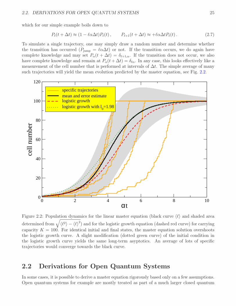
To simulate a single trajectory, one may simply draw a random number and determine whetherthe transition has occurred (Pjump = ℓα∆t) or not. If the transition occurs, we do again havecomplete knowledge and may set Pα(t + ∆t) = δℓ+1,α. If the transition does not occur, we alsohave complete knowledge and remain at Pα(t+∆t) = δℓα. In any case, this looks effectively like ameasurement of the cell number that is performed at intervals of ∆t. The simple average of manysuch trajectories will yield the mean evolution predicted by the master equation, see Fig. 2.2.
0 2 4 6 8 10αt
0
20
40
60
80
100
120
cell
num
ber
specific trajectoriesmean and error estimatelogistic growthlogistic growth with l
0=1.98
Figure 2.2: Population dynamics for the linear master equation (black curve 〈ℓ〉 and shaded area
determined from√
〈ℓ2〉 − 〈ℓ〉2) and for the logistic growth equation (dashed red curve) for carrying
capacity K = 100. For identical initial and final states, the master equation solution overshootsthe logistic growth curve. A slight modification (dotted green curve) of the initial condition inthe logistic growth curve yields the same long-term asyptotics. An average of lots of specifictrajectories would converge towards the black curve.
2.2 Derivations for Open Quantum Systems
In some cases, it is possible to derive a master equation rigorously based only on a few assumptions.Open quantum systems for example are mostly treated as part of a much larger closed quantum

26 CHAPTER 2. OBTAINING A MASTER EQUATION
system (the union of system and bath), where the partial trace is used to eliminate the unwanted(typically many) degrees of freedom of the bath, see Fig. 2.3. Technically speaking, we will consider
Figure 2.3: An open quantum system can be conceived as being part of a larger closed quantumsystem, where the system part (HS) is coupled to the bath (HB) via the interaction HamiltonianHI.
Hamiltonians of the form
H = HS ⊗ 1+ 1⊗HB +HI , (2.8)
where the system and bath Hamiltonians act only on the system and bath Hilbert space, respec-tively. In contrast, the interaction Hamiltonian acts on both Hilbert spaces
HI =∑
α
Aα ⊗ Bα , (2.9)
where the summation boundaries are in the worst case limited by the dimension of the systemHilbert space. As we consider physical observables here, it is required that all Hamiltonians areself-adjoint.
Exercise 13 (Hermiticity of Couplings) (1 points)Show that it is always possible to choose hermitian coupling operators Aα = A†
α and Bα = B†α using
that HI = H†I .
2.2.1 Weak Coupling Regime
When the interaction HI is small, it is justified to apply perturbation theory. The von-Neumannequation in the joint total quantum system
ρ = −i [HS ⊗ 1+ 1⊗HB +HI, ρ] (2.10)
describes the full evolution of the combined density matrix. This equation can be formally solvedby the unitary evolution ρ(t) = e−iHtρ0e
+iHt, which however is impractical to compute as Hinvolves too many degrees of freedom.
Transforming to the interaction picture
ρ(t) = e+i(HS+HB)tρ(t)e−i(HS+HB)t , (2.11)

2.2. DERIVATIONS FOR OPEN QUANTUM SYSTEMS 27
which will be denoted by bold symbols throughout, the von-Neumann equation transforms into
ρ = −i [HI(t),ρ] , (2.12)
where the in general time-dependent interaction Hamiltonian
HI(t) = e+i(HS+HB)tHIe−i(HS+HB)t =
∑
α
e+iHStAαe−iHSt ⊗ e+iHBtBαe
−iHBt
=∑
α
Aα(t)⊗Bα(t) (2.13)
allows to perform perturbation theory.
Born-Markov-Secular Approximations
Without loss of generality we will assume here the case of hermitian coupling operators Aα = A†α
and Bα = B†α. One heuristic way to perform perturbation theory is to formally integrate Eq. (2.13)
and to re-insert the result in the r.h.s. of Eq. (2.13). The time-derivative of the system densitymatrix is obtained by performing the partial trace
ρS = −iTrB [HI(t), ρ0] −t∫
0
TrB [HI(t), [HI(t′),ρ(t′)]] dt′ . (2.14)
This integro-differential equation is still exact but unfortunately not closed as the r.h.s. does notdepend on ρS but the full density matrix at all previous times.
To close the above equation, we employ factorization of the initial density matrix
ρ0 = ρ0S ⊗ ρB (2.15)
together with perturbative considerations: Assuming that HI(t) = Oλ with λ beeing a smalldimensionless perturbation parameter (solely used for bookkeeping purposes here) and that theenvironment is so large such that it is hardly affected by the presence of the system, we mayformally expand the full density matrix
ρ(t) = ρS(t)⊗ ρB +Oλ , (2.16)
where the neglect of all higher orders is known as Born approximation. Eq. (2.14) demonstratesthat the Born approximation is equivalent to a perturbation theory in the interaction Hamiltonian
ρS = −iTrB [HI(t), ρ0] −t∫
0
TrB [HI(t), [HI(t′),ρS(t
′)⊗ ρB]] dt′+Oλ3 . (2.17)
Using the decomposition of the interaction Hamiltonian (2.9), this obviously yields a closed equa-tion for the system density matrix
ρS = −i∑
α
[Aα(t)ρ
0STr Bα(t)ρB − ρ0SAα(t)Tr ρBBα(t)
]−∑
αβ
t∫
0
[
+Aα(t)Aβ(t′)ρS(t
′)Tr Bα(t)Bβ(t′)ρB
−Aα(t)ρS(t′)Aβ(t
′)Tr Bα(t)ρBBβ(t′)
−Aβ(t′)ρS(t
′)Aα(t)Tr Bβ(t′)ρBBα(t)
+ρS(t′)Aβ(t
′)Aα(t)Tr ρBBβ(t′)Bα(t)
]
dt′ . (2.18)

28 CHAPTER 2. OBTAINING A MASTER EQUATION
Without loss of generality, we proceed by assuming that the single coupling operator expectationvalue vanishes
Tr Bα(t)ρB = 0 . (2.19)
This situation can always be constructed by simultaneously modifying system Hamiltonian HS
and coupling operators Aα, see exercise 14.
Exercise 14 (Vanishing single-operator expectation values) (1 points)Show that by modifying system and interaction Hamiltonian
HS → HS +∑
α
gαAα , Bα → Bα − gα1 (2.20)
one can construct a situation where Tr Bα(t)ρB = 0. Determine gα.
Using the cyclic property of the trace, we obtain
ρS = −∑
αβ
t∫
0
dt′[
Cαβ(t, t′) [Aα(t),Aβ(t
′)ρS(t′)]
+Cβα(t′, t) [ρS(t
′)Aβ(t′),Aα(t)]
]
(2.21)
with the bath correlation function
Cαβ(t1, t2) = Tr Bα(t1)Bβ(t2)ρB . (2.22)
The integro-differential equation (2.21) is a non-Markovian master equation, as the r.h.s.depends on the value of the dynamical variable (the density matrix) at all previous times – weightedby the bath correlation functions. It does preserve trace and hermiticity of the system densitymatrix, but not necessarily its positivity. Such integro-differential equations can only be solved invery specific cases. Therefore, we motivate further approximations, for which we need to discussthe analytic properties of the bath correlation functions.
It is quite straightforward to see that when the bath Hamiltonian commutes with the bathdensity matrix [HB, ρB] = 0, the bath correlation functions actually only depend on the differenceof their time arguments Cαβ(t1, t2) = Cαβ(t1 − t2) with
Cαβ(t1 − t2) = Tre+iHB(t1−t2)Bαe
−iHB(t1−t2)Bβ ρB. (2.23)
Since we chose our coupling operators hermitian, we have the additional symmetry that Cαβ(τ) =C∗
βα(−τ). One can now evaluate several system-bath models and when the bath has a densespectrum, the bath correlation functions are typically found to be strongly peaked around zero,see exercise 15.

2.2. DERIVATIONS FOR OPEN QUANTUM SYSTEMS 29
Exercise 15 (Bath Correlation Function) (1 points)Evaluate the Fourier transform γαβ(ω) =
∫Cαβ(τ)e
+iωτdτ of the bath correlation functions for
the coupling operators B1 =∑
k hkbk and B2 =∑
k h∗kb
†k for a bosonic bath HB =
∑
k ωkb†kbk in
the thermal equilibrium state ρ0B = e−βHB
Tre−βHB . You may use the continous representation Γ(ω) =
2π∑
k |hk|2δ(ω − ωk) for the tunneling rates.
This implies that the integro-differential equation (2.21) can also be written as ρS =t∫
0
W(t− t′)ρS(t′)dt′,
where the kernel W(τ) assigns a much smaller weight to density matrices far in the past thanto the density matrix just an instant ago. In the most extreme case, we would approximateCαβ(t1, t2) ≈ Γαβδ(t1 − t2), but we will be cautious here and assume that only the density matrixvaries slower than the decay time of the bath correlation functions. Therefore, we replace in ther.h.s. ρS(t
′) → ρS(t) (first Markov approximation), which yields in Eq. (2.17)
ρS = −t∫
0
TrB [HI(t), [HI(t′),ρS(t)⊗ ρB]] dt′ (2.24)
This equation is often called Born-Redfield equation. It is time-local and preserves trace andhermiticity, but still has time-dependent coefficients (also when transforming back from the inter-action picture). We substitute τ = t− t′
ρS = −t∫
0
TrB [HI(t), [HI(t− τ),ρS(t)⊗ ρB]] dτ (2.25)
= −∑
αβ
t∫
0
Cαβ(τ) [Aα(t),Aβ(t− τ)ρS(t)] + Cβα(−τ) [ρS(t)Aβ(t− τ),Aα(t)] dτ
The problem that the r.h.s. still depends on time is removed by extending the integration boundsto infinity (second Markov approximation) – by the same reasoning that the bath correlationfunctions decay rapidly
ρS = −∞∫
0
TrB [HI(t), [HI(t− τ),ρS(t)⊗ ρB]] dτ . (2.26)
This equation is called the Markovian master equation, which in the original Schrodingerpicture
ρS = −i [HS, ρS(t)]−∑
αβ
∞∫
0
Cαβ(τ)[Aα, e
−iHSτAβe+iHSτρS(t)
]dτ
−∑
αβ
∞∫
0
Cβα(−τ)[ρS(t)e
−iHSτAβe+iHSτ , Aα
]dτ (2.27)
is time-local, preserves trace and hermiticity, and has constant coefficients – best prerequisites fortreatment with established solution methods.
30 CHAPTER 2. OBTAINING A MASTER EQUATION
Exercise 16 (Properties of the Markovian Master Equation) (1 points)Show that the Markovian Master equation (2.27) preserves trace and hermiticity of the densitymatrix.
In addition, it can be obtained easily from the coupling Hamiltonian, since we have not evenused that the coupling operators should be hermitian.
There is just one problem left: In the general case, it is not of Lindblad form. Note thatthere are specific cases where the Markovian master equation is of Lindblad form, but these ratherinclude simple limits. Though this is sometimes considered a rather cosmetic drawback, it maylead to unphysical results such as negative probabilities.
To obtain a Lindblad type master equation, a further approximation is required. The secularapproximation involves an averaging over fast oscillating terms, but in order to identify theoscillating terms, it is necessary to at least formally calculate the interaction picture dynamics ofthe system coupling operators. We begin by writing Eq. (2.27) in the interaction picture againexplicitly – now using the hermiticity of the coupling operators
ρS = −∞∫
0
∑
αβ
Cαβ(τ) [Aα(t),Aβ(t− τ)ρS(t)] + h.c. dτ
= +
∞∫
0
∑
αβ
Cαβ(τ)∑
a,b,c,d
|a〉 〈a|Aβ(t− τ) |b〉 〈b|ρS(t) |d〉 〈d|Aα(t) |c〉 〈c|
− |d〉 〈d|Aα(t) |c〉 〈c| |a〉 〈a|Aβ(t− τ) |b〉 〈b|ρS(t)
dτ + h.c. , (2.28)
where we have introduced the system energy eigenbasis
HS |a〉 = Ea |a〉 . (2.29)
We can use this eigenbasis to make the time-dependence of the coupling operators in the interactionpicture explicit
ρS = +
∞∫
0
∑
αβ
Cαβ(τ)∑
a,b,c,d
e+i(Ea−Eb)(t−τ)e+i(Ed−Ec)t 〈a|Aβ |b〉 〈d|Aα |c〉 |a〉 〈b|ρS(t) |d〉 〈c|
−e+i(Ea−Eb)(t−τ)e+i(Ed−Ec)t 〈a|Aβ |b〉 〈d|Aα |c〉 |d〉 〈c| |a〉 〈b|ρS(t)
dτ + h.c. ,
=∑
αβ
∑
a,b,c,d
∞∫
0
Cαβ(τ)e+i(Eb−Ea)τdτe−i(Eb−Ea−(Ed−Ec))t 〈a|Aβ |b〉 〈c|Aα |d〉∗
+ |a〉 〈b|ρS(t) (|c〉 〈d|)† − (|c〉 〈d|)† |a〉 〈b|ρS(t)
+ h.c. (2.30)
The secular approximation now involves neglecting all terms that are oscillatory in time t

2.2. DERIVATIONS FOR OPEN QUANTUM SYSTEMS 31
(long-time average), i.e., we have
ρS =∑
αβ
∑
a,b,c,d
Γαβ(Eb − Ea)δEb−Ea,Ed−Ec〈a|Aβ |b〉 〈c|Aα |d〉∗ ×
×
+ |a〉 〈b|ρS(t) (|c〉 〈d|)† − (|c〉 〈d|)† |a〉 〈b|ρS(t)
+∑
αβ
∑
a,b,c,d
Γ∗αβ(Eb − Ea)δEb−Ea,Ed−Ec
〈a|Aβ |b〉∗ 〈c|Aα |d〉 ×
×
+ |c〉 〈d|ρS(t) (|a〉 〈b|)† − ρS(t) (|a〉 〈b|)† |c〉 〈d|
, (2.31)
where we have introduced the half-sided Fourier transform of the bath correlation functions
Γαβ(ω) =
∞∫
0
Cαβ(τ)e+iωτdτ . (2.32)
This equation preserves trace, hermiticity, and positivity of the density matrix and hence all desiredproperties, since it is of Lindblad form (which will be shown later). Unfortunately, it is typicallynot so easy to obtain as it requires diagonalization of the system Hamiltonian first. By using thetransformations α ↔ β, a ↔ c, and b ↔ d in the second line and also using that the δ-function issymmetric, we may rewrite the master equation as
ρS =∑
αβ
∑
a,b,c,d
[Γαβ(Eb − Ea) + Γ∗
βα(Eb − Ea)]δEb−Ea,Ed−Ec
×
×〈a|Aβ |b〉 〈c|Aα |d〉∗ |a〉 〈b|ρS(t) (|c〉 〈d|)†
−∑
αβ
∑
a,b,c,d
Γαβ(Eb − Ea)δEb−Ea,Ed−Ec×
×〈a|Aβ |b〉 〈c|Aα |d〉∗ (|c〉 〈d|)† |a〉 〈b|ρS(t)
−∑
αβ
∑
a,b,c,d
Γ∗βα(Eb − Ea)δEb−Ea,Ed−Ec
×
×〈a|Aβ |b〉 〈c|Aα |d〉∗ ρS(t) (|c〉 〈d|)† |a〉 〈b| . (2.33)
We split the matrix-valued function Γαβ(ω) into hermitian and anti-hermitian parts
Γαβ(ω) =1
2γαβ(ω) +
1
2σαβ(ω) ,
Γ∗βα(ω) =
1
2γαβ(ω)−
1
2σαβ(ω) , (2.34)
with hermitian γαβ(ω) = γ∗βα(ω) and anti-hermitian σαβ(ω) = −σ∗
βα(ω). These new functions canbe interpreted as full even and odd Fourier transforms of the bath correlation functions
γαβ(ω) = Γαβ(ω) + Γ∗βα(ω) =
+∞∫
−∞
Cαβ(τ)e+iωτdτ ,
σαβ(ω) = Γαβ(ω)− Γ∗βα(ω) =
+∞∫
−∞
Cαβ(τ)sgn(τ)e+iωτdτ . (2.35)

32 CHAPTER 2. OBTAINING A MASTER EQUATION
Exercise 17 (Odd Fourier Transform) (1 points)Show that the odd Fourier transform σαβ(ω) may be obtained from the even Fourier transformγαβ(ω) by a Cauchy principal value integral
σαβ(ω) =i
πP
+∞∫
−∞
γαβ(Ω)
ω − ΩdΩ .
In the master equation, these replacements lead to
ρS =∑
αβ
∑
a,b,c,d
γαβ(Eb − Ea)δEb−Ea,Ed−Ec〈a|Aβ |b〉 〈c|Aα |d〉∗ ×
×[
|a〉 〈b|ρS(t) (|c〉 〈d|)† −1
2
(|c〉 〈d|)† |a〉 〈b| ,ρS(t)]
−i∑
αβ
∑
a,b,c,d
1
2iσαβ(Eb − Ea)δEb−Ea,Ed−Ec
〈a|Aβ |b〉 〈c|Aα |d〉∗ ×
×[
(|c〉 〈d|)† |a〉 〈b| ,ρS(t)]
=∑
αβ
∑
a,b,c,d
γαβ(Eb − Ea)δEb−Ea,Ed−Ec〈a|Aβ |b〉 〈c|Aα |d〉∗ ×
×[
|a〉 〈b|ρS(t) (|c〉 〈d|)† −1
2
(|c〉 〈d|)† |a〉 〈b| ,ρS(t)]
(2.36)
−i
[∑
αβ
∑
a,b,c
1
2iσαβ(Eb − Ec)δEb,Ea
〈c|Aβ |b〉 〈c|Aα |a〉∗ |a〉 〈b| ,ρS(t)
]
.
To prove that we have a Lindblad form, it is easy to see first that the term in the commutator
HLS =∑
αβ
∑
a,b,c
1
2iσαβ(Eb − Ec)δEb,Ea
〈c|Aβ |b〉 〈c|Aα |a〉∗ |a〉 〈b| (2.37)
is an effective Hamiltonian. This Hamiltonian is often called Lamb-shift Hamiltonian, since itrenormalizes the system Hamiltonian due to the interaction with the reservoir. Note that we have[HS, HLS] = 0.
Exercise 18 (Lamb-shift) (1 points)Show that HLS = H†
LS and [HLS,HS] = 0.
To show the Lindblad-form of the non-unitary evolution, we identify the Lindblad jump op-erator Lα = |a〉 〈b| = L(a,b). For an N -dimensional system Hilbert space with N eigenvectors ofHS we would have N2 such jump operators, but in a rotated basis, we may leave out the identitymatrix 1 =
∑
a |a〉 〈a| (which has trivial action). It remains to be shown that the matrix
γ(ab),(cd) =∑
αβ
γαβ(Eb − Ea)δEb−Ea,Ed−Ec〈a|Aβ |b〉 〈c|Aα |d〉∗ (2.38)

2.2. DERIVATIONS FOR OPEN QUANTUM SYSTEMS 33
is non-negative, i.e.,∑
a,b,c,d x∗abγ(ab),(cd)xcd ≥ 0 for all xab. We first note that for hermitian coupling
operators the Fourier transform matrix at fixed ω is positive (recall that Bα = B†α and [ρB,HB] = 0)
Γ =∑
αβ
x∗αγαβ(ω)xβ
=
+∞∫
−∞
dτe+iωτTr
eiHSτ
[∑
α
x∗αBα
]
e−iHSτ
[∑
β
xβBβ
]
ρB
=
+∞∫
−∞
dτe+iωτ∑
nm
e+i(En−Em)τ 〈n|B† |m〉 〈m|BρB |n〉
=∑
nm
2πδ(ω + En − Em)|〈m|B |n〉|2ρn
≥ 0 . (2.39)
Now, we replace the Kronecker symbol in the dampening coefficients by two via the introductionof an auxiliary summation
Γ =∑
abcd
x∗abγ(ab),(cd)xcd
=∑
ω
∑
αβ
∑
abcd
γαβ(ω)δEb−Ea,ωδEd−Ec,ωx∗ab 〈a|Aβ |b〉 xcd 〈c|Aα |d〉∗
=∑
ω
∑
αβ
[∑
cd
xcd 〈c|Aα |d〉∗ δEd−Ec,ω
]
γαβ(ω)
[∑
ab
x∗ab 〈a|Aβ |b〉 δEb−Ea,ω
]
=∑
ω
∑
αβ
y∗α(ω)γαβ(ω)yβ(ω) ≥ 0 . (2.40)
Transforming Eq. (2.36) back to the Schrodinger picture (note that the δ-functions prohibitthe occurrence of oscillatory factors), we finally obtain the Born-Markov-secular master equation.
Box 7 (BMS master equation) In the weak coupling limit, an interaction Hamiltonian of theform HI =
∑
α Aα⊗Bα with hermitian coupling operators (Aα = A†α and Bα = B†
α) and [HB, ρB] =0 and Tr BαρB = 0 leads in the system energy eigenbasis HS |a〉 = Ea |a〉 to the Lindblad-formmaster equation
ρS = −i
[
HS +∑
ab
σab |a〉 〈b| , ρS(t)]
+∑
a,b,c,d
γab,cd
[
|a〉 〈b|ρS(t) (|c〉 〈d|)† −1
2
(|c〉 〈d|)† |a〉 〈b| ,ρS(t)]
,
γab,cd =∑
αβ
γαβ(Eb − Ea)δEb−Ea,Ed−Ec〈a|Aβ |b〉 〈c|Aα |d〉∗ , (2.41)
where the Lamb-shift Hamiltonian HLS =∑
ab σab |a〉 〈b| matrix elements read
σab =∑
αβ
∑
c
1
2iσαβ(Eb − Ec)δEb,Ea
〈c|Aβ |b〉 〈c|Aα |a〉∗ (2.42)

34 CHAPTER 2. OBTAINING A MASTER EQUATION
and the constants are given by even and odd Fourier transforms
γαβ(ω) =
+∞∫
−∞
Cαβ(τ)e+iωτdτ ,
σαβ(ω) =
+∞∫
−∞
Cαβ(τ)sgn(τ)e+iωτdτ =
i
πP
+∞∫
−∞
γαβ(ω′)
ω − ω′ dω′ (2.43)
of the bath correlation functions
Cαβ(τ) = Tre+iHBτBαe
−iHBτBβ ρB. (2.44)
The above definition may serve as a recipe to derive a Lindblad type master equation in theweak-coupling limit. It is expected to yield good results in the weak coupling and Markovian limit(continuous and nearly flat bath spectral density) and when [ρB,HB] = 0. It requires to rewritethe coupling operators in hermitian form, the calculation of the bath correlation function Fouriertransforms, and the diagonalization of the system Hamiltonian.
In the case that the spectrum of the system Hamiltonian is non-degenerate, we have a furthersimplification, since the δ-functions simplify further, e.g. δEb,Ea
→ δab. By taking matrix elementsof Eq. (2.41) in the energy eigenbasis ρaa = 〈a| ρS |a〉, we obtain an effective rate equation for thepopulations only
ρaa = +∑
b
γab,abρbb −[∑
b
γba,ba
]
ρaa , (2.45)
i.e., the coherences decouple from the evolution of the populations. The transition rates from stateb to state a reduce in this case to
γab,ab =∑
αβ
γαβ(Eb − Ea) 〈a|Aβ |b〉 〈a|Aα |b〉∗ , (2.46)
which – after inserting all definitions condenses basically to Fermis Golden Rule. A description ofopen quantum systems is in this limit possible with the same complexity as for closed quantumsystems, since only N dynamical variables have to be evolved. Also, this may serve to demonstratethe correspondence between quantum and classical mechanics: If only diagonals of the densitymatrix remain in the (orthogonal) energy system eigenbasis, this implies that the quantum masterequation boils down to a classical rate equation. Even more, if coupled to a single thermal bath,the quantum system simply relaxes to the Gibbs equilibrium, i.e., we obtain simply equilibrationof the system temperature with the temperature of the bath.
Coarse-Graining
Although the BMS approximation respects of course the exact initial condition, we have in thederivation made several long-term approximations. For example, the Markov approximation im-plied that we consider timescales much larger than the decay time of the bath correlation functions.Similarly, the secular approximation implied timescales larger than the inverse minimal splitting

2.2. DERIVATIONS FOR OPEN QUANTUM SYSTEMS 35
of the system energy eigenvalues. Therefore, we can only expect the solution originating from theBMS master equation to be an asymptotically valid long-term approximation.
Coarse-graining in contrast provides a possibility to obtain valid short-time approximationsof the density matrix with a generator that is of Lindblad form, see Fig. 2.4. We start with the
Figure 2.4: Sketch of the coarse-graining perturbation theory. Calculating the exact time evolution
operator U (t) = τ exp
−it∫
0
HI(t′)dt′
in a closed form is usually prohibitive, which renders the
calculation of the exact solution an impossible task (black curve). It is however possible to expand
the evolution operator U2(t) = 1−it∫
0
HI(t′)dt′−
t∫
0
dt1dt2HI(t1)HI(t2)Θ(t1−t2) to second order in
HI and to obtain the corresponding reduced approximate density matrix. Calculating the matrixexponential of a constant Lindblad-type generator LCG
τ is also usually prohibitive, but the firstorder approximation may be matched with U2(t) at time t = τ to obtain a defining equation forLCG
τ .
von-Neumann equation in the interaction picture (2.12). For factorizing initial density matrices,it is formally solved by U (t)ρ0S ⊗ ρBU
†(t), where the time evolution operator
U (t) = τ exp
−i
t∫
0
HI(t′)dt′
(2.47)
obeys the evolution equation
U = −iHI(t)U(t) , (2.48)
which defines the time-ordering operator τ . Formally integrating this equation with the evident

36 CHAPTER 2. OBTAINING A MASTER EQUATION
initial condition U (0) = 1 yields
U (t) = 1− i
t∫
0
HI(t′)U(t′)dt′
= 1− i
t∫
0
HI(t′)dt′ −
t∫
0
dt′HI(t′)
t′∫
0
dt′′HI(t′′)U (t′′)
≈ 1− i
t∫
0
HI(t′)dt′ −
t∫
0
dt1dt2HI(t1)HI(t2)Θ(t1 − t2) , (2.49)
where the occurrence of the Heaviside function is a consequence of time-ordering. For the hermitianconjugate operator we obtain
U †(t) ≈ 1+ i
t∫
0
HI(t′)dt′ −
t∫
0
dt1dt2HI(t1)HI(t2)Θ(t2 − t1) . (2.50)
To keep the discussion at a moderate level, we assume Tr BαρB = 0 from the beginning. Theexact solution is approximated by
ρ(2)S (t) ≈ TrB
1− i
t∫
0
HI(t1)dt1 −t∫
0
dt1dt2HI(t1)HI(t2)Θ(t1 − t2)
ρ0S ⊗ ρB ×
×
1+ i
t∫
0
HI(t1)dt1 −t∫
0
dt1dt2HI(t1)HI(t2)Θ(t2 − t1)
= ρ0S − iTrB
t∫
0
HI(t1)dt1, ρ0S ⊗ ρB
+TrB
t∫
0
dt1
t∫
0
dt2HI(t1)ρ0S ⊗ ρBHI(t2)
−t∫
0
dt1dt2[Θ(t1 − t2)HI(t1)HI(t2)ρ
0S ⊗ ρB +Θ(t2 − t1)ρ
0S ⊗ ρBHI(t1)HI(t2)
].
(2.51)
Again, we introduce the bath correlation functions with two time arguments as in Eq. (2.22)
Cαβ(t1, t2) = Tr Bα(t1)Bβ(t2)ρB , (2.52)
such that we have
ρ(2)S (t) = ρ0S +
∑
αβ
t∫
0
dt1
t∫
0
dt2Cαβ(t1, t2)[
Aβ(t2)ρ0SAα(t1)
−Θ(t1 − t2)Aα(t1)Aβ(t2)ρ0S −Θ(t2 − t1)ρ
0SAα(t1)Aβ(t2)
]
. (2.53)

2.2. DERIVATIONS FOR OPEN QUANTUM SYSTEMS 37
At time t, this should for weak-coupling match the evolution by a Markovian generator
ρSCG(τ) = eL
CGτ ·τρ0S ≈
[1+ LCG
τ · τ]ρ0S , (2.54)
such that we can infer the action of the generator on an arbitrary density matrix
LCGτ ρS =
1
τ
∑
αβ
τ∫
0
dt1
τ∫
0
dt2Cαβ(t1, t2)[
Aβ(t2)ρSAα(t1)
−Θ(t1 − t2)Aα(t1)Aβ(t2)ρS −Θ(t2 − t1)ρSAα(t1)Aβ(t2)]
= −i
1
2iτ
τ∫
0
dt1
τ∫
0
dt2∑
αβ
Cαβ(t1, t2)sgn(t1 − t2)Aα(t1)Aβ(t2),ρS
+1
τ
τ∫
0
dt1
τ∫
0
dt2∑
αβ
Cαβ(t1, t2)
[
Aβ(t2)ρSAα(t1)−1
2Aα(t1)Aβ(t2),ρS
]
,(2.55)
where we have inserted Θ(x) = 12[1 + sgn(x)].
Box 8 (CG Master Equation) In the weak coupling limit, an interaction Hamiltonian of theform HI =
∑
α Aα ⊗ Bα leads to the Lindblad-form master equation in the interaction picture
ρS = −i
1
2iτ
τ∫
0
dt1
τ∫
0
dt2∑
αβ
Cαβ(t1, t2)sgn(t1 − t2)Aα(t1)Aβ(t2),ρS
+1
τ
τ∫
0
dt1
τ∫
0
dt2∑
αβ
Cαβ(t1, t2)
[
Aβ(t2)ρSAα(t1)−1
2Aα(t1)Aβ(t2),ρS
]
,
where the bath correlation functions are given by
Cαβ(tt, t2) = Tre+iHBt1Bαe
−iHBt1e+iHBt2Bβe−iHBt2 ρB
. (2.56)
We have not used hermiticity of the coupling operators nor that the bath correlation functionsdo typically only depend on a single argument. However, if the coupling operators were chosenhermitian, it is easy to show the Lindblad form. Obtaining the master equation requires the calcu-lation of bath correlation functions and the evolution of the coupling operators in the interactionpicture.
Exercise 19 (Lindblad form) (1 point)By assuming hermitian coupling operators Aα = A†
α, show that the CG master equation is ofLindblad form for all coarse-graining times τ .

38 CHAPTER 2. OBTAINING A MASTER EQUATION
Let us make once more the time-dependence of the coupling operators explicit, which is mostconveniently done in the system energy eigenbasis. Now, we also assume that the bath correlationfunctions only depend on the difference of their time arguments Cαβ(t1, t2) = Cαβ(t1 − t2), suchthat we may use the Fourier transform definitions in Eq. (2.35) to obtain
ρS = −i
1
2iτ
∑
abc
τ∫
0
dt1
τ∫
0
dt2∑
αβ
Cαβ(t1 − t2)sgn(t1 − t2) |a〉 〈a|Aα(t1) |c〉 〈c|Aβ(t2) |b〉 〈b| ,ρS
+1
τ
τ∫
0
dt1
τ∫
0
dt2∑
αβ
∑
abcd
Cαβ(t1 − t2)[
|a〉 〈a|Aβ(t2) |b〉 〈b|ρS |d〉 〈d|Aα(t1) |c〉 〈c|
−1
2|d〉 〈d|Aα(t1) |c〉 〈c| · |a〉 〈a|Aβ(t2) |b〉 〈b| ,ρS
]
= −i1
4iπτ
∫
dω∑
abc
τ∫
0
dt1
τ∫
0
dt2∑
αβ
σαβ(ω)e−iω(t1−t2)e+i(Ea−Ec)t1e+i(Ec−Eb)t2 ×
×〈c|Aβ |b〉 〈c|A†α |a〉∗ [|a〉 〈b| ,ρS]
+1
2πτ
∫
dω
τ∫
0
dt1
τ∫
0
dt2∑
αβ
∑
abcd
γαβ(ω)e−iω(t1−t2)e+i(Ea−Eb)t2e+i(Ed−Ec)t1 〈a|Aβ |b〉 〈c|A†
α |d〉∗ ×
×[
|a〉 〈b|ρS (|c〉 〈d|)† −1
2
(|c〉 〈d|)† |a〉 〈b| ,ρS
]
. (2.57)
We perform the temporal integrations by invoking
τ∫
0
eiαktkdtk = τeiαkτ/2sinc[αkτ
2
]
(2.58)
with sinc(x) = sin(x)/x to obtain
ρS = −iτ
4iπ
∫
dω∑
abc
∑
αβ
σαβ(ω)eiτ(Ea−Eb)/2sinc
[τ
2(Ea − Ec − ω)
]
sinc[τ
2(Ec − Eb + ω)
]
×
×〈c|Aβ |b〉 〈c|A†α |a〉∗ [|a〉 〈b| ,ρS]
+τ
2π
∫
dω∑
αβ
∑
abcd
γαβ(ω)eiτ(Ea−Eb+Ed−Ec)/2sinc
[τ
2(Ed − Ec − ω)
]
sinc[τ
2(ω + Ea − Eb)
]
×
×〈a|Aβ |b〉 〈c|A†α |d〉∗
[
|a〉 〈b|ρS (|c〉 〈d|)† −1
2
(|c〉 〈d|)† |a〉 〈b| ,ρS
]
. (2.59)
Therefore, we have the same structure as before, but now with coarse-graining time dependentdampening coefficients
ρS = −i
[∑
ab
στab |a〉 〈b| ,ρS
]
+∑
abcd
γτab,cd
[
|a〉 〈b|ρS (|c〉 〈d|)† −1
2
(|c〉 〈d|)† |a〉 〈b| ,ρS
]
(2.60)

2.2. DERIVATIONS FOR OPEN QUANTUM SYSTEMS 39
with the coefficients
στab =
1
2i
∫
dω∑
c
eiτ(Ea−Eb)/2τ
2πsinc
[τ
2(Ea − Ec − ω)
]
sinc[τ
2(Eb − Ec − ω)
]
×
×[∑
αβ
σαβ(ω) 〈c|Aβ |b〉 〈c|A†α |a〉∗
]
,
γτab,cd =
∫
dωeiτ(Ea−Eb+Ed−Ec)/2τ
2πsinc
[τ
2(Ed − Ec − ω)
]
sinc[τ
2(Eb − Ea − ω)
]
×
×[∑
αβ
γαβ(ω) 〈a|Aβ |b〉 〈c|A†α |d〉∗
]
. (2.61)
Finally, we note that in the limit of large coarse-graining times τ → ∞, these dampening coefficientsconverge to the ones in definition 7, i.e.,
limτ→∞
στab = σab ,
limτ→∞
γτab,cd = γab,cd . (2.62)
Exercise 20 (CG-BMS correspondence) (1 points)Show for hermitian coupling operators that when τ → ∞, CG and BMS approximation are equiv-alent. You may use the identity
limτ→∞
τsinc[τ
2(Ωa − ω)
]
sinc[τ
2(Ωb − ω)
]
= 2πδΩa,Ωbδ(Ωa − ω) .
Thermalization
The BMS limit has beyond its relatively compact Lindblad form further appealing properties inthe case of a bath that is in thermal equilibrium
ρB =e−βHB
Tr e−βHB (2.63)
with inverse temperature β. These root in further analytic properties of the bath correlationfunctions such as the Kubo-Martin-Schwinger (KMS) condition
Cαβ(τ) = Cβα(−τ − iβ) . (2.64)
Exercise 21 (KMS condition) (1 points)
Show the validity of the KMS condition for a thermal bath with ρB = e−βHB
Tre−βHB .

40 CHAPTER 2. OBTAINING A MASTER EQUATION
For the Fourier transform, this shift property implies
γαβ(−ω) =
+∞∫
−∞
Cαβ(τ)e−iωτdτ =
+∞∫
−∞
Cβα(−τ − iβ)e−iωτdτ
=
−∞−iβ∫
+∞−iβ
Cβα(τ′)e+iω(τ ′+iβ)(−)dτ ′ =
+∞−iβ∫
−∞−iβ
Cβα(τ′)e+iωτ ′dτ ′e−βω
=
+∞∫
−∞
Cβα(τ′)e+iωτ ′dτ ′e−βω = γβα(+ω)e−βω , (2.65)
where in the last line we have used that the bath correlation functions are analytic in τ in the com-plex plane and vanish at infinity, such that we may safely deform the integration contour. Finally,the KMS condition can thereby be used to prove that for a reservoir with inverse temperature β,the density matrix
ρS =e−βHS
Tr e−βHS (2.66)
is one stationary state of the BMS master equation (and the τ → ∞ limit of the CG appraoch).
Exercise 22 (Thermalization) (1 points)
Show that ρS = e−βHS
Tre−βHS is a stationary state of the BMS master equation, when γαβ(−ω) =
γβα(+ω)e−βω.
When the reservoir is in the grand-canonical equilibrium state
ρB =e−β(HB−µNB)
Tr e−β(HB−µNB) , (2.67)
where N = NS +NBis a conserved quantity [HS +HB +HI, NS +NB] = 0, the KMS condition isnot fulfilled anymore. However, even in this case one can show that a stationary state of the BMSmaster equation is given by
ρS =e−β(HS−µNS)
Tr e−β(HS−µNS) , (2.68)
i.e., both temperature β and chemical potential µ equilibrate.
2.2.2 Strong-coupling regime
So far we have considered the situation where the interaction Hamiltonian was the weakest part.One may easily generalize to a situation where the system Hamiltonian is weakest, i.e., formallywe are interested in the limit ǫ → 0 where H = HS + ǫ−1HI + ǫ−2HB. The derivation based onthe conventional Born, and Markov approximations is performed in complete analogy, except that

2.2. DERIVATIONS FOR OPEN QUANTUM SYSTEMS 41
the secular approximation is not necessary, since in the considered limit, all system energies areeffectively zero.
We start in the same interaction picture and perform Born- and Markov approximations, seeEq. (2.27). Now however, the system density matrix changes much faster even than the systemcoupling operators, such that we may effectively replace e±HSτ → 1
ρS = −i [HS, ρS]−∑
αβ
∞∫
0
Cαβ(τ) [Aα, AβρS(t)] dτ −∑
αβ
∞∫
0
Cβα(τ) [Aα, ρS(t)Aβ] dτ . (2.69)
It is straightforward (for hermitian coupling operators) to show that this expression is of Lindbladform.
Box 9 (Singular Coupling Limit) In the singular coupling limit, an interaction Hamiltonianof the form HI =
∑
α Aα ⊗ Bα with hermitian coupling operators (Aα = A†α and Bα = B†
α) and[HB, ρB] = 0 and Tr BαρB = 0 leads to the Lindblad-form master equation
ρS = −i
[
HS +∑
αβ
1
2iσαβ(0)AαAβ, ρS(t)
]
+∑
αβ
γαβ(0)
[
AαρS(t)Aβ −1
2AβAα,ρS(t)
]
,(2.70)
where the constants are given by
γαβ(0) =
+∞∫
−∞
Tre+iHBτBαe
−iHBτBβρBdτ ,
σαβ(0) =
+∞∫
−∞
Tre+iHBτBαe
−iHBτBβρBsgn(τ)dτ . (2.71)
Formally, the singular coupling limit may also be obtained from the BMS limit by setting allsystem energies to zero.

42 CHAPTER 2. OBTAINING A MASTER EQUATION
Chapter 3
Solving Master Equations
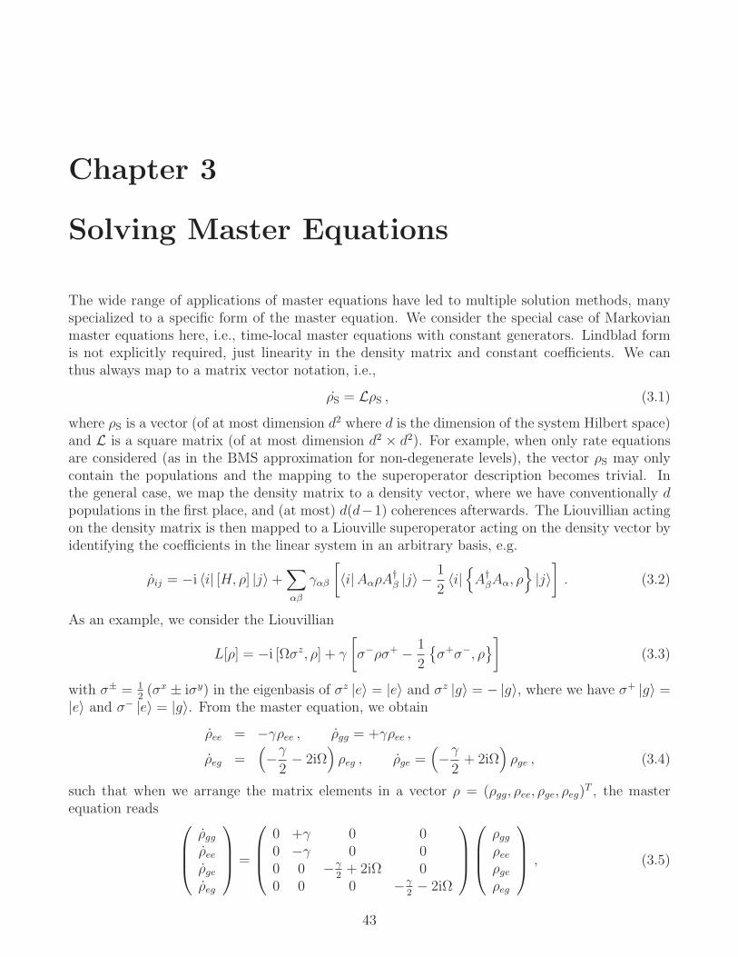
The wide range of applications of master equations have led to multiple solution methods, manyspecialized to a specific form of the master equation. We consider the special case of Markovianmaster equations here, i.e., time-local master equations with constant generators. Lindblad formis not explicitly required, just linearity in the density matrix and constant coefficients. We canthus always map to a matrix vector notation, i.e.,
ρS = LρS , (3.1)
where ρS is a vector (of at most dimension d2 where d is the dimension of the system Hilbert space)and L is a square matrix (of at most dimension d2 × d2). For example, when only rate equationsare considered (as in the BMS approximation for non-degenerate levels), the vector ρS may onlycontain the populations and the mapping to the superoperator description becomes trivial. Inthe general case, we map the density matrix to a density vector, where we have conventionally dpopulations in the first place, and (at most) d(d−1) coherences afterwards. The Liouvillian actingon the density matrix is then mapped to a Liouville superoperator acting on the density vector byidentifying the coefficients in the linear system in an arbitrary basis, e.g.
ρij = −i 〈i| [H, ρ] |j〉+∑
αβ
γαβ
[
〈i|AαρA†β |j〉 −
1
2〈i|
A†βAα, ρ
|j〉]
. (3.2)
As an example, we consider the Liouvillian
L[ρ] = −i [Ωσz, ρ] + γ
[
σ−ρσ+ − 1
2
σ+σ−, ρ
]
(3.3)
with σ± = 12(σx ± iσy) in the eigenbasis of σz |e〉 = |e〉 and σz |g〉 = − |g〉, where we have σ+ |g〉 =
|e〉 and σ− |e〉 = |g〉. From the master equation, we obtain
ρee = −γρee , ρgg = +γρee ,
ρeg =(
−γ
2− 2iΩ
)
ρeg , ρge =(
−γ
2+ 2iΩ
)
ρge , (3.4)
such that when we arrange the matrix elements in a vector ρ = (ρgg, ρee, ρge, ρeg)T , the master
equation reads
ρggρeeρgeρeg
=
0 +γ 0 00 −γ 0 00 0 −γ
2+ 2iΩ 0
0 0 0 −γ2− 2iΩ
ρggρeeρgeρeg
, (3.5)
43

44 CHAPTER 3. SOLVING MASTER EQUATIONS
such that populations and coherences evolve apparently independently. Note however, that theLindblad form nevertheless ensures for a positive density matrix – valid initial conditions provided.
Exercise 23 (Preservation of Positivity) (1 points)Show that the superoperator in Eq. (3.5) preserves positivity of the density matrix provided that
initial positivity (−1/4 ≤∣∣ρ0ge∣∣2 − ρ0ggρ
0ee ≤ 0) is given.
The expectation value of an operator A is then mapped to a product with the trace vector.
Exercise 24 (Expectation values from superoperators) (1 points)Show that for a Liouvillian superoperator connecting N populations (diagonal entries) with Mcoherences (off-diagonal entries) acting on the density matrix ρ(t) = (P1, . . . , PN , C1, . . . , CM)T ,the trace in the expectation value of an operator can be mapped to the matrix element
〈A(t)〉 = (1, . . . , 1︸ ︷︷ ︸
N×
, 0, . . . , 0︸ ︷︷ ︸
M×
) · A · ρ(t) ,
where the matrix A is the superoperator corresponding to A.
3.1 Analytic Techniques
3.1.1 Full analytic solution with the Matrix Exponential
Trivially, as we have a linear system with constant coefficients, we may obtain the solution of themaster equation via
ρ(t) = eLtρ0 , (3.6)
such that one would have to calculate the matrix exponential. This is usually quite difficult andconstrained to very small dimensions of L, escpecially since the Liouville superoperator L is nothermitian such that it is no spectral decomposition.
Exercise 25 (Single Resonant Level) (1 points)Calculate the matrix exponential of the Liouvillian superoperator for a single resonant level tunnel-coupled to a single junction
L =
(−Γf +Γ(1− f)+Γf −Γ(1− f)
)
when the dot level is much lower than the Fermi edge (f → 1) and when it is much larger than theFermi edge f → 0.
3.1. ANALYTIC TECHNIQUES 45
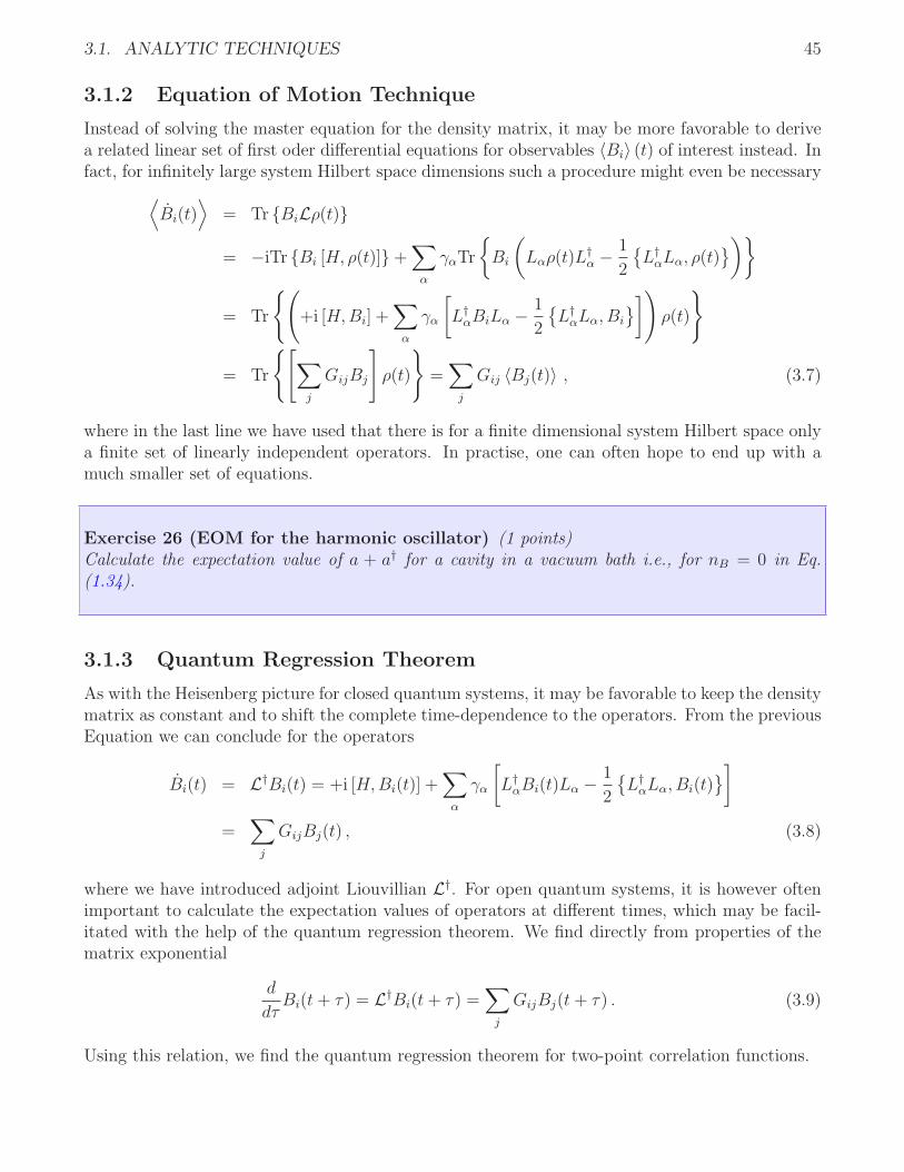
3.1.2 Equation of Motion Technique
Instead of solving the master equation for the density matrix, it may be more favorable to derivea related linear set of first oder differential equations for observables 〈Bi〉 (t) of interest instead. Infact, for infinitely large system Hilbert space dimensions such a procedure might even be necessary
⟨
Bi(t)⟩
= Tr BiLρ(t)
= −iTr Bi [H, ρ(t)]+∑
α
γαTr
Bi
(
Lαρ(t)L†α − 1
2
L†αLα, ρ(t)
)
= Tr
(
+i [H,Bi] +∑
α
γα
[
L†αBiLα − 1
2
L†αLα, Bi
])
ρ(t)
= Tr
[∑
j
GijBj
]
ρ(t)
=∑
j
Gij 〈Bj(t)〉 , (3.7)
where in the last line we have used that there is for a finite dimensional system Hilbert space onlya finite set of linearly independent operators. In practise, one can often hope to end up with amuch smaller set of equations.
Exercise 26 (EOM for the harmonic oscillator) (1 points)Calculate the expectation value of a + a† for a cavity in a vacuum bath i.e., for nB = 0 in Eq.(1.34).
3.1.3 Quantum Regression Theorem
As with the Heisenberg picture for closed quantum systems, it may be favorable to keep the densitymatrix as constant and to shift the complete time-dependence to the operators. From the previousEquation we can conclude for the operators
Bi(t) = L†Bi(t) = +i [H,Bi(t)] +∑
α
γα
[
L†αBi(t)Lα − 1
2
L†αLα, Bi(t)
]
=∑
j
GijBj(t) , (3.8)
where we have introduced adjoint Liouvillian L†. For open quantum systems, it is however oftenimportant to calculate the expectation values of operators at different times, which may be facil-itated with the help of the quantum regression theorem. We find directly from properties of thematrix exponential
d
dτBi(t+ τ) = L†Bi(t+ τ) =
∑
j
GijBj(t+ τ) . (3.9)
Using this relation, we find the quantum regression theorem for two-point correlation functions.

46 CHAPTER 3. SOLVING MASTER EQUATIONS
Box 10 (Quantum Regression) Let single observables follow the closed equation⟨
Bi
⟩
=∑
j Gij 〈Bj〉. Then, the two-point correlation functions obey the equations
d
dτ〈Bi(t+ τ)Bℓ(t)〉 =
∑
j
Gij 〈Bj(t+ τ)Bℓ(t)〉 (3.10)
with exactly the same coefficient matrix Gij.
The advantage of the Quantum regression theorem is that it enables the calculation of ex-pressions for two-point correlation functions just from the evolution of single-operator correlationfunctions.
Let us consider the example of an SET at infinite bias (fL → 1 and fR → 0). The single-operator expectation values obey
d
dt
( ⟨dd†(t)
⟩
⟨d†d(t)
⟩
)
=
(−ΓL +ΓR
+ΓL −ΓR
)( ⟨dd†(t)
⟩
⟨d†d(t)
⟩
)
, (3.11)
such that the quantum regression theorem tells us
d
dτ
( ⟨dd†(t+ τ)d†d(t)
⟩
⟨d†d(t+ τ)d†d(t)
⟩
)
=
(−ΓL +ΓR
+ΓL −ΓR
)( ⟨dd†(t+ τ)d†d(t)
⟩
⟨d†d(t+ τ)d†d(t)
⟩
)
. (3.12)
3.2 Numerical Techniques
3.2.1 Numerical Integration
Numerical integration is generally performed by discretizing time into sufficiently small steps. Notethat there are different discretization schemes, e.g. explicit ones
ρ(t+∆t)− ρ(t)
∆t= Lρ(t) , (3.13)
where the right hand side depends on time t and implicit ones as e.g.
ρ(t+∆t)− ρ(t)
∆t= L1
2[ρ(t) + ρ(t+∆t)] , (3.14)
which first have to be solved (typically requiring matrix inversion) for ρ(t+∆t) to propagate thesolution from time t to time t+∆t. As a rule of thumb, explicit schemes are easy to implement butmay be numerically unstable (i.e., an adaptive stepsize may be required to bound the numericalerror). In contrast, implicit schemes are usually more stable but require a lot of effort to propagatethe solution. Here, we will just discuss a fourth-order Runge-Kutta solver.
In order to propagate a density matrix ρn at time t, to the density matrix ρn+1 at time t+∆t,

3.2. NUMERICAL TECHNIQUES 47
the fourth-order Runge-Kutta scheme proceeds requires the evaluation of some intermediate values
σn,1 = ∆tLρn ,
σn,2 = ∆tL(
ρn +1
2σn,1
)
,
σn,3 = ∆tL(
ρn +1
2σn,2
)
,
σn,4 = ∆tL (ρn + σn,3) ,
ρn+1 = ρn +1
6σn,1 +
1
3σn,2 +
1
3σn,3 +
1
6σn,4 +O∆t5 . (3.15)
This explicit scheme requires four matrix-vector multiplications per timestep. It should always beused with an adaptive stepsize, which can be controlled by comparing (e.g. by computing the normof the difference) the result from two successive propagations with stepsize ∆t with the result of asingle propagation with stepsize 2∆t. If the difference between solutions is too large, the stepsizemust be reduced (and the intermediate result should be discarded). If it is not too large, theresult can always be accepted. In case the error estimate is too small, the stepsize can later-on becautiously increased.
Exercise 27 (Order of the RK scheme) (1 points)Acting with the Liouville superoperator performs the time-derivative of the density matrix. Showthat the presented scheme (3.15) is of fourth order in ∆t, i.e., that
ρn+1 =
[
1+ L∆t+ L2∆t2
2!+ L3∆t3
3!+ L4∆t4
4!
]
ρn .
3.2.2 Simulation as a Piecewise Deterministic Process (PDP)
Suppose we would like to solve the Lindblad form master equation (in diagonal representation)
ρ = −i [H, ρ] +∑
α
γα
[
LαρL†α − 1
2
ρ, L†
α, Lα
]
(3.16)
numerically but do not have the possibility to store the N2 matrix elements of the density matrix.Instead, the master equation can be unravelled to a piecewise deterministic process for a pure
quantum state. The advantage here lies in the fact that a pure state requires only N complexobservables to be evolved.
Consider the nonlinear but deterministic equation
˙|Ψ〉 = −i
[
H − i
2
∑
α
γαL†αLα
]
|Ψ〉+ 1
2
[∑
α
γα 〈Ψ|L†αLα |Ψ〉
]
|Ψ〉 . (3.17)
Although this is nonlinear in |Ψ(t)〉, one can show that the solution is given by
|Ψ〉 = e−iMt |Ψ0〉〈Ψ0| e+iM†te−iMt |Ψ0〉1/2
, (3.18)

48 CHAPTER 3. SOLVING MASTER EQUATIONS
where we have used the operator M = H − i2
∑
α γαL†αLα, which is also often interpreted as a
non-hermitian Hamiltonian.
Exercise 28 (Norm for continuous evolution) (1 points)Calculate the norm of the state vector 〈Ψ(t)|Ψ(t)〉 from Eq. (3.18).
We show the validity of the solution by differentiation
∣∣∣Ψ⟩
= −iM |Ψ〉 − 1
2
e−iMt |Ψ0〉〈Ψ0| e+iM†te−iMt |Ψ0〉3/2
i[
〈Ψ0| e+iM†tM †e−iMt |Ψ0〉 − 〈Ψ0| e+iM†tMe−iMt |Ψ0〉]
= −iM |Ψ〉 − 1
2
e−iMt |Ψ0〉〈Ψ0| e+iM†te−iMt |Ψ0〉3/2
i 〈Ψ0| e+iM†t[M † −M
]e−iMt |Ψ0〉
= −iM |Ψ〉+ 1
2
e−iMt |Ψ0〉〈Ψ0| e+iM†te−iMt |Ψ0〉3/2
∑
α
γα 〈Ψ0| e+iM†tL†αLαe
−iMt |Ψ0〉
= −iM |Ψ〉+ 1
2|Ψ〉
∑
α
γα 〈Ψ|L†αLα |Ψ〉 . (3.19)
However, the name PDP already suggests that the process is only piecewise deterministic.Hence, it will be interruppted by stochastic events. The total probability that a jump of the wavefunction will occur in the infinitesimal interval [t, t+∆t] is given by given by
Pjump = ∆t∑
α
γα 〈Ψ|L†αLα |Ψ〉 . (3.20)
That is, if a jump has occurred, one still has to decide which jump. Choosing a particular jump
|Ψ〉 → Lα |Ψ〉√
〈Ψ|L†αLα |Ψ〉
(3.21)
is performed randomly with conditional probability
Pα =γα 〈Ψ|L†
αLα |Ψ〉∑
α γα 〈Ψ|L†αLα |Ψ〉
, (3.22)
where the normalization is obvious. This recipe for deterministic (continuous) and jump evolutionsmay also be written as a single stochastic differential equation, which is often called stochasticSchrodinger equation.
Box 11 (Stochastic Schrodinger Equation) A Lindblad type master equation of the form
ρ = −i [H, ρ] +∑
α
γα
[
LαρL†α − 1
2
ρ, L†
α, Lα
]
(3.23)

3.2. NUMERICAL TECHNIQUES 49
can be effectively modeled by the stochastic differential equation
|dΨ〉 =
[
−iH − 1
2
∑
α
γαL†αLα +
1
2
∑
α
γα 〈Ψ|L†αLα |Ψ〉
]
|Ψ〉 dt
+∑
α
Lα |Ψ〉
√
〈Ψ|L†αLα |Ψ〉
− |Ψ〉
dNα , (3.24)
where the Poisson increments dNα satisfy
dNαdNβ = δαβdNα , E (dNα) = γα 〈Ψ|L†αLα |Ψ〉 dt (3.25)
and E (x) denotes the classical expectation value (ensemble average).
The last two equations simply mean that at most a single jump can occur at once (practi-cally we have dNα ∈ 0, 1) and that the probability for a jump at time t is given by Pα =γα 〈Ψ|L†
αLα |Ψ〉 dt. Numerically, it constitutes a simple recipe, see Fig. 3.1.
jump
no jump
which jump
Figure 3.1: Recipe for propagating the stochastic Schrodinger equation in Box 11. At each timestepone can calculate the total probability of a jump occuring during the next timestep. Drawing arandom number yields whether a jump should occur or not. Given that a jump occurs, we determinewhich jump by drawing another random number: Setting the particular dNα = 1 and dt = 0 wesolve for |Ψ(t+∆t)〉 = |Ψ(t)〉+ |dΨ(t)〉 and proceed with the next timestep. Given that no jumpoccurs, we simply set dNα = 0 for all α, solve for |Ψ(t+∆t)〉 = |Ψ(t)〉+ |dΨ(t)〉 and proceed withthe next timestep.
It remains to be shown that this PDP is actually an unravelling of the master equation, i.e.,that the covariance matrix
ρ = E (π) = E (|Ψ〉 〈Ψ|) (3.26)

50 CHAPTER 3. SOLVING MASTER EQUATIONS
fulfils the Lindblad type master equation. To do this we first note that 〈Ψ|L†αLα |Ψ〉 = Tr
L†αLαπ
.
The change of the covariance matrix is given by
dπ = |dΨ〉 〈Ψ|+ |Ψ〉 〈dΨ|+ |dΨ〉 〈dΨ| . (3.27)
Note that the last term cannot be neglected completely since the term E (dNαdNβ) does not vanish.Making everything explicit we obtain
dπ = +dt
−i [H, π]− 1
2
∑
α
γαL†αLα, π
+∑
α
γαπTrL†αLαπ
+∑
α
dNα
LαπL
†α
Tr
L†αLαπ
− π
+Odt2, dtdNα . (3.28)
We now use the general relation
E (dNαg(π)) = γαdtE(TrL†αLαπ
g(π)
)(3.29)
for arbitrary functions g(π) of the projector. This relation can be understood by binning all Kvalues of the actual state π(k)(t) in the expectation value into L equal-sized compartments whereπ(k) ≈ π(ℓ). In each compartment, we have Nℓ realizations of dN ℓm
α with 1 ≤ m ≤ Nℓ and∑
ℓNℓ = K, of which we can compute the average first
E (dNαg(π)) = limK→∞
1
K
∑
k
dN (k)α (t)g(π(k)(t))
= limL,Nℓ→∞
∑
ℓ
Nℓ1Nℓ
∑
m
dN(ℓm)α g(π(ℓ)(t))
∑
ℓ
Nℓ
= limL,Nℓ→∞
∑
ℓ
NℓγαdtTrL†αLαπ
(ℓ)g(π(ℓ)(t))
∑
ℓ
Nℓ
= limL,Nℓ→∞
∑
ℓ
NℓγαdtE(TrL†αLαπ
(ℓ)g(π(ℓ)(t))
)
∑
ℓ
Nℓ
= γαdtE(TrL†αLαπ
(ℓ)g(π(ℓ)(t))
), (3.30)
where we have used the relation that x =∑
i Nixi∑i Ni
when xi represent averages of disjoint subsets of
the complete set. Specifically, we apply it on the expressions
E
dNαπ
Tr
L†αLαπ
= γαdtE
TrL†αLαπ
π
Tr
L†αLαπ
= γαdtρ ,
E (dNαπ) = γαdtE(TrL†αLαπ
π)
(3.31)
This implies
dρ = dt
−i [H, ρ] +∑
α
γα
[
LαρL†α − 1
2
L†αLα, ρ
]
, (3.32)
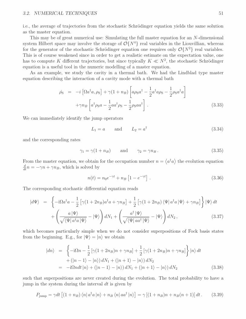
3.2. NUMERICAL TECHNIQUES 51
i.e., the average of trajectories from the stochastic Schrodinger equation yields the same solutionas the master equation.
This may be of great numerical use: Simulating the full master equation for an N -dimensionalsystem Hilbert space may involve the storage of ON4 real variables in the Liouvillian, whereasfor the generator of the stochastic Schrodinger equation one requires only ON2 real variables.This is of course weakened since in order to get a realistic estimate on the expectation value, onehas to compute K different trajectories, but since typically K ≪ N2, the stochastic Schrodingerequation is a useful tool in the numeric modelling of a master equation.
As an example, we study the cavity in a thermal bath. We had the Lindblad type masterequation describing the interaction of a cavity mode with a thermal bath
ρS = −i[Ωa†a, ρS
]+ γ(1 + nB)
[
aρSa† − 1
2a†aρS −
1
2ρSa
†a
]
+γnB
[
a†ρSa−1
2aa†ρS −
1
2ρSaa
†]
. (3.33)
We can immediately identify the jump operators
L1 = a and L2 = a† (3.34)
and the corresponding rates
γ1 = γ(1 + nB) and γ2 = γnB . (3.35)
From the master equation, we obtain for the occupation number n =⟨a†a⟩the evolution equation
ddtn = −γn+ γnB, which is solved by
n(t) = n0e−γt + nB
[1− e−γt
]. (3.36)
The corresponding stochastic differential equation reads
|dΨ〉 =
−iΩa†a− 1
2
[γ(1 + 2nB)a
†a+ γnB
]+
1
2
[γ(1 + 2nB) 〈Ψ| a†a |Ψ〉+ γnB
]
|Ψ〉 dt
+
(
a |Ψ〉√
〈Ψ| a†a |Ψ〉− |Ψ〉
)
dN1 +
(
a† |Ψ〉√
〈Ψ| aa† |Ψ〉− |Ψ〉
)
dN2 , (3.37)
which becomes particularly simple when we do not consider superpositions of Fock basis statesfrom the beginning. E.g., for |Ψ〉 = |n〉 we obtain
|dn〉 =
−iΩn− 1
2[γ(1 + 2nB)n+ γnB] +
1
2[γ(1 + 2nB)n+ γnB]
|n〉 dt
+(|n− 1〉 − |n〉) dN1 + (|n+ 1〉 − |n〉) dN2
= −iΩndt |n〉+ (|n− 1〉 − |n〉) dN1 + (|n+ 1〉 − |n〉) dN2 (3.38)
such that superpositions are never created during the evolution. The total probability to have ajump in the system during the interval dt is given by
Pjump = γdt[(1 + nB) 〈n| a†a |n〉+ nB 〈n| aa† |n〉
]= γ [(1 + nB)n+ nB(n+ 1)] dt . (3.39)

52 CHAPTER 3. SOLVING MASTER EQUATIONS
If no jump occurs, the system evolves only oscillatory, which has no effect on the expectation valueof a†a. However, if a jump occurs, the respective conditional probability to jump out of the systemreads
P1 =(nB + 1)n
(nB + 1)n+ nB(n+ 1)(3.40)
and to jump into the system consequently (these must add up to one)
P2 =nB(n+ 1)
(nB + 1)n+ nB(n+ 1). (3.41)
Computing trajectories with a suitable random number generator and averaging the trajectories,we find convergence to the master equation result as expected, see Fig. 3.2.
0 2 4 6 8 10time γ t
0
2
4
6
8
10
expe
ctat
ion
valu
e <
n(t)
>
master equation solutionaverage of 10 trajectoriesaverage of 100 trajectoriesaverage of 1000 trajectories
Figure 3.2: Single trajectories of the stochastic Schrodinger equation (curves with integer jumps).The averages of 10, 100, and 1000 trajectories converge to the prediction from the associatedmaster equation. Parameters: γdt = 0.01, nB = 1.5.

Chapter 4
Multi-Terminal Coupling :Non-Equilibrium Case I
The most obvious way to achieve non-equilibrium dynamics is to use reservoir states that are non-thermalized, i.e., states that cannot simply be characterized by just temperature and chemicalpotential. Since the derivation of the master equation only requires [ρB,HB] = 0, this would stillallow for many nontrivial models, 〈n| ρB |n〉 could e.g. follow multi-modal distributions. Alterna-tively, a non-equilibrium situation may be established when a system is coupled to different thermalequilibrium baths or of course when the system itself is externally driven – either unconditionally(open-loop feedback) or conditioned on the actual state of the system (closed-loop feedback).
First, we will consider the case of multiple reservoirs at different thermal equilibria that are onlyindirectly coupled via the system: Without the system, they would be completely independent.Since these are chosen at different equilibria, they drag the system towards different thermal states,and the resulting stationary state is in general a non-thermal one. Since the different compartmentsinteract only indirectly via the system, we have the case of a multi-terminal system, where one canmost easily derive the corresponding master equation, since each contact may be treated separately.Therefore, we do now consider multiple (K) reservoirs held at different chemical potentials anddifferent temperatures
ρB =e−β(H(1)
B −µN(1)B )
Tr
e−β(H(1)B −µN
(1)B ) ⊗ . . .⊗ e−β(H(K)
B −µN(K)B )
Tr
e−β(H(K)B −µN
(K)B ) . (4.1)
To each of the reservoirs, the system is coupled via different coupling operators
HI =∑
α
Aα ⊗k∑
ℓ=1
B(ℓ)α . (4.2)
Since we assume that the first order bath correlation functions vanish⟨Bℓ
αρB⟩= 0, the tensor
product implies that the second-order bath correlation functions may be computed additively
Cαβ(τ) =K∑
ℓ=1
C(ℓ)αβ(τ) , (4.3)
which transfers to their Fourier transforms and thus, also to the final Liouvillian (to second order
53

54 CHAPTER 4. MULTI-TERMINAL COUPLING : NON-EQUILIBRIUM CASE I
in the coupling)
L =K∑
ℓ=1
L(ℓ) . (4.4)
The resulting stationary state is in general a non-equilibrium one. Let us however first identify atrivial case where the coupling structure of all Liouvillians is identical
L(ℓ) = Γ(ℓ)[
L0 + β(ℓ)L1
]
, (4.5)
where β(ℓ) is a parameter encoding the thermal properties of the respective bath (e.g. a Fermi-function evaluated at one of the systems transition frequencies) and L0/1 are superoperators inde-pendent of the respective bath and Γ(ℓ) represent different coupling constants. For coupling to asingle reservoir, the stationary state is defined via the equation
L(ℓ)ρ(ℓ) = Γ(ℓ)[
L0 + β(ℓ)L1
]
ρ(ℓ) = 0 (4.6)
and thus implicitly depends on the thermal parameter ρ(ℓ) = ρ(β(ℓ)). For the total Liouvillian, itfollows that the dependence of the full stationary state on all thermal parameters simply given bythe same dependence on an average thermal parameter
∑
ℓ
L(ℓ)ρ =∑
ℓ
Γ(ℓ)[
L0 + β(ℓ)L1
]
ρ =
[∑
ℓ
Γ(ℓ)
][
L0 +
∑
ℓ Γ(ℓ)β(ℓ)
∑
ℓ′ Γ(ℓ′)
L1
]
ρ , (4.7)
such that the dependence is simply ρ = ρ
(∑
ℓ Γ(ℓ)β
(ℓ)
∑ℓ Γ
(ℓ)
)
This can be illustrated by upgrading the Liouvillian for a single resonant level coupled to asingle junction
L =
(−Γf +Γ(1− f)+Γf −Γ(1− f)
)
, (4.8)
where the Fermi function f =[eβ(ǫ−µ) + 1
]−1of the contact is evaluated at the dot level ǫ, to the
Liouvillian for a single-electron transistor (SET) coupled to two (left and right) junctions
L =
(−ΓLfL − ΓRfR +ΓL(1− fL) + ΓR(1− fR)+ΓLfL + ΓRfR −ΓL(1− fL)− ΓR(1− fR)
)
. (4.9)
Now, the system is coupled to two fermionic reservoirs, and in order to support a current, the dotlevel ǫ must be within the transport window, see Fig. 4.1. This also explains the name single-electron transistor, since the dot level ǫ may be tuned by a third gate, which thereby controls thecurrent.
Exercise 29 (Pseudo-Nonequilibrium) (1 points)Show that the stationary state of Eq.(4.9) is a thermal one, i.e., that
ρ11ρ00
=f
1− f.
Determine f in dependence of Γα and fα.

4.1. CONDITIONAL MASTER EQUATION FROM CONSERVATION LAWS 55
Figure 4.1: Sketch of a single resonant level (QD at energy level ǫ) coupled to two junctions withdifferent Fermi distributions (e.g. with different chemical potentials or different temperatures. Ifthe dot level ǫ is changed with a third gate, the device functions as a transistor, since the currentthrough the system is exponentially suppressed when the the dot level ǫ is not within the transportwindow.
4.1 Conditional Master equation from conservation laws
Suppose we have derived a QME for an open system, where the combined system obeys theconservation of some conserved quantity (e.g., the total number of particles). Then, it can bedirectly concluded that a change in the system particle number by e.g. minus one must be directlyaccompagnied by the corresponding change of the reservoir particle number by plus one. Forcouplings to multiple reservoirs these terme can also be uniquely identified, since the Liouvilliansare additive. Whereas its actual density matrix says little about the number of quanta that havealready passed the quantum system, a full trajectory would reveal this information. In such cases,it is reasonable to discretize the master equation in time, where it can most easily be upgraded toan n-resolved (conditional) master equation. In what follows, we just track the particle number ina single attached reservoir and denote by ρ(n)(t) the system density matrix under the condition thatn net particles have left into the monitored reservoirs, but the method may easily be generalized.Assuming that at time t, we have n particles transferred to the reservoir, we may discretize theconventional master equation ρ = Lρ in time and identify terms that increase or decrease theparticle number (often called jumpers)
˙ρ(n) = L0ρ(n) + L+ρ(n−1) + L−ρ(n+1) . (4.10)
Since the total number of transferred particles is normally not constrained, this immediately yieldsan infinite set of equations for the system density matrix. Exploiting the translational invariancesuggests to use the Fourier transform
ρ(χ, t) =∑
n
ρ(n)(t)e+inχ , (4.11)
which again reduces the dimension of the master equation
ρ(χ, t) =[L0 + e+iχL+ + e−iχL−] ρ(χ, t) = L(χ)ρ(χ, t) . (4.12)
As an example, we convert the SET master equation (4.9) into an n-resolved version, where n
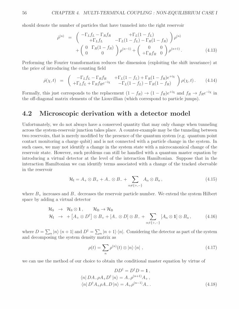
56 CHAPTER 4. MULTI-TERMINAL COUPLING : NON-EQUILIBRIUM CASE I
should denote the number of particles that have tunneled into the right reservoir
ρ(n) =
(−ΓLfL − ΓRfR +ΓL(1− fL)
+ΓLfL −ΓL(1− fL)− ΓR(1− fR)
)
ρ(n)
+
(0 ΓR(1− fR)0 0
)
ρ(n−1) +
(0 0
+ΓRfR 0
)
ρ(n+1) . (4.13)
Performing the Fourier transformation reduces the dimension (exploiting the shift invariance) atthe price of introducing the counting field
ρ(χ, t) =
(−ΓLfL − ΓRfR +ΓL(1− fL) + ΓR(1− fR)e
+iχ
+ΓLfL + ΓRfRe−iχ −ΓL(1− fL)− ΓR(1− fR)
)
ρ(χ, t) . (4.14)
Formally, this just corresponds to the replacement (1 − fR) → (1 − fR)e+iχ and fR → fRe
−iχ inthe off-diagonal matrix elements of the Liouvillian (which correspond to particle jumps).
4.2 Microscopic derivation with a detector model
Unfortunately, we do not always have a conserved quantity that may only change when tunnelingacross the system-reservoir junction takes place. A counter-example may be the tunneling betweentwo reservoirs, that is merely modified by the presence of the quantum system (e.g. quantum pointcontact monitoring a charge qubit) and is not connected with a particle change in the system. Insuch cases, we may not identify a change in the system state with a microcanonical change of thereservoir state. However, such problems can still be handled with a quantum master equation byintroducing a virtual detector at the level of the interaction Hamiltonian. Suppose that in theinteraction Hamiltonian we can identify terms associated with a change of the tracked obervablein the reservoir
HI = A+ ⊗B+ + A− ⊗B− +∑
α 6=+,−Aα ⊗ Bα , (4.15)
where B+ increases and B− decreases the reservoir particle number. We extend the system Hilbertspace by adding a virtual detector
HS → HS ⊗ 1 , HB → HB
HI → +[A+ ⊗D†]⊗B+ + [A− ⊗D]⊗ B− +
∑
α 6=+,−[Aα ⊗ 1]⊗Bα , (4.16)
where D =∑
n |n〉 〈n+ 1| and D† =∑
n |n+ 1〉 〈n|. Considering the detector as part of the systemand decomposing the system density matrix as
ρ(t) =∑
n
ρ(n)(t)⊗ |n〉 〈n| , (4.17)
we can use the method of our choice to obtain the conditional master equation by virtue of
DD† = D†D = 1 ,
〈n|DA−ρA+D† |n〉 = A−ρ
(n+1)A+ ,
〈n|D†A+ρA−D |n〉 = A+ρ(n−1)A− . (4.18)

4.3. FULL COUNTING STATISTICS 57
4.3 Full Counting Statistics
To obtain the probability of having n tunneled particles into a respective reservoir, we have to sumover the different system configurations of the corresponding conditional density matrix
Pn(t) = Trρ(n)(t)
. (4.19)
In view of the identities
Tr ρ(χ, t) = TreL(χ)tρ0
=∑
n
Pn(t)e+inχ ≡ M(χ, t) , (4.20)
we see that in order to evaluate moments⟨nk⟩, we simply have to take derivatives with respect to
the counting field
⟨nk(t)
⟩=∑
n
nkPn(t) = (−i∂χ)k∑
n
Pn(t)e+inχ
∣∣∣∣∣χ=0
= (−i∂χ)k M(χ, t)|χ=0 . (4.21)
Based on a conditional master equation, this enables a very convenient calculation of the stationarycurrent. Taking the stationary density matrix L(0)ρ = 0 as initial condition (the stationary currentis independent on the initial occupation of the density matrix), we obtain for the current as thetime derivative of the first moment
I = 〈n(t)〉
= −i∂χd
dtTreL(χ)tρ
∣∣χ=0
= −i∂χ TrL(χ)eL(χ)tρ
∣∣χ=0
= −iTr
L′(0)ρ+ [L′(0)L(0) + L(0)L′(0)] tρ
+[L′(0)L2(0) + L(0)L′(0)L(0) + L2(0)L′(0)
] t2
2ρ+ . . .
= −iTr L′(0)ρ , (4.22)
where we have used L(0)ρ = 0 and also Tr L(0)σ = 0 for all operators σ (trace conservation).
Exercise 30 (Stationary SET current) (1 points)Calculate the stationary current through the SET (4.14).
Sometimes a description in terms of cumulants is more convenient. The cumulant-generatingfunction is defined as the logarithm of the moment-generating function
C(χ, t) = lnM(χ, t) , (4.23)
such that all cumulants may be obtained via simple differentiation
⟨⟨nk⟩⟩
= (−i∂χ)k C(χ, t)|χ=0 . (4.24)

58 CHAPTER 4. MULTI-TERMINAL COUPLING : NON-EQUILIBRIUM CASE I
Cumulants and Moments are of course related, we just summarize relations for the lowest fewcumulants
〈〈n〉〉 = 〈n〉 ,⟨⟨n2⟩⟩
=⟨n2⟩− 〈n〉2 ,
⟨⟨n3⟩⟩
=⟨n3⟩− 3 〈n〉
⟨n2⟩+ 2 〈n〉3 ,
⟨⟨n4⟩⟩
=⟨n4⟩− 4 〈n〉
⟨n3⟩− 3
⟨n2⟩2
+ 12 〈n〉2⟨n2⟩− 6 〈n〉4 . (4.25)
The advantage of this description lies in the fact that the long-term evolution of the cumulant-generating function is usually given by the dominant eigenvalue of the Liouvillian
C(χ, t) ≈ λ(χ)t , (4.26)
where λ(χ) is the (uniqueness assumed) eigenvalue of the Liouvillian that vanishes at zero countingfield λ(0) = 0. For this reason, the dominant eigenvalue is also interpreted as the cumulant-generating function of the stationary current.
Exercise 31 (current CGF for the SET) (1 points)Calculate the dominant eigenvalue of the SET Liouvillian (4.14) in the infinite bias limit fL → 1and fR → 0. What is the value of the current?
We show this by using the decomposition of the Liouvillian in Jordan Block form
L(χ) = Q(χ)LJ(χ)Q−1(χ) , (4.27)
where Q(χ) is a (non-unitary) similarity matrix and LJ(χ) contains the eigenvalues of the Liouvil-lian on its diagonal – distributed in blocks with a size corresponding to the eigenvalue multiplicity.We assume that there exists one stationary state ρ, i.e., one eigenvalue λ(χ) with λ(0) = 0 and thatall other eigenvalues have a larger negative real part near χ = 0. Then, we use this decompositionin the matrix exponential to estimate its long-term evolution
M(χ, t) = TreL(χ)tρ0
= Tr
eQ(χ)LJ (χ)Q−1(χ)tρ0
= TrQ(χ)eLJ (χ)tQ−1(χ)ρ0
→ Tr
Q(χ)
eλ(χ)·t
0. . .
0
Q−1(χ)ρ0
= eλ(χ)·tTr
Q(χ)
10
. . .
0
Q−1(χ)ρ0
= eλ(χ)tc(χ) (4.28)
with some polynomial c(χ) depending on the matrix Q(χ). This implies that the cumulant-generating function
C(χ, t) = lnM(χ, t) = λ(χ)t+ ln c(χ) ≈ λ(χ)t (4.29)
becomes linear in λ(χ) for large times.

4.4. FLUCTUATION THEOREMS 59
4.4 Fluctuation Theorems
The probability distribution Pn(t) is given by the inverse Fourier transform of the moment-generating function
Pn(t) =1
2π
+π∫
−π
M(χ, t)e−inχdχ =1
2π
+π∫
−π
eC(χ,t)−inχdχ . (4.30)
Accordingly, a symmetry in the cumulant-generating function (or moment-generating function) ofthe form
C(−χ, t) = C(+χ+ i ln(α), t) (4.31)
leads to a symmetry of the probabilities
P+n(t)
P−n(t)=
12π
∫ +π
−πeC(χ,t)−inχdχ
12π
∫ +π
−πeC(χ,t)+inχdχ
=
∫ +π
−πeC(χ,t)−inχdχ
∫ +π
−πeC(−χ,t)−inχdχ
=
∫ +π
−πeC(χ,t)−inχdχ
∫ +π
−πeC(χ+i ln(α),t)−inχdχ
=
∫ +π
−πeC(χ,t)−inχdχ
∫ +π+i ln(α)
−π+i ln(α)eC(χ,t)−in[χ−i ln(α)]dχ
= e+n ln(α) , (4.32)
where we have used in the last step that C(−π + i ln(α), t) = C(+π + i ln(α), t), such that wecan add two further integration paths from −π to −π + i ln(α) and from +π + i ln(α) to +π.The value of the cumulant-generating function along these paths is the same, such that due tothe different integral orientation there is not net change. Note that the system may be very farfrom thermodynamic equilibrium but still obey a symmetry of the form (4.31), which leads to afluctuation theorem of the form (4.32) being valid far from equilibrium.
As example, we consider the SET (which is always in thermal equilibrium). The characteristicpolynomial D(χ) = |L(χ)− λ1| of the Liouvillian (4.14) and therefore also all eigenvalues obeysthe symmetry
D(−χ) = D(
+χ+ i ln
[fL(1− fR)
(1− fL)fR
])
= D (χ+ i [(βR − βL) ǫ+ βLµL − βRµR]) , (4.33)
which leads to the fluctuation theorem
limt→∞
P+n(t)
P−n(t)= en[(βR−βL)ǫ+βLµL−βRµR] . (4.34)
For equal temperatures, this becomes
limt→∞
P+n(t)
P−n(t)= enβV , (4.35)
which directly demonstrates that the current
I =d
dt〈n(t)〉 = d
dt
+∞∑
n=−∞nPn(t) =
∞∑
n=1
n [P+n(t)− P−n(t)] =∞∑
n=1
nPn(t)[1− e−nα
](4.36)
always follows the voltage.

60 CHAPTER 4. MULTI-TERMINAL COUPLING : NON-EQUILIBRIUM CASE I
4.5 The double quantum dot
We consider a double quantum dot with internal tunnel coupling T and Coulomb interaction Uthat is weakly coupled to two fermionic contacts via the rates ΓL and ΓR, see Fig. 4.2. The
Figure 4.2: A double quantum dot (system) with on-site energies ǫA/B and internal tunnelingamplitude T and Coulomb interaction U may host at most two electrons. It is weakly tunnel-coupled to two fermionic contacts via the rates ΓL/R at different thermal equilibria described bythe Fermi distributions fL/R(ω).
corresponding Hamiltonian reads
HS = ǫAd†AdA + ǫBd
†BdB + T
(
dAd†B + dBd
†A
)
+ Ud†AdAd†BdB ,
HB =∑
k
ǫkLc†kLckL +
∑
k
ǫkRc†kRckR ,
HI =∑
k
(
tkLdAc†kL + t∗kLckLd
†A
)
+∑
k
(
tkRdBc†kR + t∗kRckRd
†B
)
. (4.37)
Note that we do not have a tensor product decomposition in the interaction Hamiltonian, as thecoupling operators anti-commute, e.g.,
d, ckR = 0 . (4.38)
We may however use the Jordan Wigner transform, which decomposes the Fermionic operators interms of Pauli matrices acting on different spins
dA = σ− ⊗ 1⊗ 1⊗ . . .⊗ 1 , dB = σz ⊗ σ− ⊗ 1⊗ . . .⊗ 1 ,
ckL = σz ⊗ σz ⊗ σz ⊗ . . .⊗ σz
︸ ︷︷ ︸
k−1
⊗σ− ⊗ 1⊗ . . .⊗ 1 ,
ckR = σz ⊗ σz ⊗ σz ⊗ . . .⊗ σz
︸ ︷︷ ︸
KL
⊗ σz ⊗ . . .⊗ σz
︸ ︷︷ ︸
k−1
⊗σ− ⊗ 1⊗ . . .⊗ 1 (4.39)
to map to a tensor-product decomposition of the interaction Hamiltonian, where σ± = 12[σx ± iσy].
The remaining operators follow from (σ+)†= σ− and vice versa. This decomposition automat-
ically obeys the fermionic anti-commutation relations such as e.g.ck, d
† = 0 and may there-fore also be used to create a fermionic operator basis with computer algebra programs (e.g. useKroneckerProduct in Mathematica).

4.5. THE DOUBLE QUANTUM DOT 61
Exercise 32 (Jordan-Wigner transform) (1 points)Show that for fermions distributed on N sites, the decomposition
ci = σz ⊗ . . .⊗ σz
︸ ︷︷ ︸
i−1
⊗σ− ⊗ 1⊗ . . .⊗ 1︸ ︷︷ ︸
N−i
preserves the fermionic anti-commutation relations
ci, cj = 0 =
c†i , c†j
,
ci, c†j
= δij1 .
Show also that the fermionic Fock space basis c†ici |n1, . . . , nN〉 = ni |n1, . . . , nN〉 obeysσzi |n1, . . . , nN〉 = (−1)ni+1 |n1, . . . , nN〉.
Inserting the decomposition (4.39) in the Hamiltonian, we may simply use the relations
(σx)2 = (σy)2 = (σz)2 = 1 , σ+σ− =1
2[1+ σz] , σ−σ+ =
1
2[1− σz] ,
σzσ− = −σ− , σ−σz = +σ− , σzσ+ = +σ+ , σ+σz = −σ+ (4.40)
to obtain a system of interacting spins
HS = ǫA1
2[1+ σz
A] + ǫB1
2[1+ σz
B] + T[σ−Aσ
+B + σ+
Aσ−B
]+ U
1
2[1+ σz
A]1
2[1+ σz
B]
HB =∑
k
ǫkL1
2[1+ σz
kL] +∑
k
ǫkR1
2[1+ σz
kR]
HI = σ−Aσ
zB ⊗
∑
k
tkL
[∏
k′<k
σzk′L
]
σ+kL + σ+
AσzB ⊗
∑
k
t∗kL
[∏
k′<k
σzk′L
]
σ−kL
+σ−B ⊗
∑
k
tkR
[∏
k′
σzk′L
][∏
k′′<k
σzk′′R
]
σ+kR + σ+
B ⊗∑
k
t∗kR
[∏
k′
σzk′L
][∏
k′′<k
σzk′′R
]
σ−kR
. (4.41)
With this, we could proceed by simply viewing the Hamiltonian as a complicated total systemof non-locally interacting spins. However, the order of operators in the nonlocal Jordan-Wignertransformation may be chosen as convenient without destroying the fermionic anticommutationrelations. We may therefore also define new fermionic operators on the subspace of the system (firsttwo sites, with reversed order) and the baths (all remaining sites with original order), respectively
dA = σ− ⊗ σz , dB = 1⊗ σ− ,
ckL = σz ⊗ . . .⊗ σz
︸ ︷︷ ︸
k−1
⊗σ− ⊗ 1⊗ . . .⊗ 1 ,
ckR = σz ⊗ . . .⊗ σz
︸ ︷︷ ︸
KL
⊗ σz ⊗ . . .⊗ σz
︸ ︷︷ ︸
k−1
⊗σ− ⊗ 1⊗ . . .⊗ 1 . (4.42)
These new operators obey fermionic anti-commutation relations in system and bath separately(e.g. dA, dB = 0 and ckL, ck′L = 0), but act on different Hilbert spaces, such that system and

62 CHAPTER 4. MULTI-TERMINAL COUPLING : NON-EQUILIBRIUM CASE I
bath operators do commute by construction (e.g. [dA, ckL] = 0). In the new operator basis, theHamiltonian appears as
HS =[
ǫAd†AdA + ǫBd
†BdB + T
(
dAd†B + dBd
†A
)
+ Ud†AdAd†BdB
]
⊗ 1 ,
HB = 1⊗[∑
k
ǫkLc†kLckL +
∑
k
ǫkRc†kRckR
]
,
HI = dA ⊗∑
k
tkLc†kL + d†A ⊗
∑
k
t∗kLckL + dB ⊗∑
k
tkRc†kR + d†B ⊗
∑
k
t∗kRckR , (4.43)
which is the same (for this and some more special cases) as if we had ignored the fermionic natureof the annihilation operators from the beginning. We do now proceed by calculating the Fouriertransforms of the bath correlation functions
γ12(ω) = ΓL(−ω)fL(−ω) , γ21(ω) = ΓL(+ω)[1− fL(+ω)] ,
γ34(ω) = ΓR(−ω)fR(−ω) , γ43(ω) = ΓR(+ω)[1− fR(+ω)] (4.44)
with the continuum tunneling rates Γα(ω) = 2π∑
k |tkα|2δ(ω− ǫkα) and Fermi functions fα(ǫkα) =⟨
c†kαckα
⟩
.
Exercise 33 (DQD bath correlation functions) (1 points)Calculate the Fourier transforms (4.44) of the bath correlation functions for the double quantumdot.
Next, we diagonalize the system Hamiltonian (in the Fock space basis)
E0 = 0 , |v0〉 = |00〉 ,E− = ǫ−
√∆2 + T 2 , |v−〉 ∝
[(
∆+√∆2 + T 2
)
|10〉+ T |01〉]
,
E+ = ǫ+√∆2 + T 2 , |v+〉 ∝
[(
∆−√∆2 + T 2
)
|10〉+ T |01〉]
,
E2 = 2ǫ+ U , |v2〉 = |11〉 , (4.45)
where ∆ = (ǫB − ǫA)/2 and ǫ = (ǫA + ǫB)/2 and |01〉 = −d†B |00〉, |10〉 = d†A |00〉, and |11〉 =d†Bd
†A |00〉. We have not symmetrized the coupling operators but to obtain the BMS limit, we may
alternatively use Eqns. (2.60) and (2.61) when τ → ∞ . Specifically, when we have no degeneraciesin the system Hamiltonian (∆2 + T 2 > 0), the master equation in the energy eigenbasis (wherea, b ∈ 0,−,+, 2) becomes a rate equation ρaa = +
∑
b γab,abρbb − [∑
b γba,ba] ρaa with the ratecoefficients
γab,ab =∑
αβ
γαβ(Eb − Ea) 〈a|Aβ |b〉 〈a|A†α |b〉∗ . (4.46)
We may calculate the Liouvillians for the interaction with the left and right contact separately
γab,ab = γLab,ab + γR
ab,ab , (4.47)

4.5. THE DOUBLE QUANTUM DOT 63
since we are constrained to second order perturbation theory in the tunneling amplitudes. Sincewe have dA = A†
2 = A1 = dA and dB = A†4 = A2 = dB, we obtain for the left-associated dampening
coefficients
γLab,ab = γ12(Eb − Ea)|〈a|A2 |b〉|2 + γ21(Eb − Ea)|〈a|A1 |b〉|2 ,
γRab,ab = γ34(Eb − Ea)|〈a|A4 |b〉|2 + γ43(Eb − Ea)|〈a|A3 |b〉|2 . (4.48)
In the wideband (flatband) limit ΓL/R(ω) = ΓL/R, we obtain for the nonvanishing transition ratesin the energy eigenbasis
γL0−,0− = ΓLγ+[1− fL(ǫ−
√∆2 + T 2)] , γR
0−,0− = ΓRγ−[1− fR(ǫ−√∆2 + T 2)] ,
γL0+,0+ = ΓLγ−[1− fL(ǫ+
√∆2 + T 2)] , γR
0+,0+ = ΓRγ+[1− fR(ǫ+√∆2 + T 2)] ,
γL−2,−2 = ΓLγ−[1− fL(ǫ+ U +
√∆2 + T 2)] , γR
−2,−2 = ΓRγ+[1− fR(ǫ+ U +√∆2 + T 2)] ,
γL+2,+2 = ΓLγ+[1− fL(ǫ+ U −
√∆2 + T 2)] , γR
+2,+2 = ΓRγ−[1− fR(ǫ+ U −√∆2 + T 2)] ,
γL−0,−0 = ΓLγ+fL(ǫ−
√∆2 + T 2) , γR
−0,−0 = ΓRγ−fR(ǫ−√∆2 + T 2) ,
γL+0,+0 = ΓLγ−fL(ǫ+
√∆2 + T 2) , γR
+0,+0 = ΓRγ+fR(ǫ+√∆2 + T 2) ,
γL2−,2− = ΓLγ−fL(ǫ+ U +
√∆2 + T 2) , γR
2−,2− = ΓRγ+fR(ǫ+ U +√∆2 + T 2) ,
γL2+,2+ = ΓLγ+fL(ǫ+ U −
√∆2 + T 2) , γR
2+,2+ = ΓRγ−fR(ǫ+ U −√∆2 + T 2) , (4.49)
with the dimensionless coefficients
γ± =1
2
[
1± ∆√∆2 + T 2
]
(4.50)
arising from the matrix elements of the system coupling operators. This rate equation can also bevisualized with a network, see Fig. 4.3.
Figure 4.3: Configuration space of a serialdouble quantum dot coupled to two leads.Due to the hybridization of the two levels,electrons may jump directly from the leftcontact to right-localized modes and viceversa, such that in principle all transitios aredriven by both contacts. However, the rel-ative strength of the couplings is different,such that the two Liouillians have a differentstructure. In the Coulomb-blockade limit,transitions to the doubly occupied state areforbidden (dotted lines), such that the sys-tem dimension can be reduced.
As the simplest example of the resulting rate equation, we study the high-bias and Coulomb-blockade limit fL/R(ǫ+U±
√∆2 + T 2) → 0 and fL(ǫ±
√∆2 + T 2) → 1 and fR(ǫ±
√∆2 + T 2) → 0
when ∆ → 0 (such that γ± → 1/2). This removes any dependence on T and therefore, a currentwill be predicted even when T → 0 (where we have a disconnected structure). However, precisely in

64 CHAPTER 4. MULTI-TERMINAL COUPLING : NON-EQUILIBRIUM CASE I
this limit, the two levels E− and E+ become energetically degenerate, such that we cannot neglectthe couplings to the coherences anymore and the BMS limit is not applicable. The resultingLiouvillian reads
L =1
2
−2ΓL ΓR ΓR 0ΓL −ΓR 0 ΓL + ΓR
ΓL 0 −ΓR ΓL + ΓR
0 0 0 −2(ΓL + ΓR)
, (4.51)
where it becomes visible that the doubly occupied state will simply decay and may therefore –since we are interested in the long-term dynamics – be eliminated completely
LCBHB =1
2
−2ΓL ΓR ΓR
ΓL −ΓR 0ΓL 0 −ΓR
. (4.52)
Switching to a conditional Master equation by counting all electrons in the right junction andperforming the Fourier summation corresponds formally to the replacement ΓR → ΓRe
+iχ in alloff-diagonal matrix elements (corresponding to single-electron jumps), such that we have
LCBHB(χ) =1
2
−2ΓL ΓRe+iχ ΓRe
+iχ
ΓL −ΓR 0ΓL 0 −ΓR
. (4.53)
Exercise 34 (Stationary Current) (1 points)Calculate the stationary current of Eq.(4.53).
Exercise 35 (Nonequilibrium Stationary State) (1 points)Show that the stationary state of Eq. (4.52) cannot be written as a grand-canonical equilibriumstate by disproving the equations ρ−−/ρ00 = e−β(E−−E0−µ), ρ++/ρ00 = e−β(E+−E0−µ) and ρ++/ρ−− =e−β(E+−E−)

Chapter 5
Direct bath coupling :Non-Equilibrium Case II
Another nonequilibrium situation may be generated by a multi-component bath with componentsinteracting directly (i.e., even without the presence of the system) via a small interface. However,the interaction may be modified by the presence of the quantum system. A prototypical examplefor such a bath is a quantum point contact: The two leads are held at different potentials andthrough a tiny contact charges may tunnel. The tunneling process is however highly sensitive tothe presence of nearby charges, in the Hamiltonian this is modeled by a capacitive change of thetunneling amplitudes. When already the baseline tunneling amplitudes (in a low transparencyQPC) are small, we may apply the master equation formalism without great efforts, as will bedemonstrated at two examples.
5.1 Monitored SET
High-precision tests of counting statistics have been performed with a quantum point contact thatis capacitively coupled to a single-electron transistor. The Hamiltonian of the system depicted inFig. 5.1 reads
Figure 5.1: Sketch of a quantum point contact (in fact, a two component bath with the componentsheld at different chemical potential) monitoring a single electron transistor. The tunneling throughthe quantum point contact is modified when the SET is occupied.
65

66 CHAPTER 5. DIRECT BATH COUPLING : NON-EQUILIBRIUM CASE II
HS = ǫd†d ,
HB =∑
k
ǫkLc†kLckL +
∑
k
ǫkLc†kRckR +
∑
k
εkLγ†kLγkL +
∑
k
εkLγ†kRγkR ,
HI =
[∑
k
tkLdc†kL +
∑
k
tkRdc†kR + h.c.
]
+
[∑
kk′
(tkk′ + d†dτkk′
)γkLγ
†k′R + h.c.
]
, (5.1)
where ǫ denotes the dot level, ckα annihilate electrons on SET lead α and γkα are the annihilationoperators for the QPC lead α. The QPC baseline tunneling amplitude is given by tkk′ and describesthe scattering of and electron from mode k in the left lead to mode k′ in the right QPC contact.When the nearby SET is occupied it is modified to tkk′ + τkk′ , where τkk′ represents the change ofthe tunneling amplitude.
We will derive a master equation for the dynamics of the SET due to the interaction with theQPC and the two SET contacts. In addition, we are interested not only in the charge countingstatistics of the SET but also the QPC. The Liouvillian for the SET-contact interaction is wellknown and has been stated previously (we insert counting fields at the right lead)
LSET(χ) =
(−ΓLfL − ΓRfR +ΓL(1− fL) + ΓR(1− fR)e
+iχ
+ΓLfL + ΓRfRe−iχ −ΓL(1− fL)− ΓR(1− fR)
)
. (5.2)
We will therefore derive the dissipator for the SET-QPC interaction separately. To keep trackof the tunneled QPC electrons, we insert a virtual detector operator in the respective tunnelingHamiltonian
HQPCI =
∑
kk′
(tkk′1+ d†dτkk′
)B†γkLγ
†k′R +
∑
kk′
(t∗kk′1+ d†dτ ∗kk′
)Bγk′Rγ
†kL
= 1⊗B† ⊗∑
kk′
tkk′γkLγ†k′R + 1⊗B ⊗
∑
kk′
t∗kk′γk′Rγ†kL
+d†d⊗B† ⊗∑
kk′
τkk′γkLγ†k′R + d†d⊗B ⊗
∑
kk′
τ ∗kk′γk′Rγ†kL . (5.3)
Note that we have implicitly performed the mapping to a tensor product representation of thefermionic operators, which is unproblematic here as between SET and QPC no particle exchangetakes place and the electrons in the QPC and the SET may be treated as different particle types.To simplify the system, we assume that the change of tunneling amplitudes affects all modes inthe same manner, i.e., τkk′ = τ tkk′ , which enables us to combine some coupling operators
HQPCI =
[1+ τ d†d
]⊗B† ⊗
∑
kk′
tkk′γkLγ†k′R +
[1+ τ ∗d†d
]⊗B ⊗
∑
kk′
t∗kk′γk′Rγ†kL . (5.4)
The evident advantage of this approximation is that only two correlation functions have to becomputed. We can now straightforwardly (since the baseline tunneling term is not included in thebath Hamiltonian) map to the interaction picture
B1(τ) =∑
kk′
tkk′γkLγ†k′Re
−i(εkL−εk′R)τ , B2(τ) =∑
kk′
t∗kk′γk′Rγ†kLe
+i(εkL−εk′R)τ . (5.5)

5.1. MONITORED SET 67
For the first bath correlation function we obtain
C12(τ) =∑
kk′
∑
ℓℓ′
tkk′t∗ℓℓ′e
−i(εkL−εk′R)τ⟨
γkLγ†k′Rγℓ′Rγ
†ℓL
⟩
=∑
kk′
|tkk′|2e−i(εkL−εk′R)τ [1− fL(εkL)] fR(εk′R)
=1
2π
∫ ∫
T (ω, ω′) [1− fL(ω)] fR(ω′)e−i(ω−ω′)τdωdω′ , (5.6)
where we have introduced T (ω, ω′) = 2π∑
kk′ |tkk′|2δ(ω − εkL)δ(ω − εk′R). Note that in contrast
to previous tunneling rates, this quantity is dimensionless. The integral factorizes when T (ω, ω′)factorizes (or when it is flat T (ω, ω′) = t). In this case, the correlation function C12(τ) is expressedas a product in the time domain, such that its Fourier transform will be given by a convolutionintegral
γ12(Ω) =
∫
C12(τ)e+iΩτdτ
= t
∫
dωdω′ [1− fL(ω)] fR(ω′)δ(ω − ω′ − Ω)
= t
∫
[1− fL(ω)] fR(ω − Ω)dω . (5.7)
For the other correlation function, we have
γ21(Ω) = t
∫
fL(ω) [1− fR(ω + Ω)] dω . (5.8)
Exercise 36 (Correlation functions for the QPC) (1 points)Show the validity of Eqns. (5.8).
The structure of the Fermi functions demonstrates that the shift Ω can be included in thechemical potentials. Therefore, we consider integrals of the type
I =
∫
f1(ω) [1− f2(ω)] dω . (5.9)
At zero temperature, these should behave as I ≈ (µ1 − µ2)Θ(µ1 − µ2), where Θ(x) denotes theHeaviside-Θ function, which follows from the structure of the integrand, see Fig. 5.2. For finitetemperatures, the value of the integral can also be calculated, for simplicity we constrain ourselvesto the (experimentally relevant) case of equal temperatures (β1 = β2 = β), for which we obtain
I =
∫1
(eβ(µ2−ω) + 1) (e−β(µ1−ω) + 1)dω
= limδ→∞
∫1
(eβ(µ2−ω) + 1) (e−β(µ1−ω) + 1)
δ2
δ2 + ω2dω , (5.10)

68 CHAPTER 5. DIRECT BATH COUPLING : NON-EQUILIBRIUM CASE II
0
0,5
1
µ2 µ1
f1(ω)[1-f
2(ω)]
f1(ω)
1-f2(ω)
kB T
2k
B T
1
Figure 5.2: Integrand in Eq. (5.9). At zerotemperature at both contacts, we obtain aproduct of two step functions and the areaunder the curve is given by the differenceµ1 − µ2 as soon as µ1 > µ2 (and zero other-wise).
where we have introduced the Lorentzian-shaped regulator to enforce convergence. By identifyingthe poles of the integrand
ω∗± = ±iδ ,
ω∗1,n = µ1 +
π
β(2n+ 1)
ω∗2,n = µ2 +
π
β(2n+ 1) (5.11)
where n ∈ 0,±1,±2,±3, . . . we can solve the integral by using the residue theorem, see alsoFig. 5.3 for the integration contour. Finally, we obtain for the integral
Figure 5.3: Poles and integration contour forEq. (5.9) in the complex plane. The integralalong the real axis (blue line) closed by anarc (red curve) in the upper complex plane,along which (due to the regulator) the inte-grand vanishes sufficiently fast.
I = 2πi limδ→∞
Res f1(ω) [1− f2(ω)]δ2
δ2 + ω2
∣∣∣∣ω=+iδ
+∞∑
n=0
Res f1(ω) [1− f2(ω)]δ2
δ2 + ω2
∣∣∣∣ω=µ1+
πβ(2n+1)
+∞∑
n=0
Res f1(ω) [1− f2(ω)]δ2
δ2 + ω2
∣∣∣∣ω=µ2+
πβ(2n+1)
=µ1 − µ2
1− e−β(µ1−µ2), (5.12)
which automatically obeys the simple zero-temperature (β → ∞) limit. With the replacements

5.1. MONITORED SET 69
µ1 → µR + Ω and µ2 → µL, we obtain for the first bath correlation function
γ12(Ω) = tΩ− V
1− e−β(Ω−V ), (5.13)
where V = µL − µR is the QPC bias voltage. Likewise, with the replacements µ1 → µL andµ2 → µR − Ω, the second bath correlation function becomes
γ21(Ω) = tΩ + V
1− e−β(Ω+V ). (5.14)
Now we can calculate the transition rates in our system (containing the virtual detector and thequantum dot) for a non-degenerate system spectrum. However, now the detector is part of oursystem. Therefore, the system state is not only characterized by the number of charges on theSET dot a ∈ 0, 1 but also by the number of charges n that have tunneled through the QPC andhave thereby changed the detector state
ρ(a,n)(a,n) =∑
b,m
γ(a,n)(b,m),(a,n)(b,m)ρ(b,m)(b,m) −[∑
b,m
γ(b,m)(a,n),(b,m)(a,n)
]
ρ(a,n)(a,n) . (5.15)
Shortening the notation by omitting the double-indices we may also write
ρ(n)aa =∑
b,m
γ(a,n),(b,m)ρ(m)bb −
[∑
b,m
γ(b,m),(a,n)
]
ρ(n)aa , (5.16)
where ρ(n)aa = ρ(a,n),(a,n) and γ(a,n),(b,m) = γ(a,n)(a,n),(b,m)(b,m). It is evident that the coupling operators
A1 = (1 + τ d†d) ⊗ B† and A2 = (1 + τ ∗d†d) ⊗ B only allow for sequential tunneling through theQPC at lowest order (i.e., m = n ± 1) and do not induce transitions between different dot states(i.e., a = b), such that the only non-vanishing contributions may arise for
γ(0,n)(0,n+1) = γ12(0) 〈0, n|A2 |0, n+ 1〉 〈0, n|A†1 |0, n+ 1〉∗ = γ12(0) ,
γ(0,n)(0,n−1) = γ21(0) 〈0, n|A1 |0, n− 1〉 〈0, n|A†2 |0, n− 1〉∗ = γ21(0) ,
γ(1,n)(1,n+1) = γ12(0) 〈1, n|A2 |1, n+ 1〉 〈1, n|A†1 |1, n+ 1〉∗ = γ12(0)|1 + τ |2 ,
γ(1,n)(1,n−1) = γ21(0) 〈1, n|A1 |1, n− 1〉 〈1, n|A†2 |1, n− 1〉∗ = γ21(0)|1 + τ |2 . (5.17)
The remaining terms just account for the normalization.
Exercise 37 (Normalization terms) (1 points)Compute the remaining rates
∑
m
γ(0,m)(0,m),(0,n)(0,n) , and∑
m
γ(1,m)(1,m),(1,n)(1,n)
explicitly.

70 CHAPTER 5. DIRECT BATH COUPLING : NON-EQUILIBRIUM CASE II
Adopting the notation of conditional master equations, this leads to the connected system
ρ(n)00 = γ12(0)ρ
(n+1)00 + γ21(0)ρ
(n−1)00 − [γ12(0) + γ21(0)] ρ
(n)00
ρ(n)11 = |1 + τ |2γ12(0)ρ(n+1)
11 + |1 + τ |2γ21(0)ρ(n−1)11 − |1 + τ |2 [γ12(0) + γ21(0)] ρ
(n)11 , (5.18)
such that after Fourier transformation with the counting field ξ for the QPC, we obtain thefollowing dissipator
LQPC(ξ) =
( [γ21(e+iχ − 1
)+ γ12
(e−iχ − 1
)]0
0 |1 + τ |2[γ21(e+iχ − 1
)+ γ12
(e−iχ − 1
)]
)
,
(5.19)
which could not have been deduced directly from a Liouvillian for the SET alone. More closelyanalyzing the Fourier transforms of the bath correlation functions
γ21 = γ21(0) = tV
1− e−βV,
γ12 = γ12(0) = tV
e+βV − 1(5.20)
we see that for sufficiently large QPC bias voltages, transport becomes unidirectional and only onecontribution remains and the other one is exponentially suppressed. The sum of both Liouvillians(5.2) and (5.19) constitutes the total dissipator
L(χ, ξ) = LSET(χ) + LQPC(ξ) , (5.21)
which can be used to calculate the probability distributions for tunneling through both transportchannels (QPC and SET).
Exercise 38 (QPC current) (1 points)Show that the stationary state of the SET is unaffected by the additional QPC dissipator andcalculate the stationary current through the QPC for Liouvillian (5.21).
When we consider the case ΓL,ΓR ≪ tV, |1 + τ |tV , we approach a bistable system, andthe counting statistics approaches the case of telegraph noise. When the dot is empty or filledthroughout respectively, the current can easily be determined as
I0 = [γ21(0)− γ12(0)] , I1 = |1 + τ |2 [γ21(0)− γ12(0)] . (5.22)
For finite time intervals ∆t, the number of electrons tunneling through the QPC ∆n is determinedby the probability distribution
P∆n(∆t) =1
2π
+π∫
−π
TreL(0,ξ)∆t−i∆nξρ(t)
dξ , (5.23)
where ρ(t) represents the initial density matrix. This quantity can e.g. be evaluated numerically.When ∆t is not too large (such that the stationary state is not really reached) and not too small

5.1. MONITORED SET 71
(such that there are sufficiently many particles tunneling through the QPC to meaningfully define acurrent), a continuous measurement of the QPC current maps to a fixed-point iteration as follows:Measuring a certain particle number corresponds to a projection, i.e., the system-detector densitymatrix is projected to a certain measurement outcome which occurs with the probability P∆n(∆t)
ρ =∑
n
ρ(n) ⊗ |n〉 〈n| m→ ρ(m)
Tr ρ(m) . (5.24)
The density matrix after the measurement is then used as initial state for the next iteration, andthe ratio of measured particles divided by measurement time gives a current estimate I(t) ≈ ∆n
∆t.
Such current trajectories are used to track the full counting statistics through quantum pointcontacts, see Fig. 5.4
0 1000 2000 3000 4000
time [∆t]
0
50
100
150
QPC
cur
rent
Pn(∆t)
finite samplinginfinite sampling
Figure 5.4: Numerical simulation of the time-resolved QPC current for a fluctuating dot occu-pation. At infinite SET bias, the QPC current allows to reconstruct the full counting statis-tics of the SET, since each current blip from low (red line) to high (green line) current corre-sponds to an electron leaving the SET to its right junction. Parameters: ΓL∆t = ΓR∆t = 0.01,γ12(0) = |1 + τ |2γ12(0) = 0, γ21(0) = 100.0, |1 + τ |2γ21(0) = 50.0, fL = 1.0, fR = 0.0. The rightpanel shows the corresponding probability distribution Pn(∆t) versus n = I∆t, where the bluecurve is sampled from the left panel and the black curve is the theoretical limit for infinitely longtimes.

72 CHAPTER 5. DIRECT BATH COUPLING : NON-EQUILIBRIUM CASE II
5.2 Monitored charge qubit
A quantum point contact may also be used to monitor a nearby charge qubit, see Fig. 5.5. The
A
B
Figure 5.5: Sketch of a quantum point contact monitoring a double quantum dot with a singleelectron loaded (charge qubit). The current through the quantum point contact is modified by theposition of the charge qubit electron, i.e., a measurement in the σz basis is performed.
QPC performs a measurement of the electronic position, since its current is highly sensitive onit. This corresponds to a σx measurement performed on the qubit. However, the presence of adetector does of course also lead to a back-action on the probed system. Here, we will derive amaster equation for the system to quantify this back-action.
The Hamiltonian of the charge qubit is given by
HCQB = ǫAd†AdA + ǫBd
†BdB + T
(
dAd†B + dBd
†A
)
, (5.25)
where we can safely neglect Coulomb interaction, since to form a charge qubit, the number ofelectrons on this double quantum dot is fixed to one. The matrix representation is therefore justtwo-dimensional in the |nA, nB〉 ∈ |10〉 , |01〉 basis and can be expressed by Pauli matrices
HCQB =
(ǫA TT ǫB
)
=ǫA + ǫB
21+
ǫA − ǫB2
σz + Tσx ≡ ǫ1+∆σz + Tσx , (5.26)
i.e., we may identify d†AdA = 12(1+ σz) and d†BdB = 1
2(1− σz). The tunneling part of the QPC
Hamiltonian reads
HI = d†AdA ⊗∑
kk′
tAkk′γkLγ†k′R + d†BdB ⊗
∑
kk′
tBkk′γkLγ†k′R + h.c. , (5.27)
where tA/Bkk′ represents the tunneling amplitudes when the electron is localized on dots A and B,
respectively. After representing the charge qubit in terms of Pauli matrices, the full Hamiltonian

5.2. MONITORED CHARGE QUBIT 73
reads
H = ǫ1+∆σz + Tσx
+1
2[1+ σz]⊗
[∑
kk′
tAkk′γkLγ†k′R +
∑
kk′
tA∗kk′γk′Rγ
†kL
]
+1
2[1− σz]⊗
[∑
kk′
tBkk′γkLγ†k′R +
∑
kk′
tB∗kk′γk′Rγ
†kL
]
+∑
k
εkLγ†kLγkL +
∑
k
εkRγ†kRγkR . (5.28)
To reduce the number of correlation functions we again assume that all tunneling amplitudes aremodified equally tAkk′ = τAtkk′ and tBkk′ = τBtkk′ with baseline tunneling amplitudes tkk′ and realconstants τA and τB. Then, only a single correlation function needs to be calculated
HI =
[τA2
(1+ σz) +τB2
(1− σz)
]
⊗[∑
kk′
tkk′γkLγ†k′R +
∑
kk′
t∗kk′γk′Rγ†kL
]
, (5.29)
which becomes explicitly
C(τ) =
⟨∑
kk′ℓℓ′
[
tkk′γkLγ†k′Re
−i(εkL−εk′R)τ + t∗kk′γk′Rγ†kLe
+i(εkL−εk′R)τ] [
tℓℓ′γℓLγ†ℓ′R + t∗ℓℓ′γℓ′Rγ
†ℓL
]⟩
=∑
kk′
|tkk′ |2[
e−i(εkL−εk′R)τ⟨
γkLγ†k′Rγk′Rγ
†kL
⟩
+ e+i(εkL−εk′R)τ⟨
γk′Rγ†kLγkLγ
†k′R
⟩]
=1
2π
∫
dωdω′T (ω, ω′)[
e−i(ω−ω′)τ [1− fL(ω)]fR(ω′) + e+i(ω−ω′)τfL(ω)[1− fR(ω
′)]]
(5.30)
where we have in the last step replaced the summation by a continuous integration with T (ω, ω′) =2π∑
kk′ |tkk′|2δ(ω − εkL)δ(ω
′ − εk′R). We directly conclude for the Fourier transform of the bathcorrelation function
γ(Ω) =
∫
dωdω′T (ω, ω′) [δ(Ω− ω + ω′)[1− fL(ω)]fR(ω′) + δ(Ω + ω − ω′)fL(ω)[1− fR(ω
′)]]
=
∫
dω [T (ω, ω − Ω)[1− fL(ω)]fR(ω − Ω) + T (ω, ω + Ω)fL(ω)[1− fR(ω + Ω)]] . (5.31)
In what follows, we will consider the wideband limit T (ω, ω′) = 1 (the weak-coupling limit entersthe τA/B parameters), such that we may directly use the result from the previous section
γ(Ω) =Ω + V
1− e−β(Ω+V )+
Ω− V
1− e−β(Ω−V ), (5.32)
where V = µL − µR denotes the bias voltage of the quantum point contact. Since we are notinterested in its counting statistics here, we need not introduce any counting fields. The derivationof the master equation in the system energy eigenbasis requires diagonalization of the systemHamiltonian first
E− = ǫ−√∆2 + T 2 , |−〉 = ∆−
√∆2 + T 2 |0〉+ T |1〉
√
T 2 +(∆−
√∆2 + T 2
)2
E+ = ǫ+√∆2 + T 2 , |+〉 = ∆+
√∆2 + T 2 |0〉+ T |1〉
√
T 2 +(∆+
√∆2 + T 2
)2. (5.33)

74 CHAPTER 5. DIRECT BATH COUPLING : NON-EQUILIBRIUM CASE II
Exercise 39 (Diagonalization of a single-qubit Hamiltonian) (1 points)Calculate eigenvalues and eigenvectors of the system Hamiltonian.
Following the Born-, Markov-, and secular approximations – compare definition 7 – we obtaina Lindblad Master equation for the qubit
ρ = −i [HS +HLS, ρ] +∑
abcd
γab,cd
[
|a〉 〈b| ρ (|c〉 〈d|)† − 1
2
(|c〉 〈d|)† |a〉 〈b| , ρ]
, (5.34)
where the summation only goes over the two energy eigenstates and HLS denotes the frequencyrenormalization. Since the two eigenvalues of our system are non-degenerate, the Lamb-shiftHamiltonian is diagonal in the system energy eigenbasis and does not affect the dynamics of thepopulations, which decouples according to the rate equation
ρaa =∑
b
γab,abρbb −[∑
b
γba,ba
]
ρaa (5.35)
completely from the coherences. In particular, we have
ρ−− = γ−−,−−ρ−− + γ−+,−+ρ++ − γ−−,−−ρ−− − γ+−,+−ρ−−
= γ−+,−+ρ++ − γ+−,+−ρ−− ,
ρ++ = γ+−,+−ρ−− − γ−+.−+ρ++ , (5.36)
which when written as a matrix becomes(
ρ−−ρ++
)
=
(−γ+−,+− +γ−+,−+
+γ+−,+− −γ−+,−+
)(ρ−−ρ++
)
. (5.37)
The required dampening coefficients read
γ−+,−+ = γ(E+ − E−)|〈−|A |+〉|2 = γ(+2√∆2 + T 2)
T 2
4(∆2 + T 2)(τA − τB)
2 ,
γ+−,+− = γ(E− − E+)|〈+|A |−〉|2 = γ(−2√∆2 + T 2)
T 2
4(∆2 + T 2)(τA − τB)
2 . (5.38)
Exercise 40 (Qubit Dissipation) (1 points)Show the validity of Eqns. (5.38).
This shows that when the QPC current is not dependent on the qubit state τA = τB, the dissipa-tion on the qubit vanishes completely, which is consistent with our initial interaction Hamiltonian.In addition, in the pure dephasing limit T → 0, we do not have any dissipative back-action of themeasurement device on the qubit. Equation (5.37) obviously also preserves the trace of the densitymatrix. The stationary density matrix is therefore defined by
ρ++
ρ−−=
γ+−,+−γ−+,−+
=γ(−2
√∆2 + T 2)
γ(+2√∆2 + T 2)
. (5.39)

5.2. MONITORED CHARGE QUBIT 75
When the QPC bias voltage vanishes (at equilibrium), we have
γ(−2√∆2 + T 2)
γ(+2√∆2 + T 2)
→ e−β2√∆2+T 2
= e−β(E+−E−) , (5.40)
i.e., the qubit thermalizes with the temperature of the QPC. When the QPC bias voltage is large,the qubit is driven away from this thermal state.
Exercise 41 (Strongly monitored qubit) (1 points)Calculate the stationary qubit state in the infinite bias regimes V → ±∞.
The evolution of coherences decouples from the diagonal elements of the density matrix. Thehermiticity of the density matrix allows to consider only one coherence
ρ−+ = −i (E− +∆E− − E+ −∆E+) ρ−+
+
[
γ−−,++ − 1
2(γ−−,−− + γ++,++ + γ−+,−+ + γ+−,+−)
]
ρ−+ , (5.41)
where ∆E± corresponds to the energy renormalization due to the Lamb-shift, which induces afrequency renormalization of the qubit. The real part of the above equation is responsible for thedampening of the coherence, its calculation requires the evaluation of all remaining nonvanishingdampening coefficients
γ−+,−+ + γ+−,+− =[
γ(+2√∆2 + T 2) + γ(−2
√∆2 + T 2)
] T 2
4(T 2 +∆2)(τA − τB)
2 ,
γ−−,−− + γ++,++ − 2γ−−,++ = γ(0)∆2
T 2 +∆2(τA − τB)
2 . (5.42)
Using the decomposition of the dampening, we may now calculate the decoherence rate
γ =1
2(γ−+,−+ + γ+−,+−) +
1
2(γ−−,−− + γ++,++ − 2γ−−,++)
=(τA − τB)
2
8
T 2
∆2 + T 2
(
V + 2√∆2 + T 2
)
coth
[β
2
(
V + 2√∆2 + T 2
)]
+(
V − 2√∆2 + T 2
)
coth
[β
2
(
V − 2√∆2 + T 2
)]
+(τA − τB)
2
2
∆2
∆2 + T 2V coth
[βV
2
]
, (5.43)
which vanishes as reasonably expected when we set τA = τB. Noting that x coth(x) ≥ 1 does notonly prove its positivity (i.e., the coherences always decay) but also enables one to obtain a roughlower bound
γ ≥ (τA − τB)2
2β
T 2 + 2∆2
T 2 +∆2(5.44)
on the dephasing rate. This lower bound is valid when the QPC voltage is rather small. For largevoltages |V | ≫
√∆2 + T 2, the dephasing rate is given by
γ ≈ (τA − τB)2
2
T 2 + 2∆2
T 2 +∆2|V | (5.45)
and thus is limited by the voltage rather than the temperature.

76 CHAPTER 5. DIRECT BATH COUPLING : NON-EQUILIBRIUM CASE II

Chapter 6
Open-loop control:Non-Equilibrium Case III
Time-dependent equations of the form
ρ = L(t)ρ(t) (6.1)
are notoriously difficult to solve unless L(t) fulfills special properties. One such special case is e.g.the case of commuting superoperators, where the solution can be obtained from the exponentialof an integral
[L(t),L(t′)] = 0 =⇒ ρ(t) = exp
(
−i
∫ t
0
L(t′)dt′)
ρ0 . (6.2)
Another special case is one with a very slow time-dependence and a unique stationary state L(t)ρt =0, where the time-dependent density matrix can be assumed to adiabatically follow the stationarystate ρ(t) ≈ ρt. For fast time-dependencies, there exists the analytically solvable case of a train ofδ-kicks
L(t) = L0 +∞∑
i=1
ℓiδ(t− ti) , (6.3)
where the solution reads (tn < t < tn+1)
ρ(t) = eL0(t−tn)[eℓneL0(tn−tn−1)
]× . . .×
[eℓ2eL0(t2−t1)
] [eℓ1eL0(t1)
]ρ0 , (6.4)
which can be considerably simplified using e.g. Baker-Campbell-Haussdorff relations when thekicks are identical ℓi = ℓ.
Here, we will be concerned with piecewise-constant time-dependencies, such that the problemcan be mapped to ordinary differential equations with constant coefficients, which are evolved acertain amount of time. After an instantaneous switch of the coefficients, one simply has initialconditions taken from the final state of the last evolution period, which can be evolved further andso on.
6.1 Single junction
The simplest model to study counting statistics is that of a single junction. Not making themicroscopic model explicit, it will in the small tunneling limit obey the equations
Pn = +γPn−1(t) + γPn+1 − [γ + γ]Pn(t) , (6.5)
77

78 CHAPTER 6. OPEN-LOOP CONTROL: NON-EQUILIBRIUM CASE III
where Pn(t) denotes the probability to have n particles passed the junction after time t. Accord-ingly, γ represents the tunneling rate from left to right and γ the opposite tunneling rate, seeFig. 6.1. Depending on the microscopic underlying model, these parameters may depend on parti-
Figure 6.1: Sketch of a single junction withleft-to-right and right-to-left tunneling rates γand γ, respectively. These parameters can bechanged in a time-dependent manner by mod-ifying the microscopic model (double-headedarrows).
cle concentrations on left and right side of the tunneling barrier and on the height of the barrier etcand may thus be modified in time. First let us consider the time-independent case. After Fouriertransformation P (χ, t) =
∑
n Pn(t)e+inχ, the n-resolved equation becomes
P (χ, t) =[γ(e+iχ − 1) + γ(e−iχ − 1)
]P (χ, t) . (6.6)
This is thus in perfect agreement with what we had for the quantum point contact statistics inEq. (5.19). With the initial condition P (χ, 0) = 1 it is solved by
P (χ, t) = exp[γ(e+iχ − 1) + γ(e−iχ − 1)
]t. (6.7)
Exercise 42 (Cumulants) (1 points)Show that the cumulants of the probability distribution Pn(t) are given by
⟨⟨nk⟩⟩
=[γ + (−1)kγ
]t .
This initial condition is chosen because we assume that at time t = 0, no particle has crossedthe junction Pn(0) = δn,0. The probability to count n particles after time t can be obtained fromthe inverse Fourier transform
Pn(t) =1
2π
+π∫
−π
exp[γ(e+iχ − 1) + γ(e−iχ − 1)
]te−inχdχ . (6.8)
This probability can for this onedimensional model be calculated analytically even in the case of
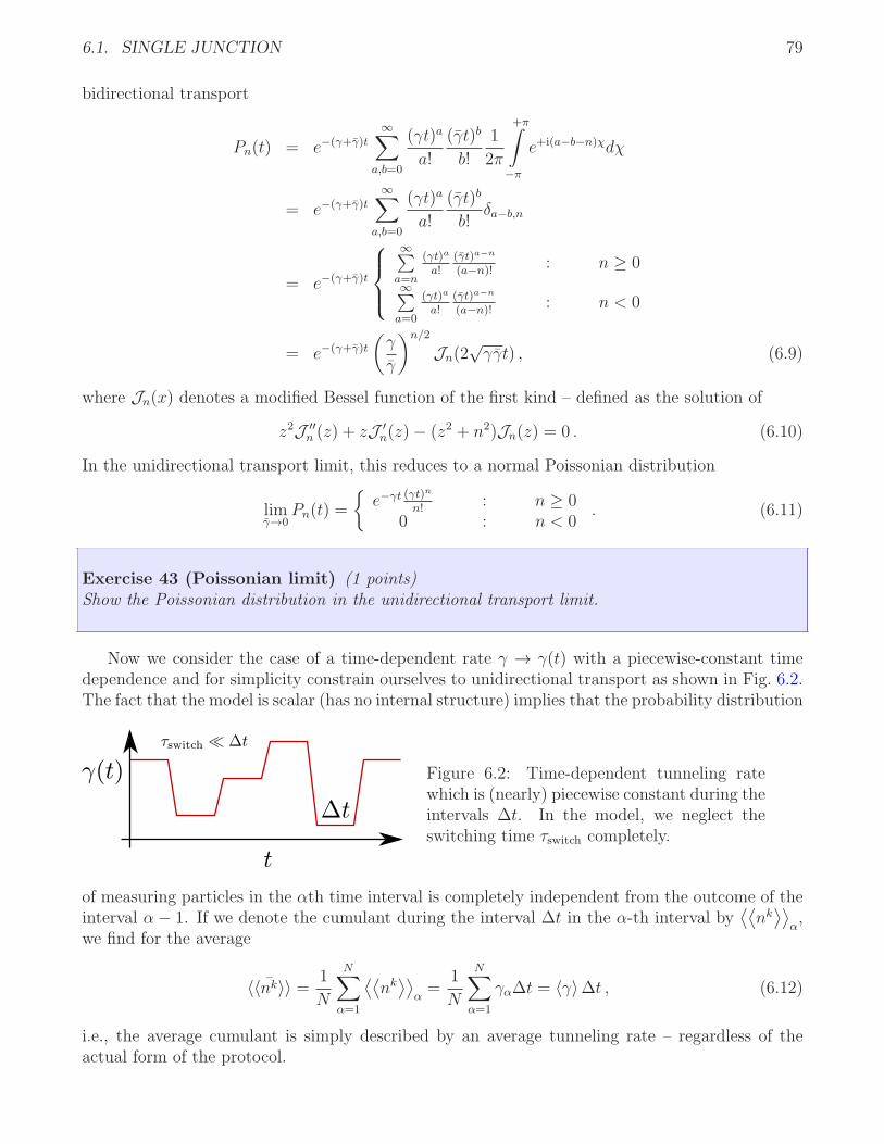
6.1. SINGLE JUNCTION 79
bidirectional transport
Pn(t) = e−(γ+γ)t
∞∑
a,b=0
(γt)a
a!
(γt)b
b!
1
2π
+π∫
−π
e+i(a−b−n)χdχ
= e−(γ+γ)t
∞∑
a,b=0
(γt)a
a!
(γt)b
b!δa−b,n
= e−(γ+γ)t
∞∑
a=n
(γt)a
a!(γt)a−n
(a−n)!: n ≥ 0
∞∑
a=0
(γt)a
a!(γt)a−n
(a−n)!: n < 0
= e−(γ+γ)t
(γ
γ
)n/2
Jn(2√γγt) , (6.9)
where Jn(x) denotes a modified Bessel function of the first kind – defined as the solution of
z2J ′′n (z) + zJ ′
n(z)− (z2 + n2)Jn(z) = 0 . (6.10)
In the unidirectional transport limit, this reduces to a normal Poissonian distribution
limγ→0
Pn(t) =
e−γt (γt)n
n!: n ≥ 0
0 : n < 0. (6.11)
Exercise 43 (Poissonian limit) (1 points)Show the Poissonian distribution in the unidirectional transport limit.
Now we consider the case of a time-dependent rate γ → γ(t) with a piecewise-constant timedependence and for simplicity constrain ourselves to unidirectional transport as shown in Fig. 6.2.The fact that the model is scalar (has no internal structure) implies that the probability distribution
Figure 6.2: Time-dependent tunneling ratewhich is (nearly) piecewise constant during theintervals ∆t. In the model, we neglect theswitching time τswitch completely.
of measuring particles in the αth time interval is completely independent from the outcome of theinterval α − 1. If we denote the cumulant during the interval ∆t in the α-th interval by
⟨⟨nk⟩⟩
α,
we find for the average
¯〈〈nk〉〉 = 1
N
N∑
α=1
⟨⟨nk⟩⟩
α=
1
N
N∑
α=1
γα∆t = 〈γ〉∆t , (6.12)
i.e., the average cumulant is simply described by an average tunneling rate – regardless of theactual form of the protocol.

80 CHAPTER 6. OPEN-LOOP CONTROL: NON-EQUILIBRIUM CASE III
6.2 Electronic pump
We consider a system with the simplest possible internal structure, which has just the two statesempty and filled. A representative of such a system is the single-electron transistor. The tunnelingof electrons through such a transistor is stochastic and thereby in some sense uncontrolled. Thisimplies that e.g. the current fluctuations through such a device (noise) can not be suppressedcompletely.
6.2.1 Time-dependent tunneling rates
We consider piecewise-constant time-dependencies of the tunneling rates ΓL(t) and ΓR(t) with anotherwise arbitrary protocol
L(χ, t) =(
−ΓL(t)fL − ΓR(t)fR +ΓL(t)(1− fL) + ΓR(t)(1− fR)e+iχ
+ΓL(t)fL + ΓR(t)fRe−iχ −ΓL(t)(1− fL)− ΓR(t)(1− fR)
)
. (6.13)
The situation is also depicted in Fig. 6.3.
Figure 6.3: Time-dependent tunneling rateswhich follow a piecewise constant protocol.Dot level and left and right Fermi functionsare assumed constant.
Let the tunneling rates during the i-th time interval be denoted by ΓiL and Γi
R and the cor-responding constant Liouvillian during this time interval by Li(χ). The density matrix after thetime interval ∆t is now given by
ρi+1 = eLi(0)∆tρi , (6.14)
such that it has no longer the form of a master equation but becomes a fixed-point iteration. Inwhat follows, we will without loss of generality assume fL ≤ fR, such that the source lead is rightand the drain lead is left. Utilizing previous results, the stationary state of the Liouvillian Li isgiven by
fi =ΓiLfL + Γi
RfRΓiL + Γi
R
(6.15)
and thereby (ΓiL/R ≥ 0) obeys fL ≤ fi ≤ fR. This implies that after a few transient iterations, the
density vector will hover around within the transport window
fL ≤ ni =⟨d†d⟩
i≤ fR ∀ i ≥ i∗ . (6.16)
The occupations will therefore follow the iteration equation(
1− ni+1
ni+1
)
= eLi(0)∆t
(1− ni
ni
)
. (6.17)

6.2. ELECTRONIC PUMP 81
To calculate the number of particles tunneling into the source reservoir, we consider the moment-generating function
Mi(χ,∆t) = Tr
eLi(χ)∆t
(1− ni
ni
)
(6.18)
and calculate the first moment
〈n〉i = (−i)∂χ Mi(χ,∆t)|χ=0
=1
(ΓiL + Γi
R)2
[
− Γ2R(fR − ni)
(
1− e−(ΓiL+Γi
R)∆t)
+ΓiLΓ
iR
(
(ni − fL)(
1− e−(ΓiL+Γi
R)∆t)
− (fR − fL)(ΓiL + Γi
R)∆t) ]
≤ 0 . (6.19)
The first term is evidently negative when ni is within the transport window fL ≤ ni ≤ fR, andthat the second term is also negative follows from its upper bound ni → fR, where we can use that1− e−x ≤ x for all x ≥ 0 which is the case for x = (Γi
L + ΓiR)∆t.
It follows that the average current always points from right (source for constant rates) to left(drain for constant rates) regardless of the actual protocol Γα
L/R chosen. In other words: With
simply modifying the tunneling rates (not taking into account whether the dot is occupied or not)it is not possible to revert the direction of the current.
6.2.2 With performing work
To obtain transport against the bias, it is therefore necessary to modify the Fermi functions e.g.by changing the chemical potentials or temperatures in the contacts. However, this first possibilitymay for fast driving destroy the thermal equilibrium in the contacts, such that we consider changingthe dot level ǫ(t). Intuitively, it is quite straightforward to arrive at a protocol that should liftelectrons from left to right and thereby pumps electrons from low to high chemical potentials, seeFig. 6.4. The propagators for the first and second half cycles read
L1(χ) =
(−Γmax
L fL(ǫmin)− Γmin
R fR(ǫmin) +Γmax
L [1− fL(ǫmin)] + Γmin
R [1− fR(ǫmin)]e+iχ
+ΓmaxL fL(ǫ
min) + ΓminR fR(ǫ
min)e−iχ −ΓmaxL [1− fL(ǫ
min)]− ΓminR [1− fR(ǫ
min)]
)
,
L2(χ) =
(−Γmin
L fL(ǫmax)− Γmax
R fR(ǫmax) +Γmin
L [1− fL(ǫmax)] + Γmax
R [1− fR(ǫmax)]e+iχ
+ΓminL fL(ǫ
max) + ΓmaxR fR(ǫ
max)e−iχ −ΓminL [1− fL(ǫ
max)]− ΓmaxR [1− fR(ǫ
max)]
)
,
(6.20)
respectively. The evolution of the density vector now follows the fixed point iteration scheme
ρ(t+ T ) = P2P1ρ(t) = eL2(0)T/2eL1(0)T/2ρ(t) . (6.21)
After a period of transient evolution, the density vector at the end of the pump cycle will approacha value where ρ(t + T ) ≈ ρ(t) = ρ. This value is the stationary density matrix in a stroboscopicsense and is defined by the eigenvalue equation
eL2(0)T/2eL1(0)T/2ρ = ρ (6.22)
with Tr ρ = 1. Once this stationary state has been determined, we can easily define the moment-generating functions for the pumping period in the (stroboscopically) stationary regime
M1(χ, T/2) = TreL1(χ)T/2ρ
, M2(χ, T/2) = Tr
eL2(χ)T/2eL1(0)T/2ρ
, (6.23)

82 CHAPTER 6. OPEN-LOOP CONTROL: NON-EQUILIBRIUM CASE III
Figure 6.4: Here, tunneling rates and the dotlevel also follow a piecewise constant protocol,which admits only two possible values (top leftand right) and is periodic (see left panel). Thestate of the contacts is assumed as stationary.For small pumping cycle times T , the protocolis expected to pump electrons from the left to-wards the right contact and thereby lifts elec-trons to a higher chemical potential.
where M1 describes the statistics in the first half cycle and M2 in the second half cycle and themoments can be extracted in the usual way. The distribution for the total number of particlestunneling during the complete pumping cycle n = n1 + n2 is given by
Pn(T ) =∑
n1,n2 : n1+n2=n
Pn1(T/2)Pn2(T/2) =∑
n1,n2
δn,n1+n2Pn1(T/2)Pn2(T/2) . (6.24)
Then, the first moment may be calculated by simply adding the first moments of the particlestunneling through both half-cycles
〈n〉 =∑
n
nPn =∑
n
n∑
n1,n2
δn,n1+n2Pn1(T/2)Pn2(T/2) =∑
n1,n2
(n1 + n2)Pn1(T/2)Pn2(T/2)
= 〈n1〉+ 〈n2〉 . (6.25)
In the following, we will constrain ourselves for simplicity to symmetric tunneling rates ΓminL =
ΓminR = Γmin and Γmax
L = ΓmaxR = Γmax. In this case, we obtain the simple expression for the average
number of particles during one pumping cycle
〈n〉 =ΓmaxΓmin
Γmax + Γmin
T
2
[fL(ǫ
max)− fR(ǫmax) + fL(ǫ
min)− fR(ǫmin)
]
+Γmax − Γmin
(Γmax + Γmin)2[Γmax
(fL(ǫ
min)− fR(ǫmax)
)+ Γmin
(fR(ǫ
min)− fL(ǫmax)
)]×
× tanh
[T
4
(Γmin + Γmax
)]
. (6.26)
The first term (which dominates for slow pumping, i.e., large T ) is negative when fL(ω) < fR(ω).It is simply given by the average of the two SET currents one would obtain for the two half cycles.

6.2. ELECTRONIC PUMP 83
The second term however is present when Γmax > Γmin and may be positive when the dot levelis changed strongly enough souch that fL(ǫ
min) > fR(ǫmax) and fR(ǫ
min) > fL(ǫmax). For large
differences in the tunneling rates and small pumping times T it may even dominate the first term,such that the net particle number may be positive even though the bias would favor the oppositecurrent direction, see Fig. 6.5. The second cumulant can be similarly calculated
⟨n2⟩− 〈n〉2 =
⟨n21
⟩− 〈n1〉2 +
⟨n22
⟩− 〈n2〉2 . (6.27)
Exercise 44 (Second Cumulant for joint distributions) (1 points)Show the validity of the above equation.
50 100 150 200
pump cycle time T-1
-0,5
0
0,5
1
1,5
2
part
icle
num
ber
<n(
T)>
/ Fa
no f
acto
r F
<n> (error sqrt[<n2>-<n>
2])
Fano factor FT = [<n
2>-<n>
2]/|<n>|
Figure 6.5: Average number of tunneled particles during one pump cycle. Parameters have beenchosen as Γmax = 1, Γmin = 0.1, fL(ǫ
min) = 0.9, fR(ǫmin) = 0.95, fL(ǫ
max) = 0, fR(ǫmax) = 0.05,
such that for slow pumping (large T ), the current I = 〈n〉 /T must become negative. The shadedregion characterizes the width of the distribution, and the Fano factor demonstrates that aroundthe maximum pump current, the signal-to-noise ratio is most favorable.
When the dot level is shifted to very low and very large values (large pumping power), the biasis negligible (alternatively, we may also consider an unbiased situation from the beginning). Inthis case, we can assume fL(ǫ
min) = fR(ǫmin) = f(ǫmin) and fL(ǫ
max) = fR(ǫmax) = f(ǫmax). Then,
the second term dominates always and the particle number simplifies to
〈n〉 =[f(ǫmin)− f(ǫmax)
] Γmax − Γmin
Γmax + Γmintanh
[T
4
(Γmin + Γmax
)]
. (6.28)

84 CHAPTER 6. OPEN-LOOP CONTROL: NON-EQUILIBRIUM CASE III
This becomes maximal for large pumping time and large power consumption (f(ǫmin)− f(ǫmax) =1). In this idealized limit, we easily obtain for the Fano factor for large cycle times T
FT =〈n2〉 − 〈n〉2
|〈n〉|T→∞→ 2ΓmaxΓmin
(Γmax + Γmin)2, (6.29)
which demonstrates that the pump works efficient and noiseless when Γmax ≫ Γmin.At infinite bias fL(ω) = and fR(ω) = 0, the pump does not transport electrons against any
potential or thermal gradient but can still be used to control the statistics of the tunneled electrons.For example, it is possible to reduce the noise to zero also in this limit when Γmin → 0.
Chapter 7
Closed-loop control:Non-Equilibrium Case IV
Closed-loop (or feedback) control means that the system is monitored (either continuously or atcertain times) and that the result of these measurements is fed back by changing some parameter ofthe system. Under measurement with outcome m (an index characterizing the possible outcomes),the density matrix transforms as
ρm→ MmρM
†m
Tr
M †mMmρ
, (7.1)
and the probability at which this outcome occurs is given by TrM †
mMm
. This can also be
written in superoperator notation
ρm→ Pmρ
Tr Pmρ. (7.2)
Let us assume that conditioned on the measurement result m at time t, we apply a propagatorfor the time interval ∆t. Then, a measurement result m at time t provided, the density matrix attime t+∆t will be given by
ρ(m)(t+∆t) = eL(m)∆t Pmρ
Tr Pmρ. (7.3)
However, to obtain an effective description of the density matrix evolution, we have to averageover all measurement outcomes – where we have to weight each outcome by the correspondingprobability
ρ(t+∆t) =∑
m
Tr Pmρ(t) eL(m)∆t Pmρ
Tr Pmρ=∑
m
eL(m)∆tPmρ(t) . (7.4)
Note that this is an iteration scheme, the conditioned Liouvillian L(m) may well depend on the timet (at which the measurement is performed) as long as it is constant during the interval [t, t+∆t].
7.1 Single junction
To start with the simplest possible system, we reconsider here the case of a single junction in theunidirectional transport limit, which is described by
ρn = γρn−1 − γρn , (7.5)
85

86 CHAPTER 7. CLOSED-LOOP CONTROL: NON-EQUILIBRIUM CASE IV
where the parameter γ describes the speed at which the resulting Poissonian distribution
ρn(∆t) =
e−γ∆t (γ∆t)n
n!: n ≥ 0
0 : n < 0(7.6)
moves towards larger n. When we arrange the probabilities in an infinite-dimensional vector, themaster equation becomes
d
dt
...ρn−1
ρn...
=
. . .
. . . −γ+γ −γ
. . . . . .
...ρn−1
ρn...
. (7.7)
For the initial state ρn(0) = δn,0 we have written the solution explicitly. Using the translationalinvariance in n and the superposition principle, we can therefore write the general solution explicitlyas
ρ0(t+∆t)ρ1(t+∆t)ρ2(t+∆t)
...ρn(t+∆t)
...
= e−γ∆t
1γ∆t 1(γ∆t)2
2γ∆t 1
......
. . . . . .(γ∆t)n
n!(γ∆t)n−1
(n−1)!. . . . . .
......
ρ0(t)ρ1(t)ρ2(t)...
ρn(t)...
(7.8)
which takes the form ρ(t + ∆t) = W(∆t)ρ(t) with the infinite-dimensional propagation matrixW(∆t).
Exercise 45 (Probability conservation) (1 points)Show that the above introduced propagator W(∆t)preserves the sum of all probabilities, i.e., that∑
n ρn(t+∆t) =∑
n ρn(t).
We have found previously that an open-loop control scheme does not drastically modify thepicture. We do now consider regular measurements of the number of tunneled particles beingperformed at time intervals ∆t. The major difference to our previous considerations is now thatwe modify the tunneling rate γ in dependence on the initial state ρ(t) and on the time t, i.e., wehave γ → γm(t), where m denotes the total number of particles measured at time t. Then, thepropagation matrix becomes (omitting for brevity the dependence on t in the rates)
W(t,∆t) =
e−γ0∆t
e−γ0∆t(γ0∆t) e−γ1∆t
e−γ0∆t (γ0∆t)2
2e−γ1∆t(γ1∆t) e−γ2∆t
......
.... . .
e−γ0∆t (γ0∆t)n
n!e−γ1∆t (γ1∆t)n−1
(n−1)!e−γ2∆t (γ2∆t)n−2
(n−2)!. . .
......
.... . .
. (7.9)

7.1. SINGLE JUNCTION 87
When we would denote the normal propagator in Eq. (7.8) with an index i as W (i) = W|γ=γi, the
full effective feedback propagator can also be written as
W(t,∆t) =∑
n
W (n)(t,∆t)P (n) , (7.10)
where the matrix elements of the projection superoperator P (n)ij = δinδjn vanish except at position
n on the diagonal.
Exercise 46 (Effective Feedback Propagator) (1 points)Show the validity of Eq. (7.10).
This naturally includes the measurement process into the description of feedback: Measuringn tunneled particles at time t projects the density vector as
ρ(t) → P (n)ρ(t)
Tr P (n)ρ(t) , (7.11)
which occurs with probability TrP (n)ρ(t)
. When we compute the average outcome of such
a measurement but do not perform any feedback, we have to multiply with the correspondingprobability to obtain the average density matrix at time t+∆t
ρ(t+∆t) =∑
n
W(t,∆t)P (n)ρ(t) = W(t,∆t)ρ(t) . (7.12)
With feedback however, a propagator that is conditioned on the measurement result has to beapplied
ρ(t+∆t) =∑
n
W (n)(t,∆t)P (n)ρ(t) , (7.13)
which corresponds to Eq. (7.10).The matrix elements of the effective feedback propagatoor read
Wnm(t,∆t) =
e−γm∆t (γm∆t)(n−m)
(n−m)!: n ≥ m
0 : n < m, (7.14)
where e.g. one simple feedback protocol would be given by
γm(t) =
γ + α
(γ − m
t
): m ≤ γt
[1 + 1
α
]
0 : else. (7.15)
Such a feedback protocol would aim to stabilize a mean of m = γt and should also keep the widthof the distribution at a finite value. For general feedback protocols, we obtain for the first momentat time t+∆t
〈n〉t+∆t =∑
n
nρn(t+∆t) =∑
n
n∑
m
Wnm(t,∆t)ρm(t) =∑
m
[∑
n
nWnm(t,∆t)
]
ρm(t)
=∑
m
[ ∞∑
n=m
ne−γm∆t (γm∆t)(n−m)
(n−m)!
]
ρm(t) =∑
m
[ ∞∑
n=0
(n+m)e−γm∆t (γm∆t)n
n!
]
ρm(t)
=∑
m
(γm∆t+m) ρm(t) = 〈γn〉t ∆t+ 〈n〉t , (7.16)

88 CHAPTER 7. CLOSED-LOOP CONTROL: NON-EQUILIBRIUM CASE IV
such that the change of the first moment during time interval ∆t is determined by the averagetunneling rate. Similarly, we obtain for the second moment
⟨n2⟩
t+∆t=
∑
n
n2ρn(t+∆t) =∑
m
[ ∞∑
n=0
(n+m)2e−γm∆t (γm∆t)n
n!
]
ρm(t)
=∑
m
[γm∆t (1 + γm∆t) + 2γm∆tm+m2
]ρm(t)
=⟨γ2n
⟩
t∆t2 + 〈γn(1 + 2n)〉t ∆t+
⟨n2⟩
t. (7.17)
This implies for the variance under feedback⟨n2⟩
t+∆t− 〈n〉2t+∆t = ∆t2
[⟨γ2n
⟩
t− 〈γn〉2t
]+∆t [〈γn〉t + 2 〈γnn〉t − 2 〈γn〉t 〈n〉t]
+⟨n2⟩
t− 〈n〉2t . (7.18)
For large ∆t, the first term on the r.h.s. will dominate, such that due to 〈γ2n〉t − 〈γn〉2t =
⟨(γn − 〈γn〉)2
⟩≥ 0 the variance will always increase. For small ∆t however, the second term
may dominate, such that for adapted feedback protocols, the variance of the distribution maydecrease during ∆t.
Exercise 47 (Variance evolution without feedback) (1 points)Show that without feedback γm(t) = γ, the variance during the iteration will for arbitrary distribu-tions always increase as
(〈n2〉t+∆t − 〈n〉2t+∆t
)−(〈n2〉t − 〈n〉2t
)= γ∆t.
It is however clear that the resulting distribution cannot have a completely vanishing width,as for this case one would also obtain a growing variance in time.
Exercise 48 (Variance evolution of a localized distribution) (1 points)Show that for arbitrary feedback, the variance of a localized distribution ρm(t) = δmm the variancewill always increase unless γm = 0.
Therefore, the resulting time-dependent distribution may be expected to have a finite width ifthe iteration scheme is performed in a range where the feedback is negative. This can be illustratedat the example of a continuous (n → x) Gaussian distribution
ρx(t) =1√2πσ
e−(x−γt)2
2σ2 (7.19)
with mean µ = γt = 〈x〉t and width σ. The control scheme
γx(t) = γeαe−αxγt (7.20)
leads to the following expectation values (replacing sums by integrals and extending the integrationrange over the complete real axis)
〈γx〉 = γeα2σ2
2γ2t2 ,⟨γ2x
⟩= γ2e
2α2σ2
γ2t2 , 〈xγx〉 = eα2σ2
2γ2t2
[
γ2t− ασ2
t
]
, (7.21)

7.1. SINGLE JUNCTION 89
which leads to a change of the variance of
∆σ2 = ∆t2[⟨γ2x
⟩
t− 〈γx〉2t
]+∆t [〈γx〉t + 2 〈xγx〉t − 2 〈x〉t 〈γx〉t]
= ∆t2γ2eα2σ2
γ2t2
[
eα2σ2
γ2t2 − 1
]
+∆t
te
α2σ2
2γ2t2[γt− 2ασ2
]. (7.22)
Neglecting the quadratic contribution (small ∆t) the variance is stabilized when the feedbackstrength is adapted with time and width of the distribution α ≥ γt
2σ2 . This is also confirmedby the numerical propagation of an initially localized probability distribution with the iterationscheme (7.12) in Fig. 7.1. Without feedback (thin lines), the distribution propagates, but also
0 20 40 60 80 100 120
particle number n
0
0,2
0,4
0,6
0,8
1
feed
back
dis
trib
utio
n P
n(t)
t=100t=80t=60t=40t=20t=0
-50 -25 0 25 50n - γ t
10-6
10-5
10-4
10-3
10-2
10-1
t=100t=200t=300t=400t=500Gauss fit: σ=7.1
sampling N=104
Figure 7.1: Plot of probability distributions Pn(t) without feedback (Poissonian evolution, thinlines), with constant feedback strength (medium thickness) and with time-proportional feedbackstrength (thick curves). The inset shows the long-time evolution for constant feedback strength(increasing width) and time-proportional feedback strength (stationary width). The fit (dashedcurve) demonstrates that the stationary distribution is Gaussian. In addition, a direct sampling ofthe feedback protocol yields the same distribution. Parameters: γ = 1, ∆t = 1, α = 1 for constantfeedback and α = 0.01t for time-proportional feedback.
increases its width in time. With constant feedback strength, the distribution propagates at thesame speed and its width is reduced but still increases with time for sufficiently large times. Onlywhen the feedback strength is chosen to scale linarly in time, the shape of the distribution becomesstabilized. This in turn allows to determine the stationary width in dependence of the feedbackstrength α = α0t as follows: Inserting this dependence in Eq. (7.22) leads to a condition under
90 CHAPTER 7. CLOSED-LOOP CONTROL: NON-EQUILIBRIUM CASE IV
which the variance of a Gaussian distribution remains constant
0 = (γ∆t)ey/2 [ey − 1] + 1− 2γ
α0
y (7.23)
with the variable
y =α20σ
2
γ2. (7.24)
This transcendental equation can for given ∆t, γ and α0 be solved numerically for y, which in turnenables one to determine the stationary width σ. For example, for γ∆t = 1 and γ/α0 = 100 wefind a numerical solution y ≈ 0.005025, which corresponds to a width of σ ≈ 7.1. This width isexactly found in the Gaussian fit of the numerical solution (compare the inset of Fig. 7.1). Thevalidity of this effective description under feedback is further underlined by a direct sampling ofthe feedback protocol (also compare the inset): Here, the feedback parameter is adjusted at finitetime intervals ∆t, and dependent on the previous measurement result. Therefore, under the chosenfeedback protocol
γn(t) = γeα0te−α0nγ (7.25)
the long-term limit leads to a frozen distribution which propagates with a constant shape.
These findings can be made more explicit for linear feedback of the form
γn(t) = γ [1− g(n− γt)] (7.26)
with the dimensionless feedback parameter g > 0. It can be thought of an approximation of scheme(7.25) for small g = α0/γ ≪ 1. Of course, the above scheme formally allows for negative rateswhen n ≫ γ0t. In reality however, the probability for such a process is exponentially suppressedfor sufficiently large times, since for large times the width of a Poissonian process is sufficientlysmaller than its mean value σ/µ = 1/
√γt. The linear feedback scheme has the advantage that
Eqns. (7.16) and (7.18) only couple to themselves and can thus be solved
C1(t+∆t)− C1(t) = γ∆t [1− gC1(t) + gγt] ,
C2(t+∆t)− C2(t) = γ2∆t2g2C2(t) + γ∆t [1 + γgt− gC1(t)− 2gC2(t)] . (7.27)
In the limit of small ∆t, the differential version of these equations read
C1 = γ [1− gC1(t) + gγt] ,
C2 = γ [1 + γgt− gC1(t)− 2gC2(t)] (7.28)
and admit for the initial conditions C1(0) = 0 and C2(0) = 0 the simple solution
C1(t) = γt , C2(t) =1− e−2gγt
2g, (7.29)
which shows a continuous evolution towards a constant width of σ =√
limt→∞
C2(t) =1√2g.

7.2. MAXWELL’S DEMON 91
7.2 Maxwell’s demon
Maxwell invented his famous demon as a thought experiment to demonstrate that thermodynamicsis a macroscopic effective theory: An intelligent being (the demon) living in a box is measuringthe speed of molecules of some gas in the box. An initial thermal distribution of molecules impliesthat the molecules have different velocities. The demon measures the velocities and inserts animpermeable wall whenever the the molecule is too fast or lets it pass into another part of the boxwhen it is slow. As time progresses, this would lead to a sorting of hot and cold molecules, andthe temperature difference could be exploited to perform work.
This is nothing but a feedback (closed-loop) control scheme: The demon performs a mea-surement (is the molecule slow or fast) and then uses the information to perform an appropriatecontrol action on the system (inserting a wall or not). Classically, the insertion of a wall requiresin the idealized case no work, such that only information is used to create a temperature gradient.However, the Landauer principle states that with each bit of information erased, heat of at leastkBT ln(2) is dissipated into the environment. To remain functionable, the demon must at somepoint start to delete the information, which leads to the dissipation of heat. The dissipated heatwill exceed the energy obtainable from the thermal gradient.
An analog of a Maxwell demon may be implemented in an electronic context: There, anexperimentalist takes the role of the demon. The box is replaced by the SET (including thecontacts), on which by a nearby QPC a measurement of the dot state (simply empty or filled) isperformed. Depending on the measurement outcome, the tunneling rates are modified in time ina piecewise constant manner: When there is no electron on the dot, the left tunneling rate ΓL isincreased (low barrier) and the right tunneling rate ΓR is decreased (high barrier). The oppositeis done when there is an electron on the dot, see Fig. 7.2. Thus, the only difference in comparison
0 200 400 600 800 1000
0,1
0,2
0,3
mea
sure
d Q
PC
cu
rren
t SET
SET
Figure 7.2: Sketch of the feedback scheme: For a filled dot (low QPC current), the left tunnelingrate is minimal and the right tunneling rate is maximal and vice-versa for an empty dot. The dotlevel itself is not changed.
to Sec. 6.2.1 is that now information of the system is used to modify the tunneling rates. Verysimple considerations already demonstrate that with this scheme, it will be possible to transportelectrons against an existing bias only with time-dependent tunneling rates. When one junction is

92 CHAPTER 7. CLOSED-LOOP CONTROL: NON-EQUILIBRIUM CASE IV
completely decoupled ΓminL/R → 0, this will completely rectify the transport from left to right also
against the bias (if the bias is finite). In the following, we will address the statistics of this device.The first step is to identify an effective evolution equation for the density matrix accounting
for measurement and control. In this case, both processes occur continuously, which enables us to
consider infinitesimally small time intervals ∆t. For an empty dot at time t, i.e., for ρE(t) =
(10
)
,
the density vector at time t+∆t will be given by
ρE(t+∆t) =[1+∆tL(E)
]ρE(t) . (7.30)
Similarly, we have for a filled dot ρE(t) =
(01
)
ρF (t+∆t) =[1+∆tL(F )
]ρF (t) . (7.31)
Both equations can be combined using a projection superoperator
ρ(t+∆t) =[1+∆tL(E)
]PE +
[1+∆tL(F )
]PF
ρ(t) (7.32)
with the operators
PE =
(1 00 0
)
, PF =
(0 00 1
)
. (7.33)
Since we have PE + PF = 1, this defines when ∆t → 0 (continous control limit) an effectiveLiouvillian
Leff = L(E)PE + L(F )PF , (7.34)
which is in complete equivalence with Eq. (7.10) when ∆t → 0. Note that this can be performedwith and without counting fields. Taking into account the diagonal structure of the projectionsuperoperators, this simply implies that the effective Liouvillian under feedback has the first columnfrom the Liouvillian conditioned on an empty dot and the second column from the Liouvillianconditioned on the filled dot
Leff(χL, χR) =
(−ΓE
LfL − ΓERfR +ΓF
L(1− fL)e+iχL + ΓF
R(1− fR)e+iχR
+ΓELfLe
−iχL + ΓERfRe
−iχR −ΓFL(1− fL)− ΓF
R(1− fR)
)
. (7.35)
Evidently, it still obeys trace conservation but now the tunneling rates in the two columns aredifferent ones.
Exercise 49 (Current at zero bias) (1 points)Calculate the feedback-current at zero bias fL = fR = f in dependence on f . What happens at zerotemperatures, where f → 0, 1?
The effective Liouvillian describes the average evolution of trajectories under continuous mon-itoring and feedback. The validity of the effective description can be easily checked by calculatingMonte-Carlo solutions as follows:

7.2. MAXWELL’S DEMON 93
Starting e.g. with a filled dot, the probability to jump out e.g. to the right lead during thesmall time interval ∆t reads P
(F )out,R = ΓF
R(1−fR)∆t. Similarly, we can write down the probabilitiesto jump out to the left lead and also the probabilities to jump onto an empty dot from either theleft or right contact
P(F )out,R = ΓF
R(1− fR)∆t , P(F )out,L = ΓF
L(1− fL)∆t ,
P(E)in,R = ΓE
RfR∆t , P(E)in,L = ΓE
LfL∆t . (7.36)
Naturally, these jump probabilities also uniquely determine the change of the particle number oneither contact. The remaining probability is simply the one that no jump occurs during ∆t. AMonte-Carlo simulation is obtained by drawing a random number and choosing one out of threepossible outcomes for empty (jumping in from left contact, from right contact, or remaining empty)and for a filled (jumping out to left contact, to right contact, or remaining filled) dot. Repeatingthe procedure several times yields a single trajectory for n(t), nL(t), and nR(t). The ensembleaverage of many such trajectories agree perfectly with the solution
〈n〉t = Trd†deLeff(0,0)tρ0
,
〈nL〉t = (−i∂χ) TreLeff(χ,0)tρ0
∣∣χ=0
,
〈nR〉t = (−i∂χ) TreLeff(0,χ)tρ0
∣∣χ=0
(7.37)
of the effective feedback master equation, see Fig. 7.3. To compare with the case without feedback,we parametrize the change of tunneling rates by dimensionless constants
ΓEL = eδ
ELΓL , ΓE
R = eδERΓR , ΓF
L = eδFLΓL , ΓF
R = eδFRΓR , (7.38)
where δβα → 0 reproduces the case without feedback and δβα > 0(< 0) increases (decreases) thetunneling rate to contact α conditioned on dot state β. The general current can directly becalculated as
I =fL(1− fR)Γ
ELΓ
FR − (1− fL)fRΓ
FLΓ
ER
ΓELfL + ΓF
L(1− fL) + ΓERfR + ΓF
R(1− fR), (7.39)
which reduces to the conventional current without feedback when Γβα → Γα. For finite feedback
strength however, this will generally induce a non-vanishing current at zero bias, see Fig. 7.4.In our idealized setup, this current is only generated by the information on whether the dot isoccupied or empty – hence the interpretation as a Maxwell demon. When the contacts are held atequal temperatures βL = βR = β, this raises the question for the maximum power
P = −IV (7.40)
generated by the device.In what follows, we will consider symmetric feedback characterized by a single parameter
∆EL = ∆F
R = −∆FL = −∆E
R = +δ , (7.41)
where δ > 0 favors transport from left to right and δ < 0 transport from right to left and alsosymmetric tunneling rates Γ = ΓL = ΓR. With these assumptions, it is easy to see that for largefeedback strengths δ ≫ 1, the current simply becomes
I → ΓeδfL(1− fR)
fL + (1− fR). (7.42)

94 CHAPTER 7. CLOSED-LOOP CONTROL: NON-EQUILIBRIUM CASE IV
0
0,2
0,4
0,6
0,8
1
n SET(t
)
-0,5
0
0,5n L
(t)/
t
5 10 15
dimensionless time Γ t
-0,5
0
0,5
n R(t
)/t
no feedback referenceN
traj=1
Ntraj
=100
Ntraj
=10000
feedback ME
Figure 7.3: Comparison of a single (thin red curve with jumps, same realization in all panels) andthe average of 100 (medium thickness, green) and 10000 (bold smooth curve, turquoise) trajectorieswith the solution from the effective feedback master equation (thin black) for the dot occupation(top), the number of particles on the left (middle), and the number of particles on the right(bottom). The average of the trajectories converges to the effective feedback master equationresult. The reference curve without feedback (dashed orange) may be obtained by using vanishingfeedback parameters and demonstrates that the direction of the current may actually be reversedvia sufficiently strong feedback. Parameters: ΓL = ΓR ≡ Γ, fL = 0.45, fR = 0.55, δEL = δFR = 1.0,δER = δFL = −10.0, and Γ∆t = 0.01.
To determine the maximum power, we would have to maximize with respect to left and rightchemical potentials µL and µR, the lead temperature β and the dot level ǫ. However, as theseparameters only enter implicitly in the Fermi functions, it is more favorable to use that for equaltemperatures
β(µL − µR) = βV = ln
[fL(1− fR)
(1− fL)fR
]
, (7.43)
such that we can equally maximize
P = −IV =1
β(−IβV ) → Γeδ
β
[
− fL(1− fR)
fL + (1− fR)ln
(fL(1− fR)
(1− fL)fR
)]
. (7.44)
The term in square brackets can now be maximized numerically with respect to the parametersfL and fR in the range 0 ≤ fL/R ≤ 1, such that one obtains for the maximum power at strongfeedback
P ≤ kBTΓeδ0.2785 at fL = 0.2178 fR = 0.7822 . (7.45)
The average work performed between two QPC measurement points at t and t + ∆t is thereforegiven by
W ≤ kBTΓeδ∆t0.2785 . (7.46)

7.2. MAXWELL’S DEMON 95
-4 -3 -2 -1 0 1 2 3 4
dimensionless bias voltage β V
curr
ent I
[Γ]
no feedbackpiecewise constant feedback
Figure 7.4: Current voltage characteristicsfor finite feedback strength δ = 1 (red curve)and without feedback δ = 0 (black curve).For finite feedback, the current may pointin the other direction than the voltage lead-ing to a positive power P = −IV (shadedregion) generated by the device.
However, to perform feedback efficiently, it is required that the QPC sampling rate is fast enoughthat all state changes of the SET are faithfully detected (no tunneling charges are missed). Thisrequires that Γeδ∆t < 1. Therefore, we can refine the upper bound for the average work
W ≤ kBT0.2785 . (7.47)
This has to be contrasted with the Landauer principle, which states that for each deleted bit inthe demons brain (each QPC data point enconding high current or low current) heat of
Q ≥ kBT ln(2) ≈ kBT0.6931 (7.48)
is dissipated. The second law is therefore not violated.
The conventional fluctuation theorem for the SET at equal temperatures
P+n(t)
P−n(t)= enβV (7.49)
is modified in presence of feedback. However, since the Liouvillian still contains the countingfields in the conventional way, simply the factor in the exponential, not the dependence on thenumber of tunneled electrons n is changed. To evaluate the FT, we identify symmetries in themoment-generating function (or alternatively the eigenvalues of the Liouvillian)
λ(−χ) = λ
(
+χ+ i ln
[
e+4δ fL(1− fR)
(1− fL)fR
])
= λ(+χ+ i ln
[e+4δeβV
])
= λ(+χ+ i(4δ + βV )) . (7.50)
From this symmetry of the cumulant-generating function we obtain for the fluctuation theoremunder feedback
limt→∞
P+n(t)
P−n(t)= en(βV+4δ) = enβ(V−V ∗) , (7.51)
where V ∗ = −4δ/β denotes the voltage at which the current (under feedback) vanishes.

96 CHAPTER 7. CLOSED-LOOP CONTROL: NON-EQUILIBRIUM CASE IV
Exercise 50 (Vanishing feedback current) (1 points)Show for equal temperatures that the feedback current vanishes when V = V ∗ = −4δ/β.
However, piecewise constant feedback is not the only relevant scheme. As a further example,let us consider instantaneously applying a fast and short pulse on the tunneling rates wheneverthe QPC detects a change in the dots occupation, see Fig. 7.5. To change the counting statistics,
0 200 400 600 800 1000
0,1
0,2
0,3
me
asu
red
QP
C c
urr
en
t
SET SET
Figure 7.5: Sketch of the modified feedbackscheme: This time, feedback control oper-ations are not conditioned on the state ofthe dot, but on its change. Whenever anelectron has jumped into the dot (red ar-rows), the left tunneling rate is decreasedand the right tunneling rate is increases withan instantaneous pulse. The opposite is donewhen an electron has jumped out of the dot(green arrows). The dot level itself is notchanged. To obtain a significant change ofthe statistics, it is necessary that particlesmay also tunnel during the pulses. Thisopens the possibility of setting up feedbackschemes with a finite recursion depth: Elec-trons tunneling during the control opera-tions may trigger further control operationsand so on – eventually limited by the finiteprocessing speed of the apparatus and otherfactors.
the infinitely short pulse of this feedback scheme must be infinitely large and can thus be wellrepresented by a δ function. Since for an SET the QPC does not resolve the direction of theelectronic jumps, we can only perform control operations conditioned on particles jumping in andout
L(t) = L0 +∑
tin
L(I) +∑
tout
L(O) , (7.52)
where tin and tout denote the times at which an electron jumps in or out of the dot, respectively.The control Liouvillians have the form
L(I) = δ(t− tin)
(−δILfL − δIRfR +δIL(1− fL)e
+iχL + δIR(1− fR)e+iχR
+δILfLe−iχL + δIRfRe
−iχR −δIL(1− fL)− δIR(1− fR)
)
,
L(O) = δ(t− tout)
(−δOL fL − δORfR +δOL (1− fL)e
+iχL + δOR(1− fR)e+iχR
+δOL fLe−iχL + δORfRe
−iχR −δOL (1− fL)− δOR(1− fR)
)
,(7.53)
where δβα > 0 denote dimensionless feedback parameters and δβα = 0 reproduces the case without

7.2. MAXWELL’S DEMON 97
feedback. This implies a simple form of the corresponding (dimensionless) propagators
eκI
= exp
(−δILfL − δIRfR +δIL(1− fL)e
+iχL + δIR(1− fR)e+iχR
+δILfLe−iχL + δIRfRe
−iχR −δIL(1− fL)− δIR(1− fR)
)
,
eκO
= exp
(−δOL fL − δORfR +δOL (1− fL)e
+iχL + δOR(1− fR)e+iχR
+δOL fLe−iχL + δORfRe
−iχR −δOL (1− fL)− δOR(1− fR)
)
(7.54)
during such an infinitesimally short pulse.
Exercise 51 (δ-kick propagator) (1 points)Calculate the general propagator for a time-dependent Liouvillian of the piecewise-constant form
L = L0 + LcΘ(t− tc)Θ(tc + τc − t) ,
where tc denotes the control time and τc the control duration. What is the propagator when Lc =κ/τc in the limit τc → 0?
With these Liouvillians it is still necessary to derive an effective Liouvillian under feedback.For tunneling events during the baseline propagation, we have for the conditional density matrixat time t+∆t
ρ(nL,nR)(t+∆t) =
(1
2π
)2+π∫
−π
exp [L0(χL, χR)∆t− inLχL − inRχR] dχLdχRρ(t) , (7.55)
where nL and nR denote the number of particles that have tunneled to the left and right junctionduring ∆t, respectively. Since we are interested in continous monitoring, it suffices to expand tofirst order in ∆t. With the splitting of the Liouvillian
L0(χL, χR) = L(0,0) + L(1,0)e+iχL + L(−1,0)e−iχL + L(0,1)e+iχR + L(0,−1)e−iχR (7.56)
it becomes obvious that for small ∆t only single-tunneling events need to be considered. Thesuperoperators
J 00(∆t) =
(1
2π
)2+π∫
−π
exp [L0(χL, χR)∆t] dχLdχR ≈ 1+ L(0,0)∆t ,
J ±1,0(∆t) =
(1
2π
)2+π∫
−π
exp [L0(χL, χR)∆t∓ iχL] dχLdχR ≈ L±1,0∆t ,
J 0,±1(∆t) =
(1
2π
)2+π∫
−π
exp [L0(χL, χR)∆t∓ iχR] dχLdχR ≈ L0,±1∆t (7.57)
now take the role of projection superoperators for a measurement of the particle numbers nL andnR during ∆t. The effective propagator under feedback from t to t+∆t can be written as
ρ(t+∆t) =∑
α
Wα(∆t)Pαρ(t) , (7.58)

98 CHAPTER 7. CLOSED-LOOP CONTROL: NON-EQUILIBRIUM CASE IV
where Wα(∆t) denotes the propagator conditioned on measurement result α and Pα the corre-sponding projection superoperator. In the continous measurement limit, this defines an effectiveLiouvillian via solving
ρ(t+∆t) =[
1+∆tL0,0 + eκO
∆t(L(0,1) + L(1,0)
)+ eκ
I
∆t(L(0,−1) + L(−1,0)
)]
ρ(t) (7.59)
for the difference quotient (ρ(t+∆t)−∆t)/∆t and letting ∆t → 0. With counting fields, it reads
Leff = L(0,0) + eκO(χL,χR)
(e+iχRL(0,1) + e+iχLL(1,0)
)+ eκ
I(χL,χR)(e−iχRL(0,−1) + e−iχLL(−1,0)
),(7.60)
where it becomes quite obvious that the dependence on the counting fields becomes nontrivial.This is valid for a recursion depth zero, i.e., particles tunneling during the control operations donot trigger further control operations. As with the piecewise constant scheme, this may also becompared to a Monte-Carlo simulation of the feedback scheme, see Fig. 7.6 . For some analytic
0
0,2
0,4
0,6
0,8
1
n SET(t
)
-0,5
0
0,5
n L(t
)/t
5 10 15
dimensionless time Γ t
-0,5
0
0,5
n R(t
)/t
no-feedback referenceN
traj=1
Ntraj
=100
Ntraj
=10000
feedback ME
Figure 7.6: The average of the Monte-Carlotrajectories converges to the effective feed-back master equation result. Control op-erations (bold kinks in top graph) are notalways correlated with a change in the occu-pation or the particle number left and right,since only the net particle number after con-trol is displayed. Parameters: ΓL = ΓR ≡ Γ,fL = 0.45, fR = 0.55, δIL = δOR = 0,δIR = δOL = 1.0, and Γ∆t = 0.01.
understanding, let us assume that the control pulses only affect a single junction at a time with asimilar feedback strength
eκI(χR) = exp
(−δfR +δ(1− fR)e
+iχR
+δfRe−iχR −δ(1− fR)
)
δ→∞→(
1− fR e+iχR(1− fR)e−iχRfR fR
)
,
eκO(χL) = exp
(−δfL +δ(1− fL)e
+iχL
+δfLe−iχL −δ(1− fL)
)
δ→∞→(
1− fL e+iχL(1− fL)e−iχLfL fL
)
, (7.61)
where the propagators have a finite limit even in the limit of infinite feedback strength.
Exercise 52 (Infinite Feedback Strength) (1 points)Show that for infinite feedback strength coupling to a single junction leads to an immediate equili-bration of the density matrix with the contact to which it is coupled during control.
Therefore, the effective Liouvillian for infinite feedback strength is given by
Leff(χL, χR) =
(−ΓLfL − ΓRfR 0
0 −ΓL(1− fL)− ΓR(1− fR)
)
+
(1− fL e+iχL(1− fL)e−iχLfL fL
)(0 ΓL(1− fL)e
+iχL + ΓR(1− fR)e+iχR
0 0
)
+
(1− fR e+iχF (1− fR)e−iχRfR fR
)(0 0
ΓLfLe+iχL + ΓRfRe
+iχR 0
)
. (7.62)

7.3. QUBIT STABILIZATION 99
The non-standard dependence on the counting fields (there are for example counting fields on thediagonal and products of left- and right-associated counting fields) severly disturbs the symmetries,such that the fluctuation theorem is broken
P+n
P−n
6= enα . (7.63)
7.3 Qubit stabilization
Qubits – any quantum-mechanical two-level system that can be prepared in a superposition of itstwo states |0〉 and |1〉 – are at the heart of quantum computers with great technological promises.The major obstacle to be overcome to build a quantum computer is decoherence: Qubits preparedin pure superposition states (as required for performing quantum computation) tend to decay intoa statistical mixture when coupled to a destabilizing reservoir (of which there is an abundance inthe real world). Here, we will approach the decoherence with a quantum master equation and usefeedback control to act against the decay of coherences.
The system is described by
HS =Ω
2σz , H1
B =∑
k
ω1k(b
1k)
†b1k , H2B =
∑
k
ω2k(b
2k)
†b2k
H1I = σz ⊗
∑
k
[h1kb
1k + (h1
k)∗(b1k)
†] , H2I = σx ⊗
∑
k
[h2kb
2k + (h2
k)∗(b2k)
†] , (7.64)
where σα represent the Pauli matrices and bk bosonic annihilation operators. We assume thatthe two bosonic baths are independent and at the same temperature, such that we can calculatethe dissipators separately. Then, the bath correlation function is also independent on the choseninteraction Hamiltonian (therefore omitting the indices)
C(τ) =∑
kk′
⟨(
hkbke−iωkτ + h∗
kb†ke
+iωkτ)(
hk′bk′ + h∗k′b
†k′
)⟩
=∑
k
|hk|2[e−iωkτ (1 + n(ωk)) + e+iωkτn(ωk)
]
=1
2π
∞∫
0
J(ω)e−iωτ [1 + n(ω)] + e+iωτn(ω)
dω , (7.65)
where we have introduced the bosonic occupation n(ω) =[eβω − 1
]−1with the inverse bath tem-
perature β and the spectral density J(ω) = 2π∑
k |hk|2δ(ω − ωk). We would like to identify theFourier transform, such that we have to transform the integral to one involving the full real axis.Since all ωk > 0, the spectral density is defined for positive frequencies but can be analyticallycontinued by defining J(−ω) = −J(+ω). Making use of the relation n(−ω) = − [1 + n(ω)], we

100 CHAPTER 7. CLOSED-LOOP CONTROL: NON-EQUILIBRIUM CASE IV
rewrite the correlation function as
C(τ) =1
2π
∞∫
0
J(ω) [1 + n(ω)] e−iωτdω +1
2π
0∫
−∞
J(−ω)n(−ω)e−iωτdω
=1
2π
∞∫
0
J(ω) [1 + n(ω)] e−iωτdω +1
2π
0∫
−∞
J(ω) [1 + n(ω)] e−iωτdω
=1
2π
∞∫
−∞
J(ω) [1 + n(ω)] e−iωτdω . (7.66)
We conclude for the Fourier-transform of the bath correlation function
γ(ω) = J(ω) [1 + n(ω)] . (7.67)
It is easy to show that it fulfils the KMS condition
γ(−ω) = −J(ω) [−n(ω)] = J(ω)n(ω) = e−βωγ(+ω) , (7.68)
such that we may expect thermalization of the qubits density matrix with the bath temperature.Note that due to the divergence of n(ω) at ω → 0, it is favorable to use an Ohmic spectral densitysuch as e.g.
J(ω) = J0ωe−ω/ωc , (7.69)
which grants an existing limit γ(0). For a single system coupling operator A, the dampeningcoefficients in the BMS approximation in Box 7 simplify a bit
γab,cd = δ(Eb − Ea, Ed − Ec)γ(Eb − Ea) 〈a|A |b〉 〈c|A |d〉∗
σab = δEa,Eb
1
2i
∑
c
σ(Eb − Ec) 〈c|A |b〉 〈c|A |a〉∗ , (7.70)
where the odd Fourier transform σ(ω) of the bath correlation function can be obtained from γ(ω)by a Cauchy-principal value integral and the vectors denote the energy eigenbasis σz |0〉 = |0〉 andσz |1〉 = − |1〉. The Kronecker symbols automatically imply that many dampening coefficientsvanish, such that the action of the full Liouvillian can be written as
ρ = −i
[(Ω
2+ σ00
)
|0〉 〈0|+(
−Ω
2+ σ11
)
|1〉 〈1| , ρ]
+γ00,00
[
|0〉 〈0| ρ |0〉 〈0| − 1
2|0〉 〈0| ρ− 1
2ρ |0〉 〈0|
]
+γ11,11
[
|1〉 〈1| ρ |1〉 〈1| − 1
2|1〉 〈1| ρ− 1
2ρ |1〉 〈1|
]
+γ00,11 [|0〉 〈0| ρ |1〉 〈1|] + γ11,00 [|1〉 〈1| ρ |0〉 〈0|]
+γ01,01
[
|0〉 〈1| ρ |1〉 〈0| − 1
2|1〉 〈1| ρ− 1
2ρ |1〉 〈1|
]
+γ10,10
[
|1〉 〈0| ρ |0〉 〈1| − 1
2|0〉 〈0| ρ− 1
2ρ |0〉 〈0|
]
. (7.71)

7.3. QUBIT STABILIZATION 101
It is a general feature of the BMS approximation that for a nondegenerate system Hamiltonian(here Ω 6= 0) the populations and coherences in the energy eigenbasis decouple
ρ00 = −γ10,10ρ00 + γ01,01ρ11 ,
ρ11 = +γ10,10ρ00 − γ01,01ρ11 ,
ρ01 =
[
−1
2(γ00,00 + γ11,11 − 2γ00,11 + γ01,01 + γ10,10)− i (Ω + σ00 − σ11)
]
ρ01 ,
ρ10 =
[
−1
2(γ00,00 + γ11,11 − 2γ11,00 + γ01,01 + γ10,10) + i (Ω + σ00 − σ11)
]
ρ10 . (7.72)
For the two interaction Hamiltonians chosen, we can make the corresponding coefficients explicit
coefficient A: pure dephasing A = σz B: dissipation A = σx
γ00,00 +γ(0) 0γ00,11 −γ(0) 0γ11,00 −γ(0) 0γ11,11 +γ(0) 0γ01,01 0 γ(+Ω)γ10,10 0 γ(−Ω)
σ00σ(0)2i
σ(−Ω)2i
σ11σ(0)2i
σ(+Ω)2i
and rewrite the corresponding Liouvillian in the ordering ρ00, ρ11, ρ01, ρ10 as a superoperator (fur-ther abbreviating γ0/± = γ(0/± Ω), Σ = σ00 − σ11)
LA =
0 0 0 00 0 0 00 0 −2γ0 − iΩ 00 0 0 −2γ0 + iΩ
LB =
−γ− +γ+ 0 0+γ− −γ+ 0 00 0 −γ−+γ+
2− i(Ω + Σ) 0
0 0 0 −γ−+γ+2
+ i(Ω + Σ)
. (7.73)
Both Liouvillians lead to a decay of coherences with a rate (we assume Ω > 0)
γA = 2γ0 = 2 limω→0
J(ω) [1 + n(ω)] = 2J0β
= 2J0kBT ,
γB =γ− + γ+
2=
1
2[J(Ω)[1 + n(Ω)] + J(−Ω)[1 + n(−Ω)]] =
1
2[J(Ω)[1 + n(Ω)] + J(Ω)n(Ω)]
=1
2J(Ω) coth
[Ω
2kBT
]
, (7.74)
which both scale proportional to T for large bath temperatures. Therefore, the application ofeither Liouvillian or a superposition of both will in the high-temperature limit simply lead torapid decoherence. The same can be expected from a turnstyle (open-loop control), where theLiouvillians act one at a time following a pre-defined protocol.
The situation changes however, when measurement results are used to determine which Liou-villian is acting. We choose to act with Liouvillian LA throughout and to turn on Liouvillian LB in

102 CHAPTER 7. CLOSED-LOOP CONTROL: NON-EQUILIBRIUM CASE IV
addition – multiplied by a dimensionless feedback parameter α ≥ 0 – when a certain measurementresult is obtained. Given a measurement with just two outcomes, the effective propagator is thengiven by
W(∆t) = eLA∆tP1 + e(LA+αLB)∆tP2 , (7.75)
where Pi are the superoperators corresponding to the action of the measurement operators MiρM†i
on the density matrix. First, to obtain any nontrivial effect (coupling between coherences andpopulations), the measurement superoperators should not have the same block structure as theLiouvillians. Therefore, we consider a projective measurement of the σx expectation value
M1 =1
2[1+ σx] , M2 =
1
2[1− σx] . (7.76)
These projection operators obviously fulfil the completeness relation M †1M1 + M †
2M2 = 1. Thesuperoperators corresponding to MiρM
†i are also orthogonal projectors
P1 =1
4
1 1 1 11 1 1 11 1 1 11 1 1 1
, P2 =1
4
1 1 −1 −11 1 −1 −1−1 −1 1 1−1 −1 1 1
. (7.77)
Exercise 53 (Measurement superoperators) (0 points)Show the correspondence between Mi and Pi in the above equations.
In contrast to the previous cases however, they are not complete in this higher-dimensionalspace P1 + P2 6= 1. Whereas previously without feedback the average of many measurements ledto no effect in the rate equations, this is now different.
Without feedback (α = 0), it is easy to see that the measurements still have an effect in contrastto an evolution without measurements
1
2
1 1 0 01 1 0 00 0 e−(2γ0+iΩ)∆t e−(2γ0+iΩ)∆t
0 0 e−(2γ0−iΩ)∆t e−(2γ0−iΩ)∆t
= eLA∆t (P1 + P2) 6=
eLA∆t =
1 0 0 00 1 0 00 0 e−(2γ0+iΩ)∆t 00 0 0 e−(2γ0−iΩ)∆t
. (7.78)
This may have significant consequences – even without dissipation γ0 = 0: The repeated applicationof the propagator for measurement without feedback (γ0 = 0 and α = 0) yields
[eLA∆t (P1 + P2)
]n=
1
2
1 1 0 01 1 0 00 0 e−iΩ∆t cosn−1(Ω∆t) e−iΩ∆t cosn−1(Ω∆t)0 0 e+iΩ∆t cosn−1(Ω∆t) e+iΩ∆t cosn−1(Ω∆t)
. (7.79)

7.3. QUBIT STABILIZATION 103
Exercise 54 (Repeated measurements) (0 points)Show the validity of the above equation.
In contrast, without the measurements we have for repeated application of the propagatorsimply
[eLA∆t
]n= eLAn∆t . (7.80)
When we now consider the limit n → ∞ and ∆t → 0 but n∆t = t remaining finite, it becomesobvious that the no-measurement propagator for γ0 = 0 simply describes coherent evolution. Incontrast, when the measurement frequency becomes large enough, the measurement propagator inEq. (7.78) approaches
[eLA∆t (P1 + P2)
]n=
1
2
1 1 0 01 1 0 00 0 1 10 0 1 1
(7.81)
and thereby freezes certain states such as ρ = 12[|0〉+ |1〉] [〈0|+ 〈1|]. This effect is known as
Quantum-Zeno effect (a watched pot never boils) and occurs when measurement operators andsystem Hamiltonian do not commute and the evolution between measurements is unitary (hereγ0 = 0). When the evolution between measurements is an open one (γ0 > 0), the Quantum-Zenoeffect cannot be used to stabilize the coherences, which becomes evident from the propagator inEq. (7.78).
With feedback (α > 0) however, the effective propagator W(∆t) does not have the Blockstructure anymore. It can be used to obtain a fixed-point iteration for the density matrix
ρ(t+∆t) = W(∆t)ρ(t) . (7.82)
Here, we cannot even for small ∆t approximate the evolution by another effective Liouvillian, sincelim∆t→0
W(∆t) 6= 1. Instead, one can analyze the eigenvector of W(∆t) with eigenvalue 1 as the (in
a stroboscopic sense) stationary state. It is more convenient however to consider the expectationvalues of 〈σi〉t that fully characterize the density matrix via
ρ00 =1 + 〈σz〉
2, ρ11 =
1− 〈σz〉2
, ρ01 =〈σx〉 − i 〈σy〉
2, ρ10 =
〈σx〉+ i 〈σy〉2
. (7.83)
Note that decoherence therefore implies vanishing expectation values of 〈σx〉 → 0 and 〈σy〉 → 0 inour setup. Converting the iteration equation for the density matrix into an iteration equation forthe expectation values of Pauli matrices we obtain
〈σx〉t+∆t =e−2γ0∆t
2
(1 + 〈σx〉t) cos (Ω∆t)− (1− 〈σx〉t) e−(γ−+γ+)α∆t/2 cos [(Ω + α(Ω + Σ))∆t]
〈σy〉t+∆t =e−2γ0∆t
2
(1 + 〈σx〉t) sin (Ω∆t)− (1− 〈σx〉t) e−(γ−+γ+)α∆t/2 sin [(Ω + α(Ω + Σ))∆t]
〈σz〉t+∆t =(γ+ − γ−) (1− 〈σx〉t)
2(γ− + γ+)
(1− e−(γ−+γ+)α∆t
), (7.84)
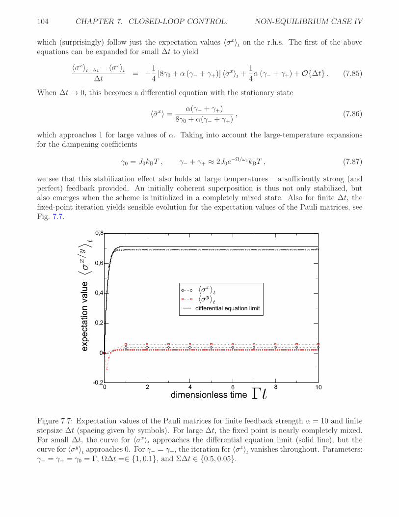
104 CHAPTER 7. CLOSED-LOOP CONTROL: NON-EQUILIBRIUM CASE IV
which (surprisingly) follow just the expectation values 〈σx〉t on the r.h.s. The first of the aboveequations can be expanded for small ∆t to yield
〈σx〉t+∆t − 〈σx〉t∆t
= −1
4[8γ0 + α (γ− + γ+)] 〈σx〉t +
1
4α (γ− + γ+) +O∆t . (7.85)
When ∆t → 0, this becomes a differential equation with the stationary state
〈σx〉 = α(γ− + γ+)
8γ0 + α(γ− + γ+), (7.86)
which approaches 1 for large values of α. Taking into account the large-temperature expansionsfor the dampening coefficients
γ0 = J0kBT , γ− + γ+ ≈ 2J0e−Ω/ωckBT , (7.87)
we see that this stabilization effect also holds at large temperatures – a sufficiently strong (andperfect) feedback provided. An initially coherent superposition is thus not only stabilized, butalso emerges when the scheme is initialized in a completely mixed state. Also for finite ∆t, thefixed-point iteration yields sensible evolution for the expectation values of the Pauli matrices, seeFig. 7.7.
0 2 4 6 8 10
dimensionless time
-0,2
0
0,2
0,4
0,6
0,8
expe
cta
tion
va
lue
differential equation limit
Figure 7.7: Expectation values of the Pauli matrices for finite feedback strength α = 10 and finitestepsize ∆t (spacing given by symbols). For large ∆t, the fixed point is nearly completely mixed.For small ∆t, the curve for 〈σx〉t approaches the differential equation limit (solid line), but thecurve for 〈σy〉t approaches 0. For γ− = γ+, the iteration for 〈σz〉t vanishes throughout. Parameters:γ− = γ+ = γ0 = Γ, Ω∆t =∈ 1, 0.1, and Σ∆t ∈ 0.5, 0.05.