non-equilibrium phase transitions -...

LECTURE NOTES

Non-equilibrium phase transitions

Haye Hinrichsen

Fakultat fur Physik und Astronomie, Universitat Wurzburg,

D–97074 Wurzburg, Germany

E-mail: [email protected]

Lectures held at the

International Summer School on

Problems in Statistical Physics XI

Leuven, Belgium, September 2005

Abstract: These lecture notes give a basic introduction to the physics of phase

transitions under non-equilibrium conditions. The notes start with a general

introduction to non-equilibrium statistical mechanics followed by four parts.

The first one discusses the universality class of directed percolation, which

plays a similar role as the Ising model in equilibrium statistical physics. The

second one gives an overview about other universality classes which have been

of interest in recent years. The third part extends the scope to models with

long-range interactions, including memory effects and so-called Levy flights.

Finally, the fourth part is concerned with deposition-evaporation phenomena

leading to wetting transitions out of equilibrium.

Contents

1 Introduction 2

1.1 Master equation . . . . . . . . . . . . . . . . 2

1.2 Equilibrium dynamics . . . . . . . . . . . . . 3

1.3 Non-equilibrium dynamics . . . . . . . . . . . 4

1.4 Non-equilibrium phase transitions . . . . . . . 5

2 Directed percolation 6

2.1 Directed bond percolation on a lattice . . . . 6

2.2 Absorbing states and critical behavior . . . . 9

2.3 The Domany-Kinzel cellular automaton . . . 12

2.4 The contact process . . . . . . . . . . . . . . 15

2.5 The critical exponents β, β′, ν⊥, and ν‖ . . . 16

2.6 Scaling laws . . . . . . . . . . . . . . . . . . . 17

2.7 Universality . . . . . . . . . . . . . . . . . . . 18

2.8 Langevin equation . . . . . . . . . . . . . . . 19

2.9 Multifractal properties of currents on di-rected percolation clusters . . . . . . . . . . . 19

2.10 Characterizing non-equilibrium transition byYang-Lee zeroes in the complex plane . . . . 21

3 Other classes of absorbing phase transitions 223.1 Parity-conserving particle processes . . . . . . 223.2 The voter universality class . . . . . . . . . . 233.3 Absorbing phase transitions with a con-

served field . . . . . . . . . . . . . . . . . . . 253.4 The diffusive pair contact process . . . . . . . 25

4 Epidemic spreading with long-range interac-tions 274.1 Immunization and mutations . . . . . . . . . 284.2 Long-range infections . . . . . . . . . . . . . . 284.3 Incubation times . . . . . . . . . . . . . . . . 29

5 Surface growth and non-equilibrium wetting 30

6 Summary 31

References 32

Non-equilibrium phase transitions 2

1. Introduction

This lecture is concerned with classical stochastic many-particle systems far away fromthermal equilibrium. Such systems are used as models of a much more complex physicalreality with many degrees of freedom in which chaotic or quantum-mechanical effectslead effectively to a classical random dynamics on a coarse-grained scale.

In order to explain the notion of stochastic non-equilibrium systems, let us forexample consider an experimental setup of molecular beam epitaxy. On a fundamentallevel a freshly deposited diffusing atom is described by a quantum-mechanical wavefunction that evolves under the influence of various interactions with the substrate andthe environment. However, monitoring the particle by modern imaging techniques,it seems to behave as a classical object that hops occasionally from one lattice siteto the other. In fact, in contrast to isolated quantum-mechanical particles, whosewave packages spread in time, the deposited atom is exposed to a complex varietyof interactions and entanglements with the environment which lead to a continuousdecoherence of the quantum state [1]. This process of decoherence keeps the wavepackage localized and thereby pinned to a certain lattice site as time proceeds. Theopposing quantum effect of recoherence, however, leads to occasional tunneling throughthe surrounding energy barriers. Immediately after tunneling, decoherence againlocalizes the wave function at the target site, destroying all information encoded inquantum-mechanical phases. This means that several subsequent tunneling events areeffectively uncorrelated, provided that they are separated by time intervals that are muchlarger than the typical decoherence time. It is this separation of time scales that allowsone to consider the particle as a classical object that evolves in time by spontaneousuncorrelated random moves to neighboring sites. Using this classical picture it is nolonger necessary to consider the full wave function of the particle, rather it is sufficientto characterize its state by the index of the lattice site to which it is pinned at timet and the effective transition rates by which it hops to its nearest neighbors. Thisinterpretation can be extended to chemical reactions as well.

1.1. Master equation

More generally, a classical stochastic many-particle system is defined by a set Cof possible configurations of the particles c ∈ C. The process evolves in time byinstantaneous transitions c → c′ which occur spontaneously like in a radioactive decaywith certain rates wc→c′ ≥ 0. The set of all configurations, the transition rates and theinitial state fully define the stochastic model under consideration.

From the theoretical point of view an important object to study is the probabilityPt(c) to find the system at time t in a certain configuration c. Obviously this probabilitydistribution has to be normalized, i.e.,

∑

c Pt(c) = 1. While the evolution of the system’sconfiguration is generally unpredictable due to its stochastic nature, the temporalevolution of the probability distribution Pt(c) is predictable and given by a linear systemof differential equations. This system of equations, usually called master equation,describes the flow of probability between different configurations in terms of gain and


loss contributions:

∂

∂tPt(c) =

∑

c′wc′→cPt(c

′)

︸︷︷︸

gain

−∑

c′wc→c′Pt(c)

︸︷︷︸

loss

. (1)

The gain and loss terms balance one another so that the probability distribution remainsnormalized as time proceeds. It is important to note that the coefficients wc→c′ are rates

rather than probabilities and carry the unit [time]−1. Therefore, rates may be largerthan 1 and can be rescaled by changing the time scale.

In a more compact form this set of equation may be written as

∂t|Pt〉 = −L|Pt〉 , (2)

where |Pt〉 denotes a vector whose entries are the probabilities Pt(c). This meansthat the corresponding vector space has a dimension equal to the number of possibleconfigurations. The so-called Liouville operator L generates the temporal evolution andis defined in the canonical configuration basis by the matrix elements

〈c′|L|c〉 = −wc→c′ + δc,c′∑

c′′wc→c′′. (3)

A formal solution of this first-order differential equation is given by |Pt〉 = exp(−Lt)|P0〉,where |P0〉 denotes the initial probability distribution at t = 0. This means that |Pt〉can be expressed as a sum over exponentially varying eigenmodes.

Since most stochastic processes are irreversible and therefore not invariant undertime reversal, the Liouville operator L is generally non-hermitean. However, the formof L is restricted by the requirements of the aforementioned balance between gain andloss terms as well as by the positivity of the rates. In the mathematical literature suchmatrices are usually called intensity matrices, meaning that all diagonal (off-diagonal)entries are real and positive (negative) and that the sum over each column of the matrixvanishes. The eigenvalues of an intensity matrix may be complex, indicating oscillatorybehavior, but their real part is always non-negative. Moreover, probability conservationensures that the spectrum includes at least one zero mode L|Ps〉 = 0, representingthe stationary probability distribution of the system. The other eigenvalues withpositive real parts represent relaxational eigenmodes which decay exponentially withtime. Therefore, if all other eigenvalues have strictly positive real parts, a stochasticprocess with a finite configuration space approaches a well-defined stationary probabilitydistribution P∞(c) exponentially.

1.2. Equilibrium dynamics

Equilibrium statistical mechanics is based on the axiom that the underlying quantum-mechanical laws are built in such a way that an isolated stochastic system in itsstationary state maximizes entropy. This means that it evolves through the accessibleconfigurations with the same probability, forming a microcanonical ensemble. In mostapplications, however, the stochastic system is not isolated but coupled to an external


heat bath. A heat bath is a surrounding environment consisting of many degrees offreedom that exchanges energy with the system of interest. For example, in molecularbeam epitaxy the deposited particle interacts with the phonons of the substrate by anexchange of energy, i.e., the substrate provides a thermal heat bath. Assuming that thecombination of system and heat bath maximizes entropy while conserving energy it iseasy to show that the stationary probability distribution Peq(c) is no longer uniform butgiven by the Boltzmann ensemble

Peq(c) =1

Zexp(−E(c)/kBT ) , (4)

where T is the temperature of the heat bath and Z is the partition sum over all accessibleconfigurations. Therefore, in equilibrium statistical mechanics it is not necessary to solvea partial differential equation, instead the stationary distribution is delivered for free.

Equilibrium models are fully defined by the accessible configurations c ∈ C and thecorresponding energies E(c). Although the Boltzmann ensemble renders the stationarydistribution for free it does not provide any information about relaxational modes.Consequently, the dynamical rules for a given equilibrium system in terms of transitionrates are not unique. In fact, as the only requirement the stationary zero mode ofthe Liouville operator has to reproduce the Boltzmann ensemble, which determines thematrix elements of L only partially. This is the reason why the well-known Ising modelcan be simulated on a computer by various dynamical algorithms, including heat bath,Glauber, Metropolis, and Swendsen-Wang dynamics. All these dynamical processesrelax towards the same stationary state that reproduces the Boltzmann ensemble of theIsing model. However, their dynamical properties can be quite different which plays animportant role with respect to critical slowing down in the vicinity of a phase transition.

Constructing dynamical rules that reproduce the stationary distribution of a givenequilibrium model, it is always possible to choose the transition rates in such a way thatthey obey detailed balance, i.e.

Peq(c)wc→c′ = Peq(c′)wc′→c . (5)

This means that the probability currents between pairs of configurations c and c′ canceleach other, as sketched in the left panel of Fig. 1.

1.3. Non-equilibrium dynamics

Dynamical systems are said to be out of equilibrium if the microscopic processes violatedetailed balance. Roughly speaking, the term “non-equilibrium” refers to situationswhere the probability currents between microstates do not vanish. For example, anGlauber-Ising model that has not yet reached the stationary state violates detailedbalance and hence is out of equilibrium. But even systems in a stationary state canbe out of equilibrium. Let us, for example, consider a system with three configurationsA,B,C that hops clockwise by cyclic transition rates wA→B = wB→C = wC→A = 1 (seeright panel of Fig. 1). This process quickly approaches a stationary state with equalprobabilities Ps(A) = Ps(B) = Ps(C) = 1/3. Although this stationary distribution


A B

C

A B

C

Figure 1. Detailed balance and non-equilibrium steady states. The figure sketches

a hypothetical system with three microstates A, B, C. In both cases the stationary

distribution function is Ps(A) = Ps(B) = Ps(C) = 1/3. Left: The transitions occur

at equal rates in all directions, hence the effective probability currents vanish and the

dynamics obeys detailed balance. Right: The transitions occur only clockwise, leading

to non-vanishing probability currents. Consequently, even the stationary state of the

system is out of equilibrium.

corresponds to a Boltzmann distribution with constant energy, the process violates thecondition of detailed balance and is therfore out of equilibrium.

On a more hand-waving level all systems subjected to external currents such asexternal driving or supply of energy or particles are expected to be out of equilibrium.For example, a running steam engine, although working in a stationary situation, needscontinuous supply of air, coal, and water, hence it is in principle impossible to establishdetailed balance. Nevertheless a steam engine is still close to equilibrium, meaning thaton certain scales the processes are almost thermalized so that the concepts of equilibriumphysics can still be applied.

In this lecture, we are primarily interested in systems far from equilibrium. Tothis end we consider stochastic processes that violate detailed balance so stronglythat concepts of equilibrium statistical physics can no longer be applied, even in anapproximate sense. We are interested in the question whether stochastic processes farfrom equilibrium can exhibit new phenomena that cannot be observed under equilibriumconditions. This applies in particular to phase transitions far from equilibrium.

1.4. Non-equilibrium phase transitions

Particularly interesting in classical stochastic systems are situations in which themicroscopic degrees of freedom behave collectively over large scales [2,3], especially whenthe system undergoes a continuous phase transition. In equilibrium statistical mechanicsthe best known example is the order-disorder transition in the two-dimensionalIsing model, where the typical size of ordered domains diverges when the criticaltemperature Tc is approached. It is well known that in second-order phase transitionat thermal equilibrium the emerging long-range correlations are fully specified by thesymmetry properties of the model under consideration and do not depend on detailsof the microscopic interactions. This allows one to associate these transitions withdifferent universality classes. The notion of universality was originally introduced byexperimentalists in order to describe the observation that several apparently unrelatedphysical systems are sometimes characterized by the same type of singular behaviornear the transition. Since then the concept of universality classes became a paradigm


of statistical physics. As the number of such classes seems to be limited, the aim oftheoretical statistical mechanics would be to provide a complete classification scheme.The most remarkable breakthrough in this direction was the application of conformalfield theory to equilibrium critical phenomena [4–6], leading to an extremely powerfulclassification scheme of continuous phase transitions in two dimensions.

Continuous phase transitions far away from equilibrium are less well understood.It turns out that the concept of universality, which has been very successful in the fieldof equilibrium critical phenomena, can be applied to non-equilibrium phase transitionsas well. However, the universality classes of non-equilibrium critical phenomena areexpected to be even more diverse as they involve time as an extra degree of freedomand are therefore governed by various symmetry properties of the evolution dynamics.Obviously, there is a large variety of phenomenological non-equilibrium phase transitionsin Nature, ranging for example from morphological transitions of growing surfaces [7]to traffic jams [8]. On the other hand, the experimental evidence for universality ofnon-equilibrium phase transitions is still very poor, calling for intensified experimentalefforts.

One important class of non-equilibrium phase transitions, on which we will focus inthis lecture, occurs in models with so-called absorbing states, i.e., configurations that canbe reached by the dynamics but cannot be left. The most prominent universality classof absorbing-state transitions is directed percolation (DP) [9]. This type of transitionoccurs, for example, in models for the spreading of infectious diseases. Amazingly, DPis one of very few critical phenomena which cannot be solved exactly in one spatialdimension. Although DP is easy to define, its critical behavior is highly nontrivial.This is probably one of the reasons why DP keeps theoretical physicists fascinated.

Moreover, these lecture notes discuss various other classes of non-equilibriumphase transitions and give a short introduction to wetting far from equilibrium. Thepresentation is based on various existing sources, in particular on the book by Marroand Dickman [10] and the review articles by Kinzel [9], Grassberger [11], Odor [12],Lubeck [13], and myself [14]. The reader is also referred to a large number of researcharticles for further reading.

2. Directed percolation

The probably most important class of non-equilibrium processes, which display a non-trivial phase transition from a fluctuating phase into an absorbing state, is Directed

Percolation (DP). As will be discussed below, the DP class comprises a large variety ofmodels that share certain basic properties.

2.1. Directed bond percolation on a lattice

To start with let us first consider a specific model called directed bond percolation whichis often used as a simple model for water percolating through a porous medium. Themodel is defined on a tilted square lattice whose sites represent the pores of the medium.The pores are connected by small channels (bonds) which are open with probability pand closed otherwise. As shown in Fig. 2, water injected into one of the pores will


isotropic percolation directed percolation

Figure 2. Isotropic versus directed bond percolation. The figure shows two identical

realizations of open and closed bonds on a finite part of a tilted square lattice. A

spreading agent (red) is injected at the central site (blue circle). In the case of isotropic

percolation (left) the agent percolates through open bonds in any direction. Contrarily,

in the case of directed percolation, the agent is restricted to percolate along a preferred

direction, as indicated by the arrow.

percolate along open channels, giving rise to a percolation cluster of wetted pores whoseaverage size will depend on p.

There are two fundamentally different versions of percolation models. In isotropic

percolation the flow is undirected, i.e., the spreading agent (water) can flow in anydirection through open bonds (left panel of Fig. 2). A comprehensive introduction toisotropic percolation is given in the textbook by Stauffer [15]. In the present lecture,however, we are primarily interested in the case of directed percolation. Here the clustersare directed, i.e., the water is restricted to flow along a preferred direction in space, asindicated by the arrow in Fig. 2. In the context of porous media this preferred directionmay be interpreted as a gravitational driving force. Using the language of electroniccircuits DP may be realized as a random diode network (cf. Sect. 2.9).

The strict order of cause and effect in DP allows one to interpret the preferreddirection as a temporal coordinate. For example, in directed bond percolation, we mayenumerate horizontal rows of sites by an integer time index t (see Fig. 3). Instead of astatic model of directed connectivity, we shall from now on interpret DP as a dynamicalprocess which evolves in time. Denoting wetted sites as active and dry sites as inactive

the process starts with a certain initial configuration of active sites that can be chosenfreely. For example, in Fig. 3 the process starts with a single active seed at the origin.As t increases the process evolves stochastically through a sequence of configurationsof active sites, also called states at time t. An important quantity, which characterizesthese intermediate states, is the total number of active sites N(t), as illustrated in Fig. 3.

Regarding directed percolation as a reaction-diffusion process the local transitionrules may be interpreted as follows. Each active site represents a particle A. If thetwo subsequent bonds are both closed, the particle will have disappeared at the nexttime step by a death process A → ∅ (see Fig. 4a). If only one of the bonds is open,


7

6

5

4

3

2

1

0 1

1

2

1

2

2

3

2

t N(t)seed

time

Figure 3. Directed bond percolation. The process shown here starts with a single

active seed at the origin. It then evolves through a sequence of configurations along

horizontal lines (called states) which can be labeled by a time-like index t. An

important quantity to study would be the total number of active sites N(t) at time t.

a) b) c) d) e)

Figure 4. Interpretation of the dynamical rules of directed bond percolation as a

reaction-diffusion process: a) death process, b)-c) diffusion, d) offspring production,

and e) coagulation.

the particle diffuses stochastically to the left or to the right, as shown in Fig. 4b-4c.Finally, if the two bonds are open the particles creates an offspring A → 2A (Fig. 4d).However, it is important to note that each site in directed bond percolation can be eitheractive or inactive. In the particle language this means that each site can be occupiedby at most one particle. Consequently, if two particles happen to reach the same site,they merge irreversibly forming a single one by coalescence 2A → A, as illustrated inFig. 4e. Summarizing these reactions, directed bond percolation can be interpreted asa reaction-diffusion process which effectively follows the reaction scheme

A→ ∅ death process

A→ 2A offspring production (6)

2A→ A coagulation

combined with single-particle diffusion.

The dynamical interpretation in terms of particles is of course the natural languagefor any algorithmic implementation of DP on a computer. As the configuration at time tdepends exclusively on the previous configuration at time t − 1 it is not necessary tostore the entire cluster in the memory, instead it suffices to keep track of the actualconfiguration of active sites at a given time and to update this configuration in parallelsweeps according to certain probabilistic rules. In the case of directed bond percolation,one obtains a stochastic cellular automaton with certain update rules in which eachactive site of the previous configuration activates its nearest neighbors of the actualconfiguration with probability p. In fact, as shown in Fig. 5, a simple non-optimized


t

i

//============== Simple C-code for directed percolation =============

#include <fstream.h>

using namespace std;

const int T=1000; // number of rows

const int R=10000; // number of runs

const double p=0.7; // percolation probability

int N[T]; // cumulative occupation number

//--- random number generator returning doubles between 0 and 1 -----

inline double rnd(void) { return (double)rand()/0x7FFFFFFF; }

//------------ construct directed percolation cluster ---------------

void DP (void) {

int t,i,s[T][T]; // static array

for (t=0;t<T;t++) for (i=0;i<=t;i++) s[t][i]=0; // clear lattice

s[0][0]=1; // place seed

// perform loop over all active sites:

for (t=0; t<T-1; t++) for (i=0; i<=t; i++) if (s[t][i]) {

N[t]++;

if (rnd()<p) s[t+1][i]=1; // offspring right

if (rnd()<p) s[t+1][i+1]=1; // offspring left

}

}

//-------- perform R runs and write average N(t) to disk -----------

int main (void) {

for (int t=0; t<T; t++) N[t]=0; // reset N(t)

for (int r=0; r<R; r++) DP(); // perform R runs

ofstream os("N.dat"); // write result to disk

for (int t=0; t<T-1; t++) os << t << "\t" << (double)N[t]/R << endl;

}

Figure 5. Simple non-optimized program in C for directed bond percolation. The

numerical results are shown below in Fig. 6.

C-code for directed bond percolation takes less than a page, and the core of the updaterules takes only a few lines.

2.2. Absorbing states and critical behavior

As only active sites at time t can activate sites at time t+ 1, the configuration without

active sites plays a special role. Obviously, such a state can be reached by the dynamicsbut it cannot be left. In the literature such states are referred to as absorbing. Absorbing


i

t

i

t

i

t

p<p c cc p=p p>p

Figure 6. Typical DP clusters in 1+1 dimensions grown from a single seed below, at,

and above criticality.

states can be thought of as a trap: Once the system reaches the absorbing state itbecomes trapped and will stay there forever. As we will see below, a key feature ofdirected percolation is the presence of a single absorbing state, usually represented bythe empty lattice.

The mere existence of an absorbing state demonstrates that DP is a dynamicalprocess far from thermal equilibrium. As explained in the Introduction, equilibriumstatistical mechanics deals with stationary equilibrium ensembles that can be generatedby a dynamics obeying detailed balance, meaning that probability currents between pairsof sites cancel each other. As the absorbing state can only be reached but not be left,there is always a non-zero current of probability into the absorbing state that violatesdetailed balance. Consequently the temporal evolution before reaching the absorbingstate cannot be described in terms of thermodynamic ensembles, proving that DP is anon-equilibrium process.

The enormous theoretical interest in DP – more than 800 articles refer to this class ofmodels – is related to the fact that DP displays a non-equilibrium phase transition froma fluctuating phase into the absorbing state controlled by the percolation probability p.The existence of such a transition is quite plausible since offspring production andparticle death compete with each other. As will be discussed below, phase transitionsinto absorbing states can be characterized by certain universal properties which areindependent of specific details of the microscopic dynamics. In fact, the term ‘directedpercolation’ does not stand for a particular model, rather it denotes a whole universalityclass of models which display the same type of critical behavior at the phase transition.The situation is similar as in equilibrium statistical mechanics, where for example theIsing universality class comprises a large variety of different models. In fact, DP isprobably as fundamental in non-equilibrium statistical physics as the Ising model inequilibrium statistical mechanics.

In DP the phase transition takes place at a certain well-defined critical percolationprobability pc. As illustrated in Fig. 6 the behavior on both sides of pc is very different.In the subcritical regime p < pc any cluster generated from a single seed has a finitelife time and thus a finite mass. Contrarily, in the supercritical regime p > pc thereis a finite probability that the generated cluster extends to infinity, spreading roughlywithin a cone whose opening angle depends on p−pc. Finally, at criticality finite clustersof all sizes are generated. These clusters are sparse and remind of self-similar fractal


1 10 100 1000t

0,01

0,1

1

10

100

<N

(t)>

p=0.7p=0.65p=0.6447 (critical)p=0.64p=0.6

0 100 300 400t10

-2

10-1

100

<N

(t)>

Figure 7. Directed bond percolation: Number of particles N(t) as a function of time

for different values of the percolation probability p. The critical point is characterized

by an asymptotic power law behavior. The inset demonstrates the crossover to an

exponential decay in the subcritical phase for p = 0.6.

objects. As we will see, a hallmark of such a scale-free behavior is a power-law behaviorof various quantities.

The precise value of the percolation threshold pc is non-universal (i.e., it dependson the specific model) and can only be determined numerically. For example, inthe case of directed bond percolation in 1+1 dimensions, the best estimate is pc =0.644700185(5) [16]. Unlike isotropic bond percolation in two dimensions, where thecritical value is exactly given by piso

c = 1/2, an analytical expression for the criticalthreshold of DP in finite dimensions is not yet known. This seems to be related to thefact that DP is a non-integrable process. It is in fact amazing that so far, in spite of itssimplicity and the enormous effort by many scientists, DP resisted all attempts to besolved exactly, even in 1+1 dimensions.

In order to describe the phase transition quantatively an appropriate orderparameter is needed. For simulations starting from a single active seed a suitable orderparameter is the average number of particles 〈N(t)〉 at time t, where 〈. . .〉 denotes theaverage over many independent realizations of randomness (called runs in the numericaljargon). For example, the program shown in Fig. 5 averages this quantity over 10.000runs and stores the result in a file that can be viewed by a graphical tool such asxmgrace. As shown in Fig. 7, there are three different cases:

• For p < pc the average number of active sites first increases and then decreasesrapidly. As demonstrated in the inset, this decrease is in fact exponential. Obvi-ously, the typical crossover time, where exponential decay starts, depends on thedistance from criticality pc − p.


• At criticality the average number of active sites increases according to a power law〈N(t)〉 ∼ tθ. A standard regression of the data gives the exponent θ ≃ 0.302, shownin the figure as a thin dashed line. As can be seen, there are deviations for low t,i.e., the process approaches a power-law only asymptotically.

• In the supercritical regime p > pc the slow increase of 〈N(t)〉 crosses over to a fastlinear increase with time. Again the crossover time depends on the distance fromcriticality p− pc.

The properties of 〈N(t)〉 above and below criticality can be used to determine thecritical threshold numerically. This iterative procedure works as follows: Starting witha moderate simulation time it is easy to specify a lower and an upper bound for pc byhand, e.g., 0.64 < pc < 0.65 in the case of directed bond percolation. This intervalis then divided into two equal parts and the process is simulated in between, e.g., atp = 0.645. In order to find out whether this value is sub- or supercritical one has tocheck deviations for large t from a straight line in a double logarithmic plot. If the curveveers down (up) the procedure is iterated using the upper (lower) interval. In detectingthe sign of curvature the human eye is quite reliable but it is also possible to recognize itautomatically. If there is no obvious deviation from a straight line the simulation timeand the number of runs has to be increased appropriately.

Warning: Determining the numerical error for the estimate of a critical exponentnever use the statistical χ2-error of a standard regression! For example, for the dataproduced by the minimal program discussed above, a linear regression by xmgrace wouldgive the result θ = 0.3017(2). However, the estimate in the literature θ = 0.313686(8)lies clearly outside these error margins, meaning that the actual error must be muchhigher. A reliable estimate of the error can be obtained by comparing the slopes overthe last decade of simulations performed at the upper and the lower bound of pc.

In principle the accuracy of this method is limited only by the available CPU time.We note, however, that this standard method assumes a clean asymptotic power lawscaling, which for DP is indeed the case. However, in some cases the power law maybe superposed by slowly varying deviations, e.g. logarithmic corrections, so that theplotted data at criticality is actually not straight but slightly curved. With the methodoutlined above one is then tempted to ‘compensate’ this curvature by tuning the controlparameter, leading to unknown systematic errors. Recently this happened, for example,in the case of the diffusive pair contact process, as will be described in Sect. 3.4.

2.3. The Domany-Kinzel cellular automaton

An important model for DP, which includes directed bond percolation as a special case, isthe celebrated Domany-Kinzel model [17,18]. The Domany-Kinzel model is a stochasticcellular automaton defined on a diagonal square lattice which evolves by parallel updatesaccording to certain conditional transition probabilities P [si(t+1)|si−1(t), si+1(t)], wheresi(t) ∈ {0, 1} denotes the occupancy of site i at time t. These probabilities depend ontwo parameters p1, p2 and are defined by

P [1|0, 0] = 0 ,


0 1p

1

0

1

p2

inactive phase

activephase

compact DP

bond DP

site DP

W18

Figure 8. Phase diagram of the Domany-Kinzel model.

P [1|0, 1] = P [1|1, 0] = p1 , (7)

P [1|1, 1] = p2 ,

with P [0|·, ·] = 1 − P [1|·, ·]. On a computer the Domany-Kinzel model can beimplemented as follows. To determine the state si(t) of site i at time t we generatefor each site a random number z ∈ (0, 1) from a flat distribution and set

si(t+ 1) =

1 if si−1(t) 6= si+1(t) and zi(t) < p1 ,

1 if si−1(t) = si+1(t) = 1 and zi(t) < p2 ,

0 otherwise .

(8)

This means that a site is activated with probability p2 if the two nearest neighbors at theprevious time step were both active while it is activated with probability p1 if only oneof them was active. Thus the model depends on two percolation probabilities p1 and p2,giving rise to the two-dimensional phase diagram shown in Fig. 8. The active and theinactive phase are now separated by a line of phase transitions. This line includes severalspecial cases. For example, the previously discussed case of directed bond percolationcorresponds to the choice p1 = p and p2 = p(2−p). Another special case is directed sitepercolation [9], corresponding to the choice p1 = p2 = p. In this case all bonds are openbut sites are permeable with probability p and blocked otherwise. Finally, the specialcase p2 = 0 is a stochastic generalization of the rule ‘W18’ of Wolfram’s classificationscheme of cellular automata [19]. Numerical estimates for the corresponding criticalparameters are listed in Table 1.

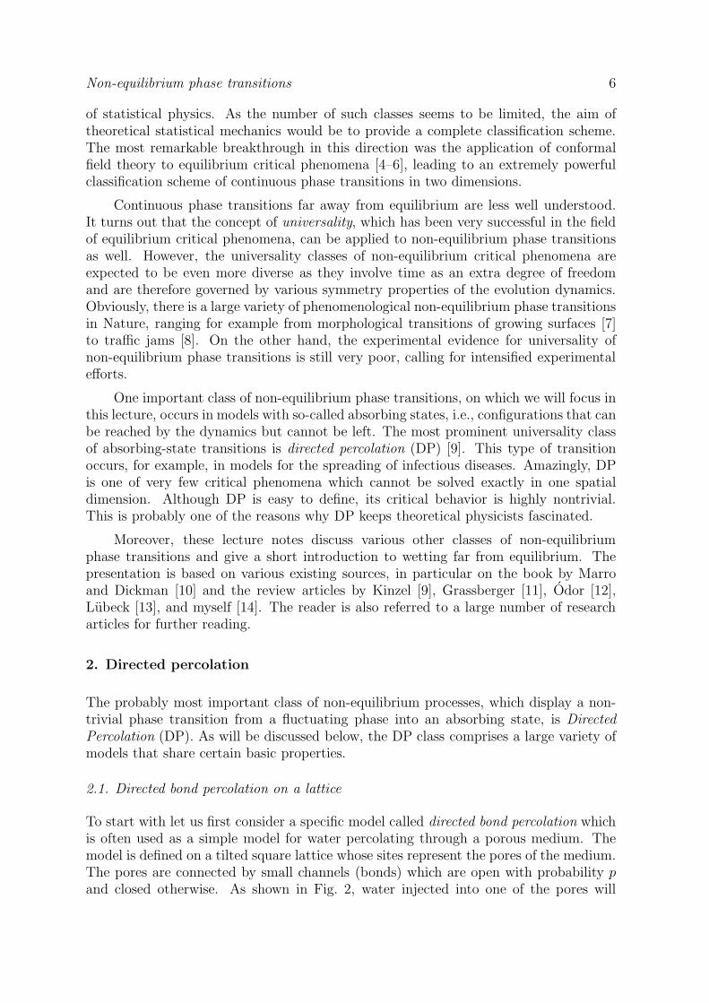
There is strong numerical evidence that the critical behavior along the wholephase transition line (except for its upper terminal point) is that of DP, meaning thatthe transitions always exhibit the same type of long-range correlations. The short-range correlations, however, are non-universal and may change when moving along thephase transition line. They may even change the visual appearance of the clusters,as illustrated in Fig. 9, where four typical snapshots of critical clusters are compared.


transition point p1,c p2,c Ref.

Wolfram rule 18 0.801(2) 0 [20]

site DP 0.70548515(20) 0.70548515(20) [16]

bond DP 0.644700185(5) 0.873762040(3) [16]

compact DP 1/2 1 [9]

Table 1. Special transition points in the (1+1)-dimensional Domany-Kinzel model.

site DP bond DP compact DPWolfram 18

Figure 9. Domany-Kinzel model: Critical cluster generated from a single active seed

at different points along the phase transition line (see text).

Although the large-scale structure of the clusters in the first three cases is roughly thesame, the microscoppic texture seems to become bolder as we move up along the phasetransition line. As shown in Ref. [14], this visual impression can be traced back to anincrease of the mean size of active islands.

Approaching the upper terminal point the mean size of active islands diverges andthe cluster becomes compact. For this reason this special point is usually referred toas compact directed percolation. However, this nomenclature may be misleading forthe following reasons. The exceptional behavior at this point of is due to an additionalsymmetry between active and inactive sites along the upper border of the phase diagramat p2 = 1. Here the DK model has two symmetric absorbing states, namely, the emptyand the fully occupied lattice. For this reason the transition does no longer belong tothe universality class of directed percolation, instead it becomes equivalent to the (1+1)-dimensional voter model [2, 21] or the Glauber-Ising model at zero temperature. Sincethe dynamic rules are invariant under the replacement p1 ↔ 1 − p1, the correspondingtransition point is located at p1 = 1/2.

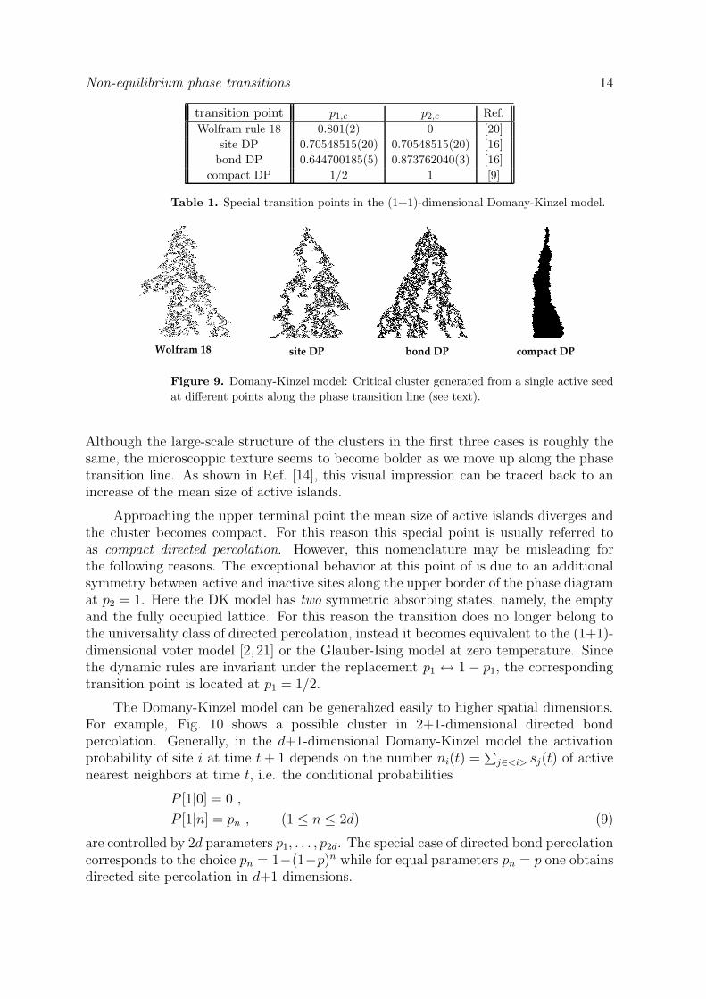
The Domany-Kinzel model can be generalized easily to higher spatial dimensions.For example, Fig. 10 shows a possible cluster in 2+1-dimensional directed bondpercolation. Generally, in the d+1-dimensional Domany-Kinzel model the activationprobability of site i at time t+ 1 depends on the number ni(t) =

∑

j∈<i> sj(t) of activenearest neighbors at time t, i.e. the conditional probabilities

P [1|0] = 0 ,

P [1|n] = pn , (1 ≤ n ≤ 2d) (9)

are controlled by 2d parameters p1, . . . , p2d. The special case of directed bond percolationcorresponds to the choice pn = 1−(1−p)n while for equal parameters pn = p one obtainsdirected site percolation in d+1 dimensions.


t

Figure 10. Lattice geometry of directed bond percolation in 2+1 dimensions. The

red lines represent a possible cluster generated at the origin.

2.4. The contact process

Another important model for directed percolation, which is popular in mathematicalcommunities, is the contact process. The contact process was originally introducedby Harris [22] as a model for epidemic spreading (see Sect. 4). It is defined on ad-dimensional square lattice whose sites can be either active (si(t) = 1) or inactive(si(t) = 0). In contrast to the Domany-Kinzel model, which is a stochastic cellularautomaton with parallel updates, the contact process evolves by asynchronous updates,i.e., the three elementary processes (offspring production, on-site removal and diffusivemoves) occur spontaneously at certain rates. Although the microscopic dynamics differssignificantly from the Domany-Kinzel model, the contact process displays the sametype of critical behavior at the phase transition. In fact, both models belong to theuniversality class of DP.

On a computer the d+1-dimensional contact process can be implemented as follows.For each attempted update a site i is selected at random. Depending on its state si(t)and the number of active neighbors ni(t) =

∑

j∈<i> sj(t) a new value si(t+ dt) = 0, 1 isassigned according to certain transition rates w[si(t) → si(t+dt), ni(t)]. In the standardcontact process these rates are defined by

w[0 → 1, n] = λn/2d , (10)

w[1 → 0, n] = 1 . (11)

Here the parameter λ plays the same role as the percolation probability in directedbond percolation. Its critical value depends on the dimension d. For example, in 1+1dimensions the best-known estimate is λc ≃ 3.29785(8) [23].

As demonstrated in Ref. [14] the evolution of the contact process can be describedin terms of a master equation whose Liouville operator L can be constructed explicitelyon a finite lattice. Diagonalizing this operator numerically one obtains a spectrum ofrelaxational modes with at least one zero mode which represents the absorbing state.In the limit of large lattices the critical threshold λc is usually the point from where onthe first gap in the spectrum of L vanishes.


2.5. The critical exponents β, β ′, ν⊥, and ν‖

In equilibrium statistical physics, continuous phase transitions as the one in the Isingmodel can be described in terms of a phenomenological scaling theory. For example,the spontaneous magnetization M in the ordered phase vanishes as |M | ∼ (Tc − T )β asthe critical point is approached. Here β is a universal critical exponent, i.e. its value isindependent of the specific realization of the model. Similarly, the correlation length ξdiverges in as ξ ∼ |T −Tc|−ν for T → Tc with another universal exponent ν. The criticalpoint itself is characterized by the absence of a macroscopic length scale so that thesystem is invariant under suitable scaling transformations (see below).

In directed percolation and other non-equilibrium phase transitions into absorbingstates the situation is very similar. However, as non-equilibrium system involves timewhich is different from space in character, there are now two different correlation lengths,namely, a spatial correlation length ξ⊥ and a temporal correlation length ξ‖ with twodifferent associated exponents ν⊥ and ν‖. Their ratio z = ν‖/ν⊥ is called dynamical

exponent as it relates spatial and temporal scales at criticality.

What is the analogon of the magnetization in DP? As shown above, in absorbingphase transitions the choice of the order parameter depends on the initial configuration.If homogeneous initial conditions are used, the appropriate order parameter is thedensity of active sites at time t

ρ(t) = limL→∞

1

L

∑

i

si(t) . (12)

Here the density is defined as a spatial average in the limit of large system sizes L→ ∞.Alternatively, for a finite system with periodic boundary conditions we may express thedensity as

ρ(t) = 〈si(t)〉 , (13)

where 〈. . .〉 denotes the ensemble average over many realizations of randomness. Becauseof translational invariance the index i is arbitrary. Finally, if the process starts with asingle seed, possible order parameters are the average mass of the cluster

N(t) = 〈∑

i

si(t)〉 (14)

and the survival probability

P (t) = 〈1 −∏

i

(1 − si(t))〉 . (15)

These quantities allow us to define the four standard exponents

ρ(∞) ∼ (p− pc)β , (16)

P (∞) ∼ (p− pc)β′

, (17)

ξ⊥ ∼ |p− pc|−ν⊥ , (18)

ξ‖ ∼ |p− pc|−ν‖ . (19)


The necessity of two different exponents β and β ′ can be explained in the framework ofa field-theoretic treatment, where these exponents are associated with particle creationand annihilation operators, respectively. In DP, however, a special symmetry, calledrapidity reversal symmetry, ensures that β = β ′. This symmetry can be proven mosteasily in the case of directed bond percolation, where the density ρ(t) starting from afully occupied lattice and the survival probability P (t) for clusters grown from a seed areexactly equal for all t. Hence both quantities scale identically and the two correspondingexponents have to be equal. This is the reason why DP is characterized by only threeinstead of four critical exponents.

The cluster mass N(t) ∼ tθ scales algebraically as well. The associated exponent,however, is not independent, instead it can be expressed in terms of the so-calledgeneralized hyperscaling relation [24]

θ =dν⊥ − β − β ′

ν‖. (20)

In order to determine the critical point of a given model by numerical methods, N(t)turned out to be one of the most sensitive quantities.

2.6. Scaling laws

Starting point of a phenomenological scaling theory for absorbing phase transitions isthe assumption that the macroscopic properties of the system close to the critical pointare invariant under scaling transformations of the form

∆ → a∆, x → a−ν⊥x, t→ a−ν‖t, ρ→ aβρ, P → aβ′

P, (21)

where a > 0 is some scaling factor and ∆ = p− pc denotes the distance from criticality.Scaling invariance strongly restricts the form of functions. For example, let us considerthe decay of the average density ρ(t) at the critical point starting with a fully occupiedlattice. This quantity has to be invariant under rescaling, hence ρ(t) = aβρ(t a−ν‖).Choosing a such that t a−ν‖ = 1 we arrive at ρ(t) = t−β/ν‖ρ(1), hence

ρ(t) ∼ t−δ , δ = β/ν‖ . (22)

Similarly, starting from an initial seed, the survival probability Ps(t) decays as

Ps(t) ∼ t−δ′

, δ′ = β ′/ν‖ (23)

with δ = δ′ in the case of DP.

In an off-critical finite-size system, the density ρ(t,∆, L) and the survival probabilityP (t,∆, L) depend on three parameters. By a similar calculation it is easy to showthat scaling invariance always reduces the number of parameters by 1, expressing thequantity of interest by a leading power law times a scaling function that depends onscaling-invariant arguments. Such expressions are called scaling forms. For the densityand the survival probability these scaling forms read

ρ(t,∆, L) ∼ t−β/ν‖ f(∆ t1/ν‖ , td/z/L) , (24)

P (t,∆, L) ∼ t−β′/ν‖ f ′(∆ t1/ν‖ , td/z/L) . (25)


critical MF d = 1 d = 2 d = 3 d = 4 − ǫ

β 1 0.276486(8) 0.584(4) 0.81(1) 1 − ǫ/6 − 0.01128 ǫ2

ν⊥ 1/2 1.096854(4) 0.734(4) 0.581(5) 1/2 + ǫ/16 + 0.02110 ǫ2

ν‖ 1 1.733847(6) 1.295(6) 1.105(5) 1 + ǫ/12 + 0.02238 ǫ2

z 2 1.580745(10) 1.76(3) 1.90(1) 2 − ǫ/12− 0.02921 ǫ2

δ 1 0.159464(6) 0.451 0.73 1 − ǫ/4 − 0.01283 ǫ2

θ 0 0.313686(8) 0.230 0.12 ǫ/12 + 0.03751 ǫ2

Table 2. Critical exponents of directed percolation obtained by mean field (MF),

numerical, and field-theoretical methods.

2.7. Universality

As outlined in the introduction, the working hypothesis in the field of continuous non-equilibrium phase transitions is the notion of universality. This concept expresses theexpectation that the critical behavior of such transitions can be associated with a finiteset of possible universality classes, each corresponding to a certain type of underlyingfield theory. The field-theoretic action involves certain relevant operators whose form isusually determined by the symmetry properties of the process, while other details of themicroscopic dynamics lead to contributions which are irrelevant in the field-theoreticsense. This explains why various different models may belong to the same universalityclass.

In particular the DP class – the “Ising” class of non-equilibrium statistical physics –is extremely robust with respect to the microscopic dynamic rules. The large variety androbustness of DP models led Janssen and Grassberger to the conjecture that a modelshould belong to the DP universality class if the following conditions hold [25, 26]:

(i) The model displays a continuous phase transition from a fluctuating active phaseinto a unique absorbing state.

(ii) The transition is characterized by a positive one-component order parameter.

(iii) The dynamic rules involve only short-range processes.

(iv) The system has no unconventional attributes such as additional symmetries orquenched randomness.

Although this conjecture has not yet been proven rigorously, it is highly supported bynumerical evidence. In fact, DP seems to be even more general and has been identifiedeven in systems that violate some of the four conditions.

The universality classes can be characterized in terms of their critical exponentsand scaling functions. Hence in order to identify a certain universality class, a preciseestimation of the critical exponents is an important numerical task. In the case ofDP, the numerical estimates suggest that the critical exponents are given by irrational

numbers rather than simple rational values. In addition, scaling functions (such as fand f ′ in Eq. (24)), which were ignored in the literature for long time, provide a wealthof useful information, as shown e.g. in a recent review by Lubeck [13].


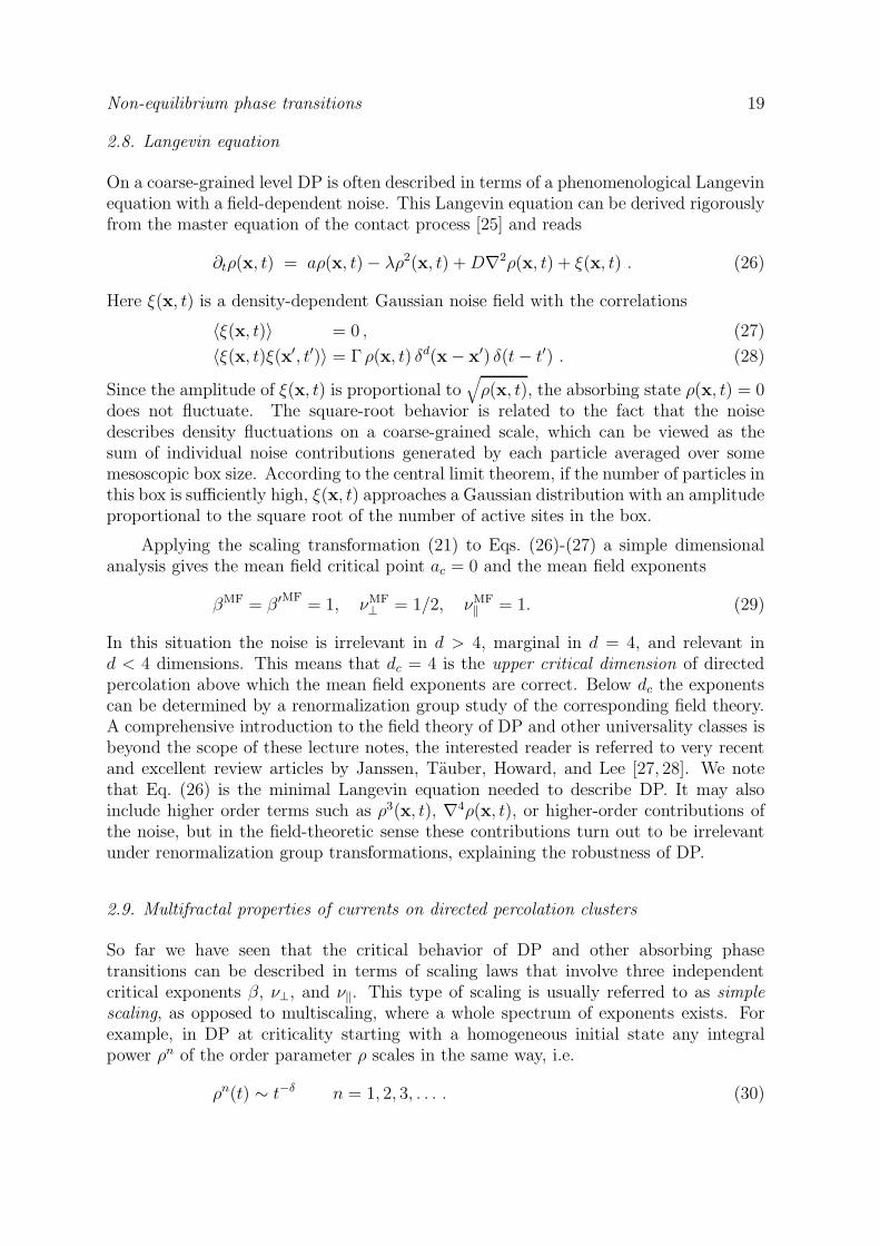
2.8. Langevin equation

On a coarse-grained level DP is often described in terms of a phenomenological Langevinequation with a field-dependent noise. This Langevin equation can be derived rigorouslyfrom the master equation of the contact process [25] and reads

∂tρ(x, t) = aρ(x, t) − λρ2(x, t) +D∇2ρ(x, t) + ξ(x, t) . (26)

Here ξ(x, t) is a density-dependent Gaussian noise field with the correlations

〈ξ(x, t)〉 = 0 , (27)

〈ξ(x, t)ξ(x′, t′)〉 = Γ ρ(x, t) δd(x − x′) δ(t− t′) . (28)

Since the amplitude of ξ(x, t) is proportional to√

ρ(x, t), the absorbing state ρ(x, t) = 0does not fluctuate. The square-root behavior is related to the fact that the noisedescribes density fluctuations on a coarse-grained scale, which can be viewed as thesum of individual noise contributions generated by each particle averaged over somemesoscopic box size. According to the central limit theorem, if the number of particles inthis box is sufficiently high, ξ(x, t) approaches a Gaussian distribution with an amplitudeproportional to the square root of the number of active sites in the box.

Applying the scaling transformation (21) to Eqs. (26)-(27) a simple dimensionalanalysis gives the mean field critical point ac = 0 and the mean field exponents

βMF = β ′MF= 1, νMF

⊥ = 1/2, νMF‖ = 1. (29)

In this situation the noise is irrelevant in d > 4, marginal in d = 4, and relevant ind < 4 dimensions. This means that dc = 4 is the upper critical dimension of directedpercolation above which the mean field exponents are correct. Below dc the exponentscan be determined by a renormalization group study of the corresponding field theory.A comprehensive introduction to the field theory of DP and other universality classes isbeyond the scope of these lecture notes, the interested reader is referred to very recentand excellent review articles by Janssen, Tauber, Howard, and Lee [27, 28]. We notethat Eq. (26) is the minimal Langevin equation needed to describe DP. It may alsoinclude higher order terms such as ρ3(x, t), ∇4ρ(x, t), or higher-order contributions ofthe noise, but in the field-theoretic sense these contributions turn out to be irrelevantunder renormalization group transformations, explaining the robustness of DP.

2.9. Multifractal properties of currents on directed percolation clusters

So far we have seen that the critical behavior of DP and other absorbing phasetransitions can be described in terms of scaling laws that involve three independentcritical exponents β, ν⊥, and ν‖. This type of scaling is usually referred to as simple

scaling, as opposed to multiscaling, where a whole spectrum of exponents exists. Forexample, in DP at criticality starting with a homogeneous initial state any integralpower ρn of the order parameter ρ scales in the same way, i.e.

ρn(t) ∼ t−δ n = 1, 2, 3, . . . . (30)


x

t

+ −U

I

Figure 11. Electric current running through a random resistor-diode network at the

percolation threshold from one point to the other. The right panel shows a particular

realization. The color and thickness of the line represent the intensity of the current.

Let us now consider an electric current running on a directed percolation clusteraccording to Kirchhoff’s laws, interpreting the cluster as a random resistor-diodenetwork. By introducing such a current the theory is extended by an additional physicalconcept. In fact, even though the DP cluster itself is known to be characterized by simplescaling laws, a current running on it turns out to be distributed in a multifractal manner.This phenomenon was first discovered in the case of isotropic percolation [29, 30] andthen confirmed for DP [31,32].

As shown in Fig. 11, in directed bond percolation at criticality an electric current Irunning from one point to the other is characterized by a non-trivial distribution ofcurrents. The multifractal structure of this current distribution can be probed bystudying the moments

Mℓ :=∑

b

(Ib/I)ℓ ℓ = 0, 1, 2, . . . , (31)

where the sum runs over all bonds b that transport a non-vanishing current Ib > 0.For example, M0 is just the number of conducting bonds while M1 is essentially thetotal resistance between the two points. M2 is the second cumulant of the resistancefluctuations and can be considered as a measure of the noise in a given realization.Finally, M∞ is the number of so-called red bonds that carry the full current I. Thequantity Mℓ is found to scale as a power law

Mℓ(t) ∼ tψℓ/ν‖ . (32)

In the case of simple scaling, the exponents ψℓ would depend linearly on ℓ. In thepresent case, however, a non-linear dependence is found both by field-theoretic as wellas numerical methods (see Ref. [32]). This proves that electric currents running on DPclusters have multifractal properties.

Again it should be emphasized that multifractality is not a property of DP itself,rather it emerges as a new feature whenever an additional process, here the transportof electric currents, is confined to live on the critical clusters of DP.


2.10. Characterizing non-equilibrium transition by Yang-Lee zeroes in the complex

plane

In equilibrium statistical mechanics a large variety of continuous phase transitions hasbeen analyzed by studying the distribution of so-called Yang-Lee zeros [33–35]. Todetermine these zeros the partition sum of a (finite) equilibrium system is expressed asa polynomial of the control parameter, which is usually a function of temperature. E.g.,for the Ising model the zeros of this polynomial lie on a circle in the complex plane andheckle the real line from both sides in the vicinity of the phase transition as the systemsize increases. This explains why the analytic behavior in finite system crosses over toa non-analytic behavior at the transition point in the thermodynamic limit.

Recently, it has been shown that the concept of Yang and Lee can also be appliedto non-equilibrium systems [36], including DP [37]. To this end one has to consider theorder parameter in a finite percolation tree as a function of the percolation probability pin the complex plane. This can be done by studying the survival probability P (t) (seeEq. (15)), which is defined as the probability that a cluster generated in a single site attime t = 0 survives at least up to time t. In fact, the partition sum of an equilibriumsystem and the survival probability of DP are similar in many respects. They bothare positive in the physically accessible regime and can be expressed as polynomials infinite systems. As the system size tends to infinity, both functions exhibit a non-analyticbehavior at the phase transition as the Yang-Lee zeros in the complex plane approachthe real line.

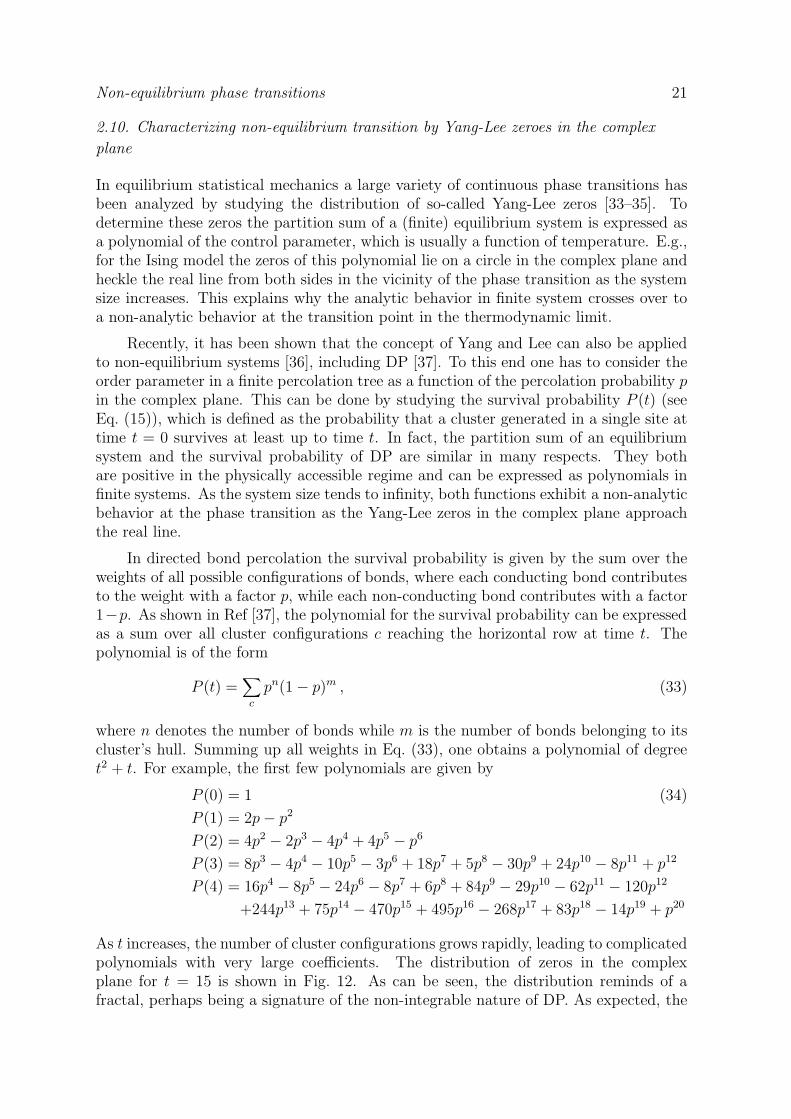
In directed bond percolation the survival probability is given by the sum over theweights of all possible configurations of bonds, where each conducting bond contributesto the weight with a factor p, while each non-conducting bond contributes with a factor1−p. As shown in Ref [37], the polynomial for the survival probability can be expressedas a sum over all cluster configurations c reaching the horizontal row at time t. Thepolynomial is of the form

P (t) =∑

c

pn(1 − p)m , (33)

where n denotes the number of bonds while m is the number of bonds belonging to itscluster’s hull. Summing up all weights in Eq. (33), one obtains a polynomial of degreet2 + t. For example, the first few polynomials are given by

P (0) = 1 (34)

P (1) = 2p− p2

P (2) = 4p2 − 2p3 − 4p4 + 4p5 − p6

P (3) = 8p3 − 4p4 − 10p5 − 3p6 + 18p7 + 5p8 − 30p9 + 24p10 − 8p11 + p12

P (4) = 16p4 − 8p5 − 24p6 − 8p7 + 6p8 + 84p9 − 29p10 − 62p11 − 120p12

+244p13 + 75p14 − 470p15 + 495p16 − 268p17 + 83p18 − 14p19 + p20

As t increases, the number of cluster configurations grows rapidly, leading to complicatedpolynomials with very large coefficients. The distribution of zeros in the complexplane for t = 15 is shown in Fig. 12. As can be seen, the distribution reminds of afractal, perhaps being a signature of the non-integrable nature of DP. As expected, the


-1 0 1 2 3 4Re(p)

-0,5

0

0,5

Im(p

)

criticalpoint

Figure 12. Distribution of Yang-Lee zeros of the polynomial P (15) in the complex

plane. The transition point is marked by an arrow.

zeros approach the phase transition point from above and below. Their distance to thetransition point is found to scale as t−1/ν‖ in agreement with basic scaling arguments.

3. Other classes of absorbing phase transitions

So far we discussed directed percolation as the most important class of non-equilibriumphase transitions into absorbing states. Because of the robustness of DP it is interestingto search for other universality classes. The ultimate goal would be to set up a table ofpossible non-trivial universality classes from active phases into absorbing states.

Although various exceptions from DP have been identified, the number of firmlyestablished universality classes is still small. A recent summary of the status quo canbe found in Refs. [12,13]. In these lecture notes, however, we will only address the mostimportant classes with local interactions.

3.1. Parity-conserving particle processes

The parity-conserving (PC) universality class comprises phase transitions that occur inreaction-diffusion processes of the form

A→ (n+ 1)A

2A→ ∅ (35)

(36)

combined with single-particle diffusion, where the number of offspring n is assumedto be even. As an essential feature, these processes conserve the number of particlesmodulo 2. A particularly simple model in this class with n = 2 was proposed by Zhong


Glauber−Ising model at T=0 Classical voter model

Figure 13. Coarsening of a random initial state in the Glauber-Ising model at zero

temperature compared to the coarsening in the classical voter model.

and ben-Avraham [38]. The estimated critical exponents

β = β ′ = 0.92(2) , ν‖ = 3.22(6) , ν⊥ = 1.83(3) (37)

differ significantly from those of DP, establishing PC transitions as an independentuniversality class. The actual values of δ and θ depend on the initial condition. If theprocess starts with a single particle, it will never stop because of parity conservation,hence δ = 0, i.e. the usual relation δ = β/ν‖ does no longer hold. However, if it startswith two particles, the roles of δ and θ are exchanged, i.e. θ = 0. The theoretical reasonsfor this exchange are not yet fully understood.

The relaxational properties in the subcritical phase differ significantly from thestandard DP behavior. While the particle density in DP models decays exponentiallyas ρ(t) ∼ e−t/ξ‖ , in PC models it decays algebraically since the decay is governed by theannihilation process 2A→ ∅.

A systematic field theory for PC models can be found in Refs. [39, 40], confirmingthe existence of the annihilation fixed point in the inactive phase. However, thefield-theoretic treatment at criticality is extremely difficult as there are two criticaldimensions: dc = 2, above which mean-field theory applies, and d′c ≈ 4/3, where ford > d′c (d < d′c) the branching process is relevant (irrelevant) at the annihilation fixedpoint. Therefore, the physically interesting spatial dimension d = 1 cannot be accessedby a controlled ǫ-expansion down from upper critical dimension dc = 2.

3.2. The voter universality class

Order-disorder transition in models with a Z2-symmetry which are driven by interfacial

noise belong to the so-called voter universality class [21]. As will be explained below,the voter class and the parity conserving class are identical in one spatial dimension butdifferent in higher dimensions.

To understand the physical mechanism that generates the phase transition inthe voter model, let us first discuss the difference between interfacial and bulk noise.


Consider for example the Glauber-Ising model in two spatial dimensions at T = 0. Thismodel has two Z2-symmetric absorbing states, namely, the two fully ordered states.Starting with a random initial configuration one observes a coarsening process formingodered domains whose size grows as

√t. In the Ising model at T = 0 domain growth is

curvature-driven, leading to an effective surface tension of the domain walls. In fact, asshown in Fig. 13 the domain walls produced by the Glauber-Ising model appear to besmooth and indeed the density of domain walls is found to decay as 1/

√t. Increasing

temperature occasional spin flips occur, leading to the formation of small minorityislands inside the existing domains. For small temperature the influence of surfacetension is strong enough to eliminate these minority islands, stabilizing the orderedphase. However, increasing T above a certain critical threshold Tc this mechanismbreaks down, leading to the well-known order-disorder phase transition in the Isingmodel. Thus, from the perspective of a dynamical process, the Ising transition resultsfrom a competition between surface tension of domain walls and bulk noise.

Let us now compare the Glauber-Ising model with the classical voter model in twospatial dimensions. The classical voter model [2] is a caricatural process in which sites(voters) on a square lattice adopt the opinion of a randomly-chosen neighbor. As theIsing model, the voter model has two symmetric absorbing states. Moreover, an initiallydisordered state coarsens. However, as shown in the right panel of Fig. 13, already thevisual appearance is very different. In fact, in the voter model the domain sizes arefound to be distributed over the whole range between 1 and

√t. Moreover, in contrast

to the Glauber-Ising model, the density of domain walls decays only logarithmicallyas 1/ ln t. This marginality of the voter model is usually attributed to the exceptionalcharacter of its analytic properties [41–43] and may be interpreted physically as theabsence of surface tension.

In the voter model even very small thermal bulk noise would immediately lead to adisordered state. However, adding interfacial noise one observes a non-trivial continuousphase transition at a finite value of the noise amplitude. Unlike bulk noise, which flipsspins everywhere inside the ordered domains, interfacial noise restricts spin flips to sitesin the vicinity of domain walls.

Recently Al Hammal et al [44] introduced a Langevin equation describing votertransitions. It is given by

∂

∂tρ = (aρ− bρ3)(1 − ρ2) +D∇2ρ+ σ

√

1 − ρ2ξ , (38)

where ξ is a Gaussian noise with constant amplitude. For b > 0 this equation is foundto exhibit separate Ising and DP transitions, while for b ≤ 0 a genuine voter transitionis observed. With these new results the voter universality class is now on a much firmerbasis than before.

In one spatial dimension, kinks between domain walls can be interpreted asparticles. Here interfacial noise between two domains amounts to generating pairs ofadditional domain walls nearby. This process, by its very definition, conserves parity andcan be interpreted as offspring production A → 3A, 5A, . . . while pairwise coalescenceof domain walls corresponds to particle annihilation 2A → ∅. For this reason thevoter class and the parity-conserving class coincide in one spatial dimension. However,


their behavior in higher dimensions, in particular the corresponding field theories, areexpected to be different. Loosely speaking, the parity-conserving class deals with thedynamics of zero-dimensional objects (particles), while in the voter class the objects ofintererst are d-1-dimensional hypermanifolds (domain walls).

3.3. Absorbing phase transitions with a conserved field

According to the conjecture by Janssen and Grassberger (cf. Sect. 2.7), non-DPbehavior is expected if the dynamics is constrained by additional conservation laws. Forexample, as shown in the previous subsections, parity conservation or a Z2-symmetrymay lead to different universality classes. Let us now consider phase transitions inparticle processes in which the total number of particles is conserved. According to anidea by Rossi et al [45] this leads to a different universality class of phase transitionswhich is characterized by an effective coupling of the process to a non-diffusive conservedfield. Models in this class have infinitely many absorbing states and are related to certainmodels of self-organized criticality (for a recent review see Ref. [13]).

As an example let us consider the conserved threshold transfer process (CTTP).In this model each lattice site can be vacant or occupied by either one or two particles.Empty and single occupied sites are considered as inactive while double occupied sitesare regarded as active. According to the dynamical rules each active site attempts tomove the two particles randomly to neighboring sites, provided that these target sitesare inactive. By definition of these rules, the total number of particles is conserved.Clearly, it is the background of solitary particles that serves as a conserved field towhich the dynamics of active sites is coupled.

In d ≥ 2 spatial dimensions this model shows the same critical behavior as theManna sand pile model [46]. The corresponding critical exponents in d = 2 dimensionswere estimated by [13]

β = 0.639(9) , β ′ = 0.624(29) , ν⊥ = 0.799(14) , ν‖ = 1.225(29). (39)

Obviously, this set of exponents differs from those of all other classes discussed above.In one spatial dimension the situation is more complicated because of a split of theCTTP and Manna universality classes, as described in detail in Ref. [13]

3.4. The diffusive pair contact process

Among the known transitions into absorbing states, the transition occurring in the so-called contact process with diffusion (PCPD) is probably the most puzzling one (seeRef. [47] for a recent review). The PCPD is a reaction-diffusion process of particleswhich react spontaneously whenever two of them come into contact. In its simplestversion the PCPD involves two competing reactions, namely

fission: 2A→ 3A ,

annihilation: 2A→ ∅ .In addition individual particles are allowed to diffuse. Moreover, there is an additionalmechanism such that the particle density cannot diverge. In models with at most one


particle per site this mechanism is incorporated automatically.

The PCPD displays a non-equilibrium phase transition caused by the competition offission and annihilation. In the active phase, the fission process dominates, maintaininga fluctuating steady-state, while in the subcritical phase the annihilation processdominates so that the density of particles decreases continuously until the system reachesone of the absorbing states. The PCPD has actually two absorbing states, namely, theempty lattice and a homogeneous state with a single diffusing particle.

The pair-contact process with diffusion was already suggested in 1982 byGrassberger [48], who expected a critical behavior “distinctly different” from DP. Eightyears ago the problem was rediscovered by Howard and Tauber [49], who proposed abosonic field-theory for the one-dimensional PCPD. In this theory the particle densityis unrestricted and thus diverges in the active phase. The first quantitative study ofa restricted PCPD by Carlon et al [50] using DMRG techniques led to controversialresults and released a still ongoing debate concerning the asymptotic critical behavior ofthe 1+1-dimensional PCPD at the transition. Currently the main viewpoints are thatthe PCPD

• represents a new universality class with well-defined critical exponents [51],

• represents two different universality classes depending on the diffusion rate [52,53]and/or the number of space dimensions [54],

• can be interpreted as a cyclically coupled DP and annihilation process [55],

• is a marginally perturbed DP process with continuously varying exponents [56],

• may have exponents depending continuously on the diffusion constant [57],

• may cross over to DP after very long time [58, 59], and

• is perhaps related to the problem of non-equilibrium wetting in 1+1 dimensions [60].

Personally I am in favor of the conjecture that the PCPD in 1+1 dimensions belongsto the DP class. This DP behavior, however, is masked by extremely slow (probablylogarithmic) corrections. Searching the critical point by fitting straight lines in a doublelogarithmic plot may therefore lead to systematic errors in the estimate of the criticalthreshold since the true critical line is not straight but slightly curved. This in turnleads to even larger systematic errors for the critical exponents. However, as thecomputational effort is increased, these estimates seem to drift towards DP exponents.

The problem of systematic errors and drifting exponents can be observed forexample in the work by Kockelkoren and Chate, who tried to establish the PCPDas a new universality class as part of a general classification scheme [51]. Introducing aparticularly efficient model they observed clean power laws in the decay of the densityover several decades, leading to the estimates

δ = β/ν‖ = 0.200(5), z = ν⊥/ν‖ = 1.70(5), β = 0.37(2). (40)

However, increasing the numerical effort by a decade in time, it turns out that theircritical point pc = 0.795410(5), including its error margin, lies entirely in the inactivephase (see Fig. 14). In the attempt to obtain an apparent power-law behavior, it seemsthat the authors systematically underestimated the critical point.


102

103

104

105

106

107

108

t [mcs]

2.5

3.0

3.5

4.0

4.5

ρ(t)

t0.

2

p=0.795420p=0.795415p=0.795410 (previously estimated critical point)p=0.795405p=0.795400

Figure 14. High-performance simulation of the PCPD model introduced by

Kockelkoren and Chate. The plot shows the density of active sites multiplied by

the expected power law. As can be seen, the lines are slightly curved. Kockelkoren

and Chate simulated the process up to about 107 Monte Carlo updates (dotted line),

identifying the blue line in the middle as critical curve. Extending these simulations

by one decade one recognizes that this curve is actually subcritical and that the true

critical threshold has to be slightly higher. Obviously a slow drift towards DP (slope

indicated by dashed line) cannot be excluded.

Presently it is still not yet clear whether the PCPD belongs to the DP universalityclass or not. Apparently computational methods have reached their limit and moresophisticated techniques are needed to settle this question.

4. Epidemic spreading with long-range interactions

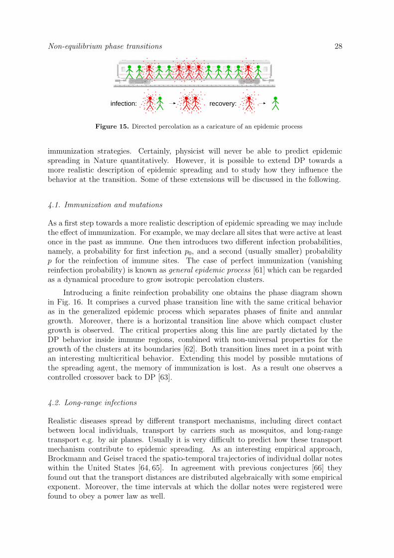
Directed percolation is often used as a caricatural process for epidemic spreading.Suppose that infected and healthy individuals are sitting in a train, as shown in Fig. 15.On the one hand, infected people infect their nearest neighbors with a certain probabilityper unit time. On the other hand, infected individuals may recover spontaneously.Depending on the rates for infection and recovery, this toy model for epidemic spreadingjust resembles a simple DP process.

Although DP is too simplistic to describe epidemic spreading in reality, there aresome important analogies. Certainly, epidemic spreading in Nature is a non-equilibriumprocess with a transition-like behavior at some threshold of the infection rate. Forexample, as an increasing number of people refuses vaccinations, the question arisesat which percentage of unprotected individuals certain diseases, that became almostextinct, will again percolate through the society.

Epidemic spreading in Nature is of course a much more complex phenomenon.For example, it takes place in a very disordered environment and involves short- andlong-range interactions. Moreover, individuals protect themselves by sophisticated


infection: recovery:

Figure 15. Directed percolation as a caricature of an epidemic process

immunization strategies. Certainly, physicist will never be able to predict epidemicspreading in Nature quantitatively. However, it is possible to extend DP towards amore realistic description of epidemic spreading and to study how they influence thebehavior at the transition. Some of these extensions will be discussed in the following.

4.1. Immunization and mutations

As a first step towards a more realistic description of epidemic spreading we may includethe effect of immunization. For example, we may declare all sites that were active at leastonce in the past as immune. One then introduces two different infection probabilities,namely, a probability for first infection p0, and a second (usually smaller) probabilityp for the reinfection of immune sites. The case of perfect immunization (vanishingreinfection probability) is known as general epidemic process [61] which can be regardedas a dynamical procedure to grow isotropic percolation clusters.

Introducing a finite reinfection probability one obtains the phase diagram shownin Fig. 16. It comprises a curved phase transition line with the same critical behavioras in the generalized epidemic process which separates phases of finite and annulargrowth. Moreover, there is a horizontal transition line above which compact clustergrowth is observed. The critical properties along this line are partly dictated by theDP behavior inside immune regions, combined with non-universal properties for thegrowth of the clusters at its boundaries [62]. Both transition lines meet in a point withan interesting multicritical behavior. Extending this model by possible mutations ofthe spreading agent, the memory of immunization is lost. As a result one observes acontrolled crossover back to DP [63].

4.2. Long-range infections

Realistic diseases spread by different transport mechanisms, including direct contactbetween local individuals, transport by carriers such as mosquitos, and long-rangetransport e.g. by air planes. Usually it is very difficult to predict how these transportmechanism contribute to epidemic spreading. As an interesting empirical approach,Brockmann and Geisel traced the spatio-temporal trajectories of individual dollar noteswithin the United States [64, 65]. In agreement with previous conjectures [66] theyfound out that the transport distances are distributed algebraically with some empiricalexponent. Moreover, the time intervals at which the dollar notes were registered werefound to obey a power law as well.


0 0,2 0,4 0,6 0,8 1

first infection probability p0

0

0,2

0,4

0,6

0,8

1

rein

fect

ion

prob

abili

ty p

compact growth

no growth

multicritical point

GEP

annular growth

Figure 16. Phase diagram for directed percolation with immunization (see text). The

right panel shows spreading by annular growth with fresh (green), active (red), and

immune (yellow) individuals.

Motivated by such empirical studies it is near at hand to generalize DP such thatthe spreading distances r are distributed as a power law

P (r) ∼ r−d−σ , (σ > 0) (41)

where σ is a control exponent. In the literature such algebraically distributed long-range displacements are known as Levy flights [67] and have been studied extensivelye.g. in the context of anomalous diffusion [68]. In the present context of epidemicspreading it turns out that such long-range flights do not destroy the transition, insteadthey change the critical behavior provided that σ is sufficiently small. More specifically,it was observed both numerically and in mean field approximations that the criticalexponents change continuously with σ [69–71]. As a major breakthrough, Janssen et al

introduced a renormalizable field theory for epidemic spreading transitions with spatialLevy flights [72], computing the critical exponents to one-loop order. Because of anadditional scaling relation only two of the three exponents were found to be independent.These results were confirmed numerically by Monte Carlo simulations [73].

4.3. Incubation times

As a second generalization one can introduce a similar long-range mechanism in temporal

direction. Such ‘temporal’ Levy flights may be interpreted as incubation times ∆tbetween catching and passing on the infection. As in the first case, these incubationtimes are assumed to be algebraically distributed as

P (∆t) ∼ ∆t−1−κ , (κ > 0) (42)

where κ is a control exponent. However, unlike spatial Levy flights, which take placeequally distributed in all directions, such temporal Levy flights have to be directedforward in time. Again it was possible to compute the exponents by a field-theoreticrenormalization group calculation [74].


0 0,5 1 1,5 2 2,5 3

σ

0

0,5

1

1,5

2

κ

DP

MF

dominated by spatial Levy flights

dominated bymixed phase incubation times

MFL

MFI

Figure 17. Phase diagram of DP with spatio-temporal Levy flights.

Recently, we studied the mixed case of epidemic spreading by spatial Levyflights combined with algebraically distributed incubation times [75]. In this case thecorresponding field theory was found to render two additional scaling relations, namely,

2β + (σ − d)ν⊥ − ν‖ = 0 , (43)

2β − dν⊥ + (κ− 1)ν‖ = 0 . (44)

Hence only one of the three exponents is independent. In particular, the dynamicalexponent z locks onto the ratio σ/κ. A systematic numerical and field-theoretic studyleads to a generic phase diagram in terms of the control exponents σ and κ which isshown in Fig. 17. It includes three types of mean-field phases, a DP phase, two phasescorresponding to purely spatial or purely temporal Levy flights, and a novel fluctuation-dominated phase describing the mixed case in which the critical exponents have beencomputed by a field-theoretic renormalization group calculation to one-loop order.

5. Surface growth and non-equilibrium wetting

Another interesting direction of non-equilibrium physics is the study of wetting far fromequilibrium. Wetting phenomena occur in a large variety of experiments, where a planarsubstrate is exposed to a gas phase. Usually the term ‘wetting’ refers to a situationwhere a bulk phase in contact with a substrate coexists with a layer of a different phasewhich is preferentially attracted to the surface of the substrate. By changing physicalparameters such as temperature and chemical potential, the system may undergo awetting transition from a non-wet phase, where the thickness of the layer stays finite,to a wet phase, where the layer becomes macroscopic.

In many experimental situations it is reasonable to assume that a wetting stationarylayer is in thermal equilibrium. In fact, methods of equilibrium statistical mechanicsturned out to be very successful in a large variety of theoretical and experimentalstudies [76]. Therefore, the question arises whether models for wetting far from


rate qrate q0

evaporation from themiddle of plateaus

evaporation at theedges of terraces

random deposition

rate p:rate 1:

��

��

��

��

��

��

��

��

��

��

��

��

Figure 18. Dynamical rules of the restricted solid-on-solid model for non-equilibrium

wetting. Neighboring heights are restricted to differ by at most one unit.

equilibrium may exhibit new physical phenomena which cannot be observed underequilibrium conditions.

Non-equilibrium wetting is usually modeled as a Kardar-Parisi-Zhang (KPZ)growth process [77] growing on top of a hard substrate. Theoretically such a system canbe described by a KPZ equation in a potential [78, 79]

∂h(x, t)

∂t= σ∇2h(x, t) − ∂V (h(x, t))

∂h(x, t)+ λ(∇h(x, t))2 + ξ(x, t) , (45)

where ξ(x, t) is a Gaussian noise. It is important to note that the nonlinear termλ(∇h(x, t))2 in this equation is a relevant perturbation of the underlying field theory, i.e.,even if λ is very small, it will be amplified under renormalization group transformations,driving the system away from thermal equilibrium. In fact, as can be shown byconstructing a closed loop, it is this term that breaks detailed balance.

Some time ago we introduced a simple solid-on-solid (SOS) model for non-equilibrium wetting in 1+1 dimensions [80–82]. The model is controlled by an adsorptionrate q, a desorption rate p, and optionally by a special deposition rate q0 on sites atheight zero (desorption at the edges takes place at rate 1, see Fig. 18). Setting q0 = qand varying the growth rate the model exhibits a continuous wetting transition at acertain critical growth rate qc(p). This wetting transition is related to the unpinningprocess of an interface from the substrate. Moreover, for q0 6= q the model can emulate ashort-range interaction between the interface and the substrate [83,84]. It was found thatsufficiently strong attractive interaction modifies the nature of the wetting transition andmakes it first order. In addition, it has been demonstrated that there exists an extendedregion in the phase diagram, where the pinned and the moving phases coexist in the sensethat the transition time from the pinned to the moving phase grows exponentially withthe system size so that the two phases become stable in the thermodynamic limit. Thistype of phase coexistence is in fact a new phenomenon that occurs only far away fromequilibrium and should be experimentally observable.

6. Summary

At the end of this lecture let us address the crucial question to what extent theserecent developments in the field of non-equilibrium statistical physics can be confirmedexperimentally. Unfortunately, the experimental evidence is still very poor. Forexample, although many transition-like phenomena far from equilibrium can be seen


0.0 0.5 1.0 1.5 2.0p

0.0

0.5

1.0

1.5

q

phase coexistencepinned

moving

Figure 19. Phase diagram of the solid-on-solid model for non-equilibrium wetting.

The bold black line represents the second-order phase transition line. For sufficiently

small q0 the transition becomes first order and a region emerges (striped in the figure),

where the pinned and the moving phase coexist.

in Nature, there is so far no experiment in which the exponents of DP or any other classof absorbing phase transitions can be reproduced quantitatively in a reliable way. Thisis surprising since various possible experimental realizations have been proposed [85].For deposition-evaporation phenomena the situation is not much better: Up to now noconvincing experiment is known in which the exponents of the KPZ universality classcan be confirmed.

The poor experimental evidence could be partly due to the fact that manyexperimentalists are not yet fully aware of recent developments in non-equilibriumstatistical physics. Similarly, many theoretical physicists do not care so much aboutexperiments and regard instead the computer as the beauty of Nature. However, thepoor experimental evidence could have more fundamental reasons. For example, despitethe robustness and simplicity of DP, the existence of an absorbing state is a highlyidealized requirement that is difficult to realize experimentally.

With the advent of modern nanotechnology, however, the situation could change innear future. Therefore, it is particularly important to understand the crossover betweenquantum and classical behavior in order to find out where the models of non-equilibriumstatistical physics can be applied. All in all we should be optimistic: Universality classeswhich are as fundamental as DP or KPZ are so beautiful that they should be relevantin Nature. In fact, in equilibrium statistical mechanics there was quite a long wayfrom Onsagers solution of the two-dimensional Ising model to the ample experimentalevidence that is available today.

References

[1] E. Joos, H. D. Zeh, C. Kiefer, D. Giulini, J. Kupsch, and I.-O. Stamatescu, Decoherence and the

appearance of a classical world in quantum theory, Springer, Berlin, 2003.

[2] T. M. Liggett, Interacting particle systems, Springer, Berlin, 1985.

[3] H. Spohn, Large scale dynamics of interacting particles, Springer, Berlin, 1991.

[4] A. M. Polyakov, Conformal symmetry of critical fluctuations, Sov. Phys. JETP Lett. 12, 381

(1970).

[5] J. L. Cardy, Conformal Invariance, in Phase transitions and critical phenomena, edited by


C. Domb and J. L. Lebowitz, volume 11, Academic Press, New York, 1987.

[6] M. Henkel, Conformal Invariance and Critical Phenomena, Springer Verlag, Berlin, 1999.

[7] A. L. Barabasi and H. Stanley, Fractal concepts in surface growth, Cambridge University Press,

U.K., 1995.

[8] D. E. Wolf, M. Schreckenberg, and A. Bachem, Traffic and granular flow, World Scientific,

Singapore, 1996.

[9] W. Kinzel, Percolation structures and processes, in Ann. Isr. Phys. Soc., edited by G. Deutscher,

R. Zallen, and J. Adler, volume 5, Adam Hilger, Bristol, 1983.

[10] J. Marro and R. Dickman, Nonequilibrium phase transitions in lattice models, Cambridge

University Press, Cambridge, 1999.

[11] P. Grassberger, Directed percolation: results and open problems, in Nonlinearities in complex

systems, proceedings of the 1995 Shimla conference on complex systems, edited by S. Puri et al.,

Narosa Publishing, New Dehli, 1997.

[12] G. Odor, Universality classes in nonequilibrium lattice systems, Rev. Mod. Phys. 76, 663–724

(2004).

[13] S. Lubeck, Universal scaling behavior of non-equilibrium phase transitions, Int. J. Mod. Phys.

18, 3977–4118 (2004).

[14] H. Hinrichsen, Non-equilibrium critical phenomena and phase transitions into absorbing states,

Adv. Phys. 49, 815–958 (2000).

[15] D. Stauffer and A. Aharony, Introduction to Percolation Theory, Taylor & Francis, London, 1992.

[16] I. Jensen, Low-density series expansions for directed percolation: III. Some two-dimensional

lattices, J. Phys. A 37, 6899–6915 (2004).

[17] E. Domany and W. Kinzel, Equivalence of cellular automata to Ising models and directed

percolation, Phys. Rev. Lett. 53, 311–314 (1984).

[18] W. Kinzel, Phase transitions of cellular automata, Z. Phys. B 58, 229–244 (1985).

[19] S. Wolfram, Statistical mechanics of cellular automata, Rev. Mod. Phys. 55, 601–644 (1983).

[20] G. F. Zebende and T. J. P. Penna, The Domany-Kinzel cellular automaton phase diagram, J.

Stat. Phys. 74, 1273–1279 (1994).

[21] I. Dornic, H. Chate, J. Chave, and H. Hinrichsen, Critical coarsening without surface tension: the

voter universality class, Phys. Rev. Lett. 87, 5701–5704 (2001).

[22] T. E. Harris, Contact interactions on a lattice, Ann. Prob. 2, 969 (1974).

[23] R. Dickman and J. K. da Silva, Moment ratios for absorbing-state phase transitions, Phys. Rev.

E 58, 4266–4270 (1998).

[24] J. F. F. Mendes, R. Dickman, M. Henkel, and M. C. Marques, Generalized scaling for models

with multiple absorbing states, J. Phys. A 27, 3019–3028 (1994).

[25] H. K. Janssen, On the nonequilibrium phase transition in reaction-diffusion systems with an

absorbing stationary state, Z. Phys. B 42, 151–154 (1981).

[26] P. Grassberger, On phase transitions in Schlogl’s second model, Z. Phys. B 47, 365–374 (1982).

[27] H. K. Janssen and U. C. Tauber, The field theory approach to percolation processes, Ann. Phys.

(N.Y.) 315, 147–192 (2005).

[28] U. C. Tauber, M. J. Howard, and B. P. Vollmayr-Lee, Applications of field-theoretic

renormalization group methods to reaction-diffusion problems, J. Phys. A 38, R79–R131 (2005).

[29] R. Rammal, C. Tannous, and P. Brenton, Flicker (1/f) noise in percolation networks: A new

hierarchy of exponents, Phys. Rev. Lett. 54, 1718–1721 (1985).

[30] L. de Arcangelis, S. Redner, and A. Coniglio, Anomalous voltage distribution of random resistor

networks and a new model for the backbone at the percolation threshold, Phys. Rev. B 31,

4725–4727 (1985).

[31] O. Stenull and H. K. Janssen, Transport on directed percolation clusters, Phys. Rev. E 63,

025103 (2001).

[32] H. Hinrichsen, O. Stenull, and H. K. Janssen, Multifractal current distribution in random-diode

networks, Phys. Rev. E 65, 045104–045107 (2002).


[33] C. N. Yang and T. D. Lee, Statistical theory of equations of state and phase transitions: 1. Theory

of condensation, Phys. Rev. E 87, 404–409 (1952).

[34] C. N. Yang and T. D. Lee, Statistical theory of equations of state and phase transitions: 2. Lattice

gas and Ising model, Phys. Rev. E 87, 420–419 (1952).

[35] B. Derrida, L. de Seeze, and C. Itzykson, Fractal structure of zeros in hierarchical models, J.

Stat. Phys. 33, 559–569 (1983).

[36] P. F. Arndt, Yang-Lee theory for a nonequilibrium phase transition, Phys. Rev. Lett. 84, 814–817

(2000).

[37] S. M. Dammer, S. R. Dahmen, and H. Hinrichsen, Yang-Lee zeros for a nonequilibrium phase

transition, J. Phys. A 35, 4527–4539 (2002).

[38] D. Zhong and D. ben Avraham, Universality class of two-offspring branching annihilating random

walks, Phys. Lett. A 209, 333–337 (1995).

[39] J. Cardy and U. C. Tauber, Theory of branching and annihilating random walks, Phys. Rev.

Lett. 77, 4780 (1996).

[40] J. Cardy and U. C. Tauber, Field theory of branching and annihilating random walks, J. Stat.

Phys. 90, 1–56 (1998).

[41] J. T. Cox and D. Griffeath, Diffusive clustering in the two-dimensional voter model, Annals of

Probability 14, 347–370 (1986).

[42] M. Scheucher and H. Spohn, A soluble kinetic model for spinodal decomposition, J. Stat. Phys.

53, 279–294 (1988).

[43] L. Frachebourg and P. L. Krapivsky, Exact results for kinetics of catalytic reactions, Phys. Rev.

E 53, R3009–R3012 (1996).

[44] O. A. Hammal, H. Chate, I. Dornic, and M. A. Munoz, Langevin description of critical phenomena

with two symmetric absorbing states, Phys. Rev. Lett. 94, 230601–230604 (2005).

[45] M. Rossi, R. Pastor-Satorras, and A. Vespignani, Universality class of absorbing phase transitions

with a conserved field, Phys. Rev. Lett. 85, 1803–1806 (2000).

[46] S. S. Manna, Two-state model of self-organized criticality, J. Phys. A 24, L363 (1991).

[47] M. Henkel and H. Hinrichsen, The non-equilibrium phase transition of the pair-contact process

with diffusion, J. Phys. A 37, R117–R159 (2004).

[48] P. Grassberger, On phase transitions in Schlog’s second model, 47, 365 (1982).

[49] M. J. Howard and U. C. Tauber, ‘Real’ versus ‘imaginary’ noise in diffusion-limited reactions, J.

Phys. A 30, 7721 (1997).

[50] E. Carlon, M. Henkel, and U. Schollwock, Critical properties of the reaction-diffusion model

2A → 3A, 2A → ∅, Phys. Rev. E 63, 036101 (2001).

[51] J. Kockelkoren and H. Chate, Absorbing phase transition of branching-annihilating random walks,

Phys. Rev. Lett. 90, 125701 (2003).

[52] G. Odor, Critical behaviour of the one-dimensional annihilation-fission process 2A → ∅, 2A → 3A,

Phys. Rev. E 62, R3027 (2000).

[53] G. Odor, Critical behaviour of the one-dimensional diffusive pair-contact process, Phys. Rev. E

67, 016111 (2003).

[54] M. Paessens and G. M. Schutz, Phase transitions and correlations in the bosonic pair contact

process with diffusion: exact results, J. Phys. A 37, 4709–4722 (2004).

[55] H. Hinrichsen, Cyclically coupled spreading and pair-annihilation, 291, 275 (2001).

[56] J. D. Noh and H. Park, Novel universality class of absorbing transitions with continuously varying

exponents, Phys. Rev. E 69, 016122 (2004).

[57] R. Dickman and M. A. F. de Menezes, Nonuniversality in the pair-contact process with diffusion,

Phys. Rev. E 66, 045101 (2002).

[58] H. Hinrichsen, Stochastic cellular automaton for the coagulation-fission process 2A → 3A,

2A → A, 320, 249 (2003).

[59] G. T. Barkema and E. Carlon, Universality in the pair-contact process with diffusion, Phys. Rev.

E 68, 036113 (2003).


[60] H. Hinrichsen, The diffusive pair-contact process and non-equilibrium wetting, 2003, unpublished

notes, cond-mat/0302381.

[61] J. L. Cardy and P. Grassberger, Epidemic models and percolation, J. Phys. A 18, L267–L271

(1985).

[62] A. Jimenez-Dalmaroni and H. Hinrichsen, Epidemic spreading with immunization, Phys. Rev. E

68, 036103–036114 (2003).

[63] S. M. Dammer and H. Hinrichsen, Epidemic spreading with immunization and mutations, Phys.

Rev. E 68, 016114–016121 (2003).

[64] L. Hufnagel, D. Brockmann, and T. Geisel, Forecast and control of epidemics in a globalized

world, Proc. Nat. Acam. Sci. 101, 15124–15129 (2004).

[65] D. Brockmann, L. Hufnagel, and T. Geisel, Human dispersal on geographical scales, 2005,

preprint, submitted.

[66] D. Mollison, Spatial contact models for ecological and epidemic spread, J. Roy. Stat. Soc. B 39,

283 (1977).

[67] J.-P. Bouchaud and A. Georges, Anomalous diffusion in disordered media: statistical mechanics,

models and physical applications, Phys. Rep. 195, 127–293 (1990).

[68] H. C. Fogedby, Langevin equations for continuous Levy flights, Phys. Rev. E 50, 1657–1660

(1994).

[69] P. Grassberger, in Fractals in physics, edited by L. Pietronero and E. Tosatti, Elsevier, Amsterdam,

1986.

[70] M. C. Marques and A. L. Ferreira, Critical behaviour of a long-range non-equilibrium system, J.

Phys. A 27, 3389–3395 (19).

[71] E. V. Albano, Branching annihilating Levy flights: Irreversible phase transitions with long-range

interactions, Europhys. Lett. 34, 97–102 (1996).

[72] H. K. Janssen, K. Oerding, F. van Wijland, and H. J. Hilhorst, Levy-flight spreading of epidemic

processes leading to percolating clusters, Euro. Phys. J. B 7, 137–145 (1999).

[73] H. Hinrichsen and M. Howard, A model for anomalous directed percolation, Euro. Phys. J. B 7,

635–643 (1999).

[74] A. Jimenez-Dalmaroni and J. Cardy, 2005, in preparation.

[75] J. Adamek, M. Keller, A. Senftleben, and H. Hinrichsen, Epidemic spreading with long-range

infections and incubation times, J. Stat. Mech. , to appear (2005).

[76] S. Dietrich, Wetting phenomena, in Phase transitions and critical phenomena, edited by C. Domb

and J. L. Lebowitz, volume 12, Academic Press, London, 1988.

[77] G. P. M. Kardar and Y.-C. Zhang, Dynamic scaling of growing interfaces, Phys. Rev. Lett. 56,

889–892 (1986).

[78] Y. Tu, G. Grinstein, and M. A. Munoz, Systems with multiplicative noise: critical behavior from

KPZ equation and numerics, Phys. Rev. Lett. 78, 274–277 (1997).

[79] M. A. Munoz and T. Hwa, On nonlinear diffusion with multiplicative noise, Europhys. Lett. 41,

147–152 (1998).

[80] U. Alon, M. R. Evans, H. Hinrichsen, and D. Mukamel, Roughening transition in a one-dimensional

growth process, Phys. Rev. Lett. 76, 2746–2749 (1996).

[81] U. Alon, M. Evans, H. Hinrichsen, and D. Mukamel, Smooth phases, roughening transitions, and

novel exponents in one-dimensional growth models, Phys. Rev. E 57, 4997–5012 (1998).

[82] H. Hinrichsen, R. Livi, D. Mukamel, and A. Politi, A model for nonequilibrium wetting transitions

in two dimensions, Phys. Rev. Lett. 79, 2710–2713 (1997).

[83] H. Hinrichsen, R. Livi, D. Mukamel, and A. Politi, First order phase transition in a 1+1-

dimensional nonequilibrium wetting process, Phys. Rev. E 61, R1032–R1035 (2000).

[84] H. Hinrichsen, R. Livi, D. Mukamel, and A. Politi, Wetting under non-equilibrium conditions,

Phys. Rev. E 68, 041606 (2003).

[85] H. Hinrichsen, On possible experimental realizations of directed percolation, Braz. J. Phys. 30,

69–82 (2000).

non-equilibrium phase transitions -...

Documents