JOURNAL OF ECONOMIC THEORY 43, 355-363 (1987)

Non-connectedness of the Set of Equilibrium Money Prices: The Overlapping-Generations Economy

JAMES PECK *

J. L. Kellogg Graduate School of Management, Northwestern University, Evanston, Illinois 60201

Received December 12, 1984; revised August 31, 1986

Consider the overlapping-generations economy with nominal taxes and transfers. Under some conditions, the set of equilibrium money prices is a non-negative inter- val. It has not been known whether this set can consist of two or more disjoint intervals. Three examples are provided here in which the set of equilibrium money prices is a non-connected set. The examples are for a finite-horizon balanced economy, an infinite-horizon balanced economy, and an infinite-horizon non-balan- ced economy. Journal of Economic Literature Classitication Numbers: 021,023. tc:’ 1987 Academic Press, Inc.

Overlapping-generations models with money typically exhibit a mul- tiplicity of equilibria in which the equilibrium price of money takes on a range of values. Balasko and Shell [3] find that for finite-horizon economies with a balanced’ tax-transfer policy, the set of equilibrium money prices contains an interval [0, pm], where p”’ is a positive scalar. If the tax-transfer policy is not balanced, the price of money must be zero.2 For infinite-horizon economies with a strongly balanced3 tax-transfer

*Support from the National Science Foundation under Grant SES-8348450 is acknowledged. I would also like to thank Karl Shell for his advice and encouragement. All remaining errors are my own.

’ The tax-transfer policy r = (~a, r,, . . . . rT) is said to be balanced if we have x:i, r, = 0. That is, a tax-transfer policy is balanced if the out-standing government debt is zero on the terminal date. See [3, Definition 3.11.

‘This follows immediately from Walras’ Law (see 13. Proposition 3.21). The intuition is that all consumers are on their budget lines, so the value of aggregate excess demand equals the value of the money supply. In equilibrium, excess demand equals zero, so the value of the money supply is zero. Either the money supply is zero, and the tax-transfer policy is balanced, or the price of money is zero.

3 The tax-transfer policy T = (~a, r,, ..,, T,, . ..) E Iw e is said to be strongly balanced if there is an integer t’ with the property xiZ0 rJ = 0 for I 2 I’.

355 0022-0531/87 $3.00

Copyright :I: 1987 by Academic Press. Inc. All rights of reproduction m any form reserved.

356 JAMES PECK

policy, the set of equilibrium money prices contains a proper interval; however, there may even be a range of money prices when the policy is not strongly balanced. Balasko and Shell suggest that there are examples where the set of equilibrium money prices contains a proper interval, but where the entire set consists of two unconnected intervals or some more com- plicated structure. I present three examples, satisfying all the regularity assumptions of [3], in which the set of equilibrium money prices is not connected.

Each consumer is assumed to have preferences giving rise to a utility function that is strictly monotonic, differentiable, strictly quasi-concave, and with the closure of each indifference surface contained in the strictly positive orthant (see Balasko and Shell [ 1, p. 1151). It is further assumed that consumers, for the periods in which they are alive, have strictly positive endowments. I follow the notation of Balasko and Shell [3].

EXAMPLE 1 (finite economy, balanced tax-transfer policy). Let there be one commodity per period, I= 1, and a finite time horizon of length T. There is one consumer, Mr. 0, alive at the beginning of economic time who lives only through period 1. All other consumers are born in period t (t= 1, 2, 3, . . . . T- 1) and live in periods t and t + 1. There is one consumer born in each period except period 2, in which two consumers are born (call them Mr. 2A and Mr. 2B)4. Index the consumers by their birthdates h = 0, 1, 2A, 2B, 3, . . . . T- 1.

For this economy, endowments are given by

w,=o:,=4,

WI = (co:, co:, = (14,4),

0 - (O:A, 2A - w:A) = (4, 16),

w - (49 2B - w&) = (4, 16),

and wh=(o;,o;+1)=(4,4) for h = 3, 4, . . . . T- 1.

The tax-transfer policy, r = (r,,, r,, tZA, rZB, t3, r4, . . . . rT- r) E RT+‘, where the scalar rh is positive for a tax on consumer h and negative for a transfer to consumer h, is given by

4 It should be noted that Balasko and Shell assume exactly one consumer is born in each period, but the assumption is not meant to be restrictive. This example is completely in the spirit of [3].

MONEY PRICES 357

To = - 10,

5, = 10,

T = 2.4 50,

T - - 2B 0,

T3= -50,

and

T,=o for h=4, 5, . . . . T- 1.’

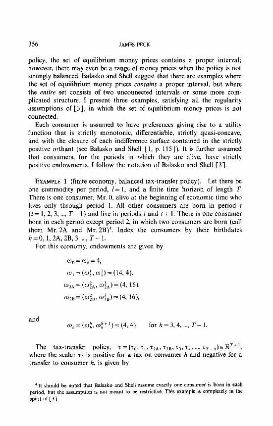
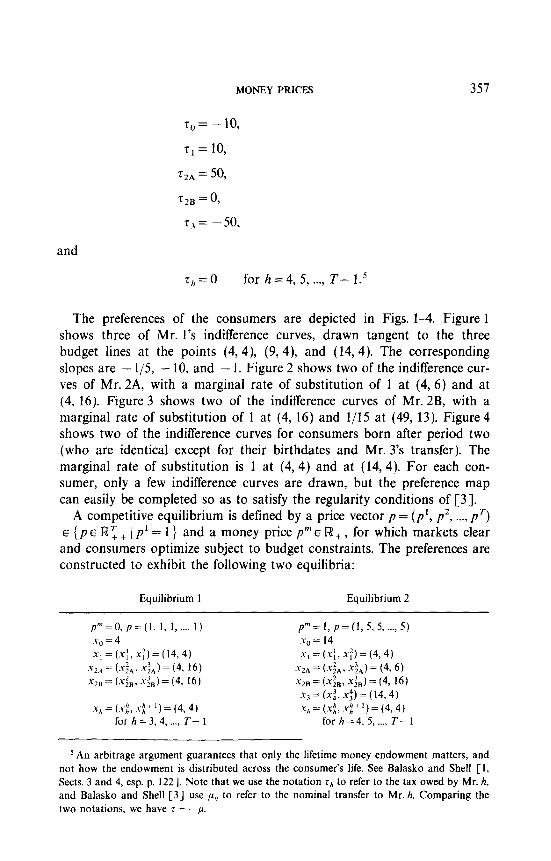
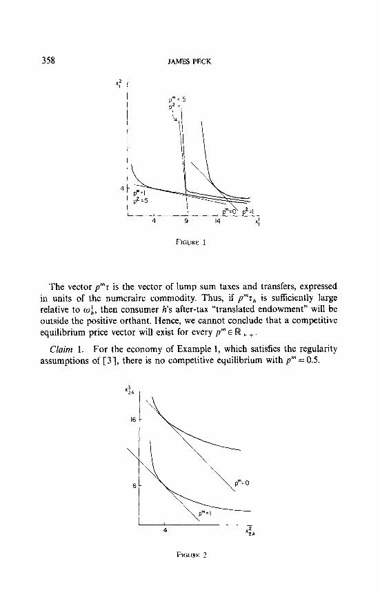
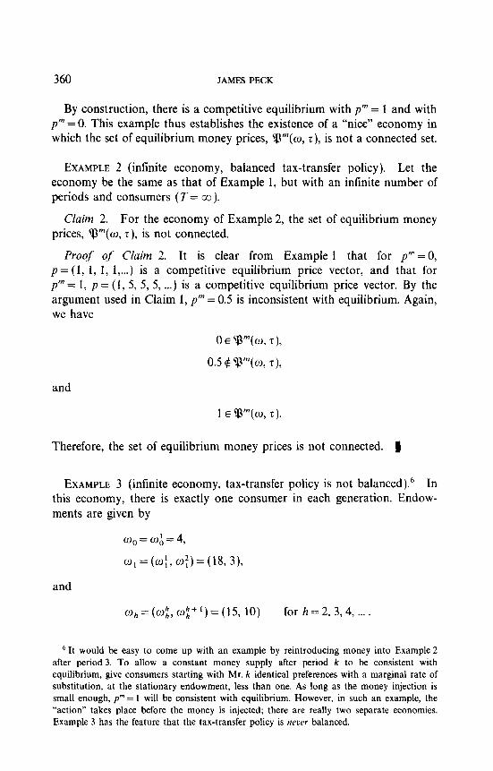
The preferences of the consumers are depicted in Figs. 1-4. Figure 1 shows three of Mr. l’s indifference curves, drawn tangent to the three budget lines at the points (4,4), (9,4), and (14,4). The corresponding slopes are - l/5, - 10, and - 1. Figure 2 shows two of the indifference cur- ves of Mr. 2A, with a marginal rate of substitution of 1 at (4, 6) and at (4, 16). Figure 3 shows two of the indifference curves of Mr. 2B, with a marginal rate of substitution of 1 at (4, 16) and l/15 at (49, 13). Figure 4 shows two of the indifference curves for consumers born after period two (who are identical except for their birthdates and Mr. 3’s transfer). The marginal rate of substitution is 1 at (4,4) and at (14,4). For each con- sumer, only a few indifference curves are drawn, but the preference map can easily be completed so as to satisfy the regularity conditions of [3].

A competitive equilibrium is defined by a price vector p = (p’, p2, . . . . p’) E (p E lRT + ( p’ = 1) and a money price p” E R! + , for which markets clear and consumers optimize subject to budget constraints. The preferences are constructed to exhibit the following two equilibria:

Equilibrium 1 Equilibrium 2

p”=O,p=(l, 1, I,..., 1) x0 = 4 x, = (x-f, x:, = (14.4)

5 2.4 = (xi,, x:,,= (4. 16) xzB = (x;,. x;,) = (4. 16)

x,=(x;,x;+l)=(4,4) for h = 3, 4, . . . . T- 1

p”=l,p=(l, 5, 5, . ..) 5) x-g = 14 5, = (xf, x;, = (4,4)

x2,, = (.Y&. .&) = (4, 6) xzB = (x;,, &) = (4, 16)

I) = (xi, x;, = (14,4) .Yh=(.Y~,x:+‘)=(4,4)

for h = 4, 5, _.., T- 1

5 An arbitrage argument guarantees that only the lifetime money endowment matters, and not how the endowment is distributed across the consumer’s life. See Balasko and Shell [l, Sects. 3 and 4, esp. p. 1221. Note that we use the notation rb to refer to the tax owed by Mr. h, and Balasko and Shell [3] use p,, to refer to the nominal transfer to Mr. h. Comparing the two notations, we have 7 = -p.

358 JAMES PECK

FIGURE 1

The vector p”z is the vector of lump sum taxes and transfers, expressed in units of the numeraire commodity. Thus, if pm~,, is sufiiciently large relative to oj,, then consumer h’s after-tax “translated endowment” will be outside the positive orthant. Hence, we cannot conclude that a competitive equilibrium price vector will exist for every p” E IR + +

Claim 1. For the economy of Example 1, which satisfies the regularity assumptions of [3], there is no competitive equilibrium with pm = 0.5.

FIGURE 2

MONEY PRICES 359

16 -

PZ 1 _I_ p3 15

I 4 49 x&

FIGURE 3

Proof of Claim 1. When pm = 0.5 we have x,, = 9. Market clearing in period 1 implies that we have xi = 9, and for Mr. 1 to be on his budget line we must have xi = (9,4). However, for (9,4) to maximize Mr. l’s utility, the marginal rate of substitution at that point, which is 10, must equal the price ratio p’/p2. It follows that p2=0.1 must hold to be consistent with equilibrium. Whenever p3 < 24.6/16 occurs, the wealth of Mr. 2A is negative, which is inconsistent with equilibrium. Whenever we have p3 2 24.6/16, Mr. 2B demands more than the economy’s total resource of commodity 2, x& > 12. Obviously, market clearing fails to hold and there is no competitive equilibrium. We have contradicted the hypothesis that pm = 0.5 is consistent with competitive equilibrium. 1

& pm=0 pm=1

4 14 x3 3

FIGURE 4

360 JAMES PECK

By construction, there is a competitive equilibrium with pm = 1 and with p”=O. This example thus establishes the existence of a “nice” economy in which the set of equilibrium money prices, ‘$“(o, t), is not a connected set.

EXAMPLE 2 (infinite economy, balanced tax-transfer policy). Let the economy be the same as that of Example 1, but with an infinite number of periods and consumers (T= cc ).

Claim 2. For the economy of Example 2, the set of equilibrium money prices, Cpm(w, z), is not connected.

Proof of Claim 2. It is clear from Example 1 that for p” = 0, p = (1, 1, 1, l,...) is a competitive equilibrium price vector, and that for pm = 1, p = (1, 5, 5, 5, . ..) is a competitive equilibrium price vector. By the argument used in Claim 1, pm = 0.5 is inconsistent with equilibrium. Again, we have

and

0 E V”(o, z),

0.5 & ‘p”(G z),

1 E cp”(0, T).

Therefore, the set of equilibrium money prices is not connected. 1

EXAMPLE 3 (infinite economy, tax-transfer policy is not balanced).6 In this economy, there is exactly one consumer in each generation. Endow- ments are given by

0,=0:,=4,

w,=(w:,w:)=(18,3),

and

oh=(o;,o;+‘)=(15, 10) for h = 2, 3,4, . . . .

‘It would be easy to come up with an example by reintroducing money into Example 2 after period 3. To allow a constant money supply after period k to be consistent with equilibrium, give consumers starting with Mr. k identical preferences with a marginal rate of substitution, at the stationary endowment, less than one. As long as the money injection is small enough, pm = 1 will be consistent with equilibrium. However, in such an example, the “action” takes place before the money is injected; there are really two separate economies. Example 3 has the feature that the tax-transfer policy is never balanced.

MONEY PRICES 361

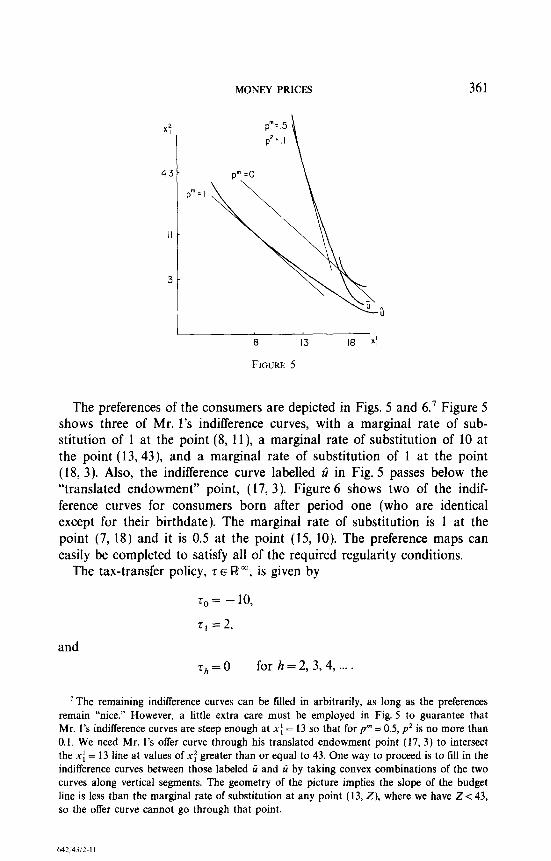
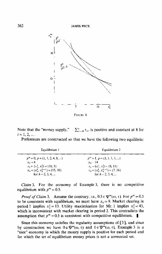
The preferences of the consumers are depicted in Figs. 5 and 6.’ Figure 5 shows three of Mr. l’s indifference curves, with a marginal rate of sub- stitution of 1 at the point (8, 1 l), a marginal rate of substitution of 10 at the point (13,43), and a marginal rate of substitution of 1 at the point (18, 3). Also, the indifference curve labelled li in Fig. 5 passes below the “translated endowment” point, (17,3). Figure 6 shows two of the indif- ference curves for consumers born after period one (who are identical except for their birthdate). The marginal rate of substitution is 1 at the point (7, 18) and it is 0.5 at the point (15, 10). The preference maps can easily be completed to satisfy all of the required regularity conditions.

The tax-transfer policy, 7 E R”, is given by

and

To= -10,

t, =2,

z,=o for h = 2, 3, 4, . . . .

‘The remaining indifference curves can be filled in arbitrarily, as long as the preferences remain “nice.” However, a little extra care must be employed in Fig. 5 to guarantee that Mr. l’s indifference curves are steep enough at xi = 13 so that for pm = 0.5, p2 is no more than 0.1. We need Mr. l’s offer curve through his translated endowment point (17, 3) to intersect the .x-i = 13 line at values of x: greater than or equal to 43. One way to proceed is to till in the indifference curves between those labeled ri and ti by taking convex combinations of the two curves along vertical segments. The geometry of the picture implies the slope of the budget line is less than the marginal rate of substitution at any point (13, Z), where we have Z < 43, so the offer curve cannot go through that point.

642:43/?-I I

362 JAMES PECK

7 15 Xnh

FIGURE 6

Note that the “money supply,” - 1: = 0 r,, is positive and constant at 8 for t = 1, 2, . . . .

Preferences are constructed so that we have the following two equilibria:

Equilibrium 1 Equilibrium 2

p”=O,p=(l,1,2,4,8 ,...) x,=4 xl= (.x;, x;,= (18, 3) Xh=(X:,X;+‘)=(15, 10)

for h = 2, 3. 4,

pm= 1, p=(l, 1, I, 1, . ..) x0 = 14 .r,=(x;,.r;)=(S, 11) l*=(x~,.Y~+‘)=(7,18)

for h = 2, 3,4,

Claim 3. For the economy of Example 3, there is no competitive equilibrium with pm = 0.5.

Proof of Claim 3. Assume the contrary, i.e., 0.5 E ‘p”(w, r). For pm = 0.5 to be consistent with equilibrium, we must have x,, = 9. Market clearing in period 1 implies xi = 13. Utility maximization for Mr. 1 implies xf = 43, which is inconsistent with market clearing in period 2. This contradicts the assumption that p” = 0.5 is consistent with competitive equilibrium. g

Since this economy satisfies the regularity assumptions of [3], and since by construction we have OE ‘+Q”‘(w, r) and 1 E ‘p”(o, r), Example 3 is a “nice” economy in which the money supply is positive for each period and for which the set of equilibrium money prices is not a connected set.

MONEY PRICES 363

CONCLUDING REMARKS

I have presented examples in which the set of equilibrium money prices is not connected for each of three types of overlapping-generations economies. Example 1 is based on a finite time-horizon economy and hence an economy with a balanced tax-transfer policy. Example 2 is based on an infinite time-horizon economy and a strongly balanced tax-transfer policy. Example 3 is also based on an economy with an infinite time-horizon, but the tax-transfer policy is not balanced in any sense; the public debt (here the money supply as well) is constant.

These examples might seem to be restrictive, but this is not the case. In Examples 1 and 2, Mr. 2A and Mr. 2B have equal marginal rates of sub- stitution at their endowments. Mr. 2A faces the same budget set under the pm = 0 and pm = 1 equilibria. These features are imposed to simplify the calculation of equilibrium trades and to keep Figs. l-4 as uncluttered as possible. They are by no means essential to the result. In Example 3, when pm = 1, the economy eventually finds itself in a steady state. As long as Mr. 2’s offer curve crosses the X: = 7 line below xi = 18, pm = 1 is consistent with equilibrium and the result still holds.

What drives the result for these three examples is the nature of Mr. l’s preferences. The marginal rate of substitution is extremely high in a region of Mr. l’s preference map, which causes p” =OS to be inconsistent with equilibrium. The region of high marginal rates of substitution does not come into play when pm = 0 and p” = 1, so those money prices are consistent with equilibrium. These examples of a non-connected set of equilibrium money prices rely on strong income effects, but there is certainly nothing pathological about strong income effects.

REFERENCES

1. Y. BALASKO AND K. SHELL, The overlapping-generations model II. The case of pure exchange with money, J. Econ. Theory 24 (1981), 112-142.

2. Y. BALASKO AND K. SHELL, “Lump-Sum Taxes and Transfers: The Overlapping Generations Model with Money,” CARESS Working Paper No. 8346R, University of Pennsylvania, 1983.

3. Y. BALASKO AND K. SHELL, Lump-sum taxes and transfers: Public debt in the overlapping- generations model, in “Essays in Honor of Kenneth J. Arrow, Vol. II: Equilibrium Analysis” (W. Heller, R. Starr, and D. Starrett, Eds.) Chap. 5, pp. 121-153, Cambridge Univ. Press, 1986.

4. Y. BALASKO AND K. SHELL, On taxation and competitive equilibrium, in “Optimalite et structures: Melanges en hommage a Edouard Rossier” (G. Ritschard and D. Royer, Eds.) pp. 69-83, Economica, Paris, 1985.