U. S. DEPARTMENT OF COMMERCENational Oceanic and Atmospheric AdministrationNational Marine Fisheries ServiceSouthwest Fisheries Science Center

NOAA-TM-NMFS-SWFSC-525

FEBRUARY 2014

NOAA Technical Memorandum NMFS

Michael S. Mohr

Michael R. O’Farrell

Fisheries Ecology DivisionSouthwest Fisheries Science Center

National Marine Fisheries Service, NOAA110 Shaffer Road

Santa Cruz, CA 95060, USA

THE SACRAMENTO HARVEST MODEL (SHM )

The National Oceanic and Atmospheric Administration (NOAA), organized in

1970, has evolved into an agency that establishes national policies and manages

and conserves our oceanic, coastal, and atmospheric resources. An

organizational element within NOAA, the Office of Fisheries, is responsible for

fisheries policy and the direction of the National Marine Fisheries Service (NMFS).

In addition to its formal publications, the NMFS uses the NOAA Technical

Memorandum series to issue informal scientific and technical publications when

complete formal review and editorial processing are not appropriate or feasible.

Documents within this series, however, reflect sound professional work and may

be referenced in the formal scientific and technical literature.

MOSTA PHD EN RA ICCI AN DA ME IC N

O ISL TA RN ATOI IOT

A

U

E

.S

C.

RD

EEMPA MR OT CM FEN O

MOSTA PHD ENA ICCI AN DA ME IC NISL TA RN A

TOI IOTA N

N

U

E

.S

C.

RD

EEMPA MR OCM FENT O

NOAA Technical Memorandum NMFSThis TM series is used for documentation and timely communication of preliminary results, interim reports, or specialpurpose information. The TMs have not received complete formal review, editorial control, or detailed editing.

NOAA Technical Memorandum NMFSThis TM series is used for documentation and timely communication of preliminary results, interim reports, or specialpurpose information. The TMs have not received complete formal review, editorial control, or detailed editing.

NOAA-TM-NMFS-SWFSC-525

National Oceanic and Atmospheric Administration

U.S. DEPARTMENT OF COMMERCE

National Oceanic and Atmospheric AdministrationPenny S. Pritzker, Secretary of Commerce

Dr. Kathryn D. Sullivan, Acting AdministratorDr. Kathryn D. Sullivan, Acting AdministratorNational Marine Fisheries ServiceNational Marine Fisheries ServiceEileen Sobeck, Assistant Administrator for Fisheries

FEBRUARY 2014

Michael S. Mohr

Michael R. O’Farrell

Fisheries Ecology DivisionSouthwest Fisheries Science Center

National Marine Fisheries Service, NOAA110 Shaffer Road

Santa Cruz, CA 95060, USA

THE SACRAMENTO HARVEST MODEL (SHM )

 

Abstract

Sacramento River fall Chinook (SRFC) salmon contribute heavily to California and Oregon ocean

salmon fisheries and support a Sacramento basin recreational river fishery. An overhaul of the

SRFC stock assessment methods commenced in 2008, including development of a new ocean abun-

dance index (the Sacramento Index: SI) and harvest model (the Sacramento Harvest Model: SHM),

both of which are currently used for assessment and fishery planning within the annual Pacific Fish-

ery Management Council (PFMC) salmon management process. The SHM is an aggregate-age

harvest model that, when combined with the forecast SI, predicts the SRFC spawner escapement

and overall exploitation rate given proposed ocean and river fishery management measures. This

memorandum provides comprehensive documentation of the SHM, beginning with a description

of the basic model structure. Detailed descriptions of the SHM ocean and river submodels, and

the methods used to estimate their parameters follow. The SHM has been a central part of PFMC

salmon fishery planning since its initial development and will likely remain an important part of

that process until improved coded-wire tag and escapement data sets for this stock mature, poten-

tially enabling an age-structured assessment.

1

1 Introduction

Sacramento River fall Chinook (SRFC) salmon are the largest contributor to ocean salmon fishery

harvest off the coasts of California and Oregon (O’Farrell et al. 2013). Management of salmon

fisheries through the Pacific Fishery Management Council (PFMC) aims to meet, in expectation,

the annual conservation objectives for all salmon stocks, including SRFC. In the case of SRFC, the

conservation objective is a spawning escapement of 122,000–180,000 natural and hatchery adults

(≥ age-3). Since the adoption of Amendment 16 to the Pacific Coast Salmon Fishery Management

Plan (PFMC 2012), SRFC have been managed according to a harvest “control rule”, depicted in

Figure 1, that specifies the maximum allowable overall exploitation rate on SRFC as a function of

the Sacramento Index (SI), an index of adult SRFC ocean abundance (O’Farrell et al. 2013). Here,

the overall exploitation rate is defined as the sum of SRFC adult ocean and river harvest in retention

fisheries plus release mortality in non-retention fisheries divided by the SI. A mathematical model

is used to forecast the spawning escapement and exploitation rate as a function of the SI forecast

and the proposed set of annual fishery management measures. The model that generates these

forecasts for the purposes of PFMC fishery planning is the Sacramento Harvest Model (SHM).

Prior to 2008, SRFC stock abundance had not been a limiting factor to account for in the craft-

ing of annual PFMC management measures, and little attention had been given to the fishery as-

sessment methods used for the stock, and in particular, to the model used to forecast SRFC spawn-

ing escapement as a function of proposed management measures. During this time the PFMC

forecasted SRFC spawning escapement, E, as

E = CVI× (1−hCVI)×π, (1)

based on forecasts of the three right-hand side quantities. The Central Valley Index (CVI) is an

annual index of ocean abundance of all Central Valley Chinook stocks combined, and is defined as

the calendar year sum of ocean fishery Chinook harvests south of Point Arena, California, to the

California / Mexico border, plus the Central Valley adult Chinook spawning escapement. The CVI

harvest rate index (hCVI) is an annual index of the ocean harvest rate on all Central Valley Chinook

stocks combined, and is defined as the ocean harvest landed south of Point Arena, California, di-

2

0 45.8 91.5106.8

162.7 406.7

0

0.10

0.25

0.70

1.0

Sacramento Index (thousands)

Exp

loita

tion

rate

Figure 1. The Sacramento River fall Chinook harvest control rule. Rationale forthe reference points that define the rule is provided in PFMC (2012).

vided by the CVI. Finally, π is the annual proportion of the Central Valley adult Chinook combined

spawning escapement that are SRFC. The model was largely incapable of evaluating the effect of

variation in ocean and river fishery management measures.

As crude as this model is, it was sufficient for fishery management purposes until 2008 when

there were indications that the SRFC stock had collapsed. The 2007 SRFC escapement was well

below the lower end of the goal range, and the age-2 escapements in 2006 and 2007 were the lowest

values on record (PFMC 2013b). These back-to-back SRFC brood failures and the over-optimistic

2007 forecast of E prompted a thorough review of the data and methods used to forecast E prior to

the development of fishery management measures for 2008 (PFMC 2008a,b). The review findings

included the following recommendations: (1) the E model components should all be made SRFC-

specific, if possible, (2) SRFC ocean harvest north of Point Arena, California, to Cape Falcon,

Oregon, should be included in the model, and (3) SRFC river harvest should be explicitly included

in the model.

3

In response, a major effort was launched to overhaul the SRFC stock and fishery assessment

methods in 2008, culminating in the development of the SHM, which provides a direct link between

fishery impacts on SRFC and ocean and river fishery management control measures. The remain-

der of this report provides a detailed description of the SHM and its components as constructed at

the time of publication.

2 Model Description

The SRFC stock and fishery assessment methods used by the PFMC were revised beginning in

2008 as follows. First, historical SRFC coded-wire tag (CWT) recovery data from ocean salmon

fisheries were used to develop estimates of SRFC ocean harvest in all area-month-fishing sector

strata south of Cape Falcon, Oregon, for all years since 1983 (SRFC harvest north of Cape Falcon

was found to be small; O’Farrell et al. 2013). Second, Sacramento River historical angler survey

data were used to develop estimates of SRFC river harvest for years in which these surveys were

conducted. For years when angler surveys were not conducted, a method was developed to hind-

cast river harvest, resulting in an uninterrupted river harvest time series (O’Farrell et al. 2013).

Third, the SI for year y was derived by summing SRFC adult ocean harvest from September 1

(y− 1) through August 31 (y), Ho,S, SRFC adult river harvest (y), Hr, and SRFC adult spawning

escapement (y), E:

SI = Ho,S +Hr +E, (2)

where the notation for equation (2) follows that in O’Farrell et al. (2013). For the remainder

of this paper, SRFC adult ocean harvest is denoted as Ho and all other harvest-related quantities

are SRFC-specific unless otherwise noted. The fall (y− 1) through summer (y) “biological year”

accounting of ocean harvest better reflects the period during which ocean fishery mortality directly

impacts SRFC spawning escapement (y), given the late summer / early-fall river return timing of

the stock. Fourth, a SRFC-specific ocean harvest rate, ho, was defined as the SRFC harvest divided

by the SI: ho = Ho/SI. Fifth, a SRFC-specific river harvest rate, hr, was defined as the SRFC river

harvest divided by the SRFC river return, R: hr = Hr/R, where R = Hr +E. Finally, a new SRFC

4

spawning escapement forecast model

E = SI× (1− io)× (1− ir), (3)

and exploitation rate forecast model

F = io +[(1− io)× ir], (4)

were constructed based on forecasts of the right-hand side quantities, where io and ir are the SRFC

ocean and river fishery impact rates, respectively, that depend on the proposed set of ocean and

river fishery management measures. For retention fisheries, the impact rate equals the harvest rate.

For non-retention fisheries, the impact rate equals the nominal harvest rate multiplied by the release

mortality rate. In the absence of ocean and river fisheries, E = SI; natural mortality is not explicitly

accounted for in either the SI or SHM.

The SHM is a one-year, forward projection model. It is used annually by the PFMC at their

March (y) and April (y) meetings to forecast E(y) and F(y) as a function of:

1. The ocean management measures that were enacted for the September 1 (y− 1) through

April 30 (y) period.

2. A proposed set of ocean management measures for the May 1 (y) through August 31 (y)

period.

3. A proposed set of management measures for the river fishery (y).

We now present the SHM model components: the ocean fishery submodel for io and ho, and

the river fishery submodel for ir and hr. The SI itself is described in a companion paper (O’Farrell

et al. 2013).

3 Ocean Submodel

The SHM ocean submodel is stratified by management area a, time period m, and fishing sector x.

In general, we use the term “fishery” to refer to a given area-month-sector-specific stratum.

5

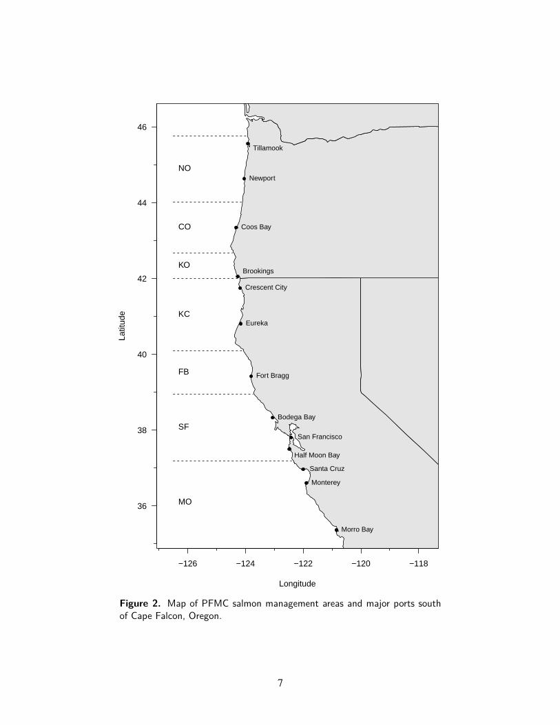
Area: The model coverage is south of Cape Falcon, Oregon, to the California / Mexico border.

SRFC fishing impacts are small north of Cape Falcon (O’Farrell et al. 2013). Within this

coverage, area is stratified according to the PFMC management areas depicted in Figure 2.

The subscript a is used to denote area-specific quantities, with a ∈ {NO, CO, KO, KC, FB,

SF, MO}.

Time: The model coverage is September 1 (y− 1) through August 31 (y) in accordance with the

SRFC “biological year” described above and the definition of the SI. Within this period, time

is stratified by month. The subscript m is used to denote month-specific quantities, with m ∈

{Sep, Oct, . . . , Aug}.

Sector: The model coverage is salmon-directed fisheries, which is stratified into the commercial

and recreational sectors. The subscript x is used to denote fishing sector-specific quantities,

with x ∈ {Commercial, Recreational}.

At its core, the ocean submodel deducts September 1 (y− 1) through August 31 (y) harvest

impacts from the SI with the remaining fish constituting the river return, R (y). This simple model

of SRFC dynamics is a necessary consequence of the SI definition, which itself is a consequence of

the limitations of the data available for SRFC assessment (O’Farrell et al. 2013). For this reason,

the SHM is not fully dynamic in the sense that the modeled abundance available for ocean harvest

later in the season is independent of the magnitude and extent of the harvest that proceeded it. As

a result,

io,a,m,x = Io,a,m,x/SI, io = ∑a,m,x

io,a,m,x, (5)

and

ho,a,m,x = Ho,a,m,x/SI, ho = ∑a,m,x

ho,a,m,x. (6)

Sections 3.1 and 3.2 describe the ocean submodel in greater detail. Section 3.3 describes the

estimation of ocean submodel parameters. All model quantities at this level are fishery-specific,

however, to simplify the presentation, we omit the fishery-specific subscripts a,m,x. For the defi-

nition of all notation used in this paper, refer to Table 1.

6

−126 −124 −122 −120 −118

Longitude

36

38

40

42

44

46La

titud

e

Tillamook

Newport

Coos Bay

Brookings

Crescent City

Eureka

Fort Bragg

Bodega Bay

San Francisco

Half Moon Bay

Santa Cruz

Monterey

Morro Bay

NO

CO

KO

KC

FB

SF

MO

Figure 2. Map of PFMC salmon management areas and major ports southof Cape Falcon, Oregon.

7

Table 1. Definition of notation used in this paper (exclusive of Appendix A). For definitionof the management areas NO, CO, KO, KC, FB, SF, MO, see Figure 2 and O’Farrell et al.(2013, Table 2).

Symbol Definition

˜ Scaled quantity∗ Forecast quantityA Ocean abundancea Management area (NO, CO, KO, KC, FB, SF, MO)β Average ratioC Number of released fish in a non-retention fisheryCVI Central Valley IndexCWT Coded-wire tagD Number of days opend Days-open fisheryE EscapementF Exploitation ratef Fishing effortg Stock unit (S,K,V,N,T )H Harvesth Harvest rateI Impactsi Impact rateK Klamath River fall Chinookk Retention (keep) fisherym Month (Sep, Oct, . . . , Aug)N Non-Central Valley hatchery-origin Chinook other than Klamath River fall runn Non-retention (catch-and-release) fisheryo OceanPFMC Pacific Fishery Management Councilp Proportion of harvest that is SRFCπ Proportion of Central Valley Chinook escapement that is SRFCQ Quotaq Quota fisheryR River returnr Riverρ Proportion caught by moochingS Sacramento River fall Chinooks Release mortality rateSHM Sacramento Harvest ModelSI Sacramento IndexSRFC Sacramento River fall ChinookT Total ChinookV Central Valley hatchery-origin Chinook other than SRFCx Sector (Commercial, Recreational)y Year of forecast

8

3.1 iiiooo, hhhooo: September 1 (yyy−−−111) through December 31 (yyy−−−111) period

The SHM is used annually for assessment and management in March (y) and April (y). The fish-

eries during the September 1 (y−1) through December 31 (y−1) period have already occurred by

this time, and the monitoring data for those fisheries is available for the March (y) and April (y)

assessment. A variety of methods are used to estimate Io and Ho for this period depending on the

nature of the fishery, and the corresponding io and ho are then derived from equations (5) and (6),

respectively.

The first distinction made in the estimation methods has to do with whether the fishery was

retention or non-retention for Chinook salmon. For retention fisheries, Ho is estimated based on

SRFC CWT recoveries as described in O’Farrell et al. (2013), and Io = Ho. Mortality associated

with release of SRFC smaller than the minimum size limit in retention fisheries is not accounted

for in the SHM.

Non-retention Chinook fisheries are atypical, but do sometimes occur. Examples include non-

retention genetic stock identification studies and Oregon coho-only fisheries. In such cases, Ho = 0,

and

Io =C× p× s, (7)

where C is the number of released Chinook that equaled or exceeded the customary minimum size

limit for that fishery, p is the proportion of these fish that are SRFC, and s is the release mortality

rate. The value C may be known (e.g., research studies with a known number of fish sampled) or

estimated (e.g., on-board observer data or angler interview data). In cases where data for C do not

exist, Io is predicted using the methods described in Section 3.2, noting that Io = SI× io. The value

p may be estimated (e.g., genetic stock identification data), or predicted (e.g., average historical

p for that fishery adjusted for current year forecasts of stock complex component abundances

(Section 3.3.3)). The value s is assumed to be a known fixed value for commercial and recreational

fisheries, with the exception of recreational fisheries in the SF and MO areas, where s depends on

the prevalence of mooching versus trolling (Section 3.3.4).

If for a given area-month-sector, the fishery was retention for a portion of the month, and

non-retention for a different portion of the month (non-overlapping time periods), the respective

9

quantities are determined as described above and then summed for the month.

3.2 iiiooo, hhhooo: January 1 (yyy) through August 31 (yyy) period

While some of the fisheries during this period have occurred prior to use of the SHM in March (y)

and April (y), the associated monitoring data is typically unavailable for this purpose. A variety

of methods are thus used to forecast the fishery-specific io and ho for this period depending on the

nature of the fishery, and the corresponding Io and Ho are then derived implicitly using equations (5)

and (6), respectively.

Ocean salmon fisheries south of Cape Falcon, Oregon are regulated either by the number of

“days open” or by “quota” (catch ceiling) within an area-month-sector fishery stratum. Both

types of regulation may be retention or non-retention although, as mentioned above, Chinook non-

retention fisheries have occurred relatively infrequently in this region. The SHM ocean submodel

allows for all four of these regulations within an area-month-sector fishery stratum, as long as they

are non-overlapping within this time period.

The harvest rate for a days-open fishery, hdo , is forecast as

hdo = β

h f ×βf D×Dk, (8)

where β h f is the average harvest rate per unit of effort, β f D is the average effort per day open, and

Dk is the number of days open in a retention fishery. For a quota fishery, the harvest rate, hqo, is

forecast as

hqo = (Qk× p)/SI, (9)

where Qk is the quota (number of Chinook) in a retention fishery, and p is the proportion of

Chinook harvest that is SRFC. The harvest rate forecast for the entire area, month, and sector is

ho = hdo +hq

o.

The impact rate for the fishery is equal to the retention harvest rate plus the mortality rate in

non-retention (n) fisheries. Thus,

io = ho +[(hd,no +hq,n

o )× s], (10)

10

where hd,no and hq,n

o are determined from equations (8) and (9), respectively, with Dn and Qn sub-

stituted for Dk and Qk, respectively.

Month, area, and sector specific impact rates are then summed over all fisheries to determine

the overall io term in equation (3), as described in equation (5).

Thus, the io and ho are a function of the (1) forecast SI, (2) estimated parameters β f D, β h f ,

p, s, and (3) management control variables Dk, Dn, Qk, Qn. The SI forecast and estimated model

parameters are updated annually just prior to the development of PFMC management measures,

while the management control variables depend on the set of management measures under consid-

eration. The method used to forecast the SI is described annually in the PFMC Preseason I report

(e.g., PFMC 2013a). The next section describes the methods that are used annually to estimate the

parameters β h f , β f D, p, and s.

3.3 Parameter estimation

3.3.1 βββfff DDD: average effort per day open

Portions of this section borrow heavily from Mohr (2006b).

For days open fisheries, the average effort per day open, β f D, is estimated separately for each

area-month-sector from the historical time series of fishing effort f and number of days open to

fishing D. These data are displayed in Figures 3 and 4 for the commercial and recreational sectors,

respectively, where each point within a panel represents the data from an individual year. The ratio

estimator (Appendix A),

βf D =

average{ f}average{D}

, (11)

where the averages are taken over the historical data, is used to estimate β f D because it is the

slope of the best fitting (in a least-squares sense) zero-intercept line through these data under the

assumption that the residual error in f is additive, with mean zero and variance proportional to D,

which appears to be appropriate for these data.

The fitted lines with slopes equal to the estimated β f D are shown in Figures 3 and 4. Note

that fishing effort is defined for the commercial sector in vessel day units while for the recreational

11

JanN

OC

OK

OK

CF

BS

FM

OFeb

0 15 30

0.0

0.5

1.0

1.5

Mar

0 15 30

0.0

0.5

1.0

1.5

0 15 30

0.00

00.

010

0 15 30

0.0

0.4

0.8

1.2

Apr

0 15 30

0.0

0.4

0.8

1.2

0 15 30

0.00

00.

010

0.02

0

0 15 30

01

23

0 15 30

0.00

0.04

0.08

0 15 30

0.0

0.5

1.0

1.5

May

0 15 30

01

23

40 15 30

0.0

0.2

0.4

0 15 30

01

23

4

0 15 30

02

46

8

0 15 30

02

46

0 15 30

0.0

1.0

2.0

Jun

0 15 30

01

23

4

0 15 30

0.0

0.4

0.8

0 15 30

0.0

1.0

2.0

0 15 30

01

23

45

0 15 30

02

46

8

0 15 30

01

23

45

0 15 30

02

46

8

Jul

0 15 30

02

46

8

0 15 30

0.0

0.2

0.4

0.6

0 15 30

0.0

0.4

0.8

0 15 30

02

46

0 15 30

02

46

8

0 15 30

01

23

4

0 15 30

02

46

Aug

0 15 30

02

46

0 15 30

0.0

0.4

0.8

0 15 30

0.0

0.5

1.0

1.5

0 15 300

12

34

5

0 15 30

01

23

45

0 15 30

0.0

1.0

2.0

Days open

Effo

rt /

1000

Commercial fishery

Figure 3. Commercial sector fishing effort plotted as a function of days open to fishing by managementarea and month. Effort is in vessel day units. See text for description of symbols, lines, and color coding.

12

JanN

OC

OK

OK

CF

BS

FM

OFeb

0 15 30

−1.

00.

01.

0

0 15 30

0.0

0.4

0.8

0 15 30

02

46

0 15 30

01

23

4

0 15 30

0.00

0.04

0.08

Mar

0 15 30

0.00

0.02

0.04

0 15 30

−1.

00.

01.

0

0 15 30

0.0

0.4

0.8

1.2

0 15 30

05

1015

0 15 30

05

1015

0 15 30

0.0

0.2

0.4

Apr

0 15 30

0.00

0.10

0.20

0 15 30

0.0

1.0

2.0

0 15 30

05

1015

0 15 30

010

2030

0 15 30

0.0

1.0

2.0

May

0 15 30

0.0

0.4

0.8

1.2

0 15 300

24

6

0 15 30

02

46

0 15 30

01

23

45

0 15 30

05

1015

0 15 30

010

30

0 15 30

05

1015

20

Jun

0 15 30

05

1015

0 15 30

05

1015

20

0 15 30

05

1525

0 15 30

04

812

0 15 30

05

1015

0 15 30

010

2030

0 15 30

020

40

Jul

0 15 30

010

2030

40

0 15 30

010

2030

0 15 30

010

30

0 15 30

04

812

0 15 30

020

40

0 15 30

010

30

0 15 30

020

40

Aug

0 15 30

05

1525

0 15 30

05

1015

0 15 30

05

1020

0 15 300

24

68

0 15 30

05

1020

0 15 30

04

812

Days open

Effo

rt /

1000

Recreational fishery

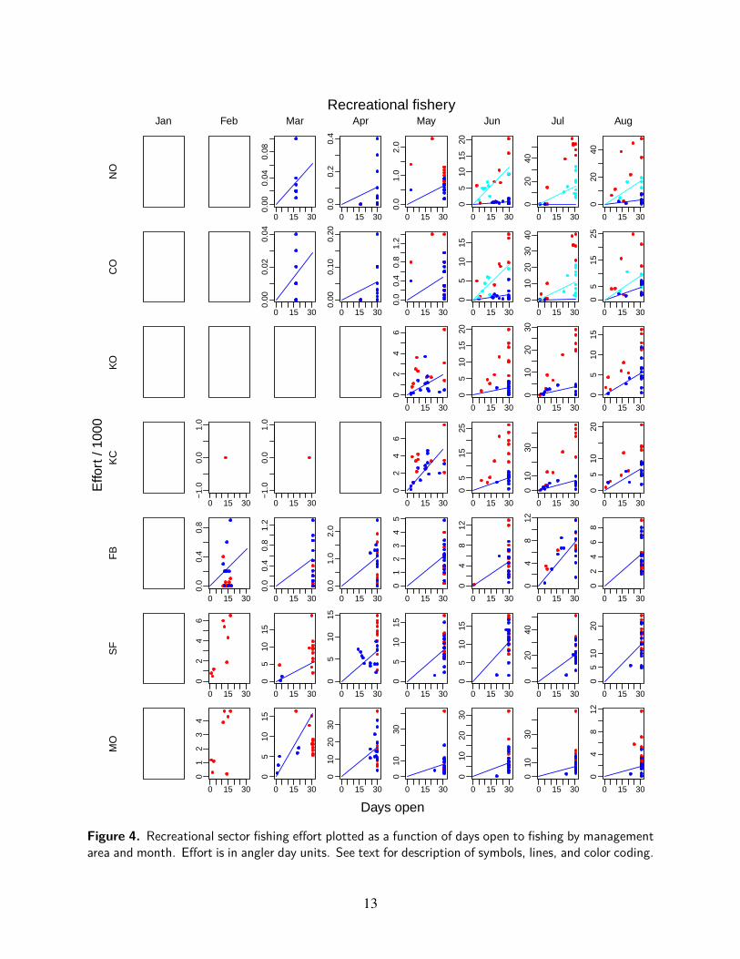
Figure 4. Recreational sector fishing effort plotted as a function of days open to fishing by managementarea and month. Effort is in angler day units. See text for description of symbols, lines, and color coding.

13

sector it is in angler day units, so that the estimated β f D (line slopes) are not directly compara-

ble across the two sectors. Color coding of the data and lines corresponds to alternative subsets

and treatments of the data considered for the purpose of improving the applicability of the β f D

estimates. A description of these subsets and treatments follows. We also note that these same

estimates of the average fishing effort per day open are used not only for the SHM, but for other

west coast salmon harvest models as well (Mohr 2006a; O’Farrell et al. 2012).

Effort data: limited to 1998–forward

Commercial fishing capacity south of Cape Falcon, Oregon, as indexed by the number of boats

making landings, has declined since the early 1980s (PFMC 2013b, Tables D-12 and D-13), and

the recreational sector has been increasingly restricted since the early 1990s. For these reasons,

effort data from 1991–forward had been used to estimate β f D for use in harvest models through

management year 2011. After management year 2011, an analysis of recent trends in effort per day

and the performance of effort predictions concluded that including effort data from the early 1990s

in the estimation of β f D led to frequent over-prediction of effort, and that the early 1990s data no

longer represented the current state of the fishing fleets (M.R. O’Farrell, unpublished data). As

a result, beginning with management year 2012, data prior to 1998, denoted by red circles, were

excluded from the estimation of β f D for both the commercial and recreational sectors.

Commercial sector: accounting for effort transfer

The commercial sector is characterized by increased mobility relative to the recreational sector,

resulting in the transfer of fishing effort across management area boundaries. As a result, the clo-

sure of certain management areas would not result in an expected loss of total effort in many cases

because much of the effort would be redistributed to nearby, open management areas. To account

for such effort transfers, fishery “types” have been defined to classify the effort data according to

the configuration of open and closed fisheries under which it occurred.

Type 0 fisheries are denoted by dark blue dots and lines in Figure 3. For the NO and CO areas,

Type 0 corresponds to data collected when both management areas were open simultaneously.

For the KO and KC areas, Type 0 fisheries are the default, and all data used for effort estimation

14

purposes is designated as Type 0. For the FB, SF, and MO area, Type 0 corresponds to data

collected when FB is closed but SF and MO are open simultaneously. This fishery configuration

for the three southernmost management areas has occurred frequently as FB has experienced more

closures than management areas further to the south.

Type 1 fisheries are defined only for the FB, SF, and MO areas, and are denoted by the light

blue dots, triangles, and lines. Type 1 fisheries correspond to data (dots) collected when these

three management areas were open simultaneously. Upon initial identification and implementation

of Type 1 fisheries, Mohr (2006b) noted that little or no contemporary effort data were available

for FB owing to frequent closures. As a result, it was assumed that if FB, SF, and MO were to be

open simultaneously, effort in FB would originate entirely from the SF and MO areas, and that total

effort would be distributed among FB, SF, and MO in the same proportions as estimated for years

1986–1991. During the 1986-1991 period, the three management areas were open simultaneously

and the data from these years was used to infer the future spatial distribution of effort under this

commercial fishery configuration. The result of distributing the pool of SF and MO effort to FB, SF,

and MO is represented by the light blue triangles. Since the first implementation of this approach

in 2002, there have been several Type 1 fisheries that have contributed data to the magnitude and

distribution of effort across FB, SF, and MO. The assumed data point denoted by the light blue

triangle continues to be treated as a “real” data point for purposes of estimating β f D, noting that

as data has accumulated, the influence of this assumed datum has diminished (Mohr 2006b).

Type 2 fisheries are defined for the NO and CO areas in Oregon and the FB, SF, and MO areas

in California. For NO and CO, a Type 2 fishery results when only one of the two areas is open,

and it is assumed that the total effort expected when both areas are open simultaneously will fully

transfer into the single open area. For the FB, SF, and MO areas, Type 2 fisheries also result when

only one of these management areas is open and the other two are closed. It is assumed that the

effort pool in the SF and MO areas (mentioned in the description of Type 1 fisheries) will fully

shift to the single open area. Type 2 fisheries are denoted by green dots, lines, and triangles, where

the triangles again represent an assumed data point based on the expected effort transfer.

15

Recreational sector: accounting for coho fishing opportunity

The recreational sector is characterized by reduced mobility relative to the commercial sec-

tor, resulting in little transfer of fishing effort across management area boundaries. Hence, an

accounting for effort shifts resulting from patterns of closed and open areas, as described for the

commercial sector, does not occur for the recreational sector. Fishery types for the recreational

sector instead pertain to Chinook-only fisheries, and in NO and CO, fisheries where coho salmon

(Oncorhynchus kisutch) retention is also allowed.

Type 0 fisheries are denoted by dark blue dots and lines in Figure 4. This is the default fishery

type for recreational Chinook fisheries.

Type 1 fisheries are defined only for the NO and CO areas in months June–August, and are

denoted by the light blue dots and lines. It has been noted for these management areas that when

coho retention is allowed, the effort per day open can be substantially higher relative to Chinook-

only fisheries. As a result, Type 1 fisheries result for the aforementioned management areas and

months when coho fishing opportunity exists. Coho fishing opportunity may also occur in the KO

management area, but this has not affected the effort response as in the more northern Oregon

management areas. Coho retention is prohibited in California.

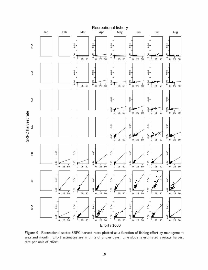
3.3.2 βββhhh fff : average harvest rate per unit effort

The average harvest rate per unit effort, β h f , is estimated separately for each area-month-sector

from the historical time series of SRFC harvest rates ho and fishing effort f . The harvest rates

themselves were determined using equation (6), where the time series of Ho and SI were estimated

as described in O’Farrell et al. (2013). The ho and f data are displayed in Figures 5 and 6 for the

commercial and recreational sectors, respectively, where each point within a panel represents the

data from an individual year. The ratio estimator (Appendix A),

βh f =

average{ho}average{ f}

, (12)

where the averages are taken over the period 1983–forward, is used to estimate β h f because it is

the slope of the best fitting (in a least-squares sense) zero-intercept line through these data under

16

the assumption that the residual error in ho is additive, with mean zero and variance proportional

to f , which appears to be appropriate for these data.

The fitted lines with slopes equal to the estimated β h f are shown in Figures 5 and 6. Note that

the within-sector panels have the same axes scales, and thus the estimated β h f (lines slopes) within

a sector are directly comparable across the areas and months in these figures.

Harvest rates per unit effort are a function of the SRFC spatial distribution and catchability.

Estimated β h f tend to be highest in the FB, SF, and MO management areas for both the commercial

and recreational sectors. For the recreational sector, estimates of β h f are much lower in Oregon

management areas relative to California. As a result, a single unit of fishing effort, for both sectors,

in the southern management areas results in higher expected SRFC harvest and impact rates.

3.3.3 ppp: SRFC stock proportion

Forecasts of the SRFC stock proportion in the harvest p, stratified by area, month, and sector,

are needed for predicting SRFC harvest and impacts in quota and non-retention fisheries. While

these types of fisheries are relatively rare in ocean fisheries south of Cape Falcon, and have not

historically accounted for the bulk of SRFC impacts, forecasts of p are nevertheless made for all

strata.

Estimates of historical harvest have been made for two stocks (S: SRFC, and K: Klamath

River fall Chinook) and two stock groups (V : Central Valley hatchery-origin Chinook stocks other

than SRFC, and N: non-Central Valley hatchery-origin Chinook stocks other than Klamath River

fall run) for all area-month-sectors from 1983–forward (for details regarding these stock units

and the estimation of their harvest see O’Farrell et al. 2013). In combination, these stock units

(g = S,K,V,N) account for the large majority of ocean Chinook harvest south of Cape Falcon,

Oregon, and it is assumed in the estimation of these harvests that they constitute the entire harvest.

For a particular stratum and year p is a function of the spatial distribution and catchability of

SRFC, but also the relative abundance of the other stock units contributing to the total harvest.

Recognizing this, p is forecast separately for each area-month-sector from the historical stock

17

JanN

OC

OK

OK

CF

BS

FM

OFeb

0.00

0.06

0.12

0 4 8

Mar

0.00

0.06

0.12

0 4 8

0.00

0.06

0.12

0 4 8

0.00

0.06

0.12

0 4 8

Apr

0.00

0.06

0.12

0 4 8

0.00

0.06

0.12

0 4 8

0.00

0.06

0.12

0 4 8

0.00

0.06

0.12

0 4 8

0.00

0.06

0.12

0 4 8

0.00

0.06

0.12

0 4 8

May

0.00

0.06

0.12

0 4 8

0.00

0.06

0.12

0 4 80.

000.

060.

12

0 4 8

0.00

0.06

0.12

0 4 8

0.00

0.06

0.12

0 4 8

0.00

0.06

0.12

0 4 8

Jun

0.00

0.06

0.12

0 4 8

0.00

0.06

0.12

0 4 8

0.00

0.06

0.12

0 4 8

0.00

0.06

0.12

0 4 8

0.00

0.06

0.12

0 4 8

0.00

0.06

0.12

0 4 8

0.00

0.06

0.12

0 4 8

Jul

0.00

0.06

0.12

0 4 8

0.00

0.06

0.12

0 4 8

0.00

0.06

0.12

0 4 8

0.00

0.06

0.12

0 4 8

0.00

0.06

0.12

0 4 8

0.00

0.06

0.12

0 4 8

0.00

0.06

0.12

0 4 8

Aug

0.00

0.06

0.12

0 4 8

0.00

0.06

0.12

0 4 8

0.00

0.06

0.12

0 4 8

0.00

0.06

0.12

0 4 80.

000.

060.

12

0 4 8

0.00

0.06

0.12

0 4 8

Effort / 1000

SR

FC

har

vest

rat

eCommercial fishery

Figure 5. Commercial sector SRFC harvest rates plotted as a function of fishing effort by managementarea and month. Effort estimates are in units of vessel days. Line slope is estimated average harvestrate per unit of effort.

18

JanN

OC

OK

OK

CF

BS

FM

OFeb

0.00

0.04

0 25 50

0.00

0.04

0 25 50

0.00

0.04

0 25 50

0.00

0.04

0 25 50

Mar

0.00

0.04

0 25 50

0.00

0.04

0 25 50

0.00

0.04

0 25 50

0.00

0.04

0 25 50

0.00

0.04

0 25 50

Apr

0.00

0.04

0 25 50

0.00

0.04

0 25 50

0.00

0.04

0 25 50

0.00

0.04

0 25 50

0.00

0.04

0 25 50

May

0.00

0.04

0 25 50

0.00

0.04

0 25 500.

000.

04

0 25 50

0.00

0.04

0 25 50

0.00

0.04

0 25 50

0.00

0.04

0 25 50

0.00

0.04

0 25 50

Jun

0.00

0.04

0 25 50

0.00

0.04

0 25 50

0.00

0.04

0 25 50

0.00

0.04

0 25 50

0.00

0.04

0 25 50

0.00

0.04

0 25 50

0.00

0.04

0 25 50

Jul

0.00

0.04

0 25 50

0.00

0.04

0 25 50

0.00

0.04

0 25 50

0.00

0.04

0 25 50

0.00

0.04

0 25 50

0.00

0.04

0 25 50

0.00

0.04

0 25 50

Aug

0.00

0.04

0 25 50

0.00

0.04

0 25 50

0.00

0.04

0 25 50

0.00

0.04

0 25 500.

000.

04

0 25 50

0.00

0.04

0 25 50

Effort / 1000

SR

FC

har

vest

rat

eRecreational fishery

Figure 6. Recreational sector SRFC harvest rates plotted as a function of fishing effort by managementarea and month. Effort estimates are in units of angler days. Line slope is estimated average harvestrate per unit of effort.

19

proportion estimates as

p = average{p}, (13)

where the average is taken over the period 1983–forward, and p is a given year’s proportion of

SRFC in the harvest adjusted for each stock unit’s current year ocean abundance forecast, A∗g,

relative to its estimated ocean abundance at the time, Ag:

p =Ho,S

(A∗S/AS

)∑g Ho,g

(A∗g/Ag

) , (14)

where Ho,g is the harvest of stock unit g, and the sum is over g= S,K,V,N. A∗S is the forecast SI and

A∗K is the aggregate-age ocean abundance forecast for Klamath River fall Chinook. The A∗S and A∗K

forecasts and the time series of {AS} and {AK} estimates are provided in PFMC (2013a). Forecasts

of A∗V and A∗N and the time series of {AV} and {AN} estimates are produced and maintained by the

California Department of Fish and Wildlife, Ocean Salmon Project, as part of the annual stock

assessment process.

3.3.4 sss: release mortality rate

Estimates of the release mortality rate, s, are needed for forecasting impacts in non-retention fish-

eries. When the method of fishing is trolling, the release mortality rate is assumed equal to 0.26

and 0.14 for the commercial and recreational sectors, respectively, as recommended by the PFMC

Salmon Technical Team (STT 2000) based on their review of west coast salmon hook and release

mortality studies.

Recreational fisheries in the SF and MO management areas have, to varying degrees over time,

also employed a method of fishing known as “mooching” in lieu of trolling. Mooching in this re-

gion typically consists of drifting a bait rigged with either a single or double hook. The prevalence

of gut hooking has been shown to be higher for mooching than trolling, which leads to increased

release mortality under this method of fishing. Grover et al. (2002) estimated a release mortality

rate of 0.422 when the method of fishing is mooching with barbless circle hooks (the mooching

gear requirement currently in place). Therefore, for the recreational sector in the SF and MO areas,

the release mortality rate for a particular area-month is a weighted average of the mooching and

20

trolling release mortality rates, the weights being equal to the proportion of the harvest caught by

the respective method.

Thus,

s =

0.26, x = Commercial,

0.14, x = Recreational, a 6= {SF, MO},

(ρ×0.422)+((1−ρ)×0.14) , x = Recreational, a = {SF, MO},

(15)

where ρ is forecast as the most recent 5-year average proportion of the area-month recreational

harvest caught by mooching.

4 River Submodel

Following completion of the August ocean fisheries, the SRFC river return, R, is forecast as

R = SI× (1− io), (16)

and the river harvest submodel is then used to forecast the river fishery impact rate, ir, based on

the type of proposed river fishery. The two types of river fishery that have been employed in the

Sacramento basin are an “unconstrained” fishery and a quota fishery; a non-retention fishery has

not been used to date.

The most common type of fishery in the basin is referred to as “unconstrained”, which is

characterized by the Sacramento River and its major tributaries being open to Chinook retention

during the bulk of the SRFC migration and spawning period. However, such a fishery is not

completely unconstrained because regulations specify daily bag and possession limits, closures to

many minor tributary streams, and closures to select reaches of rivers otherwise open to Chinook

retention. For the unconstrained fishery, O’Farrell et al. (2013) estimated an average historical

harvest rate of 0.14, and the SHM thus assumes for this type of river fishery that

ir = hr = 0.14. (17)

21

Quota fisheries have been employed only when the SI forecast was low and river fishery impacts

needed to be reduced below unconstrained fishery levels. Under quota fisheries, the SHM assumes

that

ir = hr = Qkr/R, (18)

where Qkr is the river retention fishery quota size in numbers of fish.

5 Discussion

The development of the SHM, in conjunction with the SI, represented a marked improvement

over the previous SRFC assessment procedure. In contrast with the CVI-based harvest model, the

SHM (1) stratified ocean harvest by management area, month, and sector for the region south of

Cape Falcon, Oregon and (2) accounted for Sacramento basin recreational river fisheries. These

capabilities now allow the PFMC to use area-month-sector closures and quotas to more directly

control ocean harvest of SRFC. Alternative river fishery configurations can also be accounted for

in the forecasts of E and F . Neither of these management controls were available prior to the

development of the SI and SHM.

While the SHM represented a significant advance over the previous harvest model, there are

limitations to models with the SHM’s structure. The historical SRFC CWT and spawner escape-

ment data did not allow for an age-structured assessment in the form of cohort reconstructions

which precludes age-specific abundance, harvest, and escapement forecasts. One example of a

limitation resulting from an aggregate-age assessment is that it does not allow for the estimation

and forecasting of impacts associated with hook and release mortality for fish smaller than the

minimum size limit in retention fisheries. The inability of the SHM to account for this form of

release mortality does not allow the io forecast to be sensitive to changes in minimum size lim-

its, a management tool frequently used by the PFMC to achieve conservation objectives for other

salmon stocks.

The lack of age-specific accounting in the SI and SHM can lead to E and F forecast errors in

other ways as well. For example, there may be age-specific patterns in SRFC harvest rates per

22

unit effort that, when undetected, could result in poor impact rate forecast performance. With the

age-structured Klamath River fall Chinook assessment, for example, there are notable differences

between the age-3 and age-4 contact rates per unit effort in the commercial sector, and in some

areas and months in the recreational sector. This age structure effect is readily accounted for in the

Klamath Ocean Harvest Model yet the ability to identify and respond to those differences does not

exist for the SHM. In addition, there are likely large differences in age-specific maturation rates for

SRFC that are not recognized in the SI and SHM. An aggregate-age index of abundance will be

composed of different relative contributions of the age-3 and age-4 cohorts as a result of variable

year class strength. The fraction of the total index that will mature in that year will vary from year

to year inasmuch as the underlying age structure and the age-specific maturation rates differ. Such

processes likely have effects on forecast performance, though the magnitude of those effects are

not known.

The use of the SI and SHM is likely to be an interim assessment for SRFC, bridging the gap to

an age-structured approach. Beginning in 2006 a “constant-fractional marking” program (Buttars

2012) was implemented. The goal of the program is to mark (adipose fin clip) and tag (CWT)

25% of SRFC hatchery production. Increased effort is also being made to improve escapement

monitoring and recover CWTs in natural spawning areas (Bergman et al. 2012). The California

Department of Fish and Wildlife has developed a scale aging program capable of estimating age-

specific run size (Grover and Kormos 2008). If these programs are appropriately and consistently

implemented, a time series of data sufficient for cohort reconstructions will eventually exist for

SRFC, and this will allow for a fully age-structured assessment similar to that for Klamath River

fall Chinook.

Acknowledgements

The initial development of the SHM took place during a very short and intense period of time,

primarily during the March 2008 PFMC meeting. In order to implement the model in time for

use in 2008 management we relied heavily on expert data analysis performed by Allen Grover and

23

Melodie Palmer-Zwahlen of the California Department of Fish and Game. Their contributions to

the SHM were, and continue to be, invaluable. This paper was also improved by comments from

Will Satterthwaite and Shanae Allen-Moran.

References

Bergman, J. M., R. M. Nielson, and A. Low (2012). Central Valley Chinook salmon in-river

escapement monitoring plan. California Department of Fish and Game Administrative Report

Number: 2012-1.

Buttars, B. (2012). Central Valley salmon and steelhead marking/coded-wire tagging program.

Pacific States Marine Fisheries Commission, 10950 Tyler Road, Red Bluff, California 96080.

Grover, A. and B. Kormos (2008). The 2007 Central Valley Chinook age-specific run size esti-

mates. Unpublished report, California Department of Fish and Game Scale Aging Program.

Grover, A., M. Mohr, and M. Palmer-Zwahlen (2002). Hook-and-release mortality of Chinook

salmon from drift mooching with circle hooks: management implications for California’s ocean

sport fishery. In J. Lucy and A. Studholme (Eds.), Catch and release in marine recreational

fisheries, American Fisheries Society, Symposium 30, Bethesda, Maryland, pp. 39–56.

Mohr, M. (2006a). The Klamath Ocean Harvest Model (KOHM): model specification. Unpub-

lished report. National Marine Fisheries Service, Santa Cruz, CA.

Mohr, M. (2006b). The Klamath Ocean Harvest Model (KOHM): parameter estimation. Unpub-

lished report. National Marine Fisheries Service, Santa Cruz, CA.

O’Farrell, M. R., S. D. Allen, and M. S. Mohr (2012). The Winter-Run Harvest Model (WRHM).

U.S. Department of Commerce, NOAA Technical Memorandum NOAA-TM-NMFS-SWFSC-

489, 17p.

O’Farrell, M. R., M. S. Mohr, M. L. Palmer-Zwahlen, and A. M. Grover (2013). The Sacra-

mento Index (SI). U.S. Department of Commerce, NOAA Technical Memorandum NOAA-

TM-NMFS-SWFSC-512, 36p.

PFMC (Pacific Fishery Management Council) (2008a). Preseason report I: Stock abundance analy-

24

sis for 2008 ocean salmon fisheries. Pacific Fishery Management Council, 7700 NE Ambassador

Place, Suite 101, Portland, Oregon 97220-1384.

PFMC (Pacific Fishery Management Council) (2008b). Preseason report II: Analysis of proposed

regulatory options for 2008 ocean salmon fisheries. Pacific Fishery Management Council, 7700

NE Ambassador Place, Suite 101, Portland, Oregon 97220-1384.

PFMC (Pacific Fishery Management Council) (2012). Pacific coast Salmon Fishery Management

Plan for commercial and recreational salmon fisheries off the coasts of Washington, Oregon, and

California as revised through Amendment 16. Pacific Fishery Management Council, Portland,

OR. 90p.

PFMC (Pacific Fishery Management Council) (2013a). Preseason report I: Stock abundance analy-

sis and environmental analysis part 1 for 2013 ocean salmon fishery regulations. Pacific Fishery

Management Council, 7700 NE Ambassador Place, Suite 101, Portland, Oregon 97220-1384.

PFMC (Pacific Fishery Management Council) (2013b). Review of 2012 ocean salmon fisheries:

stock assessment and fishery evaluation document for the Pacific Coast Salmon Fishery Man-

agement Plan. Pacific Fishery Management Council, 7700 NE Ambassador Place, Suite 101,

Portland, Oregon 97220-1384.

STT (Salmon Technical Team) (2000). STT recommendations for hooking mortality rates in 2000

recreational ocean Chinook and coho fisheries. Pacific Fishery Management Council, 7700 NE

Ambassador Place, Suite 101, Portland, Oregon 97220-1384.

Appendix A Ratio Estimation

The choice of which estimator to use when estimating the average harvest rate per unit of effort,

β h f , or average effort per day open, β f D, depends on the nature of the relationship between the nu-

merator (Y ) and denominator (X) variables of the respective ratio (β ). For each area-month-sector

stratum, we assume that the following zero-intercept, linear (ratio) model adequately characterizes

25

the relationship between the Y and X variables:

Y = βX + ε, µε = 0, σ2ε = aXb, (A-1)

where for β = β h f , Y = ho and X = f , and for β = β f D, Y = f and X = D. Under this model,

the expected value of Y increases linearly from the origin with X , and the slope of this line, β , is

the average (expected value) of Y per unit X . The residual error in Y about this linear relationship,

ε , has a mean value of 0 and a variance that is proportional to Xb, where b is a specified constant.

Figure A-1 illustrates these model features for the most commonly specified variance functions:

constant variance (b = 0), variance proportional to X (b = 1), and variance proportional to X2

(b = 2).

This variance function should be taken into account when estimating β from a particular set

of data, {X j,Yj}, and one technique for doing this is to use the method of weighted least squares,

where each observation is weighted inversely proportional to its residual variance in the sum of

squared-errors function:

SS(β ) = ∑j

w j(Yj− Y j)2 = ∑

j

(Yj− βX j)2

Xbj

= ∑j

Y 2j X−b

j −2β ∑j

Y jX1−bj + β

2∑

jX2−b

j . (A-2)

The value of β that minimizes SS(β ) is the weighted least squares estimator of β , and it can be

found by setting the derivative of SS(β ) with respect to β ,

dSS(β )

dβ=−2∑

jYjX1−b

j +2β ∑j

X2−bj , (A-3)

to zero and solving for β , giving

β =∑ j YjX1−b

j

∑ j X2−bj

. (A-4)

For the specific values b = 0, 1, 2, this results in the following estimators for β :

β =

∑ j Y jX j

∑ j X2j, b = 0 : ordinary (unweighted) least-squares estimator

∑ j Y j/n∑ j X j/n , b = 1 : “ratio of means” (ratio estimator)

∑ j Y j/X jn , b = 2 : “mean of ratios”,

(A-5)

26

0.0 0.2 0.4 0.6 0.8 1.0

0.0

0.5

1.0

1.5

X

Y

b = 0

0.0 0.2 0.4 0.6 0.8 1.0

0.0

0.5

1.0

1.5

X

Y

b = 1

0.0 0.2 0.4 0.6 0.8 1.0

0.0

0.5

1.0

1.5

X

Y

b = 2

Figure A-1. Illustration of the ratio model defined by equation (A-1) for specified values b = 0,1,2,respectively. Solid line is the expected value of Y ; dashed lines are the expected value ± two standarddeviations. To highlight the effect of b in the model, the slope of the expected value line is equal (β = 1)in all panels, as is the residual variance at X = 0.25 (σ2

ε = 0.01).

where n is the number of {X j,Yj} data points.

Based on the data patterns exhibited in the area-month-sector specific panels of Figures 3, 4, 5,

and 6, we conclude that the ratio model with b = 1 provides the most apt description of these data,

and that β is therefore most appropriately estimated using the ratio estimator.

27

RECENT TECHNICAL MEMORANDUMSSWFSC Technical Memorandums are accessible online at the SWFSC web site (http://swfsc.noaa.gov). Copies are also available from the National Technical Information Service, 5285 Port Royal Road, Springfield, VA 22161 (http://www.ntis.gov). Recent issues of NOAA Technical Memorandums from the NMFS Southwest Fisheries Science Center are listed below:

NOAA-TM-NMFS-SWFSC-

515

516

517

518

519

520

521

522

523

524

Photographic guide of pelagic juvenile rockfish (SEBASTES SPP.) and other fishes in mid-water trawl surveys off the coast of California.SAKUMA, K. M., A. J. AMMANN, and D. A. ROBERTS(July 2013)

Form, function and pathology in the pantropical spotted dolphin (STENELLAATTENUATA).EDWARDS, E. F., N. M. KELLAR, and W. F. PERRIN(August 2013)

Summary of PAMGUARD beaked whale click detectors and classifiers used during the 2012 Southern California behavioral response study.KEATING, J. L., and J. BARLOW(September 2013)

Seasonal gray whales in the Pacific northwest: an assessment of optimumsustainable population level for the Pacific Coast Feeding Group.PUNT, A. E., and J. E. MOORE(September 2013)

Documentation of a relational database for the Oregon sport groundfish onboard sampling program.MONK, M. E., E. J. DICK, T. BUELL, L. ZUMBRUNNEN, A. DAUBLE and D. PEARSON(September 2013)

A fishery-independent survey of cowcod (SEBASTES LEVIS) in the Southern CA bight using a remotely operated vehicle (ROV).

STIERHOFF, K. L., S. A. MAU, and D. W. MURFIN

(September 2013)

Abundance and biomass estimates of demersal fishes at the footprint and piggy bank from optical surveys using a remotely operated vehicle (ROV).

STIERHOFF, K. L., J. L. BUTLER, S. A. MAU, and D. W. MURFIN(September 2013)

Klamath-Trinity basin fall run chinook salmon scale age analysis evaluation.

SATTERTHWAITE, W. H., M. R. O’FARRELL, and M. S. MOHR

(September 2013)

AMLR 2010-2011 field season report.

WALSH, J. G., ed.

(February 2014)

Status review of the Northeastern Pacific population of white sharks (CARCHARODON CARCHARIAS) under the endangered species act.DEWAR, H., T. EGUCHI, J. HYDE, D. KINZEY, S. KOHIN, J. MOORE, B. L. TAYLOR, and R. VETTER(December 2013)