Report No. CG-D-12-92 AD-A252 345

SPRING 1985 LEEWAY EXPERIMENT

Louis Nashand

James Willcox

U.S. Coast Guardl esearch and Development Center

1082 Shennecossett RoadGroton, CT 06340-6096

RNAL REPORT DTICOCTOBER 1991

, 29 uThis document Is available to the U.S. public through theNational Technical Information Service, Spuingfield, Virginia 22161

Prepared for:

U.S. Department Of TransportationUnited States Coast GuardOffice of Engineering, Logistics, and DevelopmentWashington, DC 20593a-D001

92-1673392 6 24 079 I11111111l1l1111!1

• III

NOTICE !

I

This document Is disseminated under the sponsorship of theDepartment of Transportation in the Interest of information Iexchange. The United States Government assumes noliability for its contents or use thereof.

The United States Government does not endorse products ormanufacturers. Trade or manufacturers' names appear hereinsolely because they are considered essential to the object ofthis report. 3

The contents of this report reflect the views of the Coast IGuard Research and Development Center, which Isresponsible for the facts and accuracy of data presented.This report does not constitute a standard, specification, orregulation.

AMUEL F. POWEL, ITechnical DirectorU.S. Coast Guard Research and Development Center IAvery Point, Groton, Connecticut 06340-6096

II

I

ii I

Technical Report Documentation Page1. Report No. 2. Government Accession No. 3. Recipient's Catalog No.

GG-D-12-92 1

4. Title and Subtitle 5. Report DateOctober 1991

SPRING 1985 LEEWAY EXPERIMENT 6. Performing Organization Code

8. Performing Organization Report No.7. Author(s) R&DC 01/88

Louis Nash and James Willcox9. Performing Organization Name and Address 10. Work Unit No. (TRAIS)U.S. Coast GuardResearch and Development Center 11. Contract or Grant No.1082 Shennecossett RoadGroton, Connecticut 06340-6096 13. Type of Report and Period Covered

12. Sponsoring Agency Name and AddressDepartment of Transportation FINALU.S. Coast GuardOffice of Engineering, Logistics, and Development 14. Sponsoring Agency CodeWashington, D.C. 20593-0001

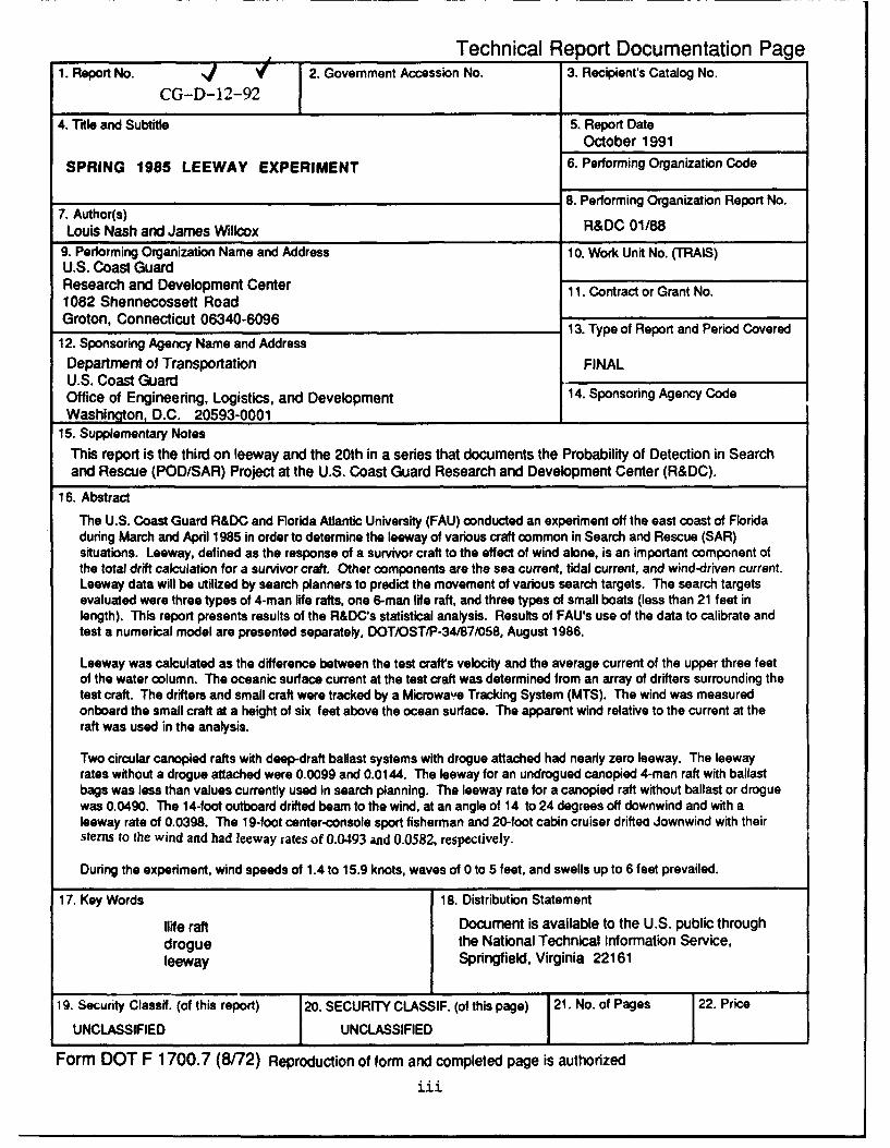
15. Supplementary NotesThis report is the third on leeway and the 20th in a series that documents the Probability of Detection in Searchand Rescue (POD/SAR) Project at the U.S. Coast Guard Research and Development Center (R&DC).

16. Abstract

The U.S. Coast Guard R&DC and Florida Atlantic University (FAU) conducted an experiment off the east coast of Floridaduring March and April 1985 in order to determine the leeway of various craft common in Search and Rescue (SAR)situations. Leeway, defined as the response of a survivor craft to the effect of wind alone, is an important component ofthe total drift calculation for a survivor craft. Other components are the sea current, tidal current, and wind-driven current.Leeway data will be utilized by search planners to predict the movement of various search targets. The search targetsevaluated were three types of 4-man life rafts, one 6-man life raft, and three types of small boats (less than 21 feet inlength). This report presents results of the R&DC's statistical analysis. Results of FAU's use of the data to calibrate andtest a numerical model are presented separately, DOT/OST/P-34/87/058, August 1986.

Leeway was calculated as the difference between the test craft's velocity and the average current of the upper three feetof the water column. The oceanic surface current at the test craft was determined from an array of drifters surrounding thetest craft. The drifters and small craft were tracked by a Microwave Tracking System (MTS). The wind was measuredonboard the small craft at a height of six feet above the ocean surface. The apparent wind relative to the current at theraft was used in the analysis.

Two circular canopied rafts with deep-draft ballast systems with drogue attached had nearly zero leeway. The leewayrates without a drogue attached were 0.0099 and 0.0144. The leeway for an undrogued canopied 4-man raft with ballastbags was less than values currently used in search planning. The leeway rate for a canopied raft without ballast or droguewas 0.0490. The 14-foot outboard drifted beam to the wind, at an angle of 14 to 24 degrees off downwind and with aleeway rate of 0.0398. The 19-foot center-console sport fisherman and 20-foot cabin cruiser driftea Jownwind with theirsterns to the wind and had leeway rates of 0.0493 and 0.0582, respectively.

During the experiment, wind speeds of 1.4 to 15.9 knots, waves of 0 to 5 feet, and swells up to 6 feet prevailed.

17. Key Words 18. Distribution Statement

life raft Document is available to the U.S. public throughdrogue the National Technical Information Service,leeway Springfield, Virginia 22161

19. Security Classif. (of this report) 20. SECURITY CLASSIF. (of this page) 21. No. of Pages 22. Price

UNCLASSIFIED I UNCLASSIFIED

Form DOT F 1700.7 (8/72) Reproduction of form and completed page is authorized

iii£

V 0

co, >.

t .o .2020 -

Cr crc 0 0 0)

Q. 00 N 0o m

00aj W 0 00 v 0~ C 00 N 'o C r

0 0U I> 0 o

.9 CL ) - 0

CD z) I-

0c c~ 00

E 12 E r874 M 0 0

0 0~

0 cc L z 1 et 9t L& I L c I L 6 9 L 19 * 1 L U

O 9 8 71 6 5 4 3 2 1 nhes

Qo (D .0 E-E-EEEL-0 E 0

cc 2

IE(0 IN(0 CIO

- (0 ~~(o ( 0(0

o t c c 0 0m: L0L

75 LU cl0 0 l <0 72o) > cc 'CY '

0- - 0- c 0

2~ C CoY

000 (D4 ) .

iv 0

ACKNOWLEDGMENTS

The assistance of many individuals made this research

possible, especially the team from FAU under Dr. T. C. Su and Dr.

F.S. Hotchkiss, and the crew of the R/V BELLOWS under Captain W.

Millender from the Florida Institute of Oceanography. The

Department of Transportation (DOT) Office of University Research

provided the opportunity for the cooperative effort.

Special thanks go to R&D field team members Art Allen, Mike

Couturier, Rick Sager, and Tim Noble. Mike was responsible for

programming the tracking system and a good portion of the

analysis programs. Rick and Tim were the hands-on personnel.

Finally, the assistance of Dr. D. F. Paskausky, Dr. D. L.

Murphy, and Mr. Larry Nivert is gratefully acknowledged.

Aooession For

NTIS QRA&I

DTIC TAB QUnannounced QJustification

By.Distribution/

Availability Codes

Avail and/orDist Special

v

lI

LIST OF ACRONYMS

CASP Computer Assisted Search Planning 3CTTO Canadian Central Tactics and Trials Orgaiiization

DLR Downwind Leeway Rate

DOT Department of Transportation

FAU Florida Atlantic University

LA Leeway Angle IMTS Microwave Tracking System

N/A Not Applicable 3NPL National Physics Laboratory

POD/SAR Probability of Detection/Search and Rescue

R&DC Research and Development Center

rms root mean square

RWD Relative Wind Direction

SAR Search and Rescue

XBT Expendable Bathythermograph 3IiiIiIi

vi 3

TABLE OF CONTENTS

Pagie

ACKNOWLEDGMENTS........................................... v

LIST OF ACRONYMS.......................................... vi

EXECUTIVE SUMMARY......................................... ES-i

CHAPTER 1 - INTRODUCTION................................. 1

1.1 SCOPE ................................................ 11.2 BACKGROUND........................................... 3

1.2.1 Leeway in Search and Rescue....................... 31.2.2 Previous Leeway Investigations.................... .6

CHAPTER 2 - THE EXPERIMENT............................... .15

2.1 DESIGN AND CONDUCT.................................. 15

2.1.1 Position........................................... .182.1.2 Test Craft's Instrument Packages.................. 202.1.3 R/V OCEANEER IV.................................... .212.1.4 R/V BELLOWS......................................... 222.1.5 Environmental Buoy................................. 22

2.2 DRIFTERS............................................. 23

2.3 TEST CRAFT........................................... 23

2.3.1 Simulation of Life Raft Complement................ 242.3.2 Switlik 4-Man Life Raft........................... .242.3.3 Givens Buoy 6-Man Life Raft....................... 252.3.4 Avon 4-Man Life Raft............................... 282.3.5 Winslow 4-Man Life Raft........................... .282.3.6 14-Foot Outboard................................... .302.3.7 19-Foot Outboard................................... .302.3.8 20-Foot Cabin Cruiser.............................. 30

CHAPTER 3 - DATA PROCESSING.............................. 33

3.1 INTRODUCTION......................................... 33

3.2 CALCULATION OF CURRENTS, TEST CRAFT VELOCITIES,

AND LEEWAY........................................... 33

3.3 WIND DATA............................................ 34

3.4 DATA COLLATION....................................... 35

vii

I

TABLE OF CONTENTS (Cont'd.) IPage1

3.5 LEEWAY ANGLE ...................................... 35

CHAPTER - 4 ANALYSIS ............................... 37

4.1 INTRODUCTION ...................................... 37

4.1.1 Significance of Parameters .................... 37U4.1.2 Leeway Models .................................... 40

4.2 SWITLIK 4-MAN LIFE RAFT ........................... 40

4.2.1 Switlik 4-Man Raft With Drogue ................ 404.2.2 Switlik 4-Man Raft Without Drogue ............. 46

4.3 GIVENS 6-MAN LIFE RAFT ............................ 48

4.3.1 Givens 6-Man Raft With Drogue ................. 48 i4.3.2 Givens 6-Man Raft Without Drogue .............. 49

4.4 AVON 4-MAN LIFE RAFT .............................. 57 34.4.1 Summary for Avon 4-Man Raft ................... 60

4.5 WINSLOW 4-MAN LIFE RAFT ........................... 62 14.5.1 Winslow 4-Man Raft With Drogue ................ 634.5.2 Winslow 4-Man Raft Without Drogue ............. 634.5.3 Winslow 4-Man Raft Without Drogue,

Fully Loaded ..................................... 63

4.6 SMALL BOATS ...................................... . . 68

4.6.1 14-Foot Outboard ................................ 684.6.2 19-Foot Outboard ................................ 72 I4.6.3 20-Foot Cabin Cruiser ........................... 75

CHAPTER - 5 CONCLUSIONS ................................. 79

5.1 SUMMARY ............................................ 79

5.2 IMPLICATIONS FOR CASP ...................................... 79

5.2.1 Canopied Rafts With Deep-Draft BallastSystem and Drogue ............................... 81

5.2.2 Canopied Rafts With Deep-Draft BallastSystem (No Drogue) ............................... 81

5.2.3 Canopied Rafts With Ballast Buckets .......... 82 I5.2.4 Canopied Rafts Without Ballast or Drogue ..... 825.2.5 Light-Displacement Small Craft and Outboards. 83

viii

TABLE OF CONTENTS (Cont'd.)

Pag9e

APPENDIX A - DATA PROCESSING METHODS.................... A-i

A.1 INTRODUCTION......................................... A-i

A.2 POSITION DATA........................................ A-2

A.2.1 Piecewise Linear Regression Method..............A-3

A.2.2 Current Calculations............................ A-5A.2.3 Current Field Calculations...................... A-6A.2.4 Velocity Calculations........................... A-7A.2.5 Leeway Calculations............................. A-7

A.3 WIND DATA............................................ A-8

A.3.1 Automated Instrument Package Data................A-8

A.3. 2 Brooks and Gatehouse Hercules 190 Data.........A-9

A.4 DATA COLLATION....................................... A-10

A.5 LEEWAY ANGLE......................................... A-10

A.6 LEEWAY COMPONENTS................................... A-10

APPENDIX B - LEEWAY MODELS AND ERROR ANALYSIS .... B-i

B.i INTRODUCTION......................................... B-i

B.2 FITTING OF LEEWAY MODELS............................ B-2

B.3 ERROR ANALYSIS.......................................B-5

APPENDIX C - OBSERVATIONS AND RECOMMENDATIONS .... C-i

C.1 PROPOSED EXPERIMENTAL METHOD OF DETERMINING

LEEWAY............................................... C-i

C.2 RESEARCH TOPICS...................................... C-2

REFERENCES................................................ R-i

ix

I

LIST OF ILLUSTRATIONS IFigure Ae 3

1 Life Raft Drift Without Drogue ................. 7

2 Life Raft Drift With Drogue .................... 7

3 Leeway Versus Wind Speed ....................... 11

4 MTS Drifter .................................... 16 15 Switlik 4-Man Life Raft With Toroid Ballast .... 26

6 Givens Buoy 6-Man Life Raft .................... 27

7 Avon 4-Man Life Raft ........................... 29 18 Winslow 4-Man Life Raft ........................ 31

9 Photographs of 20-foot Cabin Cruiser ........... 32 310 Relation of Relative Wind Direction (RWD) and

Leeway Angle (LA) .............................. 38 I11 Switlik 4-Man Life Raft With Toroid Ballast .... 42

12 RWD Versus Wind Speed for Switlik 4-Man Raft UWith Drogue .................................... 43

13 Data of 6 April 1985 for Switlik 4-Man RaftWith Drogue .................................... 44

14 Downwind Component of Leeway Versus Wind Speedfor Switlik 4-Man Raft With Drogue ............. 45

15 Downwind Component of Leeway Versus Wind Speedfor Switlik 4-Man Raft Without Drogue .......... 47

16 Givens Buoy 6-Man Life Raft .................... 50 317 RWD Versus Wind Speed for 6-Man Raft

With Drogue .................................... 51

18 Downwind Component of Leeway Speed Versus Wind ISpeed for Givens 6-Man Raft With Drogue .......... 52

19 Data of 24 March 1985 for Givens 6-Man Raft IWithout Drogue ................................. 54

20 Doanwind Component of Leeway Versus Wind Speed nfor Givens 6-Man Raft Without Drogue ........... 55

21 Avon 4-Man Life Raft ........................... 58 3x I

LIST OF ILLUSTRATIONS (cont'd)

Figureage

22 RWD Versus Wind Speed for Avon 4-Man RaftWithout Drogue ..................................... 59

23 Downwind Component of Leeway Speed Versus Wind

Speed for Avon 4-Man Raft (RWD<115R) ........... 61

24 Winslow 4-Man Raft ................................ 64

25 Downwind Component of Leeway Versus Wind Speedfor Winslow 4-Man Raft Without Drogue,Fully Loaded ....................................... 65

26 Leeway Angle Versus Wind Speed for 14-FootOutboard ...... .................................... 70

27 Primary Component of Leeway Versus Wind Speedfor 14-Foot Outboard .............................. 71

28 Leeway Angle Versus Wind Speed for 19-FootAquasport .......................................... 73

29 Downwind Component of Leeway Versus Wind Speedfor 19-Foot Aquasport ............................. 74

30 Leeway Angle Versus Wind Speed for 20-FootBeachcomber ........................................ 76

31 Downwind Component of Leeway Versus Wind Speedfor 20-Foot Beachcomber ........................ 77

xi

I

LIST OF TABLES iTable Page1

1 Test Craft for Spring 1985 Leeway Experiment.. 2

2 Leeway Information Available in SAR Manual .... 4 53 Leeway Information Available in CASP .......... 5

4 Leeway Rates for Moderate-to-Fresh Winds ....... 8 17 Leeway Rates for Fully Loaded Canopied Life

Rafts (CTTO) ....................................... 9

6 Leeway Speed from the Summer 1983 R&DCExperiment .................................... 13 3

7 Su.-:'ary of Test Craft Environmental Conditions. 17

8 Results of Leeway Models Fitted to DownwindComponent of Leeway (L) for Switlik 4-ManRaft Without Drogue ........................... 48

9 Results of Leeway Models Fitted to DownwindComponent of Leeway (L) for Givens 6-ManRaft Without Drogue ........................... 56 3

10 Environmental Conditions Represented in Datafor Avon 4-Man Raft ........................... 57 3

11 Results of Leeway Models Fitted to DownwindComponent of Leeway (L) for Avon 4-ManRaft Without Drogue ........................... . 0 G

12 Results of Least-Squares Fit of DownwindComponent of Leeway (L) as a Function ofWind Speed (W) and Swell Height (S) toModel L = a+b*W+e*S for Winslow 4-ManRaft Without Drogue, Fully Loaded ............. 66 3

13 Results of Least-Squares Fit of DownwindComponent of Leeway (L) as a Function ofWind Speed (W) to Model L = a+b*W forDifferent Swell Heights for Winslow4-Man Raft Without Drogue, Fully Loaded ....... 67 3

II

xii 3

LIST OF TABLES (Cont'd)

Table Page

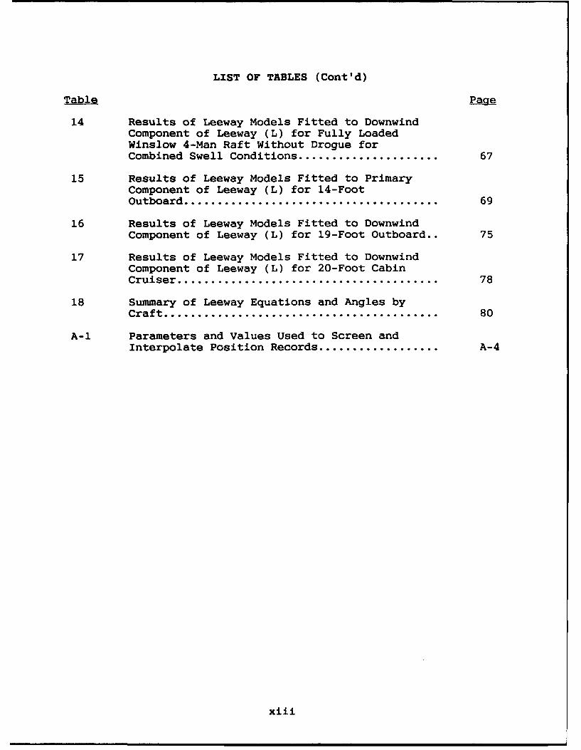
14 Results of Leeway Models Fitted to DownwindComponent of Leeway (L) for Fully LoadedWinslow 4-Man Raft Without Drogue forCombined Swell Conditions ..................... 67

15 Results of Leeway Models Fitted to PrimaryComponent of Leeway (L) for 14-FootOutboard ...................................... 69

16 Results of Leeway Models Fitted to DownwindComponent of Leeway (L) for 19-Foot Outboard.. 75

17 Results of Leeway Models Fitted to DownwindComponent of Leeway (L) for 20-Foot CabinCruiser ........................................... 78

18 Summary of Leeway Equations and Angles byCraft ............................................ 80

A-i Parameters and Values Used to Screen andInterpolate Position Records .................. A-4

xiii

IIIIIII

(THIS PAGE INTENTIONALLY LEFT BLANK]

IIIIIIUIIII

xiv

EXECUTIVE SUMMARY

INTRODUCTION

The Spring 1985 Leeway Experiment was a joint effort by the

U.S. Coast Guard Research and Development Center (R&DC) and

Florida Atlantic University (FAU). The experiment was conducted

off the east coast of Florida during March and April, 1985. This

report presents the results of the R&DC statistical analysis of

the data. FAU used the data to calibrate and test a numerical

leeway model. Their results are presented separately.

Leeway is defined as that movement of a craft through the

water caused by the wind acting on the exposed surface of the

craft. Leeway values of life rafts and small craft are needed in

order to predict the locations of survivors at sea. There are

seven classes of leeway targets in the current search planning

doctrine. A rule of thumb is provided for calculating leeway of

rafts with the addition of ballast buckets and a canopy; no

guidance is given for calculating the leeway of the newer deep-

draft ballasted type raft with drogue.

Four canopied life rafts and three small boats representing

the two broadest leeway classes and canopy/ballast bucket cases

were tested. A new category, the deep-draft ballasted raft with

drogue, was also represented. The life rafts were a Switlik

4-man raft, a Givens 6-man raft, an Avon 4-man raft, and a

Winslow 4-man raft. All but the Avon 4-man raft were deployed

with and without a drogue. The Switlik 4-man and the Givens

6-man rafts were circular canopied life rafts with deep-draft

ballast systems. The Avon 4-man raft was a circular canopied

raft with ballast bags. The Winslow 4-man raft was an oblong

canopied raft with no ballast system.

The three small boats were a 14-foot outboard, a 19-foot

outboard and a 20-foot cabin cruiser. The 14-foot outboard was a

flat-bottomed Boston Whaler-type outboard. The 19-foot outboard

was a sport fisherman with center console and outboard motor.

ES-1

i

The 20-foot cabin cruiser was a small, light-displacement cabin icruiser with two inboard-outboard motors.

The leeway of the small craft was determined by subtracting

the current of the upper three feet of the ocean from the test

craft's velocity. The current at the test craft was calculated

from an array of drifters surrounding the test craft. The

velocities of the drifters and the test craft were calculated

from their successive positions as determined by a Microwave

Tracking System (MTS). The wind was measured onboard the test

craft at a height of 6 feet.

RESULTS IDuring these tests a new class of leeway drift objects was

identified and tested. This new leeway class was canopied rafts 3with deep-draft ballast system and drogue. Both representatives

of this class were circular rafts. When drogued, these two rafts

were found to have zero or near-zero leeway for winds up to 13

knots.

Current leeway doctrine classifies the undrogued canopied

raft with the deep-draft ballast system as a light-displacement i

vessel with drogue. The Computer Assisted Search Planning (CASP)

system uses a range of leeway rates from 0.0335 to 0.0665. The

leeway rates of the Switlik 4-man and Givens 6-man rafts were

considerably lower than these and are presented below. This

confirms the results from the Summer 1983 Experiment that these

rafts drift more slowly than previously believed (Nash and

Willcox, 1985).

The raft with canopy and ballast buckets tested in this 3experiment was the Avon 4-man raft. Present leeway doctrine has

this raft drifting at the same rate as an unballasted raft i

without canopy, i.e., 7% of the wind (using the rules of thumb of

adding 20% for the canopy and subtracting 20% for the addition of 3

ES-2 3

ballast buckets). CASP uses a range of leeway rates from 0.0469

to 0.0931. Leeway speeds for the Avon 4-man raft from this

experiment were substantially lower than speeds calculated from

the leeway rates in CASP and are presented below. During the

Summer 1983 Experiment, the leeway of a 6-man raft of different

design, with fewer ballast bags and a different canopy style, was

found to be within present doctrine.

Data for the Winslow 4-man raft (canopy, no ballast) with

drogue are too limited for any firm conclusions. The leeway of

the Winslow 4-man raft without drogue was found to increase with

increasing wind speed and swell height. Using the rule of thumb

for adding a canopy, the leeway rates used by CASP would range

from 0.056 to 0.112. Leeway rates from this experiment for the

Winslow 4-man raft are lower than the rates used in CASP, they

are presented below.

The three small boats tested fit into the classification of

light displacement vessels. The leeway rates as used by CASP for

this classification are 0.0469 through 0.0931. Of the three

small craft, only the 14-foot outboard fell outside that range.

The 19-foot outboard and the 20-foot cabin cruiser drifted

downwind with their sterns to the wind. The 14-foot outboard

drifted beam to the wind and off the downwind direction by +140

to -24, ±100. This deflection off downwind was well within the

350 used under the present doctrine.

RECOMMENDATION FOR OPERATIONAL LEEWAY GUIDANCE

The proposed modifications to existing search planning

doctrine are presented in CASP format since CASP is used for most

predictions involving any significant amount of drift time.

Canopied rafts with deep-draft ballast system and drogue: For

wind speeds up to 13 knots, the leeway speed is negligible.

There are no data for winds above 13 knots. The maximum

ES-3

m

deflection left or right of downwind for these rafts with drogue

does not exceed 10*.

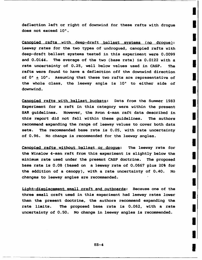
Canopied rafts with deep-draft ballast systems (no drogue):

Leeway rates for the two types of undrogued, canopied rafts with

deep-draft ballast systems tested in this experiment were 0.0099

and 0.0144. The average of the two (base rate) is 0.0122 with a

rate uncertainty of 0.25, well below values used in CASP. The mrafts were found to have a deflection off the downwind direction

of 00 + 100. Assuming that these two rafts are representative of 3the whole class, the leeway angle is 100 to either side of

downwind.

Canopied rafts with ballast buckets: Data from the Summer 1983

Experiment for a raft in this category were within the present

SAR guidelines. However, the Avon 4-man raft data described in

this report did not fall within these guidelines. The authors Irecommend expanding the range of leeway values to cover both data

sets. The recommended base rate is 0.05, with rate uncertainty 3of 0.96. No change is recommended for the leeway angles.

Canopied rafts without ballast or drogue: The leeway rate for

the Winslow 4-man raft from this experiment is slightly below the

minimum rate used under the present CASP doctrine. The proposed

base rate is 0.08 (based on a leeway rate of 0.0667 plus 20% for

the addition of a canopy), with a rate uncertainty of 0.40. No Ichanges to leeway angles are recommended.

Light-displacement small craft and outboards: Because one of the

three small craft used in this experiment had leeway rates lower

than the present doctrine, the authors recommend expanding the

rate limits. The proposed base rate is 0.062, with a rate

uncertainty of 0.50. No change in leeway angles is recommended.

I

ES-4 m

RECOMMENDATIONS FOR FUTURE RESEARCH

During this experiment, leeway was determined indirectly

from other parameters. New technology may provide a method of

measuring leeway directly without using a tracking system and the

number of personnel currently required. This new technology is

the electromagnetic current meter, which is capable of measuring

very low velocities and working in the wave zone. The new method

consists of equipping the test craft with both a wind instrument

and a current meter suspended under the craft. The current meter

would measure the motion of the craft through the water, i.e.;

leeway, directly.

The proposed method would require development of a suitable

instrument package to support a current meter and wind

instrument. If successful, the method would permit the

collection of leeway data without the constant maintenance of a

drifter array and tracking system. Leeway data for high wind

conditions could be collected by deploying a test craft before

the experiment begins and leaving it unattended. Tracking could

be accomplished either by satellite (Murphy and Allen, 1985) or

by a LORAN-C receiver and relay. (Allen, Eynon, Robe, 1987).

The collection of leeway data for higher winds and rougher

seas is needed to gain a better understanding of leeway.

Variations in leeway caused by the loading of a craft should be

determined. The maximum and minimum leeway values can be

determined by testing the craft fully loaded and empty.

The leeway of craft greater than twenty-five (25) feet in

length should be checked. The authors know of no successful work

in this area since 1960 (Chapline 1960).

The rafts referred to as canopied rafts with ballast

buckets need to be researched as a group. Regulations have

ES-5

I

required the addition of more ballast to this type of raft since Ithe early 1970's. Variations in ballast configurations for this

group could affect leeway. This class of rafts may constitute Ithe majority of the Coast Guard-approved rafts in use.

IIIIIIIIIIU

III

ES-6 3

CHAPTER 1

INTRODUCTION

1.1 SCOPE

The Spring 1985 Leeway Experiment was a joint experiment by

the U.S. Coast Guard Research and Development Center (R&DC) and

Florida Atlantic University (FAU). The experiment was conducted

in the Atlantic Ocean off Fort Pierce, Florida from 18 March to

16 April, 1985. The objective of the experiment was to increase

the accuracy of leeway rates used in drift predictions in search

and rescue. Leeway is defined as that movement, of a craft

through the water, caused by the wind acting on the exposed

surface of the craft.

The small craft used in this experiment (Table 1) were four

4- to 6-man canopied life rafts and three small craft from 14 to

20 feet in length. The rafts tested with and without drogues

were a 6-man circular life raft with a hemispheric ballast

system, a 4-man circular life raft with a toriodal ballast

system, and a 4-man oblong life raft with no ballast system. A

4-man circular life raft with ballast bags was tested without

drogue. The rafts were loaded to their rated capacity. The

small craft were tested without drogues.

This report presents the results of the R&DC's analysis of

the data. FAU has used the data to calibrate and test a

numerical leeway model and have presented their results

separately. R&DC participated in the experiment under element

1010.2.4, Improved Target Prediction, of the project "Improvement

of Probability of Detection in Search and Rescue," project number

1010.2. FAU's participation was funded under Grant DTRS 5683-

C00033, "On Drift Prediction", by the Office of University

Research, U.S. Department of Transportation.

III

Iw EQ co ( co c o IE-4 >4 >1 >

E, I>49

04-) 54 3

W 4 a4) ° 0 4 I: %3 4J r 4) r

4-) -H4.) 0) 0 4)4.o 4-) 4.4 4-) 3c 0f0 a -H w

% -.4 44 0 44 0 0 0i 0 M41 M04 (a 4.) CQ . 4-)

0444 O v 5 44 4J t4 w I

zI

E-40 0CM0*4> 4 0 0r0 V44 4.) ~ 4H - IV 4D15 rl 541

Q 04) 4) 0- 54) 04 00>4 w0 01 0CD 4 41 r. 41 04c.a1 H ) 4 40 w

DHW wW 0 H (0 (a 40

(0 0 4- 0 4-) Cd4Jr- 4-40) 0 HO

= H (al OH m o : C a 00 4- -

.4 IP 4 0C

544)

H H545 5

I44 (a toVH 0 0

>9 > 04P 4.J .U00 .01: I 10

H- to~.104 0 054. 44 0

Mv $D4 10 0 0 0 0IE- H H- 0 0 0

H 444 > 44 0 44 C 44 113 a - H0 V4 0 4'0 0

c125 p ~ w5 $4 V C1

2

1.2 BACKGROUND

1.2.1 Leeway in Search and Rescue

A key element of a successful search is the correct

prediction of the target location. For a search object located

on the surface of the water, the search planner must consider

some of the following sources of drift:

o Sea current,

o Wind-driven currents,

o Tidal currents,

o Miscellaneous currents from river runoff,

longshore currents, etc.,

o Wave- and swell-induced drift, and

o Leeway.

For the search planner, the components of leeway are leeway

speed and leeway angle. Leeway speed is the speed at which the

wind will push an object through the water. Leeway angle is the

angle off the downwind direction to which the object will sail.

The leeway information in the National Search and Rescue

Manual (SAR Manual) is presented in Table 2. The listed

references are believed to be the original studies on which the

equations are based. The SAR Manual does not list references.

Separate equations for winds above and below 5 knots are used.

For winds above 5 knots, the equations are an empirical fit of

data. For winds below 5 knots, there were insufficient data.

However, since there can be no leeway without wind, a straight

line was drawn from the origin to the leeway for 5 knots of wind.

The SAR Manual advises that the leeway speed for rafts in

Table 2 should be increased by 20% for the addition of a canopy

and decreased by 20% for the addition of ballast buckets.

3

us 0 0-t -a .60 060 0 0

09~ 0 - -: 1.0 - 41 4 4 4

u u4 41 1 -

-j

0 F" t" a 10 an*1 la+ 1 +1

mI

us' 3 3

us t.j

c -

o l 0a.. WIa a -

39I* a*

C2 4, C3 ja 0

*U- 41

N. *L

0 t1

B 0

CL 0 . U0

'A - au . a0.

4- - .. 0 CL 1

9L' C C-

a a

a 10 a; ON

.~ .:'3.-R.. '~ 4

The leeway information used by the Computer Assisted Search

Planning (CASP) system as of December 1985 is presented in Table

3. Leeway rate is the ratio of leeway speed to wind speed. T~e

base leeway rate is the estimated rate for a particular craft.

Rate uncertainty is a measure of the scatter in the leeway rate

data. A rate uncertainty of 0.33 means that the true leeway rate

is within + 33% of the base leeway rate.

TABLE 3

LEEWAY INFORMATION AVAILABLE IN CASP

Rate Leeway AngleTarget Description Base Leeway Rate Uncertainty (degrees)

Anchored on land(no drift) 0.00 0.00 00.0

Person in the water(zero leeway) 0.00 0.00 00.0

Light-displacementvessel withoutdrogue. 0.07 0.33 35.0

Large cabin cruiser 0.05 0.33 60.0

Light-displacementvessel with drogue 0.05 0.33 35.0

Medium-displacementsailboat/fishingvessel 0.04 0.33 60.0

Heavy-displacementdeep-draft sailingvessel 0.03 0.33 45.0

Surfboard 0.02 0.33 35.0

Using a Monte-Carlo simulation, CASP computes many replications

of a given target's drift using the base parameters (time,

position, current, wind and leeway characteristics) and the

uncertainty for each parameter. CASP permits the operator to

define leeway characteristics (base leeway rate, rate

5

I

uncertainty, and leeway angle). For any given replication, a n

leeway angle is randomly selected from a uniform distribution of

leeway angles ranging from the maximum leeway angle to the left Iof downwind to the maximum leeway angle to the right of downwind.

The replication's leeway rate is randomly selected from a uniform

distribution of leeway rates ranging from the base leeway rate

multiplied by (1.0 - rate uncertainty) to the base leeway rate

multiplad by (1.0 + rate uncertainty).

1.2.2 Previous Leeway Investigations I1. The Woods Hole Oceanographic Institution conducted a series Iof leeway drift studies from November 1943 through April 1944

using the Navy Mark I, II, IV, and VII and the Army A-3 and E-1

rafts (Pingree, 1944). These small I- to 5-man rafts were tested

loaded, with and without drogues. The tests were conducted in

three marine environments: Buzzards Bay, Massachusetts; off of

Boca Grande Island, Florida; and in the open ocean northeast of

the Bahama Islands. Pingree's (1944) drift results were

calculated using currents in the upper 15 feet of the ocean

(Figures 1 and 2). Note the considerable scatter at wind speeds

of 4 knots and less. I2. In 1959, a leeway study called "Operation Spindrift" was

conducted offshore of Hawaii using vessels and small craft from

the Coast Guard Auxiliary, local commercial fishermen, and other

willing boaters (Chapline, 1960). The drift due to currents was

removed by recording all positions relative to a 300-foot-long by

15-foot-wide fine mesh drift net. The observation vessel took

positions by radar ranges and visual bearing every half hour. INo mention was made of the use of drogues. Chapline (1960) used

a linear model passing through the origin for the analysis (Table

4). This model assumes that leeway is a constant percentage of

wind speed for a particular craft.

3. The Canadian Central Tactics and Trials Organization (CTTO),

6

Iw+D

3. 0 c

(0 x u +0 Z Lw w-

crci

+~ oiZ L LL c

Z'H w

Cc Mr (soW CLd

0i-Q 0 C0

wL -

(n ci

cii 3

__ __

.z -JL

L U

___ __ ciCw c Lr

0 .2

w10~

oow~

04,,

+. + cr r-

0:0

0so~ Octd (6NIM

+ <

II

TABLE 4LEEWAY RATES FOR MODERATE-TO-FRESH WINDS

(Chapline, 1960)

Group Craft Leeway Rate

I Surfboards 0.02

II Heavy-displacement, deep-draft sailing vessels 0.03

III Moderate-displacement, moderate-draft sailing vessels and fishing Ivessels such as trawlers, trollers,sampans, draggers, seiners, tunaboats, halibut boats, etc. 0.04

IV Moderate-displacement cruisers 0.05

V Light-displacement cruisers, out-boards, planing hull types, skiffs,etc. 0.06 I

working with the Canadian National Physics Laboratory (NPL),

conducted laboratory tests in late 1972 and early 1973 to

determine the leeway drift rates for several life rafts. Wind

drag was determined in wind tunnel testing, water drag was Idetermined in a tow tank, and wave-induced drift was measured in

a tank equipped with a wavemaker. The life rafts were l-, 5-, 9-,

and 26-man canopied life rafts with inflatable floors. Personnel

were simulated at 180 pounds per person. The report made no

mention of any type of ballast system on the rafts. The rafts

were tested with different degrees of loading, closed and open

doors, inflated and deflated floors, and undrogued and drogued

with two different types of drogues. Based on the wave tank

test, CTTO gave a wave-induced drift velocity of 0.6 to 1.0 knots

for fully developed seas due to winds in excess of 15 knots. IIn the CTTO report, leeway speed to wind speed was presented

for the different rafts in back-to-back logarithmic plots (not

reproduced here). This information has been generalized into

leeway rates by the raft's capacity and drogue employment (see

Table 5). The range of leeway rates results from variations in

8

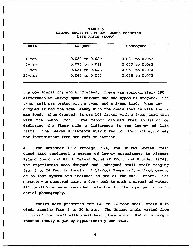
TABLE 5LEEWAY RATES FOR FULLY LOADED CANOPIED

LIFE RAFTS (CTTO)

Raft Drogued Undrogued

1-man 0.020 to 0.030 0.031 to 0.052

5-man 0.025 to 0.031 0.047 to 0.062

9-man 0.034 to 0.043 0.061 to 0.074

26-man 0.042 to 0.049 0.058 to 0.072

the configurations and wind speed. There was approximately 19%

difference in leeway speed between the two types of drogues. The

5-man raft was tested with a 5-man and a 2-man load. When un-

drogued it had the same leeway with the 2-man load as with the 5-

man load. When drogued, it was 10% faster with a 2-man load than

with the 5-man load. The report claimed that inflating or

deflating the floor made a difference in the leeway of life

rafts. The leeway difference attributed to floor inflation was

not inconsistent from one raft to another.

4. From November 1972 through 1974, the United States Coast

Guard R&DC conducted a series of leeway experiments in Fishers

Island Sound and Block Island Sound (Hufford and Broida, 1974).

The experiments used drogued and undrogued small craft ranging

from 9 to 24 feet in length. A 12-foot 7-man raft without canopy

or ballast system was included as one of the small craft. The

current was measured using a dye patch to mark a parcel of water.

All positions were recorded relative to the dye patch using

aerial photography.IResults were presented for 12- to 22-foot small craft with

winds ranging from 5 to 20 knots. The leeway angle varied from

50 to 600 for craft with small keel plane area. Use of a drogue

reduced leeway angle by approximately one half.

9

U

Leeway speed was not significantly different for the Idifferent craft, so all were combined into drogued and undrogued

categories. For undrogued craft, the leeway speed (L) was found

to be:

L = 0.04 + 0.07W, I

where W is the wind speed and both L and W are in knots. For Ismall craft with drogues, the relationship is I

L = -0.12 + 0.05 W, Iwhere L and W are in knots.

Hufford and Broida (1974) reported that an increase in seas from U2 feet to 4 feet resulted in an increase in leeway of

approximately 15%.

5. The U.S. Coast Guard Oceanographic Unit conducted a series 3of leeway experiments from January 1968 through March 1971

(Morgan, et al., 1977). The test craft were the MK7 life raft

without canopy, a 16-foot outboard motor boat, an 18-foot motor

launch, and a 30-foot utility boat with cabin. The MK7 life 3raft, a 7-man oblong raft without any ballast system, is

approximately 12 feet long. The current was measured by means of

a buoy with a 28-foot diameter parachute drogue. All positions Iwere determined by visual bearings and radar ranges from the

research vessel. The results in Figure 3 were determined by 3using a linear regression on 5-knot intervals of wind speed data. I

Morgan (1978) presented the results for the MK7 life raft

with drogue (sea anchor). The leeway rate for winds above 5 3knots was found to be "essentially constant at 0.04" with a range

of +0.03. The leeway angle was found to be 350 to the right for

a 5-knot wind and approximately 0* for wind speeds above 10

knots.

10

32 7 Mam30 *. Raft

I ~28267

24 I 16Boat -- w-On22- 0oa

20 (With Ouestionable Data)

18 -53 16CL 14cnO 12

~1O - /(Ithout Questionable Data)

8

* 2

0-

0 12

LEEWAY (knots)

I FIGURE 3. LEEWAY VERSUS WIND SPEED (Adapted From Morgan, 1977.The lines denoted as "R&D Center Equation" are from Hufford andBroida, 1974.)

I

6. The U.S. Coast Guard Oceanographic Unit, on a cruise aboard Ithe USCGC EVERGREEN (WAGO 295) from 15 February through 7 March

1978, conducted a leeway study for undrogued, canopied life rafts

(Scobie and Thompson, 1979). The current was measured by a buoy

equipped with a 10-foot square window-shade drogue. Results

were calculated for one 6-man, one 20-man, and one 25-man life

raft. All of these rafts had ballast systems. The rafts were

weighted with sand bags to represent passenger loading. For

winds of 10 to 35 knots and seas of 5 to 15 feet the leeway speed

was found to be: IL - 0.060 + 0.042 W

where L is leeway in knots and W is wind speed in knots. The

leeway angle was less than 300 for 78% of all drifts.

7. The U.S. Coast Guard R&DC combined leeway experiments with Iother experiments in January 1979, February 1980, and February

1981 (Osmer, et al., 1982). The first two experiments were n

conducted at sea with USCGC EVERGREEN. The current was measured

using a buoy with a window-shade drogue at a depth of 98 feet. 3Positions were determined from EVERGREEN using radar ranges and a

microwave ranging system or radar and visual bearings. The third n

experiment was conducted near shore using a Microwave Tracking

System (MTS) for positioning. The current was determined using

expendable surface current probes. The experiments used a

variety of 4- to 6-man life rafts with and without canopies and

drogues. Due to the considerable scatter in the data, no 3conclusions were reached. Osmer, et al. (1982), recommended that

the MTS be used in the shore-based mode for future leeway n

experiments. I8. In July 1982, the R&DC conducted a trial using the MTS to

track both the rafts and specially constructed drifters. The

drifters, designed to be tracked by the MTS, were used to

determine the current near the raft. In July and August

12 3

I

1983, a preliminary leeway experiment was conducted in Block

Island Sound using three circular, nearly empty, canopied rafts

without drogues (Nash and Willcox, 1985). The rafts were a 6-man

raft with two half-cylinder ballast bags (6-inch draft, RFD 6-

man), a 4-man raft with a toroidal ballast system (14-inch draft,

Switlik 4-man), and a 6-man raft with a hemispheric ballast

system (28-inch draft, Givens 6-man). The last two rafts were

deep-draft ballasted life rafts. Wind was measured at a small

boat anchored in the test area. Wind speed ranged from 2 to 11

knots, with waves of 0 to 2 feet and swells up to 4 feet.

The experiment was successful in differentiating the leeway

between the lightly and more heavily ballasted rafts (see Table

6). The leeway of the canopied raft with ballast bags was found

to be similar to the SAR Manual's recommendation for canopied

life rafts with ballast buckets. The leeway of the deep-draft

ballasted life rafts was much slower than the Scobie and Thompson

results.

TABLE 6LEEWAY SPEED FROM THE SUMMER 1983

R&DC EXPERIMENT

Life Raft Leeway SpeedCapacity Ballast System (Knots)

6-man Ballast bags 0.145 + 0.0568 W

4-man Toroidal 0.100 + 0.0083 W

6-man Hemispheric 0.100 + 0.0064 W

IThe leeway angle for the raft with ballast bags was found to

be highly dependent on the raft's orientation to the wind. The

circular deep-draft life rafts drifted downwind or very close to

I

1 13

m

downwind with no correlation between the leeway angle and the

raft's orientation to the wind. Nash and Willcox (1985)

recommended that all test craft be instrumented to measure wind 3speed, wind direction, and the craft's heading so that leeway

angles could be determined correctly. They concluded that much

of the reported variability in leeway angles was due to errors in

determining the wind and current.

IImI1IIImmmIU

14

CHAPTER 2

THE EXPERIMENT

2.1 DESIGN AND CONDUCT

Determination of leeway requires very accurate measurement

of the forces involved. The parameters that must be measured

accurately are the velocity of the test craft, the speed and

direction of the current, the wind at the test craft location,

and the height and direction of the waves. The craft's velocity

was determined using positions obtained by the MTS. The current

at the test craft was calculated from the position records of an

array of drifters (Figure 4) deployed around the test craft and

tracked by the MTS. The wind and the craft's orientation to the

wind were measured onboard the test craft. Wave height and

direction were recorded by the research vessels and by an

environmental buoy.

The monitor vessel (R/V OCEANEER IV) deployed two test craft

and surrounded them with the drifter array. As the test craft

drifted through the array, the R/V OCEANEER IV deployed

additional drifters to keep the test craft surrounded and also

recovered drifters no longer required for the array. The R/V

OCEANEER IV collected general environmental information every 20

minutes, operations permitting. An environmental buoy, moored in

the test area, collected wind, wave, and temperature data. When

FAU was on scene, the R/V BELLOWS took stations to collect any

additional environmental information required.

Test craft were paired according to their expected leeway

characteristics to isolate differences between craft types and

the effect of using drogues (see Table 7). This also minimized

the dispersion of the test craft so that the drifter array could

be maintained without either redeploying one of the test craft or

deploying a second drifter array.

15

II0U

9,. _9i1L.

211lw36" U

TO VEWSIDE VIEWI

24" rHandlesI

711"SIDE VIEW

FIGURE 4. MTS DRIFTER

161

4-)

CY) r- N1 %o to LO CV

'- 44r- 0 0 H C1 r4 H H 0 CN

z ()

:

4.)

C4 '-4 Hr U (C) 1

o o X ni fC:. 10 0 0* E- 0Y 0- 0 0% (7

04 w0 '0 L NNO

a)4 I C'4 C') N N-

H~~~U 0. o H H H>44 m 1 o ) )a

I3 0 I3 1 I 0I )0

.00 .0. . 14 43

04 0- Nr 41 - . H N 0 NH 0H

44 4-) 44a). 4 4. :4 :4

M 44 0 44) 0 0)0 4 N( 0wa coW O $.4 M U) 4 - $ J

H4-' 4r4 44. 4- 444O O10~~ 4. : ) 4.) qo 0 % w

4.(a a)) 4J) 4.T H J

4.4. 4.4a 4.4 4a.) 0 0 4044 04 04.c 4 C 14. r. 0 ~ 0 r.00-404 401 40 4) 4 4 4 0 -4. -4 A r.4 0 C:

.4 >4 >.4 >. 444>.4 4 .)4) 4 4.4 0 4c04

0H ff0 ff0 ffo f3 j (oH :3- >f - 2>V

0) u. 00 0. '0 0.V 1.' ff O

14 X X01.41 0117

i

The experiment was divided into three phases. Phase One (18 n

through 29 March 1985) consisted of the R&DC set up and

conducting drifts of the deep-draft life rafts with and without Idrogues. Phase Two (30 March through 7 April 1985) was the joint

part of the experiment. R&DC and FAU conducted drifts of small

boats and of deep-draft life rafts with and without drogues. The

environmental buoy was deployed in the middle of Phase Two.

During Phase Three (8 through 16 April 1985), the R&DC conducted

drifts of the lightly ballasted and unballasted rafts, and

secured the experiment.

Details of data collection are discussed in the following Isections.

2.1.1 Position IPositions of the deployed drifters, test craft, and research

vessels were determined every two minutes by an MTS. The MTS

consisted of a Motorola Falcon 492 tracking system controlled by

a Hewlett-Packard HP 9920 microcomputer. The MTS is made up of

three types of units: a master station whose position is known, Ireference stations whose positions are known, and mobile units

whose positions are to be determined. An example of the i

operating principle of the MTS is:

a. The master station transmits a coded signal containing

the identification codes of a particular mobile unit on frequency

A and to a reference station on frequency B.

b. A mobile unit, upon receipt of its identification code Uon frequency A, retransmits the signal back to the master station

on frequency C. n

I18i

c. A reference station, upon receipt of its identification

code on frequency B, retransmits the coded signal on frequency A

which is received by the mobile unit. The mobile unit then

retransmits a coded signal to the master station on frequency C

for the second time. This provides the master station with a

direct range to the mobile unit and a loop range from the master

station to the reference station to the mobile unit and back to

the master station.

d. The master station measures the time from the original

transmission to receipt of the signals on frequency C, calculates

the distance of the mobile unit from the master and reference

stations based on the two returned signals, the speed of the

transmitted signal, and the distance between the master station

and the reference station. The position of the mobile unit is

calculated using trigonometry and the positions of the master and

reference stations.

For each position determination, MTS repeaLs the above

sequence about 20 times and averages the results using filtering

and quality control checks. It can track up to 24 transponders

simultaneously and determine a round of positions every 30

seconds.

The MTS configuration during this experiment had the master

station (R&D Control) located on the roof of the Sea Palms

condominiums in Fort Pierce, FL. The northernmost of the two

reference stations was located in Vero Beach on the southernmost

tower of the Spires condominiums. The southern reference station

was located on the meteorological tower for the Florida Light and

Power Co. St. Lucie Nuclear Power Plant in Stuart, FL.

A survey error in the positions of the master and reference

stations degraded the absolute geographical accuracy of the MTS.

A position determined by the master station and one reference

19

I

s-t.ation was offset from the position as determined by the master

station and the other reference station. The relative accuracy

of the master and either reference station was not affected.

Essentially the MTS became two separate navigational grids, one

for each reference/master station pair. Alignment to true north

of each grid was checked by comparing directions determined using

LORAN-C. The directional error of the MTS grids was determined

to be 10 from true. The relative accuracy of the MTS positions

was ±30 meters for the same grid. For this study, relative

distances and directions are important. The lack of absolute

geographical accuracy prevents velocities from being calculated

between positions determined using the two different grids.

The MTS used the Florida State Plane Coordinate System in

meters in lieu of latitude and longitude. The coordinate plane

is a Cartesian coordinate system with the x and y axes increasing

to the east and north, respectively. The errors due to the

curvature of the earth are insignificant for the small test area;

therefore, the complexity of a spherical coordinate such as

latitude and longitude may be avoided.

2.1.2 Test Craft's Instrument Packages

The wind data on the test craft were collected using two

automated instrument systems each consisting of four components:

a propeller-type anemometer and wind vane, a flux-gate compass,

controlling circuits for the sensors, and a programmable

microprocessor-controlled data logger. One data logger had 32K iof internal memory, of which 15K was available for data storage.

The other had 64K of internal memory with 47K available for data

storage. The components of each package were interchangeable

with the corresponding components of the other package. Each

package was mounted on a plywood base with the wind sensor

mounted at a height of six feet. The accuracy of wind

measurements by these packages was +100 and +1.0 knot. The

I20n

threshold of the wind sensor was two knots. Wind data consisting

of 3-second averages were collected every 20 to 40 seconds

depending on the data logger used in the package. The data were

written out to a microcomputer at the end of each day.

Another wind instrument package used on the target test

craft was a Brooks and Gatehouse Hercules System 190. It is a

microprocessor-controlled instrument package designed primarily

for sailing yachts and ocean racing. It uses a flux-gate

compass, and a cup anemometer and wind vane. The wind sensor was

mounted at a height of six feet. The accuracy of the system as

mounted was approximately ±100 and +2 knots. One-minute averages

of the wind were recorded every 20 minutes by an FAU graduate

student onboard the test craft. This wind measurement system was

used only in fair weather.

2.1.3 R/V OCEANEER IV

U Environmental observations were recorded by the R/V OCEANEER

IV every 20 minutes when operations permitted. The environmental

observations consisted of wind speed and direction, height and

direction of the waves and swells, and a general description of

the weather (cloud cover, visibility, fronts, etc.). The wind

was measured with the R/V OCEANEER IV dead in the water using a

Brooks and Gatehouse wind sensor similar to the one described in

Section 2.1.2. The wind sensor was mounted at a height of

12 feet. This wind measurement was used only for a backup of the

wind meas red on the test craft. Swell and wave height were

estimated by eye. Swell and wave directions were estimated using

the R/V OCEANEER IV's magnetic compass. The R/V OCEANEER IV did

not record environmental observations when the R/V BELLOWS was on

* scene.

21

I

2.1.4 R/V BELLOWS I

During the joint R&DC and FAU part of the experiment, the

R/V BELLOWS occupied stations around the drifting array. At the

station locations the following measurements were taken: wind

speed and direction, height and direction of wind waves and

swells, currents, and a general description of the weather. The

stations were spread approximately two miles in the north/south

direction (along shelf) and one mile in the east/west direction

(across shelf). Time intervals between stations ranged from 10

to 25 minutes. Once a day, an expendable bathythermograph (XBT)

was used to determine sea temperature as a function of depth.

Wind was measured using a hand-held anemometer while the vessel

was dead in the water. The height of the wind measurements

ranged from approximately 12 to 25 feet depending on where on the

vessel the observer could get a clean exposure to the wind. This

wind measurement was used only as a backup for the wind

measurements made on the test craft. The heights of the swells

and waves were estimated. Swell and wave directions were

measured in reference to the R/V BELLOWS' compass. Current

measurements were made at depths of 3, 6, 9, and 12 feet using a

current meter with a deck readout.

2.1.5 Environmental Buoy

The environmental buoy was deployed from 3 through 15 April U1985 at position 27°33.24'N 80°05.91'W. Once an hour, the buoy

measured the wind, air and water temperature, and relative

humidity. The wind measurement consisted of a 10-minute vector

average and the maximum gust during that 10-minute interval. The

winds were measured at a height of 10 feet. The air temperature

and relative humidity were measured at a height of eight feet.

Water temperature was measured at a depth of three feet. Every

three hours, the buoy sampled a 1-dimensional wave spectrum

(height) for 20 minutes.

I22

2.2 DRIFTERS

The MTS drifters, designed and constructed at the R&DC,

consisted of a waterproof box between two 3-foot by 3-foot

plexiglass sheets; the waterproof box protrudes through the top

sheet (Figure 4). An MTS transponder with batteries was

contained in the waterproof box and was connected by a flexible

wave guides to an antenna on a pole which extended seven feet

above the upper sheet. The drifters float with the upper sheet

slightly submerged. A 40-pound lead weight suspended from a

four-point bridle attached to the four corners of the lower sheet

provides stability.

The MTS drifters were designed to have minimal leeway and to

measure only the surface water current that would affect a life

raft or a shallow draft vessel. This design was as effective as

drift cards in marking the upper layer of the water (see Nash and

Willcox, 1985). The drifters have an effective draft of nine

inches. The total draft is approximately three feet with the

counterweight. However, the surface area of the bridle and

counterweight is negligible when compared to the main body of the

drifter.I2.3 TEST CRAFT

I Leeway data were collected on four canopied life rafts and

three boats. The two circular life rafts with deep-draft ballast

systems were the Switlik 4-man and Givens 6-man rafts. Both

rafts were tested with and without drogues. The circular

canopied life raft with ballast bags was the Avon 4-man raft,

which was tested without drogue. The oblong canopied raft

without any ballast system was the Winslow 4-man raft. It was

tested with and without drogue. All rafts were loaded to

capacity using a simulated weight of 160 pounds per person.

23

II

The three small boats tested were a 14-foot Boston Whaler-

type outboard, a i9-foot center-console outboard, and a 20-foot Icabin cruiser. All three were tested without drogues.

2.3.1 Simulation of Life Raft Complement IFive-gallon water jugs filled with fresh water were used to

simulate survivors aboard the rafts. Water jugs were used

instead of the traditional sandbags to prevent overloading if theraft took on water. Some of the added weight caused by water

coming into the raft would be countered by the buoyancy of the Ipeople in the raft. Because sandbags do not float, a raft full

of water with 640 pounds of sandbags is much more heavily loaded

than the same raft full of water with 640 pounds (four 160-pound

individuals) of semi-floating people. Other advantages are that

a 5-gallon jug of water with a handle is much easier to load into

a raft in 3-foot seas than a bag of sand. In addition, water

jugs float when dropped over the side.

The jugs weighed approximately 40 pounds when filled; four

jugs were used for each person. The variation in weight of Iindividual jugs when filled was about 5 pounds. Therefore, a

person was simulated at a weight of 160 pounds, ±20 pounds.

Each raft was equipped with a wind instrument package that

weighed approximately 80 pounds. None of the rafts were deployed

equipped with survival gear; that gear generally weighs 10 to 20

pounds.

2.3.2 Switlik 4-Man Life Raft I

The Switlik 4-man raft was a circular raft with a toroidal

ballast system. The raft had a T-shaped canopy with the door

located at the head of the T (Figure 5). The ballast toroid was 3

i24i

divided into eight sections by baffles. Each section had a metal

bar at the bottom to aid in deploying and maintaining the bottom

shape of the system. A towing bridle (not shown in Figure 5) was

attached to the raft near the door and hangs down from the raft.

m When deployed with a drogue, the drogue was attached under

the canopy support tube opposite the door of the raft. A

parachute type of drogue was used; its diameter, when laid out

flat, was 31.5 inches. There were 8 lines, each 29 inches long.

The lines connected into a single point to which 50 feet of

parachute cord (550 pound test) was tied.

2.3.3 Givens Buoy 6-Man Life Raft

The Givens Buoy 6-man raft had a Y-shaped canopy and a

hemispheric ballast system (Figure 6). A towing bridle is

located on the side of the raft containing the door. This raft,

manufactured in 1983 for the R&DC, was modified by Mr. Givens

from the standard raft to include a deballasting slit in the bag

opposite the towing bridle. The slit was closed by lacing and by

sealing a flapper valve before deployment. The slit made

recovery of the raft easier and reduced the risk of damage to the

raft. The authors believe that the modification did not affect

the performance of the raft.

When the raft was drogued, a drogue identical to the drogue for

the Switlik 4-man raft (see Section 2.3.2) was used for the

purpose of this experiment only. The original drogue was

missing, and a replacement provided by Mr. Givens for this

experiment was of a type less common than the parachute-type

drogue. The same type drogue was used for both raft types to

emphasize the difference in raft designs. The exact drogue

carried by any brand of raft may vary as manufacturers or

repackers switch drogues.

25

60 2" 000

MR1 Ii I

DOOR

39"I

144

46'6' 2"

FIGURE 5. SWITLIK 4-MAN LIFE RAFT WITH TOROID BALLAST

26

Drogue

IRain PouchViwPr

Gas Cylinder

I 1o~:Gas Cylinder

I2L

Ballast Bag

Towing Bridle

FIGURE 6. GIVENS BUOY 6-MAN LIFE RAFT

* 27

I

When deployed, the drogue was attached with 80 feet of

parachute cord to the standard attachment point. This point is a Iwebbed loop on the bottom tube located directly under the canopy

support tube opposite the door of the raft.

2.3.4 Avon 4-Man Life Raft

The Avon 4-man raft has a canopy supported by a single tube

dividing the raft into two equal parts (Figure 7). The raft had

five ballast pockets (one larger than the others) distributed

around the bottom of the raft in a manner that is approximately Isymmetric to the line marked by the canopy support tube. The

raft was deployed without a drogue in this euperiment. This raft

was an older model and may not be representative of the rafts

currently made by Avon. The date of manufacture, serial number,

and any modifications are unknown. The ballast bags on the raft

do not match in size, shape, or location with drawings dated 1977

provided by Imtra Corporation, Medford, Massachusetts.

2.3.5 Winslow 4-Man Life Raft I

The Winslow 4-man life raft was an oblong raft with a canopy

supported by an arch at each end of the raft (Figure 8). It

lacked any type of ballast system and had only one base tube.

Although not approved by the Coast Guard, it is typical of the

rafts carried by many recreational and non-regulated vessels.

This raft used the soft carrying case as a drogue.

Unfortunately, the outer casing of the drogue line chafed through

during handling and parted when the drogue was deployed.

Therefore, the drogue from the Switlik 4-man raft (see Section

2.3.2 for description) was used. The drogue was attached to the

inflation pipes located on the base tube below the middle of the

door.

2

180R 26"

I -I i16-72"I.Ii j

( DOOR

16-

2

r'-,3"--i00r-l3-1045R

OO

I 16"

I 72"

S41" DOOR

DIAMETER

9", DIAMETER

FIGURE 7. AVON 4-MAN LIFE RAFT

29

II

2.3.6 14-Foot Outboard

This vessel was a 14-foot Boston Whaler-type outboard with

less than 6 inches of draft. It was equipped with a 25-

horsepower outboard motor that was kept in the down position

during the test. It was loaded with approximately 80 to 100

pounds of wind instrumentation and a 25-pound anchor. The boat

should be considered either lightly loaded or empty.

2.3.7 19-Foot Outboard

This vessel was a 19-foot center-console sport fisherman

with an outboard motor. This test craft always held one or two

persons and was fully equipped, including fishing gear. The

engine was always in the down position. The load on this vessel

should be considered normally loaded.

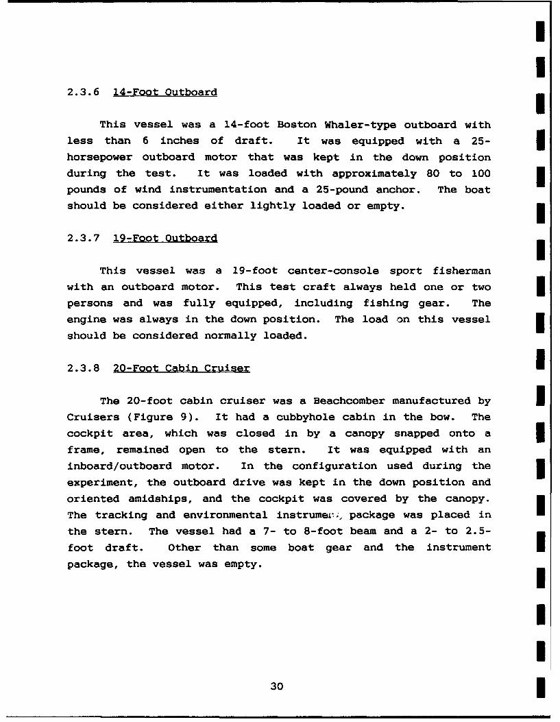
2.3.8 20-Foot Cabin Cruiser I

The 20-foot cabin cruiser was a Beachcomber manufactured by ICruisers (Figure 9). It had a cubbyhole cabin in the bow. The

cockpit area, which was closed in by a canopy snapped onto a

frame, remained open to the stern. It was equipped with an

inboard/outboard motor. In the configuration used during the

experiment, the outboard drive was kept in the down position and

oriented amidships, and the cockpit was covered by the canopy.

The tracking and environmental instrume-, package was placed in

the stern. The vessel had a 7- to 8-foot beam and a 2- to 2.5-

foot draft. Other than some boat gear and the instrument Ipackage, the vessel was empty.

II

30

-Canopy

SupportTubes

12"

I TOP VIEW

Drogue

I3 5,

* END VIEW

FIGURE 8. WINSLOW 4-MAN LIFE RAFT

* 31

I

IIIIIIIIIIIIII

Figure 9. Photographs of 20-foot cabin cruiserI

32

CHAPTER 3

DATA PROCESSING

3.1 INTRODUCTION

This chapter outlines the data inputs, the data processing

methods used, and the results obtained. The details are

presented in Appendix A.

The raw data included:

a. Position data for drifters,

b. Position deta for test craft,

c. Output from environmental instruments, and

d. Craft code and configuration information.

3.2 CALCULATION OF CURRENTS, TEST CRAFT VELOCITIES, AND LEEWAY

Position data from drifters and test craft were edited to

include only those positions when the platforms were drifting

freely and when positions were all provided by a single MTS

reference station. (Reasons for using a single reference station

are given in Section 2.1.1) A piecewise linear regression method

was used to eliminate questionable data points and to interpolate

for position data between known positions. Interpolated platform

position records for 4-minute intervals were created.

Current velocity components for each drifter were calculated

from the drifter position record by using a time-centered finite

difference algorithm. Currents for each drifter were combined

using regression equations to produce a current field in the area

of the test craft. The current at the test craft was obtained by

entering the craft's position into the regression equations.

33

U

Test craft velocities were calculated from craft position Idata using the same time-centered finite difference algorithm

used to calculate the current components at the drifters. ISubtracting the current at the test craft from the craft's

velocity yielded leeway speed and direction.

3.3 WIND DATA

Wind data collected onboard the test craft were used in the

leeway calculations. Automated instrument packages, used on all

test craft except the 19-foot outboard, provided analog voltages

from the compass, wind vane, and anemometer. Initial processing Iincluded changing analog readings to engineering units, computing

wind direction in degrees true, and compensating for differences

in instrument orientation.

Wind data from the automated instrument packages were

checked and edited to remove erroneous data points, to correct

for passage of the wind direction through the discontinuity at

3600/000 °, and to compensate for an offset caused by an equipment

problem. Average values for compass heading, relative wind Idirection (RWD), and wind velocity were determined; these values

were used to create 4-minute averages that corresponded in time

to drifter position records. (Relative wind direction is the

direction from which the wind blows, measured in degrees

clockwise about some chosen axis on the test platform.)

The Hercules 190 wind station, used aboard the 19-foot Ioutboard, provided 1-minute averages (recorded every 20 minutes)

for compass heading, wind direction in degrees magnetic, and wind Ispeed. Relative wind direction was computed, and wind direction

was converted to degrees true. A wind record for every minute

was created by assigning the nearest values in time to each

minute.

I

3.4 DATA COLLATION

Records for each day for a single craft were tabulated. The

records included the code for the craft, the date and time of the

individual data points, the craft's configuration (weight of

water jugs, deployment of drogue, engine in up or down position,

etc.), leeway speed and direction, wind direction, wind speed,

relative wind direction, compass heading, and number of drifters

used in current calculations.

3.5 LEEWAY ANGLE

Subtracting the wind direction from the leeway direction

* yields leeway angle; leeway angles are chosen to be positive for

deflection to the right of downwind and negative for deflection

* to the left of downwind.

3IIIIIIIII 35

IIIIII

[THIS PAGE INTENTIONALLY LEFT BLANK] I

UIIIIIIIIiI

36

CHAPTER 4

ANALYSIS

4.1 INTRODUCTION

* The objective of this analysis is to quantify the

relationship between leeway and wind for the craft tested.

Specifically, the following questions are considered:

1. How does the drifting craft orient itself to the wind?

2. Does the craft drift directly downwind or at some angle

to the wind? Is the angle unique?

* 3. What is the relationship between wind speed and the

craft's speed?

I The parameters that provide answers to these questions

include relative wind direction (RWD), leeway angle, leeway speed

I and leeway rate.

4.1.1 Significance of Parameters

1. Relative wind direction (RWD) is the direction from which

the wind blows, measured in degrees clockwise about some chosen

axis and point on the test craft. The convention for ships is to

measure from the fore-and-aft line using the bow as a reference

point. RWD quantifies the orientation of the craft to the wind

and permits differences in leeway attributable to orientation to

be identified. A rough example of how the craft's orientation to

* the wind is related to leeway angle can be seen in Figure 10. A

RWD of 225°R results in a negative leeway angle (to the left of

downwind), a RWD of 135°R results in a positive leeway angle (to

the right of downwind).

37

Wind To Wind To L E A

DIRECTIONLA LA

RWD u.225*R

RWD=-135"R

w-U

Wind WWindDirection Dieto

From DFrom

FIUR1. EATO O ELTIEWIDDIETIN7RDAND LEWAYANGL (LA38

The distribution of RWDs also indicates whether the craft

drift is influenced by the wind. If the craft is bouncing in the

waves and unaffected by the wind, the RWDs will vary considerably

as either the wind direction or the craft's heading changes.

Variation in RWD will decrease as the craft's response to the

wind increases. Thus, RWD can help identify the threshold value

* of wind speed needed to affect the craft's orientation.

2. Leeway angle is defined as leeway direction minus wind

direction, with a deflection to the right of downwind being

positive. The leeway angle parameter combines wind direction and

leeway direction. A leeway angle of 0° indicates that the craft

drifts directly downwind. Positive or negative values quantify

how far to the right or left of downwind the craft is drifting.

Realistic values of leeway angle are bounded by -90° and +900 for

measurable leeway speeds. Leeway angles for very low wind

speeds may exceed those bounds due to the measured leeway being

less than the measurement errors. Leeway angle estimates are no

better than the wind measurements, which were good to +10

degrees.

3. Leeway speed is the magnitude of the leeway velocity.

Most of the analysis will use the leeway velocity separated into

orthogonal components oriented parallel and perpendicular to the

downwind direction. Leeway speed cannot be less than zero;

however, leeway components may lead to negative values for

downwind leeway speed. Coefficients of leeway models determined

using leeway speed instead of the leeway speed components will

result in higher estimates of predicted leeway drift for a given

I wind speed.

4. Leeway rate is defined as the leeway speed divided by the

wind speed.

39

I

4.1.2 Leeway Models UThree leeway models (regression equations of leeway speed as I

a function of wind speed) were considered in this analysis to

quantify the relationship of craft speed to wind speed. The

models are:

L - b*W Equation 4-1 UL - a+b*W Equation 4-2

L - d*Wc Equation 4-3

where: L is the leeway speed,

W is the wind speed, and

a, b, c, and d are regression coefficients.

Equations 4-1 and 4-2 are standard leeway equations used in

previous studies and currently in use in search planning. The

third equation, known as a power curve, is a departure from the

assumption of a linear relationship between leeway speed and wind

speed. In some cases, the non-linear model produced the result

that the leeway rate increased as the wind speed increased, which

is not reasonable. In other cases, the non-linear model produced

reasonable results that were not sufficiently better than the

results of the linear models to justify the increased complexity.

Only the results of the linear models are reported here.

Methods of fitting the linear models to the data and the

error analysis are described in Appendix B.

4.2 SWITLIK 4-MAN LIFE RAFT

4.2.1 Switlik 4-Man Raft With Drogue

Data for the Switlik 4-man raft with drogue consist of 328

data points collected over 4.5 days. Wind speed ranged from 2.5

to 13.6 knots. Sea conditions ran from calm to 2.5-foot waves

40 I

I and 3-foot swells. There was considerable overlap of

environmental conditions from day to day.

The drogue was attached to the main bottom tube at a point

I located just below the canopy support tube opposite the door

(Figure 11). For this discussion, the convention for relative

bearings will be that the door is at the bow (000°R) and the

point of attachment of the drogue to the raft is at 1800R.

The RWD data show considerable scatter for wind speeds under

8 knots; however, the scatter in the RWDs is much less for winds3 greater than 8 knots (Figure 12). As the force of the wind on

the Switlik 4-man raft increases, the Switlik 4-man raft

increases its pull on the drogue. The increasing strain on the

drogue line holds its point of attachment to the raft into the

wind; however, the Switlik 4-man raft without drogue will never

have that canopy support tube (180 ° ) up wind (Nash and Willcox,

1985). The strain on the drogue line holds the raft in that

position when the wind speed increases to about 6 knots (Figure

13a and 13b). The bottom line of Figure 13a is the RWD plotted

using the left-hand scale; the top line is the wind direction in

degrees true plotted using the right-hand scale. The wind speed

(Figure 13b) dropped below 5 knots early in the drift, increased

to over 6 knots, and then dropped steadily to below 3 knots.

When the wind speed increased to 6 knots, the RWD approached

180°R (Figure 13a) where it stayed as long as the wind was

6 knots or greater. When the wind speed decreased below 5 knots

toward the end of the experiment, the RWD no longer held at

180°R.

The Switlik 4-man raft, when drogued, has no measurable

leeway movement for winds under 12 knots (Figure 14). Leeway

speed does not vary with increased wind speed and the values of

* leeway speed are low and scattered around zero leeway speed

(Figure 14). This data base does not permit extrapolation for

winds above 12 knots.

41

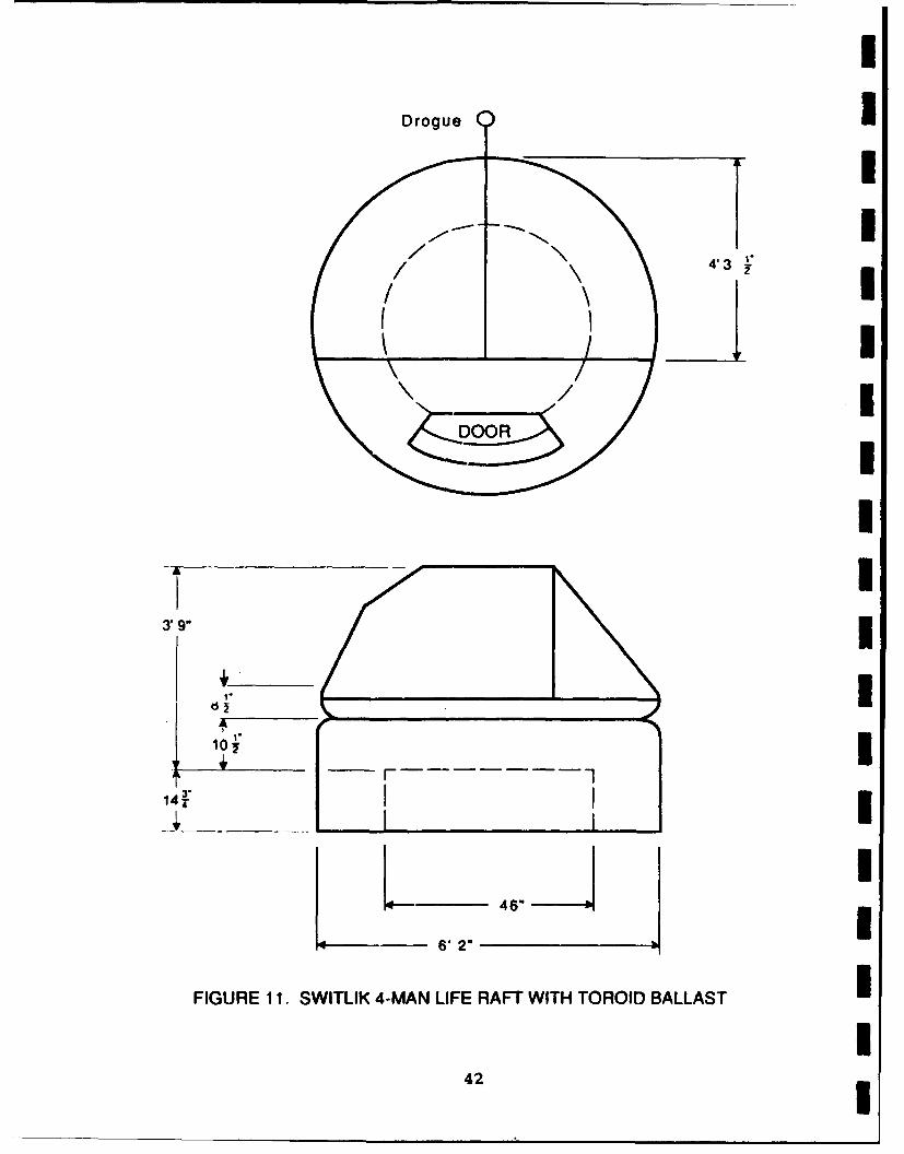
IDrogue()I

3"9"

fI

3'9"I

l " II o lOI

1o_ * __ I14274

6'2"

FIGURE 11. SWITLIK 4-MAN LIFE RAFT WITH TOROID BALLAST I

I42

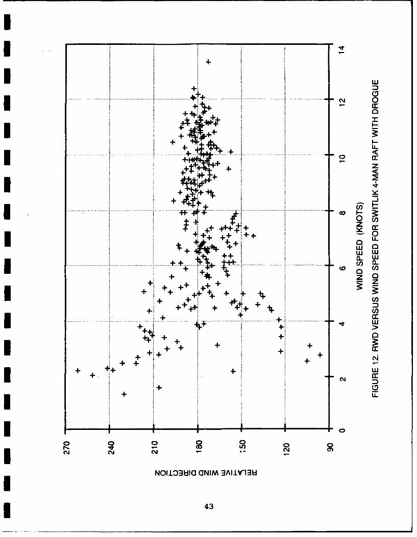
IL

i + ++ ++ 'i + -

ID

.. .. .. .. .. .. .. .. ... .. .. ..... ...... ..................+ ........ ............ ... ..... ........ .... ........... ............ .0

+

+.,. 3+ C

I ,-+. _..

++ <.

+0

I.. ...... ....

I 0_

...IJ.

!z

+ +o+ ++ ++ :*++- 0

+0+ W

. + +'r a)0.

-z,+ ++:++ I +~: + +i+ : §

++

+ ++0++ +

+~~ ++cI + ++ + +++3 + 0

* + .+L+

I k +

I 43

a) 270 -015

240 ---------- . . . .. ..+ .. ........... ......... . ......... ...... ...... !8

90 195

120 ........ .......... .... ... . . . . . ..............................

2 -

13.5 14.5 15.5 16.5

Hour of Day

b)UE1.DT F6ARL18 ORSILK4MNRF IHDOU

64

wc~Q.

.. .......... ..* ........ .... .. ... ...

.......... ............................. ............... .a

.. . ... . . . ... . . .. .. ... ........... .... . 4.

4 .:, zn+ ED 4.

z ~LL.. .. 4..... .. ... . ...

a. 4.Z#. Cl 0.

*~ M.

+ 45

I

4.2.2 Switlik 4-Man Raft Without Drogue IThe data base for the Switlik 4-man raft without drogue I

consists of 113 data points collected over 1.5 days. There is

almost no overlap of environmental conditions from one day to the

next day. One day had winds of 4.7 to 8.0 knots, waves of 1 foot

or less, and swells of 1 to 2 feet. The other day had winds of

8.7 to 13.6 knots, waves of 2 to 3 feet, and swells of 2 to 6

feet.

The RWD stayed in two sectors, 080°R to 120°R and 215°R to

225°R. The RWD of 180°R observed when the Switlik 4-man raft was Idrogued was never observed when the raft did not have a drogue.

The RWD changed sectors three times during the longest drift.

This is similar to the behavior noticed in the Summer 1983

Experiment (Nash and Willcox, 1985). RWD was found to have no

correlation to the leeway angle or to any component of leeway.

The crosswind component of leeway was less than 0.1 knots to m

the right and left of downwind. The crosswind component was not

correlated with wind speed. This confirms the conclusion from m

the Summer 1983 Experiment that the Switlik 4-man raft drifts

downwind (Nash and Willcox, 1985).

The downwind component of leeway (L) is presented in Figure

15. Small negative values of leeway speed at wind speeds of

5 knots represent variations in the data due to measurement

errors. The leeway models discussed in Section 4.1 and Appendix B

were fitted to these data (see Table 8). The standard error of

the slope is presented so that confidence limits can be obtained.The standard error of the estimate is indicative of the scatter

of the data around the regression line. The percent variance

explained is the percentage of the total variance, in the

downwind data leeway component, that is attributable to wind

speed. This percent variance is the coefficient of determination

multiplied by 100.

46

w

4 + U)_

+ 3:0

+ +

4.+

I,+ +

+ 0 L0

S-....-

0 LL

w a

i+ +

+ i i 0

+ -Z

C~~0 0

.... . (.. .. ..................... .... .......................

IL.........I. ........... ........... 4.......................

i

TABLE 8 IRESULTS OF LEEWAY MODELS FITTED TO DOWNWIND

COMPONENT OF LEEWAY (L) FOR SWITLIK 4-MAN RAFT WITHOUT DROGUE(Values for L are in knots. W is wind speed in knots.)

Model Standard Error of: % VarianceSlope Estimate Explained

L - 0.0144W 0.00036 0.03581 58

L - -0.0393 + 0.0183W 0.00139 0.03466 61

IBoth models provide similar answers over the data range. The

negative values produced by the second (L=a+b*W) at wind speeds

under 2 knots make it less realistic. Therefore, the first model

(L = b*W) is recomended.

The leeway equation derived during the Summer 1983 Experiment

was L - 0.100 + 0.0083W, where L (leeway) and W (wind) are in

knots. That equation was for a virtually empty raft and was

derived using the total leeway speed instead of the downwind icomponent. Therefore, one would expect higher leeway values for

that equation. For 3 knots of wind, the leeway speed using the

equation L - 0.100 + 0.0083W is 0.08 knots higher than a leeway

calculated using the new equation of L - 0.0144W. The difference

between the two equations decreases as the wind speed increases,

until eventually the new equation provides a higher leeway speed

than the 1983 equation. This crossover will take place at a wind

speed higher than the data range found during these experiments.

Both equations have the Switlik 4-man raft with slower leeway at

wind speeds above 6 knots than the equation L = -0.12 + 0.05W

given by Scobie and Thompson (1979).

4.3 GIVENS 6-MAN LIFE RAFT

4.3.1 Givens 6-Man Raft With Drogue

The data base for the Givens 6-man raft with drogue includes

48

142 data points collected over 1.5 days. Wind speed ranged from

2.3 to 13.5 knots with waves and swells of 1 foot or less. The

wind speeds on the half day of drift fell within the wind range

for the full day of drift.

The drogue was attached to the main bottom tube at a point

located just below the canopy support tube opposite the door

(Figure 16). For this discussion, the convention for relative

bearings will be that the door is at the bow (000°R), and the

point of attachment of the drogue to the raft is at 180 0 R.

The RWD data show considerable scatter for wind speeds under

8 knots; however, the scatter in the RWDs is much less for winds

greater than 8 knots (Figure 17). The raft appears to drift with

the stern (and the point of attachment of the drogue) nearly

toward the wind (170°R) when wind speeds exceed 8 knots. This

result is similar to results for the Switlik 4-man raft with

drogue (Section 4.2.1).

The downwind component of leeway is essentially zero for wind

3 speeds up to 13 knots (Figure 18). The Givens 6-man raft, when

drogued, has no measurable leeway movement for winds up to 13

knots. This data base does not permit extrapolation to winds

above 13 knots.

4.3.2 Givens 6-Man Raft Without Drogue

I The data base for the Givens 6-man raft without drogue has

sizable, with 320 data points collected over 4.5 days. Wind

speed ranged from 1.4 to 13.6 knots. Sea conditions ranged from

calm to 2.5-foot waves and to 3-foot swells. There was

considerable overlap of environmental conditions from day to day;

no one day had unique conditions.

49

I

180"R

Rain Pouch View Port

60OR D 1 300°RGas Cylinder I

~~7' 3" *

I31' DOOR

10 L_ Gas Cylinder I102 ! I

Ballast Bag I

Towing Bridle I

I

FIGURE 16. GIVENS BUOY 6-MAN LIFE RAFT

50 I

230-

220-.

4"

200-4

190 .......

o 180 . ............ 44...

4 4 40Cr 170-:4+ 484

160 .4........W 7.....

150'

140-

2.0 4.0 6.0 8.0 10.0 12.0 14.0

WIND SPEED (KNOTS)

I FIGURE 17. RWD VS WIND SPEED FOR 6-MAN RAFT WITH DROGUE

I5

wIwI

4 . ........... + ... ..... ..........+ + D

+ +4D

*L 04j+

.. .. . ... .. 0.... .. ... .

:4+ + IcWL...... ........ *. .... . + . ....... ... W - I

+4

+w w

+, >+~

I 1 + 0.*,o

*1 4 LL

J zoVI

........... : 1 ............... ................... ....... I- co

... .. ... .. .. .. .. . . . .. ... .. .. .. .

............ ..a...-...- . .....-

cm cm a D

(sIoNA) AVM99-1

52

The discussion of RWD will use the convention that the door

of the raft is located at 000°R and the canopy support tubes arelocated at 060°R, 180°R, and 300°R (Figure 16). The RWDs were

predominantly in three sectors: 340°R to 020*R, 090°R to 1300R,

and 230°R to 2700R. These sectors correspond to the areas

between the canopy support tubes. RWD changed sectors from one

to three times a day for winds greater than 6 knots. For winds

of 6 knots or less, the RWD varied with the wind direction. Anexample of the variation of the RWD with wind speed and direction

I can be seen in Figure 19.

The top line of Figure 19a is the wind direction "to" in

degrees true using the right-hand scale. The bottom line of

Figure 19a is the RWD using the left-hand scale. Figure 19b is

the wind speed in knots.

The horizontal axis is the hour of the day for 24 March 1985.

The change in the RWD record when the wind speed increases above

6 knots is striking. At wind speeds above 6 knots, RWD becomes

very steady at 240°R to 260°R (Figures 19a and 19b). This

* suggests that the raft is not strongly affected by winds under 6

knots.

The sector affected by the RWD had no effect on the

components of leeway or the leeway angle. There was no

correlation between the crosswind component of leeway and thewind speed. The raft drifts nearly directly downwind.

The downwind component of leeway (L) is presented in

Figure 20. The negative values around 5.2 knots and the positive

values for winds less than 5.2 knots are from two different days.

* Additional data would be needed to define the leeway for wind

speeds less than 5 knots.

53

a)

40 -- -310

. .... ... ... . ....20~

2 0 ....... .. ... .. ... ... .. .......... ............. ............ ............................ ----- ------

05... . ... ....... ....... ....... . ........ ....... ....... 3

3 4 . . . ... . . .. .. . .. . .. ..... ... .. ......... .... ...... .......... I-... .....

2 6 0 - . .....-.... I ... .......... ..................... ........

220 i Ii- -011.3 12.3 13.3 14.3 15.3

Hour of Day

b) 1.0 - - -------- - -

.. . . .. . .. .. .. .. . .. . .. . . . . .. . . . .. . . .. .. .. . . . . .. .. . . .. . .

80- ..... II I

0.

114.- 1231.I431.

Hour f DaF20.......U............. DAT OF2-.C 95FO IES6 NRATWTOTDOU

I j i 54

III

1 .20 *

I i I:i ~~.1 6 .......................... ........................ ..................... .. .......................... ................ ; i.......... ....... ... ...... ...... ..

.16 + + + + +'

0 . . -

1 2 . ......... ... • ..... ........ .., ......................... i ............ .... +-- ..... ... .. .. - ---- } ------ - --- ------ -- -..............

*W .04-!t 4 i,,, I! Tyv."'*.i.., :S!...t;4 I , t I' " i

+ + .

+

+

S+ I + I- 0.00 . .. ............................. . .................................................................

2 I0.00 . ..... ................ ........................m ....... ........ "-+ I.... ........ .... . . ................ . .. .. .. .... ..'

I 41 I

-.04 I-I -II

0.0 2.0 40 6.0 8.0 10.0 12.0 14.0

WIND SPEED (knots)IFIGURE 20. DOWNWIND COMPONENT OF LEEWAY VERSUS WIND SPEED

FOR GIVENS 6-MAN RAFT WITHOUT DROGUE

55

I

The leeway models discussed in Section 4.1 and Appendix B Iwere fitted to the Givens raft data (Table 9). Both models

explained 52% of the variance in the data set. The model

L = a + b*W has a value of (a) that is negligible. The first

model, L - b*W, is chosen for this data set.

TABLE 9

RESULTS OF LEEWAY MODELS FITTED TO DOWNWINDCOMPONENT OF LEEWAY (L) FOR GIVENS 6-MAN RAFT WITHOUT DROGUE

(Values for L are in knots. W is wind speed in knots.)

Model Standard Error of: % Variance ISlope Estimate Explained

L = 0.0099W 0.00015 0.02337 52 1L - - 0.0023 + 0.0102W 0.00055 0.02338 52 INo correlation was found between the downwind component of leeway

rate and wind speed, thus confirming the linear nature of the

leeway model.

The leeway equation from the Summer 1983 Experiment was

L = 0.100 + 0.0064W, where L (leeway) and W (wind speed) are in

knots. That equation was for a virtually empty raft and was

derived using the total leeway speed instead of the downwind

component. Therefore, one would expect higher leeway values for

that equation. In fact, for 3 knots of wind, that equation is

0.1 knots higher than the new equation of L = 0.0099W. The

difference between the two equations decreases as the wind speed

increases, until eventually the new equation provides a higher

leeway speed than the old. However, this happens at a wind speed

of 28 knots, which is well beyond the range of the data. When

wind speeds exceed 6 knots, both experiments have the Givens 6-

man raft with much slower leeway than the equation L = -0.12 +

0.05W (Scobie and Thompson, 1979).

I56 3

4.4 AVON 4-MAN LIFE RAFT

The Avon 4-man raft was tested without a drogue; 127 data

points were collected over 3 days. There was considerable

variation in the swell conditions; most of the data were

collected with either no swells or 4- to 5-foot swells (Table

10). The swells were traveling downwind within approximately 300

of the downwind direction.

I TABLE 10

ENVIRONMENTAL CONDITIONS REPRESENTED IN DATA FOR AVON4-MAN RAFT

Number of Date Wind Speed Waves SwellsPoints (feet) (feet)

75 8 April 1985 3.9 to 13.6 knots 0.5 to 2 0

48 10 April 1985 9.1 to 14.2 knots 2 4 to 5

4 14 April 1985 3.9 to 6.6 knots 1 2 to 3

The convention for RWD is that the center of the door is at000R, and the 045°R to 225°R line runs along the canopy support

tube (Figure 21). There are two distinct patterns for RWD data

for wind speeds greater than 8 knots (Figure 22). The first

pattern of RWD, starting around 165°R for 10 knots of wind and

decreasing to 125°R for 14 knots of wind, was for swells of 4 to

5 feet. The second pattern from the upper left-hand corner of

*the plot to the lower right-hand corner consists mostly of data

from 8 April 1985 (i.e., no swells).

I The RWDs of 0806R and 135°R may have some significance with

respect to swell or no swell at the higher wind speeds. Looking

back at Figure 21, an RWD of 135°R corresponds to a line

perpendicular to the canopy support tube and running through a

ballast bag. An RWD of 080°R also corresponds to a line drawn

from the center of the raft through a ballast bag. A silhouette

of the raft viewed from 135 ° would be greater than one viewed

57

1 80R 26" I'

I I- 16-

16-2

r- 1045R 45RUO

16"

4 72"-

__ __ _r- 2 4 -- l

41" DOORI

80 1 4DOIDIAMETER

FIGURE 21. AVON 4-MAN LIFE RAFT

58

F 4

... ....V

441+i+ i... .. ? , .. 0

+1 + - I

.. ~1 . ... .. ..... ..

4.. - I...... ..... Hr

+ z

~+ 41. U

4 1 o 0

. . . . . . .......... 0...... ........... .... .... .. ....

+ wW m

c.C',

* 0

.l in tn kn Lnt nCY 0 w cm0 co

..................................... V.

N0119HIOGNIM3AI-V13

59. ,

I

from 0800R. The area of the silhouette corresponds to the sail Iarea available for the wind to push. Thus, a wind from 135 0R

would exert a greater force on the raft than the same wind from

080 0R.

The presence of swell appeared to affect the raft's 1orientation to the wind. Differences in orientation might

produce differences in leeway. The effects of swell and raft

orientation cannot be separated in this data set. The data were

combined for analysis.

The downwind component of leeway (L) for the Avon 4-man raft

without drogue is presented in Figure 23. Leeway models

discussed in Section 4.1.2 and Appendix B were fitted to these

data (Table 11). The second model (L = a+b*W) provides the best

fit to the data.

4.4.1 Summary for Avon 4-Man Raft

The Avon 4-man raft exhibits at least two patterns of

orientation to the wind.

TABLE 11

RESULTS OF LEEWAY MODELS FITTED TO DOWNWIND COMPONENT OF LEEWAY(L) FOR AVON 4-MAN RAFT WITHOUT DROGUE

(Values for L are in knots. W is wind speed in knots.)

Model Standard Error of: % Variance ISlope Estimate Explained I

L - 0.0081W 0.00055 0.06508 51

L - -0.1412 + 0.0213W 0.00217 0.05704 66

I

60 I

II.

~LOI r 0

++,. .. ........... ... .V.. ..)+ V- zI LULU

+ +

I "4 ,C (1 jlI+ z

I .. Cl

I 4 + >4 + + + ~

I+ + 44

e"+U

* 4 4 T-,+ 4'

. . .. . . .+ 0 <

I*(ION )C33:1 WI-3

I- LL Ur

I~ 0

Y 0zw z~

0 Z0IC 00

0

CMJ

-o LL

0 0 0C~j 0 0) 00i 0i 6i 6

(SIoNA) 033dS AVM33J1

* 61

I

Leeway speeds calculated using the Avon 4-man raft model from Ithis experiment are consistently and substantially lower than

leeway speeds calculated using the CASP leeway rate of 0.07.

Because of the high negative leeway values predicted at low wind

speeds and the high variability of leeway angle the results are 3questionable.

The CASP leeway rate of 0.07 represented the class of raft Kused in the Summer 1983 Experiment (Nash and Willcox, 1985)

fairly well; howeve-, the Avon 4-man raft has more ballast (more

and larger bags) and is smaller than the 6-man raft used in the

Summer 1983 Experiment. The results suggest that the class

description "raft with canopy and ballast bags" is too broad a

classification.

4.5 WINSLOW 4-MAN LIFE RAFT

The testing period for the Winslow 4-man raft coincided with

that of the Nvon 4-man raft. These data were also collected in

the disparate weather conditions presented in Table 10, Section

4.4. The Winslow 4-man raft was deployed without a drogue on 8

through 10 April 1985. It was deployed with a drogue on 14 April

1985 but only four data points were collected on that day. 3The Winslow 4-man raft is an oblong canopied raft without any

ballast system or bags (see Section 2.3.5 for description). The

convention for RWD is that one end of the raft is the bow

(000°R), the other is the stern (180°R), and the door is on the

starboard side at 090*R 'Figure 24). Except for the door, the

raft is completeiy symmetrical about the centerline. The Winslow 34-man raft drifted with the wind at 090°R and 270°R (beam to the

wind). 3

6I

4.5.1 Winslow 4-Man Raft With Drogue

Data for the Winslow 4-man raft with drogue consist of four

data points with winds of 3.9 to 6.8 knots. The drogue was

attached below the door (090 0 R). The RWDs were approximately

090°R with the drogue upwind. The downwind component of leeway

* was negligible.

4.5.2 Winslow 4-Man Raft Without Drogue

The Winslow 4-man raft without a drogue drifted fast enough

that it needed to be recovered and redeployed during each day to

prevent the drifter array from becoming too large. There was

less load on the second deployment due to leakage from the water

jugs. The full load was approximately 720 pounds: 640 pounds of

water jugs and 80 pounds of equipment. The lighter load was

unknown and variable. Because leeway varies with the loading

condition, the data were separated by loading condition. Only

the data for the fully loaded raft are presented here.

4.5.3 Winslow 4-Man Raft Without Drogue, Fully Loaded

Data for the Winslow 4-man raft without drogue, fully loaded,

consist of 44 data points in no swell conditions and 11 data

points with 4- to 5-foot swells. The downwind component of

leeway for swell height conditions of 0 feet and 4 to 5 feet is

presented in Figure 25. A multiple linear least-squares

regression of the downwind component of leeway (L) as a function

of wind speed (W) and swell height (S) explained 86% of the

variance in data (Table 12). Leeway was found to increase with

increasing wind speed and swell height.

I

* 63

I

IIII

Ii Ii iI , II

18oR -- OOR,I IDOOR J

Drogue

IIII

FIGURE 24. WINSLOW 4-MAN RAFT

6

64 3

I ~~~.80- .- .

.70-

HH

.so - LL' L LjI)l

.401L

Ii L.20 --

I .10-

*0 .0 0 . .............................. .

-.10I I------*0.0 2.0 4.0 6.0 8.0 10.0 12.0 14.0 16.0

WIND SPEED (knots)

FIGURE 25. DOWNWIND COMPONENT OF LEEWAY VERSUS WIND SPEED FORWINSLOW 4-MAN RAFT WITHOUT DROGUE, FULLY LOADED.

(SWELL HEIGHT: L FOR NO SWELL, H FOR 4 TO 5 FOOT SWELL)

* 65

I

TABLE 12 IRESULTS OF LEAST-SQUARES FIT OF DOWNWIND COMPONENT OF LEEWAY

(L) AS A FUNCTION OF WIND SPEED (W) AND SWELL HEIGHT (S) TO MODELL = a+b*W+e*S FOR WINSLOW 4-MAN RAFT WITHOUT DROGUE,

FULLY LOADED.

ICoefficient 95% Confidence Limits Units

a 0.17951 0 13646 0.22257 knots Ib 0.02796 0.02303 0.03289

e 0.01747 0.01238 0.02256 knots/feet i

IWhile a regression analysis that explains 86% of the variance

is a very good fit to the data, a regression on the same data

using the downwind component of leeway as a function of wind

speed alone explained 75% of the variance (Table 13). The

consistency of the results can be checked by inserting a swell iheight into the equation from Table 12 and comparing the result

with the corresponding equation for the same swell conditions

from Table 13. The comparison for swell heights of 4 to 5 feet

(using a swell height of 4.5 feet) is:

From Table 12: L = 0.25813 + 0.02796W,

From Table 13: L = 0.23793 + 0.02992W,

where L and W are in knots.

iI

66

TABLE 13

RESULTS OF LEAST-SQUARES FIT OF DOWNWIND COMPONENT OF LEEWAY (L)AS A FUNCTION OF WIND SPEED (W) TO MODEL L = a~b*W FOR DIFFERENT

SWELL HEIGHTS FOR WINSLOW 4-MAN RAFT WITHOUT DROGUE,FULLY LOADED

(Wind speed and leeway speed are in knots.)

Swell Height a b % Variance(feet) Explained

0 0.18044 0.02785 70

4 to 5 0.23793 0.02992 53

Combined 0.11228 0.03715 75

* Table 14 provides the results of the leeway models for the

fully loaded Winslow 4-man raft, without drogue, for combined

* swell conditions.

Although the model L = a+b*W explains 75% of the variance for

combined swell conditions, it produces a leeway of 0.1 knots at

zero wind speed. Therefore, the model L = b*W is recommended.

TABLE 14

RESULTS OF LEEWAY MODELS FITTED TO DOWNWIND COMPONENT OF LEEWAY(L) FOR FULLY LOADED WINSLOW 4-MAN RAFT WITHOUT DROGUE FOR

COMBINED SWELL CONDITIONS

(Values for L are in knots. W is wind speed in knots.)

* Model Standard Error of: % VarianceSlope Estimate Explained

L - 0.0490W 0.00068 0.04679 67

L = 0.1123 + 0.0371W 0.00292 0.04102 75

67

I

4.6 SMALL BOATS I

Three small boats were tested for three days as part of the Ijoint FAU and R&DC effort. Due to equipment problems, there were

only two days with adequate wind data for analysis. For these

two days, the winds ranged from 1.4 to 12.2 knots, waves ranged

from 1 to 2 feet, and swells ranged from 0 to 3 feet. There was

considerable duplication of weather conditions between the two

days.

The convention for RWD for the three craft is the

conventional one for boats and ships. The bow is 000°R and the Istern is 180 0 R. I

Leeway results for the 14-foot outboard are discussed in

Section 4.6.1. Leeway for the 19-foot outboard is discussed in

Section 4.6.2, and results for the 20-foot cabin cruiser are

discussed in Section 4.6.3. 34.6.1 14-Foot Outboard

Data for the 14-foot Boston Whaler-type outboard consist of

120 data points, of which 45 points have RWD. An additional 45

points were collected without RWD, but with the wind direction. IThe RWDs were predominantly concentrated between 070°R and

080 0 R, and also between 265 0R and 275 0 R. This indicates that the

14-foot outboard drifts beam to the wind.

The leeway angles divided into two groups as wind speed Iincreased past 7 knots (Figure 26). For the first group, the

leeway angles had a mean of +140 (140 t the right of the 3downwind), and the RWDs were between 265°R and 275°R. The second

group of leeway angles had a mean of -240 (240 to the left of

downwind). The RWDs for the second group are unknown.

I68 3

The difference of leeway angles between the two data groups is

unexplained and could be due to a different RWD for the second

group.

The primary components of leeway for both groups of leeway

angles are shown in Figure 27. Both leeway models fitted to the

primary component of leeway (Table 15) have about the same fit to

the data. Therefore, the model L = b*W is recommended for

simplicity. As would be expected from the fit of the model

L = b*W to the data, there were no significant correlations of

the primary leeway rate to wind speed.

ITABLE 15

RESULTS OF LEEWAY MODELS FITTED TO PRIMARY COMPONENT OF LEEWAY(L) FOR 14-FOOT OUTBOARD

(Values for L are in knots. W is wind speed in knots.)IModel Standard Error of % Variance

Slope Estimate Explained

L = 0.0398W 0.00045 0.03718 78

L = 0.0427 + 0.0344W 0.00155 0.03537 81

I

* 69

0

0

+ 0LL

+ 0 0

+ +

+ +

4. + ++ 0 g31++ z

+

+ + + w

+4,+

W+ +L + 0

+

.1 CC

D

LI

to -D

(sa3uo~a) 3'1DNV AVM3'1

70I

I --

Iia0

S++: +

+ 4 + CI

+ *I+ +4 + - Ci)

~+ +4+ ++ -I +>-(+ +i

..... .... .. . ..... ... . ...... ......... . . .... ....... + . . .... . .. ...... ......... ... . . .. .............. . . . ........ . . .. ..... . ....... G o w 0++ + <C UiIE

+* + +

++ w._

+ + + w 0++

40

4+LL+* +++

~44~~+ . 0 0 L

~~;+ ~+ LL

4-4 I

I .

+ a.

+iI + .

(SION) AVM3 3

71

I

4.6.2 19-Foot Outboard I

Data for the 19-foot outboard consist of 141 data points Icollected over two days. All but four data points utilize wind

information from the Brooks and Gatehouse wind instrument.

The engine on the 19-foot outboard was always in the down

position and oriented amidships. The FAU student generally used

this craft for fishing; therefore, it was fully equipped. The

load on the craft should be typical for one or two persons going

out for a day's fishing.

The RWD and leeway angle data are rough because a single wind

reading covered several data records. The majority of the RWDs

were between 110OR and 2200R, but the tendency was toward 180 0 R,

indicating that the 19-foot outboard drifts stern to the wind.

Leeway angles ranged from 390 co the left of downwind to 320

to the right of downwind (Figure 28), with half the leeway angles

to the right of downwind. (The grouping of the leeway angles

into vertical lines on Figure 28 is the result of a single wind Ireading serving for several drift intervals). A linear least-

squares regression of leeway direction as a function of wind

direction (in degrees true) explained 81% of the variance in

leeway direction. The addition of RWD into the regression did

not add to the explained variance. All indications that the

craft has some leeway angle are weak and inconclusive.

Resolution of leeway angle requires more data of a higher

quality. The rest of the analysis will assume that the 19-foot

outboard drifts downwind.

The downwind component of leeway ranged up to 0.7 knots for

11 knots of wind (Figure 29). Both leeway models provide a good

fit to the data (Table 16); therefore, the model L = b*W is

recommended for simplicity.

I72

0CL

+ +

I4* 00IL

0+U + IL

4+4* *+ 4++4++ C

I +

+ w

+4++4

+-4 +

wI + -3+ D

I +44- + + .0

wL

+~c 44 4D-

(S3H 0 31+ N + VM3+

* N73

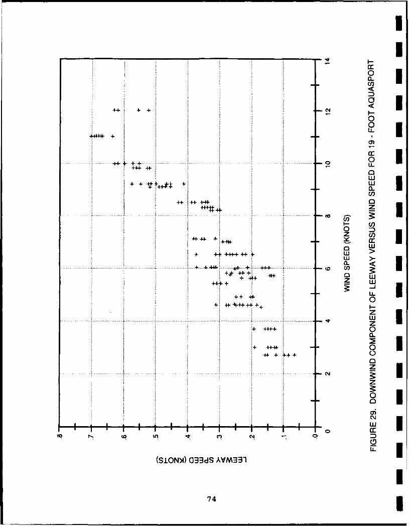
-4-4- +-.cJ0-0

4+ +. ..... 0

44-4-444#

+4- ~i~-4-444-

0

+ 4++4-

w

......- +44 .~4- +.....4 .... .. -44 ...... .. .......... I+#4 4+

w

0-+ 4-444--4+

*......... ............ ....................... ...... ............. ............ ......

:+ 4-i-44-4+4-+-4-4-+

0

C\

(P tfl Ci) N~ D

(SI0NN) (G3dS AVM31

741

TABLE 16

RESULTS OF LEEWAY MODELS FITTED TO DOWNWIND COMPONENT OF LEEWAY(L) FOR 19-FOOT OUTBOARD

(Values for L are in knots. W is wind speed in knots.)

Model Standard Error of: % VarianceSlope Estimate Explained

L - 0.0493W 0.00080 0.07003 81

L = -0.0851 + 0.0602W 0.00225 0.06448 84

4.6.3 20-Foot Cabin Cruiser

I Leeway data for the 20-foot cabin cruiser consist of 146 data

points collected over two days. An additional 45 data points

were collected; however, there was no suitable wind direction

information.

The 20-foot cabin cruiser drifted primarily stern to the wind

with RWDs lying between 120°R and 220°R. There is a weak

correlation between leeway angle and RWD caused by the craft not

responding to quick changes in wind direction. The leeway angles

ranged between 26 ° to the left and 270 to the right of downwind

(Figure 30). On average the 20-foot cabin cruiser appears to

drift downwind with little or no leeway angle.

Leeway speed appears to be a linear function of wind speed

(Figure 31). Both leeway models provide equivalent fits to the

3 downwind component of leeway (Table 17). The correlation between

the downwind component of leeway rate and wind speed is

negligible, as would be expected from the fit of the model

L - b*W to the leeway speed. Again, the model L = b*W is

recommended for simplicity, as the goodness-of-fits are similar.

75

cl

++ .+

+ LL

+ 0 ILii+4

+ +-+ + 4. U

+f ot++

+4+c++ 4

:++ . .a. 30+ +0U

+ 4+ I+ ++ + + 0

+ p- z

+ +

+ 4j++

+ 4+-4j

+ C;

w

0Ct,

(S33030 I'0VAM3760

I

TABLE 17 1RESULTS OF LEEWAY MODELS FITTED TO DOWNWIND COMPONENT OF LEEWAY

(L) FOR 20-FOOT CABIN CRUISER(Values for L are in knots. W is wind speed in knots.')

IModel Standard Error of: % Variance

Slope Estimate Explained

L - 0.0582W 0.00070 0.06066 84

L = -0.0813 + 0.0690W 0.00228 0.05631 86

IIIUIIIIIIII

CHAPTER 5

CONCLUSIONS

5.1 SUMMARY

The first step of this analysis was to identify the

equilibrium RWD for a craft due to its size and shape. The

second step was to determine the leeway angle and to compute the

component of leeway in the true leeway direction. The third step

was to fit a set of leeway models to that component of leeway.

Leeway equations for the craft tested are summarized in

Table 18. Canopied rafts with deep-draft ballast systems and

drogue (Switlik 4-man and Givens 6-man Rafts) are not included in

Table 18. These two rafts when drogued were found to have zero

or near zero leeway for winds up to 13 knots. These rafts with

drogues may have some as yet undetermined leeway speed for winds

greater than 13 knots.

5.2 IMPLICATIONS FOR CASP

Current leeway information available in CASP for the craft

tested is presented in this section. The CASP system uses leeway

rate, rate uncertainty, and leeway angle for search planning

(Section 1.2.1). Leeway rate is the ratio of leeway speed to

wind speed. For the craft tested in this experiment, (except the

Avon 4-man Raft) leeway rate is given in Table 18 as the

coefficient of W. Results of this experiment are used to

evaluate the leeway rates in CASP and to recommend changes.

There are seven classes of targets for leeway in the current

search planning doctrine. The leeway rates (Table 3) range from

a person in the water with zero leeway up to a light displacement

vessel without drogue which drifts at approximately 7% of the

windspeed. There are rules for adjusting leeway for the addition

of a canopy and ballast buckets on life rafts.

79

I

TABLE 18 3SUMMARY OF LEEWAY EQUATIONS AND ANGLES BY CRAFT I

(L - leeway speed; W = wind speed in knots. Positive leeway

angles denote deflection to the right of downwind.)

Class Craft Equation Leeway IAngle(s)

(degrees) II

Canopied Raft Switlik 4-Man Raft L = 0.0144W 0

with deep-draft without drogue

ballast system

Givens 6-Man Raft L = 0.0099W 0 Iwithout drogue 1

Canopied Raft Avon 4-Man Raft L =-0.1412+0.0213W* 0

with ballast without drogue

buckets *questionable equation

Canopied Raft Winslow 4-Man Raft L - 0.0490W 0 Iwith no ballast without drogue,

system full load,

combined swell ILight 14-Foot outboard L = 0.0398W +14, -24

displacement

vessels 19-Foot outboard L - 0.0493W 0

20-Foot Cabin L = 0.0582W 0 1Cruiser

80 3

Craft representing light displacement vessels with and

without drogues were tested in this experiment. In addition, an

entirely new class of craft was tested. The new class was

canopied rafts with deep-draft ballast system and drogue.

5.2.1 Canopied Rafts with DeeD-Draft Ballast System and Drogue

CASP does not currently include this type of craft in its

classification system. Leeway rates for the two rafts tested

from this classification (Switlik 4-man and Givens 6-man rafts)

were negligible at wind speeds below 13 knots. Leeway at wind

speeds in excess of 13 knots is unknown. The maximum deflection

from downwind for these rafts with drogue is not expected to

exceed 10° .

5.2.2 Canopied Rafts with DeeD-Draft Ballast System (No Drogue)

Current leeway doctrine classifies the undrogued Switlik

4-man and Givens 6-man rafts (canopied rafts with deep-draft

ballast systems) as light displacement vessels with drogue. CASP

uses a leeway rate of 0.05 and an uncertainty of 0.33 for these

vessels. This is equivalent to using a range of leeway rates

from 0.0335 to 0.0665. Leeway rates for the undrogued Switlik

4-man and Givens 6-man rafts did not fall into that range (Table

18). This confirms the results from the Summer 1983 Experiment

that these rafts drift more slowly than previously believed (Nash

and Willcox, 1985).

The leeway rate for the Switlik 4-man raft was 0.0144 and

the rate for the Givens 6-man raft was 0.0099 in this experiment.

The average of the two is 0.0122 with a rate uncertainty of 0.25,

well below values used in CASP. The rafts were found to have a

deflection off the downwind direction of 0° ± 100.

81

I

5.2.3 Canopied Rafts with Ballast Buckets mThe raft with canopy and ballast bags tested in this

experiment was the Avon 4-man raft. Current leeway doctrine has

this raft drifting at the same rate as an unballasted raft

without canopy, i.e., 7% of the wind. CASP uses a range of

leeway rates from 0.0469 to 0.0931 when the uncertainty is 3applied to the base leeway rate.

The leeway equation for the Avon 4-man raft gives leeway Ispeeds well below speeds calculated using the 0.07 base leeway

rate used by CASP. (Leeway speeds for CASP and the leeway 3equation for the Avon 4-man raft are compared in Table 11,

Section 4.4.1). In the Summer 1983 experiment, however, the

leeway of a raft with different ballast bags and canopy style was

found to be within present doctrine.

The authors recommend expanding the range of leeway rates to

cover both data sets. The recommended base rate is 0.05 with arate uncertainty of 0.96. No change is recommended for the

leeway angles.

5.2.4 Canopied Rafts without Ballast or Drogue 3The Winslow 4-man raft tested in this experiment was an

oblong canopied raft without any ballast system. Leeway rates

used by CASP range from 0.056 to 0.112. (The base rate of 0.07

is increased by 20% to compensate for the addition of a canopy.The range is calculated by applying the uncertainty of ±0.33 to

the new base rate of 0.084).

Leeway rates for the fully loaded Winslow 4-man raft are

slightly below the range used by CASP. Increasing the

uncertainty from 0.33 to 0.40 and using a base rate of 0.08 for a 3canopied raft without ballast or drogue will provide a range of

I82m

leeway rates that will include the rates observed for the

undrogued Winslow 4-man raft in this experiment. (The value 0.08

is based on a leeway of 0.0667 plus 20% for the addition of a

canopy). Leeway angles were within the recommended limits.

5.2.5 Light-Displacement Small Craft and Outboards

The three small boats tested (14-foot outboard, 19-foot

outboard and 20-foot cabin cruiser) fit into the classification

of light displacement vessels. The leeway rates used by CASP for

this classification are 0.0469 through 0.0931. Of the three

small craft, only the 14-foot outboard fell outside that range

(Table 18).

The 19-foot outboard and the 20-foot cabin cruiser drifted

downwind with their sterns to the wind. The 14-foot outboard

drifted beam to the wind and off the downwind direction by +14°

to -240, +100. This deflection off downwind is well within the

present doctrine for leeway angle, i.e., 350 on either side of

downwind.

Because one of the three small craft used in this experiment

had leeway rates lower than the present doctrine, the authors

recommend expansion of the rate limits. The proposed base rate

is 0.062 with a rate uncertainty of 0.50. No change in leeway

angles is recommended.

83

IIII

UI

(THIS PAGE INTENTIONALLY LEFT BLANK]I

IIIIIIIIII

84

APPENDIX A

DATA PROCESSING METHODS

A.1 INTRODUCTION

This appendix discusses methods used to process the raw data

to obtain leeway. The steps for reducing the data to a useful

form are:

1. Edit porition records and screen for bad positions.

2. Create interpolated position records using 2-minute

intervals.

3. Calculate the current at the test craft.

4. Calculate the test craft's velocities.

5. Calculate the leeway velocities of a test craft by

subtracting the current from the test craft's

velocities.

6. Screen the wind records for bad data and create 4-minute

vector averages of the wind.

7. Collate the leeway data, craft configurations, and wind

data into files suitable for analysis.

8. Calculate the leeway angle.

The processing of the position data through the calculation

of leeway is discussed in Section A.2 and its subsections. The

processing of the wind data is discussed in Section A.3 and its

subsections. The details of the collation of the leeway and wind

data with the associated parameters are discussed in Section A.4.

Leeway angle computations are discussed in Section A.5, and

leeway components are addressed in Section A.6.

A-1

I

A.2 POSITION DATA IFor this discussion, a platform may be either a drifter or a 3

test craft. A position refers to a data point consisting of a

time (T) and a corresponding location given in state plane m

coordinates. The x-coordinate (X) of a position is similar to

longitude, and the y-coordinate (Y) is similar to latitude. A

position record refers to a series of positions for a particular

platform corresponding to a continuous drift. For example, if a

drifter is deployed at 0900 and recovered at 1700 the same day, m

all positions and their corresponding times, from 0900 to 1700,

would represent a single position record. 3Position records were edited to contain only the time 3

interval during which the platform was freely drifting, and only

those positions provided by a single reference station of the

MTS. For reasons explained in Section 2.1.1, a position Idetermined using one reference station would differ from the

position determined using the other reference station. m

Next, a piecewisc linear xegression method was used to

screen position records for bad positions. This method is

described in Section A.2.1. Raw positions were compared to their

corresponding positions calculated from the regression equations.

If the difference between the raw and the calculated positions

was greater than 32.8 yards, the raw position was flagged as a [possible bad position. These candidates were checked and removed

if erroneous. m

Finally, the results of the linear regression were used to m

create interpolated-in-time position records for all platforms.

The interpolation served three purposes. The first was to make m

the position records suitable for velocity calculations by

ensuring that the time increment between a platform's successive

positions was constant (i.e., 120 seconds). The second purpose

was to produce position records for all platforms calculated at

A-2 m

exactly the same times, e.g., 12:00:00, 12:02:00, 12:04:00, etc.

The third purpose was to fill in data gaps of 6 minutes or less

caused by missing or deleted positions. Details of the

interpolation are discussed in Section A.2.1.

A.2.1 Piecewise Linear Regression Method

Position data were screened and interpolated using a

piecewise linear least-squares regression method. The term"piecewise" means that the regression used segments or pieces of

the data instead of using the entire data or position record.

For each segment of a position record, a linear regression

equation of each component of position (X,Y) as a function of

time (T) is fitted to the data using the method of least squares.

The method of least squares is a regression method that seeks to

ensure the best fit of the regression equation to the data by

minimizing the squares of the differences between the regression

line and the data. A full discussion of the method can be found

in most basic statistics books (e.g., Leplin, 1975). The

regression equations used are:

X - i+J*T Equation A-1

Y - k+l*T Equation A-2

where:

X is the east-west component of pcsition,

Y is the north-south component of position, and

i, J, k, and 1 are the coefficients determined by

the method of least squares.

For the screening, each position within the segment was

compared to its interpolated counterpart. The position would be

flagged as a possible bad position if the distance between the

raw position and its corresponding interpolated position was

greater than a critical value. After all possible bad positions

were flagged, another segment would be used so that each data

point was screened in at least two segments. Any data point

A-3

I

flagged twice %uld be checked prior to deletion. IThe screening program had five adjustable parameters.

Tyri --al values foz these parameters for the final screening are

presented in Table A-i. The regression was generally performed

on drift segments of 20 minutes. Segments of 10 minutes were

used when it appeared that the current was changing rapidly. The

minimum for the number of points required and maximum permissible

gap ensured that there were always adequate data for a

regression. If the segment contained fewer than the minimum m

number of points or contained a gap in the record greater than

the maximum permissible gap, another segment would be chosen. A 3time increment of 10 minutes would mean that a segment would

start 10 minutes after the start time of the previous segment.

Thus, if the first segment started at 1015, the next segment

TABLE A-I

PARAMETERS AND VALUES USED TO SCREEN AND INTERPOLATE

POSITION RECORDS

SCREENING VALUES

Segment Length: 1200 seconds (20 minutes) 3Minimum Number of Points: 5

Maximum Permissible Gap: 360 seconds (6 minutes)

Time Increment: 600 seconds (10 minutes)

Maximum Distance for Flag: 32.8 yards

INTERPOLATION VALUES IRegression Interval: 1200 seconds (20 minutes)

Minimum Number of Points: 7

Maximum Permissible Gap: 360 seconds (6 minutes)

Increment Interval: 120 seconds (2 minutes)

Maximum Distance for Flag: 32.8 yards

A-4 m

would start at 1025. The time increment was usually chosen to behalf of the segment length to screen each data point twice.

The interpolated records were created after the screeningfor questionable values. Each interpolated point was calculated

as the center point of a 20-minute segment with a 2-minuteincremental step. If the segment had less than seven points or a

gap greater than six minutes, the preceding interpolated point

was marked as the end of a drift and a new drift record started.

For the rest of the analysis, the two drift records were treated

as if they were of two different drifters.

A.2.2. Current Calculations

The current at each drifter was calculated for 4-minuteintervals from the interpolated drifter position records.

Because the interpolated drifter positions were spaced two

minutes apart, each 4-minute interval contained three positions.

The data from each drifter that was not drifting continuously

during the interval were discarded. The U and V components of

velocity for each remaining drifter were then calculated using a

time-centered finite difference algorithm. This means that U and

V were calculated as the difference between the first (T - t-2)

and last (T - t+2) positions for that time interval, ie.,

U(t) M X(t+2)- X(t-2) Equation A-3

4 minutes

V -y Eqaio -(t) " y(t+2)- (t-2) Equation A-4

4 minutes

where: t is the time of the center position,

t-2 is the time of the first position, and

t+2 is the time of the last position.

A-5

I

Then U(t ) and V(t ) were assigned to be the velocity components of Ithe drifter at the central time (t) of the interval. The output

for each active drifter consists of U(t) , V(t) , X(t) , and Y(t)"

A.2.3 Current Field Calculations

Current velocities at each drifter were combined to produce

a current field around the test craft. It was assumed that, for

each 4-minute interval, the rate of change of the current

velocity over the area covered by the drifters is constant. IMathematically stated, the assumptions for each 4-minute interval

are:

dU/dX - a Equation A-5

dU/dY - Equation A-6

dV/dX - 6 Equation A-7

dV/dY - r Equation A-8

where: U is the east/west component of current, 3V is the north/south component of current,

X is the east/west component of position, 3Y is the north/south component of position, and

a, 0, 6 and x are constants. 3The following regression equations were fitted to the

drifter velocity and position components (U(t), V(t), X(t), and

Y(t)) by the method of least squares:

U(t) * *X(t)+, Yt)+X Equation A-9

V(t) (t) Equation A-10where a, A, 8 and x are the constants defined above, and X and y

are constants determined by the regression for time (t).

These regression equations, when fitted to the data centered Ion a time interval, were taken to represent the current field for

A-6

that interval. The current at each test craft was calculated

using the center position of the test craft in the regression

equations.

The adequacy of the regression fit to the data was checked

by comparing the regression derived velocity for each drifter to

the observed velocities. If this difference for any component of

velocity for any active drifter was greater than 0.058 knots, the

regression in question was repeated for each test craft,

excluding the data for the drifter farthest from that test craft.

This procedure was repeated for each test craft until all

differences were 0.058 knots or less. The regression equations

will give a perfect fit to the data if there are three drifters.

Data were discarded for any interval with less than three

drifters continuously drifting.

A.2.4 Velocity Calculations

Test craft position data for 4-minute intervals were

generated from the interpolated position records produced by the

piecewise linear regression method described in Section A.2.1.

Test craft velocity components were calculated in the same manner

as the drifter velocity components. The position data were used

as inputs to the time-centered finite difference algorithm

(Equations A-3 and A-4) described in Section A.2.2. The

information generated for each test craft was U(t), V(t), X(t),

and Y(t) for each 4-minute interval.

A.2.5 Leeway Calculations

Leeway for each test craft was calculated for each 4-minute

interval by subtracting the current at the test craft from the

velocity of the test craft. The calculation yields leeway speed

and leeway direction.

A-7

m

A.3 WIND DATA

Wind data were collected from several sources during the

experiment, but only the data collected onboard the test craft

were used in the leeway calculations. Data from other sources

were used for quality control. All the test craft, except the

19-foot outboard, were equipped with automated instrument

packages. Onboard the 19-foot outboard, a student manually

recorded 1-minute averages of the wind every 20 minutes using the

Hercules 190 wind system. Data collected by the automated m

instrument packages were recorded every 20 to 40 seconds,

depending on the package's memory capacity.

A.3.1 Automated Instrument Package Data

Data from the automated instrument packages consist of

individual records of time and three analog voltages from the

compass, wind vane, and anemometer. Analog readings were

converted into engineering units. The wind direction was 3computed in degrees true. All craft used the same convention for

the bow of the craft and the orientation of the instrument

package. The instrument packages were installed with different

orientations based on expected wind direction to avoid the 50

dead zone of the wind vane potentiometer between 355 ° and 360 °

relative.

Wind data were visually checked and edited. Data from the

research vessels and the environmental buoy were used to quality

control data from the test craft. Suspect data values were

replaced by a missing value "flag" except when the problem could

be identified as one of two special cases. The first case

occurred when the compass heading or the relative wind direction

crossed the area of discontinuity between 355 ° and 360 ° . A

directional change from 359* to 0000 for the wind or the boat is

a 1 shift; however, for numbers and analog voltages, the

A-8

apparent shift is much greater. Even an averaging period of less

than three seconds was long enough for the wind vane sensor to

enter or cross the discontinuity area during a reading. Since

the average of a high number and a low number is a number in

between, the reading from the sensor can be in error up to 1800 .

Whenever this was identified to be the case, the bad value was

replaced by a default value corresponding to the middle of the

discontinuity. The maximum error associated with the substituted

value should be no more than 50. The second case was caused by a

manufacturing defect in one of the wind vanes. The vane's

housing and the potentiometer could became misaligned during

handling, resulting in a 190 offset. However, the data were

recoverable since the change in alignment could only occur when

the sensor was being mounted. The alignment of the installation

was checked before each run by taking several readings with the

vane aligned with the test craft.

The last step in processing the wind data was to create

4-minute vector averages which corresponded in time to the

drifter data record. These values were computed using compass

heading, relative wind direction, and wind speed. When the

compass heading or the- relative wind direction was missing, only

average wind speed was determined.

A.3.2 Brooks and Gatehouse Hercules 190 Data

Data from the Hercules 190 wind station consisted of 1-

minute averages of compass heading, wind direction, and wind

speed. These data were recorded every 20 minutes. The data were

compared with wind information from the other sources and found

to require no editing. Relative wind direction was computed.

Wind direction was converted to degrees true. A wind record with

values for every minute was created by assigning the nearest

values in time to each minute.

A-9

m

A.4 DATA COLLATION IAfter processing, the data consisted of 4-minute averages of

leeway speed and direction and the wind records. The wind

records included wind direction, wind speed, relative wind

direction, and compass heading. Data for each craft were

collated a day at a time. Records were combined only if their

times matched exactly. The combined records consisted of leeway

speed and direction, wind records, number of drifters used in

current calculations, and craft configuration parameters. (A m

craft's configuration consists of variables that may affect theleeway of the craft, such as the combined weight of the water

jugs onboard, deployment of a drogue, engine in the up or down

position, rudder position, etc.). Also included in the file arerecord-keeping items, such as the code for the craft and the date

and time of the individual data points.

A.5 LEEWAY ANGLE

The last computation was the leeway angle. For this report,

leeway angle is defined as the leeway direction minus the wind

direction with the convention of positive leeway angles for the

deflection to the right of downwind and negative to the left of

downwind.

A.6 LEEWAY COMPONENTS ILeeway speed was resolved into components. In most cases, m

the components used were the downwind and crosswind components of

leeway speed.

The only test craft with % non-zero leeway angle was the 14-

foot outboard. For the analysis of data for the 14-foot outboard

leeway speed was resolved into two components. One component was

mA-1O 1

in the leeway direction and the other component was perpendicular

to the leeway direction rather than in the downwind and crosswind

directions. The primary component of leeway was taken to be the

component of the leeway speed in the leeway direction (wind

direction plus leeway angle). The secondary component is

perpendicular to the primary component and positive in direction

to the right of the primary component.

A-11

IIIIII

[THIS PAGE INTENTIONALLY LEFT BLANK]i

IIIIIIIIIII

A-12 3

APPENDIX B

LEEWAY MODELS AND ERROR ANALYSIS

B.1 INTRODUCTION

The purpose of this appendix is to explain the various

relationships which are possible between leeway speed and wind

speed for different types of test craft and to determine the

angle of the drift with respect to the downwind direction.

Previous studies have assumed a linear relationship between

leeway speed and wind speed. This can be expressed

mathematically as:

L = b*W Equation B-i

where: L is the leeway speed,

W is the wind speed, and

b is the slope of the line (or leeway rate).

This is an equation for a straight line passing through the

origin. In terms of leeway, it means that when the wind speed is

zero, leeway speed will be zero.

A second linear equation that has been used to express the

relationship between leeway speed and wind speed is:

L = a+b*W Equation B-2

where: L is the leeway speed,

W is the wind speed,

a is the y-intercept, and

b is the slope of the line.

This is an equation for a straight line that may cross the y-axis

(or leeway axis) at some point other than zero. Equation B-2

B-1

I

allows for leeway cases where leeway speed is negligible below a ithreshold wind speed and increases with increasing wind speed

above the threshold wind speed.

When the value of a (the y-intercept) is close to zero,

Equations B-I and B-2 will produce similar results.

To investigate the possibility that the relationship between ileeway speed and wind speed is not linear, a third equation,

known as a power curve, was used in this analysis. The Irelationship is:

L = d*Wc Equation B-3

where: L is the leeway speed,

W is the wind speed, and

d and c are constants.

Equation B-3 removes the requirement implicit in the previous two

equations that the data (leeway as a function of wind speed) lie 3along a straight line. When the value of c is close to one,

Equations B-I and B-3 will produce similar results. The non

linear case in Equation B-3 was examined, but the results were

not significantly better than the linear results.

Methods used to determine a, and b are discussed in Section

B.2, and an error analysis is presented in Section B.3.

B.2 FITTING OF LEEWAY MODELS

The linear leeway models used for this analysis are repeated

below for convenience:

L - b*W Equation B-1

L - a+b*W Equation B-2

iI

8-2i

where: L is the leeway speed (or a component),

W is the wind speed, and

a and b are regression coefficients.

The models were fitted to the data using the least-squares

method. This means that all coefficients were chosen to minimize

the sum of the squares of the differences between the observed

and predicted leeway values. Equations B-1 and B-2 were solved

completely using the least-squares method.

The models all used the same definitions of degrees of

freedom (d.f.), standard error of estimate (Se), and coefficientof determination (r 2). The term degrees of freedom (d.f.) is

defined as the number of data points minus the number of

coefficients in the regression equation. The mathematical

definitions of Se and r2 are presented below:

Se (Y- ) /2 Equation B-4

A(y A 2 Equation B-5r2= 1Y (y - )

where: Y is an observed value of the dependent variable,AY is a predicted value of the dependent variable,

Y is the mean of the dependent variable,

is the summation sign, and

n is the number of points used in fitting the line.

The dependent variable is the variable which is predicted,

i.e., leeway. The standard error of estimate (Se) is a measure

of the variability of the dependent variable around theregression line with 68% and 95.5% of the observations lying

within one or two (Se) of the regression line. The coefficient

of determination (r 2 ) is the ratio of the variability in the

dependent variable explained by the regression equation to the

B-3

I

original variability around the mean observations. A value for Ir2 of 1.0 would be a perfect fit of the data. The value of r2

lies between 0.0 and 1.0. Generally, regressions with r2 values

of less than 0.1 are useless, of 0.2 to 0.4 are poor, of 0.5 or

greater are good, and of greater than 0.8 are excellent.

Next, the fitting of the leeway models is described

separately. The descriptions will use the standard notations ofX and Y instead of W and L to avoid confusion. W can be

substituted for X and L for Y. I

L - b*W or Y - b*X 3A good reference for this regression equation is Snedecor

and Cochran (1980). The coefficient (b) for the method of least-squares is defined as that value of b which minimizes the sum of

the squares of differences between the observed and predictedvalues of the dependent variable (Y). Mathematically stated:

(Y - Y) = 0 Equation B-6

and (y _ y)2 is a minimum m

where: Y is an observed value of the dependent variable,

AIY is a predicted value of the dependent variable,

and

b is the regression coefficient.

The standard error of the slope (Sa) is calculated by the

following equation (Snedecor and Cochran, 1980, page 155):

Sa = Se/NjX 2 Equation B-7 Iwhere: (Se) is the standard error of estimate.

II

5-4 i

The standard 6rror of the slope is a measure of the variability

of the slope of the regression. It is used to calculate the

confidence limits on the slope.

L - a+b*W or Y - a+b*X

The standard regression equations for this model are

(Laplin, 1975):

b XY - NXY Equation B-8b = - NX2

a = 1 - bR Equation B-9

Sa = Se Equation B-10

(FX 2 - NX2)l/2

where: a is the regression coefficient of the intercept,

b is the regression coefficient of the slope,

N is the number of data points,

X is the independent variable (wind speed),

Y is the dependent variable (leeway speed),

is the summation sign,

, are the average or mean values of X and Y,

Se is the standard error of estimate, and

Sa is the standard error of the slope (b).

The standard error of the slope is a measure of thevariability of the slope of the regression. It is used tocalculate the confidence limits on the slope.

B.3 ERROR ANALYSIS

Section 2.1.1 and Appendix A discussed the sources of error

B-5

I

involving the tracking system and wind instruments. Both were m

calibrated just before the experiment and checked during and

after the experiment. The remaining errors arose from normal

measurement errors and assumptions made during data reduction and

analysis. This analysis will attempt to estimate the magnitude

of the errors associated with the leeway and wind velocities.

Errors associated with leeway velocities are determined by Iestimating the error in the current value at the test craft.

Data for 8 April 1985 were chosen to check the current

calculations because of the long drift records and the large

number of drifters. Each drifter was treated as a test craft,

and the current was estimated from the remaining drifter array.

The current was separated into north-south and east-west

components. The absolute differences between predicted and

observed components of current were recorded for 222 predictions.

The predicted current explained about 55% of the variability in

the observed current for both components. The maximum magnitudes

of the observed east-west and north-south components of current 3were 0.23 knots and 0.76 knots respectively. The maximum errors

were ±0.087 knots and ±0.105 knots. The magnitude of the errors 3had no correlation with the magnitude of either component of the

predicted or observed current, magnitude of the other error

component, or the number of drifters used to make the prediction.

The root mean square (rms) of the errors was ±0.031 knots for the

east-west component and ±0.037 knots for the north-south

component. To estimate the propagation of the errors through the

leeway calculation, it is assumed that the addition of two errors

(E1 and E2 ) is as follows: ISum of Errors - 2+E 2 Equation B-11

III

B-6m

This leads to an estimate of the error in the current

calculations of +0.049 knots. A very conservative estimate of

the error in the test craft velocity is that it is the same as

the error in the current calculations. Using Equation B-11, the

error associated with the leeway velocities is ±0.068 knots.

The accuracy of the wind measurements is given in Section

2.1.2 for the automated instrument packages as better than +10°

and ±0.97 knots. The component of leeway used to calculate the

relationship of leeway to wind speed is computed on the basis of

the wind direction. A 100 error in wind direction would lead to

the leeway being underestimated by 2%. Assuming that a craft

drifts at 7% of the wind and the wind speed is 19.4 knots, the

total error in the leeway from the angular and speed errors would

be +0.097 knots.

Two approximations were made in the data reduction and

analysis that may not be obvious. First, the wind is assumed to

be the apparent wind relative to the current, i.e., the wind as

measured by an object drifting with the current. Using this

apparent wind eliminates the need to consider such cases as wind

with and wind opposing the current. The fact that the wind

instrument is on a craft with leeway is ignored as the leeway

speed is assumed to be 10% or less of the wind speed.

The second assumption is that a steady-state situation

exists over each 4-minute time step. Reality is that the craft

was probably accelerating during these intervals and was never in

perfect balance with the wind. Both of these approximations are

thought to have little or no effect on the results.

B-7

IIIIIII

[THIS PAGE INTENTIONALLY LEFT BLANK]i

iiiIIiiiiI

B-8 3

APPENDIX C

OBSERVATIONS AND RECOMMENDATIONS

C.1 PROPOSED EXPERIMENTAL METHOD OF DETERMINING LEEWAY

During this experiment, leeway was determined indirectly

from other parameters. An electromagnetic current meter, which

determines the water current flowing through a magnetic field,

may provide a method of measuring leeway directly without a

tracking system and the large number of personnel currently

required. The electromagnetic current meter can accurately

measure very small velocities needed for leeway experiments.

Previous current meter designs suffered from wave pumping or

could not measure very small velocities.

The new method consists of equipping the test craft with

both a wind instrument, as is done currently, and a current meter

suspended under the craft. The current meter would measure the

motion of the craft through the water, i.e., leeway, directly.

The data would be contaminated by wave motion, which would have

to be filtered out. The filtering could be done by either

spectral analysis or vector averaging over a 10- to 15-minute

period.

The drag of the current meter would be negligible for craft

such a sailboats with keels, cabin cruisers, and larger vessels.

Conducting a test of the proposed method while using the current

method would permit any effect of the additional drag of the

current meter to be identified.

The proposed method would require development of an

instrument package onboard the test craft suitable to support a

current meter and wind instrument. If successful, the method

would permit the collection of leeway data without the constant

maintenance of a drifter array and tracking system. Leeway data

for high wind conditions could be collected by deploying a test

C-1

I

craft before the experiment begins and leaving it unattended.

Tracking could be done either by satellite (Murphy and Allen,

1985) or by a LORAN-C rece-ve-. and relay.

C.2 RESEARCH TOPICS

The following leeway topics need further research.

1. Variations in leeway caused by different degrees of loading

on a craft should be determined. The maximum and minimum

leeway values should be obtained by testing the craft fully

loaded and empty.

2. The leeway of a craft greater than 25 feet in length should

be checked. The authors know of no successful work done in

this area since 1960 (Chapline, 1960).

3. The rafts referred to as canopied rafts with ballast buckets 3need to be researched as a group. Regulations have required

the addition of more ballast to this type of raft than they

had in the early 1970's. Variations in ballast

configurations for this group could affect leeway.

4. Leeway data need to be collected for higher wind speeds to

gain a better understanding of leeway. This may require the 3development of new or modified methods of determining

leeway.

IIII

C-2I

REFERENCES

National Search and Rescue Manual, 1986. U. S. Coast Guard,

COMDTINST M16120.5 dtd 1 August 1986.

Allen, A.A., S. L. Eynon, and R. Q. Robe. 1987. "Descriptions of

HF and VHF Loran-C Buoys and Evaluations as Potential Datum

Marker Buoys." U.S. Coast Guard Report CG-D-02-88.

Central Tactics and Trial Organization (CTTO). 1974. "Life Raft

Drift Rates." CTTO/10756/44/LRMP, Canada.

Chapline, W.E. 1960. "Estimating the Drift of Distressed Small

Craft." Coast Guard Alumni Association Bulletin, U.S. Coast Guard

Academy, New London, CT. Vol. 22, No. 2, March-April 1960, p.

39-42.

Edwards, N.C., Jr., S.R. Osmer, T.J. Mazour, and G.L. Hover.

1981. "Factors Affecting Coast Guard SAR Unit Visual Detection

Performance." U.S. Coast Guard Report CG-D-09-82.

Hufford, G.L., and S. Broida. 1974. "Determination of Small

Craft Leeway." U.S. Coast Guard Research and Development Center

Report No. 39/74, December 1974.

Laplin, L. 1975. STATISTICS. Meaning and Method, Harcourt Brace

Jovanovich, Inc., New York, NY.

Nash, L., and J. Willcox. 1985. "Summer 1983 Leeway Drift

Experiment." U.S. Coast Guard Report CG-D-35-85.

Morgan, C.W. 1978. "Seven-Man Life Raft Leeway Study." U.S.

Coast Guard Oceanographic Unit Technical Report 78-1, Washington,

D.C.

R-1

I

REFERENCES (Cont'd)

Morgan, C.W., S.E. Brown, and R.C. Murrell. 1977. "Experiments Iin Small Craft Leeway." U.S. Coast Guard Oceanographic Unit

Technical Report 77-2, Washington, D.C.

Murphy, D.L., and Allen, A.A. 1985. "An Evaluation of CASP Drift

Predictions Near the New England Shelf/Slope Front." U.S. Coast

Guard Report CG-D-16-85.

Osmer, S.R., N.C. Edwards, Jr., and A.L. Breiter. 1982. "An

Evaluation of Life Raft Leeway, February 1982." U.S. Coast Guard IReport No. CG-D-10-82 IPingree, F. deW. 1944. "Forethoughts on Rubber Rafts." Woods

Hole Oceanographic Institution, 26pp.

Scobie, R.W., and D.L. Thompson. 1979. "Life Raft Study,

February 1978." U.S. Coast Guard Oceanographic Unit Technical

Report 79-1, Washington, D.C.

Snedecor, W., and W.G. Cochran. 1980. Statistical Methods,

Seventh Edition. Iowa State University Press, Ames, Iowa.

IUIIII

R-2 3